Chai, Hui and Ho, Wai and Graham, Neil and May, Sean and Massawe, Festo and Mayes, Sean (2017) A cross-species gene expression marker-based genetic map and QTL analysis in bambara groundnut. Genes, 8 (3). p. 84. ISSN 2073-4425

Access from the University of Nottingham repository: http://eprints.nottingham.ac.uk/40897/1/genes-08-00084-v2.pdf

Copyright and reuse:

The Nottingham ePrints service makes this work by researchers of the University of Nottingham available open access under the following conditions.

This article is made available under the Creative Commons Attribution licence and may be reused according to the conditions of the licence. For more details see: http://creativecommons.org/licenses/by/2.5/

A note on versions:

The version presented here may differ from the published version or from the version of record. If you wish to cite this item you are advised to consult the publisher’s version. Please see the repository url above for details on accessing the published version and note that access may require a subscription.

For more information, please contact eprints@nottingham.ac.uk

genesG C A T

T A C G

G C A T

Article

A Cross-Species Gene Expression Marker-BasedGenetic Map and QTL Analysis inBambara Groundnut

Hui Hui Chai 1,*, Wai Kuan Ho 1,2, Neil Graham 3, Sean May 3, Festo Massawe 1,2

and Sean Mayes 1,2,3

1 Biotechnology Research Centre, School of Biosciences, University of Nottingham Malaysia Campus,Jalan Broga, Semenyih 43500, Selangor Darul Ehsan, Malaysia; waikuan@cffresearch.org (W.K.H.);Festo.Massawe@nottingham.edu.my (F.M.); sean.mayes@cffresearch.org (S.M.)

2 Crops For the Future, Jalan Broga, Semenyih 43500, Selangor Darul Ehsan, Malaysia3 Plant and Crop Sciences, School of Biosciences, University of Nottingham, Sutton Bonington Campus, Leics,

Loughborough LE12 5RD, UK; neil.graham@nottingham.ac.uk (N.G.); sean.may@nottingham.ac.uk (S.M.)* Correspondence: Huihui.Chai@nottingham.edu.my; Tel.: +60-(03)-8725 3616

Academic Editor: J. Peter W. YoungReceived: 5 December 2016; Accepted: 11 January 2017; Published: 22 February 2017

Abstract: Bambara groundnut (Vigna subterranea (L.) Verdc.) is an underutilised legume crop, whichhas long been recognised as a protein-rich and drought-tolerant crop, used extensively in Sub-SaharanAfrica. The aim of the study was to identify quantitative trait loci (QTL) involved in agronomic anddrought-related traits using an expression marker-based genetic map based on major crop resourcesdeveloped in soybean. The gene expression markers (GEMs) were generated at the (unmasked)probe-pair level after cross-hybridisation of bambara groundnut leaf RNA to the Affymetrix SoybeanGenome GeneChip. A total of 753 markers grouped at an LOD (Logarithm of odds) of three, with527 markers mapped into linkage groups. From this initial map, a spaced expression marker-basedgenetic map consisting of 13 linkage groups containing 218 GEMs, spanning 982.7 cM (centimorgan)of the bambara groundnut genome, was developed. Of the QTL detected, 46% were detected inboth control and drought treatment populations, suggesting that they are the result of intrinsic traitdifferences between the parental lines used to construct the cross, with 31% detected in only one ofthe conditions. The present GEM map in bambara groundnut provides one technically feasible routefor the translation of information and resources from major and model plant species to underutilisedand resource-poor crops.

Keywords: Affymetrix GeneChip; cross-hybridisation; gene expression markers; quantitativetrait loci

1. Introduction

Bambara groundnut (Vigna subterranea (L.) Verdc) is an indigenous legume crop grown mainlyby subsistence and small-scale farmers in Sub-Saharan Africa. This legume species is the third mostimportant legume after groundnut (Arachis hypogaea) and cowpea (Vigna unguiculata) in semi-aridAfrica [1]. In addition to relatively high protein content in bambara groundnut seed (18%–26%) [2,3],bambara groundnut is also recognised for its good drought tolerance and ability to grow in poor soils,the latter partly as a result of fixing nitrogen from the atmosphere.

Being a relatively neglected crop species, the cultivation of bambara groundnut has mainly reliedon local experience and indigenous knowledge [4]. There are few established varieties of bambaragroundnut, and most of the bambara groundnut accessions exist in the form of landraces [5]. Analysisusing co-dominant markers [6] revealed that bambara groundnut is highly inbred, with seed from a

Genes 2017, 8, 84; doi:10.3390/genes8020084 www.mdpi.com/journal/genes

Genes 2017, 8, 84 2 of 19

single plant essentially representing an inbred line, although relatively high levels of genetic variationwere observed between plants from the same landrace accession. Screening landraces could providebreeders with genetic resources to improve yield, biotic and abiotic resistance and the adaptability ofthe crop to various environments.

To understand the genetic architecture of bambara groundnut for breeding purposes, it is usefulto develop a high density genetic linkage map. A genetic map facilitates the identification of importantgene-containing regions prior to positional cloning or the use of flanking markers for marker-assistedselection (MAS) in breeding programmes. Genetic maps can assist with conserved synteny mapping,where markers can be located in the species of origin and comparisons made with the species wheregreater resources and trait knowledge exist. The first genetic map in bambara groundnut (2n = 2x = 22)was reported by Basu et al. [7] using an F2 segregating population derived from a controlled crossbetween an ancestral wild-type (VSSP11) and the domesticated form (a genotype derived from theDipC landrace) of bambara groundnut on the basis of differences observed in growth habit, maturityand yield performance. Twenty linkage groups were identified using 67 AFLP (Amplified FragmentLength Polymorphism) markers and one SSR (Simple Sequence Repeat) marker, giving a total length of516 cM (centimorgan), with the inter-marker distance varying from 4.7 cM to 32 cM [7]. A quantitativetrait loci (QTL) analysis localised four QTL controlling 100-seed weight, specific leaf area, numberof stem per plant and carbon (Delta C13) isotope discrimination through the use of this interspecificgenetic map [8]. In addition, Ahmad et al. (2016) [9] reported the construction of the first intraspecificgenetic map using an F3 segregating population derived from a cross between genotypes derivedfrom two domesticated landraces, Tiga Nicuru and DipC. The intraspecific map covered 608.3 cM over21 linkage groups and included 29 SSR and 209 microarray-based DArT markers, with marker-markerdistances ranging between 0 cM and 10.1 cM. QTL analysis allowed the mapping of 36 significant QTLfor 19 agronomic traits, including internode length, peduncle length and biomass dry weight [9].

Construction of genetic maps has employed various types of DNA-based markers, whilegene-based microarrays have been widely adopted in recent years to generate large-scale expressiondata. Recently, microarrays have been increasingly used to generate expression-based markerinformation, such as gene expression markers (GEMs), for the development of an expression-basedgenetic map, followed by comprehensive conventional quantitative trait locus (QTL) and expressionquantitative trait loci (eQTL) studies [10–14]. GEMs refer to significant differences in the hybridisationsignal strength between individuals when cRNA is hybridised to GeneChip arrays. The differences inhybridization strength observed between individuals could be due to either sequence polymorphismseffecting the hybridization efficiencies of nucleic acids to individual features on the microarrays oractual differences in the transcript (mRNA) abundance. In a structured population, such as a series ofrecombinant inbred lines (RILs) derived from a controlled cross, these differences can be interpreted asgenetic markers for map construction. In one Brassica eQTL experiment, the majority of GEMs wereselected based on differences in hybridisation signal intensity in the parental plants. These were likelyto have resulted from (but were not unequivocally proven to be) sequence polymorphisms, whicheffected the binding of the test RNA samples to the microarray targets [14]. Using a genetic mapconstructed from 125 GEMs, Hammond et al. (2011) [14] showed that the identification of regulatoryhotspots that regulated low phosphorus response in B. rapa was possible.

The potential for analysing less intensively studied species (such as bambara groundnut)using GEMs derived from a microarray was demonstrated when Hammond et al. (2005) [15]reported the hybridisation of RNA derived from Brassica oleracea L. plants responding to mineralnutrient (phosphorus; P) stress on the Affymetrix GeneChip designed for Arabidopsis, followed bythe identification of 99 genes that were significantly different between parental samples under Pstress in B. oleracea. The approach adopted, which uses microarrays developed for a given speciesto analyse another related species, is known as the XSpecies (cross-species) microarray approach(http://affy.arabidopsis.info/xspecies/). Affymetrix GeneChip microarrays can provide reproducibleand accurate data, which can be compared across experiments. While custom genotyping arrays for

Genes 2017, 8, 84 3 of 19

species with genome sequence information could be designed despite the high manufacturing costsfor a microarray, thirteen Affymetrix GeneChip microarrays are currently publicly available for limitednumbers of plant species [16]. The XSpecies microarray approach, which is one of the approachesdeveloped for the Affymetrix GeneChip platform, offers a potential approach to research crop specieswhere no species-specific microarray is publically available. In addition to Brassica, the XSpeciesmicroarray approach has been used in crop species, such as wheat (Triticum aestivum) [17], cowpea [18],banana (Musa) [19], sorghum (Sorghum bicolor) [20] and blueberry (Vaccinium corymbosum) [21].

The application of QTL analysis can lead to the identification of candidate genes that control theobserved traits. For instance, a QTL for beginning of flowering in pea was mapped onto linkage groupLGV at 49 cM [22], which harbours the gene, DET, that is involved in the regulation of flowering timeand inflorescence architecture [23]. Using extensive genomic resources developed in major crops orclosely-related species, conserved syntenic loci and potential candidate genes that control importantagronomic traits in bambara groundnut could be detected by projecting the map of QTL onto a physicalmap or genetic map based on functional markers derived from closely-related species, such as soybean(Glycine max) and common bean (Phaseolus vulgaris).

The aim of this study was to identify the locations of quantitative trait loci for a wide range ofagronomic traits displayed in a bambara groundnut F5 segregating population using the XSpeciesapproach, with microarray resources developed in soybean. Following cross-hybridisation of RNAfrom bambara groundnut to the Affymetrix Soybean Genome GeneChip, an expression-based geneticmap (GEM map) was constructed and utilised for a comprehensive QTL analysis. The present GEMmap will serve as a platform for conserved synteny mapping with closely-related crop species, suchas soybean and common bean, for possible transfer of positional information, creation of conservedsynthetic links and identification of candidate genes and gene regions for breeding.

2. Materials and Methods

2.1. Plant Material

An F5 segregating population was derived from a controlled cross between single genotypesderived from the Tiga Nicuru (maternal) and DipC (paternal) landraces. The irrigated populationreceived a continuous watering regime, while the drought treatment population was subjected toa 42-day cumulative mild drought treatment starting at 50 DAS (days after sowing) by withholdingirrigation prior to genetic linkage analysis. Plant material, consisting of parental lines and 65 F5

individual lines, was planted in a controlled environment glasshouse at the FutureCrop Glasshouses,Sutton Bonington Campus, the University of Nottingham, U.K. The details of the plant material andexperimental design were reported in Chai et al. (2016) [24].

2.2. RNA Preparation and Cross-Hybridisation

After bambara groundnut parental lines and the drought treatment F5 segregating populationhad received six weeks of drought treatment, two leaves from each of the individual plants wereharvested. In total, 77 biological samples were collected, comprising one biological replicate foreach line from the drought treatment plot (n = 65) and three replicates of each parental line underdrought and irrigation conditions (3 replicates × 2 parents × 2 treatments = 12). The leaf sampleswere then transferred to a −80 ◦C freezer for longer term storage. Total RNA was extracted using theQiagen RNeasy Plant Mini Kit (Qiagen, Manchester, U.K.) according to the manufacturer’s instructions.The final RNA was resuspended in 30 µL RNase-free water. Total RNA was checked for integrity andquality using both the Agilent 2100 Bioanalyzer (Agilent Technologies, Santa Clara, CA, USA) and gelelectrophoresis. A total of 10 µL of RNA samples (100 ng·µL−1) derived from the 12 parental samplesand 65 individual lines were sent to the NASC Affymetrix Service, UoN, Sutton Bonington Campus,U.K., for cross-hybridisation analysis onto the Affymetrix Soybean Genome GeneChip.

Genes 2017, 8, 84 4 of 19

2.3. Generation of GEMs

A total of 77 data files was generated and initial data analysis performed using GeneSpring GX(Version 11.0.2; Agilent Technologies). The analysis approach adopted for bambara groundnut datawas based on, but modified from, Hammond et al. (2011) [14], which used B. rapa as the experimentalorganism. Three sets of normalised data were produced at three different levels: probe-sets, chipdefinition file (CDF) masked probe-sets and unmasked probe-pairs (oligonucleotide). A new customCDF file was created using PIGEONSv1.2 software [25] by filtering the original Tiga Nicuru CDF fileand DipC CDF file at a signal threshold of 141. The custom CDF file was then used to mask the signalsderived from each probe-set in order to generate a custom masked probe-set dataset. The three sets ofnormalised chip data were used to generate potential GEMs. The mean and standard deviation (s.d.)of each log2-normalised hybridisation signal were calculated for each of the parents and segregatingpopulation, followed by provisionally assigning allele scores “a” and “b” to each individual line foreach putative marker, depending on if the hybridisation signal of individual line was on the same sideof the mean population signal as the maternal (Tiga Nicuru) or parental (DipC) values (SupplementalText S1). A good separation between group “a” and group “b” was indicated by high “distinctness”score. The probe-sets or probe-pairs in their respective normalised datasets with distinctness scoreequal or higher than a selected threshold value were selected as potential GEMs. The threshold valuesof markers used in map construction were retrospectively checked through visual inspection of thegraphical distribution of group “a” and group “b”. A good separation of “a” and “b” allele scoreswithin the individual lines would allow the production of polymorphic GEMs of good quality.

2.4. Development of Expression-Based Linkage Map Using GEMs

The GEM map was constructed using JoinMap v4.1 [26]. A combination of regression mapping(RM) and maximum likelihood mapping (MLM) approaches with grouping at LOD ≥ 3 was applied toobtain the GEM order for each linkage group. The Haldane mapping function was used with defaultsettings: recombination fraction ≤4.0, ripple value = 1, jump in goodness-of-fit threshold = 5. The orderof GEMs was tested by comparing the results from RM and MLM. Miscalled GEMs showing doublerecombination events in individual lines within genetic distances between 1 and 3 cM were removed.The reiterative process of marker removal on the basis of visual inspection of graphical genotypes andby examining “fit and stress” parameters enables a high quality spaced framework map consisting ofGEMs to be generated for further development and used as the basis for QTL analysis. Due to theinsufficient linkage to complete the map using RM for linkage groups LG6 and LG8, these groups weredivided into subgroups ”A” and “B”, respectively. However, MLM indicated that they were actuallypart of the same linkage groups.

2.5. Identifying Significant QTL

Data from a range of morphological and physiological traits, including days to emergence, daysto flowering, estimated days to podding, internode length, peduncle length, pod number per plant,pod weight per plant, seed number per plant, seed weight per plant, 100-seed weight, shoot dry weightand harvest index, and drought-related traits, including stomatal conductance, relative water content,stomatal density, leaf carbon (Delta C13) isotope analysis (CID) and leaf (Delta N15) isotope analysis(NID), were checked for normality and transformed, if necessary, as reported in Chai et al. (2016) [24]before being subjected to QTL analysis. MapQTL® v6.1 (Kyazma, Wageningen, Netherlands) with acombination of two mapping approaches, interval mapping (IM) and multiple QTL mapping (MQM),was used to identify the QTL. The analysis options were set as default, including using the regressionalgorithm for IM and MQM mapping and fitting dominance for the population types. The permutationtest using 10,000 reiterations was first conducted in order to determine the expected significancethreshold of the LOD score, followed by IM mapping. Significant QTL were identified if the LODscore obtained from IM mapping was equivalent or higher than the genome-wide (GW) threshold

Genes 2017, 8, 84 5 of 19

at p ≤ 0.05 as derived from the permutation test. QTL were considered as ‘putative’ when the LODscore was lower than the GW threshold by up to one LOD. Once QTL with significant LOD scoreswere identified from the IM mapping model, the closest linked marker was selected as a cofactorprior to MQM mapping. If the result from MQM mapping showed a significant LOD score somedistance away (a minimum of 20 cM) from the marker cofactor, automated cofactor selection (ACS)was applied for cofactor selection and MQM mapping repeated. The positions of QTL picked upby marker cofactors were verified through visual inspection of the LOD profile and the LOD tableproduced by MapQTL® v6.1.

3. Results

3.1. Novel Gene Expression Markers

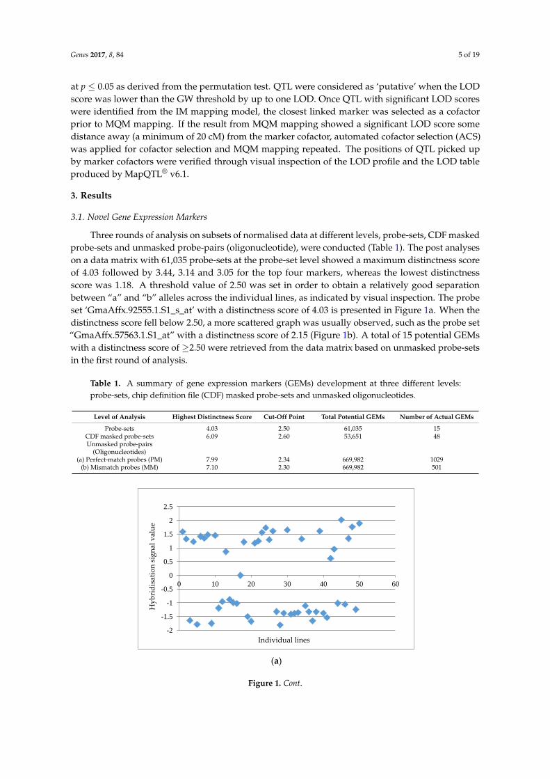
Three rounds of analysis on subsets of normalised data at different levels, probe-sets, CDF maskedprobe-sets and unmasked probe-pairs (oligonucleotide), were conducted (Table 1). The post analyseson a data matrix with 61,035 probe-sets at the probe-set level showed a maximum distinctness scoreof 4.03 followed by 3.44, 3.14 and 3.05 for the top four markers, whereas the lowest distinctnessscore was 1.18. A threshold value of 2.50 was set in order to obtain a relatively good separationbetween “a” and “b” alleles across the individual lines, as indicated by visual inspection. The probeset ‘GmaAffx.92555.1.S1_s_at’ with a distinctness score of 4.03 is presented in Figure 1a. When thedistinctness score fell below 2.50, a more scattered graph was usually observed, such as the probe set“GmaAffx.57563.1.S1_at” with a distinctness score of 2.15 (Figure 1b). A total of 15 potential GEMswith a distinctness score of ≥2.50 were retrieved from the data matrix based on unmasked probe-setsin the first round of analysis.

Table 1. A summary of gene expression markers (GEMs) development at three different levels:probe-sets, chip definition file (CDF) masked probe-sets and unmasked oligonucleotides.

Level of Analysis Highest Distinctness Score Cut-Off Point Total Potential GEMs Number of Actual GEMs

Probe-sets 4.03 2.50 61,035 15CDF masked probe-sets 6.09 2.60 53,651 48Unmasked probe-pairs

(Oligonucleotides)(a) Perfect-match probes (PM) 7.99 2.34 669,982 1029

(b) Mismatch probes (MM) 7.10 2.30 669,982 501

Genes 2017, 8, 2 5 of 18

as ‘putative’ when the LOD score was lower than the GW threshold by up to one LOD. Once QTL

with significant LOD scores were identified from the IM mapping model, the closest linked marker

was selected as a cofactor prior to MQM mapping. If the result from MQM mapping showed a

significant LOD score some distance away (a minimum of 20 cM) from the marker cofactor,

automated cofactor selection (ACS) was applied for cofactor selection and MQM mapping repeated.

The positions of QTL picked up by marker cofactors were verified through visual inspection of the

LOD profile and the LOD table produced by MapQTL® v6.1.

3. Results

3.1. Novel Gene Expression Markers

Three rounds of analysis on subsets of normalised data at different levels, probe-sets, CDF

masked probe-sets and unmasked probe-pairs (oligonucleotide), were conducted (Table 1). The post

analyses on a data matrix with 61,035 probe-sets at the probe-set level showed a maximum

distinctness score of 4.03 followed by 3.44, 3.14 and 3.05 for the top four markers, whereas the lowest

distinctness score was 1.18. A threshold value of 2.50 was set in order to obtain a relatively good

separation between “a” and “b” alleles across the individual lines, as indicated by visual inspection.

The probe set ‘GmaAffx.92555.1.S1_s_at’ with a distinctness score of 4.03 is presented in Figure 1a.

When the distinctness score fell below 2.50, a more scattered graph was usually observed, such as the

probe set “GmaAffx.57563.1.S1_at” with a distinctness score of 2.15 (Figure 1b). A total of 15 potential

GEMs with a distinctness score of ≥2.50 were retrieved from the data matrix based on unmasked

probe-sets in the first round of analysis.

Table 1. A summary of gene expression markers (GEMs) development at three different levels: probe-

sets, chip definition file (CDF) masked probe-sets and unmasked oligonucleotides.

Level of Analysis Highest

Distinctness Score

Cut-Off

Point

Total Potential

GEMs

Number of

Actual GEMs

Probe-sets 4.03 2.50 61,035 15

CDF masked probe-sets 6.09 2.60 53,651 48

Unmasked probe-pairs

(Oligonucleotides)

(a) Perfect-match probes (PM) 7.99 2.34 669,982 1029

(b) Mismatch probes (MM) 7.10 2.30 669,982 501

(a)

-2

-1.5

-1

-0.5

0

0.5

1

1.5

2

2.5

0 10 20 30 40 50 60

Hy

bri

dis

atio

n s

ign

al v

alu

e

Individual lines

Figure 1. Cont.

Genes 2017, 8, 84 6 of 19

Genes 2017, 8, 2 6 of 18

(b)

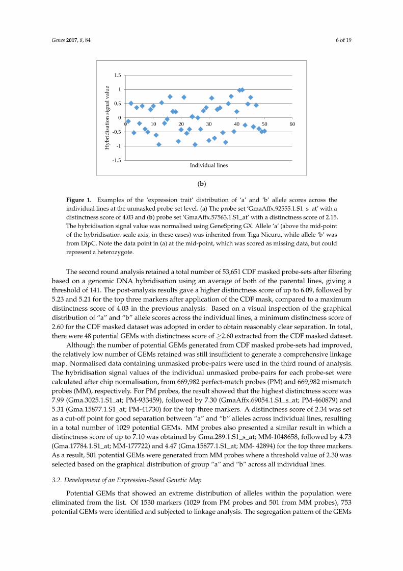
Figure 1. Examples of the ‘expression trait’ distribution of ‘a’ and ‘b’ allele scores across the individual

lines at the unmasked probe-set level. (a) The probe set ‘GmaAffx.92555.1.S1_s_at’ with a distinctness

score of 4.03 and (b) probe set ‘GmaAffx.57563.1.S1_at’ with a distinctness score of 2.15. The

hybridisation signal value was normalised using GeneSpring GX. Allele ‘a’ (above the mid-point of

the hybridisation scale axis, in these cases) was inherited from Tiga Nicuru, while allele ‘b’ was from

DipC. Note the data point in (a) at the mid-point, which was scored as missing data, but could

represent a heterozygote.

The second round analysis retained a total number of 53,651 CDF masked probe-sets after

filtering based on a genomic DNA hybridisation using an average of both of the parental lines, giving

a threshold of 141. The post-analysis results gave a higher distinctness score of up to 6.09, followed

by 5.23 and 5.21 for the top three markers after application of the CDF mask, compared to a maximum

distinctness score of 4.03 in the previous analysis. Based on a visual inspection of the graphical

distribution of “a” and “b” allele scores across the individual lines, a minimum distinctness score of

2.60 for the CDF masked dataset was adopted in order to obtain reasonably clear separation. In total,

there were 48 potential GEMs with distinctness score of ≥2.60 extracted from the CDF masked dataset.

Although the number of potential GEMs generated from CDF masked probe-sets had improved,

the relatively low number of GEMs retained was still insufficient to generate a comprehensive linkage

map. Normalised data containing unmasked probe-pairs were used in the third round of analysis.

The hybridisation signal values of the individual unmasked probe-pairs for each probe-set were

calculated after chip normalisation, from 669,982 perfect-match probes (PM) and 669,982 mismatch

probes (MM), respectively. For PM probes, the result showed that the highest distinctness score was

7.99 (Gma.3025.1.S1_at; PM-933459), followed by 7.30 (GmaAffx.69054.1.S1_s_at; PM-460879) and 5.31

(Gma.15877.1.S1_at; PM-41730) for the top three markers. A distinctness score of 2.34 was set as a cut-

off point for good separation between “a” and “b” alleles across individual lines, resulting in a total

number of 1029 potential GEMs. MM probes also presented a similar result in which a distinctness

score of up to 7.10 was obtained by Gma.289.1.S1_s_at; MM-1048658, followed by 4.73

(Gma.17784.1.S1_at; MM-177722) and 4.47 (Gma.15877.1.S1_at; MM- 42894) for the top three markers.

As a result, 501 potential GEMs were generated from MM probes where a threshold value of 2.30 was

selected based on the graphical distribution of group “a” and “b” across all individual lines.

3.2. Development of an Expression-Based Genetic Map

Potential GEMs that showed an extreme distribution of alleles within the population were

eliminated from the list. Of 1530 markers (1029 from PM probes and 501 from MM probes), 753

potential GEMs were identified and subjected to linkage analysis. The segregation pattern of the

GEMs was examined using a chi-square test against the expected patterns. The result showed that

only 55 markers (7.3%) presented significant (p < 0.1) segregation distortion, whereas 698 GEMs

segregated in a way consistent with the expected Mendelian ratio for an F5 segregating population.

-1.5

-1

-0.5

0

0.5

1

1.5

0 10 20 30 40 50 60

Hy

bri

dis

atio

n s

ign

al v

alu

e

Individual lines

Figure 1. Examples of the ‘expression trait’ distribution of ‘a’ and ‘b’ allele scores across theindividual lines at the unmasked probe-set level. (a) The probe set ‘GmaAffx.92555.1.S1_s_at’ with adistinctness score of 4.03 and (b) probe set ‘GmaAffx.57563.1.S1_at’ with a distinctness score of 2.15.The hybridisation signal value was normalised using GeneSpring GX. Allele ‘a’ (above the mid-pointof the hybridisation scale axis, in these cases) was inherited from Tiga Nicuru, while allele ‘b’ wasfrom DipC. Note the data point in (a) at the mid-point, which was scored as missing data, but couldrepresent a heterozygote.

The second round analysis retained a total number of 53,651 CDF masked probe-sets after filteringbased on a genomic DNA hybridisation using an average of both of the parental lines, giving athreshold of 141. The post-analysis results gave a higher distinctness score of up to 6.09, followed by5.23 and 5.21 for the top three markers after application of the CDF mask, compared to a maximumdistinctness score of 4.03 in the previous analysis. Based on a visual inspection of the graphicaldistribution of “a” and “b” allele scores across the individual lines, a minimum distinctness score of2.60 for the CDF masked dataset was adopted in order to obtain reasonably clear separation. In total,there were 48 potential GEMs with distinctness score of ≥2.60 extracted from the CDF masked dataset.

Although the number of potential GEMs generated from CDF masked probe-sets had improved,the relatively low number of GEMs retained was still insufficient to generate a comprehensive linkagemap. Normalised data containing unmasked probe-pairs were used in the third round of analysis.The hybridisation signal values of the individual unmasked probe-pairs for each probe-set werecalculated after chip normalisation, from 669,982 perfect-match probes (PM) and 669,982 mismatchprobes (MM), respectively. For PM probes, the result showed that the highest distinctness score was7.99 (Gma.3025.1.S1_at; PM-933459), followed by 7.30 (GmaAffx.69054.1.S1_s_at; PM-460879) and5.31 (Gma.15877.1.S1_at; PM-41730) for the top three markers. A distinctness score of 2.34 was setas a cut-off point for good separation between “a” and “b” alleles across individual lines, resultingin a total number of 1029 potential GEMs. MM probes also presented a similar result in which adistinctness score of up to 7.10 was obtained by Gma.289.1.S1_s_at; MM-1048658, followed by 4.73(Gma.17784.1.S1_at; MM-177722) and 4.47 (Gma.15877.1.S1_at; MM- 42894) for the top three markers.As a result, 501 potential GEMs were generated from MM probes where a threshold value of 2.30 wasselected based on the graphical distribution of group “a” and “b” across all individual lines.

3.2. Development of an Expression-Based Genetic Map

Potential GEMs that showed an extreme distribution of alleles within the population wereeliminated from the list. Of 1530 markers (1029 from PM probes and 501 from MM probes), 753potential GEMs were identified and subjected to linkage analysis. The segregation pattern of the GEMs

Genes 2017, 8, 84 7 of 19

was examined using a chi-square test against the expected patterns. The result showed that only55 markers (7.3%) presented significant (p < 0.1) segregation distortion, whereas 698 GEMs segregatedin a way consistent with the expected Mendelian ratio for an F5 segregating population.

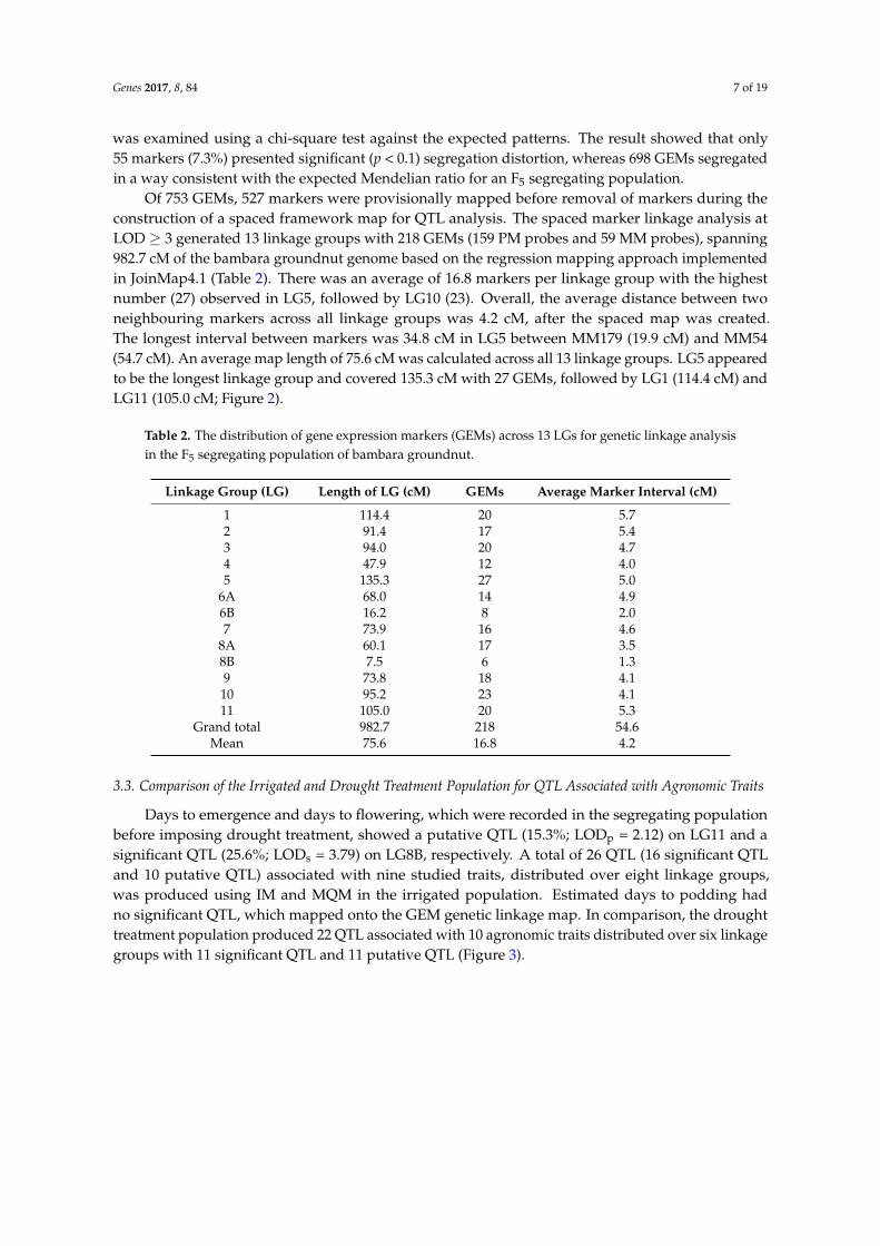
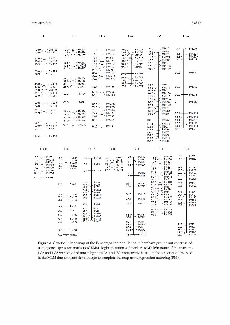
Of 753 GEMs, 527 markers were provisionally mapped before removal of markers during theconstruction of a spaced framework map for QTL analysis. The spaced marker linkage analysis atLOD ≥ 3 generated 13 linkage groups with 218 GEMs (159 PM probes and 59 MM probes), spanning982.7 cM of the bambara groundnut genome based on the regression mapping approach implementedin JoinMap4.1 (Table 2). There was an average of 16.8 markers per linkage group with the highestnumber (27) observed in LG5, followed by LG10 (23). Overall, the average distance between twoneighbouring markers across all linkage groups was 4.2 cM, after the spaced map was created.The longest interval between markers was 34.8 cM in LG5 between MM179 (19.9 cM) and MM54(54.7 cM). An average map length of 75.6 cM was calculated across all 13 linkage groups. LG5 appearedto be the longest linkage group and covered 135.3 cM with 27 GEMs, followed by LG1 (114.4 cM) andLG11 (105.0 cM; Figure 2).

Table 2. The distribution of gene expression markers (GEMs) across 13 LGs for genetic linkage analysisin the F5 segregating population of bambara groundnut.

Linkage Group (LG) Length of LG (cM) GEMs Average Marker Interval (cM)

1 114.4 20 5.72 91.4 17 5.43 94.0 20 4.74 47.9 12 4.05 135.3 27 5.0

6A 68.0 14 4.96B 16.2 8 2.07 73.9 16 4.6

8A 60.1 17 3.58B 7.5 6 1.39 73.8 18 4.1

10 95.2 23 4.111 105.0 20 5.3

Grand total 982.7 218 54.6Mean 75.6 16.8 4.2

3.3. Comparison of the Irrigated and Drought Treatment Population for QTL Associated with Agronomic Traits

Days to emergence and days to flowering, which were recorded in the segregating populationbefore imposing drought treatment, showed a putative QTL (15.3%; LODp = 2.12) on LG11 and asignificant QTL (25.6%; LODs = 3.79) on LG8B, respectively. A total of 26 QTL (16 significant QTLand 10 putative QTL) associated with nine studied traits, distributed over eight linkage groups,was produced using IM and MQM in the irrigated population. Estimated days to podding hadno significant QTL, which mapped onto the GEM genetic linkage map. In comparison, the droughttreatment population produced 22 QTL associated with 10 agronomic traits distributed over six linkagegroups with 11 significant QTL and 11 putative QTL (Figure 3).

Genes 2017, 8, 84 8 of 19Genes 2017, 8, 2 8 of 18

Figure 2. Genetic linkage map of the F5 segregating population in bambara groundnut constructed

using gene expression markers (GEMs). Right: positions of markers (cM); left: name of the markers.

LG6 and LG8 were divided into subgroups ‘A’ and ‘B’, respectively, based on the association observed

in the MLM due to insufficient linkage to complete the map using regression mapping (RM).

Figure 2. Genetic linkage map of the F5 segregating population in bambara groundnut

constructed

Figure 2. Genetic linkage map of the F5 segregating population in bambara groundnut constructedusing gene expression markers (GEMs). Right: positions of markers (cM); left: name of the markers.LG6 and LG8 were divided into subgroups ‘A’ and ‘B’, respectively, based on the association observedin the MLM due to insufficient linkage to complete the map using regression mapping (RM).

Genes 2017, 8, 84 9 of 19Genes 2017, 8, 2 9 of 18

Figure 3. Cont.

Genes 2017, 8, 84 10 of 19Genes 2017, 8, 2 10 of 18

Figure 3. Map positions of the quantitative trait loci (QTL) in the irrigated (control) and drought

treatment F5 segregating population developed from a cross between Tiga Nicuru and DipC. GEMs’

identity is described on the right and map positions (cM) on the left. The rectangular box ( ) with the

solid confidence intervals indicates the location of significant QTL and their flanking markers,

whereas the triangular box (Δ) with dotted confidence intervals represents putative QTL and their

neighbouring markers. DE, days to emergence; DF, days to flowering; EDP, estimated days to

podding; IN, internode length; PEL, peduncle length; PN, pod number per plant; PW, pod weight per

plant; SN, seed number per plant; SW, seed weight per plant; 100SW, 100-seed weight; SDW: shoot

dry weight; HI, harvest index; SC, stomatal conductance; CID, leaf carbon (Delta C13) isotope analysis;

SD, stomatal density; NID, leaf (Delta N15) isotope analysis.

Most of the QTL were clustered, especially on LG1, LG2 and LG11 in the irrigated population.

Of 26 QTL, eight QTL (seven significant QTL and one putative QTL) were located on LG1, whereas

five other QTL were identified on LG2 (two significant QTL and three putative QTL) and six QTL on

LG11 (five significant QTL and one putative QTL). The clusters of QTL in the drought treatment

population were also focused on three linkage groups, with eight QTL on LG1 (five significant QTL

and three putative QTL), four QTL on LG2 (three significant QTL and one putative QTL) and seven

QTL on LG11 (two significant QTL and five putative QTL).

A number of traits are likely to be correlated (Table S1). Some of the QTL have overlapping

confidence intervals, opening up the possibility that they are being influenced by the same underlying

gene. For example, QTL controlling seven traits—internode length, peduncle length, pod number per

plant, seed number per plant, pod weight per plant, seed weight per plant and harvest index—in the

irrigated population were detected at loci closely linked with MM135 (51.8 cM) and PM312

(54.1 cM) on LG1. Specifically, QTL for internode length (42.9%; LODs = 8.72), pod number per plant

(33.9%; LODs = 7.01) and seed number per plant (28.1%; LODs = 6.47) were identified at 52.8 cM, QTL

for peduncle length (41.1%; LODs = 8.93) and pod weight per plant (18.9%; LODs = 4.57) at 53.8 cM

and QTL for seed weight per plant (13.4%; LODs = 3.25) and harvest index (24.5%; LODs = 5.43) at

54.1 cM, although the confidence intervals are all overlapping. The potentially pleiotropic effect of

Figure 3. Map positions of the quantitative trait loci (QTL) in the irrigated (control) and droughttreatment F5 segregating population developed from a cross between Tiga Nicuru and DipC. GEMs’identity is described on the right and map positions (cM) on the left. The rectangular box (

Genes 2017, 8, 2 10 of 18

Figure 3. Map positions of the quantitative trait loci (QTL) in the irrigated (control) and drought treatment F5 segregating population developed from a cross between Tiga Nicuru and DipC. GEMs’ identity is described on the right and map positions (cM) on the left. The rectangular box ( )

with the solid confidence intervals indicates the location of significant QTL and their flanking markers, whereas the triangular box (Δ) with dotted confidence intervals represents putative QTL and their neighbouring markers. DE, days to emergence; DF, days to flowering; EDP, estimated days to podding; IN, internode length; PEL, peduncle length; PN, pod number per plant; PW, pod weight per plant; SN, seed number per plant; SW, seed weight per plant; 100SW, 100-seed weight; SDW: shoot dry weight; HI, harvest index; SC, stomatal conductance; CID, leaf carbon (Delta C13) isotope analysis; SD, stomatal density; NID, leaf (Delta N15) isotope analysis.

Most of the QTL were clustered, especially on LG1, LG2 and LG11 in the irrigated population. Of 26 QTL, eight QTL (seven significant QTL and one putative QTL) were located on LG1, whereas five other QTL were identified on LG2 (two significant QTL and three putative QTL) and six QTL on LG11 (five significant QTL and one putative QTL). The clusters of QTL in the drought treatment population were also focused on three linkage groups, with eight QTL on LG1 (five significant QTL and three putative QTL), four QTL on LG2 (three significant QTL and one putative QTL) and seven QTL on LG11 (two significant QTL and five putative QTL).

A number of traits are likely to be correlated (Table S1). Some of the QTL have overlapping confidence intervals, opening up the possibility that they are being influenced by the same underlying gene. For example, QTL controlling seven traits—internode length, peduncle length, pod number per plant, seed number per plant, pod weight per plant, seed weight per plant and harvest index—in the irrigated population were detected at loci closely linked with MM135 (51.8 cM) and PM312 (54.1 cM) on LG1. Specifically, QTL for internode length (42.9%; LODs = 8.72), pod number per plant (33.9%; LODs = 7.01) and seed number per plant (28.1%; LODs = 6.47) were identified at 52.8 cM, QTL for peduncle length (41.1%; LODs = 8.93) and pod weight per plant (18.9%; LODs = 4.57) at 53.8 cM and QTL for seed weight per plant (13.4%; LODs = 3.25) and harvest index (24.5%; LODs = 5.43) at

) with thesolid confidence intervals indicates the location of significant QTL and their flanking markers, whereasthe triangular box (∆) with dotted confidence intervals represents putative QTL and their neighbouringmarkers. DE, days to emergence; DF, days to flowering; EDP, estimated days to podding; IN, internodelength; PEL, peduncle length; PN, pod number per plant; PW, pod weight per plant; SN, seed numberper plant; SW, seed weight per plant; 100SW, 100-seed weight; SDW: shoot dry weight; HI, harvestindex; SC, stomatal conductance; CID, leaf carbon (Delta C13) isotope analysis; SD, stomatal density;NID, leaf (Delta N15) isotope analysis.

Most of the QTL were clustered, especially on LG1, LG2 and LG11 in the irrigated population.Of 26 QTL, eight QTL (seven significant QTL and one putative QTL) were located on LG1, whereasfive other QTL were identified on LG2 (two significant QTL and three putative QTL) and six QTLon LG11 (five significant QTL and one putative QTL). The clusters of QTL in the drought treatmentpopulation were also focused on three linkage groups, with eight QTL on LG1 (five significant QTLand three putative QTL), four QTL on LG2 (three significant QTL and one putative QTL) and sevenQTL on LG11 (two significant QTL and five putative QTL).

A number of traits are likely to be correlated (Table S1). Some of the QTL have overlappingconfidence intervals, opening up the possibility that they are being influenced by the same underlyinggene. For example, QTL controlling seven traits—internode length, peduncle length, pod number perplant, seed number per plant, pod weight per plant, seed weight per plant and harvest index—in theirrigated population were detected at loci closely linked with MM135 (51.8 cM) and PM312 (54.1 cM)on LG1. Specifically, QTL for internode length (42.9%; LODs = 8.72), pod number per plant (33.9%;LODs = 7.01) and seed number per plant (28.1%; LODs = 6.47) were identified at 52.8 cM, QTL forpeduncle length (41.1%; LODs = 8.93) and pod weight per plant (18.9%; LODs = 4.57) at 53.8 cM

Genes 2017, 8, 84 11 of 19

and QTL for seed weight per plant (13.4%; LODs = 3.25) and harvest index (24.5%; LODs = 5.43) at54.1 cM, although the confidence intervals are all overlapping. The potentially pleiotropic effect ofgenes underlying the QTL could be further observed in QTL located on LG11 at loci closely linkedwith marker MM178 (60.3 cM), such as QTL controlling pod number per plant (13.5%; LODs = 3.15),seed number per plant (15.7%; LODs = 3.82), pod weight per plant (15.1%; LODs = 3.57) and seedweight per plant (16.5%; LODs = 3.99). In addition, the cluster of QTL located at 91.4 cM with linkedmarker MM232 on LG2 consisted of one significant QTL controlling seed weight per plant (13.6%;LODs = 3.39) and one putative QTL controlling pod weight per plant (10.4%; LODp = 2.56) and harvestindex (11.1%; LODp = 2.73).

Some traits were shown to be controlled by multiple loci across different linkage groups.For example, internode length in the irrigated population had significant QTL, which mapped at loci onLG1 and LG8A, which has closely linked markers MM135 (51.8 cM) and PM341 (55.6 cM), respectively,and one putative QTL with marker PM208 (135.3 cM) on LG5. A total of 42.9% of phenotypic variationexplained (PVE) was accounted for (LODs = 8.72) on LG1, followed by 14.5% (LODs = 3.57) on LG8Aand 9.4% (LODp = 2.92) on LG5.

In the drought treatment population, large numbers of QTL clustered on LG1, located in thesame region as the irrigated population between loci with linked markers MM135 and PM312(CI: 51.8 cM–54.1 cM). The observation of overlapping confidence intervals with significant QTLcontrolling several traits in both irrigated and drought treatment population indicates the potential ofintrinsic trait differences between parental genotypes which then segregate in the offspring population.Linkage group LG1 with confidence intervals between 51.8 cM and 54.1 cM were mapped with QTLfor internode length (IR (Irrigated): 42.9%; LODs = 8.72; D (Drought): 40.2%; LODs = 9.06), pedunclelength (IR: 41.1%; LODs = 8.93; D: 54.7%; LODs = 10.83), pod weight per plant (IR: 18.9%; LODs = 4.57;D: 22.8%; LODs = 4.47) and seed number per plant (IR: 28.1%; LODs = 6.47; D: 23.7%; LODs = 3.46)and were consistent across the irrigated and the drought treatment population. In addition, seedweight per plant (IR: 13.6%; LODs = 3.39; D: 19.3%; LODs = 3.16) also overlapped at a location between84.9 cM and 91.4 cM on LG2.

The effect of the drought treatment influencing QTL in the drought treatment population wasidentified for some of the traits. Significant QTL for pod number per plant (33.9%; LODs = 7.01) andharvest index (24.5%; LODs = 5.43) were mapped in an overlapping confidence interval between51.8 cM and 54.1 cM on LG1 in the irrigated population; however, these had been reduced to putativeQTL with reduced phenotypic variation explained (18.2%; LODp = 2.57) and 16.1% (LODp = 2.74)in the drought treatment population, for the respective traits. Further drought treatment modifiedQTL were observed for harvest index in which a significant QTL was mapped on LG2 at 55.3 cM(CI: 53.3 cM–63.6 cM; 17.5%; LODs = 3.00) in the drought treatment population while a putative, butseparate, QTL was mapped at 91.4 cM (CI: 84.9 cM–91.4 cM; 11.1%; LODp = 2.73) on LG2 in theirrigated population. For traits including 100-seed weight and harvest index, mapping of significantQTL on different linkage groups and in different locations on the same linkage group in the droughttreatment population compared to the irrigated population reflected a likely interaction between thedrought treatment and the agronomic traits in the segregating population. For instance, significantQTL for 100-seed weight were mapped on LG2 at 84.0 cM and LG 4 at 16.5 cM in the droughttreatment population, but not in the irrigated treatment, with PVE of 19.1% (LODs = 3.97) and 14.8%(LODs = 3.21), respectively.

3.4. Comparison of the Irrigated and Drought Treatment Population for QTL Associated with Drought

Five traits that have classically been used to evaluate the physiological effects of drought,including stomatal conductance, relative water content, stomatal density, leaf carbon (Delta C13)isotope analysis (CID) and leaf (Delta N15) isotope analysis (NID), were evaluated for QTL, based onthe expression-based (GEM) genetic linkage map (Figure 3). Stomatal density and NID were identifiedto have significant QTL in the irrigated population. QTL controlling stomatal density were identified

Genes 2017, 8, 84 12 of 19

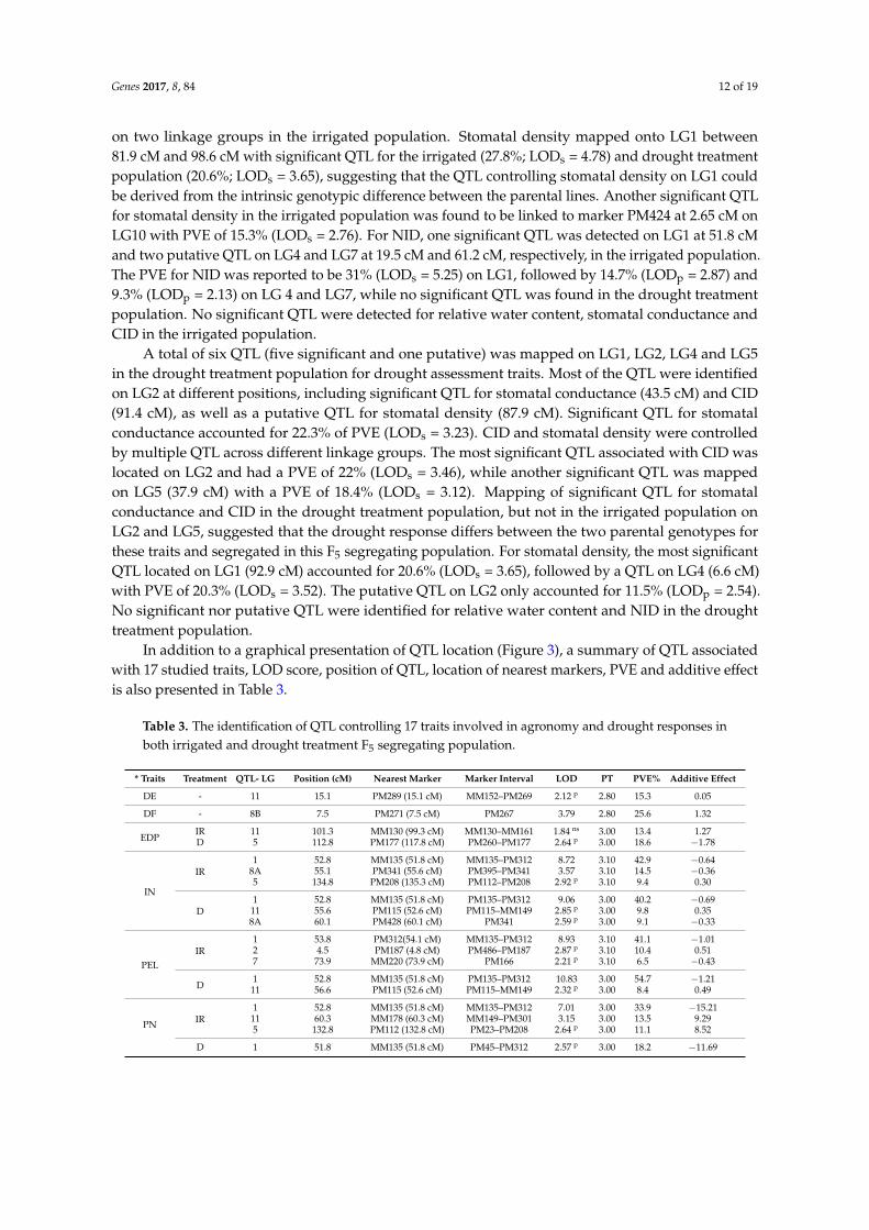
on two linkage groups in the irrigated population. Stomatal density mapped onto LG1 between81.9 cM and 98.6 cM with significant QTL for the irrigated (27.8%; LODs = 4.78) and drought treatmentpopulation (20.6%; LODs = 3.65), suggesting that the QTL controlling stomatal density on LG1 couldbe derived from the intrinsic genotypic difference between the parental lines. Another significant QTLfor stomatal density in the irrigated population was found to be linked to marker PM424 at 2.65 cM onLG10 with PVE of 15.3% (LODs = 2.76). For NID, one significant QTL was detected on LG1 at 51.8 cMand two putative QTL on LG4 and LG7 at 19.5 cM and 61.2 cM, respectively, in the irrigated population.The PVE for NID was reported to be 31% (LODs = 5.25) on LG1, followed by 14.7% (LODp = 2.87) and9.3% (LODp = 2.13) on LG 4 and LG7, while no significant QTL was found in the drought treatmentpopulation. No significant QTL were detected for relative water content, stomatal conductance andCID in the irrigated population.

A total of six QTL (five significant and one putative) was mapped on LG1, LG2, LG4 and LG5in the drought treatment population for drought assessment traits. Most of the QTL were identifiedon LG2 at different positions, including significant QTL for stomatal conductance (43.5 cM) and CID(91.4 cM), as well as a putative QTL for stomatal density (87.9 cM). Significant QTL for stomatalconductance accounted for 22.3% of PVE (LODs = 3.23). CID and stomatal density were controlledby multiple QTL across different linkage groups. The most significant QTL associated with CID waslocated on LG2 and had a PVE of 22% (LODs = 3.46), while another significant QTL was mappedon LG5 (37.9 cM) with a PVE of 18.4% (LODs = 3.12). Mapping of significant QTL for stomatalconductance and CID in the drought treatment population, but not in the irrigated population onLG2 and LG5, suggested that the drought response differs between the two parental genotypes forthese traits and segregated in this F5 segregating population. For stomatal density, the most significantQTL located on LG1 (92.9 cM) accounted for 20.6% (LODs = 3.65), followed by a QTL on LG4 (6.6 cM)with PVE of 20.3% (LODs = 3.52). The putative QTL on LG2 only accounted for 11.5% (LODp = 2.54).No significant nor putative QTL were identified for relative water content and NID in the droughttreatment population.

In addition to a graphical presentation of QTL location (Figure 3), a summary of QTL associatedwith 17 studied traits, LOD score, position of QTL, location of nearest markers, PVE and additive effectis also presented in Table 3.

Table 3. The identification of QTL controlling 17 traits involved in agronomy and drought responses inboth irrigated and drought treatment F5 segregating population.

* Traits Treatment QTL- LG Position (cM) Nearest Marker Marker Interval LOD PT PVE% Additive Effect

DE - 11 15.1 PM289 (15.1 cM) MM152–PM269 2.12 p 2.80 15.3 0.05

DF - 8B 7.5 PM271 (7.5 cM) PM267 3.79 2.80 25.6 1.32

EDPIR 11 101.3 MM130 (99.3 cM) MM130–MM161 1.84 ns 3.00 13.4 1.27D 5 112.8 PM177 (117.8 cM) PM260–PM177 2.64 p 3.00 18.6 −1.78

IN

IR1 52.8 MM135 (51.8 cM) MM135–PM312 8.72 3.10 42.9 −0.64

8A 55.1 PM341 (55.6 cM) PM395–PM341 3.57 3.10 14.5 −0.365 134.8 PM208 (135.3 cM) PM112–PM208 2.92 p 3.10 9.4 0.30

D1 52.8 MM135 (51.8 cM) PM135–PM312 9.06 3.00 40.2 −0.6911 55.6 PM115 (52.6 cM) PM115–MM149 2.85 p 3.00 9.8 0.358A 60.1 PM428 (60.1 cM) PM341 2.59 p 3.00 9.1 −0.33

PELIR

1 53.8 PM312(54.1 cM) MM135–PM312 8.93 3.10 41.1 −1.012 4.5 PM187 (4.8 cM) PM486–PM187 2.87 p 3.10 10.4 0.517 73.9 MM220 (73.9 cM) PM166 2.21 p 3.10 6.5 −0.43

D1 52.8 MM135 (51.8 cM) PM135–PM312 10.83 3.00 54.7 −1.2111 56.6 PM115 (52.6 cM) PM115–MM149 2.32 p 3.00 8.4 0.49

PN IR1 52.8 MM135 (51.8 cM) MM135–PM312 7.01 3.00 33.9 −15.2111 60.3 MM178 (60.3 cM) MM149–PM301 3.15 3.00 13.5 9.295 132.8 PM112 (132.8 cM) PM23–PM208 2.64 p 3.00 11.1 8.52

D 1 51.8 MM135 (51.8 cM) PM45–PM312 2.57 p 3.00 18.2 −11.69

Genes 2017, 8, 84 13 of 19

Table 3. Cont.

* Traits Treatment QTL- LG Position (cM) Nearest Marker Marker Interval LOD PT PVE% Additive Effect

PW

IR1 53.8 MM135 (51.8 cM) MM135–PM312 4.57 3.10 18.9 −10.6011 60.3 MM178 (60.3 cM) MM149–PM301 3.57 3.10 15.1 9.332 91.4 MM232 (91.4 cM) PM340 2.56 p 3.10 10.4 7.83

D1 52.8 MM135 (51.8 cM) PM135–PM312 4.47 3.00 22.8 −10.2611 56.6 MM149 (59.2 cM) PM115–MM149 3.61 3.00 17.5 9.302 58.3 PM190 (53.3 cM) PM190–PM84 2.49 p 3.00 11.1 9.55

SNIR

1 52.8 MM135 (51.8 cM) MM135–PM312 6.47 3.00 28.1 −15.1411 60.3 MM178 (60.3 cM) MM149–PM301 3.82 3.00 15.7 11.062 60.3 PM84 (63.6 cM) PM190–PM84 3.2 3.00 12.4 13.04

D 1 51.8 MM135 (51.8 cM) PM45–PM312 3.46 3.00 23.7 −14.04

SW

IR11 60.3 MM178 (60.3 cM) MM149–PM301 3.99 3.10 16.5 6.972 91.4 MM232 (91.4 cM) PM340 3.39 3.10 13.6 6.411 54.1 PM312(54.1 cM) PM312–PM261 3.25 3.10 13.4 −6.53

D2 91.4 MM232 (91.4 cM) PM340 3.16 3.00 19.3 6.631 51.8 MM135 (51.8 cM) PM45–PM312 2.45 p 3.00 12 −5.3911 55.6 PM115 (52.6 cM) PM115–MM149 2.17 p 3.00 12.5 5.76

100-SW

IR9 52.4 PM181 (55.4 cM) MM238–PM181 4.49 3.00 27.5 −7.6210 21.6 MM131 (22.4 cM) PM98–MM131 2.21 p 3.00 12.7 4.8411 30.2 PM204 (30.2 cM) PM393–MM37 2.38 p 3.00 11.4 4.53

D2 84.0 PM247 (84.0 cM) PM209–PM340 3.97 3.00 19.1 5.534 16.5 MM25 (12.5 cM) MM25–PM164 3.21 3.00 14.8 −5.5211 28.7 PM204 (30.2 cM) PM393–PM204 2.8 p 3.00 12.8 4.62

SDWIR

11 60.2 MM178 (60.3 cM) MM149–MM178 5.62 3.00 27.7 9.738A 56.6 PM341 (55.6 cM) PM341–PM428 2.67 p 3.00 11.3 −6.291 61.0 PM261 (58.0 cM) PM261–PM388 2.28 p 3.00 9.7 −6.18

D1 51.8 MM135 (51.8 cM) PM45–PM312 3.9 2.90 22.4 −8.6311 55.6 PM115 (52.6 cM) PM115–MM149 3.67 2.90 20.2 8.81

HI

IR1 54.1 PM312 (54.1 cM) MM135–PM261 5.43 3.00 24.5 −0.162 91.4 MM232 (91.4 cM) PM340 2.73 p 3.00 11.1 0.11

D2 55.3 PM190 (53.3 cM) PM190–PM84 3 3.00 17.5 0.121 52.8 MM135 (51.8 cM) PM135–PM312 2.74 p 3.00 16.1 −0.1011 27.7 PM204 (30.2 cM) PM393–PM204 2.2 p 2.80 10.6 0.09

RWCIR 10 2.1 PM136 (2.1 cM) MM197–PM424 1.86 ns 2.90 13.5 0.58D 5 0.0 MM89 (0.0 cM) MM82 1.35 ns 3.00 10 0.38

SCIR 3 24.7 PM103 (24.7cM) MM56–MM235 1.17 ns 2.60 8.7 15.83D 2 43.5 MM61 (42.5 cM) MM61–PM190 3.23 3.00 22.3 17.76

CID

IR 3 8.9 PM327 (4.6 cM) PM327–PM211 1.63 ns 3.00 12.5 0.46

D5 37.9 MM54 (54.7 cM) MM179–MM54 3.23 3.00 18.4 −0.602 91.4 MM232 (91.4 cM) PM340 3.46 3.00 22 −0.43

SD

IR1 87.9 PM96 (81.9 cM) PM96–PM213 4.78 2.50 27.3 2.2510 2.7 PM424 (2.7 cM) PM136–PM191 2.76 2.50 15.3 −1.41

D1 92.9 PM213 (98.6 cM) PM96–PM213 3.65 3.00 20.6 1.434 6.6 PM372 (6.6 cM) PM315–PM422 3.52 3.00 20.3 1.232 87.9 MM232 (91.4 cM) PM340–MM232 2.54 p 3.00 11.5 −0.98

NIDIR

1 51.8 MM135 (51.8 cM) PM45–PM312 5.25 3.00 31 −0.464 19.5 MM25 (12.5 cM) MM25–PM164 2.87 p 3.00 14.7 0.397 61.2 PM378 (61.7 cM) PM298–PM378 2.13 p 3.00 9.3 −0.27

D 11 51.1 PM83 (51.1 cM) PM389–PM52 1.64 ns 3.00 12.4 −0.28

ns: non-significance at p ≤ 0.05 by the permutation test using 10,000 reiterations. p: putative QTL where theLOD score is lower than the GW threshold by up to a 1-LOD interval. PT: permutation test threshold using10,000 reiterations at p ≤ 0.05. * DE, days to emergence; DF, days to flowering; EDP, estimated days to podding;IN, internode length; PEL, peduncle length; PN, pod number per plant; PW, pod weight per plant; SN, seednumber per plant; SW, seed weight per plant; 100-SW, 100-seed weight; SDW: shoot dry weight; HI, harvest index;SC, stomatal conductance; CID, leaf carbon (Delta C13) isotope analysis; SD, stomatal density; NID, leaf (Delta N15)isotope analysis.

4. Discussion

4.1. Novel GEMs Generated Using Affymetrix Soybean Genome GeneChip

The use of a microarray offers the potential to obtain both gene expression variation(pseudo-phenotypic data) and genotypic markers for the construction of a genetic linkage map,allowing the identification of thousands of markers in a single experiment. When integrated withtrait QTL, the causal loci within the QTL genomic regions and the hypothetical regulatory networkscontrolling phenotypic variation could, potentially, be analysed. Despite the transcriptome sequence

Genes 2017, 8, 84 14 of 19

information for bambara groundnut not being fully available and the lack of a genome sequence,the development of a novel mapping marker system through cross-hybridising bambara groundnutRNA onto the Affymetrix Soybean Genome GeneChip allowed the construction of a high densityexpression-based genetic map for bambara groundnut with subsequent trait QTL analysis, as well aspermitting a comparison of the genomic location of the detected genetic effects in bambara groundnut(QTL) with the equivalent genomic locations in soybean. An example of using cross-species approachesto translate genomic resources from model plants to a less intensively studied plants was reported incowpea [18]. A total of 1058 single feature polymorphism (SFPs), which are microarray-based markers,were detected and validated in cowpea using Affymetrix Soybean Genome GeneChip, enablingsubsequent high-throughput genotyping and high density mapping in cowpea [18].

In previous publications, the development of GEMs is based on the average hybridisation signalproduced from a single probe-set, which is represented by ~11 probe-pairs when the AffymetrixGeneChip is used or by a number of features when an Agilent chip is used (usually 1–3 60-merprobes). The first approach in which the hybridisation signal was measured at the level of thesoybean probe-sets identified 15 (0.02%) potential GEMs out of 61,035 probe-sets, and this may bedue to the hybridisation of RNA samples from bambara groundnut onto a heterologous soybeangenome microarray (evolutionary separation of the two species being around 20 million years; [27]).Despite reasonably high signal strength that might be generated by one probe-pair in a probe-set, thehybridisation signal is averaged across all probe-pairs that represent that probe-set. Poor hybridisationto other probe-pairs could reduce the overall mean, and as a result, a relatively low distinctness scorecould be produced, resulting in few GEMs being selected. The results improved when probe-setswere masked with a custom made CDF file to remove probe-pairs with poor hybridisation signal.Forty-eight genes out of 53,651 (0.09%) were selected as GEMs.

However, the number of GEMs generated at probe-set (15) and CDF masked probe-set level(48) was insufficient for use in genetic linkage analysis as a single marker type. The developmentof GEMs at the probe-pair level was established to overcome the likely signal damping effectresulting from averaging of the signal across all probe-pairs in each probe-set. From the list ofprobe-pairs with different distinctness scores, differential hybridisation to the probe-pairs from thesame probe set was also discovered, for example: Gma.12360.1.S1_at; PM-394638, Gma.12360.1.S1_at;PM-1346833 and Gma.12360.1.S1_at; PM-432117, which showed distinctness scores of 3.72, 2.08 and1.73, respectively. The analysis of the hybridisation signal data at the probe-pair level offers anadvantage in terms of retrieving potential probe-pairs with a high distinctness score and to removepoorly-hybridised probe-pairs from each probe-set in order to obtain as much information as possiblefor GEMs’ development.

Of 669,982 probes, 1029 PM probes and 501 MM probes (0.23%) were chosen as potential GEMswhen the analysis was conducted at the probe-pair level. A similar number of GEMs were used for mapconstruction (838 putative GEMs out of 92 k transcripts from the Agilent Brassica 60-mer array; [14]).The current cross-species analysis has not only to contend with the small number of genes actuallyshowing a DNA-based (sequence) or RNA-based (expression level) difference during a homologousspecies-chip analysis, but must also contend with lower signal strength due to evolutionary distancebetween target species and the microarray used.

A distinctness score was used to enrich for the separation of ‘a’ and ‘b’ allele scores across theindividual lines, allowing the probe-pairs to be selected as potential GEMs. A high distinctness scoreshould distinguish between ‘a’ and ‘b’ allele across individual lines and assign them, largely, intotwo distinct groups. For example, Gma.15877.1.S1_at; PM-41730, with a distinctness score of 5.31produced two distinct groups that showed hybridisation signal as high as 2360.75 (‘a’ allele, average:1938.53; s.d.: 218.97) and as low as 256.44, respectively (‘b’ allele, average: 395.16; s.d.: 80.63). The mostlikely explanation of such large differences would be the accidental sequence homology of a repetitiveelement present in one genotype, but not the other. For the associated GEM to map would requirethat the repetitive sequence were randomly repeated at only a single locus. For decreased values of

Genes 2017, 8, 84 15 of 19

the distinctness score, the distribution of the two allele groups becomes more scattered, and thereis the potential of having a hybridisation signal from some individual lines falling in between thetwo distinct groups, for instance GmaAffx.71175.1.S1_s_at; PM-1195578 with a distinctness score of3.82. This noise could be due to technical issues, such as the strength of the hybridisation of nucleicacids onto an individual GeneChip (although all chips were normalised before analysis) and risksmisclassification of allele types. Thus, a series of cut-off points are set during data analysis in order toremove probe-pairs with poor performance, very similar signal or with high scatter across lines. It isalso worth noting that the current cross is at the F5 generation, so 1/16th heterozygosity would bepredicted to remain in the lines, per marker, on average (6.25%), and 3–4 individuals in the populationmight be expected to be heterozygous for any marker. If the markers behave in a co-dominant (dosagedependent) way, then there are likely to be a number of intermediate a/b markers, which wouldreduce the distinctness score and could lead to marker rejection.

4.2. Use of GEMs for Genetic Mapping

In terms of quantity, the use of both PM probes and MM probes increases the number of markersavailable for genetic mapping. The spaced framework genetic map, which was produced afterrepetitive rounds of removing markers, is expected to represent the most robust markers withreasonable overall coverage for the F5 segregating population of 65 individual lines in bambaragroundnut. The PM probes and MM probes in each probe-pair could have different hybridisationsignals due to the single nucleotide difference present by the design at the 13th nucleotide between thePM and MM probe of a probe-pair. This could result in a variation of the distinctness score and mightgive some indication of the basis of the polymorphism mapped.

The first priority in map construction must be to use the best quality data to produce the mostaccurate map, then additional putative markers could be introduced using less stringent criteria, butfixing the order of the framework map first. If the data quality is good, additional markers will allowdenser maps to be constructed. If the additional marker quality is poor, approximate positions can stillbe assigned, which could be useful in any conserved synteny comparisons or subsequent fine mapping.

As GEMs are potentially ‘transient’ markers, the integration of GEMs into a stable DNAsequence-based framework map is recommended [12]. There are several potential advantages for theintegration of maps. Integration of maps allows the potential alignment of GEMs and thus also theDNA sequence-based framework map to the soybean physical map. A detailed integrated map inbambara groundnut would be necessary in future to offer greater potential to map QTL with traits ofinterest more accurately.

4.3. Association between Markers and Traits in Bambara Groundnut

A similar pattern of QTL controlling the studied common traits in both irrigated and droughttreatment populations suggested that most of the detected QTL are the result of intrinsic differencesbetween the parental lines used to create the segregating population, with limited responses tothe imposed drought. Several QTL were found to effect internode length and peduncle length inboth drought and irrigated populations with the significant QTL consistently mapped to LG1 in thesegregating population across the two treatments. However, there were minor QTL effecting internodelength, such as QTL in LG8A, which explained 14.5% (LODs = 3.57) and 9.1% (LODp =2.59) in theirrigated population and drought treatment population, respectively. The inheritance of internodelength was contributed to by one major QTL plus a few minor QTL. The major QTL linked with thesame marker on LG1 suggested that these two traits are probably largely controlled by a single gene ortwo closely-linked genes. The hypothesis may be supported by Basu et al. (2007) [8] who reported thatthe segregation pattern of internode length was consistent with primarily monogenic inheritance in adomesticated (DipC) line crossed with a V. subterranea var. spontanea (VSSP11), created to evaluate thedomestication process in bambara groundnut. This detected locus could represent residual variationat the same gene whose domestication led to the bunchy morphology.

Genes 2017, 8, 84 16 of 19

The present study showed the potential interaction of complex traits, such as pod number perplant and 100-seed weight, with environmental factors (such as drought) and underlying the genescontrolling yield traits, given that they are downstream traits. The discovery of a number of QTL (ratherthan a single major locus) explaining more limited phenotypic variation for yield traits suggested thatthese traits could probably be controlled by many genes with minor effects, as has been generallyreported for yield. For instance, 100-seed weight was contributed to by multiple loci located acrossLG2, LG4 and LG11, explaining 19.1%, 14.8% and 12.8% of the phenotypic variation, respectively, inthe drought treatment population. The observation of multiple genes with minor effects controllingyield-related traits was also reported by Zhang et al. (2004) [28] who discovered four QTL located onthree linkage groups (A2, B1 and D2) for seed weight in RILs derived from soybean vars. Kefeng No.1X Nannong 1138-2.

The present study also showed that QTL controlling internode length, peduncle length, podnumber per plant and seed number per plant were linked with the same marker MM135 at 51.8 cMon LG1. The clustered QTL on LG1 could correspond to a single gene controlling plant architecture,which has pleiotropic effects on different traits, including seed and plant growth-related traits. In pea,QTL detected for seed traits were found to be located in the genomic regions regulating traits, such asplant morphology, phenology and plant biomass [22]. The authors showed that the Le allele, whichis related to internode length, has pleiotropic effects on other traits, such as plant height, vegetativebiomass and plant nitrogen content. In wheat, the dwarfism gene (Rht-1) is associated with manyQTL, including grain yield and root development QTL [29]. In rice, a single gene controlling erect leafdevelopment is associated with higher grain yield [30].

For drought-related traits, QTL for stomatal conductance, carbon isotope discrimination analysisand stomatal density were largely located on LG2 in the drought treatment population. Mild droughttreatment was expected to activate gene expression in bambara groundnut in response to stress, leadingto identification of response-associated QTL, specifically in the drought treatment population only.The location of QTL for NID was detected in irrigated plants on LG1 (51.8 cM; CI: 47.5 cM–54.1 cM),corresponding to loci that linked with internode length, pod number per plant, pod weight perplant and seed number per plant (CI: 47.5 cM–54.1 cM). The co-located QTL illustrate the positiverelationship between nitrogen assimilation and biomass in plants. Coque et al. (2006) [31] reportedthat twelve QTL mapped with 15N abundance were involved in nitrogen use efficiency, such as grainyield, N uptake and N remobilisation. However, the non-significant QTL for NID in drought treatmentplants could be explained by the effect of mild drought imposed on the plants and potential limitationsto uptake of N (given that it is water soluble) and reduced biomass production, resulting in a relativelyweak association between loci and traits.

The application of QTL analysis can be extended to the identification of candidate genesthat control these respective traits. An example of using cross-species approaches to identifycandidate genes is reported in cowpea. Through the syntenic relationship between cowpea withMedicago truncatula and soybean, the syntenic locus for Hls (hastate leaf shape) was discoveredand led to the identification of a candidate gene controlling leaf morphology in cowpea [32].The cross-species approach presented in cowpea provides an alternative option to identify candidategenes in underutilised crop species.

5. Conclusions

This study produced GEMs at the (unmasked) probe-pair (oligonucleotide) level aftercross-hybridising leaf RNA from a segregating bambara groundnut cross under a mild droughttreatment with the Affymetrix Soybean Genome GeneChip. This is the first development of GEMs inbambara groundnut, and they are expected to represent either differences in the hybridisation signalof RNA to individual oligonucleotide probes or genuine differences in gene expression levels. A firstspaced GEM map was then developed, and this is also the first ‘expression-based’ map in bambaragroundnut. The first comprehensive QTL analysis with good genome coverage using the GEM map

Genes 2017, 8, 84 17 of 19

showed the usefulness of the GEM map in mapping both intrinsic and drought-related QTL in theF5 segregating population. This study also serves as a starting point for fine mapping, which allowstargeted QTL identification for further application in marker-assisted selection within this minorlegume crop, which already has good drought tolerance characteristics. That QTL were discoveredrelating to stomatal conductance, carbon isotope discrimination analysis and stomatal density of thedrought assessment traits suggests that the two parental lines do differ in their response to drought,and a more detailed analysis may allow these mechanisms to be elucidated.

Supplementary Materials: The following are available online at www.mdpi.com/2073-4425/8/2/84/s1:Supplemental Text S1: Generations of GEMs; Table S1: Pearson’s Correlation Coefficients between agronomictraits measured in both irrigated and drought treatment F5 segregating population.

Acknowledgments: This study was supported by the University of Nottingham Malaysia Campus under MalaysiaIntercampus Doctoral Award Scheme (MIDAS).

Author Contributions: Hui Hui Chai performed the experiments, analysed the data, interpreted the results andwrote the manuscript. Wai Kuan Ho co-analysed the data and interpreted the results. Neil Graham conductedmicroarray data analysis. Sean May developed the idea of cross-species microarray approach. Festo Massawedeveloped the project and critically reviewed the manuscript. Sean Mayes developed the project, co-analysed thedata, interpreted the results and critically reviewed the manuscript.

Conflicts of Interest: The authors declare no conflict of interest. The founding sponsors had no role in the designof the study; in the collection, analyses or interpretation of data; in the writing of the manuscript; nor in thedecision to publish the results.

References

1. Sellschope, J.P.F. Cowpeas, Vigna unguiculata (L.) walp. Field Crops Res. 1962, 15, 259–266.2. Brough, S.H.; Azam-Ali, S.N. The effect of soil moisture on the proximate composition of Bambara groundnut

(Vigna subterranea (L.) Verdc). J. Sci. Food Agric. 1992, 60, 197–203. [CrossRef]3. Heller, J.; Begemann, F.; Mushonga, J. Bambara groundnut (Vigna subterranea (L.) Verdc.). In Promoting the

Conservation and Use of Underutilized and Neglected Crops, 9, Proceedings of the Workshop on Conservation andImprovement of Bambara Groundnut (Vigna subterranea (L.) Verdc), Harare, Zimbabwe, 14–16 November 1995;International Plant Genetic Resources Institute (IPGRI): Rome, Italy.

4. Mukurumbira, L.W. Effects of the rate of fertiliser nitrogen and the previous grain legume on maize yields.Zimbabwe J. Agric. Res. 1985, 82, 177–179.

5. Massawe, F.J.; Mwale, S.S.; Azam-Ali, S.N.; Roberts, J.A. Breeding in Bambara groundnut (Vigna subterranea(L.) Verdc.): Strategic considerations. Afr. J. Biotechnol. 2005, 4, 463–471.

6. Molosiwa, O.O.; Aliyu, S.; Stadler, F.; Mayes, K.; Massawe, F.; Killian, A.; Mayes, S. SSR marker development,genetic diversity and population structure analysis of bambara groundnut [Vigna subterranea (L.) Verdc.]landraces. Genet. Resour. Crop Evol. 2015, 62, 1225–1243. [CrossRef]

7. Basu, S.; Roberts, J.A.; Azam-Ali, S.N.; Mayes, S. Bambara groundnut. In Genome Mapping and MolecularBreeding in Plants—Pulses, Sugar and Tuber; Kole, C.M., Ed.; Springer: New York, NY, USA, 2007; pp. 159–173.

8. Basu, S.; Mayes, S.; Davey, M.; Roberts, J.A.; Azam-Ali, S.N.; Mithen, R.; Pasquet, R.S. Inheritance of‘domestication’ traits in Bambara groundnut (Vigna subterranea (L.: Verdc.). Euphytica 2007, 157, 59–68.[CrossRef]

9. Ahmad, N.S.; Redjeki, E.S.; Ho, W.K.; Aliyu, S.; Mayes, K.; Massawe, F.; Killian, A.; Mayes, S. Constructionof a genetic linkage map and QTL analysis in Bambara groundnut. Genome 2016, 59, 459–472. [CrossRef][PubMed]

10. Winzeler, E.A.; Richards, D.R.; Conway, A.R.; Goldstein, A.L.; Kalman, S.; McCullough, M.J.; McCusker, J.H.;Stevens, D.A.; Wodicka, L.; Lockhart, D.J.; et al. Direct allelic variation scanning of the yeast genome. Science1998, 281, 1194–1197. [CrossRef] [PubMed]

11. Ronald, J.; Akey, J.M.; Whittle, J.; Smith, E.N.; Yvert, G.; Kruglyak, L. Simultaneous genotyping,gene-expression measurement, and detection of allele-specific expression with oligonucleotide arrays.Genome Res. 2005, 15, 284–291. [CrossRef] [PubMed]

Genes 2017, 8, 84 18 of 19

12. West, M.A.L.; van Leeuwen, H.; Kozik, A.; Kliebenstein, D.J.; Doerge, R.W.; St Clair, D.A.; Michelmore, R.W.High-density haplotyping with microarray-based expression and single feature polymorphism markers inArabidopsis. Genome Res. 2006, 16, 787–795. [CrossRef] [PubMed]

13. Potokina, E.; Druka, A.; Luo, Z.W.; Wise, R.; Waugh, R.; Kearsey, M.J. eQTL analysis of 16,000 barley genesreveals a complex pattern of genome wide transcriptional regulation. Plant J. 2007, 53, 90–101. [CrossRef][PubMed]

14. Hammond, J.P.; Mayes, S.; Bowen, H.C.; Graham, N.S.; Hayden, R.M.; Love, C.G.; Spracklen, W.P.; Wang, J.;Welham, S.J.; White, P.J.; et al. Regulatory hotspots are associated with plant gene expression under varyingsoil phosphorus supply in Brassica rapa. Plant Physiol. 2011, 156, 1230–1241. [CrossRef] [PubMed]

15. Hammond, J.P.; Broadley, M.R.; Craigon, D.J.; Higgins, J.; Emmerson, Z.F.; Townsend, H.J.; White, P.J.;May, S.T. Using genomic DNA-based probe-selection to improve the sensitivity of high-densityoligonucleotide arrays when applied to heterologous species. Plant Methods 2005, 1, 1–10. [CrossRef][PubMed]

16. Affymetrix. Available online: http://www.affymetrix.com/estore/ (accessed on 17 October 2016).17. Peng, J.R.; Richards, D.E.; Hartley, N.M.; Murphy, G.P.; Devos, K.M.; Flintham, J.E.; Beales, J.; Fish, L.J.;

Worland, A.J.; Pelica, F.; et al. ‘Green revolution’ genes encode mutant gibberellin response modulators.Nature 1999, 400, 256–261. [PubMed]

18. Das, S.; Bhat, P.R.; Sudhakar, C.; Ehlers, J.D.; Wanamaker, S.; Roberts, P.Q.; Cui, X.P.; Close, T.J. Detection andvalidation of single feature polymorphisms in cowpea (Vigna unguiculata L. Walp) using a soybean genomearray. BMC Genomics 2008, 9, 1–12. [CrossRef] [PubMed]

19. Davey, M.W.; Graham, N.S.; Vanholme, B.; Swennen, R.; May, S.T.; Keulemans, J. Heterologousoligonucleotide microarrays for transcriptomics in a non-model species; a proof-of-concept study of droughtstress in Musa. BMC Genomics 2009, 10, 1–19. [CrossRef] [PubMed]

20. Calvino, M.; Miclaus, M.; Bruggmann, R.; Messing, J. Molecular markers for sweet sorghum based onmicroarray expression data. Rice 2009, 2, 129–142. [CrossRef]

21. Die, J.V.; Rowland, L.J. Superior Cross-Species Reference Genes: A Blueberry Case Study. PLoS ONE 2013, 8,e73354. [CrossRef] [PubMed]

22. Burstin, J.; Marget, P.; Huart, M.; Moessner, A.; Mangin, B.; Duchene, C.; Desprez, B.; Munier-Jolain, N.;Duc, G. Developmental genes have pleiotropic effects on plant morphology and source capacity, eventuallyimpacting on seed protein content and productivity in pea. Plant Physiol. 2007, 144, 768–781. [CrossRef][PubMed]

23. Foucher, F.; Morin, J.; Courtiade, J.; Cadioux, S.; Ellis, N.; Banfield, M.J.; Rameau, C. Determine and lateflowering is two Terminal FLOWER1/CENTRORADIALIS homologs that control two distinct phases offlowering initiation and development in pea. Plant Cell 2003, 15, 2742–2754. [CrossRef] [PubMed]

24. Chai, H.H.; Massawe, F.; Mayes, S. Effects of mild drought stress on the morpho-physiological characteristicsof a Bambara groundnut segregating population. Euphytica 2016, 208, 225–236. [CrossRef]

25. Lai, H.M.; May, S.T.; Mayes, S. Pigeons: A novel GUI software for analysing and parsing high densityheterologous oligonucleotide microarray probe level data. Microarrays 2014, 3, 1–23. [CrossRef] [PubMed]

26. Van Ooijen, J.W. JoinMap 4, Software for the Calculation of Genetic Linkage Maps in Experimental Populations;Kyazma B. V: Wageningen, The Netherlands, 2006.

27. Cannon, S.B.; Gregory, D.M.; Jackson, S.A. Three sequenced legume genomes and many crop species: Richopportunities for translational genomics. Plant Physiol. 2009, 151, 970–977. [CrossRef] [PubMed]

28. Zhang, W.K.; Wang, Y.J.; Luo, G.Z.; Zhang, J.S.; He, C.Y.; Wu, X.L.; Gai, J.Y.; Chen, S.Y. QTL mapping of tenagronomic traits on the soybean (Glycine max L. Merr.) genetic map and their association with EST markers.Theor. Appl. Genet. 2004, 108, 1131–1139. [CrossRef] [PubMed]

29. Laperche, A.; Devienne-Barret, F.; Maury, O.; Le Gouis, J.; Ney, B. A simplified conceptual model ofcarbon/nitrogen functioning for QTL analysis of winter wheat adaptation to nitrogen deficiency. Theor. Appl.Genet. 2006, 113, 1131–1146. [CrossRef] [PubMed]

30. Sakamoto, T.; Morinka, Y.; Ohnishi, T.; Sunohara, H.; Fujioka, S.; Ueguchi-Tanaka, M.; Mizutani, M.;Sakata, K.; Takatsuto, S.; Yoshida, S.; et al. Erect leaves caused by brassinosteroid deficiency increase biomassproduction and grain yield in rice. Nat. Biotechnol. 2006, 24, 105–109. [CrossRef] [PubMed]

Genes 2017, 8, 84 19 of 19

31. Coque, M.; Bertin, P.; Hirel, B.; Gallais, A. Genetic variation and QTL for 15N natural abundance in a set ofmaize recombinant inbred lines. Field Crops Res. 2006, 97, 310–321. [CrossRef]

32. Pottorff, M.; Ehlers, J.D.; Fatokun, C.; Roberts, P.A.; Close, T.J. Leaf morphology in Cowpea [Vigna unguiculata(L.) Walp]: QTL analysis, physical mapping and identifying a candidate gene using synteny with modellegume species. Genomics 2012, 13, 234–245. [CrossRef] [PubMed]

© 2017 by the authors. Licensee MDPI, Basel, Switzerland. This article is an open accessarticle distributed under the terms and conditions of the Creative Commons Attribution(CC BY) license (http://creativecommons.org/licenses/by/4.0/).