a data-driven block thresholding approach to …hz68/sureblock.pdfa data-driven block thresholding...

The Annals of Statistics2009, Vol. 37, No. 2, 569–595DOI: 10.1214/07-AOS538© Institute of Mathematical Statistics, 2009

A DATA-DRIVEN BLOCK THRESHOLDING APPROACH TOWAVELET ESTIMATION

BY T. TONY CAI1 AND HARRISON H. ZHOU2

University of Pennsylvania and Yale University

A data-driven block thresholding procedure for wavelet regression is pro-posed and its theoretical and numerical properties are investigated. The proce-dure empirically chooses the block size and threshold level at each resolutionlevel by minimizing Stein’s unbiased risk estimate. The estimator is sharpadaptive over a class of Besov bodies and achieves simultaneously within asmall constant factor of the minimax risk over a wide collection of BesovBodies including both the “dense” and “sparse” cases. The procedure is easyto implement. Numerical results show that it has superior finite sample per-formance in comparison to the other leading wavelet thresholding estimators.

1. Introduction. Consider the nonparametric regression model

yi = f (ti) + σzi, i = 1,2, . . . , n,(1)

where ti = i/n, σ is the noise level and zi’s are independent standard normalvariables. The goal is to estimate the unknown regression function f (·) based onthe sample {yi}.

Wavelet methods have demonstrated considerable success in nonparametric re-gression. They achieve a high degree of adaptivity through thresholding of the em-pirical wavelet coefficients. Standard wavelet approaches threshold the empiricalcoefficients term by term based on their individual magnitudes. See, for example,Donoho and Johnstone (1994a), Gao (1998) and Antoniadis and Fan (2001). Morerecent work has demonstrated that block thresholding, which simultaneously keepsor kills all the coefficients in groups rather than individually, enjoys a number ofadvantages over the conventional term-by-term thresholding. Block thresholdingincreases estimation precision by utilizing information about neighboring waveletcoefficients and allows the balance between variance and bias to be varied alongthe curve which results in adaptive smoothing. The degree of adaptivity, however,depends on the choice of block size and threshold level.

The idea of block thresholding can be traced back to Efromovich (1985) inorthogonal series estimators. In the context of wavelet estimation, global level-by-level thresholding was discussed in Donoho and Johnstone (1995) for regression

Received November 2006.1Supported in part by NSF Grants DMS-03-06576 and DMS-06-04954.2Supported in part by NSF Grant DMS-06-45676.AMS 2000 subject classifications. Primary 62G08; secondary 62G20.Key words and phrases. Adaptivity, Besov body, block thresholding, James–Stein estimator, non-

parametric regression, Stein’s unbiased risk estimate, wavelets.

569

http://www.imstat.org/aos/

http://dx.doi.org/10.1214/07-AOS538

http://www.imstat.org

http://www.ams.org/msc/

570 T. T. CAI AND H. H. ZHOU

and in Kerkyacharian, Picard and Tribouley (1996) for density estimation. Butthese block thresholding methods are not local, so they do not enjoy a high degreeof spatial adaptivity. Hall, Kerkyacharian and Picard (1999) introduced a localblockwise hard thresholding procedure for density estimation with a block size ofthe order (logn)2 where n is the sample size. Cai (1991) considered blockwiseJames–Stein rules and investigated the effect of block size and threshold level onadaptivity using an oracle inequality approach. In particular it was shown that ablock size of order logn is optimal in the sense that it leads to an estimator whichis both globally and locally adaptive. Cai and Silverman (2001) considered over-lapping block thresholding estimators and Chicken and Cai (2005) applied blockthresholding to density estimation.

The block size and threshold level play important roles in the performance ofa block thresholding estimator. The local block thresholding methods mentionedabove all have fixed block size and threshold and same thresholding rule is appliedto all resolution levels regardless of the distribution of the wavelet coefficients. Inthe present paper, we propose a data-driven approach to empirically select both theblock size and threshold at individual resolution levels. At each resolution level, theprocedure, SureBlock, chooses the block size and threshold by minimizing Stein’sUnbiased Risk Estimate (SURE). By empirically selecting both the block size andthreshold and allowing them to vary from resolution level to resolution level, Sure-Block has significant advantages over the more conventional wavelet thresholdingestimators with fixed block sizes.

Both the numerical performance and asymptotic properties of SureBlock arestudied in this paper. The SureBlock estimator is completely data-driven and easyto implement. A simulation study is carried out and the numerical results showthat SureBlock has superior finite sample performance in comparison to the otherleading wavelet estimators. More specifically, SureBlock uniformly outperformsboth VisuShrink and SureShrink [Donoho and Johnstone (1994a, 1995)] in all 42simulation cases in terms of the average squared error. SureBlock procedure isbetter than BlockJS [Cai (1991)] in 37 out of 42 cases.

The theoretical properties of SureBlock are considered in the Besov space for-mulation, that is, by now classical for the analysis of wavelet methods. Besovspaces, denoted by Bα

p,q and defined in Section 5, are a very rich class of functionspaces which contain functions of inhomogeneous smoothness. The theoretical re-sults show that SureBlock automatically adapts to the sparsity of the underlyingwavelet coefficient sequence and enjoys excellent adaptivity over a wide range ofBesov bodies. In particular, in the “dense case” p ≥ 2 the SureBlock estimatoris sharp adaptive over all Besov bodies Bα

p,q(M) with p = q = 2 and adaptivelyachieves within a factor of 1.25 of the minimax risk over Besov bodies Bα

p,q(M)

for all p ≥ 2, q ≥ 2. At the same time the SureBlock estimator achieves simultane-ously within a constant factor of the minimax risk over a wide collection of Besovbodies Bα

p,q(M) in the “sparse case” p < 2. These properties are not shared simul-taneously by many commonly used fixed block size procedures such as VisuShrink

DATA-DRIVEN BLOCK THRESHOLDING APPROACH 571

[Donoho and Johnstone (1994a)], SureShrink [Donoho and Johnstone (1995)] orBlockJS [Cai (1991)].

The paper is organized as follows. In Section 2 we introduce the SureBlockmethod for the multivariate normal mean problem and derive oracle inequalitiesfor the SureBlock estimator. The results developed in this section provide motiva-tions and necessary technical tools for SureBlock in the wavelet regression setting.In Section 3, after a brief review of wavelets, the SureBlock procedure for the non-parametric regression is proposed. Section 4 discusses numerical implementationand compares the numerical performance of SureBlock with those of VisuShrink[Donoho and Johnstone (1994a)], SureShrink [Donoho and Johnstone (1995)] andBlockJS [Cai (1991)]. Asymptotic properties of the SureBlock estimator are pre-sented in Section 5. The proofs are given in Section 6.

2. Estimation of a normal mean. As mentioned in the Introduction, throughan orthogonal discrete wavelet transform (DWT) the nonparametric regressionproblem can be turned into a problem of estimating the wavelet coefficients at indi-vidual resolution levels. The function estimation procedure as well as the analysisof the estimator become clear once the problem of estimating the wavelet coeffi-cients at a given resolution level is well understood. In this section we shall treatthe estimation problem at a single resolution level by considering a more genericproblem, that of estimating the mean of a multivariate normal variable.

Suppose that we observe

xi = θi + zi, zii.i.d.∼ N(0,1), i = 1,2, . . . , d,(2)

and wish to estimate the mean vector θ = (θ1, . . . , θd) based on the observationsx = (x1, . . . , xd) under the average mean squared error

R(θ, θ) = d−1d∑

i=1

E(θi − θi)2.(3)

This normal mean problem occupies a central position in statistical estimation the-ory. Many methods have been introduced in the literature. In this section, with theapplication to wavelet function estimation in mind, we estimate the mean θ by ablockwise James–Stein estimator with block size L and threshold level λ chosenempirically by minimizing SURE. Oracle inequalities are developed in Section 2.2.

2.1. SureBlock Procedure. A block thresholding procedure thresholds the ob-servations in groups and makes simultaneous decisions on all the means withina block. Let L ≥ 1 be the possible length of each block, and m = d/L be the num-ber of blocks. (For simplicity we shall assume that d is divisible by L in thefollowing discussion.) Fix a block size L and a threshold level λ and divide theobservations x1, x2, . . . , xd into blocks of size L. Let xb = (x(b−1)L+1, . . . , xbL)

represent observations in the bth block, and similarly θb = (θ(b−1)L+1, . . . , θbL)


and zb = (z(b−1)L+1, . . . , zbL). Let S2b = ‖xb‖2

2 for b = 1,2, . . . ,m. The block-wise James–Stein estimator is given by

θ b(λ,L) =(

1 − λ

S2b

)+xb, b = 1,2, . . . ,m,(4)

where λ ≥ 0 is the threshold level. Block thresholding estimators depend on thechoice of the block size L and threshold level λ which largely determines theperformance of the resulting estimator. It is thus important to choose L and λ inan optimal way.

We shall select the block size L and threshold level λ by empirically minimiz-ing SURE. Write θ b(λ,L) = xb + g(xb), where g is a function from R

L to RL.

Stein (1981) showed that when g is weakly differentiable, then

Eθb‖θ b(λ,L) − θb‖2

2 = Eθb{L + ‖g‖2

2 + 2∇ · g}.In our case, g(xb) = (1 − λ

S2b

)+xb − xb is weakly differentiable. Simple calcula-

tions show Eθb‖θ b(λ,L) − θb‖2

2 = Eθb(SURE(xb, λ,L)), where

SURE(xb, λ,L) = L + λ2 − 2λ(L − 2)

S2b

I (S2b > λ) + (S2

b − 2L)I (S2b ≤ λ).(5)

This implies that the total risk Eθ‖θ (λ,L) − θ‖22 = EθSURE(x, λ,L), where

SURE(x, λ,L) =m∑

b=1

SURE(xb, λ,L)(6)

is an unbiased risk estimate. Our estimator is constructed through a hybrid method.Set Td = d−1 ∑

(x2i − 1), γd = d−1/2 log3/2

2 d and λF = 2L logd . Let (λ∗,L∗)denote the minimizers of SURE with an additional restriction on the search range

(λ∗,L∗) = arg minmax{L−2,0}≤λ≤λF ,1≤L≤d1/2

SURE(x, λ,L).(7)

Define the estimator θ∗(x) of θ by

θ∗b = θ b(λ

∗,L∗) if Td > γd and(8)

θ∗i =

(1 − 2 logd

x2i

)+xi if Td ≤ γd.

We shall call this estimator the SureBlock estimator. When Td ≤ γd the estima-tor is a degenerate block James–Stein estimator with block size L = 1. In this casethe estimator is also called the nonnegative garrote estimator. See Breiman (1995)and Gao (1998). The SURE approach has also been used for the selection ofthe threshold level for fixed block size procedures, term-by-term thresholding(L = 1) in Donoho and Johnstone (1995) and block thresholding (L = logn) inChicken (2005).


REMARK. The hybrid scheme is used to guard against situations of extremesparsity of the mean vector. See also Donoho and Johnstone (1995) and John-stone (1999).

2.2. Oracle inequalities. We shall now consider the performance of the Sure-Block estimator by comparing with that of ideal “estimators” equipped with anoracle. An oracle does not reveal the true estimand, but does “know” the optimalchoice within a class of estimators. These ideal “estimators” are not true estimatorsin the statistical sense because the oracle depends on the unknown estimand. Butthe oracle risk of the “ideal estimators” provides a benchmark for the performanceof estimators. It is desirable to have statistical estimators which can mimic the per-formance of the oracle. We shall consider two oracles: block thresholding oracleand linear shrinkage oracle. The oracle inequalities developed in this section areuseful for showing the adaptivity results of SureBlock in the wavelet estimationsetting. In particular, these results will be used in the proof of Theorem 3 given inSection 5.

Block thresholding oracle. Within the class of the block thresholding estima-tors, there is an “ideal estimator” which uses the optimal block size and thresholdlevel so that the risk is minimized. The block thresholding oracle does not tell thetrue mean θ , but “knows” the values of the ideal parameters,

(λo,Lo) = arg min0≤λ,1≤L≤d1/2

r(λ,L) = arg minmax{L−2,0}≤λ,1≤L≤d1/2

r(λ,L),(9)

where r(λ,L) = d−1E‖θ (λ,L) − θ‖22. Denote by Rblock.oracle(θ) the oracle risk

of the ideal block thresholding estimator θ (λo,Lo), that is,

Rblock.oracle(θ) = r(λo,Lo) = infmax{L−2,0}≤λ,1≤L≤d1/2

r(λ,L).(10)

Linear shrinkage oracle. Linear shrinkage estimators have been commonlyused in estimating a normal mean. A linear shrinker takes the form θ = γ x where0 ≤ γ ≤ 1 is the shrinkage factor. The linear shrinkage oracle “knows” the idealshrinkage factor γ ∗ which equals ‖θ‖2

2/(‖θ‖22 + d). Simple calculations show that

the risk of the ideal linear “estimator” θ = γ ∗x is given by

Rlinear.oracle = ‖θ‖22

‖θ‖22 + d

.

The following oracle inequalities show that the SureBlock estimator mimics theperformance of both the block thresholding oracle and the linear shrinkage oracle.

THEOREM 1. Let {xi, i = 1, . . . , d} be given as in (2) and let θ∗ be the Sure-Block estimator defined in (8).


(a) (Block thresholding oracle.) For some constant c > 0,

R(θ∗, θ) ≤ Rblock.oracle(θ) + cd−1/4(logd)5/2 for all θ ∈ Rd .(11)

(b) (Linear shrinkage oracle.) For some constant c > 0,

R(θ∗, θ) ≤ Rlinear.oracle(θ) + cd−1/4(logd)5/2 for all θ ∈ Rd .

(c) Set μd = ‖θ‖22/d and γd = d−1/2 log3/2

2 d . There exists some constant c > 0such that for all θ satisfying μd ≤ 1

3γd

R(θ∗, θ) ≤ d−1∑i

θ2i ∧ 2 logd + cd−1(logd)−1/2.(12)

Part (c) of Theorem 1 gives a risk bound of the SureBlock estimator in the caseof θ being in a neighborhood of the origin. This bound is technically useful later foranalysis in the wavelet function estimation setting. Parts (a) and (c) of Theorem 1can be regarded as a generalization of Theorem 4 of Donoho and Johnstone (1995)from a fixed block size of one to variable block size. This generalization is impor-tant because it enables the resulting SureBlock estimator to be not only adaptivelyrate optimal over a wide collection of Besov bodies across both the dense (p ≥ 2)and sparse (p < 2) cases, but also sharp adaptive over spaces where linear estima-tors can be asymptotically minimax. This property is not shared by fixed block sizeprocedures such as VisuShrink, SureShrink and BlockJS, or the empirical Bayesestimator introduced in Johnstone and Silverman (2005).

In addition to the oracle inequalities given in Theorem 1, it is also interesting toconsider the properties of the SureBlock estimator over �p balls,

�p(τ) = {θ ∈ Rd :‖θ‖p ≤ τ }.(13)

THEOREM 2. Let {xi, i = 1, . . . , d} be given as in (2) with d ≥ 4 and let θ∗ bethe SureBlock estimator defined in (8).

(a) (Adaptivity for dense signals.) For some constant c > 0 and for all p ≥ 2

supθ∈�p(τ)

R(θ∗, θ) ≤ τ 2

τ 2 + d2/p+ cd−1/4(logd)5/2.

(b) (Adaptivity for moderate sparse signals.) For some constant c > 0 and for all1 ≤ p ≤ 2, supθ∈�p(τ) R(θ∗, θ) ≤ cd−1τp(log(dτ−p))1−p/2 + cd−1/4(logd)5/2.

(c) (Adaptive for a very sparse signals.) For 0 < p ≤ 2 and τ < 1√3d1/4 log3/4

2 d ,

there is a constant c > 0 such that supθ∈�p(τ) R(θ∗, θ) ≤ d−1τ 2 + cd−1 ×(logd)−1/2.


3. The SureBlock procedure for wavelet regression. Let {φ,ψ} be a pairof compactly supported father and mother wavelets with

∫φ = 1. Dilation and

translation of φ and ψ generate an orthonormal wavelet basis with an associatedorthogonal DWT which transforms sampled data into the wavelet coefficient do-main. A wavelet ψ is called r-regular if ψ has r vanishing moments and r con-tinuous derivatives. See Daubechies (1992) and Strang (1992) for details on theDWT and compactly supported wavelets.

For simplicity in exposition, we work with periodized wavelet bases on [0,1].Let

φpj,k(x) =

∞∑l=−∞

φj,k(x − l), ψpj,k(x) =

∞∑l=−∞

ψj,k(x − l) for x ∈ [0,1],

where φj,k(x) = 2j/2φ(2j x − k) and ψj,k(x) = 2j/2ψ(2j x − k). The collection{φ

pj0,k

, k = 1, . . . ,2j0;ψpj,k, j ≥ j0 ≥ 0, k = 1, . . . ,2j } is then an orthonormal ba-

sis of L2[0,1], provided j0 is large enough to ensure that the support of thewavelets at level j0 is not the whole of [0,1]. The superscript “p” will be sup-pressed from the notation for convenience. A square-integrable function f on[0,1] can be expanded into a wavelet series

f (x) =2j0∑k=1

ξj0,kφj0,k(x) +∞∑

j=j0

2j∑k=1

θj,kψj,k(x),(14)

where ξj0,k = 〈f,φj0,k〉 are the coefficients of the father wavelets at the coarsestlevel which represent the gross structure of the function f , and θj,k = 〈f,ψj,k〉 arethe wavelet coefficients which represent finer and finer structures as the resolutionlevel j increases.

Suppose we observe Y = (y1, . . . , yn)′ as in (1) and suppose the sample size

n = 2J for some integer J > 0. We use the standard device of the DWT to turn thefunction estimation problem into a problem of estimating wavelet coefficients. LetY = W · n−1/2Y be the DWTs of n−1/2Y . Then Y can be written as

Y = (ξj0,1, . . . , ξj02j0 , yj0,1, . . . , yj0,2j0 , . . . , yJ−1,1, . . . , yJ−1,2J−1)′,(15)

where j0 is some fixed primary resolution level. Here ξj0,k are the gross structureterms, and yj,k are the empirical wavelet coefficients at level j which represent finestructure at scale 2j . Since the DWT is an orthogonal transform, the yj,k are inde-pendent normal variables with standard deviation σn = n−1/2σ . The mean of yj,k ,denoted by θj,k , is the DWT of the sampled function {n−1/2f ( i

n)}. Note that θj,k

equals, approximately, the true wavelet coefficient θj,k of f . The approximationerror is given in Lemma 4 in Section 6. Through the DWT, the nonparametric re-gression problem is then turned into a problem of estimating a high-dimensionalnormal mean vector.


3.1. SureBlock for wavelet regression. We now return to the nonparametricregression model (1). Denote by Y j = {yj,k :k = 1, . . . ,2j } and θj = {θj,k :k =1, . . . ,2j } the empirical and true wavelet coefficients of the regression function f

at resolution level j . We apply the SureBlock procedure developed in Section 2 tothe empirical wavelet coefficients Y j level by level and then use the inverse DWTto obtain the estimate of the regression function. More specifically the SureBlockprocedure for wavelet regression has the following steps.

1. Transform the data into the wavelet domain via DWT: Y = W · n−1/2Y .2. At each resolution level j , estimate the wavelet coefficients using SureBlock,

that is,

θ j = σn · θ∗(σ−1n Y j ),(16)

where σn = n−1/2σ and θ∗ is the SureBlock estimator given in (8). The estimateof the whole function f is given by

f ∗(t) =2j0∑k=1

ξj0,kφj0,k(t) +J−1∑j=j0

2j∑k=1

θj,kψj,k(t).(17)

3. The function at the sample points f = {f ( in) : i = 1, . . . , n} is estimated by the

inverse transform of the denoized wavelet coefficients: f = W−1 · n1/2�.

This procedure is easy to implement with good numerical performance. Theo-retical results given in Section 5 show that (L∗

j , λ∗j ) is optimal in the sense that the

resulting estimator adaptively attains the exact minimax block thresholding riskasymptotically.

4. Implementation and numerical results. We now turn to the numericalperformance of SureBlock. Proposition 1 below shows that for a given block size L

it suffices to search over the finite set A for the threshold λ which minimizesSURE(x, λ,L). This makes the implementation of the SureBlock procedure easy.The result is also useful for the derivation of the theoretical results of SureBlock.

PROPOSITION 1. Let xi, i = 1, . . . , d , and SURE(x, λ,L) be given as in (2)and (6), respectively. Let the block size L be given. Then the minimizer λ of

SURE(x, λ,L) is an element of the set A where A = {x2

i ;1 ≤ i ≤ d}∪{0} if L = 1,

and A = {S2

i ;S2i ≥ L − 2,1 ≤ i ≤ m} ∪ {L − 2} if L ≥ 2.

The noise level σ is assumed to be known in Section 2. In practice σ

needs to be estimated. As in Donoho and Johnstone (1994a) we estimate σ

based on the empirical coefficients at the highest resolution level by σ =1

0.6745 median(|n1/2yJ−1,k| : 1 ≤ k ≤ 2J−1).


We now compare the numerical performance of SureBlock with that ofVisuShrink [Donoho and Johnstone (1994a)], SureShrink [Donoho and John-stone (1995)] and BlockJS [Cai (1991)]. VisuShrink thresholds empirical waveletcoefficients individually with a fixed threshold level. SureShrink is a soft thresh-olding procedure which selects the threshold at each resolution level by minimiz-ing Stein’s unbiased risk estimate. BlockJS is a block thresholding procedure witha fixed block size logn and a fixed threshold level. Each of these wavelet esti-mators has been shown to perform well numerically as well as theoretically. Forfurther details see the original papers.

Six test functions, representing different levels of spatial variability, and varioussample sizes, wavelets and signal to noise ratios are used for a systematic compari-son of the four wavelet procedures. The test functions are plotted in the Appendix.Sample sizes ranging from n = 256 to n = 16384 and signal-to-noise ratios (SNR)from 3 to 7 were considered. The SNR is the ratio of the standard deviation of thefunction values to the standard deviation of the noise. Different combinations ofwavelets and signal-to-noise ratios yield basically the same results. For reasons ofspace, we only report here the results for one particular case, using Daubechies’wavelet Symmlet 8 and SNR = 7. See Cai and Zhou (2005) for additional simu-lation results. We use the package WaveLab for simulations and the proceduresMultiVisu (for VisuShrink) and MultiHybrid (for SureShrink) in WaveLab 802 areused (see http://www-stat.stanford.edu/~wavelab/).

Figure 1 reports the average squared errors (ASE) over 50 replications for thefour thresholding estimators. SureBlock consistently outperforms both VisuShrinkand SureShrink in all 42 simulation cases in terms of the ASE. SureBlock proce-dure is better than BlockJS about 88% of times (37 out of 42 cases). SureBlockfails to dominate BlockJS only for the test function “Doppler.” For n = 16384 therisk ratio of SureBlock to BlockJS is 0.013/0.011 ≈ 1.18 and additional simula-tions show that the risk ratio goes to 1 as sample size increases. The main reasonfor BlockJS outperforming SureBlock in the case of “Doppler” is that at each reso-lution level the few significant wavelet coefficients all cluster together and this spe-cial structure greatly increases the accuracy of BlockJS. On the other hand, Sure-Block is invariant to permutations of wavelet coefficients at any resolution level.Although SureBlock does not dominate BlockJS for “Doppler,” the improvementof SureBlock over BlockJS is significant for other test functions. The simulationresults show that, by empirically choosing the block size and threshold and allow-ing them to vary from resolution level to resolution level, the SureBlock estimatorhas significant numerical advantages over thresholding estimators with fixed blocksize L = 1 (VisuShrink or SureShrink) or L = logn (BlockJS). These numericalfindings is consistent with the theoretical results given in Section 5.

Figure 2 shows an example of SureBlock applied to a noisy Bumps signal. Theleft panel is the noisy signal; the middle panel displays the empirical wavelet coef-ficients arranged according resolution levels; and the right panel is the SureBlockreconstruction (solid line) and the true signal (dotted line). In this example the

http://www-stat.stanford.edu/~wavelab/


FIG. 1. The vertical bars represent the ratios of the ASEs of estimators to the corresponding ASE ofSureBlock. The higher the bar the better the relative performance of SureBlock. The bars are plottedon a log scale and are truncated at the value 2 of the original ratio. For each signal the bars areordered from left to right by the sample sizes (n = 256 to 16382).


FIG. 2. SureBlock procedure applied to a noisy Bumps signal.

block sizes chosen by SureBlock are 2, 3, 1, 5, 3, 5 and 1 from the resolution levelj = 3 to level j = 9.


In addition to the comparison with other wavelet estimators, it is also instruc-tive to compare the performance of SureBlock with the oracle risk 1

n

∑j,k θ2

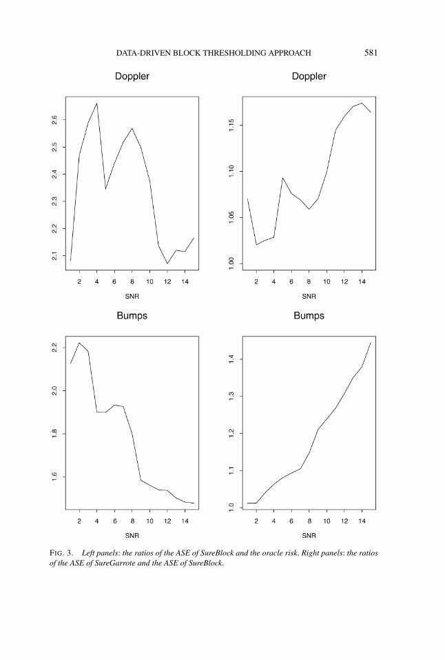
j,k ∧σ 2,where θj,k are the true wavelet coefficients. Furthermore, to examine the advantageof empirically selecting block sizes, we compare the ASE of SureBlock with that ofan estimator we call SureGarrote which empirically chooses the threshold at eachlevel but fixes the block size L = 1. Figure 3 summarizes the numerical resultsfor Doppler and Bumps with n = 1024, SNR ranging from 1 to 15 and 100 repli-cations. SureBlock consistently outperforms SureGarrote in all cases. The ASEof SureGarrote is up to 40 percent higher than the corresponding ASE of Sure-Block (see the right panels in Figure 3). Furthermore risk of SureBlock is withina small factor of the corresponding oracle risk. For Doppler the ratios of the ASEof SureBlock and the oracle risk are between 2 to 2.7 and for Bumps the ratiosare between 1.5 to 2.2 (see the left panels in Figure 3). In these simulations theblock sizes chosen by SureBlock vary from 1 to 16, depending on the resolutionlevels. This example shows that the SureBlock procedure works well relative to theideal oracle risk and empirically selecting block sizes improves the performancenoticeably relative to the SureGarrote procedure. It would be interesting to carryout a more extensive numerical study to compare the performance of SureBlockwith many other procedures including the empirical Bayes estimator of Johnstoneand Silverman (2005). We leave this to future work.

5. Theoretical properties of SureBlock. We now turn to the theoretical prop-erties of SureBlock for the nonparametric regression problem (1) under the inte-grated mean squared error R(f , f ) = E‖f − f ‖2

2. The asymptotic results showthat the SureBlock procedure is strongly adaptive.

Besov spaces are a very rich class of function spaces and contain as special casesmany traditional smoothness spaces such as Hölder and Sobolev spaces. Roughlyspeaking, the Besov space Bα

p,q contains functions having α bounded derivativesin Lp norm, the third parameter q gives a finer gradation of smoothness. Full de-tails of Besov spaces are given, for example, in Triebel (1983) and DeVore andLorentz (1993). For a given r-regular mother wavelet ψ with r > α and a fixedprimary resolution level j0, the Besov sequence norm ‖ · ‖bα

p,qof the wavelet coef-

ficients of a function f is then defined by

‖f ‖bαp,q

= ‖ξj0

‖p +( ∞∑

j=j0

(2js‖θj‖p)q

)1/q

,(18)

where ξj0

is the vector of the father wavelet coefficients at the primary res-olution level j0, θj is the vector of the wavelet coefficients at level j , and

s = α + 12 − 1

p> 0. Note that the Besov function norm of index (α,p, q) of

a function f is equivalent to the sequence norm (18) of the wavelet coeffi-cients of the function. See Meyer (1992). The Besov body Bα

p,q(M) is defined by


FIG. 3. Left panels: the ratios of the ASE of SureBlock and the oracle risk. Right panels: the ratiosof the ASE of SureGarrote and the ASE of SureBlock.


Bαp,q(M) = {f :‖f ‖bα

p,q≤ M}. The minimax risk of estimating f over the Besov

body Bαp,q(M) is

R∗(Bαp,q(M)) = inf

fsup

f ∈Bαp,q(M)

E‖f − f ‖22.(19)

Donoho and Johnstone (1998) show that the minimax risk R∗(Bαp,q(M)) converges

to 0 at the rate of n−2α/(1+2α) as n → ∞.The blockwise James–Stein estimation of the wavelet coefficients and the cor-

responding function f is determined by the block size Lj and threshold level λj

of each resolution j . Let L = (Lj )j≥j0 with 1 ≤ Lj ≤ 2j/2, and λ = (λj )j≥j0 withλj ≥ 0. Let fL,λ be the corresponding estimator of f . The minimax risk among allblock James–Stein estimators with all possible block sizes L and threshold levels λ

is

R∗T (Bα

p,q(M)) = inffL,λ

supf ∈Bα

p,q(M)

E‖fL,λ − f ‖22(20)

and equivalently

R∗T (Bα

p,q(M)) = infλj≥0,1≤Lj≤2j/2

supθ∈Bα

p,q (M)

E

∞∑j=j0

‖θ j (λj ,Lj ) − θj‖22.

We shall call R∗T (Bα

p,q(M)) the minimax block thresholding risk. It is clear thatR∗

T (Bαp,q(M)) ≥ R∗(Bα

p,q(M)). Theorems 4 and 5 below show R∗T (Bα

p,q(M)) iswithin a small constant factor of the minimax risk R∗(Bα

p,q(M)). The followingtheorem shows that SureBlock adaptively attains the exact minimax block thresh-olding risk R∗

T (Bαp,q(M)) asymptotically over a wide range of Besov bodies.

THEOREM 3. Suppose the mother wavelet ψ is r-regular. Let f ∗ be the Sure-Block estimator of f defined in (17). Then

supf ∈Bα

p,q(M)

Ef ‖f ∗ − f ‖22 ≤ R∗

T (Bαp,q(M))

(1 + o(1)

)(21)

for 1 ≤ p,q ≤ ∞, 0 < M < ∞, and r ≥ α > 4( 1p

− 12)+ + 1

2 with 2α2−1/61+2α

> 1/p.

Theorem 3 is proved in Section 6. The main technical tools for the proof are theoracle inequalities for SureBlock developed in Section 2.2.

Theorems 4 and 5 below make it clear that the SureBlock procedure is indeednearly optimally adaptive over a wide collection of Besov bodies Bα

p,q(M) includ-ing both the dense (p ≥ 2) and sparse (p < 2) cases. The estimator is asymp-totically sharp adaptive over Besov bodies with p = q = 2 in the sense that itadaptively attains both the optimal rate and optimal constant. Over Besov bodieswith p ≥ 2 and q ≥ 2 SureBlock adaptively achieves within a factor of 1.25 of


the minimax risk. At the same time the maximum risk of the estimator is simul-taneously within a constant factor of the minimax risk over a collection of Besovbodies Bα

p,q(M) in the sparse case of p < 2.

THEOREM 4. Suppose ψ is r-regular. (i) SureBlock is adaptively sharp mini-max over Besov bodies Bα

2,2(M) for all M > 0 and r ≥ α > 0.88, that is,

supf ∈Bα

2,2(M)

Ef ‖f ∗ − f ‖22 ≤ R∗(Bα

2,2(M))(1 + o(1)

).(22)

(ii) SureBlock is adaptively, asymptotically within a factor of 1.25 of the mini-max risk over Besov bodies Bα

p,q(M),

supf ∈Bα

p,q (M)

Ef ‖f ∗ − f ‖22 ≤ 1.25R∗(Bα

p,q(M))(1 + o(1)

)(23)

for all p ≥ 2, q ≥ 2, M > 0 and 2α2−1/61+2α

> 1/p with r ≥ α > 1/2.

For the sparse case p < 2, the SureBlock estimator is also simultaneously withina small constant factor of the minimax risk.

THEOREM 5. Suppose ψ is r-regular. SureBlock is asymptotically minimaxup to a constant factor G(p ∧ q) over a large range of Besov bodies with 1 ≤p,q ≤ ∞, 0 < M < ∞, and r ≥ α > 4( 1

p− 1

2)+ + 12 with 2α2−1/6

1+2α> 1/p. That is,

supf ∈Bα

p,q(M)

Ef ‖f ∗ − f ‖22 ≤ G(p ∧ q) · R∗(Bα

p,q(M))(1 + o(1)

),(24)

where G(p ∧ q) is a constant depending only on p ∧ q .

6. Proofs. Throughout this section, without loss of generality, we shall as-sume the noise level σ = 1. We first prove Theorem 1 and then use it as the maintool to prove Theorem 3. The proofs of Theorems 4 and 5 and Proposition 1 aregiven later.

6.1. Notation and preparatory results. Before proving the main theorems, weneed to introduce some notation and collect a few technical results. The proofs ofsome of these preparatory results are long. For reasons of space these proofs areomitted here. We refer interested readers to Cai and Zhou (2005) for the completeproofs.

Consider the normal mean problem (2) with σ = 1. For a given block size L

and threshold level λ, set rb(λ,L) = Eθb‖θ b(λ,L) − θb‖2 and define r(λ,L) =

1d

∑mb=1 rb(λ,L) = ED(λ,L), where D(λ,L) = 1

d

∑mb=1 ‖θ b(λ,L) − θb‖2

2. Set

R(θ) = infλ≤λF ,1≤L≤d1/2

r(λ,L) = infmax{L−2,0}≤λ≤λF ,1≤L≤d1/2

r(λ,L).(25)


The difference between R(θ) and Rblock.oracle(θ) defined in (10) is that thesearch range for the threshold λ in R(θ) is restricted to be at most λF . The re-sult given below shows that the effect of this restriction is negligible for any blocksize L.

LEMMA 1. For any fixed η > 0, there exists a constant Cη > 0 such that forall θ ∈ Rd ,

R(θ) − Rblock.oracle(θ) ≤ Cηdη−1/2.

The following lemma is adapted from Donoho and Johnstone (1995) and is usedin the proof of Theorem 1.

LEMMA 2. Let Td = d−1 ∑(x2

i − 1) and μd = d−1‖θ‖22. If γ 2

d d/ logd → ∞,then

supμd≥3γd

(1 + μd)P (Td ≤ γd) = o(d−1/2).

We also need the following bounds for the loss of the SureBlock estimator. Thisbound is used in the proof of Theorem 3.

LEMMA 3. Let {xi : i = 1, . . . , d} be given as in (2). Then

‖θ∗ − θ‖22 ≤ 4d logd + 2‖z‖2

2.(26)

Finally we develop a key technical result for the proof of Theorem 1. Set

U(λ,L) = 1

dSURE(x, λ,L)

= 1 + 1

d

m∑b=1

(λ2 − 2λ(L − 2)

S2b

I (S2b > λ) + (S2

b − 2L)I (S2b ≤ λ)

).

Note that both D(λ,L) and U(λ,L) have expectation r(λ,L).The goal is to show that the minimizer (λS,LS) of U(λ,L) is asymptot-

ically the ideal threshold level and block size. The key step is to show that d = |ED(λS,LS) − infλ,L r(λ,L)| is negligible for max{L − 2,0} ≤ λ ≤λF and 1 ≤ L ≤ d1/2. Note that for two functions g and h defined on thesame domain, | infx g(x) − infx h(x)| ≤ supx |g(x) − h(x)|. Hence, |U(λS,LS) −infλ,L r(λ,L)| = | infλ,L U(λ,L) − infλ,L r(λ,L)| ≤ supλ,L |U(λ,L) − r(λ,L)|and consequently

d ≤ E

∣∣∣∣D(λS,LS) − r(λS,LS) + r(λS,LS)

− U(λS,LS) + U(λS,LS) − infλ,L

r(λ,L)

∣∣∣∣(27)

≤ E supλ,L

|D(λ,L) − r(λ,L)| + 2E supλ,L

|r(λ,L) − U(λ,L)|.


The upper bounds for the two terms on the RHS of (27) is given as follows.

PROPOSITION 2. Let λF = 2L logd . Uniformly in θ ∈ Rd , we have

Eθ supmax{L−2,0}≤λ≤λF ,1≤L≤d1/2

|U(λ,L) − r(λ,L)| ≤ cd−1/4(logd)5/2,(28)

Eθ supmax{L−2,0}≤λ≤λF ,1≤L≤d1/2

|D(λ,L) − r(λ,L)| ≤ cd−1/4(logd)5/2.(29)

The following result, which is crucial for the proof of Theorem 5, plays the rolesimilar to that of Proposition 13 in Donoho and Johnstone (1994b).

PROPOSITION 3. Let X ∼ N(μ,1) and let Fp(η) denote the probability mea-sures F(dμ) satisfying

∫ |μ|pF (dμ) ≤ ηp . Let r(δgλ, η) = supFp(η){EF rg(μ) :∫ |μ|pF (dμ) ≤ ηp} where rg(μ) = Eμ(δ

gλ(x) − μ)2 and δ

gλ(x) = (1 − λ2

x2 )+x. Let

p ∈ (0,2) and λ = √2 logη−p, then r(δ

gλ, η) ≤ 2ηpλ2−p(1 + o(1)) as η → 0.

The following lemma bounds the approximation errors between the mean ofthe empirical wavelet coefficient and the true wavelet coefficient of f ∈ Bα

p,q(M).

Set β = α − 1/p, which is positive under the assumption 2α2−1/61+2α

> 1/p in Theo-rems 3, 4 and 5.

LEMMA 4. Let θ = (θj,k) be the DWT of the sampled function {n−1/2f ( kn)}

with n = 2J and let θj,k = ∫f (x)ψj,k(x) dx. Then ‖θ − θ‖2

2 ≤ Cn−2β .

REMARK 1. Lemma 4 implies

infλj≥0,1≤Lj≤2j/2

supθ∈Bα

p,q(M)

E

∞∑j=j0

‖θ j (λj ,Lj ) − θ j‖22

(30)= (

1 + o(1))R∗

T (Bαp,q(M))

and for p ≥ 2 and q > 2

supθ∈Bα

p,q(M)

∞∑j=j0

∑k

( θ2j,k/n

θ2j,k + 1/n

)(31)

= (1 + o(1)

)sup

θ∈Bαp,q(M)

∞∑j=j0

∑k

( θ2j,k/n

θ2j,k + 1/n

)


under the assumption 2α2−1/61+2α

> 1/p which implies β > α/(2α+1). The argumentfor (30) is as follows. Write

E

∞∑j=j0

‖θ j (λj ,Lj ) − θ j‖22 − E

∞∑j=j0

‖θ j (λj ,Lj ) − θj‖22

= ‖θ − θ‖22 + 2E

∞∑j=j0

〈θ j (λj ,Lj ) − θj , θj − θ j 〉.

From Lemma 4, ‖θ − θ‖22 ≤ Cn−2β = o(n−2α/(2α+1)). The Cauchy–Schwarz in-

equality implies

supθ∈Bα

p,q(M)

E

∞∑j=j0

〈θ j (λj ,Lj ) − θ j , θj − θ j 〉

= supθ∈Bα

p,q(M)

‖θ − θ‖2

√√√√E

∞∑j=j0

‖θ j (λj ,Lj ) − θj‖22,

which is o(n−2α/(2α+1)), since ‖θ − θ‖2 = O(n−β) with β > α/(2α + 1) andR∗

T (Bαp,q(M)) ≤ Cn−2α/(1+2α) logn from Cai (1991) in which Lj = logn and

λj = 4.505 logn. We know R∗T (Bα

p,q(M)) ≥ R∗(Bαp,q(M)) ≥ Cn−2α/(1+2α) from

Donoho and Johnstone (1998). Thus (30) is established. The argument for (31) issimilar.

In the following proofs we will denote by C a generic constant that may varyfrom place to place.

6.2. Proof of Theorem 1. The proof of Theorem 1 is similar to but more in-volved than those of Theorem 4 of Donoho and Johnstone (1995) and Theorem 2of Johnstone (1999) because of variable block size.

Set Td = d−1 ∑(x2

i − 1) and γd = d−1/2 log3/22 d . Define the event Ad = {Td ≤

γd} and decompose the risk of SureBlock into two parts:

R(θ∗, θ) = d−1Eθ {‖θ∗ − θ‖22I (Ad)} + d−1Eθ {‖θ∗ − θ‖2

2I (Acd)}

≡ R1,d(θ) + R2,d(θ).

We first consider R1,d(θ). On the event Ad , the signal is sparse and θ∗ is thenonnegative garrote estimator θ∗

i = (1 − 2 logd/x2i )+xi by the definition of θ∗

in (8). Decomposing R1,d(θ) further into two parts with either μd = d−1‖θ‖22 ≤

3γd or μd > 3γd yields that R1,d(θ) ≤ RF (θ)I (μd ≤ 3γd)+ r1,d(θ) where RF (θ)

is the risk of the nonnegative garrote estimator and r1,d(θ) = d−1Eθ {‖θ∗ −


θ‖22I (Ad)}I (μd > 3γd). The oracle inequality (3.10) in Cai (1991) with L = 1

and λ = λF = 2 logd yields that

RF (θ) ≤ d−1∑i

[(θ2i ∧ λF ) + 4(π logd)−1/2d−1]

(32)≤ d−1[‖θ‖2

2 + 4(π logd)−1/2].Recall that μd = ‖θ‖2

2/d and γd = d−1/2 log3/22 d . It then follows from (32) that

RF (θ)I (μd ≤ 3γd) ≤ d−1[3d1/2 log3/22 d + 4(π logd)−1/2](33)

≤ cd−1/4(logd)5/2.

Note that on the event Ad , ‖θ∗‖22 ≤ ‖x‖2

2 ≤ d + dγd and so

r1,d(θ) ≤ 2d−1(E‖θ∗‖22 + ‖θ‖2

2)P (Ad)I (μd > 3γd)

≤ 2(1 + 2μd)P (Ad)I (μd > 3γd) = o(d−1/2),

where the last step follows from Lemma 2. Note that for any η > 0, Lemma 1yields that

R(θ) − Rblock.oracle(θ) ≤ Cηdη−1/2(34)

for some constant Cη > 0 and for all θ ∈ Rd . Equations (27)–(29) yield

R2,d(θ) − R(θ) ≤ d ≤ cd−1/4(logd)5/2.(35)

The proof of part (a) of the theorem is completed by putting together (33)–(35).We now turn to part (b). It follows from part (a) that R(θ∗, θ) ≤ Rblock.oracle(θ)+

cd−1/4(logd)5/2. Note that Rblock.oracle(θ) ≤ r(d1/2 − 2, d1/2). Stein’s unbiasedrisk estimate and Jensen’s inequality yield that

r(d1/2 − 2, d1/2) = d−1∑b

(d1/2 − (d1/2 − 2)2E

1

‖Xb‖2

)

≤ d−1∑b

(d1/2 − (d1/2 − 2)2 1

E‖Xb‖2

).

Note that E‖Xb‖2 = ‖θb‖2 + d1/2. Hence r(d1/2 − 2, d1/2) ≤ d−1 ∑b(d

1/2 +1 − d

‖θb‖2+d1/2 ). The elementary inequality (∑m

i=1 ai)(∑m

i=1 a−1i ) ≥ m2, for ai >

0,1 ≤ i ≤ m yields that

Rblock.oracle(θ) ≤ r(d1/2 − 2, d1/2) ≤ d−1(d + d1/2 − d2

‖θ‖22 + d

)

= ‖θ‖22

‖θ‖22 + d

+ d−1/2


and part (b) then follows. We now consider part (c). Note first that R1,d(θ) ≤RF (θ). On the other hand, R2,d(θ) = d−1E{‖θ∗ − θ‖2

2I (Acd)} ≤ Cd−1(E‖θ∗ −

θ‖42)

1/2P 1/2(Acd). To complete the proof of (12), it then suffices to show that under

the assumption μd ≤ 13γd , E‖θ∗−θ‖4

2 is bounded by a polynomial of d and P(Acd)

decays faster than any polynomial of d−1. Note that in this case ‖θ‖22 = dμd ≤

d1/2 log3/22 d . Since ‖θ∗‖2

2 ≤ ‖x‖22 and xi = θi + zi ,

E‖θ∗ − θ‖42 ≤ E(2‖θ∗‖2

2 + 2‖θ‖22)

2

≤ E(2‖x‖22 + 2‖θ‖2

2)2 ≤ E(4‖θ‖2

2 + 2‖z‖22)

2

≤ 32‖θ‖42 + 8E‖z‖4

2 ≤ 32d log32 d + 16d + 8d2.

On the other hand, it follows from Hoeffding’s inequality and Mill’s inequality that

P(Acd) = P

(d−1

∑(z2

i + 2ziθi + θ2i − 1) > d−1/2 log3/2

2 d)

≤ P(d−1

∑(z2

i − 1) > 13d−1/2 log3/2

2 d)

+ P(d−1

∑2ziθi > 1

3d−1/2 log3/22 d

)≤ 2 exp(−C log3

2 d) + 12 exp(−C log3

2 d/μd),

which decays faster than any polynomial of d−1.

6.3. Proof of Theorem 2. Note that x/(x +d) is increasing in x and for p ≥ 2,supθ∈�p(τ) ‖θ‖2 = d1/2−1/pτ . Hence

supθ∈�p(τ)

R(θ∗, θ) ≤ supθ∈�p(τ)

‖θ‖22

‖θ‖22 + d

+ cd−1/4(logd)5/2

≤ supθ∈�p(τ) ‖θ‖22

supθ∈�p(τ) ‖θ‖22 + d

+ cd−1/4(logd)5/2

= d1−2/pτ 2

d1−2/pτ 2 + d+ cd−1/4(logd)5/2

= τ 2

τ 2 + d2/p+ cd−1/4(logd)5/2.

Now consider part (b). It follows from Proposition 3 that there is a constant cp

depending on p such that R(θ) ≤ infλ≥0 r(λ,1) ≤ cd−1τp(log(dτ−p))(2−p)/2,since �p(τ) = {θ ∈ R

d :‖θ‖pp/d ≤ τp/d}. Part (b) now follows directly from (11)

in Theorem 1.


For part (c) it is easy to check that for 0 < p ≤ 2, ‖θ‖22 ≤ ‖θ‖2

p ≤ τ 2 <

13d1/2 log3/2

2 d and so μd ≤ 13γd . It then follows from Theorem 1 and (39) that

R(θ∗, θ) ≤ RF (θ) + cd−1(logd)−1/2

≤ 1

d

(‖θ‖22 + 8(2 logd)−1/2) + cd−1(logd)−1/2

≤ 1

dτ 2 + cd−1(logd)−1/2.

6.4. Proof of Theorem 3. Again we set σ = 1. Note that the empirical waveletcoefficients yj,k can be written as yj,k = θj,k + n−1/2zj,k , where θj,k = Eyj,k

are the DWT of the sampled function {n−1/2f ( in)} and zj,k

i.i.d.∼ N(0,1). To moreconveniently use Theorem 1, we multiply both sides by n1/2 and get

y′j,k = θ ′

j,k + zj,k, j ≥ j0, k = 1,2, . . . ,2j ,(36)

where y′j,k = n1/2yj,k and θ ′

j,k = n1/2θj,k . Let f = ∑2J

k=1 n−1/2f ( in)φJ,k(t),

where n = 2J . Note that supf ∈Bαp,q(M) ‖f − f ‖2

2 = o(n−2α/(1+2α)) from Lemma 4.To establish Theorem 3, by the Cauchy–Schwarz inequality as in Remark 1, it suf-fices to show that

supf ∈Bα

p,q(M)

Ef ‖f ∗ − f ‖22 ≤ R∗

T (Bαp,q(M))

(1 + o(1)

).

Fix 0 < ε0 < 1/(1 + 2α) and let J0 be the largest integer satisfying 2J0 ≤ nε0 .Write

n−1Eθ ′‖θ ′∗ − θ ′‖22 =

( ∑j≤J0

∑k

+ ∑J0≤j<J1

∑k

+ ∑j≥J1

∑k

)n−1Eθ ′‖θ ′∗ − θ ′‖2

2

= S1 + S2 + S3,

where J1 > J0 is to be chosen later. The terms S1 and S3 are identical in all blockthresholding procedures. We thus only focus on the term S2. Since 0 < ε0 < 1/(1+2α), nε0n−1 logn = o(n−2α/(1+2α)). It then follows from (26) in Lemma 3 thatS1 ≤ Cnε0n−1 logn = o(n−(2α)/(1+2α)) which is negligible relative to the minimaxrisk. On the other hand, it follows from (11) in Theorem 1 that

S2 ≤ ∑J0≤j<J1

n−12jR(θ ′j ) + ∑

J0≤j<J1

n−12jRF (θ ′j )I (μ′

2j ≤ 3γ2j )

+ ∑J0≤j<J1

n−1c23j/4j5/2

= S21 + S22 + S23,

where μ′2j = 2−j‖θ ′

j‖22 = 2−jn‖θ j‖2

2 and γ2j = 2−j/2j3/2. It follows from Re-


mark 1 that

S21 = ∑J0≤j<J1

n−12jR(θ ′j ) ≤ (

1 + o(1))R∗

T (Bαp,q(M)).(37)

We shall see that both S22 and S23 are negligible relative to the minimax risk. Notethat

S23 = ∑J0≤j<J1

n−1c23j/4j5/2 ≤ Cn−123J1/4J5/21 .(38)

The oracle inequality (3.10) in Cai (1991) with L = 1 and λ = λF = 2 log(2j )

yields that

2jRF (θ ′j ) ≤

2j∑k=1

(nθj,k ∧ λF ) + 8(2 log 2j )−1/22−j

(39)≤ n‖θ j‖2

2 + 8(2 log 2j )−1/22−j .

Recall that μ′2j = 2−jn‖θ j‖2

2 and γ2j = 2−j/2j3/2. It then follows from (39) that

S22 = ∑J0≤j<J1

n−12jRF (θ ′j )I (μ′

2j ≤ 3γ2j )

(40)≤ ∑

J0≤j<J1

(3n−12j/2j3/2 + 8n−1(2 log 2j )−1/22−j ) ≤ Cn−12J1/2J

3/21 .

Hence if J1 satisfies 2J1 = nγ with some γ < 43(1+2α)

, then (38) and (40) yield

S22 + S23 = o(n−(2α)/(1+2α)).(41)

We now turn to the term S3. It is easy to check that for θ ∈ Bαp,q(M), ‖θj‖2

2 ≤M22−2α′j where α′ = α−( 1

p− 1

2)+ > 0. Note that if J1 satisfies 2J1 = nγ for some

γ > 11/2+2α′ , then for all sufficiently large n and all j ≥ J1, 2−jn‖θj‖2

2 ≤ 14γ2j

where γ2j = 2−j/2j3/2 which implies μ′2j ≤ 1

3γ2j for j ≥ J1 and γ > 2(1 − 2β),since

μ′2j − 2−jn‖θj‖2

2 ≤ 2−jn‖θ j − θj‖22 ≤ C2−jn1−2β = o(2−j/2j3/2).(42)

It thus follows from (12) and (39) that

S3 = ∑j≥J1

∑k

n−1Eθ ′(θ′∗j,k − θ ′

j,k)2

≤ ∑j≥J1

(n−12jRF (θ ′

j ) + cn−1j−j/2)≤ ∑

j≥J1

‖θ j‖22 + Cn−1(43)


≤ ∑j≥J1

‖θj‖22 + Cn−1 + ‖θ − θ‖2

2 ≤ C2−2α′J1 + Cn−1

= o(n−(2α)/(1+2α)),

when γ > α(1+2α)α′ and β > α

1+2α. Equations (41)–(43) hold by choosing γ satis-

fying

max{

α

(1 + 2α)α′ ,2(1 − 2(α − 1/p)

),

1

1/2 + 2α′}

< γ <4

(1 + 2α)3,

which is possible for α > 4( 1p

− 12)+ + 1

2 with 2α2−1/61+2α

> 1/p. This completes theproof.

6.5. Proof of Theorem 4. Define the minimax linear risk by

R∗L(Bα

p,q(M)) = infθ linear

supθ∈Bα

p,q (M)

E‖θ − θ‖22.

It follows from Donoho, Liu and MacGibbon (1990) and Remark 1 that

R∗L(Bα

p,q(M)) = (1 + o(1)

)sup

θ∈Bαp,q (M)

∞∑j=j0

∑k

( θ2j,k/n

θ2j,k + 1/n

),

R∗L(Bα

p,q(M)) = R∗(Bαp,q(M))(1 + o(1)) for p = q = 2, and R∗

L(Bαp,q(M)) ≤

1.25R∗(Bαp,q(M))(1 + o(1)) for all p ≥ 2 and q ≥ 2. It thus suffices to show that

SureBlock asymptotically attains the minimax linear risk for α > 0, p ≥ 2 andq ≥ 2. Since ‖θ − θ‖2

2 = o(n−2β) with β > α/(1 + 2α), we need only to showsupθ∈Bα

p,q(M) Eθ‖θ∗ − θ‖22 ≤ R∗

L(Bαp,q(M))(1 + o(1)) similar to the arguments in

Remark 1.Recall in the proof of Theorem 3 it is shown that Eθ‖θ∗ − θ‖2

2 ≤ S1 +S21 + S22 + S23 + S3, where S1 + S22 + S23 + S3 = o(n−2α/(2α+1)) and S21 =∑

J0≤j<J1n−12jR(θ ′

j ) with J0 and J1 chosen as in the proof of Theorem 3. Since

the minimax risk R∗(Bαp,q(M)) � n−2α/(2α+1), this implies that S21 is the domi-

nating term in the maximum risk of SureBlock. It follows from the definition ofR(θ ′

j ) given in (10) that n−12jR(θ ′j ) ≤ n−1 ∑

b Eθ ′b‖θ ′

b(Lj −2,Lj )−θ ′b‖2

2, wherethe RHS is the risk of the blockwise James–Stein estimator with any fixed blocksize 1 ≤ Lj ≤ 2j/2 and a fixed threshold level Lj − 2. Stein’s unbiased risk esti-

mate [see, e.g., Johnstone (2002), Chapter 9.2] yields that n−1 ∑b Eθ ′

b‖θ ′

b(Lj −2,Lj ) − θ ′

b‖22 ≤ ∑

b(‖θ b‖2

2Lj/n

‖θ b‖22+Lj/n

+ 2n). Hence the maximum risk of SureBlock sat-

isfies

supθ∈Bα

p,q (M)

Eθ‖θ∗ − θ‖22

≤ supθ∈Bα

p,q(M)

∑J0≤j<J1

∑b

( ‖θ b‖22Lj/n

‖θ b‖22 + Lj/n

+ 2

n

)· (

1 + o(1))


≤ supθ∈Bα

p,q(M)

∑J0≤j<J1

∑b

( ‖θb‖2Lj/n

‖θb‖2 + Lj/n+ 2

n

)· (

1 + o(1))

= supθ∈Bα

p,q(M)

( ∑J0≤j<J1

∑b

‖θb‖22Lj/n

‖θb‖22 + Lj/n

+ 2∑

J0≤j<J1

2j

nLj

)· (

1 + o(1)),

where the second inequality follows from a similar argument as in Remark 1. Notethat in the proof of Theorem 1, J1 satisfies 2J1 = nγ with γ < 4

(1+2α)3 . Hence

if Lj satisfies 2jρ ≤ Lj ≤ 2j/2 for some ρ > 14 , then

∑j≤J1

2j

nLj≤ 1

n2 · 2J13/4 =

o(n−(2α)/(1+2α)) and hence

supθ∈Bα

p,q(M)

Eθ‖θ∗ − θ‖22

(44)

≤ supθ∈Bα

p,q (M)

∑J0≤j<J1

∑b

( ‖θb‖2Lj/n

‖θb‖2 + Lj/n

)· (

1 + o(1)).

Note that∑2j /Lj

b=1‖θb‖2Lj/n

‖θb‖2+Lj/n= 2j

n− (

Lj

n)2 ∑2j /Lj

b=11

‖θb‖2+Lj/n. Then the simple

inequality (∑m

i=1 ai)(∑m

i=1 a−1i ) ≥ m2, for ai > 0,1 ≤ i ≤ m yields that

∑J0≤j<J1

∑b

( ‖θb‖2Lj/n

‖θb‖2 + Lj/n

)≤ 2j

n−

(Lj

n

)2(2j

Lj

)2 2j /Lj∑b=1

(‖θb‖2 + Lj

n

)

= 2j /n∑2j /Lj

b=1 ‖θb‖2∑2j /Lj

b=1 ‖θb‖2 + 2j /n

(45)

= 2j /n∑

k |θj,k|2∑k |θj,k|2 + 2j /n

.

Theorem 2 in Cai, Low and Zhao (2000) shows that

supθ∈Bα

p,q(M)

∑J0≤j<J1

2j /n∑

k |θj,k|2∑k |θj,k|2 + 2j /n

= R∗L(Bα

p,q(M))(1 + o(1)

).(46)

The proof is complete by combining (44)–(46).

6.6. Proof of Theorem 5. Set ρg(η) = infλ supFp(η) EF rg(μ) where Fp(η) and

rg(μ) are given as in Proposition 3. Proposition 3 implies that ρg(η) ≤ r(δgλ, η) ≤

2ηp(2 logη−p)(2−p)/2(1 + o(1)) as η → 0. For p ∈ (0,2), Theorem 15 of Donoho

and Johnstone (1994b) shows the univariate Bayes minimax risk satisfies ρ(η) =

infδ supFp(η) EF Eμ(δ(x) − μ)2 = ηp(2 logη−p)(2−p)/2(1 + o(1)) as η → 0. Notethat ρg(η)/ρ(η) is bounded as η → 0 and ρg(η)/ρ(η) → 1 as η → ∞. Both ρg(η)

and ρ(η) are continuous on (0,∞), so G(p) = supηρg(η)

ρ(η)< ∞, for p ∈ (0,2).


Theorems 4 and 5 in Section 4 of Donoho and Johnstone (1998) derived the as-ymptotic minimaxity over Besov bodies from the univariate Bayes minimax esti-mators. It then follows from an analogous argument of Section 5.3 in Donoho andJohnstone (1998) that

R∗T (Bα

p,q(M)) ≤ infλj

supθ∈Bα

p,q(M)

E

∞∑j=j0

‖θ j (λj ,1) − θj‖2

≤ G(p ∧ q) · R∗(Bαp,q(M))

(1 + o(1)

).

APPENDIX: TEST FUNCTIONS

FIG. A.1. Test functions.


REFERENCES

ANTONIADIS, A. and FAN, J. (2001). Regularization of wavelet approximations (with discussion).J. Amer. Statist. Assoc. 96 939–967. MR1946364

BREIMAN, L. (1995). Better subset regression using the nonnegative garrote. Technometrics 37373–384. MR1365720

CAI, T. (1999). Adaptive wavelet estimation: A block thresholding and oracle inequality approach.Ann. Statist. 27 898–924. MR1724035

CAI, T., LOW, M. G. and ZHAO, L. (2000). Blockwise thresholding methods for sharp adaptiveestimation. Technical report, Dept. Statistics, Univ. Pennsylvania.

CAI, T. and SILVERMAN, B. W. (2001). Incorporating information on neighboring coefficients intowavelet estimation. Sankhya Ser. B 63 127–148. MR1895786

CAI, T. and ZHOU, H. (2005). A data-driven block thresholding approach to wavelet estimation.Technical report, Dept. Statistics, Univ. Pennsylvania.

CHICKEN, E. (2005). Block-dependent thresholding in wavelet regression. J. Nonparametr. Statist.17 467–491. MR2130851

CHICKEN, E. and CAI, T. (2005). Block thresholding for density estimation: Local and global adap-tivity. J. Multivariate Anal. 95 76–106. MR2164124

DAUBECHIES, I. (1992). Ten Lectures on Wavelets. SIAM, Philadelphia, PA. MR1162107DEVORE, R. and LORENTZ, G. G. (1993). Constructive Approximation. Grundlehren der Math-

ematischen Wissenschaften [Fundamental Principles of Mathematical Sciences] 303. Springer,Berlin. MR1261635

DONOHO, D. L. and JOHNSTONE, I. M. (1994a). Ideal spatial adaptation by wavelet shrinkage.Biometrika 81 425–455. MR1311089

DONOHO, D. L. and JOHNSTONE, I. M. (1994b). Minimax risk over lp-balls for lq -error. Probab.Theory Related Fields 99 277–303. MR1278886

DONOHO, D. L. and JOHNSTONE, I. M. (1995). Adapt to unknown smoothness via wavelet shrink-age. J. Amer. Statist. Assoc. 90 1200–1224. MR1379464

DONOHO, D. L. and JOHNSTONE, I. M. (1998). Minimax estimation via wavelet shrinkage. Ann.Statist. 26 879–921. MR1635414

DONOHO, D. L., LIU, R. C. and MACGIBBON, B. (1990). Minimax risk over hyperrectangles, andimplications. Ann. Statist. 18 1416–1437. MR1062717

EFROMOVICH, S. Y. (1985). Nonparametric estimation of a density of unknown smoothness. Theor.Probab. Appl. 30 557–661. MR0805304

GAO, H.-Y. (1998). Wavelet shrinkage denoising using the nonnegative garrote. J. Comput. Graph.Statist. 7 469–488. MR1665666

HALL, P., KERKYACHARIAN, G. and PICARD, D. (1998). Block threshold rules for curve estima-tion using kernel and wavelet methods. Ann. Statist. 26 922–942. MR1635418

HALL, P., KERKYACHARIAN, G. and PICARD, D. (1999). On the minimax optimality of blockthresholded wavelet estimators. Statist. Sinica 9 33–50. MR1678880

JOHNSTONE, I. M. (1999). Wavelet shrinkage for correlated data and inverse problems: Adaptivityresults. Statist. Sinica 9 51–84. MR1678881

JOHNSTONE, I. M. (2002). Function estimation and Gaussian sequence model. Unpublished manu-script.

JOHNSTONE, I. M. and SILVERMAN, B. W. (2005). Empirical Bayes selection of wavelet thresh-olds. Ann. Statist. 33 1700–1752. MR2166560

KERKYACHARIAN, G., PICARD, D. and TRIBOULEY, K. (1996). Lp adaptive density estimation.Bernoulli 2 229–247. MR1416864

MEYER, Y. (1992). Wavelets and Operators. Cambridge Studies in Advanced Mathematics 37. Cam-bridge Univ. Press, Cambridge. Translated from the 1990 French original by D. H. Salinger.MR1228209

http://www.ams.org/mathscinet-getitem?mr=1946364






















STEIN, C. (1981). Estimation of the mean of a multivariate normal distribution. Ann. Statist. 91135–1151. MR0630098

STRANG, G. (1992). Wavelet and dilation equations: A brief introduction. SIAM Rev. 31 614–627.MR1025484

TRIEBEL, H. (1983). Theory of Function Spaces. Monographs in Math. 78. Birkhäuser, Basel.MR0781540

DEPARTMENT OF STATISTICS

THE WHARTON SCHOOL

UNIVERSITY OF PENNSYLVANIA

PHILADELPHIA, PENNSYLVANIA 19104USAE-MAIL: [email protected]

DEPARTMENT OF STATISTICS

YALE UNIVERSITY

NEW HAVEN, CONNECTICUT 06511USAE-MAIL: [email protected]




mailto:[email protected]

mailto:[email protected]

a data-driven block thresholding approach to …hz68/sureblock.pdfa data-driven block thresholding...

Documents