A Decomposition Algorithm for Local AccessTelecommunications Network Expansion

Planning

Anantaram Balakrishnan,Thomas L. Magnanti

andRichard T. Wong

WP# 3496-92-MSA September, 1992

A Decomposition Algorithm forLocal Access Telecommunications Network

Expansion Planning

Anantaram Balakrishnan*§Thomas L. Magnanti §

Sloan School of ManagementM. I. T.

Cambridge, MA

Richard T. Wong

AT&T Bell LaboratoriesHolmdel, NJ

Revised: September 1992

t This research was initiated through a grant from GTE Laboratories Incorporated, Waltham,

Massachusetts

Supported in part by a research award from the AT&T Foundation§ Supported in part by a NATO Collaborative research grant CRG 900281

Abstract

Growing demand, increasing diversity of services, and advances in transmission andswitching technologies are prompting telecommunication companies to rapidlyexpand and modernize their networks. This paper develops and tests adecomposition methodology to generate cost-effective expansion plans, withperformance guarantees, for one major component of the network hierarchy-thelocal access network connecting customers to the local switching center. The modelcaptures economies of scale in facility costs, and addresses the central tradeoffbetween installing concentrators and expanding cables to accommodate demandgrowth. By exploiting the special tree and routing structure of the expansionplanning problem, our solution method integrates two major algorithmic strategiesfrom mathematical programming-the use of valid inequalities, obtained bystudying a problem's polyhedral structure, and dynamic programming, which can beused to solve an uncapacitated version of the local access network expansionplanning problem. The computational results for three actual test networksdemonstrate that this enhanced dynamic programming algorithm, when embeddedin a Lagrangian relaxation scheme (with problem preprocessing and localimprovement), is very effective in generating good upper and lower bounds:implemented on a personal computer, the method was able to generate solutionsthat are within 1.2 to 7.0% of optimality. In addition to developing a successfulsolution methodology for a practical problem, this paper illustrates the possibility ofeffectively combining decomposition methods and polyhedral approaches.

Keywords: Integer programming decomposition, concentrator location,telecommunications planning, polyhedral methods

1. Introduction

Advances in switching and transmission technologies combined with growingdemand, increasing diversity of services, and deregulation of thetelecommunications industry have prompted telephone companies to rapidlyupgrade and expand their networks. Modernization of the local access networks,which connect switching centers to customers, is a particularly important prioritysince these networks account for over 50% of the total investment incommunication facilities (according to Standard and Poor's Industry Surveys [1992],the total value of plant in 1990 exceeded 250 billion dollars in the U. S. alone); yetthey are not as technologically advanced as the higher levels-the long-distance andinter-office networks-in the telecommunications network hierarchy. For instance,over 80% of the local access networks still use analog transmission over coppercables. However, recent technology and cost trends in the industry have improvedthe economic and technical viability of introducing electronic switching and fiberoptic transmission to increase capacity in local access networks.

The new technologies such as electronic remote units (or multiplexers) introducediscrete choice decisions and spatial couplings between different parts of thenetwork, thus vastly increasing the number of possible ways to meet growingdemand. Traditional manual planning methods that consider only the option ofadding more cables to expand capacity are no longer adequate. Sincetelecommunication investments are so expensive (total annual investments by U. S.local exchange companies is approximately $20 billion, Telephony [1991]), a costeffective network expansion plan can offer considerable economic value. Forinstance, Jack, Kai, and Shulman [1992] report savings of over $30 million per year atGTE using an interactive decision support system to assist network planners.

This paper develops and tests an optimization-based methodology to identify aminimum cost network expansion plan to meet increasing demand. We formulatean integer programming model, validated by consulting network planners inindustry, that captures the essential tradeoffs between concentrator location and cableexpansion, and accommodates economies of scale in investment and operating costs.Although the model approximates the expansion costs as piecewise-linear concavefunctions, and does not consider investment timing decisions, it is an importantbuilding block for detailed, multi-period planning systems (see, for example,Shulman and Vachani [19901). To solve the local access network expansion model,we develop a decomposition method combining Lagrangian relaxation with adynamic programming algorithm that exploits the problem's special tree structureand routing restrictions. Since the basic problem formulation does not providesatisfactory lower bounds, we identify several classes of valid inequalities thatstrengthen the model's linear programming relaxation. Unlike other cutting planemethods that use general purpose linear programming codes to solve the enhanced

-1-

formulations (e.g., Hoffman and Padberg [1985]), we modify the dynamicprogramming algorithm to directly incorporate the valid inequalities. Ourcomputational tests using representative data (obtained from industry) demonstratethat the method generates good upper and lower bounds. Thus, this paper not onlydevelops an effective solution method for the important practical problem of localaccess network design, but also adds to the growing literature demonstrating theusefulness of polyhedral methods for solving difficult, large-scale optimizationproblems.

The rest of this paper is organized as follows: Section 2 presents a formaldefinition of the local access network planning problem, reviews our modelingassumptions, and describes a basic mixed-integer programming formulation.Section 3 describes an efficient dynamic programming algorithm to solve theuncapacitated version of the local access network planning problem, develops aLagrangian relaxation scheme that uses the dynamic program to solve anuncapacitated subproblem, and outlines a Lagrangian-based heuristic procedure. InSection 4 we describe two algorithmic enhancements-a problem preprocessingprocedure to eliminate variables, and a coefficient reduction method to strengthenthe problem formulation. Section 5 presents three classes of valid inequalities, andshows how to modify the dynamic program to incorporate them. Section 6 describesour implementation, and presents computational results for three networksprovided to us by a major telephone company. We illustrate how the validinequalities dramatically improve the lower bounds (by about 80%) relative to thebasic model, and we study the robustness of the method to changes in demand andcost parameters. Our results show that the combination of Lagrangian relaxation,dynamic programming, and polyhedral methods permits us, using a personalcomputer, to efficiently find solutions that are within 1.2 to 7.0% of optimality.Section 7 identifies directions for further work.

2. The Basic Local Access Network Expansion Model

2.1 Problem descriptionThe local access network (also called the feeder loop, central office network,

outside plant, or customer access network) connects customer nodes (control ordistribution points, in telecommunication parlance) to the switching center (alsocalled the central office). Each customer node is a collection point for individualcustomers (possibly hundreds) connected via a subsidiary distribution network.Balakrishnan et al. [19911 and Jack et al. [1992] describe the technologies andcharacteristics of local access networks in greater detail. Most current local accessnetworks have a tree structure, rooted at the switching center (Shulman andVachani [19901). Edges of the tree correspond to physical sections of underground oroverhead cables.

-2-

III

All communications to and from each customer node flow through the assignedswitching center. Each node has a demand, measured by the required number ofcircuits from that node to the switching center. In conventional copper networks,each circuit requires a dedicated twisted copper pair which we will call a cable. Anode's demand depends on the number and type (e.g., residential or commercial) ofindividual customers connected to it. The local access network can satisfy thisdemand in two ways: either provide a dedicated cable (from the customer node tothe switching center) for each required circuit, or route the circuits through a trafficcompression device called a concentrator. Concentrators are electronic devices thatcombine incoming signals (e.g., analog signals) on several lines into a singlecomposite signal (e.g., high frequency digital or optical signal) that requires only oneoutgoing line. In practice, a variety of devices such as electronic multiplexers,remote switches, and fiber optic terminals can perform traffic compression (seeBalakrishnan et al. [1991]). We collectively refer to all these different technologies asconcentrators. Our planning model distinguishes between different technologiesthrough their installation and operating cost functions.

As customer demand increases (for example, due to new construction, customermovement, or new services), the existing cables and concentrators can no longeraccommodate the required number of circuits from each node. In the expansionplanning problem, we wish to locate new concentrators, selectively expand cablecapacities, and reroute traffic from customer nodes via concentrators in order tosatisfy the projected demand using the minimum possible total network expansioncost. By routing traffic through concentrators, we reduce the downstream (or centraloffice side) cable requirements. This tradeoff between installing concentrators andexpanding cable capacities is central to the local access network expansion problem.We next introduce some notation and formally describe the expansion planningmodel and its assumptions.

Notation and problem parametersLet T denote the given (undirected) rooted tree over which the local access

network expansion problem is defined. The nodes of this network representcustomer nodes and/or potential concentrator locations, and its edges correspond tocable sections. We index the set of nodes N from 0 to n, with the root node 0representing the switching center. Let d i denote the projected demand at eachcustomer node i. The capacity Bij of edge (i,j) is the number of existing cables in the

section connecting nodes i and j. For simplicity, all our subsequent discussionsassume that the existing network does not contain any concentrators; however, ourmethod extends easily to problems with existing concentrators.

Let Pij denote the (unique) path in the tree connecting nodes i and j. To provide

one circuit from node i to the switching center, we must reserve one cable on eachedge of the path Pi0. Since the existing network does not have adequate capacity to

-3-

meet the projected demand, one or more edges of the current network must haveprojected exhaust, i.e., the number of available cables on that edge is less than thetotal demand for all nodes communicating through that edge to the switchingcenter.

Cost structureOur model minimizes the total cost of installing concentrators and adding cables

to meet the projected demand. The model and solution methodology can alsoincorporate additional node-to-concentrator connection costs (e.g., to disconnect thecurrent circuit and reroute it through a concentrator at a different location) which weignore for simplicity. Cable expansion costs vary by edge (depending on the lengthand location of the cable section), and has both a fixed and variable component. Oneach edge (i,j), we incur a fixed cable cost Gij (e.g., to install additional ducts or poles)and a variable cable cost eij that might represent, for instance, investment in cables ormaintenance expenses. Concentrator costs also have location-dependent fixed andvariable components. The fixed concentrator cost Fj models land acquisition andinfrastructure investments at node j, while the variable concentrator cost cj reflects

the purchase price and operating expenses of concentrator modules. As we notelater, the concentrator cost also includes the cost of the required high-speedconcentrator-to-switching center connection.

Our solution procedure also applies when concentrator and cable expansion costshave the more general piecewise-linear, concave structure shown in Figure 1; eachsegment in this function might correspond, for instance, to a different concentratortechnology or transmission medium. The true cost of concentrators (or cableexpansion) is a step function of the required capacity since concentrator modules areavailable only in discrete units; however, our analysis of actual cost estimates andinformation provided by our industrial collaborator suggest that a piecewise-linear,concave function can adequately approximate this cost especially for long-termplanning purposes (due to rapid technological changes, predicting the costs exactlyfor, say, a 5-year time horizon is often very difficult). Although we haveimplemented and tested the solution method for problems with concaveconcentrator costs, for expositional ease in describing the model formulation andsolution algorithm, we will assume the simpler fixed plus variable cost structure forboth cable expansion and concentrator location. (We do, however, indicate how theapproach will handle concave costs.)

2.2 Modeling assumptionsTo reduce the complexity of managing and maintaining the local access network,

planners often impose several restrictions on the permissible expansion options androuting patterns. Discussions with planners in industry suggest that the followingfour modeling assumptions reflect or adequately approximate current practice.

-4-

III

Shulman and Vachani [1990] and Jack et al. [1992] use similar assumptions in theirsuccessful decision support system for local access network planning.

Assumption Al: Single-level concentrationTraffic originating at any node of the network is concentrated at most once beforereaching the switching center.

Assumption A2: Non-bifurcated routingA single concentrator (or the switching center) processes the entire demand of eachcustomer node.

Assumption A3: Contiguity restrictionEvery concentrator serves a contiguous region surrounding it, i.e., if a concentratorat node j serves node i, then this concentrator also serves all other nodes (includingnode j) on the connecting path Pij.

Assumption A4: Transmission cost for concentrated trafficConcentrated traffic (flowing from each concentrator to the switching center) eitherconsumes a negligible amount of existing cable capacity, or uses a dedicated umbilicalconnection (also called a remote-to-host connection) whose cost depends only on thelocation and throughput of the concentrator. In the latter case, we can incorporatethe cost of the umbilical connection in the concentrator cost.

Assumption Al reflects current state-of-the-art in local access network design.Introducing multiple levels of concentration within the local access network is oftenuneconomical given the current costs of cables and concentrators. Assumptions A2and A3 reflect operational convenience. For example, maintaining and repairingnetworks with multiple routes from each customer node or non-contiguousconcentrator service regions can be burdensome. Assumption A4 greatly simplifiesthe model and improves solution effectiveness, while introducing only minordistortions in total cost or actual capacity usage. For instance, one digital copper pair,also called a T1 span, can accommodate up to 96 voice channels (see, for example,Jack et al. [1992]); thus a customer node that previously required, say, 1000 copperpairs for analog transmission, requires only 11 T1 spans to transmit compressedsignals from that node. If the "concentrator" includes a fiber optic terminal, the fibercable connecting the terminal to the switching center might replace an existingcopper cable.

Since the local access network has a tree structure, assumptions Al and A2together imply that assigning a concentrator (or switching center) to each node icompletely specifies the routing decisions in the network. We say that node i homeson node j if a concentrator located at node j processes node i's traffic. In this case, thetraffic from node i is routed on d i cables along the unique path Pij to node j, where it

-5-

is concentrated and transmitted via the remote-to-host connection from node j tothe switching center. Any node whose traffic is not concentrated is said to home onthe switching center; equivalently, we assume that the switching center always has aconcentrator. We permit backfeed or flow away from the switching center, i.e., aconcentrator at node j can also serve downstream nodes that are closer than node j tothe switching center. The contiguity assumption (A3) reduces the concentratorselection and assignment problem to one of decomposing (and covering) the treeinto subtrees, and selecting one concentrator location within each subtree to serve itstraffic requirements. We use this observation to efficiently solve an uncapacitatedsubproblem using dynamic programming.

To illustrate these concepts, consider the local access network shown in Figure 2.The dashed edges in this network are sections with projected exhaust. For instance,the current capacity of 1675 units on edge (26, 34) is less than the total demand (2203units) of nodes 34 and 41. Hence, we must either expand this edge by 528 units inorder to home nodes 34 and 41 on a downstream concentrator (or the switchingcenter), or install a concentrator at either of these nodes. For instance, a concentratorat node 34 can serve both nodes 34 and 41. Since we permit backfeed, we can alsohome the downstream nodes, say nodes 26, 18, and 12, on this concentrator. Noticethat, if we use this homing strategy, we need not expand edges (26, 34), (18, 26), and(12, 18) since their existing capacities can accommodate the required backflow. Also,if node 7 homes on the concentrator at node 34, the contiguity property specifies thatnode 13 (and node 19) cannot home on the switching center; this node must eitherhome on node 34 or on a concentrator located at nodes 13 or 19.

2.3 Basic Integer Programming FormulationIn the local network expansion planning problem we consider, we are given the

projected demand at each customer node, the existing cable capacity in each section,and the costs for adding cables and installing concentrators at each location. Weneed to decide:

* where to locate concentrators, and with what capacity;* which edges (cable sections) to expand, and by how much;* how to route the traffic from each node to the switching center; and,* in a more general model, which concentrator technology to use at each

node.

Our formulation uses the following decision variables:

Assignment xij = 1 if node i homes on node j,variable 0 otherwise;

Concentrator yj = 1 if we install a concentrator at node j,location variable 0 otherwise;

-6-

III

Cable Zi (Zji) = 1 if we expand cable capacity from node i toinstallation variable node j (node j to node i),

0 otherwise; and,

Cable ij (sj) = number of cables added from node i to node j

expansion variable (j to i).

We use directed variables to model cable installation and expansion, i.e., althoughedges are undirected, we distinguish between expansion in the i-to-j direction andthe j-to-i direction on each edge (i,j). Using directed cable addition variablesincreases the formulation size but strengthens the model's linear programmingrelaxation, thus improving our algorithm's performance. To emphasize thedirection of flow, we will consider two directed arcs, denoted as <i,j> and <j,i>,corresponding to each original undirected edge (i,j); both arcs have the same fixedand variable cable expansion costs as the original edge. We also redefine Pij as thedirected path from node i to node j in the tree. We assume, for convenience, thateach customer node can home on any other node in the network. In practice, wemight prohibit certain node-to-concentrator assignments (e.g., due to proximityrestrictions limiting the maximum distance a concentrator can serve in order toensure good transmission quality), in which case we can eliminate thecorresponding assignment variables.

The Local Access Network Expansion Planning Problem has the following basicmixed-integer programming formulation:

Network Expansion Planning Model [LAN1]

minimize , Fjyj + Z Z (dicj)xij + Gijzi + eijsij (21)jE N ie N je N <i,j> T <i,j> T

subject to

Assignment constraints:I xij = 1 all i N, (2.2)jeN

Concentrator location constraints:y = xj allje N, (2.3)

Contiguity restrictions:

xij xk i all i,j E N, (2.4)

-7-

Cable capacity constraints:

I d k xkl <k,leODij

Bij + Sij + Sji all (i,j) T,

Cable installation-forcing constraints:

Sij < Mij Zij

Arc orientation constraints:

zij + Zji 1

Integrality/Nonnegativity constraints:

j Xij, Zig Zji = orisij sji 2 0

all <i,j> T,

all (i,j) E T, and

all j N, (i,j)e T, and

all (i,j) e T.

In this formulation,ki. is the node adjacent to node i on path Pij,Obij is the set of all node pairs k,l whose connecting path Pkl contains

edge (i,j), andMij (Mji) is an upper bound on the maximum required cable expansion on

edge (i,j) in the i-to-j (j-to-i) direction.

The objective function (2.1) minimizes the sum of the fixed and variableconcentrator costs, and the cable installation and expansion costs. Constraints (2.2)ensure that each node i is assigned to exactly one concentrator (possibly at theswitching center, in which case xi0 = 1). Equation (2.3) specifies that node i contains aconcentrator (yj = 1) if and only if this node homes on itself (i.e., xjj = 1). Constraints(2.4) models the contiguity restriction, i.e., if node i homes on node j, then node i'simmediate neighbor kij on the connecting path Pij must also home on j. The left-

hand side of the cable capacity constraint (2.5) expresses the total flow on edge (i,j) interms of the node-to-concentrator assignments that use this edge; we must add cablesif this flow exceeds the available capacity Bij. If we add cables on arc <i,j> (i.e., if s >0), constraint (2.6) forces the cable installation variable zij to assume a value of 1, thusabsorbing the fixed cable expansion cost Gij in the objective function. Constraint (2.7)

permits cable expansion on edge (i,j) in either the i-to-j or the j-to-i direction, but notboth.

The parameter Mij in the right-hand side of the forcing constraint (2.6a), which

we call the cable expansion bound, represents the maximum number of additionalcables that any optimal solution can possibly install on arc <i,j>. For instance, if Dij isthe total demand for all nodes k whose path Pkj contains arc <i,j>, we can set Mij =Max {0, Di0 - Bij } In Section 4.2, we show how to strengthen the formulation byusing tighter values for Mij.

-8-

(2.5)

(2.6)

(2.7)

(2.8)

(2.9)

III

Let us briefly indicate how we might incorporate piecewise-linear, concave costfunctions (Figure 1) instead of the simple fixed plus linear cost structure. Supposethe concentrator cost function consists of M linear segments (corresponding to Mdifferent concentrator types or technologies), with increasing fixed costs Fjm anddecreasing variable costs cjm as a function of the technology type m = 1,2,...M. Tocapture these costs, we replace yj and xii with disaggregate concentrator location andassignment variables Yjm and xijm for each segment m = 1,2,...,M. The binary variable

Yjm is 1 if the solution installs a type m concentrator at node j, and is 0 otherwise;similarly, xijm equals 1 if a type m concentrator at node j serves node i, and is 0

otherwise. We modify constraints (2.2) to (2.5) accordingly. Because the costfunction is concave, we need not introduce explicit concentrator capacity constraintssince the cost minimizing solution will automatically select the appropriatetechnology to process the required throughput at each concentrator location. We cansimilarly model piecewise-linear, concave cable expansion costs using disaggregatecable installation and expansion variables.

3. Decomposition Algorithm for the Basic Local Access NetworkPlanning Model

Formulation [LANI] is a large-scale mixed-integer program whose size increasesquadratically with the number of nodes. Like many other network design problems,this problem is NP-complete (Balakrishnan et al. [1992]). However, the uncapacitatedversion of this problem without existing cable cable capacities is easy to solve using apolynomial-time dynamic programming algorithm. We, therefore, propose aLagrangian relaxation approach that solves an uncapacitated subproblem to generategood upper and lower bounds. Our solution method consists of three components:(i) preprocessing and coefficient reduction, i.e., performing some prior analysis toreduce the problem size and strengthen the formulation; (ii) solving the Lagrangiansubproblems to generate lower bounds on the optimal cost; and (iii) generating goodheuristic solutions from the Lagrangian subproblem solutions. This section firstdiscusses the dynamic programming method for solving the uncapacitated problem,and develops the Lagrangian-based lower bounding and heursitic procedures. Insubsequent sections, we describe the preprocessing and coefficient reductionmethods, and propose various additional formulation and algorithmicenhancements to improve the method's performance.

3.1 Solving the Uncapacitated Local Access Network Planning ProblemGiven a tree network without existing cable capacities, and fixed and variable

costs for installing concentrators and cables, the uncapacitated local access networkplanning (ULAN) problem seeks the concentrator locations, homing patterns, andcable expansion plan that meets projected demand at minimum total cost. To

-9-

distinguish the cost parameters for the uncapacitated problem from the originalvalues, we let j and yj denote the fixed and variable concentrator costs at node j, and

let rij and Eij denote the fixed and variable cable costs on arc <i,j>. Later we willindicate how, using Lagrange multipliers, we compute the values of these"uncapacitated" cable and concentrator cost parameters from the original costs.

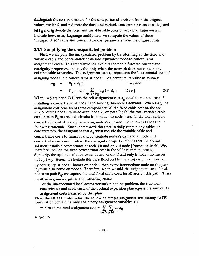
3.1.1 Simplifying the uncapacitated problemFirst, we simplify the uncapacitated problem by transforming all the fixed and

variable cable and concentrator costs into equivalent node-to-concentratorassignment costs. This transformation exploits the non-bifurcated routing andcontiguity properties, and is valid only when the network does not contain anyexisting cable capacities. The assignment cost aij represents the "incremental" cost of

assigning node i to a concentrator at node j. We compute its value as follows:

aij = 4) + d i f i = j, and

= rikij +d{ I CklI+di if i j. (3.1)1J <k,l>E Pij

When i = j, equation (3.1) sets the self-assignment cost ajj equal to the total cost of

installing a concentrator at node j and serving this node's demand. When i j, theassignment cost consists of three components: (a) the fixed cable cost on the arc<i,kij> joining node i to its adjacent node kij on path Pij; (b) the total variable cablecost on path Pij to create d i circuits from node i to node j; and (c) the total variable

concentrator cost at node j for serving node i's demand. Equation (3.1) has thefollowing rationale. Since the network does not initially contain any cables orconcentrators, the assignment cost aij must include the variable cable and

concentrator costs to transmit and concentrate node i's demand at node j. Ifconcentrator costs are positive, the contiguity property implies that the optimalsolution installs a concentrator at node j if and only if node j homes on itself. We,therefore, include the fixed concentrator cost in the self-assignment cost ajj.Similarly, the optimal solution expands arc <i,kij> if and only if node i homes onnode j, i * j. Hence, we include this arc's fixed cost in the i-to-j assignment cost aij.

By contiguity, if node i homes on node j, then every intermediate node on the pathPi must also home on node j. Therefore, when we add the assignment costs for allnodes on path Pi, we capture the total fixed cable costs for all arcs on this path. These

intuitive arguments justify the following claim:For the uncapacitated local access network planning problem, the true totalconcentrator and cable costs of the optimal expansion plan equals the sum of theassignment costs incurred by that plan.

Thus, the ULAN problem has the following simple assignment tree packing (ATP)formulation containing only the binary assignment variables xij:

minimize the total assignment cost = I aij xijieNjeN

subject to

-10-

II

assignment constraints (2.2), contiguity constraints (2.4), and xijE {0,1 } for all i,je N.

3.1.2 Dynamic Programming AlgorithmWe can solve the ATP formulation using Barany, Edmonds, and Wolsey's [19861

O(n2) dynamic programming algorithm. This algorithm is related to Kariv andHakimi's [1979] algorithm for solving the p-median problem on a tree. Barany et al.[1986] have also shown that the linear programming relaxation of the ATPformulation has integer extreme points.

To describe the dynamic program, let us introduce some notation andconventions. The level of a node i is the number of edges lying on path Pi0o Thus,

the root node (node 0) has level 0, its immediate successors have level 1, and so on.For convenience, we index the nodes in increasing order of their levels. For anynode i (i • 0) in the tree, let Pi denote its predecessor, and Si the set of all its

immediate successors. Let T(i) denote the subtree rooted at node i formed when wedelete edge (i,pi) from tree T.

Starting at the bottom of the tree, the dynamic programming procedurerecursively calculates, for each node i, the optimal total assignment cost TC(i) ofserving all nodes in subtree T(i) using only homing nodes (concentrators) locatedwithin this subtree. This tree cost TC(i) represents the optimal total networkexpansion cost if T(i) is a stand-alone tree. Hence, TC(O) is the optimal cost of theULAN problem.

To calculate TC(i), we must first determine where node i should home within itssubtree T(i). For any node j E T (note that j might lie outside T(i)), let HC(i,j) (HCstands for homing cost) denote the total cost of covering all nodes in subtree T(i),assuming node i homes on node i. Then,

TC(i) = minimum HC(i,j). (3.2)jE T(i)

The homing cost HC(i,j) consists of the i-to-j assignment cost aij plus the homing

costs of the subtrees rooted at node i's successors. By contiguity, if node i homes onnode j, then each successor u E Si must either home on node j, or home within its

subtree T(u). Therefore, the following recursive equations permit us to computeHC(i,j) for intermediate nodes i:

HC(i,j) = aij + ~ min(HC(u,j), TC(u)} if j=i or j T(i), and (3.3a)uSi

HC(ij) = aij + HC(v,j)+ min{HC(u,j), TC(u)} if j Tv), E S. (3.3b)UESI\ 1

-11 -

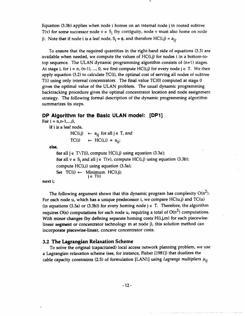
Equation (3.3b) applies when node i homes on an internal node j in rooted subtreeT(v) for some successor node v E Si (by contiguity, node v must also home on node

j). Note that if node i is a leaf node, Si = , and therefore HC(i,j) = aij.

To ensure that the required quantities in the right-hand side of equations (3.3) areavailable when needed, we compute the values of HC(i,j) for nodes i in a bottom-to-top sequence. The ULAN dynamic programming algorithm consists of (n+1) stages.At stage i, for i = n, (n-1), ..., 0, we first compute HC(i,j) for every node j e T. We then

apply equation (3.2) to calculate TC(i), the optimal cost of serving all nodes of subtreeT(i) using only internal concentrators. The final value TC(O) computed at stage 0gives the optimal value of the ULAN problem. The usual dynamic programmingbacktracking procedure gives the optimal concentrator location and node assignmentstrategy. The following formal description of the dynamic programming algorithmsummarizes its steps.

DP Algorithm for the Basic ULAN model: [DP1]For i = n,n-l,...,0,

if i is a leaf node,HC(i,j) v aij for all j E T, and

TC(i) - HC(i,i) = aii;

else,for all j E T\T(i), compute HC(i,j) using equation (3.3a);for all v E Si and all j E T(v), compute HC(i,j) using equation (3.3b);

compute HC(i,i) using equation (3.3a);Set TC(i) - Minimum HC(i,j);

j E T(i)next i;

The following argument shows that this dynamic program has complexity O(n2).For each node u, which has a unique predecessor i, we compare HC(u,j) and TC(u)

(in equations (3.3a) or (3.3b)) for every homing node j E T. Therefore, the algorithm

requires O(n) computations for each node u, requiring a total of O(n2 ) computations.With minor changes (by defining separate homing costs H(i,j,m) for each piecewise-linear segment or concentrator technology m at node j), this solution method canincorporate piecewise-linear, concave concentrator costs.

3.2 The Lagrangian Relaxation SchemeTo solve the original (capacitated) local access network planning problem, we use

a Lagrangian relaxation scheme (see, for instance, Fisher [1981]) that dualizes thecable capacity constraints (2.5) of formulation [LANI] using Lagrange multipliers uij

-12-

III

for all edges (i,j) e T (for directed arcs <i,j>, gij = gji by convention). The resulting

Lagrangian problem is:

minimize C di {c j + I kl xij + Fjyj + G ijzijiE N jN <k,l>e Pij jEN <i,j>E T

+ (eij gij) sij - gij Bij (3.4)<i,j>E T (i,j)e T

subject to constraints (2.2) - (2.4) and (2.6) - (2.9).

This problem decomposes into two subproblems: an ULAN subproblem, and a cableexpansion subproblem.

321 The ULAN subproblemThe uncapacitated network expansion subproblem, which we denote as

ULAN1 (), contains the x and y variables. Using our notation of Section 3.1.1, theULAN1 (g) subproblem has the following equivalent "uncapacitated" costparameters: 4j = Fj, yj = cj, Fri = 0, and kdw = Akl. Notice that this subproblem does notcontain fixed cable costs; our later formulation enhancements will strengthen theLagrangian relaxation by introducing arc fixed costs in the uncapacitated subproblem.For any given set of Lagrange multipliers {pk}, solving subproblem ULAN1 (g) usingour dynamic program gives a set of concentrator locations, and node-to-concentratorassignments that satisfy the contiguity and non-bifurcated routing properties. Welater use this subproblem solution to construct a feasible heuristic solution to theoriginal problem.

3.2.2 The Cable Expansion SubproblemThe cable expansion subproblem, denoted [CES(g)], determines the optimal

values of the cable installation and expansion variables, zij and sij, for all arcs <i,j>:

[CES(g)]minimize G Gij zi + I (eij - ij)ij (3.5)

<i,j>E T <i,j>E Tsubject to

sij < Mij ij all <i,j> e T, (3.6)

Zij+ zji 1 all (i,j) e T, and (3.7)

zij = or 1, si > O all <i,j> e T. (3.8)

This subproblem decomposes by edge, and is easy to solve. For each arc <i,j>, we firstexpress the optimal value of sij in terms of zij as follows:

sij = 0 if (eij - pij) > 0, and (3.9a)

-13-

sij = Mij Zij if (eij- ij) < 0. (3.9b)Substituting for sij in (3.5) gives the following cost coefficients for zij:

Gij(A) Gij + Mij min eij - gij, 0. (3.10)If Gij(g) and Gji(g) are both nonnegative, we set zij = zji = 0. Otherwise, we set ij = 1and zji = 0 if Gij(g) < Gji(g), and zij = 0 and zji = 1 if Gji(g) < Gij(g). Again, thissolution procedure extends easily to problems with piecewise-linear, concaveconcentrator costs.

For any nonnegative Lagrange multiplier vector g, the sum of the optimal valuesof the ULAN and cable expansion subproblems minus the term A, 9ij Bij gives a

(i,e Tlower bound on the optimal cost of [LAN1]. We use subgradient optimization (see,for instance, Held, Wolfe, and Crowder [19741 or Fisher [1981]) to heuristically adjustthe Lagrange multipliers to maximize the Lagrangian lower bound. Since the linearprogramming relaxations for both of our Lagrangian subproblems have integeroptimal solutions (Aghezzaf and Wolsey [19901 have shown this property for theULAN problem with piecewise-linear, concave costs), the best possible Lagrangianlower bound cannot exceed the optimal value of the linear programming relaxationof formulation [LAN1]. We next describe a method to obtain upper bounds on theoptimal value.

3.3 Lagrangian-based heuristic procedure

Our Lagrangian-based heuristic procedure first constructs a feasible startingsolution using the optimal values of subproblem ULANI(gi), and then applies a localimprovement procedure to further reduce the cost of this starting solution. Weconstruct the starting solution by "completing" the contiguous, non-bifurcated node-to-concentrator assignments chosen by subproblem ULAN1 (g), i.e., we compute theactual cable expansion required to accommodate the node-to-concentrator flows, andcompute the total concentrator and cable cost of this expansion plan. We then applya myopic improvement strategy called the Greedy Reassignment Heuristic thatiteratively reassigns nodes to concentrators, one at a time, without violating thecontiguity condition. To preserve contiguity, we need to only consider reassigningevery node i to each of the (I Si I +1) homing nodes of its neighbors. At each iteration,the greedy heuristic: (i) evaluates the cost impact of all feasible changes in node-to-concentrator assignments; and, (ii) performs the reassignment that gives the greatestreduction in total cost. If all feasible reassignments increase total cost, the localimprovement procedure terminates.

To reduce computational time, instead of improving the Lagrangian-basedstarting solution after every subgradient iteration, our implementation applies thegreedy method only intermittently (e.g., when the current Lagrangian starting

-14-

solution has lower cost than the previous best starting solution). We also use thegreedy heuristic to generate an initial upper bound, before performing thesubgradient procedure. We consider two different starting solutions for initialimprovement-a centralized solution that homes all demand nodes on the rootnode (i.e., this solution employs only cable expansion to satisfy projected demand),and a distributed solution that locates a concentrator at each node. The better of thetwo improved solutions provides the initial upper bound.

4. Modeling and Algorithmic Enhancements I: Variable Eliminationand Coefficient Reduction

Our preliminary computational experience (summarized in Section 6.2) with theLagrangian relaxation algorithm for the basic model [LAN1] suggested that, while theheuristic method generates very good solutions, the Lagrangian lower bounds areweak. To improve the lower bounds, we developed various modeling andalgorithmic enhancements. This section describes two types of improvements:problem preprocessing to eliminate certain assignment variables, and reducing thevalues of the cable expansion bounds Mij in order to tighten the forcing constraints

(2.6) in formulation [LAN1]. Section 5 describes new inequalities that furtherstrengthen the Lagrangian relaxation.

4.1 Variable Elimination by Problem PreprocessingTo reduce the size of problem [LAN1], we perform a tradeoff analysis to identify

suboptimal node-to-concentrator assignments a priori. Eliminating thecorresponding assignment variables xij from the problem formulation not only

reduces the problem size and computational effort, but might also improve thelower and upper bounds.

For each node pair i,j, our preprocessing method determines if node i can homeon node j in an optimal expansion plan by comparing a lower bound LJ on theincremental cost of assigning node i to node j to an upper bound Uii on the cost oflocating a concentrator at node i (and homing node i on this concentrator). If Lij >Uii, the i-to-j assignment is provably suboptimal, and we can eliminate theassignment variable xij from formulation [LAN1].

The lower bound Lij on the incremental cost of assigning node i to node j consists

of two components: an incremental cable expansion cost, and an incrementalconcentrator cost. To calculate the incremental cable expansion cost, consider any arc<k,l> on the path Pij connecting node i to node j. By contiguity, if node i homes onnode j, the total demand, say, Dik of all nodes on the path Pik (nodes i and k

inclusive) must flow through arc <k,l>. Let kl = Max { [Dik-Bkl], 01 denote the excess

-15-

flow on arc <k,l>. Node i contributes Min{~kl, d i} to this excess flow. Hence, Skl =

ekl Min(Okl, di} represents the incremental cable cost if node i homes on node j(note that we do not include the fixed cable cost Gkl in this incremental cost).

Adding the incremental costs 6kl for all arcs <k,/> of path Pij gives the cableexpansion cost component of the lower bound Lij. For the incremental concentratorcost, we use the variable concentrator cost cj d i incurred at node j to serve node i'sdemand. Thus, the lower bound Lij is:

Lij = I Sk + cjdi for all i,j E N. (4.1)<k,l>e T P..

If node i is a leaf node of T, and if the current capacity of the incident arc (i,kij) is lessthan node i's demand, we can improve the lower bound Lij by adding the fixed costGikij to the right-hand side of (4.1).

The upper bound Uii on the incremental cost when node i homes on itself is the

total concentrator cost to process node i's demand, i.e.,Uii = Fi + ci di for all i N. (4.2)

If Lij > Uii, the i-to-j assignment is provably suboptimal. For, suppose an optimal

expansion plan assigns node i to a concentrator at node j. Let N(i,j) be the subset ofnodes (including node i) that currently home on node j via node i. For every nodek E N(i,j), canceling the k-to-j assignment saves at least Lij/d i per unit demand,

while reassigning node k to a new concentrator at node i incurs a cost of at mostUii/d i per unit demand (due to concavity of concentrator costs). Therefore, if Lij >Uii, we can improve the current solution by installing a new concentrator at node i,and reassigning all nodes in N(i,j) to this concentrator (all the nodes on path Pij

except node i continue to home on the concentrator at node j), contradicting theoptimality of the given solution.

This preprocessing technique extends easily to piecewise-linear, concave costfunctions (to compute Lij we use the lowest variable cable cost eklm on each arc <k,l>

E Pij, and the lowest variable concentrator cost cjm at node j among all available

technologies m). The preprocessing method not only reduces the number ofvariables and constraints in the integer programming formulation but alsostrengthens it by decreasing the maximum possible flows (and hence the cableexpansion bounds Mij) on certain arcs.

4.2 Tightening the Cable Forcing Constraints by Coefficient ReductionTo improve the relaxation lower bounds of formulation [LAN1], we first tighten

the cable installation forcing constraints (2.6) by reducing the cable expansion boundsMij. Recall that Mij represents the largest possible value of the cable expansionvariable sij in any optimal solution. In Section 2.3, we computed Mij as the

-16-

III

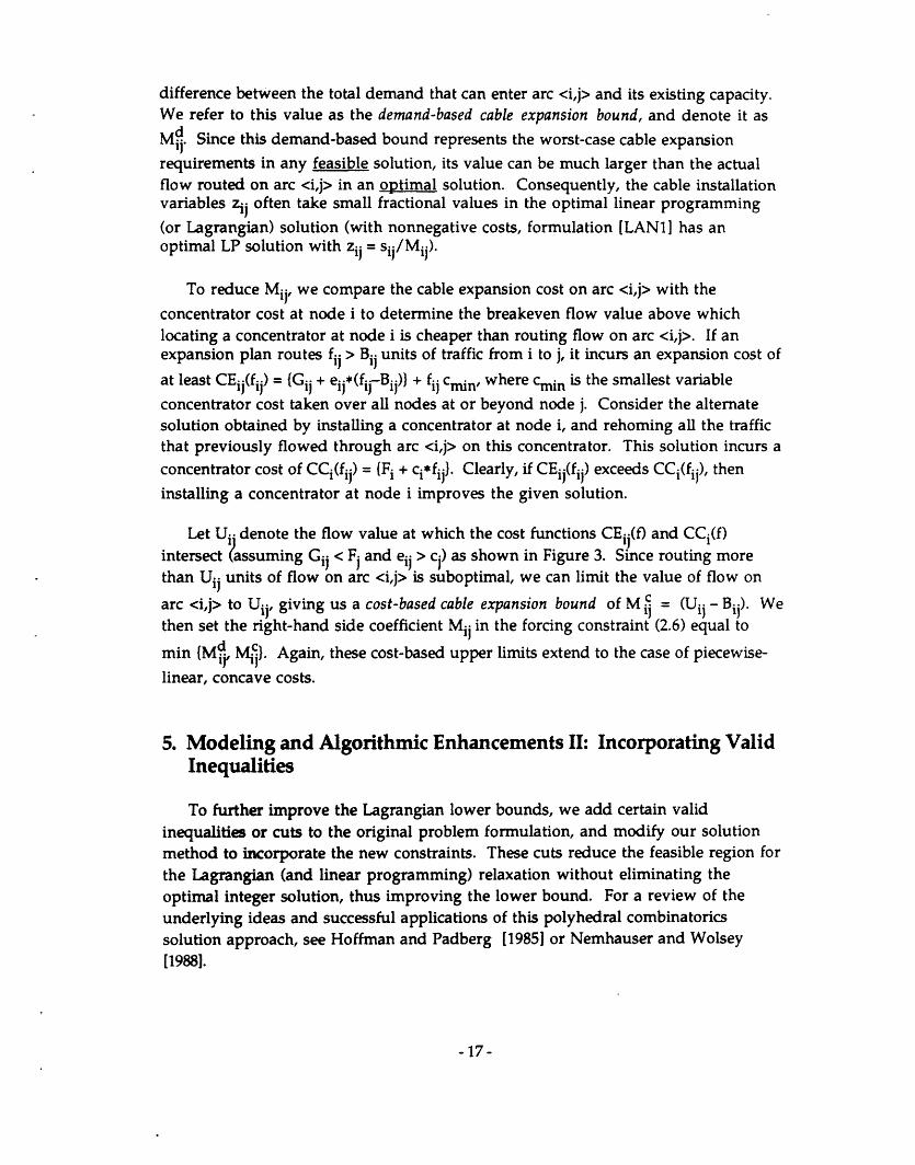
difference between the total demand that can enter arc <i,j> and its existing capacity.We refer to this value as the demand-based cable expansion bound, and denote it as

Md . Since this demand-based bound represents the worst-case cable expansionrequirements in any feasible solution, its value can be much larger than the actualflow routed on arc <i,j> in an optimal solution. Consequently, the cable installationvariables zij often take small fractional values in the optimal linear programming

(or Lagrangian) solution (with nonnegative costs, formulation [LAN1] has anoptimal LP solution with zij = sij/Mij).

To reduce Mij, we compare the cable expansion cost on arc <i,j> with the

concentrator cost at node i to determine the breakeven flow value above whichlocating a concentrator at node i is cheaper than routing flow on arc <i,j>. If anexpansion plan routes fij > Bij units of traffic from i to j, it incurs an expansion cost of

at least CEij(fij) = Gij + eij*(fij-Bij) + fij Cmin, where cmin is the smallest variableconcentrator cost taken over all nodes at or beyond node j. Consider the alternatesolution obtained by installing a concentrator at node i, and rehoming all the trafficthat previously flowed through arc <i,j> on this concentrator. This solution incurs aconcentrator cost of CCi(fij) = {Fi + ci*f ij)}. Clearly, if CEij(fij) exceeds CCi(fij), then

installing a concentrator at node i improves the given solution.

Let Ui. denote the flow value at which the cost functions CE.j(f) and CCi(f)intersect assuming Gij < F and ei > cj) as shown in Figure 3. Since routing morethan Uij units of flow on arc <i,j> is suboptimal, we can limit the value of flow on

arc <i,j> to Uij, giving us a cost-based cable expansion bound of M = (Uij - Bij). Wethen set the right-hand side coefficient Mij in the forcing constraint (2.6) equal to

min {Md Mi)}. Again, these cost-based upper limits extend to the case of piecewise-

linear, concave costs.

5. Modeling and Algorithmic Enhancements II: Incorporating ValidInequalities

To further improve the Lagrangian lower bounds, we add certain validinequalities or cuts to the original problem formulation, and modify our solutionmethod to incorporate the new constraints. These cuts reduce the feasible region forthe Lagrangian (and linear programming) relaxation without eliminating theoptimal integer solution, thus improving the lower bound. For a review of theunderlying ideas and successful applications of this polyhedral combinatoricssolution approach, see Hoffman and Padberg [19851 or Nemhauser and Wolsey[19881.

-17-

Balakrishnan et al. [1992] have identified several classes of valid inequalities forthe local access network expansion problem, and showed that, under certainconditions, these inequalities are facets of the integer programming polytope. In thispaper, we focus on a subset of those valid inequalities that are easy to incorporate inour dynamic programming algorithm for the Lagrangian subproblem. Theseconstraints relate the assignment variables xij and the cable installation andexpansion variables (zij and sij); adding them to the problem formulation results in a

single, comprehensive Lagrangian subproblem (instead of our previous twosubproblems) that simultaneously determines homing assignments, concentratorlocations, and cable additions.

Sections 5.1 to 5.3 motivate and describe the three classes of valid inequalities thatwe implemented. Section 5.4 describes requisite modifications to the dynamicprogramming method needed to accommodate these three types of inequalities. Ourcomputational experience indicates that these inequalities are very effective inreducing the gap between the Lagrangian lower and upper bounds.

Throughout this discussion, recall that T(i) is the subtree rooted at node i. Let D i

denote the total demand of all nodes in T(i); Pi is the predecessor of node i, and Si is

the set of node i's immediate successors.

5.1 Assignment-forcing Arc Installation InequalitiesOur first class of valid inequalities exploits the contiguity property to relate the

assignment variables xij to the binary cable installation variables zij. Assuming

positive arc expansion costs, any optimal local network expansion plan expands arc<i,k> only if node i homes on some node j via arc <i,k>. This observation motivatesthe following assignment-forcing arc installation inequalities:

E Xij > Zik for all arcs <i,k>. (5.1)j: <i,k>e Pij

Balakrishnan et al. [1992] generalize these constraints to cutsets of the tree T otherthan a single arc <i,k>.

5.2 Bottleneck-Arc Installation and Expansion InequalitiesOur next class of inequalities relate the concentrator location decisions to the

cable installation and expansion decisions. We refer to arc <i,Pi> as a bottleneck arcand node i as a bottleneck node if the total demand Di in subtree T(i) exceeds thearc's current capacity Bipi. Let IB denote the set of bottleneck nodes in T. For every

bottleneck node i IB, any feasible expansion plan must either install at least oneconcentrator within subtree T(i) or expand arc <i,pi> (or both). Furthermore, if

subtree T(i) does not contain any concentrators, the amount of capacity expansion onarc <i,pi> must be at least (Di - Bipi). Hence, we can add the following valid

bottleneck-arc installation and expansion inequalities to the problem formulation:

-18-

11

, Yk + zipi Ž 1 for all i E IB, and (5.2)ke T(i)

ke Yki) + s~, Ž for allie IB . (5.3)(Di-BiPi){ Z Yk + sipi > D i - Bip i foralli I (5-3)ke T(i)

Note that, if arc <i,pi> is not a bottleneck arc, then M P = 0 and we can eliminate thearc installation and expansion variables ipi and Sip i from the problem formulation.

Balakrishnan et al. [1992] generalize constraints (5.2) to subtrees of T other than therooted subtrees T(i) for i = 1,2,..., n.

5.3 Subtree-splitting Arc Installation and Expansion InequalitiesGiven any feasible expansion plan, we say that subtree T(i) completely homes on

an external node j T(i) if all nodes of T(i) home on node j in that expansion plan.On the other hand, T(i) partially homes on node j o T(i) if node j serves only a subsetof nodes in T(i) (including node i), and T(i) contains one or more concentrators thatserve the remaining nodes in this subtree. If all nodes in T(i) home onconcentrator(s) within T(i), we say that subtree T(i) is self-sufficient.

The bottleneck inequalities (5.2) and (5.3) apply when subtree T(i) completelyhomes on an external node j, in which case the total flow on arc <i,Pi> exactly equalsthe total demand subtree Di. On the other hand, when T(i) is self-sufficient, arc<i,pi> does not carry any flow; the assignment-forcing arc installation inequalities(5.1) prevent expanding arc <i,pi> in this case. We now consider additional valid

inequalities for situations when subtree T(i) partially homes on a node j e T(i). Forthe partial homing case, we do not know the exact flow on arc <i,pi>, but we can

compute upper and lower bounds on this flow. These bounds will vary dependingon the homing patterns in the "successor" subtrees, i.e., the subtrees rooted at nodei's successors. If, for a particular homing pattern, the upper bound (lower bound) isless (more) than arc <i,pi>'s capacity Bip i, then any solution containing that homing

pattern must not (must) expand arc <i,pi>. We will refer to this class of inequalitiesas Subtree-splitting Arc Installation and Expansion Inequalities since they exploit thedynamic program's strategy of splitting each subtree into its constituent successorsubtrees.

Let dminh denote the smallest leaf node demand in subtree T(h). If T(i) partiallyhomes on an external node j, then at least one leaf node in T(i) must home on aninternal concentrator (by contiguity); hence, the maximum possible flow on arc<i,pi> is (D i - dmini). Since node i homes outside T(i), the minimum flow on thisarc is d i. We might use these two bounds to decide if arc <i,pi> must necessarily beincluded (if d i > Bip i) or excluded (if Di-dmini < Bipi) when subtree T(i) partially

homes on any external node. We can further sharpen the upper and lower boundson arc <i,pi>'s flow by separately considering different combinations of homing

-19-

patterns in the successor subtrees. In general, every successor subtree can: (i)completely home on node j, (ii) partially home on node j, or (iii) be self-sufficient.However, since subtree T(i) partially homes on node j, at least one of its successorsubtrees must have a concentrator, i.e., we do not permit every successor subtree to

completely home on node j. Thus, we consider (3 1 Si I - 1) different successorhoming combinations. Each combination or case is characterized by a partition Q ={Sli, S2i, S3i} of the successor node set Si: Sl i, S2 i, and S3i correspond, respectively,

to the subsets of node i's successors whose rooted subtrees completely home on nodej, partially home on node j, or are self-sufficient in the chosen combination. Eachcase Q has associated upper and lower bounds on flow along arc <i,pi>; we next show

how to compute these bounds.

Calculating upper and lower bounds on flow on arc ,pi>:

Consider any successor node u E Si, and suppose u E Sl i for a given case Q i.e.,

T(u) completely homes on external node j. Then, the flow out of subtree T(u) exactly

equals the total demand D u in that subtree. If u E S3 i, then subtree T(u) is self-

sufficient, and no flow emanates from T(u). Finally, if T(u) partially homes on an

external node j (i.e., u E T2i) then, as we noted earlier ,the flow out of subtree T(u)cannot exceed (D u - dminu ) units but must be at least d u units.

Using these minimum and maximum outflows from the successor subtrees, wecan compute upper and lower bounds on arc <i,pi>'s flow as follows:

fmaxi (Q) = di+ I D + {Du-dminu , and (5.4)iPi i ue Sli uE S2i

fminipi(Q) = di + Du + S d u . (55)ue Sli ue S2i

If fminipi(Q) is greater than arc <i,pi>'s capacity Bip i, then we can add a valid

inequality specifying that arc <i,pi> must be IN, i.e., zip i = 1 and sipi (fminip i(Q)-

Bipi), whenever the solution selects the homing pattern Q. Similarly, if fmaxipi(Q) is

less than Bipi, we force arc <i,pi> to be OUT, i.e., zpi = spi = 0, for homing pattern Q.

Finally, if fminipi(Q) < Bip i < fmaxipi(Q), then arc <i,pi> is FREE, i.e., we permit Zip i

to be either 0 or 1, but ipi < (fmaxipi(Qi)-Bipi). We can formulate these logical

restrictions as mathematical constraints in terms of the assignment, concentratorlocation, and cable addition variables. For instance, to force arc <i,Pi> to be IN for acase Q (when fminipi(Q) > Bipi), we can add the following subtree-splitting arc

installation inequality:

Y, E x + C uk + 1ipi > (5.6)ue Sli le T(u) ke T(i) uE S2i ke T(i)

- 20 -

1I1

The first two terms in the left-hand side of (5.6) are both zero if the solution selects ahoming pattern consistent with case Q i.e., all nodes in subtrees T(u) for u E S1i and

all successors u E S2i home on a node outside T(i), in which case constraint (5.7)forces cable installation on arc <i,pi>. (We can tighten this subtree-splittingconstraint by including in the first term only assignment variables xlk corresponding

to leaf nodes I in subtrees T(u) for u E Sli; by contiguity, all nodes of subtree T(u)

must home on the external node j if all its leaf nodes home on node j.) The subtree-splitting constraint strengthens the original problem formulation, thus potentiallyimproving the Lagrangian (and LP) lower bounds. Similarly, we can formulate asubtree-splitting arc expansion constraint to enforce cable expansion ipi of at least

(fminipi(Q)-Bipi ) units for all IN arcs <i,pi> under case Q. We can also model the

OUT and FREE restrictions on arc <i,pi>. Since our dynamic programming approach

can implicitly account for these inequalities, we do not require explicit mathematicalrepresentations such as (5.6).

To summarize, for every node i, we consider each of the (31 Si I -1) casescorresponding to partial homing of subtree T(i). For every case Q we compute theupper and lower bounds on flow on arc <i,pi> using equations (5.4) and (5.5). By

comparing these bounds with the arc's capacity, we determine if we can restrict arc<i,pi> to be IN, OUT or FREE for homing pattern Q. In Section 5.4 we indicate how

to incorporate this information in the dynamic program. Note that the subtree-splitting arc installation inequality (5.6) generalizes our previous bottleneck-arcinstallation inequality (5.2). Recall that the bottleneck inequalities apply when thesubtree T(i) completely homes on an external node j. In this case, every successor ofnode i must also completely home on node j, i.e., the complete homing patterncorresponds to a case Q with S1i = Si, and S2i = S3i = 0. Applying equations (5.4) and(5.5) to this case, we find fmaxipi(Q) = fminipi(Q) = Di; hence, if D i > Bip i, i.e., if arc

<i,pi> is a bottleneck arc, then we must force arc <i,pi> to be IN whenever thesolution completely homes subtree T(i) on an external node j. Since S2i and S3i are

empty for this special case, the subtree-splitting arc installation inequality (5.6)reduces to the bottleneck-arc installation inequality (5.2). Similarly, the subtree-splitting arc expansion inequality (which imposes a lower bound on the arcexpansion variable sipi) generalizes the bottleneck-arc expansion inequality (5.3).

Our discussions thus far have focused on the case when node i homes on anexternal node j. Suppose T(i) is self-sufficient, i.e., node i homes on an internalconcentrator at node j E T(v) for some successor v e Si. In this case, we wish to use

the demand parameters to fix or restrict, if possible, the cable installation andexpansion variables for arc <i,v>. Since i homes on j E T(v), the successor subtreeT(v) must also be self-sufficient, but every other successor subtree T(u), for all u ESi\{v} can either completely home on j, partially home or j, or be self-sufficient.

-21 -

Thus, we can separately consider 31 Si I -1 combinations of successor homing patterns.Using our previous notation, we consider only cases Q with v S i. As before, wecan compute upper and lower bounds on the flow on arc <i,v> for each case. Thelower bound fminiv(Q) has the same form as equation (5.5). However, for the upperbound fmaxiv(Q) we must add to the right-hand side of equation (5.4) the totaldemand of all nodes outside subtree T(i). Again, we use these bounds to determineif arc <i,v> must be IN, OUT, or FREE for case Q, and impose the corresponding arcinstallation and expansion inequalities.

Our subtree-splitting inequalities consider combinations of homing patterns forthe immediate successors of node i. We can further refine this partition of homingpatterns and obtain sharper flow bounds (and, hence, tighter inequalities) byenumerating the homing patterns for subtrees that are two levels, three levels, andso on below node i. However, incorporating these inequalities in the dynamicprogram adds to the algorithmic complexity of the solution approach. Ourimplementation performs quite well with only the first level subtree-splittinginequalities.

5.4 Modifying the Dynamic Programming AlgorithmAdding the three classes of inequalities-the assignment-forcing, bottleneck-arc,

and subtree-splitting inequalities-to the original formulation introduces additionallinkages between the assignment, concentrator location, and cable addition variables.Consequently, when we dualize the cable capacity constraints (2.5) using multipliers

{ij}, the resulting Lagrangian subproblem, which we denote as [ULAN2(pg)],combines the previous uncapacitated network expansion problem [ULAN1(g)] andthe cable expansion subproblem [CES(g)]. This section describes how to modify theULAN dynamic programming approach [DP1] of Section 3.1 to solve the new,integrated Lagrangian subproblem.

To incorporate the new valid inequalities, we exploit the dynamic program'sability to account for (uncapacitated) arc fixed costs rij. These fixed costs were zero in

the uncapacitated subproblem ULAN1(g) for the basic formulation [LAN1. Addingthe inequalities of Sections 5.1 to 5.3 effectively introduces nonzero arc fixed coststhat vary depending on the homing pattern. Since our cost transformation(equation (3.1)) includes the arc fixed cost rik in the assignment cost aij only if k E Pij,we automatically satisfy the assignment-forcing cable installation inequalities (5.1),i.e., the Lagrangian subproblem solution does not install arc <i,k> if node i does nothome via node k.

We now show how the bottleneck-arc inequalities and the subtree-splittingconstraints determine the value of the arc fixed costs lik. Suppose, for some feasible

-22-

iI

case Q the subtree-splitting inequality for arc <i,k> specifies that this arc must be IN(since fminik(Qi) > Bik), i.e., Zik must be set to 1, and sik must be greater than orequal to (fminik(Q)-Bik) if the solution selects the homing pattern Q. Constraint

A

(2.6) together with the upper bound fmaxik(Q) specify an upper limit of Mik =min {Mik, fmaxik(Q)-Bik) on sik. The variables Zik and ik have coefficients of Gikand (eik-Pik) in the objective function of subproblem ULAN2(g); when arc <i,k> isforced to be IN, this subproblem has the following optimal solution:

Zik = 1, and

Sik = fminik(Q)-Bik if (eik-gik) > 0, andA

= Mik if (eik-gik) < 0.

Effectively, these optimal values contribute an equivalent "uncapacitated" arc fixedcost of

rik (Q) = Gik + min { (eik-gik) [fminik(Qi)-Bik], (eikj-4ik) Mik }. (5.7a)

Similarly, if the upper and lower bounds force arc <i,k> to be OUT or FREE (i.e., iffmaxik(Q) < Bik or fminik(Q) < Bik < fmaxik(Q)), we have the following equivalentfixed costs corresponding to homing pattern Q:

OUTrik(Q) - 0; or (5.7b)

FREE Ar ik (Q) - min (0, Gik + (eik- 9gik) Mik} (5.7c)

To recapitulate, for every feasible case Q we: (i) compute the upper and lowerbounds fmaxik(Q) and fminik(Q) for arc <i,k>, (ii) compare these bounds with theexisting capacity Bik to determine if arc <i,k> must be IN, OUT, or FREE, and (iii)

accordingly set the uncapacitated fixed cost rik(Q) for arc <i,k> corresponding case Q

equal to either rFk (Q), i(Q)Q), o r i k (Q). Since these arc fixed costs vary by case,applying our cost transformation (3.1) gives different assignment costs aij(Q) for

different homing patterns Q within subtree T(i). Consequently, the dynamicprogram must have the ability to differentiate the homing costs for various cases.

Recall that the dynamic program already treats the self-sufficient case separately;the tree cost TC(i) denotes the optimal total (assignment) cost of covering all nodesin rooted subtree T(i) assuming T(i) is self-sufficient. To distinguish betweencomplete and partial homing of subtree T(i), we replace our original homing costHC(i,j) (see Section 3.1.2) with the following two complete and partial homing costs:

CHC(i,j) = Cost of serving all nodes in T(i), assuming all nodes of T(i)home on an external node j e T(i); and

-23-

PHC(i,j) = Cost of serving all nodes in T(i), assuming node i homes on(external or internal) node j, and T(i) contains at least oneconcentrator.

When T(i) completely homes on an external node j, all its successor subtrees T(u)for all u E Si also home completely on node j (i.e., case Qc = {Si, , 0}). Thus,

CHC(i,j) = aij(Qc) + E CHC(u,j). (5.8)ueSi

If arc <i,pi> is a bottleneck arc, equation (5.7a) introduces a positive arc fixed cost

ripi(QC), which the cost transformation (3.1) adds to the assignment cost aij(Qc).

We compute the partial homing cost PHC(i,j) as the minimum homing cost overall partial homing cases. If j o T(i), the partial homing cases consist of allcombinations of complete homing, partial homing, and self-sufficient successorsubtrees of node i except the case Qc in which every successor completely homes onnode j. If j E T(v) for some v E Si, we consider only cases in which subtree T(v) is

self-sufficient (i.e., v E Si). Let PHC(i,j,Q) denote the partial homing cost for case Qassuming node i homes on node j. We compute node i's partial homing costs asfollows:

PHC(i,j,Q) = ai(Q) + CHC(u,j) + PHC(u,j) + TC(u),and (5.9)ue S1i ue S2i uES3

PHC(i,j) = minimum PHC(i,j,Q). (5.10)all partial homing cases Q

Finally, we compute the tree cost TC(i) as:

TC(i) = minimum PHC(i,j). (5.11)j E T(i)

Equations (5.8) to (5.10) are the recursive equations for the enhanced dynamicprogram to solve the uncapacitated network expansion Lagrangian subproblemULAN2(1.). As before, we consider nodes in bottom-to-top sequence to ensure thatthe required quantities on the right-hand side of these recursive equations areavailable when needed.

To summarize, this section has described several classes of valid inequalities thatstrengthen the local access network planning problem formulation. We alsodiscussed modifications to the dynamic programming algorithm needed toincorporate these cuts. The next section presents computational results comparingthe performance of the decomposition method, without the cuts and with the cutsand other model enhancements, for three test networks.

- 24 -

6. Computational Results

As the discussions in Sections 4 and 5 suggest, we followed an iterative process ofcomputational testing and algorithmic enhancement-testing the algorithm usingthree problems derived from actual networks, gaining insight about itsshortcomings, and devising techniques (preprocessing, coefficient reduction, validinequalities) to address these deficiencies. Section 6.1 describes some broadcharacteristics of our test networks. We then present computational results using: (i)the basic model [LAN1], and (ii) the enhanced model with reduced cable expansionbounds and valid inequalities. To obtain benchmarks for solution time and quality,we also attempted to solve the mixed-integer formulation and the linearprogramming relaxation for all three problems using a general purposemathematical programming software package (LINDO). Section 6.2 reports the IPand LP results, and our initial experience with the basic [LAN] model. Section 6.3shows the dramatic performance improvement derived from the modeling andalgorithmic enhancements. Section 6.4 reports on several computational tests withparametrically-scaled demand and cost values for the three network configurations.

6.1 Test ProblemsOur computational tests employed three test problems-a 27-node network

(Problem 1), a 25-node network (Problem 2), and a 41-node network (Problem 3).Each network represents an existing feeder route from a Central office. Ourimplementation assumes (for convenience, and without loss of generality) that eachnode of the network has at most two successors. Problems 2 and 3 had a total ofthree nodes with three successors each; all other nodes had 1 or 2 successors. Weadded a zero-demand node (with infinite concentrator cost) and a zero-cost edge toconvert each three-successor node into 2 two-successor nodes.

For each network, telecommunication planners provided us with informationon the projected demand at every customer node, and the current cable capacities.Figure 2 shows demand and capacity information for the 41-node problem. Weexamined the actual, prevailing costs for various transmission and concentrationtechnologies to estimate the fixed and variable cost coefficients for our model. Cableexpansion costs vary by (i) construction type (aerial, buried, or underground), and (ii)cable gauge (22, 24 or 26). On each edge, new cables must have the same cable typeand gauge as existing cables on that section. For concentrators, we use a piecewise-linear, concave function containing three segments, each representing a differenttechnology. For our test problems, concentrator costs do not vary by node (except forthe root node which has zero concentrator cost).

-25-

6.2 Initial Computational Results6.2.1 Lagrangian results for the Basic Model [LANI]

We initially implemented the Lagrangian/dynamic programming algorithm forthe basic model [LAN1] in FORTRAN on an IBM 3083. The implementationincorporated the problem preprocessing method (Section 4.1), and the localimprovement heuristic (Section 3.3) but did not contain the coefficient reductionmethod (Section 4.2), or any of the valid inequalities described in Section 5. For allour tests, we initialized all Lagrange multipliers to value zero, used an initial stepsize multiplier (see, for example, Held et al. [1974]) of 2.0, and permitted a maximumof 100 subgradient iterations (the procedure might terminate earlier if the percentagegap between the upper and lower bounds reduces to a very small fraction).

Table 1 summarizes the computational results of this initial solution approach.We measure preprocessing effectiveness in terms of the proportion of assignmentvariables xij that the preprocessing technique eliminates (the total number ofpossible assignments shown in Table 1 excludes assignments to dummy nodes andfrom the root node). The % gap statistic, defined as the difference between the bestupper and lower bounds as a percentage of the lower bound, measures theLagrangian algorithm's effectiveness. The CPU times reported in Table 1 correspondto the total computational time (in seconds) on the IBM 3083, including the timerequired for input and initialization, preprocessing, subgradient optimization, andthe local improvement heuristic.

The % gaps range from 64% to 124%, and the algorithm required approximately 8seconds for the smaller problems (Problems 1 and 2), and 22 seconds for the 41-nodeproblem (Problem 3). To assess the impact of preprocessing, we performed a separateset of computational experiments (not reported here) without the provisions forvariable elimination. For Problem 3, preprocessing reduced the % gap from 160% to124% gap through improvements in both the upper and lower bounds; Problems 1and 2 had only marginal improvements. For all three test problems, thepreprocessing procedure did not require more than 0.1 seconds of CPU time.

6.2.2 Linear and Integer Programming Solutions for Basic ModelTo determine the underlying cause of the large % gaps in Table 1, and to generate

benchmarks for the bounds and computation times, we attempted to solve theinteger programming formulations as well as the linear programming relaxationsfor all three test problems using LINDO (a commercial mathematical programmingpackage, running on the IBM 3083 mainframe). To reduce the formulation size wesubstituted the self-assignment variables xjjm for the concentrator installationvariables Yjm (the index m = 1,2,3 represents the three concentrator technologies), andused undirected cable installation and expansion variables (the directed version ofthese variables strengthens the LP relaxation only when we incorporate theadditional inequalities of Section 5); this reformulation reduces the number of

- 26 -

I11

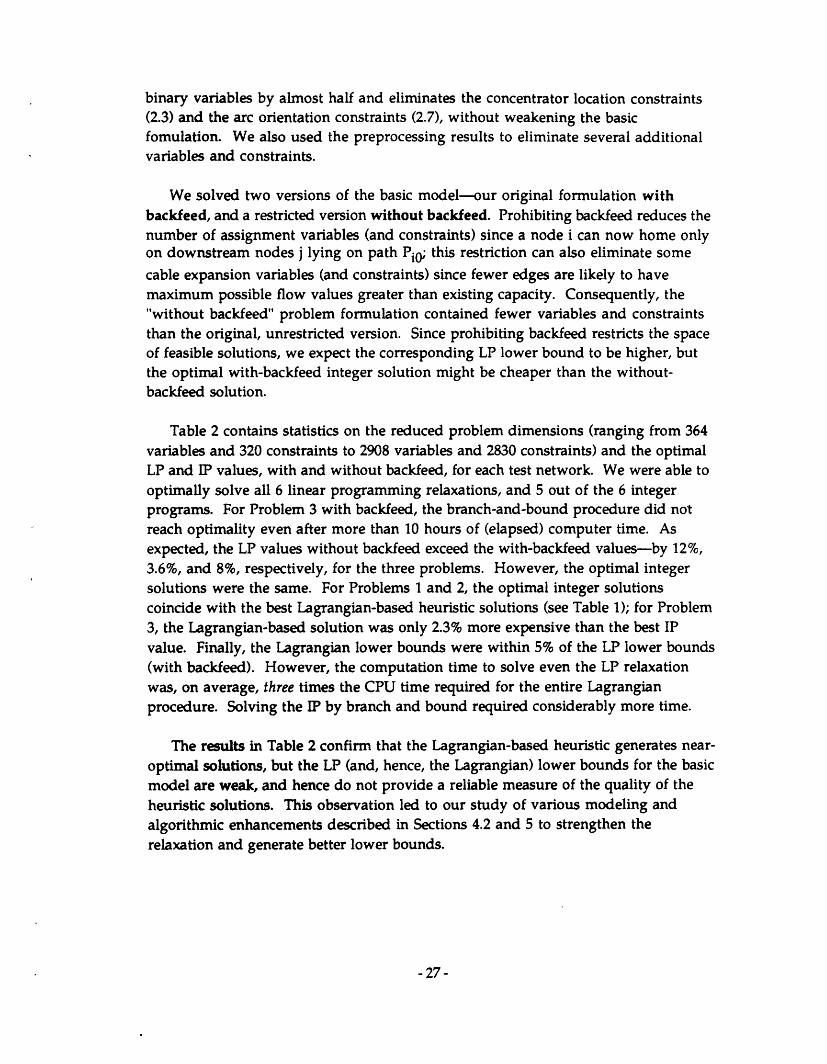
binary variables by almost half and eliminates the concentrator location constraints(2.3) and the arc orientation constraints (2.7), without weakening the basicfomulation. We also used the preprocessing results to eliminate several additionalvariables and constraints.

We solved two versions of the basic model-our original formulation withbackfeed, and a restricted version without backfeed. Prohibiting backfeed reduces thenumber of assignment variables (and constraints) since a node i can now home onlyon downstream nodes j lying on path Pi0; this restriction can also eliminate some

cable expansion variables (and constraints) since fewer edges are likely to havemaximum possible flow values greater than existing capacity. Consequently, the"without backfeed" problem formulation contained fewer variables and constraintsthan the original, unrestricted version. Since prohibiting backfeed restricts the spaceof feasible solutions, we expect the corresponding LP lower bound to be higher, butthe optimal with-backfeed integer solution might be cheaper than the without-backfeed solution.

Table 2 contains statistics on the reduced problem dimensions (ranging from 364variables and 320 constraints to 2908 variables and 2830 constraints) and the optimalLP and IP values, with and without backfeed, for each test network. We were able tooptimally solve all 6 linear programming relaxations, and 5 out of the 6 integerprograms. For Problem 3 with backfeed, the branch-and-bound procedure did notreach optimality even after more than 10 hours of (elapsed) computer time. Asexpected, the LP values without backfeed exceed the with-backfeed values-by 12%,3.6%, and 8%, respectively, for the three problems. However, the optimal integersolutions were the same. For Problems 1 and 2, the optimal integer solutionscoincide with the best Lagrangian-based heuristic solutions (see Table 1); for Problem3, the Lagrangian-based solution was only 2.3% more expensive than the best IPvalue. Finally, the Lagrangian lower bounds were within 5% of the LP lower bounds(with backfeed). However, the computation time to solve even the LP relaxationwas, on average, three times the CPU time required for the entire Lagrangianprocedure. Solving the IP by branch and bound required considerably more time.

The results in Table 2 confirm that the Lagrangian-based heuristic generates near-optimal solutions, but the LP (and, hence, the Lagrangian) lower bounds for the basicmodel are weak, and hence do not provide a reliable measure of the quality of theheuristic solutions. This observation led to our study of various modeling andalgorithmic enhancements described in Sections 4.2 and 5 to strengthen therelaxation and generate better lower bounds.

- 27-

6.3 Improved Computational ResultsWe implemented the enhanced version of our Lagrangian algorithm (Section

5.4) in the C programming language on a Macintosh II computer (with a Math co-processor). This final implementation incorporated the following features:

(i) initial heuristic solution, using local improvement on the "centralized"and "distributed" starting solutions;

(ii) problem preprocessing to eliminate variables;(iii) the Lagrangian-based heuristic with local improvement;(iv) cost-based cable expansion bounds; and,(v) the assignment-forcing, bottleneck-arc, and subtree-splitting inequalities.

We used the same subgradient settings described in Section 6.2. Table 3 containssummary statistics on the the initial upper bound, the (final) best upper and lowerbounds, the % gap, and the total computation time (elapsed time on Mac II,including time for input/output, initialization, heuristic, and subgradient iterations)for the three test problems. Again, we have scaled all the bounds for each problemwith respect to the optimal LP value.

Comparing the results of Table 1 and Table 3 highlights the dramatic reduction inthe % gap due to our enhancements-from 64%, 81%, and 124% to 1.2%, 3.2%, and7.0%, respectively, for Problems 1, 2 and 3. As before, the Lagrangian-based heuristicprocedure found the optimal solutions to Problems 1 and 2. For Problem 3, theenhancements to the Lagrangian lower bounding procedure also led to a modestimprovement (1.6%) over the previous heuristic solution (using the basic model);this improved Lagrangian-based heuristic solution is only 0.66% more expensivethan the best integer solution found using LINDO.

The order-of-magnitude reduction in the % gaps is mainly due to the vastlyimproved lower bounds. The new Lagrangian lower bounds are 60 to 95% largerthan the optimal LP values for the basic [LANI] model. These results suggest that,even though the local access network planning formulation has numerous othervalid inequalities, the cumulative effect of the few classes of cuts that we selected andimplemented far exceeds the potential effectiveness of the remaining, more complexinequalities.

Although the computation times reported in Tables 2 and 3 are notcommensurate, we estimate that general-purpose branch and bound methods mightrequire several orders of magnitude more computation time than the compositeLagrangian relaxation algorithm. Finally, we note that, even with weak lowerbounds, the Lagrangian relaxation procedure generates good starting solutions forlocal improvement. For Problems 2 and 3, the Lagrangian-based heuristic was 15 to20% cheaper than the initial heuristic solution.

- 28 -

11

6.4 Computational Results with Demand and Cost VariationsTo test the method's robustness as demand and cost parameters change, we

applied the algorithm to problem variations created by scaling the input data,holding the topology of the three networks fixed. In particular, we tested thefollowing scaled versions of each problem:

(i) Demand variation: We considered scenarios with uniformly lower or higherdemand values obtained by multiplying the original demand at each node bya common scale factor. We tested three demand scale factors: 0.5, 2.0, and 5.0;

(ii) Cable expansion cost variation: We uniformly increased or decreased thevariable cable expansion cost by a common scale factor for all edges. Wetested two values of the variable cost scale factor: 0.5 (lower variable cost), and2.0 (higher variable cost); and,

(iii) Concentrator cost variation: We increased or decreased the fixed concentratorcost (for every concentrator type) by a fixed amount at all locations. For ourtests, we considered a concentrator fixed cost increase (or decrease) equal toapproximately 50% of a type 2 concentrator's fixed cost.

Table 4 compares the computational results for the 6 variations of each problemwith the base case. For 19 out of the 21 problem instances, the % gap between theupper and lower bounds is less than 8%. The trends in the best expansion strategiesare consistent with our expectations. For instance, as demand increases,concentrators become more cost-effective, and hence the number of concentratorsincreases. Similarly, as the cable cost increases, the expansion plans tend to replacecable expansions with additional concentrators. Table 4 also illustrates that, as thedemand scale factor increases, the % gap initially increases and then declines. Withvery high demands, the existing cable capacities are negligible compared to the nodaldemands. Consequently, the total cost of an optimal "new" network, ignoringexisting cable capacities (which our dynamic program can find in a single iteration),does not differ appreciably from the optimal cost of the capacitated problem.Furthermore, as demand increases, remote homing (i.e., homing node i on anothernode j) becomes less attractive relative to local concentration, thus enabling thepreprocessing method to eliminate many assignments and strengthen theformulation (through lower cable expansion bounds).

These experiments with varying demand and cost data were intended to provideus with a broad understanding of the robustness of our solution approach. Using aformal design of experiment analysis with multiple-factor variation wouldundoubtedly provide further insight, and might even suggest additionalimprovements to our methodology.

-29-

7. Concluding Remarks

This paper has attempted to integrate three essential ingredients of contemporaryapplied integer programming research:

(1) an important practical application: Many changes in the telecommunicationsindustry-technological advances, explosive growth, capital intensivefacilities, and increasing competition-have opened new opportunities toapply sophisticated, optimization-based decision support techniques fortelecommunication network planning;

(2) decomposition methodology: Since its first successful application for solvinglarge-scale traveling salesman problems (Held and Karp [1970],[1971]),Lagrangian relaxation has become a pervasive technique for exploiting specialstructure and solving difficult, large-scale discrete optimization models; and

(3) model improvements based on polyhedral combinatorics: Motivated by theirmarked success for solving large-scale traveling salesman and many otherproblems, polyhedral techniques have become an essential building block fordesigning state-of-the-art algorithms for solving several classical integerprogramming problems.

We have demonstrated how to exploit the local access network planningproblem's special tree and routing structure, and how to integrate formulationenhancements with Lagrangian relaxation and dynamic programming. Ourcomputational results establish the effectiveness of this combined approach forsolving practical problem instances. This project also serves to highlight model-building issues such as eliciting information on common practice (e.g., the contiguityproperty) that can significantly impact algorithmic development, and the tradeoffbetween model accuracy (e.g., approximating the true concentrator costs as piecewise-linear concave functions) and solution effectiveness (time and quality).

Although our model does not consider detailed investment timing decisions andapproximates the cable and concentrator costs, we believe that it is an useful buildingblock for a practical decision support system to assist local access network planningactivities. Solving a monolithic multi-period planning model is likely to be muchmore difficult that its single-period counterpart. Instead, as Shulman and Vachani[1990] and Jack et al. [1992] suggest, we might employ an iterative framework that firstselects an end-of-horizon target network configuration, and then determines theoptimal evolution plan to reach this eventual target while meeting the demand ineach intermediate period. Our model can generate the target network at eachiteration. Comparing this iterative scheme with other multi-period planningalgorithms is an important research direction.

Modeling multiple services is another potentially fruitful area for investigation,especially in view of the anticipated diversification of services. Our model applies to

-30-

contexts where we can express the demands for different services (such as voice, data,and video) in commensurate units, and different services do not impose uniqueprocessing requirements or require different transmission media. With advancedtechnologies still under development, the structural differences between the single(aggregate) sevice model and the muliple services version is still unclear. Finally, astelephone companies transition from copper to fiber optic-based transmission in thelocal network, issues of reliability and connectivity might become more important.Because of the extremely high bandwith and vulnerability of fiber-optic networks,the focus of modeling efforts for the next generation of local access networks mightmove towards configuring reliable networks at minimum total fixed cost. Somerecent research (e.g., Groetschel, Monma, and Stoer [1992]) has shed some light onthese issues.

Acknowledgments: We wish to thank Marcia Helme, Jeffrey Musser, and AlexanderShulman for their valuable insights and modeling contributions, and for providingthe linkage with network planners in the field. Much of Richard Wong's work wascompleted at Purdue University, West Lafayette, Indiana.

-31 -

Figure 1Piecewise-Linear, Concave Cable or Concentrator Cost Function

Totalfhl9 i-

UL1 UL 212UL UL

3 4

Cable or Concentrator capacity(No. of circuits)

= Fixed (cable or concentrator) cost for technology m

= Variable (cable or concentrator) cost for technology m

= Upper limit on (cable or concentrator) throughput for technology m

FCm

VCm

ULm

II

c~

i

co

-z

IT-0 * 5(Y ;ar

a)

LO

C>

laq

P

Figure 3Reducing the Cable Expansion Bound M..

q

Totalconc. /cable

sac s

eij'1

Gijii

ci4

Concentrator costfunction

Cable Expansioncost function

Bii

-- -- r -- -

F = Fixed cost of type m concentrator at node iim

c. = Variable cost of type m concentrator at node i

Gij = Fixed cost of cable expansion on arc <i,j>

e = Variable cost of cable expansion on arc <i,j>

= Existing capacity of arc <i,j>Bij

ci2

L TU

Fi4

Fi3

Fi

Fii

Fi

III

Table 1

Computational Results for the(with Preprocessing and

Basic Lagrangian Relaxation Schemethe Local Improvement Heuristic)

% reduction = No. of assignments eliminated + total no. of possible assignments (excludingassignments to dummy nodes and from root node).

Bounds for each problem are scaled with respect to optimal value of LP relaxation (Table 2).

**

% gap = (Best Upper Bound - Best Lower Bound) /(Best Lower Bound)

§ CPU time includes time for input and initialization, subgradient iterations, and the localimprovement heuristic.

Statistic Problem 1 Problem 2 Problem 3

Number of nodes 27 25 41

No. of possible assignments* 676 441 1521% reduction in assignment variables 25% 24% 30%

Best Upper Bound using Lagrangian- 162.72 173.91 212.40based heuristict

Best Lagrangian Lower Boundt 99.25 96.15 94.91

% gap** 64% 81% 124%

CPU time (seconds on IBM 3083)5 8.4 secs 6.8 secs 22.2 secs

-"--- --_1-----

Table 2

Linear and Integer Programming Results using LINDOfor the Basic Model [LAN1]

Number of variables and constraints shown inafter preprocessing .

Objective function values for each problem arewith backfeed.

table correspond to compact formulation (Section 6.2.2)

e scaled with respect to optimal value of LP relaxation

Branch-and-bound for Problem 3 terminated, without reaching optimality, after 10 hours of elapsedtime on the IBM 3083. The table reports the value of the best incumbent at termination.

Problem 1 Problem 2 Problem 3# Nodes 27 25 41

# Variables§: Integer/Continuous 814/17 911/18 2870/38# Constraints§ 781 889 2830

Optimal Value** LP Relaxation 100.00 100.00 100.00* Integer Program 162.72 173.91 207.70 t

CPU secs (on IBM 3083)* LP Relaxation 14.2 24.3 72.9* Integer Program 307.8 691.8 t

No. of Iterations* LP Relaxation (# pivots) 384 1058 1295* Integer Prog. (# pivots/branches) 47/15898 89/56239

Without Backfeed

# Variables§: Integer / Continuous 421/5 352/12 765/24# Constraints§ 376 320 711

Optimal Value** LP Relaxation 111.98 103.63 108.02* Integer Program 162.72 173.91 207.70

CPU secs (on IBM 3083) for 2.8/36.1 4.2/72.4 6.2/2862.6LP Relaxation/Integer Program

§

Table 3

Computational Results for theEnhanced Lagrangian Relaxation Scheme

% reduction = No. of assignments eliminated + total no. of possible assignments (excludingassignments to dummy nodes and from root node).

t Bounds for each problem are scaled with respect to optimal value of LP relaxation with backfeed(Table 2).

% gap = (Best Upper Bound - Best Lower Bound) /(Best Lower Bound)

§ Computation (elapsed) time includes time for input, initialization, heuristic, and subgradientiterations.

Statistic Problem 1 Problem 2 Problem 3

Number of nodes 27 25 41

% reduction in assignment variables* 25% 24% 30%

Intial Upper Bound t 162.72 208.19 242.16

Best Upper Bound using Lagrangian- 162.72 173.91 209.08

based heuristict

Best Lagrangian Lower Boundt 160.85 168.52 195.36

% gap** 1.2% 3.2% 7.0%

Computation (elapsed) time on 285 secs 223 secs 879 secs.Mac II

X '1s ~~~Q Q

A o

h cj UN cc0 \O

0 r

O c~~cc (Z \ cn N

U U~~~~~~

~08eu , ()

cu O m O

CAO O

mC m 0- 10 cc

U o e *)

ON CO n CA

M (N (N O\t2 m LO N V

tft e t eN CD C! U o~

o o Ib o

tq X X X

Q r r LU. ci i -rA x x x

V tv a dI a) ( a)

O

(�

U Uc

C~A (A~

\O 10n \0C *nc oN

e , o10 C~ Cr~~ _~r

00U)cc

C 4O C Or-4 11:11 III

(A U) 0 U)U U U U) a) a) a)

re V U

cO c0i cc \ \

m C CO '-re el ZP e-~

U) C t U

r-4 00 a,en~ c C<U Cq

O O O UNa) a) a~ ~~) ua)10 - (NI e-- a cc ONj

O 6 N O

t O O N- Id '4 -

O O1) 0 0) 10O e'J , +

U 0 U U

U C O

(U U U UU U rd rl

(U (Id .

> wo wo

.00

JC)E.

V00

t

O'4

E:

oU0

E

,oo0

4

0 0

z0.E o -

oo

OCL)4C5E c0 Q

b. 0C Lc:

(P C

a a

. -.w

C-0

o

-

C

a,

C0 0

E

0cn

cn

a

o

C.)

x

2.

8a-0

C.U

-I

9

=

= - -

References

Aghezzaf, E. H., and L. A. Wolsey, "Modeling Piecewise Linear Concave Costs in aTree Partitioning Probelm", Working Paper, Universite Catholique de Louvain,Louvain-la-Neuve, Belgium (1990).

Balakrishnan, A., T. L. Magnanti, A. Shulman, and R. T. Wong, "Models forPlanning Capacity Expansion in Local Access Telecommunication Networks",Annals of Operations Research, Vol. 33, pp. 239-284 (1991).

Balakrishnan, A., T. L. Magnanti, and R. T. Wong, "Local AccessTelecommunication Network Expansion: Modeling and PolyhedralCharacterization", in preparation (1992).

Barany, I., J. Edmonds, and L. A. Wolsey, "Packing and Covering a Tree by Subtrees",Combinatorica, Vol. 6, pp. 221-233 (1986).

Fisher, M. L., 'The Lagrangian Relaxation Method for Solving Integer ProgrammingProblems", Management Science, Vol. 27, pp. 1-18 (1981).

Groetschel, M., C. L. Monma, and M. Stoer, "Computational Results with a CuttingPlane Algorithm for Designing Communication Networks with Low-connectivity Requirements", Operations Research, Vol. 20, pp. 309-330 (1992).

Held, M., and R. M. Karp, "The Traveling Salesman Problem and MinimumSpanning Trees", Operations Research, Vol. 18, pp. 1138-1162 (1970).

Held, M., and R. M. Karp, "The Traveling Salesman Problem and MinimumSpanning Trees: Part II", Mathematical Programming, Vol. 1, pp. 6-25 (1971).

Held, M., P. Wolfe, and H. D. Crowder, "Validation of Subgradient Optimization",Mathematical Programming, Vol. 6, pp. 62-88 (1974).

Hoffman, K. and M. W. Padberg, "LP-based Combinatorial Problem Solving",Annals of Operations Research, Vol. 4, pp. 145-194 (1985).

Jack, C., S. Kai, and A. Shulman, "NETCAP-An Interactive Optimization System forGTE Telephone Network Planning", Interfaces, Vol. 22, pp. 72-89 (1992).

Kariv, O., and S. L. Hakimi, "An Algorithmic Approach to Network LocationProblems II: The p-medians", SIAM Journal of Applied Mathematics, Vol. 27,pp. 539-560 (1979).

Nemhauser, G. and L. A. Wolsey, Integer and Combinatorial Optimization, JohnWiley & Sons, New York (1988).

Shulman, A., and R. Vachani, "An Algorithm for Capacity Expansion of Local AccessNetworks", IEEE Infocom '90, San Francisco, California (1990).

-R1 -

_ _11 __1_1_�____�___11_1__1111_1-__�---

Standard and Poor's, Industry Surveys: Telecommunications, January 23 (1992).

Wilson, Carol, "An Uncertain Future for LECs", Telephony, December 16 (1991).

-R2-