a dual conductance sensor for simultaneous measurement of
TRANSCRIPT
sensors
Article
A Dual Conductance Sensor for SimultaneousMeasurement of Void Fraction and Structure Velocityof Downward Two-Phase Flow in a SlightlyInclined Pipe
Yeon-Gun Lee 1, Woo-Youn Won 1, Bo-An Lee 2 and Sin Kim 3,*1 Department of Nuclear and Energy Engineering, Jeju National University, Jeju 63243, Korea;
[email protected] (Y.-G.L.); [email protected] (W.-Y.W.)2 Institute for Nuclear Science and Technology, Jeju National University, Jeju 63243, Korea; [email protected] School of Energy Systems Engineering, Chung-Ang University, Seoul 06974, Korea* Correspondence: [email protected]; Tel.: +82-2820-5073
Academic Editor: Vittorio M. N. PassaroReceived: 6 March 2017; Accepted: 3 May 2017; Published: 8 May 2017
Abstract: In this study, a new and improved electrical conductance sensor is proposed for applicationnot only to a horizontal pipe, but also an inclined one. The conductance sensor was designed tohave a dual layer, each consisting of a three-electrode set to obtain two instantaneous conductancesignals in turns, so that the area-averaged void fraction and structure velocity could be measuredsimultaneously. The optimum configuration of the electrodes was determined through numericalanalysis, and the calibration curves for stratified and annular flow were obtained through a seriesof static experiments. The fabricated conductance sensor was applied to a 45 mm inner diameterU-shaped downward inclined pipe with an inclination angle of 3◦ under adiabatic air-water flowconditions. In the tests, the superficial velocities ranged from 0.1 to 3.0 m/s for water and from 0.1to 18 m/s for air. The obtained mean void fraction and the structure velocity from the conductancesensor were validated against the measurement by the wire-mesh sensor and the cross-correlationtechnique for the visualized images, respectively. The results of the flow regime classification and thecorresponding time series of the void fraction at a variety of flow velocities were also discussed.
Keywords: dual conductance sensor; inclined pipe; void fraction; structure velocity; flow regime
1. Introduction
Measurement techniques for gas-liquid two-phase flows are a challenging issue in a varietyof industrial applications due to their irregular flow behavior as a result of the flow regime andcomplicated interactions between phases. In a nuclear power plant, two-phase flow is encountered inaccident conditions, and the cooling performance of safety systems to mitigate the consequences isgoverned by the flow characteristics of a water-steam mixture. The key parameters used to describe thebasic two-phase behavior include the void fraction and the flow velocity. In particular, the void fractionis a crucial variable used not only in predicting the transition of flow regimes but also heat transferand pressure drop of two-phase flows, especially by means of an empirical approach. For this reason,versatile measurement techniques have been developed and applied to two-phase flow: includingelectrical [1–11], optical [12,13], ultrasonic [14] and radiation attenuation methods [15,16] and so on.
Among the categories outlined above, the electrical impedance technique has benefits in termsof a non-intrusive insertion into flow fields, easy application to various channel shapes, fast dataacquisition rates, and convenient mobility. Classified as conductance methods and capacitance ones,the impedance technique using non-intrusive devices estimates the void fraction from measured
Sensors 2017, 17, 1063; doi:10.3390/s17051063 www.mdpi.com/journal/sensors

Sensors 2017, 17, 1063 2 of 18
electrical signals by employing a calibration curve that describes the relationship between the electricalimpedance and the volume ratio of a phase. A variety of configurations for the electrode pairshave been proposed, including the plate-, ring-, helical-, and wire-type sensors. Of the two options,conductance sensors are applicable for a conducting medium when the frequency of the AC (alternatingcurrent) excitation signal is sufficiently high, i.e., 10~100 kHz for tap water [3].
We note that the electrical signals of an electrical impedance sensor depend not only onthe area-averaged factions of a phase but also on the phase distribution inside the flow channel.The impedivity distribution within the domain can be reconstructed via Electrical ImpedanceTomography (EIT) using electric fields [4–6], but this requires a complicated inversion algorithmprocess to process a large number of data, which is fairly time-consuming. Instead, by preparing apriori the calibration curve for representative flow structures in the region of interest, the conductancesensor is easily capable of measuring spatially averaged flow properties with high frequency responses.Extensive experimental and numerical studies have been conducted in order to investigate theelectrical responses of a conductance sensor with a specific geometry, to determine the optimumconfigurations of electrodes, and to assess the capability of the proposed sensor in real multi-phaseflow conditions [3,7–9].
Recently, inspired by the prior work by De Kerpel et al. [10], Ko et al. suggested an electricalconductance sensor that employs three concave electrodes for void fraction measurement in ahorizontal pipe [11]. Using the measured conductance in the electrode pairs, the proposed sensordetermined the flow regime of a two-phase flow through predetermined criteria for flow patternclassification and successively estimated the area-averaged void fraction from a relevant calibrationcurve. The measurement accuracy for the void fraction was validated against obtained data with thewire-mesh sensor. However, the proposed sensor was able to measure only the void fraction, and itsapplication was limited to a basic horizontal pipe.
In this study, an improved electrical conductance sensor with a dual layer three-electrode setwas proposed for the first time for simultaneous measurement of the area-averaged void fraction andthe structure velocity, which is defined as the propagation velocity of the liquid-gas interface, of atwo-phase flow. In particular, the proposed sensor was aimed at being used in inclined pipes, as wellas horizontal ones. The industrial importance of the inclined pipe lies in the fact that, for a water-steammixture under condensing conditions, it provides effective means to inhibit the formation of a waterhammer by enabling effective drainage of the condensate water [17]. That is, the liquid flow is moreaccelerated in an inclined channel by the combined effect of an inclination angle and the gravitationalforce, which results in some differences in the flow structures from those in a horizontal channel. Thus,the applicability of the proposed conductance sensor to an inclined pipe needs to be evaluated.
On the basis of the numerical simulation, the electrodes configuration of each layer wasdetermined the same as the design by Ko et al. [11], and the conductance sensor with a dual layer wasfabricated. With reference to stratified, intermittent, and annular flow regimes in a downward inclinedpipe, the conductance sensor was calibrated through a series of static experiments. The conductancesensor was applied to the U-shaped pipe with an inclination of 3◦ in which an adiabatic two-phaseflow field is established, and the estimated void fraction and the structure velocity were comparedto measured results using the wire-mesh sensor and using the visualized images recorded by thehigh-speed camera, respectively.
2. Sensor Design and Verification
2.1. Mathematical Background
The fundamental concept of the proposed conductance sensor is illustrated in Figure 1. Each layerconsists of three concave electrodes arranged along the circumference of the circular pipe. Themeasured conductance between the adjacent electrode pair (electrodes A and C) is used to identify theflow regime of a two-phase flow. It takes into account the difference in the flow structures such that

Sensors 2017, 17, 1063 3 of 18
the whole circumference of the sensor will be in contact with a conductive liquid film in the annularflow, while the continuous liquid will wet partially the opposite electrode pair (electrodes A and B)without a contact to the electrode C in the stratified flow. The intermittent flow will exhibit periodicand repetitive readings of the electrical conductance by the liquid slug. Once the time-dependentelectrical signals from two successive layers of electrodes are obtained, as depicted in Figure 2, thetime lag between the layers is found through a correlation analysis to estimate the structure velocity ofa two-phase mixture, which will be discussed in detail in Section 3.1.
Sensors 2017, 17, 1063 3 of 19
2. Sensor Design and Verification
2.1. Mathematical Background
The fundamental concept of the proposed conductance sensor is illustrated in Figure 1. Each layer consists of three concave electrodes arranged along the circumference of the circular pipe. The measured conductance between the adjacent electrode pair (electrodes A and C) is used to identify the flow regime of a two-phase flow. It takes into account the difference in the flow structures such that the whole circumference of the sensor will be in contact with a conductive liquid film in the annular flow, while the continuous liquid will wet partially the opposite electrode pair (electrodes A and B) without a contact to the electrode C in the stratified flow. The intermittent flow will exhibit periodic and repetitive readings of the electrical conductance by the liquid slug. Once the time-dependent electrical signals from two successive layers of electrodes are obtained, as depicted in Figure 2, the time lag between the layers is found through a correlation analysis to estimate the structure velocity of a two-phase mixture, which will be discussed in detail in Section 3.1.
(a) (b)
Figure 1. Configuration of electrodes in the proposed conductance sensor and typical flow structures considered: (a) Annular flow condition; (b) Stratified flow condition.
Figure 2. An improved dual conductance sensor system for measurement of the structure velocity.
In an air-water two-phase flow condition, the distribution of the electrical potential within the domain is described by the generalized Laplace equation as:
( ) 0i u (1)
Figure 1. Configuration of electrodes in the proposed conductance sensor and typical flow structuresconsidered: (a) Annular flow condition; (b) Stratified flow condition.
Sensors 2017, 17, 1063 3 of 19
2. Sensor Design and Verification
2.1. Mathematical Background
The fundamental concept of the proposed conductance sensor is illustrated in Figure 1. Each layer consists of three concave electrodes arranged along the circumference of the circular pipe. The measured conductance between the adjacent electrode pair (electrodes A and C) is used to identify the flow regime of a two-phase flow. It takes into account the difference in the flow structures such that the whole circumference of the sensor will be in contact with a conductive liquid film in the annular flow, while the continuous liquid will wet partially the opposite electrode pair (electrodes A and B) without a contact to the electrode C in the stratified flow. The intermittent flow will exhibit periodic and repetitive readings of the electrical conductance by the liquid slug. Once the time-dependent electrical signals from two successive layers of electrodes are obtained, as depicted in Figure 2, the time lag between the layers is found through a correlation analysis to estimate the structure velocity of a two-phase mixture, which will be discussed in detail in Section 3.1.
(a) (b)
Figure 1. Configuration of electrodes in the proposed conductance sensor and typical flow structures considered: (a) Annular flow condition; (b) Stratified flow condition.
Figure 2. An improved dual conductance sensor system for measurement of the structure velocity.
In an air-water two-phase flow condition, the distribution of the electrical potential within the domain is described by the generalized Laplace equation as:
( ) 0i u (1)
Figure 2. An improved dual conductance sensor system for measurement of the structure velocity.
In an air-water two-phase flow condition, the distribution of the electrical potential within thedomain is described by the generalized Laplace equation as:
∇ · (σ + iωε)∇u = 0 (1)
where σ and ε denote the electrical conductivity and permittivity, respectively, and u represents theelectrical potential to be determined for each phase. In cases when the conductivity component of amedium is much larger than the permittivity, then the reactance has little influence on the impedance,and Equation (1) reduces to:
∇ · σ∇u = 0 (2)

Sensors 2017, 17, 1063 4 of 18
Then, the generalized Laplace equation for each phase of the air-water mixture is written as:
∇ · σg∇ug = 0 for gas phase (3a)
∇ · σl∇ul = 0 for liquid phase (3b)
If the current I flows between the electrodes of the sensor when the applied voltage difference isequal to ∆V, the electrical conductance is expressed as G = I/∆V. In order to normalize the electricalconductance in a variety of sizes of sensors, a dimensionless conductance can be introduced as follows:
G∗ =GGl
(4)
where Gl denotes the measured conductance value between the electrodes when the measurementdomain is completely filled with the liquid at an ambient temperature, and thus the void fractionis zero.
2.2. Numerical Calculations for Sensor Design
The circumferential size of electrodes and the gap between them were determined by solvingnumerically Equation (3) in a circular domain. In this study, 3-D numerical calculation based onthe finite element method was conducted using COMSOL Multiphysics. The angular gap betweenelectrodes A and B in the bottom was denoted as θ1, and the circumferential size of the electrode Cand the angle between electrodes at the top were represented as θ2 and θ3, respectively. They weredetermined by the requirement that the non-linearity error for the void fraction measurement beminimized in order to obtain a linear response to the variations of the gas or liquid volume fraction.The non-linearity error was defined as:
η =∣∣∣G∗linear − G∗opp
∣∣∣max× 100 (%) (5)
where G∗linear indicates the linear conductance, which has the same value as the liquid volume fraction,and G∗opp means the calculated dimensionless conductance between the opposite electrodes A and Bfor a given void fraction and geometrical parameters.
The numerical calculations reproduced the typical interfacial structure for the annular and thestratified flow regimes, and a wide range of the void fraction for each flow pattern was covered. Theelectrical properties of the medium and the dimension of the sensor used in the computation weresummarized in Table 1. From the calculation results, the optimized design for the three-electrodesensor was decided as θ1 = 0.5 rad, θ2 = 0.2 rad, and θ3 = 0.3 rad. The non-linearity error was 5.7% forthe annular flow, and 12.7% for the stratified flow. See Ko et al. [11] for details of simulation results.
Table 1. Electrical properties and sensor dimensions for the numerical calculation.
Variables Value
Conductivity (S/m)
Water 0.005Air 0Electrode 1.0 × 10⁶
Gap 0
Applied voltage (V) 5Signal frequency (kHz) 10Inner diameter of the sensor (mm) 45Width of electrodes (De, mm) 15Dimensionless gap size (Dg/De) 0.25~5

Sensors 2017, 17, 1063 5 of 18
Another crucial parameter to be determined is the spacing between the electrode layers. If theyare positioned too close, the electrodes in one layer may interfere with the measured electrical signalsof another layer. On the contrary, when they are far apart from each other, the flow structure mayvary substantially between them and the accuracy of the velocity measurement might be reduced.In order to determine a minimum distance that excludes the electrical interferences between layers,the variation of the conductance with the spacing between the layers was numerically simulated.The deviation from the dimensionless conductance for a single-layered sensor according to the spacingwas plotted in Figure 3. Note that the X-axis of Figure 3 indicates the dimensionless spacing (Dg/De)defined as the spacing (Dg) divided by the width of the electrode (De), 15 mm. The simulations werecarried out with regard to two flow conditions: two-phase conditions with the void fraction of 0.8 and0.5 in the annular and stratified flows, respectively.
Sensors 2017, 17, 1063 5 of 19
Table 1. Electrical properties and sensor dimensions for the numerical calculation.
Variables Value
Conductivity (S/m)
Water 0.005 Air 0 Electrode 1.0 × 10⁶ Gap 0
Applied voltage (V) 5 Signal frequency (kHz) 10 Inner diameter of the sensor (mm) 45 Width of electrodes (De, mm) 15 Dimensionless gap size (Dg/De) 0.25~5
Another crucial parameter to be determined is the spacing between the electrode layers. If they are positioned too close, the electrodes in one layer may interfere with the measured electrical signals of another layer. On the contrary, when they are far apart from each other, the flow structure may vary substantially between them and the accuracy of the velocity measurement might be reduced. In order to determine a minimum distance that excludes the electrical interferences between layers, the variation of the conductance with the spacing between the layers was numerically simulated. The deviation from the dimensionless conductance for a single-layered sensor according to the spacing was plotted in Figure 3. Note that the X-axis of Figure 3 indicates the dimensionless spacing (Dg/De) defined as the spacing (Dg) divided by the width of the electrode (De), 15 mm. The simulations were carried out with regard to two flow conditions: two-phase conditions with the void fraction of 0.8 and 0.5 in the annular and stratified flows, respectively.
0.0 0.5 1.0 1.5 2.0 2.5 3.0 3.5 4.0 4.5 5.00.85
0.90
0.95
1.00
1.05
1.10
1.15
Dim
ensio
nles
s con
duct
ance
(G*)
Dimensionless gap size (Dg/De)
Annular (=0.8) Stratified (=0.5)
Deviation of G* < 0.01
Figure 3. Variation of the calculated conductance according to the spacing between layers.
Inspection of Figure 3 revealed that the conductance sensor suffered from electrical interferences under single-phase liquid or stratified flow conditions as the spacing became narrow while the electrical conductance was rarely influenced by the annular flow spacing. As the dimensionless spacing of the dual sensor increases, the deviation from the conductance calculated for a single-layered sensor diminishes. The deviation of the dimensionless conductance was reduced below 1% when the dimensionless spacing was not less than 2.0. From the numerical results, the distance between the electrodes layers was determined to be 30 mm. For other diameters or inclination angles of a pipe, the design of the conductance sensor can be determined in the same way as the above mentioned optimization process. Depending on the flow structures in a targeted near-horizontal pipe, the configuration may be altered from the present one a little.
Figure 3. Variation of the calculated conductance according to the spacing between layers.
Inspection of Figure 3 revealed that the conductance sensor suffered from electrical interferencesunder single-phase liquid or stratified flow conditions as the spacing became narrow while theelectrical conductance was rarely influenced by the annular flow spacing. As the dimensionlessspacing of the dual sensor increases, the deviation from the conductance calculated for a single-layeredsensor diminishes. The deviation of the dimensionless conductance was reduced below 1% when thedimensionless spacing was not less than 2.0. From the numerical results, the distance between theelectrodes layers was determined to be 30 mm. For other diameters or inclination angles of a pipe,the design of the conductance sensor can be determined in the same way as the above mentionedoptimization process. Depending on the flow structures in a targeted near-horizontal pipe, theconfiguration may be altered from the present one a little.
2.3. Verification
The electrical conductance sensor was fabricated based on the optimized design throughthe numerical calculations. The details of the sensor configurations are summarized in Table 2.The electrodes were flush-mounted on the inner wall of a short acrylic pipe unit.

Sensors 2017, 17, 1063 6 of 18
Table 2. Details of the optimized sensor configurations.
Variables Value
Circumferential size (rad)Electrode A & B 2.54Electrode C 0.30
Inner diameter of the sensor (mm) 45Width of electrodes (De, mm) 15Thickness of electrodes (mm) 2 (concave)Spacing between layers (mm) 30
The measurement accuracy of the fabricated dual conductance sensor was verified through aseries of static experiments. The fractions of a phase inside a horizontal pipe were adjusted withstagnant water and acrylic rods and the linearity degree of the measured electrical conductance wascompared to the predictions of numerical calculations. In simulating the annular flow, an acrylic rodwhose diameter corresponds to a prescribed void fraction was placed at the center of the channel filledwith water. The void fraction in the stratified flow was set by introducing known water volumes insidethe horizontal pipe. The potential difference of 5 V was imposed to a pair of opposite electrodes Aand B, and the frequency of the applied signal was set to 10 kHz. Refer to Section 3.2 for detailedinformation of the measurement system. The static experiments were performed for the void fraction inthe ranges between 0.4 and 1.0 for the annular flow, and 0.0 and 1.0 for the stratified flow, respectively.Figure 4 presents the measured dimensionless conductance according to the void fraction, and thecomparison results with the numerically obtained curve.
Sensors 2017, 17, 1063 6 of 19
2.3. Verification
The electrical conductance sensor was fabricated based on the optimized design through the numerical calculations. The details of the sensor configurations are summarized in Table 2. The electrodes were flush-mounted on the inner wall of a short acrylic pipe unit.
Table 2. Details of the optimized sensor configurations.
Variables Value
Circumferential size (rad) Electrode A & B 2.54 Electrode C 0.30
Inner diameter of the sensor (mm) 45 Width of electrodes (De, mm) 15 Thickness of electrodes (mm) 2 (concave) Spacing between layers (mm) 30
The measurement accuracy of the fabricated dual conductance sensor was verified through a series of static experiments. The fractions of a phase inside a horizontal pipe were adjusted with stagnant water and acrylic rods and the linearity degree of the measured electrical conductance was compared to the predictions of numerical calculations. In simulating the annular flow, an acrylic rod whose diameter corresponds to a prescribed void fraction was placed at the center of the channel filled with water. The void fraction in the stratified flow was set by introducing known water volumes inside the horizontal pipe. The potential difference of 5 V was imposed to a pair of opposite electrodes A and B, and the frequency of the applied signal was set to 10 kHz. Refer to Section 3.2 for detailed information of the measurement system. The static experiments were performed for the void fraction in the ranges between 0.4 and 1.0 for the annular flow, and 0.0 and 1.0 for the stratified flow, respectively. Figure 4 presents the measured dimensionless conductance according to the void fraction, and the comparison results with the numerically obtained curve.
(a) (b)
Figure 4. Predicted and measured dimensionless conductance as a function of the void fraction: (a) Annular flow; (b) Stratified flow.
The profile of the dimensionless conductance exhibited a non-linear pattern with the variation of the void fraction. For both flow regimes, the measurements and the numerical value were in very close agreement over the void fraction range investigated. The measured non-linearity error was 7.0% for the annular flow, and 12% for the stratified flow, which were similar to those from numerical calculations. This demonstrated the adopted approach was reliable, and the conductance sensor was fabricated well following the intended design. The measured conductance data were then used in a form of the look-up table to determine the void fraction in subsequent flow conditions.
0 0.2 0.4 0.6 0.8 1
Void fraction,
0
0.2
0.4
0.6
0.8
1Numerical solutionExperiments
0 0.2 0.4 0.6 0.8 1
Void fraction,
0
0.2
0.4
0.6
0.8
1Numerical solutionExperiments
Figure 4. Predicted and measured dimensionless conductance as a function of the void fraction:(a) Annular flow; (b) Stratified flow.
The profile of the dimensionless conductance exhibited a non-linear pattern with the variationof the void fraction. For both flow regimes, the measurements and the numerical value were in veryclose agreement over the void fraction range investigated. The measured non-linearity error was7.0% for the annular flow, and 12% for the stratified flow, which were similar to those from numericalcalculations. This demonstrated the adopted approach was reliable, and the conductance sensor wasfabricated well following the intended design. The measured conductance data were then used in aform of the look-up table to determine the void fraction in subsequent flow conditions.
Sensors 2017, 17, 1063 7 of 18
3. Experiments
3.1. Measurement Techniques
3.1.1. Measurement of Void Fraction
In order to evaluate the void fraction of a two-phase flow using the conductance sensor, theflow pattern in the channel has to be identified at first. The flow patterns in a slightly inclined pipeare divided roughly into three conditions: stratified, intermittent, and annular flows. By takinginto account typical flow patterns inside the flow channel and characteristics of correspondingelectrical signals from three electrodes, one can distinguish the flow pattern established throughthe conductance sensor.
In a stratified flow, the phases are separated by the density difference. Thus water occupies thelower section of the cross-sectional height of the pipe while steam or air flows floating on water. As thehighly conductive liquid rarely makes contact to the electrode C on the top of the flow channel, thedimensionless conductance measured between the adjacent electrodes A and C (G∗adj) are very small.The static experiment revealed that the measured value in a simulated stratified flow condition wasless than 0.005, which corresponded to the measurement error of the LCR meter used in the test.In actual flow conditions, however, dispersed water droplets or an incomplete liquid film around theperiphery may affect the measured conductance. Thus, the upper threshold of G∗adj to identify thestratified flow was determined to 0.01.
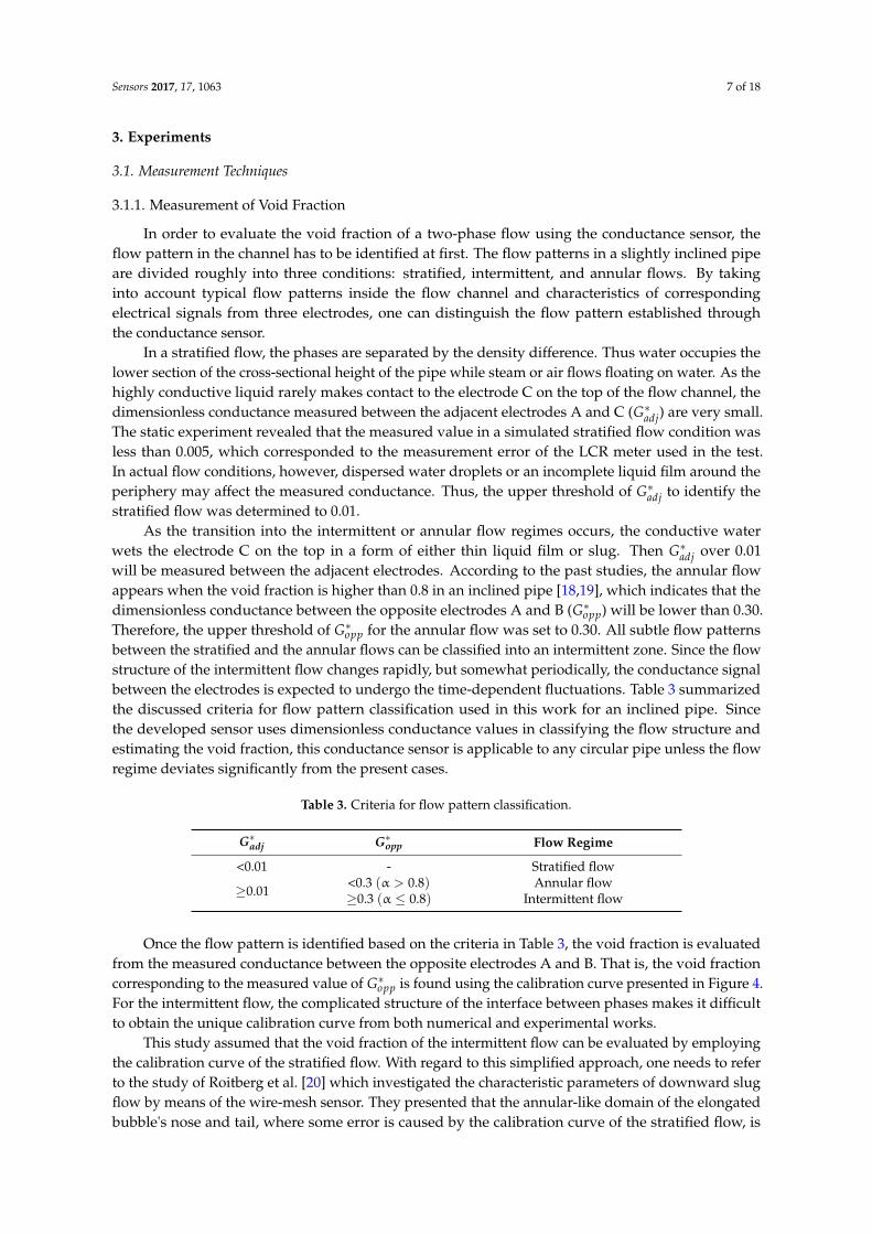
As the transition into the intermittent or annular flow regimes occurs, the conductive waterwets the electrode C on the top in a form of either thin liquid film or slug. Then G∗adj over 0.01will be measured between the adjacent electrodes. According to the past studies, the annular flowappears when the void fraction is higher than 0.8 in an inclined pipe [18,19], which indicates that thedimensionless conductance between the opposite electrodes A and B (G∗opp) will be lower than 0.30.Therefore, the upper threshold of G∗opp for the annular flow was set to 0.30. All subtle flow patternsbetween the stratified and the annular flows can be classified into an intermittent zone. Since the flowstructure of the intermittent flow changes rapidly, but somewhat periodically, the conductance signalbetween the electrodes is expected to undergo the time-dependent fluctuations. Table 3 summarizedthe discussed criteria for flow pattern classification used in this work for an inclined pipe. Sincethe developed sensor uses dimensionless conductance values in classifying the flow structure andestimating the void fraction, this conductance sensor is applicable to any circular pipe unless the flowregime deviates significantly from the present cases.
Table 3. Criteria for flow pattern classification.
G∗adj G∗opp Flow Regime
<0.01 - Stratified flow
≥0.01<0.3 (α > 0.8) Annular flow≥0.3 (α ≤ 0.8) Intermittent flow
Once the flow pattern is identified based on the criteria in Table 3, the void fraction is evaluatedfrom the measured conductance between the opposite electrodes A and B. That is, the void fractioncorresponding to the measured value of G∗opp is found using the calibration curve presented in Figure 4.For the intermittent flow, the complicated structure of the interface between phases makes it difficultto obtain the unique calibration curve from both numerical and experimental works.
This study assumed that the void fraction of the intermittent flow can be evaluated by employingthe calibration curve of the stratified flow. With regard to this simplified approach, one needs to referto the study of Roitberg et al. [20] which investigated the characteristic parameters of downward slugflow by means of the wire-mesh sensor. They presented that the annular-like domain of the elongatedbubble's nose and tail, where some error is caused by the calibration curve of the stratified flow, is

Sensors 2017, 17, 1063 8 of 18
much shorter in length than the stratified-like domain of bubble’s body and liquid slug. Thus, eventhough not perfect, applying the calibration curve of the stratified flow to the intermittent flow regimedoes not cause significant error in the void fraction measurement.
3.1.2. Measurement of Structure Velocity
The structure velocity of a two-phase flow is evaluated by the cross-correlation analysis oftwo area-averaged void fraction time series obtained from the dual conductance sensor. From thetime-varying void fraction records, one finds the time-shift that maximizes the Pearson correlationcoefficient; it describes the degree to which two parameters are linearly correlated. The Pearsoncorrelation coefficient gives values between 1 and −1, where a value of 1 implies a perfect linearrelationship between parameters, and 0 indicates no linear correlation. As the time series of voidfraction signals are obtained from two successive layers of the electrodes, the time lag elapsed fora two-phase flow to move between the layers is determined by the requirement that the correlationcoefficient be maximum. Then the structure velocity of a two-phase flow is calculated as follows:
jsv =Dg
∆t(6)
where Dg is the spacing between the layers (30 mm in this study), and ∆t is the time lag that givesthe maximum cross-correlation coefficient. Note that the velocity by Equation (6) is not a phasicvelocity, but the propagation velocity of the interfacial structures between phases [21]. For example, thestructure velocity corresponds to the propagation velocity of the periodic surface of liquid disturbancewaves for the stratified-wavy flow, and that of highly unstable films for the annular flow. For theslug or elongated bubbles flow, it corresponds to the velocity of the large gas bubbles since the phasicfraction in the flow channel is determined by them. Note that this structure velocity is governed by thebulk structure of the phases, and the dispersed phase affects little to it. By the principle, the velocitymeasurements with this conductance sensor are limited to the axial direction of the pipe.
3.2. Experimental Setup
Illustrated in Figure 5 is the schematic diagram of the air-water two-phase flow loop at JejuNational University. This experimental facility consists of the main tank, the main pump, the preheater,the air compressor, the test section, and the separator. The flow rate of the supplied water to the testsection is controlled by the main pump, and measured by the Coriolis flowmeter installed downstreamof the main pump. The compressed air is supplied to the injector located near the entrance of the testsection and mixed with water. Its flow rate is also measured by the Coriolis flowmeter. After flowingthrough the test section, a two-phase mixture is separated at the collection tank where air is dischargedto the atmosphere and water is recirculated to the main tank.
The test section is the U-shaped inclined pipe with an inclination angle of 3◦. The test section wasconstructed to simulate the heat exchanger of the Passive Auxiliary Feedwater System (PAFS) adoptedin a next-generation Korean nuclear power plant, APR+ (Advanced Power Reactor Plus). It removespassively the decay heat from the reactor core by condensing steam from the steam generator inside aheat exchanger submerged in a large pool [22].
To prevent the occurrence of a condensation-induced water hammer inside the tube, the heatexchanger was designed to be inclined at 3◦. The test section of the experimental facility is made fromacrylic pipes to enable visual observation of a two-phase flow inside the flow channel. It is 44.8 mmin inner diameter, and 7246 mm in total length including the bend. The length of the straight testsection is 3218 mm. The air-water two-phase mixture flows downward along this slightly inclinedpipe. The proposed conductance sensor was placed at a distance 2500 mm from the entrance of the testsection (L/D = 55). A photograph of the dual conductance sensor installed in the test section is shownin Figure 6.

Sensors 2017, 17, 1063 9 of 18Sensors 2017, 17, 1063 9 of 19
Figure 5. Schematic diagram of the air-water two-phase flow loop.
To prevent the occurrence of a condensation-induced water hammer inside the tube, the heat exchanger was designed to be inclined at 3°. The test section of the experimental facility is made from acrylic pipes to enable visual observation of a two-phase flow inside the flow channel. It is 44.8 mm in inner diameter, and 7246 mm in total length including the bend. The length of the straight test section is 3218 mm. The air-water two-phase mixture flows downward along this slightly inclined pipe. The proposed conductance sensor was placed at a distance 2500 mm from the entrance of the test section (L/D = 55). A photograph of the dual conductance sensor installed in the test section is shown in Figure 6.
Figure 6. Schematic diagram of the air-water two-phase flow loop.
Figure 7 presents the schematic diagram of the measurement system for the conductance sensor. An AC voltage was applied via a 4284A LCR meter (Agilent technologies, Santa Clara, CA, USA) to a pair of electrodes. The switch module (NI PXI-2536, National Instruments, Austin, TX, USA) then opened and closed alternatively the circuits connected to the opposite and the adjacent pairs of electrodes, respectively. A shunt resistor was connected in parallel between the electrode and the switch module. The voltage difference across the resistor was measured by a DAQ unit (NI PXI-6368, National Instruments, Austin, TX, USA) and converted to the current signal. Detailed specifications of the devices used in the measurement are shown in Table 4. The collected conductance signal passing through the circuit was processed in real time to calculate the void fraction according to the results of the flow regime classification.
Figure 5. Schematic diagram of the air-water two-phase flow loop.
Sensors 2017, 17, 1063 9 of 19
Figure 5. Schematic diagram of the air-water two-phase flow loop.
To prevent the occurrence of a condensation-induced water hammer inside the tube, the heat exchanger was designed to be inclined at 3°. The test section of the experimental facility is made from acrylic pipes to enable visual observation of a two-phase flow inside the flow channel. It is 44.8 mm in inner diameter, and 7246 mm in total length including the bend. The length of the straight test section is 3218 mm. The air-water two-phase mixture flows downward along this slightly inclined pipe. The proposed conductance sensor was placed at a distance 2500 mm from the entrance of the test section (L/D = 55). A photograph of the dual conductance sensor installed in the test section is shown in Figure 6.
Figure 6. Schematic diagram of the air-water two-phase flow loop.
Figure 7 presents the schematic diagram of the measurement system for the conductance sensor. An AC voltage was applied via a 4284A LCR meter (Agilent technologies, Santa Clara, CA, USA) to a pair of electrodes. The switch module (NI PXI-2536, National Instruments, Austin, TX, USA) then opened and closed alternatively the circuits connected to the opposite and the adjacent pairs of electrodes, respectively. A shunt resistor was connected in parallel between the electrode and the switch module. The voltage difference across the resistor was measured by a DAQ unit (NI PXI-6368, National Instruments, Austin, TX, USA) and converted to the current signal. Detailed specifications of the devices used in the measurement are shown in Table 4. The collected conductance signal passing through the circuit was processed in real time to calculate the void fraction according to the results of the flow regime classification.
Figure 6. Schematic diagram of the air-water two-phase flow loop.
Figure 7 presents the schematic diagram of the measurement system for the conductance sensor.An AC voltage was applied via a 4284A LCR meter (Agilent technologies, Santa Clara, CA, USA)to a pair of electrodes. The switch module (NI PXI-2536, National Instruments, Austin, TX, USA)then opened and closed alternatively the circuits connected to the opposite and the adjacent pairsof electrodes, respectively. A shunt resistor was connected in parallel between the electrode and theswitch module. The voltage difference across the resistor was measured by a DAQ unit (NI PXI-6368,National Instruments, Austin, TX, USA) and converted to the current signal. Detailed specifications ofthe devices used in the measurement are shown in Table 4. The collected conductance signal passingthrough the circuit was processed in real time to calculate the void fraction according to the results ofthe flow regime classification.
Table 4. Specifications of measurement instruments used for experiments.
Instruments Accuracy Signal Range Time Definition
Agilent 4284A LCR meter 0.05~0.5% Up to 20 V with 1 MHz N/ANI PXI-2536 N/A Up to ±12 V and 100 mA 5 × 10⁴ cross-points/sNI PXIe-6368 3 mV for ±10 V range Up to ±10 V 2 × 10⁶ samples/channel

Sensors 2017, 17, 1063 10 of 18Sensors 2017, 17, 1063 10 of 19
Figure 7. Measurement system for the conductance sensor.
Table 4. Specifications of measurement instruments used for experiments.
Instruments Accuracy Signal Range Time Definition
Agilent 4284A LCR meter 0.05~0.5% Up to 20 V with 1 MHz N/A
NI PXI-2536 N/A Up to ±12 V and 100 mA 5 × 10⁴ cross-points/s
NI PXIe-6368 3 mV for ±10 V
range Up to ±10 V
2 × 10⁶ samples/channel
The applied voltage was set to 5 V with a signal frequency of 10 kHz to ensure that the impedance response became conductive. As the evaluation of the flow pattern and the void fraction was carried out alternatively during the switching frequency, the maximum measurement speed of the proposed conductance sensor was 5000 fps. In the experiment, it was adjusted to 500 fps in consideration of the accuracy of the data acquisition. The switching speed and the sampling rate was set to 2 kHz and 2000 kps, respectively.
3.3. Test Matrix
The developed conductance sensor system was applied to a series of the air-water two-phase flow experiments. A wide variety of superficial velocities ranging from 0.1 to 3.0 m/s for water and from 0.1 to 18 m/s for air were tested. Some selected flow conditions discussed herein are summarized in Table 5, and marked on the flow regime map by Taitel and Dukler [23] for near horizontal two-phase flows in Figure 8. The fluid temperature was kept constant at an ambient temperature of 22 °Cto 24 °C during the experiments. Due to the limited capacity of the air compressor used in this experiment, a complete form of an annular flow could not be established; however, one expected the sporadic appearance of an annular liquid film around the periphery of the flow channel in the intermittent flow conditions.
Figure 7. Measurement system for the conductance sensor.
The applied voltage was set to 5 V with a signal frequency of 10 kHz to ensure that the impedanceresponse became conductive. As the evaluation of the flow pattern and the void fraction was carriedout alternatively during the switching frequency, the maximum measurement speed of the proposedconductance sensor was 5000 fps. In the experiment, it was adjusted to 500 fps in consideration of theaccuracy of the data acquisition. The switching speed and the sampling rate was set to 2 kHz and2000 kps, respectively.
3.3. Test Matrix
The developed conductance sensor system was applied to a series of the air-water two-phase flowexperiments. A wide variety of superficial velocities ranging from 0.1 to 3.0 m/s for water and from0.1 to 18 m/s for air were tested. Some selected flow conditions discussed herein are summarized inTable 5, and marked on the flow regime map by Taitel and Dukler [23] for near horizontal two-phaseflows in Figure 8. The fluid temperature was kept constant at an ambient temperature of 22 ◦C to 24 ◦Cduring the experiments. Due to the limited capacity of the air compressor used in this experiment,a complete form of an annular flow could not be established; however, one expected the sporadicappearance of an annular liquid film around the periphery of the flow channel in the intermittentflow conditions.
Table 5. Test matrix for air-water two-phase flow experiments in the inclined loop.
Run jl (m/s) jg (m/s) Flow Pattern “by Map”
1~5 0.1 0.1, 0.5, 1, 5, 10, 12 Stratified flow6 0.3 18 Annular low
7~11 0.50.1, 0.5, 1, 5, 10, 12
Stratified flow12~16 1 Intermittent flow17~21 2 Intermittent flow22~25 3 0.1, 0.5, 1, 10 Intermittent flow
Sensors 2017, 17, 1063 11 of 18
Sensors 2017, 17, 1063 11 of 19
Table 5. Test matrix for air-water two-phase flow experiments in the inclined loop.
Run jl (m/s) jg (m/s) Flow Pattern “by Map”
1~5 0.1 0.1, 0.5, 1, 5, 10, 12 Stratified flow
6 0.3 18 Annular low
7~11 0.5
0.1, 0.5, 1, 5, 10, 12
Stratified flow
12~16 1 Intermittent flow
17~21 2 Intermittent flow
22~25 3 0.1, 0.5, 1, 10 Intermittent flow
4. Results and Discussion
4.1. Validation
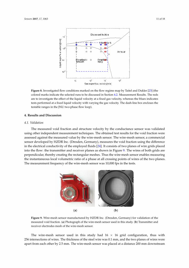
The measured void fraction and structure velocity by the conductance sensor was validated using other independent measurement techniques. The obtained test results for the void fraction were assessed against the measured value by the wire-mesh sensor. The wire-mesh sensor, a commercial sensor developed by HZDR Inc. (Dresden, Germany), measures the void fraction using the difference in the electrical conductivity of the employed fluids [24]. It consists of two planes of wire grids placed into the flow: the transmitter and receiver planes as shown in Figure 9. The wires of both grids are perpendicular, thereby creating the rectangular meshes. Thus the wire-mesh sensor enables measuring the instantaneous local volumetric ratio of a phase at all crossing points of wires of the two planes. The measurement frequency of the wire-mesh sensor was 10,000 fps in the tests.
Figure 8. Investigated flow conditions marked on the flow regime map by Taitel and Dukler [23] (the colored marks indicate the selected runs to be discussed in Section 4.2. Measurement Results. The reds are to investigate the effect of the liquid velocity at a fixed gas velocity, whereas the blues indicates tests performed at a fixed liquid velocity with varying the gas velocity. The dash-line box encloses the testable ranges in the JNU two-phase flow loop).
The wire-mesh sensor used in this study had 16 × 16 grid configuration, thus with 256 intersections of wires. The thickness of the steel wire was 0.1 mm, and the two planes of wires were apart from each other by 2.5 mm. The wire-mesh sensor was placed at a distance 200 mm downstream from the conductance sensor. This spacing was the best compromise obtained from the numerical simulation to exclude the influence of electrical interferences between the sensors and to minimize the variation in the phase distribution while passing through both sensors.
Figure 8. Investigated flow conditions marked on the flow regime map by Taitel and Dukler [23] (thecolored marks indicate the selected runs to be discussed in Section 4.2. Measurement Results. The redsare to investigate the effect of the liquid velocity at a fixed gas velocity, whereas the blues indicatestests performed at a fixed liquid velocity with varying the gas velocity. The dash-line box encloses thetestable ranges in the JNU two-phase flow loop).
4. Results and Discussion
4.1. Validation
The measured void fraction and structure velocity by the conductance sensor was validatedusing other independent measurement techniques. The obtained test results for the void fraction wereassessed against the measured value by the wire-mesh sensor. The wire-mesh sensor, a commercialsensor developed by HZDR Inc. (Dresden, Germany), measures the void fraction using the differencein the electrical conductivity of the employed fluids [24]. It consists of two planes of wire grids placedinto the flow: the transmitter and receiver planes as shown in Figure 9. The wires of both grids areperpendicular, thereby creating the rectangular meshes. Thus the wire-mesh sensor enables measuringthe instantaneous local volumetric ratio of a phase at all crossing points of wires of the two planes.The measurement frequency of the wire-mesh sensor was 10,000 fps in the tests.
Sensors 2017, 17, 1063 12 of 19
The structure velocity measured by the conductance sensor was validated using the visualized images recorded by the high-speed camera. Figure 10 illustrates the process to estimate the structure velocity by the high-speed camera measurement technique. The flow field inside the inclined pipe was visualized from the side using back-lighting, which created the shadow along the interfaces of air bubbles. Then the boundaries between phases were discriminated precisely by the Sobel edge detection scheme provided by the image analysis tool, MATLAB (MathWorks, Natick, MA, USA) (Figure 10b). The local brightness of the processed image was determined by the phase distribution. Then, one divided finely the entire image into the flow direction to set the regions of interest and calculated the sum of values of brightness in each area so that their profile across the image could be plotted as the blue line in Figure 10c. The same process was repeated for the image captured after a few frames, and then almost the same transversal profile of the sum of brightness can be extracted with a slight shift in distance. By applying the cross-correlation technique to two consecutive images information, one can trace the moving distance of the interfaces during a constant time interval.
(a) (b)
Figure 9. Wire-mesh sensor manufactured by HZDR Inc. (Dresden, Germany) for validation of the measured void fraction. (a) Photograph of the wire-mesh sensor used in this study. (b) Transmitter and receiver electrodes mesh of the wire-mesh sensor
Figure 10. Cross-correlation method using the visualized images for verification of the measured structure velocity. (a) Visualized image recorded by the high-speed camera. (b) Phase edge detection applied to two images captured with a known time interval. (c) Distributions of the brightness integrated by column. (d) Shift in distance determined by the cross-correlation analysis for the best match of the brightness distributions.
The procedure mentioned above was applied to a couple of pairs of sequential images to estimate the average structure velocity of a two-phase flow. In short, this high-speed camera
0 20 40 60 80 100 120 140 160
column number
0.5
1
1.5
2
2.5
3
3.5
Inte
nsity
of e
ach
co
lum
n
104
f irst imagesecond image
0 20 40 60 80 100 120 140 160
column number
0.5
1
1.5
2
2.5
3
3.5
Inte
nsi
ty o
f ea
ch c
olu
mn
104
f irst imagesecond image
(a) (b)
(c)(d)
Image processing
Cross-correlationanalysis
Profile of brightness
Figure 9. Wire-mesh sensor manufactured by HZDR Inc. (Dresden, Germany) for validation of themeasured void fraction. (a) Photograph of the wire-mesh sensor used in this study. (b) Transmitter andreceiver electrodes mesh of the wire-mesh sensor.
The wire-mesh sensor used in this study had 16 × 16 grid configuration, thus with256 intersections of wires. The thickness of the steel wire was 0.1 mm, and the two planes of wires wereapart from each other by 2.5 mm. The wire-mesh sensor was placed at a distance 200 mm downstream

Sensors 2017, 17, 1063 12 of 18
from the conductance sensor. This spacing was the best compromise obtained from the numericalsimulation to exclude the influence of electrical interferences between the sensors and to minimize thevariation in the phase distribution while passing through both sensors.
The structure velocity measured by the conductance sensor was validated using the visualizedimages recorded by the high-speed camera. Figure 10 illustrates the process to estimate the structurevelocity by the high-speed camera measurement technique. The flow field inside the inclined pipewas visualized from the side using back-lighting, which created the shadow along the interfaces ofair bubbles. Then the boundaries between phases were discriminated precisely by the Sobel edgedetection scheme provided by the image analysis tool, MATLAB (MathWorks, Natick, MA, USA)(Figure 10b). The local brightness of the processed image was determined by the phase distribution.Then, one divided finely the entire image into the flow direction to set the regions of interest andcalculated the sum of values of brightness in each area so that their profile across the image could beplotted as the blue line in Figure 10c. The same process was repeated for the image captured after afew frames, and then almost the same transversal profile of the sum of brightness can be extractedwith a slight shift in distance. By applying the cross-correlation technique to two consecutive imagesinformation, one can trace the moving distance of the interfaces during a constant time interval.
Sensors 2017, 17, 1063 12 of 19
The structure velocity measured by the conductance sensor was validated using the visualized images recorded by the high-speed camera. Figure 10 illustrates the process to estimate the structure velocity by the high-speed camera measurement technique. The flow field inside the inclined pipe was visualized from the side using back-lighting, which created the shadow along the interfaces of air bubbles. Then the boundaries between phases were discriminated precisely by the Sobel edge detection scheme provided by the image analysis tool, MATLAB (MathWorks, Natick, MA, USA) (Figure 10b). The local brightness of the processed image was determined by the phase distribution. Then, one divided finely the entire image into the flow direction to set the regions of interest and calculated the sum of values of brightness in each area so that their profile across the image could be plotted as the blue line in Figure 10c. The same process was repeated for the image captured after a few frames, and then almost the same transversal profile of the sum of brightness can be extracted with a slight shift in distance. By applying the cross-correlation technique to two consecutive images information, one can trace the moving distance of the interfaces during a constant time interval.
(a) (b)
Figure 9. Wire-mesh sensor manufactured by HZDR Inc. (Dresden, Germany) for validation of the measured void fraction. (a) Photograph of the wire-mesh sensor used in this study. (b) Transmitter and receiver electrodes mesh of the wire-mesh sensor
Figure 10. Cross-correlation method using the visualized images for verification of the measured structure velocity. (a) Visualized image recorded by the high-speed camera. (b) Phase edge detection applied to two images captured with a known time interval. (c) Distributions of the brightness integrated by column. (d) Shift in distance determined by the cross-correlation analysis for the best match of the brightness distributions.
The procedure mentioned above was applied to a couple of pairs of sequential images to estimate the average structure velocity of a two-phase flow. In short, this high-speed camera
0 20 40 60 80 100 120 140 160
column number
0.5
1
1.5
2
2.5
3
3.5
Inte
nsity
of e
ach
co
lum
n
104
f irst imagesecond image
0 20 40 60 80 100 120 140 160
column number
0.5
1
1.5
2
2.5
3
3.5
Inte
nsi
ty o
f ea
ch c
olu
mn
104
f irst imagesecond image
(a) (b)
(c)(d)
Image processing
Cross-correlationanalysis
Profile of brightness
Figure 10. Cross-correlation method using the visualized images for verification of the measuredstructure velocity. (a) Visualized image recorded by the high-speed camera. (b) Phase edge detectionapplied to two images captured with a known time interval. (c) Distributions of the brightnessintegrated by column. (d) Shift in distance determined by the cross-correlation analysis for the bestmatch of the brightness distributions.
The procedure mentioned above was applied to a couple of pairs of sequential images to estimatethe average structure velocity of a two-phase flow. In short, this high-speed camera measurementtechnique estimates the structure velocity from the distance that the interface moved during a timeinterval, whereas the conductance sensor calculates the time lag elapsed to move a fixed distance.
The comparison results of the time-averaged void fraction measured from the conductance sensorand the wire-mesh sensor are presented in Figure 11. The measured void factions from the proposedconductance sensor were in very good agreement with those from the wire-mesh sensor. The deviationof the void fractions by two sensors were less than 5.6%, and the average absolute error was about 2.0%.
Inspection of Figure 11 reveals that, in high liquid fraction regimes, the conductance sensor tendedto under-estimate the void fraction a little compared to the measured value via the wire-mesh sensor.At high liquid flow rates, discrete small bubbles are suspended in a continuous liquid phase. Sincethe conductance sensor was based on the electrical signal passing through the whole cross-sectional

Sensors 2017, 17, 1063 13 of 18
area of the pipe, the effect of dispersed bubbles or liquid drops with a small volume fraction may notbe captured precisely. In addition, the effect of liquid film surrounding the elongated bubble in theintermittent flow may be not considered possibly due to the application of the calibration curve of thestratified flow to the intermittent flow regime. Nevertheless, the deviation stayed within an acceptablerange, and thus it was proved that, even though non-intrusive, the developed conductance sensor canprovide reliable measurement for the void fraction of a two-phase flow in an inclined pipe.
Sensors 2017, 17, 1063 13 of 19
measurement technique estimates the structure velocity from the distance that the interface moved during a time interval, whereas the conductance sensor calculates the time lag elapsed to move a fixed distance.
The comparison results of the time-averaged void fraction measured from the conductance sensor and the wire-mesh sensor are presented in Figure 11. The measured void factions from the proposed conductance sensor were in very good agreement with those from the wire-mesh sensor. The deviation of the void fractions by two sensors were less than 5.6%, and the average absolute error was about 2.0%.
0.0 0.2 0.4 0.6 0.8 1.00.0
0.2
0.4
0.6
0.8
1.0
- 0.056
Regime ST INTLayer 1 Layer 2
Void
frac
tion
mea
sure
d by
pro
pose
d se
nsor
Void fraction measured by wire-mesh sensor
+ 0.056
Figure 11. Comparison between the time-averaged void fractions measured by the proposed sensor and the wire-mesh sensor (note: ST and INT stand for the stratified and intermittent flow regimes, respectively).
Inspection of Figure 11 reveals that, in high liquid fraction regimes, the conductance sensor tended to under-estimate the void fraction a little compared to the measured value via the wire-mesh sensor. At high liquid flow rates, discrete small bubbles are suspended in a continuous liquid phase. Since the conductance sensor was based on the electrical signal passing through the whole cross-sectional area of the pipe, the effect of dispersed bubbles or liquid drops with a small volume fraction may not be captured precisely. In addition, the effect of liquid film surrounding the elongated bubble in the intermittent flow may be not considered possibly due to the application of the calibration curve of the stratified flow to the intermittent flow regime. Nevertheless, the deviation stayed within an acceptable range, and thus it was proved that, even though non-intrusive, the developed conductance sensor can provide reliable measurement for the void fraction of a two-phase flow in an inclined pipe.
Table 5 presents the measured structure velocity via the conductance sensor at five flow conditions. Note that the experiments to validate the measured structure velocity were conducted separately to establish the flow conditions to which the high-speed camera measurement technique described by Figure 10 was readily applicable. All five runs in Table 6 were conducted at the intermittent flow regime.
Thus the measured structure velocity corresponds to the air-phase interfacial velocity of the slug or elongated bubble flow. The comparison results in Table 6 revealed that the deviation between the structure velocity measured by the conductance sensor and that estimated using the high-speed camera was less than 1.6%. It indicated that the proposed sensor could also measure the structure velocity with high accuracy.
Figure 11. Comparison between the time-averaged void fractions measured by the proposedsensor and the wire-mesh sensor (note: ST and INT stand for the stratified and intermittent flowregimes, respectively).
Table 5 presents the measured structure velocity via the conductance sensor at five flow conditions.Note that the experiments to validate the measured structure velocity were conducted separatelyto establish the flow conditions to which the high-speed camera measurement technique describedby Figure 10 was readily applicable. All five runs in Table 6 were conducted at the intermittentflow regime.
Table 6. Validation results of the structure velocities measured by the conductance sensor.
Case jl (m/s) jg (m/s)jsv (m/s)
DeviationConductance Sensor High Speed Camera
A 1.8 5.0 3.58 3.60 −0.56%B 2.2 0.3 2.65 2.62 1.2%C 2.5 2.0 3.94 3.88 1.6%D 3.0 0.5 3.19 3.16 0.95%E 3.0 1.0 3.66 3.66 0%
Thus the measured structure velocity corresponds to the air-phase interfacial velocity of the slugor elongated bubble flow. The comparison results in Table 6 revealed that the deviation betweenthe structure velocity measured by the conductance sensor and that estimated using the high-speedcamera was less than 1.6%. It indicated that the proposed sensor could also measure the structurevelocity with high accuracy.
4.2. Measurement Results
Based on the validation works for the proposed conductance sensor, the cross-sectionally averagedtime series of the void fraction in the inclined pipe were plotted in Figures 12 and 13. The results

Sensors 2017, 17, 1063 14 of 18
of the flow pattern classification by the criteria in Table 3 and the measured void fraction from thewire-mesh sensor were also included in these figures. Note that the measured signal from the electrodelayer at the rear was time-shifted by using the estimated structure velocity. Inspection of Figures 12and 13 revealed that the time-varying void fractions from two layers of electrodes agreed very well.This implies that the variation in the flow behavior of the air-water two-phase flow was negligible inthe interval between the layers, and the estimated structure velocities from the conductance sensorwere accurate.
Sensors 2017, 17, 1063 14 of 19
Table 6. Validation results of the structure velocities measured by the conductance sensor.
Case jl (m/s) jg (m/s) jsv (m/s)
Deviation Conductance Sensor High Speed Camera
A 1.8 5.0 3.58 3.60 −0.56%
B 2.2 0.3 2.65 2.62 1.2%
C 2.5 2.0 3.94 3.88 1.6%
D 3.0 0.5 3.19 3.16 0.95%
E 3.0 1.0 3.66 3.66 0%
4.2. Measurement Results
Based on the validation works for the proposed conductance sensor, the cross-sectionally averaged time series of the void fraction in the inclined pipe were plotted in Figures 12 and 13. The results of the flow pattern classification by the criteria in Table 3 and the measured void fraction from the wire-mesh sensor were also included in these figures. Note that the measured signal from the electrode layer at the rear was time-shifted by using the estimated structure velocity. Inspection of Figures 12 and 13 revealed that the time-varying void fractions from two layers of electrodes agreed very well. This implies that the variation in the flow behavior of the air-water two-phase flow was negligible in the interval between the layers, and the estimated structure velocities from the conductance sensor were accurate.
Figure 12 presents the measurement results of the time-varying void fraction with a change in the liquid superficial velocity at a fixed gas superficial velocity of 10 m/s. At a very low liquid superficial velocity (case 1), a stratified-wavy flow was sustained stably at a high-void fraction region. At higher gas superficial velocity, the wavy interfaces of the liquid grew large (case 2) and the liquid slugs appeared to cause large fluctuations in the time series of the void fraction (case 3). Further increase of the liquid velocity lowered the mean void fraction and transited the flow regime to complete intermittent flow. In cases 4 and 5, some finite value of ∗ was measured continuously, indicating that a thick liquid film developed near the top of the flow channel.
(a) (b)
0 0.5 1 1.5 2 2.5 3 3.5 4 4.5 50
0.2
0.4
0.6
0.8
1g
Vo
id fr
act
ion
,
ST
INT
AN
Flo
w p
atte
rn
0 0.5 1 1.5 2 2.5 3 3.5 4 4.5 50
0.25
0.5
0.75
1
Time, s
0 0.5 1 1.5 2 2.5 3 3.5 4 4.5 5
0
0.2
0.4
0.6
0.8
1g
Vo
id fr
act
ion
,
ST
INT
AN
Flo
w p
atte
rn
0 0.5 1 1.5 2 2.5 3 3.5 4 4.5 50
0.25
0.5
0.75
1
Time, s
Sensors 2017, 17, 1063 15 of 19
(c) (d)
(e) Figure 12. The results of the flow pattern classification and the corresponding time series of the void fraction with varying the liquid superficial velocity (Note: The right Y-axis of the lower graphs indicates the dimensionless conductance.) (a) Case 1: jl = 0.1 m/s, jg = 10 m/s, jsv = 1.18 m/s. (b) Case 2: jl = 0.5 m/s, jg = 10 m/s, jsv = 1.96 m/s. (c) Case 3: jl = 1.0 m/s, jg = 10 m/s, jsv = 2.77 m/s. (d) Case 4: jl = 2.0 m/s, jg = 10 m/s, jsv = 4.27 m/s. (e) Case 5: jl = 3.0 m/s, jg = 10 m/s, jsv = 6.38 m/s
Referring to the test results of Ko et al. [11] obtained in a horizontal pipe, one may notice that the length of the liquid slugs was relatively short, which was recognized from high fluctuation frequency of the void fraction signal. This attributed to the acceleration of the liquid phase in the inclined channel under the influence of the gravitational force. It is also worthy of noting that, even though the gas superficial velocity in this experiment was generally higher than that in the tests of Ko et al., the two-phase flow pattern classified to the annular flow hardly appeared, even instantaneously.
At a constant liquid superficial velocity of 2.0 m/s, the measured time series of the void fraction with varying the gas superficial velocity were plotted in Figure 13. The increase in the gas flow rate lead to gradual rise of the mean void fraction. When the gas superficial velocity was very low in case 6, almost entire cross section was occupied by the liquid phase, and corresponding high value of ∗ made the flow regime be identified into the intermittent one. A slight increase in the gas flow rate rather formed stable stratified-wavy flow as case 7. When the gas superficial velocity increased up to 5.0 m/s, the two-phase flow was characterized by incessant passing of large waves and frequent oscillations of the interface. For the gas superficial velocity over 10 m/s, a thin liquid film was sustained on the pipe wall and thus the value of ∗ larger than 0.01 was continuously detected. However, due to the low void fraction, the flow regime classified to the annular flow was not observed alike the experimental results in Figure 12.
The above measurement results demonstrated that, even though the developed conductance sensor was based on a non-intrusive approach, it could capture well the characteristics of the two-phase flow in an inclined channel through the collected electrical signals. Moreover, it provided
0 0.5 1 1.5 2 2.5 3 3.5 4 4.5 50
0.2
0.4
0.6
0.8
1
Vo
id fr
act
ion
,
ST
INT
AN
Flo
w p
atte
rn
0 0.5 1 1.5 2 2.5 3 3.5 4 4.5 50
0.25
0.5
0.75
1
Time, s
0 0.5 1 1.5 2 2.5 3 3.5 4 4.5 5
0
0.2
0.4
0.6
0.8
1
Vo
id fr
act
ion
,
ST
INT
AN
Flo
w p
atte
rn
0 0.5 1 1.5 2 2.5 3 3.5 4 4.5 50
0.25
0.5
0.75
1
Time, s
0 0.5 1 1.5 2 2.5 3 3.5 4 4.5 50
0.2
0.4
0.6
0.8
1g
Vo
id fr
act
ion
,
ST
INT
AN
Flo
w p
atte
rn
0 0.5 1 1.5 2 2.5 3 3.5 4 4.5 50
0.25
0.5
0.75
1
Time, s
Figure 12. The results of the flow pattern classification and the corresponding time series of thevoid fraction with varying the liquid superficial velocity (Note: The right Y-axis of the lower graphsindicates the dimensionless conductance.) (a) Case 1: jl = 0.1 m/s, jg = 10 m/s, jsv = 1.18 m/s. (b) Case 2:jl = 0.5 m/s, jg = 10 m/s, jsv = 1.96 m/s. (c) Case 3: jl = 1.0 m/s, jg = 10 m/s, jsv = 2.77 m/s. (d) Case 4:jl = 2.0 m/s, jg = 10 m/s, jsv = 4.27 m/s. (e) Case 5: jl = 3.0 m/s, jg = 10 m/s, jsv = 6.38 m/s.

Sensors 2017, 17, 1063 15 of 18
Sensors 2017, 17, 1063 16 of 19
practical information to distinguish the flow regime in the inclined pipe notwithstanding very simple criteria for the flow regime identification.
Figures 12 and 13 also indicated that the measurement results of the time-varying void fractions using the developed conductance sensor were in very good agreement with those from the wire-mesh sensor. It was noted that, in the measurement results from the dynamic tests, the intermittent flow was observed in more broad ranges of the flow conditions than the domain defined in the flow pattern map by Taitel and Dukler of Figure 8.
(a) (b)
(c) (d)
(e) Figure 13. The results of the flow pattern classification and the corresponding time series of the void fraction with varying the gas superficial velocity (Note: The right Y-axis of the lower graphs indicates the dimensionless conductance). (a) Case 6: jl = 2.0 m/s, jg = 0.1 m/s, jsv = 2.04 m/s. (b) Case 7: jl = 2.0 m/s, jg = 0.5 m/s, jsv = 2.29 m/s. (c) Case 8: jl = 2.0 m/s, jg = 1.0 m/s, jsv = 2.49 m/s. (d) Case 9: jl = 2.0 m/s, jg = 5.0 m/s, jsv = 4.05 m/s. (e) Case 10: jl = 2.0 m/s, jg = 12 m/s, jsv = 4.91 m/s.
0 0.5 1 1.5 2 2.5 3 3.5 4 4.5 50
0.2
0.4
0.6
0.8
1g
Vo
id fr
act
ion
,
ST
INT
AN
Flo
w p
atte
rn
0 0.5 1 1.5 2 2.5 3 3.5 4 4.5 50
0.25
0.5
0.75
1
Time, s
0 0.5 1 1.5 2 2.5 3 3.5 4 4.5 5
0
0.2
0.4
0.6
0.8
1g
Vo
id fr
act
ion
,
ST
INT
AN
Flo
w p
atte
rn
0 0.5 1 1.5 2 2.5 3 3.5 4 4.5 50
0.25
0.5
0.75
1
Time, s
0 0.5 1 1.5 2 2.5 3 3.5 4 4.5 50
0.2
0.4
0.6
0.8
1
Vo
id fr
act
ion
,
ST
INT
AN
Flo
w p
atte
rn
0 0.5 1 1.5 2 2.5 3 3.5 4 4.5 50
0.25
0.5
0.75
1
Time, s
0 0.5 1 1.5 2 2.5 3 3.5 4 4.5 50
0.2
0.4
0.6
0.8
1g
Vo
id fr
act
ion
,
ST
INT
AN
Flo
w p
atte
rn
0 0.5 1 1.5 2 2.5 3 3.5 4 4.5 50
0.25
0.5
0.75
1
Time, s
0 0.5 1 1.5 2 2.5 3 3.5 4 4.5 50
0.2
0.4
0.6
0.8
1
Vo
id fr
act
ion
,
ST
INT
AN
Flo
w p
atte
rn
0 0.5 1 1.5 2 2.5 3 3.5 4 4.5 50
0.25
0.5
0.75
1
Time, s
Figure 13. The results of the flow pattern classification and the corresponding time series of the voidfraction with varying the gas superficial velocity (Note: The right Y-axis of the lower graphs indicatesthe dimensionless conductance). (a) Case 6: jl = 2.0 m/s, jg = 0.1 m/s, jsv = 2.04 m/s. (b) Case 7:jl = 2.0 m/s, jg = 0.5 m/s, jsv = 2.29 m/s. (c) Case 8: jl = 2.0 m/s, jg = 1.0 m/s, jsv = 2.49 m/s. (d) Case 9:jl = 2.0 m/s, jg = 5.0 m/s, jsv = 4.05 m/s. (e) Case 10: jl = 2.0 m/s, jg = 12 m/s, jsv = 4.91 m/s.
Figure 12 presents the measurement results of the time-varying void fraction with a change in theliquid superficial velocity at a fixed gas superficial velocity of 10 m/s. At a very low liquid superficialvelocity (case 1), a stratified-wavy flow was sustained stably at a high-void fraction region. At highergas superficial velocity, the wavy interfaces of the liquid grew large (case 2) and the liquid slugsappeared to cause large fluctuations in the time series of the void fraction (case 3). Further increase

Sensors 2017, 17, 1063 16 of 18
of the liquid velocity lowered the mean void fraction and transited the flow regime to completeintermittent flow. In cases 4 and 5, some finite value of G∗adj was measured continuously, indicatingthat a thick liquid film developed near the top of the flow channel.
Referring to the test results of Ko et al. [11] obtained in a horizontal pipe, one may notice that thelength of the liquid slugs was relatively short, which was recognized from high fluctuation frequencyof the void fraction signal. This attributed to the acceleration of the liquid phase in the inclined channelunder the influence of the gravitational force. It is also worthy of noting that, even though the gassuperficial velocity in this experiment was generally higher than that in the tests of Ko et al., thetwo-phase flow pattern classified to the annular flow hardly appeared, even instantaneously.
At a constant liquid superficial velocity of 2.0 m/s, the measured time series of the void fractionwith varying the gas superficial velocity were plotted in Figure 13. The increase in the gas flow ratelead to gradual rise of the mean void fraction. When the gas superficial velocity was very low in case 6,almost entire cross section was occupied by the liquid phase, and corresponding high value of G∗adjmade the flow regime be identified into the intermittent one. A slight increase in the gas flow rate ratherformed stable stratified-wavy flow as case 7. When the gas superficial velocity increased up to 5.0 m/s,the two-phase flow was characterized by incessant passing of large waves and frequent oscillations ofthe interface. For the gas superficial velocity over 10 m/s, a thin liquid film was sustained on the pipewall and thus the value of G∗adj larger than 0.01 was continuously detected. However, due to the lowvoid fraction, the flow regime classified to the annular flow was not observed alike the experimentalresults in Figure 12.
The above measurement results demonstrated that, even though the developed conductancesensor was based on a non-intrusive approach, it could capture well the characteristics of the two-phaseflow in an inclined channel through the collected electrical signals. Moreover, it provided practicalinformation to distinguish the flow regime in the inclined pipe notwithstanding very simple criteriafor the flow regime identification.
Figures 12 and 13 also indicated that the measurement results of the time-varying void fractionsusing the developed conductance sensor were in very good agreement with those from the wire-meshsensor. It was noted that, in the measurement results from the dynamic tests, the intermittent flow wasobserved in more broad ranges of the flow conditions than the domain defined in the flow patternmap by Taitel and Dukler of Figure 8.
Sensors 2017, 17, 1063 17 of 19
The structure velocities are plotted against the mixture velocity, defined as the sum of the gas and liquid superficial velocities, in Figure 14. The plots show that an increase in the mixture velocity lead to a consistent increase of the structure velocity even if their relationship was not exactly linear. Once the liquid superficial velocity was very low, the velocity of disturbance waves changed little as the gas superficial velocity was augmented. In most flow conditions investigated, the structure velocity was lower than the mixture velocity; a few exceptions were noted when both of the gas and liquid superficial velocities were low since the liquid flow was accelerated by an inclination.
(a) (b)
Figure 14. The relationship between the structure velocity and the mixture velocity: (a) jl = 0.1~0.8 m/s; (b) jl = 1.0~3.0 m/s.
5. Conclusions
For application to the gas-liquid two-phase flows in an inclined pipe as well as a horizontal pipe, this study proposes for the first time an improved conductance sensor with a dual layer three-electrode set capable of measuring instantaneous cross-sectionally averaged void fractions and structure velocities. The conductance sensor was calibrated through a series of static experiments, and applied to the U-shaped downward pipe with an inclination of 3° under adiabatic air-water flow conditions. The measured mean void fraction and structure velocity were validated against the wire-mesh sensor and the cross-correlation technique for the visualized images, respectively. The estimated deviation was less than 5.6% for the void fraction, and 1.0% for the structure velocity.
The measurement results in the inclined loop revealed that the time series of the mean void fraction agreed very well with those from the wire-mesh sensor. Since the proposed conductance sensor requires no intrusive wires or probes into the flow fields, it did not disturb the structure of a two-phase mixture for an necessity for measurement. Nevertheless, it could capture well the characteristics of the two-phase flow in an inclined channel through the collected electrical signals from two pairs of electrodes. In addition, it can be fabricated readily and implemented easily to either a horizontal or an inclined orientation on account of simple configuration. Therefore, it is expected that the proposed conductance sensor can be a useful instruments for simultaneous measurement of the area-averaged void fraction and the structure velocity of a two-phase flow.
Unfortunately, even though the proposed conductance sensor was designed to be applicable for the annular flow regime as well, it could not be tested due to the limited capacity of the air supply in the experimental apparatus. Thus the criterion of the transition from intermittent to annular flow was also determined from the previous literature. Due to its measurement characteristics, the proposed sensor has some problems in detecting a small-fraction dispersed phase. To enhance the reliability of the conductance sensor, the uncertainty of the instantaneous void fraction measurement for the annular flow as well as the transition criteria from intermittent to annular flow need to be quantified through the dynamic tests. The improvement of the calibration procedure for the intermittent flow is also required as a further work.
0 5 10 15
Mixture velocity, Jl+ J
g[m/s]
2
3
4
5
6
7
8
Str
uctu
re v
eloc
ity [m
/s]
Jl: 1.0 m/s
Jl: 1.2 m/s
Jl: 1.5 m/s
Jl: 1.8 m/s
Jl: 2.0 m/s
Jl: 2.2 m/s
Jl: 2.5 m/s
Jl: 3.0 m/s
Figure 14. The relationship between the structure velocity and the mixture velocity: (a) jl = 0.1~ 0.8 m/s;(b) jl = 1.0~3.0 m/s.
The structure velocities are plotted against the mixture velocity, defined as the sum of the gas andliquid superficial velocities, in Figure 14. The plots show that an increase in the mixture velocity leadto a consistent increase of the structure velocity even if their relationship was not exactly linear. Once

Sensors 2017, 17, 1063 17 of 18
the liquid superficial velocity was very low, the velocity of disturbance waves changed little as thegas superficial velocity was augmented. In most flow conditions investigated, the structure velocitywas lower than the mixture velocity; a few exceptions were noted when both of the gas and liquidsuperficial velocities were low since the liquid flow was accelerated by an inclination.
5. Conclusions
For application to the gas-liquid two-phase flows in an inclined pipe as well as a horizontalpipe, this study proposes for the first time an improved conductance sensor with a dual layerthree-electrode set capable of measuring instantaneous cross-sectionally averaged void fractionsand structure velocities. The conductance sensor was calibrated through a series of static experiments,and applied to the U-shaped downward pipe with an inclination of 3◦ under adiabatic air-waterflow conditions. The measured mean void fraction and structure velocity were validated againstthe wire-mesh sensor and the cross-correlation technique for the visualized images, respectively.The estimated deviation was less than 5.6% for the void fraction, and 1.0% for the structure velocity.
The measurement results in the inclined loop revealed that the time series of the mean voidfraction agreed very well with those from the wire-mesh sensor. Since the proposed conductancesensor requires no intrusive wires or probes into the flow fields, it did not disturb the structureof a two-phase mixture for an necessity for measurement. Nevertheless, it could capture well thecharacteristics of the two-phase flow in an inclined channel through the collected electrical signalsfrom two pairs of electrodes. In addition, it can be fabricated readily and implemented easily to eithera horizontal or an inclined orientation on account of simple configuration. Therefore, it is expectedthat the proposed conductance sensor can be a useful instruments for simultaneous measurement ofthe area-averaged void fraction and the structure velocity of a two-phase flow.
Unfortunately, even though the proposed conductance sensor was designed to be applicable forthe annular flow regime as well, it could not be tested due to the limited capacity of the air supply inthe experimental apparatus. Thus the criterion of the transition from intermittent to annular flow wasalso determined from the previous literature. Due to its measurement characteristics, the proposedsensor has some problems in detecting a small-fraction dispersed phase. To enhance the reliabilityof the conductance sensor, the uncertainty of the instantaneous void fraction measurement for theannular flow as well as the transition criteria from intermittent to annular flow need to be quantifiedthrough the dynamic tests. The improvement of the calibration procedure for the intermittent flow isalso required as a further work.
Acknowledgments: This work was supported by the Nuclear R&D Program (NRF-2016M2B2A9911742) andthe Priority Research Centers Program (NRF-2010-0020077) through the National Research Foundation of Korea(NRF), funded by the Ministry of Science, ICT and Future Planning (MSIP) and the Ministry of Education (MOE)of the Korean government.
Author Contributions: Yeon-Gun Lee supervised the research, wrote and revised the paper. Woo-Youn Wonconceived and performed the experiments, and analyzed the data. Bo-An Lee contributed by supporting the dataprocessing for the sensor validation and the preparation of the text. Sin Kim conceived the idea for the concept ofthe sensor, and reviewed the paper.
Conflicts of Interest: The authors declare no conflict of interest.
References
1. Andreussi, P.; Donfrancesco, A.; Messia, M. An impedance method for the measurement of liquid hold-up intwo-phase flow. Int. J. Multiph. Flow 1988, 14, 777–785. [CrossRef]
2. Huang, Z.; Wang, B.; Li, H. Application of electrical capacitance tomography to the void fractionmeasurement of two-phase Flow. IEEE Trans. Instrum. Meas. 2003, 52, 7–12. [CrossRef]
3. Fossa, M. Design and performance of a conductance probe for measuring the liquid fraction in two-phasegas-liquid flows. Flow Meas. Instrum. 1998, 9, 103–109. [CrossRef]

Sensors 2017, 17, 1063 18 of 18
4. Georgea, D.L.; Torczynskia, J.R.; Shollenbergera, K.A.; O’Herna, T.J.; Ceccio, S.L. Validation ofelectrical-impedance tomography for measurements of material distribution in two-phase flows. Int. J.Multiph. Flow. 2000, 26, 549–581. [CrossRef]
5. Wang, M.; Ma, Y.; Holliday, N.; Dai, Y.; Williams, R.A.; Lucas, G. A High-Performance EIT System.IEEE Sens. J. 2005, 5, 289–299. [CrossRef]
6. Lee, B.A.; Kim, B.S.; Ko, M.S.; Kim, K.Y.; Kim, S. Electrical resistance imaging of two-phase flow with a meshgrouping technique based on particle swarm optimization. Nucl. Eng. Technol. 2013, 46, 109–116. [CrossRef]
7. Costigan, G.; Whalley, P.B. Slug flow regime identification from dynamic void fraction measurements invertical air-water flows. Int. J. Multiph. Flow 1997, 23, 263–282. [CrossRef]
8. Devia, F.; Fossa, M. Design and optimisation of impedance probes for void fraction measurements. Flow Meas.Instrum. 2003, 14, 139–149. [CrossRef]
9. Kim, J.; Ahn, Y.-C.; Kim, M. H. Measurement of void fraction and bubble speed of slug flow with three-ringconductance probes. Flow Meas. Instrum. 2009, 20, 103–109. [CrossRef]
10. Kerpel, K.; Ameel, B.; Schampheleire, S.; T'Joen, C.; Canière, H.; Paepe, M. Calibration of a capacitive voidfraction sensor for small diameter tubes based on capacitive signal features. Appl. Therm. Eng. 2014, 63,77–83. [CrossRef]
11. Ko, M.S.; Lee, B.A.; Won, W.Y.; Lee, Y.G.; Jerng, D.W.; Kim, S. An improved electrical-conductance sensor forvoid fraction measurement in a horizontal pipe. Nucl. Eng. Technol. 2015, 47, 804–813. [CrossRef]
12. Barraua, E.; Rivièrea, N.; Poupotb, C.; Cartellier, A. Single and double optical probes in air-water two-phaseflows: Real time signal processing and sensor performance. Int. J. Multiph. Flow 1999, 25, 229–256. [CrossRef]
13. Schweitzer, J.-M.; Bayle, J.; Gauthier, T. Local gas hold-up measurements in fluidized bed and slurry bubblecolumn. Chem. Eng. Technol. 2001, 56, 1103–1110. [CrossRef]
14. Murai, Y.; Tasaka, Y.; Nambu, Y.; Takeda, Y. Ultrasonic detection of moving interfaces in gas-liquid two-phaseflow. Flow Meas. Instrum. 2010, 21, 356–366. [CrossRef]
15. Jones, O.C.; Zuber, N. The interrelation between void fraction fluctuations and flow patterns in two-phaseflow. Int. J. Multiph. Flow 1975, 2, 273–306. [CrossRef]
16. Stahla, P.; Rohr, P.R. On the accuracy of void fraction measurements by single-beam gamma-densitometryfor gas-liquid two-phase flows in pipes. Exp. Therm. Fluid Sci. 2004, 6, 533–544. [CrossRef]
17. Griffith, P. Screening Reactor Steam/Water Piping Systems for Water Hammer; NUREG/CR-6519;Nuclear Regulatory Commission: Washington, DC, USA, 1997.
18. Barnea, D. Transition from annular flow and dispersed bubble flow–unified models for the whole range ofpipe inclinations. Int. J. Multiph. Flow 1986, 12, 733–744. [CrossRef]
19. Afshin, J.G.; Swanand, M.B. Gas-liquid two phase flow phenomenon in near horizontal upward anddownward inclined pipe orientations. Int. J. Mech. 2014, 8, 1091–1105.
20. Roitberg, E.; Shemer, L.; Barnea, D. Hydrodynamic characteristics of gas-liquid slug flow in a downwardinclined pipe. Chem. Eng. Sci. 2008, 63, 3605–3613. [CrossRef]
21. Vieira, R.E.; Kesana, N.R.; McLaury, B.S.; Shirazi, S.A.; Torres, C.F.; Schleicher, E.; Hampel, U. Experimentalinvestigation of the effect of 90◦ standard elbow on horizontal gas-liquid stratified and annular flowcharacteristics using dual wire-mesh sensors. Exp. Therm. Fluid Sci. 2014, 59, 72–87. [CrossRef]
22. Bae, B.-U.; Yun, B.-J.; Kim, S.; Kang, K.H. Design of condensation heat exchanger for the PAFS (PassiveAuxiliary Feedwater System) of APR+ (Advanced Power Reactor Plus). Ann. Nucl. Energy 2012, 46, 134–143.[CrossRef]
23. Taitel, Y.; Dukler, A.E. A model for predicting flow regime transitions in horizontal and near horizontalgas-liquid flow. AICHE J. 1976, 22, 47–55. [CrossRef]
24. Prasser, H.-M.; Bottger, A.; Zschau, J. A new electrode-mesh tomograph for gas-liquid flows. Flow Meas.Instrum. 1998, 9, 111–119. [CrossRef]
© 2017 by the authors. Licensee MDPI, Basel, Switzerland. This article is an open accessarticle distributed under the terms and conditions of the Creative Commons Attribution(CC BY) license (http://creativecommons.org/licenses/by/4.0/).