a dynamic analysis of resilience in uganda · a dynamic analysis of resilience in uganda esa...

A dynamic analysis

of resilience in Uganda

ESA Working Paper No. 16-01

March 2016

Agricultural Development Economics Division

Food and Agriculture Organization of the United Nations

www.fao.org/economic/esa

A dynamic analysis

of resilience in Uganda

Marco d’Errico and Stefania Di Giuseppe

Food and Agriculture Organization of the United Nations

Rome, 2016

Recommended citation

FAO, 2016. A dynamic analysis of resilience in Uganda, by Marco d’Errico and Stefania Di Giuseppe. ESA Working Paper No. 16-01. Rome, FAO.

The designations employed and the presentation of material in this information product do not imply the expression of any opinion whatsoever on the part of the Food and Agriculture Organization of the United Nations (FAO) concerning the legal or development status of any country, territory, city or area or of its authorities, or concerning the delimitation of its frontiers or boundaries. The mention of specific companies or products of manufacturers, whether or not these have been patented, does not imply that these have been endorsed or recommended by FAO in preference to others of a similar nature that are not mentioned. The views expressed in this information product are those of the authors and do not necessarily reflect the views or policies of FAO. © FAO, 2016 FAO encourages the use, reproduction and dissemination of material in this information product. Except where otherwise indicated, material may be copied, downloaded and printed for private study, research and teaching purposes, or for use in non-commercial products or services, provided that appropriate acknowledgement of FAO as the source and copyright holder is given and that FAO’s endorsement of users’ views, products or services is not implied in any way. All requests for translation and adaptation rights, and for resale and other commercial use rights should be made via www.fao.org/contact-us/licence-request or addressed to [email protected]. FAO information products are available on the FAO website (www.fao.org/publications) and can be purchased through [email protected].

http://www.fao.org/contact-us/licence-request

mailto:[email protected]

http://www.fao.org/publications


A dynamic analysis of resilience in Uganda

Marco d’Errico and Stefania Di Giuseppe

Food and Agriculture Organization of the United Nations, Agricultural Development Economics Division (ESA), Viale delle Terme di Caracalla, 00153 Rome, Italy

Abstract

Resilience is, nowadays, one of the keywords in the policy debate on development. Measuring

resilience and how it varies over time is dramatically important for policy makers and people

living in risk-prone environments. This paper applies econometric techniques for estimating

household resilience using the so-called Resilience Index Measurement and Analysis (RIMA)

recently proposed by FAO (2013). It then adopts transition matrices to estimate how resilience

changes over time. Finally, multinomial logit and bivariate probit models are estimated to

identify the main drivers of change.

Key words: resilience, food security, household, Uganda, dynamic analysis, panel data.

JEL classification: D10, Q18, I32, O55

Table of contents

1. Introduction .................................................................................................................................... 1

2. Theoretical framework .................................................................................................................. 2

2.1 Resilience pillars..................................................................................................................... 3

Income and Food Access (IFA) ............................................................................................. 4

Access to Basic Services (ABS)............................................................................................ 4

Assets (AST) ............................................................................................................................ 4

Social Safety Nets (SSN) ....................................................................................................... 4

Adaptive Capacity (AC) .......................................................................................................... 5

2.2 RIMA approach ....................................................................................................................... 5

3. Data ................................................................................................................................................. 6

4. Resilience comparison at national level: 2010, 2011 and 2012 ............................................ 7

5. Risks exposure ............................................................................................................................ 12

6. Dynamic analysis ........................................................................................................................ 15

7. Conclusions ................................................................................................................................. 26

References .......................................................................................................................................... 28

List of tables Table 1: T-test results ............................................................................................................ 8

Table 2: Income specialization among resilience categories (in percentage) ......................... 9

Table 3: Analysis output - National and regional level ..........................................................13

Table 4: Mobility among resilience terciles - National and regional level ...............................15

Table 5: Mlogit results ..........................................................................................................19

Table 6: Bi-Probit – National level ........................................................................................21

Table 7: Bi-Probit – Central Region (incl. Kampala) ..............................................................22

Table 8: Bi-Probit – Eastern regions .....................................................................................23

Table 9: Bi-Probit – Northern regions ...................................................................................24

Table 10: Bi-Probit – Western regions ..................................................................................25

List of figures Figure 1: Resilience conceptual framework ........................................................................... 3

Figure 2: Analysis of resilience structure according to RIMA ................................................. 6

Figure 3: Resilience Index over time ...................................................................................... 7

Figure 4: Resilience structure comparison over years ........................................................... 8

Figure 5: Shocks role at national level in percentage ............................................................. 9

Figure 6: Resilience Index Capacity over yearsper region ....................................................10

Figure 7: Share of component - Regional level over years ...................................................11

1

1. Introduction

Uganda is one of the poorest nations in the world; in 2005 31.1 percent of population lived below the poverty line; although this figure decreased over time it is still quite significant: 19.5 percent in 2012.1 Even though enormous progress have been made in reducing poverty incidence, it remains chronic in rural areas, where more than 85 percent of households live mostly relying on farming as the main source of income.

Although poverty levels continued to decline from 54 percent in 1992 to 31.1 percent in 2005/2006, 24.5percent in 2009/2010, and 19.7 percent in 2013, with extreme poverty at 8.6percent (UBoS, 2013); marked disparities remain. Poverty is 14 percentage points higher in rural than urban areas, and is highest in the northern and eastern regions, estimated at 44 percent (UBoS, 2013). Furthermore, 43 percent of the non-poor are insecure. Given the enormous disparities, the northern region registers the highest share of poor, despite the declining share in central regions. Conflict is a precipitating cause of slower poverty reduction in the northern regions together with other factors such as lack of incomes and assets to meet basic needs such as food, shelter, clothing, and acceptable levels of health and education. Moreover, household faced conflict related shocks with long-term impact including, fragmentation of families, death of a parents, long-term insecurity or long-term effects of insecurity (e.g. loss of a spouse, particularly true for female-headed households, widowed over a long period, casual labour and tilling land in remote and infertile areas that rarely contributes to accumulation of assets).

Agriculture is still the dominant sector in the economy with a share of almost two thirds in terms of employment and around one fourth of gross domestic product. The ecological characteristics are quite favourable to agriculture given the favourable soil conditions, though some areas may suffer flooding and drought. Household level of production often falls down household needs, making those families particularly vulnerable to food insecurity. This problem is worsened by climate change, such as variability and amount of rainfall, as well as extreme climate events.

Because the majority of households rely on subsistence farming and agro-pastoralism, hazard such as droughts, floods and landslides have a major impact on them (USAID, 2011).

Therefore, the need to find an index that measures the household capacity to overcome and recover from natural shocks is very important.

The concept of economic resilience is of increasing interest to policymakers. However, despite the growing importance of the idea of resilience, the concept has not been yet carefully defined or measured (TWG-RM, 2013) and it is still sometime confused with the similar but yet different concept of vulnerability (Adger, 2006).

Resilience has become one of the key words for measuring household capacity to cope with shocks and adversity. As such, resilience has become a key driver of projects, programmes, actions and interventions in development economics. Recent literature provides many attempts to measure and assess resilience: qualitative and quantitative approaches, including a mix of the two.

Food and Agriculture Organization of the United Nation (FAO) has a long leading history on this, being the first adopting the concept of resilience in the food security contest (Pingali et al., 2005) and proposing an econometric approach in measuring it since 2008 (Alinovi et al., 2008). More recently Frankenberger et al. (2012) and Vaitla et al. (2012), have proposed different approaches; common thread is the idea that building resilience will helps people to 1 data.worldbank.org/country/Uganda

2

cope with change, to adapt to new scenarios, and consequently, to facilitate policy makers in making plans and programmes policies.

The majority of approaches, tools and methods proposed reflect the diversity of disciplines and sectors (Benè, 2013) in which resilience has been applied. Several definitions of resilience are being used in development and humanitarian works, and they all tend to share three common elements: (1) the capacity to bounce back after a shock; (2) the capacity to adapt to a changing environment; and (3) the transformative capacity of an enabling institutional environment.

In this paper, resilience is defined as “the capacity that ensures stressors and shocks do not have long-lasting adverse development consequences” (TWG-RM, 2014). Given this concept, resilience implies dynamic frameworks with defined time intervals; panel data are the best solution to properly measure it. Unfortunately finding panel data set it is not always easy; this is the reason why there is a scarce literature on dynamic resilience (Ciani and Romano, 2011).

The present work presents a dynamic analysis of resilience, looking at within-household change in the resilience capacity taking into account the key determinants of resilience movement top-down from most to least resilience capacity and vice-versa. The FAO Resilience Index Measurement and Analysis (RIMA) methodology is adopted (FAO, 2013).

This paper contributes to the dynamic resilience literature in giving quantitative evidence on key determinants of movements within the resilience transition matrices.

The paper is organized as follows: section 2 briefly recalls the importance of a resilience-based analysis of development issues and, specifically, of food insecurity. The next two sections describe the methodological steps for carrying out the Resilience Index estimation at household level and the analysis of its changes over time. Then, after a brief introduction to the case study (Uganda) and data used in the empirical application, the most important results are discussed in the next two sections focusing on the comparison of Resilience Index estimates in three different years and on the analysis of determinants of the Resilience Index dynamics over time. Finally, a concluding section summarizes the most important findings of the paper.

2. Theoretical framework

Resilience is a dynamic concept showing complex and far-from-equilibrium dynamics (Levin et al., 1998) (Batabylan, 1998). Dynamic analytical framework is required to better understand the household livelihood strategies in case of shocks, knowing that both positive and negative shocks could affect a household.2 Ideally, the two effects need to be captured to better analyse the long-term effect of shocks and the related coping strategies. In case of consumption or asset smoothing strategies, reducing short-term consumption could become a positive coping strategy if it fits into the long-term perspective of investments.3

Resilience measurement has to capture all possible pathways to well-being in the face of shocks. Figure 1 describes what happens to a household well-being when a shock occurs and resilience mechanism enters into action.

2 High food price shock could have a negative effect on some households but could translate into a positive effect for producers and sellers. 3 One can focus on capital accumulation in a high food price moment, investing in food production in order to promote a longer period of well-being.

3

Figure 1: Resilience conceptual framework

When a shock occurs, a series of coping strategies is activated, principally consumption smoothing, assets smoothing and adoption of new livelihood strategies.

Household resilience contributes to these absorptive, coping and transformative capacities as an attempt to bounce back to the previous state of well-being. Over the long term, the strategies could lead to an increase or decrease in Y. Any change in Y has an effect on resilience capacity and, consequently, can limit future capacity to react to shocks.

2.1 Resilience pillars

Building (and measuring) household resilience requires a multidimensional approach. The main question concerns which pillars to include in the model construction and this can only be determined by investigating the resilience building strategy.

4

There is a wide literature4 highlighting asset-income-output causal chain as the major source of information in building pillars.5 All the major approaches to resilience measurements proposed seem to recognize (implicitly or explicitly) the relevance of two broad areas of indicator: a natural base and an enabling capacity for adaptation and transformation.

Fundamental pillars of resilience could be, therefore:

o Income and Food Access o Access to Basic Services o Assets o Social Safety Nets o Adaptive Capacity

Income and Food Access (IFA)

Food access is a prevalent problem in Africa with serious health consequences. Limited food access is pervasive in households with little or no income and the majority of poor rely on incomes to access food.

IFA is an important aspect of household livelihood, having the capacity to bring out income and consequently food security disparities.

Access to Basic Services (ABS)

Having Access to Basic Services, such as schools, health centres, water and electricity, and nearby markets, is a fundamental aspect of resilience for three main reasons. First, the capacity of generating income from assets, a key dimension of resilience, is constrained by access to market institutions, as well as non-market ones, public service provision and public policy (Dercon et al., 2007)

Assets (AST)

Productive Assets are the key elements of a livelihood, enabling households to produce consumable or tradable goods. The indicator includes agricultural wealth index (e.g. agricultural equipment and agricultural tools), wealth index (e.g. non-agricultural equipment – e.g. car, phone), land owned and tropical livestock unit.

Social Safety Nets (SSN)

Access to transfers, whether cash or in-kind, represents a major source of poverty alleviation in many developing countries. Public and private transfers make up a substantial portion of poor households’ annual income, providing important cash to generate additional income.

The Social Safety Nets pillar includes both formal and informal transfers. While the former category is easily observed, informal social networks flowing through unrecorded channels are not easy to capture as they are not easily detected and quantified because they involve various forms of exchange that by definition take place outside formally institutionalized channels (Ligon, 2002) (Mordoch, 1999).

4 See for example: (Pan, 2007), (Udry, 1995), (Rosenzweig and Wolpin, 1993), (McPeak, 2004), (Kochar, 1999), (Paxson, 1992), (Gertler and Gruber, 2002), (Kazianga and Udry, 2004), (Jalan and Ravallion, 1997), (Jalan and Ravallion, 1998). 5 As suggested by Dercon (2001): “Households and individuals have assets, such as labour, human capital physical capital, social capital, commons and public goods at their disposal to make a living. Assets are used to generate income in various forms, including earnings and return to assets, sale of assets, transfers and remittances”.

5

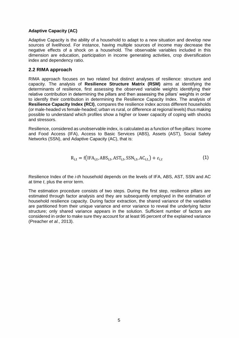
Adaptive Capacity (AC)

Adaptive Capacity is the ability of a household to adapt to a new situation and develop new sources of livelihood. For instance, having multiple sources of income may decrease the negative effects of a shock on a household. The observable variables included in this dimension are education, participation in income generating activities, crop diversification index and dependency ratio.

2.2 RIMA approach

RIMA approach focuses on two related but distinct analyses of resilience: structure and capacity. The analysis of Resilience Structure Matrix (RSM) aims at identifying the determinants of resilience, first assessing the observed variable weights identifying their relative contribution in determining the pillars and then assessing the pillars’ weights in order to identify their contribution in determining the Resilience Capacity Index. The analysis of Resilience Capacity Index (RCI), compares the resilience index across different households (or male-headed vs female-headed; urban vs rural, or difference at regional levels) thus making possible to understand which profiles show a higher or lower capacity of coping with shocks and stressors.

Resilience, considered as unobservable index, is calculated as a function of five pillars: Income and Food Access (IFA), Access to Basic Services (ABS), Assets (AST), Social Safety Networks (SSN), and Adaptive Capacity (AC), that is:

Ri,t = f(IFAi,t, ABSi,t, ASTi,t, SSNi,t, ACi,t,) + 𝜀𝑖,𝑡 (1)

Resilience Index of the i-th household depends on the levels of IFA, ABS, AST, SSN and AC at time t, plus the error term.

The estimation procedure consists of two steps. During the first step, resilience pillars are estimated through factor analysis and they are subsequently employed in the estimation of household resilience capacity. During factor extraction, the shared variance of the variables are partitioned from their unique variance and error variance to reveal the underlying factor structure; only shared variance appears in the solution. Sufficient number of factors are considered in order to make sure they account for at least 95 percent of the explained variance (Preacher et al., 2013).

6

Figure 2: Analysis of resilience structure according to RIMA

Despite the large number of latent variable models, RIMA adopts Structural Equation Model (SEM), which includes correlation between residual errors and a number of formal statistical tests and fit indices.

Three are the main advantages of using SEM (Acock, 2013) (Weunsch, 2012). The first one is that it is possible to identify direct and indirect effects. Direct effects refer to the direct relation between the dependent variable (the latent one) and the independent variables related to it. The indirect effect takes place when one variable has an impact on another variable through a third dependent or independent variable. An indirect effect indicates, for example, that the age of household heads could have an indirect effect on Resilience Capacity Index. The second advantage of SEM is the possibility to have multiple indicators explaining the latent variable. This means that it is possible to evaluate the effect of single indicators on the dependent variable, holding other indicators. The third advantage is the measurement error inclusion in the model. That is the main difference with path analysis. Path analysis includes error term in the prediction, but unfortunately does not control for measurement error during the process. SEM analysis, in accounting for measurement errors, provides a better understanding of how good the model predicts the actual outcome, minimizing the discrepancy between the covariance matrix of the observed variables, and the theoretical covariance matrix predicted by the model structure (Bollen, 1989) (Bollen et al., 2007).

Although this method requires a greater computational effort than factor analysis, it allows for model calibration until the satisfactory level of goodness-of-fitting is achieved.

3. Data

The data used for the model estimation comes from Uganda National Panel Survey (UNPS), which is part of the World Bank’s Living Standard Measurement Studies - Integrated Survey on Agriculture (LSMS-ISA). The original sample (wave I) was approximately composed of 3,200 households including a randomly-selected share of split-off households formed after the 2005/2006 Uganda National Household Survey (UNHS). The UNPS is representative at the

7

national, urban/rural and main regional levels (north, east, west and central regions). The initial sample was visited for two consecutive years (2009/2010 and 2010/2011). The number of original households successfully interviewed during the last round of survey is 2,239 (UBoS, 2013).

Attrition analysis has been run to assess whether there were any statistically significant difference between the number of original households successfully interviewed over three years of time with or without the split-off households; in particular a regression analysis revealed that no significant difference existed and, as a consequence, a decision was taken to do not follow the split-offs and focus on the original sample.

The original surveys included comprehensive information on household socioeconomic status, including detailed modules for expenditures and economic activities.

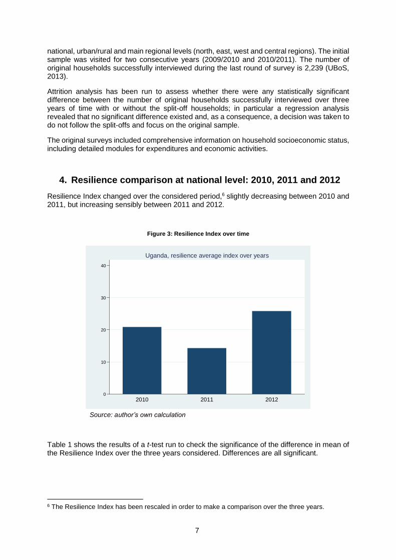
4. Resilience comparison at national level: 2010, 2011 and 2012

Resilience Index changed over the considered period,6 slightly decreasing between 2010 and 2011, but increasing sensibly between 2011 and 2012.

Figure 3: Resilience Index over time

Source: author’s own calculation

Table 1 shows the results of a t-test run to check the significance of the difference in mean of the Resilience Index over the three years considered. Differences are all significant.

6 The Resilience Index has been rescaled in order to make a comparison over the three years.

0

10

20

30

40

Resca

led In

de

x

2010 2011 2012

Uganda, resilience average index over years

8

Table 1: T-test results

Variable

2009-2010 (1)

2010-2011 (2)

2011-2012 (3)

Difference

Resilience index

20.84 14.26 6.57***

20.84 25.81 -4.96***

14.26 25.81 -11.54***

***: significative at 99% **: significative at 95% *: significative at 90%

Looking at the RSM, it is possible to draw out which pillars played the main role in building RCI.

Figure 4: Resilience structure comparison over years


IFA, together with AC, are consistently the most relevant dimension in all the three years, accounting both for more than 30 percent of importance. ABS and SSN are the only pillars that significantly change their relevance over time.

ABS increases from year 1 to year 2 but then decreases from year 2 to year 3. From Table 4 in the annexes came out that, keeping distance variables fixed, what plays the differences in the dynamics of the pillar is the infrastructure index. The fact that in year 3 ABS is even lower that in year 1 could suggests that there has been a deterioration in both infrastructure and roads conditions.

The relevance of AST is the same along the three years.

Looking at the relationship of resilience and self-reported shocks in each year, weather shocks seem to be the most important ones, although there is great mobility.

02

04

06

08

01

00

2010 2011 2012

National Level

Share of components

IFA ABS AST SSN AC

9

Figure 5: Shocks role at national level in percentage


From year 1 to year 2, weather shocks decrease their importance, together with the shocks related to the death of household members. Crop shocks, conflicts and fire significantly increase their importance. From year 2 to year 3, weather shocks continue to decrease; crop shocks also registered a decrease. Conflicts remain almost the same. Fire shocks, death of household member and livestock increase. From Figure 4 came out that crop shocks and conflicts seems to be the most important shocks causing the decrease of Resilience Index from year 1 to year 2. In fact, from year 2 to year 3 crop shocks decrease while conflicts remain almost the same.

In order to explore the most relevant livelihood strategies resilience classes have been created based on the terciles of resilience capacity distribution. The combination of the three terciles (less resilient; average resilient; more resilient) over a three-year time creates nine classes (see Table 3). Only four classes have been reported in Table 2: households who have been constantly less resilient over the three rounds; those who have been at least once at the top-resilience level; those who have been at least twice; and those who have been constantly most resilient over the three rounds.

Table 2: Income specialization among resilience categories

Less resilient all

times

Resilient once

Resilient twice

Most resilient all

times

Share of crop income in tot Inc. 51.65% 43.22% 27.68% 11.46%

Share of livestock income in tot Inc. 12.60% 13.18% 9.88% 4.21%

Share of ag. Wage in tot Inc. 10.07% 4.20% 3.08% 1.15%

Share of non ag. Wage in tot Inc. 4.98% 8.98% 16.61% 22.91%

Share of self-employment in tot Inc. 13.85% 19.04% 27.10% 35.12%

Share of transfer in tot Inc. 6.32% 8.12% 7.72% 11.62%

02

04

06

08

01

00

2010 2011 2012

National Level

Self Reported Shocks

livestock crop conflict death fire weather

10

Share of other source of Inc. 0.42% 2.30% 4.07% 8.97%

hh specialized in crop 58.90% 47.51% 29.56% 12.21%

hh specialized in livestock 14.38% 6.36% 6.35% 2.91%

hh specialized in agr wage 8.22% 1.99% 3.59% 0.87%

hh specialized in nonag wage 4.45% 11.93% 21.82% 32.85%

hh specialized in self-employment 13.36% 19.48% 30.39% 47.97%

hh specialized in transfers 4.11% 7.16% 7.46% 12.21%

hh specialized in other 0.34% 1.19% 3.87% 9.88%

Dependency ratio 2.09 1.29 0.94 0.73

hh perc of diversification 52.96% 54.5% 49.86% 40.26%

Households in the least resilience status are those with the highest crop income share, of those being most resilient in the three years the share of self-employment is the highest, considering that more than 35.12 percent of them are specialized in this activity.

There are significant differences among groups. The most resilient households have self-employment as a major source of income, followed by the non-agricultural wage. They show also a relatively low dependency ratio with respect to those households who have always been the least resilient (0.73 against 2.09). Also they are more specialized in self-employment, and the percentage of diversification is the lowest among the others. Those who have been resilient once in three year, show also a higher share or crop together with a relative low self-employment share.

Given the presence of huge regional inequality, attention has also been given to the Northern region, where the majority of poor households are concentrated.

Next figure depicts the Resilience Index average score over region in the three years considered.

Figure 6: Resilience Index Capacity over years per region


01

02

03

04

0

Ave

rag

e R

esili

en

ce In

de

x

2010 2011 2012

Cen

tral w

ith K

ampa

la

Eas

tern

Nor

ther

n

Wes

tern

Cen

tral w

ith K

ampa

la

Eas

tern

Nor

ther

n

Wes

tern

Cen

tral w

ith K

ampa

la

Eas

tern

Nor

ther

n

Wes

tern

Resilience Index over year/region

11

The northern region is the one with the lowest Resilience Index in all the three years, on the contrary Kampala region is the one with the highest. Generally there is an overall decrease from year 1 to year 2 and an overall increase from year 2 to year 3.

Figure 7: Share of component - Regional level over years


A quite intense regional variation seems to exist in Uganda; it is therefore interesting to establish the inner causes of such variability.

One approach is to look at the main determinants of changes into resilience capacity. Resilience analysis may offer limited possibility of doing causal inference.7 This is mainly due to the composite nature of the Resilience Index; the largest part of the (possible) determinants of loss/gain of resilience are already employed in the estimation procedure. As a consequence, a quite limited number of socio-economic variables may be employed in establishing causal relation with variation in resilience capacity. Probabilistic models have been employed in the next parts of this paper to explore the main determinants of intra-classes movements.

Another interesting approach is to look at the negative determinants of loss in resilience; in other words, it is interesting to explore the role of shocks into household resilience capacity. Both covariate and idiosyncratic shocks have been remained excluded from the estimation model, so that they can be employed as exogenous variables. Next chapter will focus on this topic.

7 Although there do exist dynamic latent variable models that could be adopted (see Ceriani and Giglirano, 2011).

02

04

06

08

01

00

2010 2011 2012

Kam

pala

Cen

tral

Eas

tern

Nor

ther

n

Wes

tern

Kam

pala

Cen

tral

Eas

tern

Nor

ther

n

Wes

tern

Kam

pala

Cen

tral

Eas

tern

Nor

ther

n

Wes

tern

Share of component at regional level over years

IFA ABS AST SSN AC

12

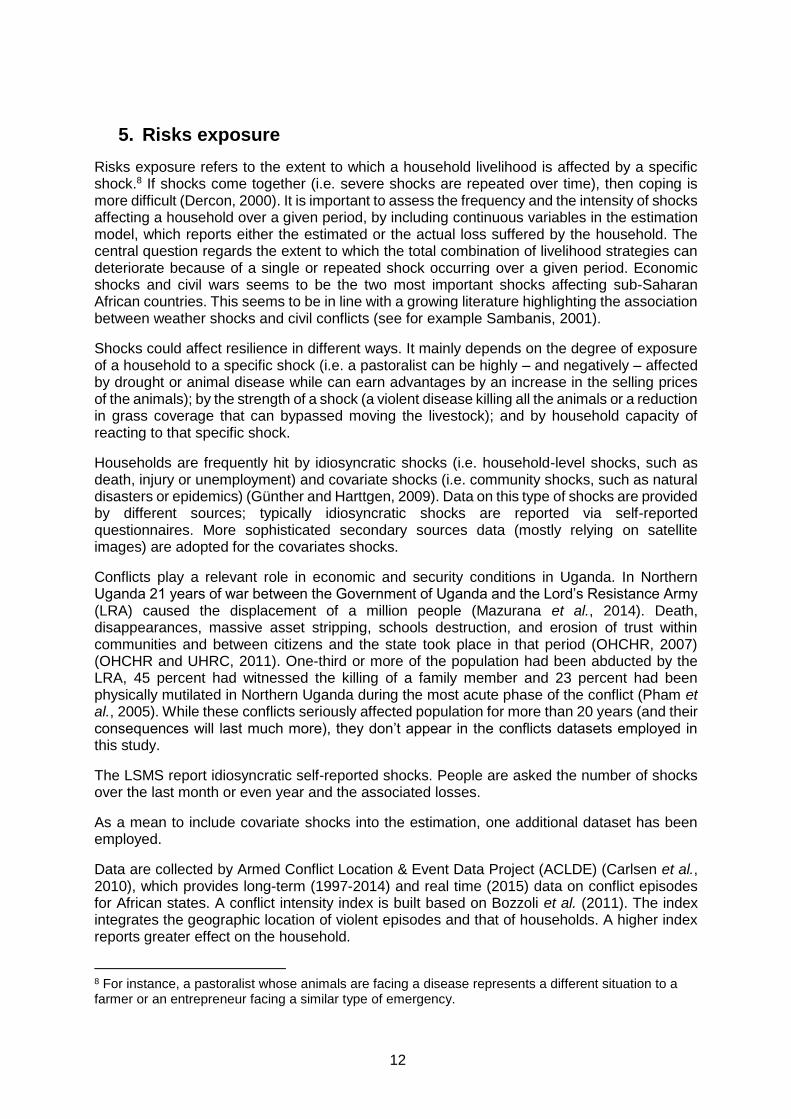
5. Risks exposure

Risks exposure refers to the extent to which a household livelihood is affected by a specific shock.8 If shocks come together (i.e. severe shocks are repeated over time), then coping is more difficult (Dercon, 2000). It is important to assess the frequency and the intensity of shocks affecting a household over a given period, by including continuous variables in the estimation model, which reports either the estimated or the actual loss suffered by the household. The central question regards the extent to which the total combination of livelihood strategies can deteriorate because of a single or repeated shock occurring over a given period. Economic shocks and civil wars seems to be the two most important shocks affecting sub-Saharan African countries. This seems to be in line with a growing literature highlighting the association between weather shocks and civil conflicts (see for example Sambanis, 2001).

Shocks could affect resilience in different ways. It mainly depends on the degree of exposure of a household to a specific shock (i.e. a pastoralist can be highly – and negatively – affected by drought or animal disease while can earn advantages by an increase in the selling prices of the animals); by the strength of a shock (a violent disease killing all the animals or a reduction in grass coverage that can bypassed moving the livestock); and by household capacity of reacting to that specific shock.

Households are frequently hit by idiosyncratic shocks (i.e. household-level shocks, such as death, injury or unemployment) and covariate shocks (i.e. community shocks, such as natural disasters or epidemics) (Günther and Harttgen, 2009). Data on this type of shocks are provided by different sources; typically idiosyncratic shocks are reported via self-reported questionnaires. More sophisticated secondary sources data (mostly relying on satellite images) are adopted for the covariates shocks.

Conflicts play a relevant role in economic and security conditions in Uganda. In Northern Uganda 21 years of war between the Government of Uganda and the Lord’s Resistance Army (LRA) caused the displacement of a million people (Mazurana et al., 2014). Death, disappearances, massive asset stripping, schools destruction, and erosion of trust within communities and between citizens and the state took place in that period (OHCHR, 2007) (OHCHR and UHRC, 2011). One-third or more of the population had been abducted by the LRA, 45 percent had witnessed the killing of a family member and 23 percent had been physically mutilated in Northern Uganda during the most acute phase of the conflict (Pham et al., 2005). While these conflicts seriously affected population for more than 20 years (and their consequences will last much more), they don’t appear in the conflicts datasets employed in this study.

The LSMS report idiosyncratic self-reported shocks. People are asked the number of shocks over the last month or even year and the associated losses.

As a mean to include covariate shocks into the estimation, one additional dataset has been employed.

Data are collected by Armed Conflict Location & Event Data Project (ACLDE) (Carlsen et al., 2010), which provides long-term (1997-2014) and real time (2015) data on conflict episodes for African states. A conflict intensity index is built based on Bozzoli et al. (2011). The index integrates the geographic location of violent episodes and that of households. A higher index reports greater effect on the household.

8 For instance, a pastoralist whose animals are facing a disease represents a different situation to a farmer or an entrepreneur facing a similar type of emergency.

13

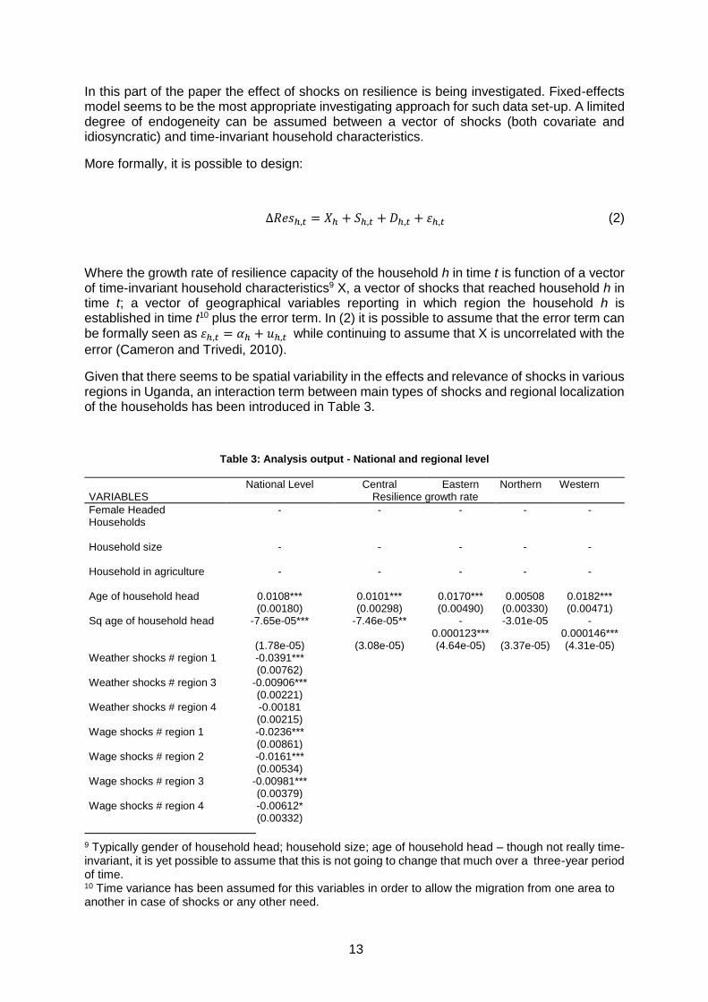
In this part of the paper the effect of shocks on resilience is being investigated. Fixed-effects model seems to be the most appropriate investigating approach for such data set-up. A limited degree of endogeneity can be assumed between a vector of shocks (both covariate and idiosyncratic) and time-invariant household characteristics.

More formally, it is possible to design:

∆𝑅𝑒𝑠ℎ,𝑡 = 𝑋ℎ + 𝑆ℎ,𝑡 + 𝐷ℎ,𝑡 + 𝜀ℎ,𝑡 (2)

Where the growth rate of resilience capacity of the household h in time t is function of a vector of time-invariant household characteristics9 X, a vector of shocks that reached household h in time t; a vector of geographical variables reporting in which region the household h is established in time t10 plus the error term. In (2) it is possible to assume that the error term can be formally seen as 𝜀ℎ,𝑡 = 𝛼ℎ + 𝑢ℎ,𝑡 while continuing to assume that X is uncorrelated with the

error (Cameron and Trivedi, 2010).

Given that there seems to be spatial variability in the effects and relevance of shocks in various regions in Uganda, an interaction term between main types of shocks and regional localization of the households has been introduced in Table 3.

Table 3: Analysis output - National and regional level

National Level Central Eastern Northern Western VARIABLES Resilience growth rate

Female Headed Households

- - - - -

Household size - - - - - Household in agriculture - - - - - Age of household head 0.0108*** 0.0101*** 0.0170*** 0.00508 0.0182*** (0.00180) (0.00298) (0.00490) (0.00330) (0.00471) Sq age of household head -7.65e-05*** -7.46e-05** -

0.000123*** -3.01e-05 -

0.000146*** (1.78e-05) (3.08e-05) (4.64e-05) (3.37e-05) (4.31e-05) Weather shocks # region 1 -0.0391*** (0.00762) Weather shocks # region 3 -0.00906*** (0.00221) Weather shocks # region 4 -0.00181 (0.00215) Wage shocks # region 1 -0.0236*** (0.00861) Wage shocks # region 2 -0.0161*** (0.00534) Wage shocks # region 3 -0.00981*** (0.00379) Wage shocks # region 4 -0.00612* (0.00332)

9 Typically gender of household head; household size; age of household head – though not really time-invariant, it is yet possible to assume that this is not going to change that much over a three-year period of time. 10 Time variance has been assumed for this variables in order to allow the migration from one area to another in case of shocks or any other need.

14

Crop shocks 0.00351 -0.00579 -0.00235 0.0142 0.0283 (0.0108) (0.0233) (0.0135) (0.0364) (0.0273) Conflict intensity -0.000124 4.97e-05 -0.0269*** -

0.00336** 0.0122***

(0.000220) (0.000273) (0.00203) (0.00144) (0.00244) Conflict shocks # region 1 0.00256 (0.0276) Conflict shocks # region 2 0.0168 (0.0151) Conflict shocks # region 3 0.00559 (0.00770) Conflict shocks # region 4 0.0158* (0.00874) Input/output shocks 0.0265*** 0.0176 0.0188* 0.0547** -0.0179 (0.00938) (0.0258) (0.00981) (0.0259) (0.0433) Livestock disease -0.0144 -0.0190 -0.00648 -0.000704 0.0887 (0.0126) (0.0254) (0.0154) (0.0268) (0.127) Length of shocks -0.000304 -0.00371* 0.00429** -0.00112 0.00135 (0.000910) (0.00215) (0.00178) (0.00139) (0.00226) No food -0.0305*** -0.0500*** -0.0220*** -0.0159*** -0.0316*** (0.00417) (0.0107) (0.00680) (0.00612) (0.00944) Other shocks -0.0164 -0.0126 -0.0260 -0.00339 -0.0186 (0.0103) (0.0243) (0.0290) (0.0152) (0.0173) Eastern region -0.139 (0.0950) Northern region - Western region - Weather shocks -0.0209* -0.00744 -0.0293*** -0.0102 (0.0112) (0.00766) (0.00644) (0.0104) Wage shocks -0.0153 -0.0332*** -0.0302*** -0.0247* (0.0109) (0.00901) (0.00984) (0.0142) Conflict shocks 0.00108 0.0320 0.0203 0.0635* (0.0336) (0.0253) (0.0194) (0.0335) Constant -0.267*** -0.263*** -0.464*** -0.136* -0.474*** (0.0493) (0.0713) (0.125) (0.0775) (0.125) Observations 6,719 1,967 1,611 1,728 1,413 R-squared 0.060 0.068 0.211 0.084 0.076 Number of hh 2,240 657 538 576 471


Model (1) of table 3 presents the results with the entire datasets and includes interaction terms between weather, wage and self-reported conflict shocks with regional localization. Model (2) to (4) disaggregate results for regions (i.e.: central, eastern, northern and western regions). Conflicts, wage- and weather-related shocks negatively affect resilience. Interestingly the variable “conflict intensity” (the one abovementioned for intensity of conflicts) does not have any relevant effect at national level; however it does when looking at the data disaggregated for region. Even in this case, therefore, there seems to be a lot of spatial variability due to regional specificity (see interaction terms); this correlates with well-known instable situation in areas such as the northern regions particularly exposed to disorders.

In general, it seems like regional differences largely explain the effects of shocks on resilience and on resilience growth. Uganda is in fact a quite heterogeneous country with many differences from central and Kampala areas as compared with other (especially northern) regions. This will inform the analyses presented in the next chapters.

Results suggest other interesting findings. On average, older heads of household are paired with greater resilience capacity; however, when they are too old (indicated by the squared age of household head) resilience capacity slightly reduces (Table 3). It came out that older heads

15

of household have lower adaptive capacity and less ability to contribute to family income generating activities.

6. Dynamic analysis

Dynamic framework is necessary to assess how the resilience capacity of i-th household changes over time together with the main drivers of change.

There are different ways to measure variations over time; in this paper transition matrices are employed to carry out an inter-temporal analysis of resilience capacity. Transition matrices have been largely applied in poverty analysis, in order to distinguishing households that are poor occasionally from those that are poor all the time.

The use of transition matrices might present problems since there are measurement errors in the outcome variable (e.g. household poverty, income or resilience). In order to avoid these problems households are classified into resilience capacity classes (given by the terciles of Resilience Index distribution). However, this does not allow getting full information about the distance between two different households. Furthermore, it is not possible to compare transition matrices across different contexts (e.g. countries) because the Resilience Index is context-specific and the periods spanned by panel surveys may be different (Shepherd and Brunt, 2013).

Resilience transitional matrices show the share of households who remain, move out or in a given resilience class (i.e. RCI terciles: high, medium and low resilience) across different years (Table 4).

Table 4: Mobility among resilience terciles - National and regional level

Percentage Frequency

National

2011 2011

2010

Least resilient

Less resilient

Most resilient

2010 Least

resilient Less

resilient Most

resilient Row total

Least resilient 66 28 6 Least resilient 486 202 45 733

a) Less resilient 29 47 24 Less resilient 220 365 184 769

Most resilient 7 25 68 Most resilient 54 182 502 738

Column total 760 749 731 2240

2012 2012

2011

Least resilient

Less resilient

Most resilient

2011 Least

resilient Less

resilient Most

resilient Row total


b) Less resilient 26 51 23 Less resilient 194 382 173 749


Column total 739 767 734 2240

2012 2012

16

2010 Least

resilient Less

resilient Most

resilient 2010

Least resilient

Less resilient

Most resilient

Row total


c) Less resilient 25 52 22 Less resilient 196 403 170 769


Column total 739 767 734 2240

Central with Kampala

2012 2012

Least resilient

Less resilient

Most resilient

2010 Least

resilient Less

resilient Most

resilient Row total




Column total 96 186 367 649

2012 2012

Least resilient

Less resilient

Most resilient

2010 Least

resilient Less

resilient Most

resilient Row total

b) Least resilient 49 39 13 Least resilient 47 37 12 96

Less resilient 24 42 34 Less resilient 44 79 63 186



2012 2012

Least resilient

Less resilient

Most resilient

2010 Least

resilient Less

resilient Most

resilient Row total





Eastern

2011 2011

2010

Least resilient

Less resilient

Most resilient

2010 Least

resilient Less

resilient Most

resilient Row total




Column total 209 202 125 536

2012 2012

2011

Least resilient

Less resilient

Most resilient

2011 Least

resilient Less

resilient Most

resilient Row total


17



Column total 197 207 132 536

2012 2012

2010

Least resilient

Less resilient

Most resilient

2010 Least

resilient Less

resilient Most

resilient Row total




Column total 197 207 132 536

Northern

2011 2011

2010

Least Resilient

Less Resilient

Most Resilient

2010 Least

resilient Less

resilient Most

resilient Row total





2012 2012

2011 Least

resilient Less

resilient Most

resilient 2011

Least resilient

Less resilient

Most resilient

Row total




Column total 289 187 100 576

2012 2012

2010 Least

resilient Less

resilient Most

resilient 2010

Least resilient

Less resilient

Most resilient

Row total




Column total 289 187 100 576

Western

2011 2011

2010 Least

resilient Less

resilient Most

resilient 2010

Least resilient

Less resilient

Most resilient

Row total



18


Column total 151 171 149 471

2012 2012

2011 Least

resilient Less

resilient Most

resilient 2011

Least resilient

Less resilient

Most resilient

Row total




Column total 154 190 127 471

2012 2012

2010

Least resilient

Less resilient

Most resilient

2010 Least

resilient Less

resilient Most

resilient Row total




Column total 154 190 127 471

Six percent of the households that were in the least resilient status in 2010 become most resilient in 2011, 28 percent migrated to the medium terciles and 66 percent remained in the same class. Considering the most resilient households in 2010, 7 percent became the least resilient in 2011, 25 percent moved to the medium resilience class and 68 percent remained in the same class (Table 4a).

Those who remain in the least resilient status are the consistently less resilient. The mobility across terciles is not so high considering the extreme categories; in fact in all the three sub-tables almost the 50 percent of the households remain in the same least resilience position. Same thing happen for those who have been always the most resilient households: more than 60 percent of them, on average, remain in the same terciles (most resilient all the time).

69percent of the least resilient households in 2010 remained in the same status in 2012 (the well-known poverty trap), 28 percent improved their situation moving in the medium resilient class, and 4 percent became the most resilient in 2012 (2010-2012, Table 4c). Interestingly 25 percent of the middle-resilient households became least resilient; while 5 percent of the most resilient migrated into the least resilient status. However, provided the spatial differences emerged above, a further disaggregation has been applied and interesting results emerge. Table 3 presents transition matrices for the 4 macro-regions: central (including Kampala), eastern, northern and western.

Northern region presents the highest percentage of persistence in the lowest class of resilience capacity (75 percent, 76 percent and 78 percent in Tables 4a, b and c of northern region). This indicates a lower capacity of transitioning from bottom to higher level. Furthermore northern region reports the highest share of households sliding from middle- to bottom-class of resilience capacity (Table 3c): 35 percent of households in northern region migrated from less to least resilient status between 2010 and 2012 as compared with 26 percent for eastern; 21 percent western and 19 percent for central region. Once again this finding highlights how relevant spatial differences exist within Uganda.

19

Based on the reported tables, it is therefore interesting to establish causal evidence of determinants of persistence or migration within resilience capacity classes, with particular reference to spatial differences. Many studies have recently used the multinomial logit model to analyse the factors affecting the probability that a household moves from a certain status to another (for instance across different income classes). One of the main advantages of such an approach is its simple specification (Grosh and Glewwe, 1995) (Grootaert and Kanbur, 1995).

Multinomial logit models are adopted for studying a dependent categorical variable that can fall into one of several mutually exclusive categories. In this case three multinomial logit models were run for the three years of study with three possible categories in each year, corresponding to the three aforementioned classes of resilience capacity. Table 5 reports the estimates of multinomial logit, considering household being always the least resilient as the base category and presenting findings for three possible scenarios: (2) most resilient at least once; (3) most resilient twice; (4) persistently most resilient.

Table 5: Mlogit results

VARIABLES Most resilient

once

Most resilient twice

Always most resilient

Female household head

-0.503** -0.765*** -0.529**

(0.204) (0.235) (0.262) Household size -0.225*** -0.365*** -0.345*** (0.0342) (0.0403) (0.0435) Average yy of education

0.601*** 0.768*** 1.007***

(0.0663) (0.0707) (0.0744) Chronic poverty -2.473*** -4.465*** -17.48 (0.415) (1.130) (853.4) Log of pc exp (second diff)

-0.238** -0.161 -0.584***

(0.117) (0.131) (0.149) Log of precipitation -1.578*** -2.242*** -3.173*** (0.583) (0.672) (0.840) Average share of crop income

-1.229*** -2.886*** -4.886***

(0.360) (0.416) (0.507) Average share of self-employment

0.412 0.516 0.618

(0.446) (0.474) (0.497) Log of Wet index -0.0588 0.236 -0.344 (0.522) (0.619) (0.782) Distance from populated centre (+200000)

-0.00984** -0.0143** -0.0461***

(0.00494) (0.00592) (0.00801) Northern -1.545*** -2.141*** -3.586*** (0.211) (0.258) (0.363) Constant 13.51** 16.71** 26.84*** (5.917) (6.950) (8.937) Observations 1,484 1,484 1,484


20

The relative probability of being most resilient at least once in the three years (category two), rather than being always the least resilient (base category) is negative for female household heads than male ones. The relative probability of being even most resilient in two years (category three) increases negatively. Education has the biggest (and positive) impact on the relative probabilities of being resilient once, twice or always rather than being always the least resilient; for instance the higher the level of household’s education, the higher the relative probability of being not in the base category is. This is in line with findings from other studies in Uganda (see Mazurana et al., 2014) highlighting the relevance of education to pull people out of poverty.

The relative probability of being always most resilient (all the three years) rather than being always the least resilience is lower if the share of crop income of income increase over time. One problem when analysing transitions is that the relative probability of making the second transition (from being the least resilient to being resilient at least once) depends on whether or not the households have previously made the first transition (that is being least resilient all the time); that is the second transition always represents a selected sample. This is known as the “independence of invariant alternatives” as a consequence of the implied assumption that there is “no correlation between the error terms”. The multinomial model is therefore not the perfect set for analysing transitions as it takes initial least resilient status as exogenous, thus requiring that persistence in this status is entirely due to observable explanatory variables. Correlation across time between unobservable will therefore create a sample selection bias due to the conditioning on the initial.

One of the most adopted solution to avoid problems related to multinomial logit and independence of invariant alternatives is to consider the factors that are associated with whether a household is the least resilient or the most resilient starting with factors associated with changes (or not) in the household’s resilience status between 2010 and 2012. The analysis is focused on two conditional probabilities of being in a status given another status: (1) the probability of being the least resilient in year 3 (i.e. 2012) conditional to being the least resilient in year 1 (i.e. 2010); and (2) the probability of being the least resilient in year 3 conditional to not being the least resilient in year 1. Covariate and idiosyncratic shocks are reported; as above, the formers are self-reported shocks, while a conflict intensity variable represent covariate shocks. Results are further disaggregated at regional level, standing the spatial differentiations presented above.

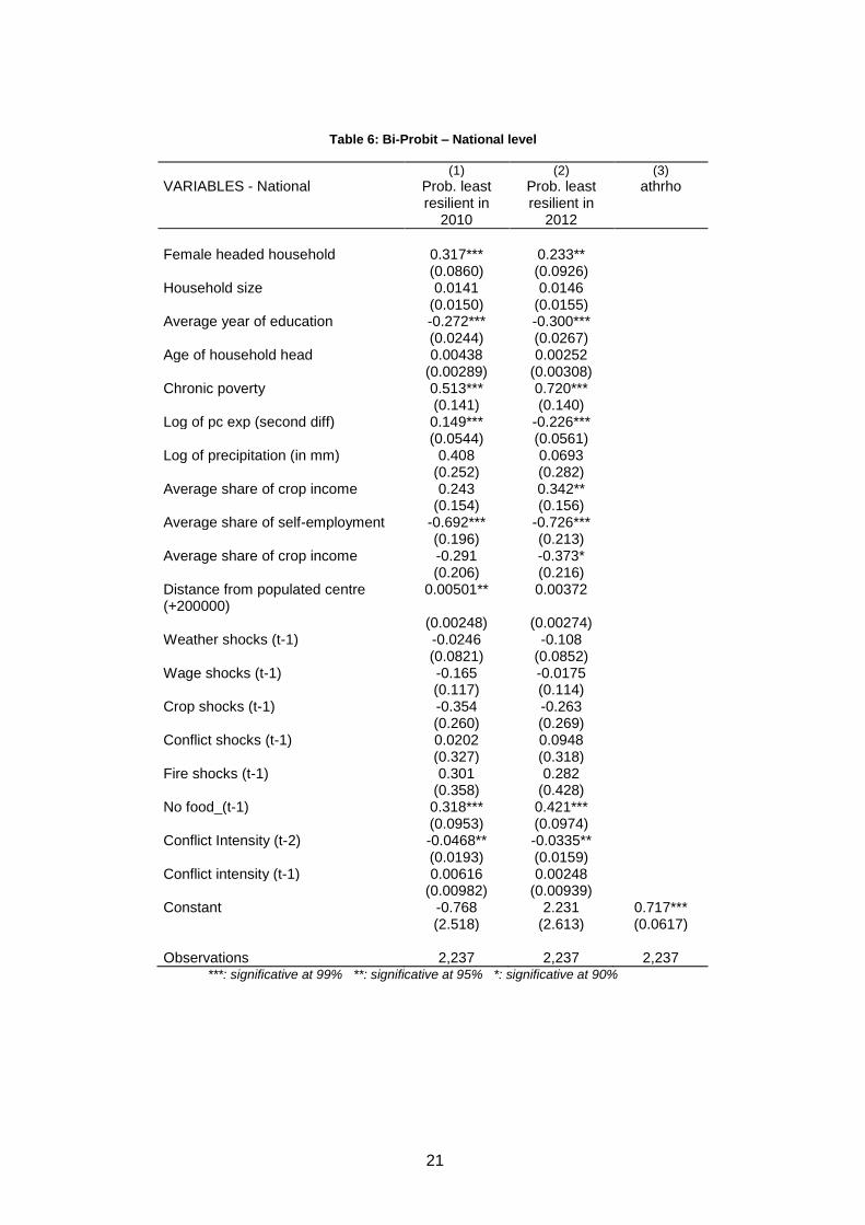
21

Table 6: Bi-Probit – National level

(1) (2) (3)

VARIABLES - National Prob. least resilient in

2010

Prob. least resilient in

2012

athrho

Female headed household 0.317*** 0.233** (0.0860) (0.0926) Household size 0.0141 0.0146 (0.0150) (0.0155) Average year of education -0.272*** -0.300*** (0.0244) (0.0267) Age of household head 0.00438 0.00252 (0.00289) (0.00308) Chronic poverty 0.513*** 0.720*** (0.141) (0.140) Log of pc exp (second diff) 0.149*** -0.226*** (0.0544) (0.0561) Log of precipitation (in mm) 0.408 0.0693 (0.252) (0.282) Average share of crop income 0.243 0.342** (0.154) (0.156) Average share of self-employment -0.692*** -0.726*** (0.196) (0.213) Average share of crop income -0.291 -0.373* (0.206) (0.216) Distance from populated centre (+200000)

0.00501** 0.00372

(0.00248) (0.00274) Weather shocks (t-1) -0.0246 -0.108 (0.0821) (0.0852) Wage shocks (t-1) -0.165 -0.0175 (0.117) (0.114) Crop shocks (t-1) -0.354 -0.263 (0.260) (0.269) Conflict shocks (t-1) 0.0202 0.0948 (0.327) (0.318) Fire shocks (t-1) 0.301 0.282 (0.358) (0.428) No food_(t-1) 0.318*** 0.421*** (0.0953) (0.0974) Conflict Intensity (t-2) -0.0468** -0.0335** (0.0193) (0.0159) Conflict intensity (t-1) 0.00616 0.00248 (0.00982) (0.00939) Constant -0.768 2.231 0.717*** (2.518) (2.613) (0.0617) Observations 2,237 2,237 2,237


22

Table 7: Bi-Probit – Central Region (incl. Kampala)

(1) (2) (3) VARIABLES – Central Prob. least

resilient in 2010


2012

athrho

Female headed household 0.342* 0.0353 (0.183) (0.192) Household size 0.0231 -0.0265 (0.0248) (0.0305) Average year of education -0.227*** -0.201*** (0.0483) (0.0556) Chronic poverty 0.462 1.176** (0.522) (0.529) Log of pc exp (second diff) 0.137 -0.387*** (0.131) (0.111) Log of precipitation (in mm) -0.552 0.292 (0.697) (0.741) Average share of crop income 0.466 0.884** (0.336) (0.358) Average share of self-employment -0.871** -0.367 (0.367) (0.374) Average share of crop income 1.265 1.922 (1.814) (2.121) Distance from populated centre (+200000)

-0.00588 0.00371

(0.00674) (0.00716) Weather shocks (t-1) 0.247 0.0556 (0.181) (0.216) Wage shocks (t-1) -0.317 -0.306 (0.272) (0.234) Crop shocks (t-1) -0.108 0.747** (0.495) (0.381) Conflict shocks (t-1) -6.771*** -6.432*** (0.408) (0.344) Fire shocks (t-1) -5.425*** -5.200*** (0.303) (0.369) No food_(t-1) 0.235 0.511* (0.235) (0.300) Conflict Intensity (t-2) -0.0258 -0.0405** (0.0157) (0.0185) Conflict intensity (t-1) 9.61e-05 0.0155** (0.00783) (0.00743) Constant -5.082 -16.23 0.521*** (16.18) (19.16) (0.141) Observations 655 655 655


23

Table 8: Bi-Probit – Eastern regions

(1) (2) (3) VARIABLES - Eastern Prob. least

resilient in 2010


2012

athrho

Female headed household 0.640*** 0.409** (0.173) (0.182) Household size -0.0139 -0.0189 (0.0293) (0.0263) Average year of education -0.252*** -0.400*** (0.0449) (0.0517) Chronic poverty 0.389 0.813*** (0.253) (0.258) Log of pc exp (second diff) 0.304*** -0.0744 (0.105) (0.104) Log of precipitation (in mm) -0.486 -0.457 (1.312) (1.400) Average share of crop income -0.0314 0.0554 (0.259) (0.262) Average share of self-employment -0.669** -0.549 (0.334) (0.345) Average share of crop income -0.0611 -0.152 (0.902) (0.901) Distance from populated centre (+200000)

0.00310 -0.00114

(0.00629) (0.00683) Weather shocks (t-1) -0.156 -0.0184 (0.159) (0.160) Wage shocks (t-1) -0.0476 -0.0107 (0.196) (0.201) Crop shocks (t-1) -0.0775 -0.379 (0.411) (0.412) Conflict shocks (t-1) -0.731 -11.41*** (0.788) (1.086) Fire shocks (t-1) -6.417*** -7.050*** (0.248) (0.256) No food_(t-1) 0.232 0.358** (0.179) (0.174) Conflict Intensity (t-2) 0.0323 -0.188** (0.0785) (0.0865) Conflict intensity (t-1) -0.0355 0.0718 (0.0529) (0.0557) Constant 4.549 5.434 0.855*** (6.195) (7.062) (0.115) Observations 535 535 535


24

Table 9: Bi-Probit – Northern regions

(1) (2) (3) VARIABLES - Northern Prob. least

resilient in 2010


2012

athrho

Female headed household 0.113 -0.0765 (0.171) (0.172) Household size 0.00595 -0.00458 (0.0298) (0.0314) Average year of education -0.345*** -0.369*** (0.0558) (0.0495) Chronic poverty 0.379* 0.731*** (0.211) (0.218) Log of pc exp (second diff) 0.135 -0.183 (0.106) (0.117) Log of precipitation (in mm) 0.0517 0.133 (0.631) (0.593) Average share of crop income 0.505 0.560 (0.370) (0.386) Average share of self-employment 0.000370 -0.477 (0.338) (0.354) Average share of crop income -0.611* -0.148 (0.359) (0.374) Distance from populated centre (+200000)

0.00375 0.00428

(0.00381) (0.00401) Weather shocks (t-1) -0.242* -0.226 (0.129) (0.140) Wage shocks (t-1) 0.278 0.234 (0.264) (0.260) Crop shocks (t-1) 0.730 0.589 (0.742) (0.800) Conflict shocks (t-1) 1.560*** 11.93*** (0.604) (1.036) Fire shocks (t-1) 1.819*** 1.707*** (0.486) (0.530) No food_(t-1) 0.216 0.230 (0.166) (0.163) Conflict Intensity (t-2) -0.122** -0.0478 (0.0505) (0.0460) Conflict intensity (t-1) 0.0221 0.0809 (0.0470) (0.0547) Constant 4.615 0.812 0.643*** (4.662) (4.642) (0.106) Observations 576 576 576


25

Table 10: Bi-Probit – Western regions

(1) (2) (3) VARIABLES - Western Prob. least

resilient in 2010


2012

athrho

0.305* 0.394** Female headed household (0.174) (0.173) 0.0479 0.0682** Household size (0.0311) (0.0329) -0.322*** -0.269*** Average year of education (0.0540) (0.0446) 0.887*** 0.549** Chronic poverty (0.322) (0.273) 0.0906 -0.261** Log of pc exp (second diff) (0.103) (0.104) 0.241 -0.940 Log of precipitation (in mm) (0.658) (0.666) 0.204 0.141 Average share of crop income (0.311) (0.309) -1.098* -1.651** Average share of self-employment (0.610) (0.664) -0.0548 0.0541 Average share of crop income (0.431) (0.420) 0.00543 0.00511 Distance from populated centre (+200000)

(0.00761) (0.00778)

0.119 -0.138 Weather shocks (t-1) (0.221) (0.236) -0.396 0.102 Wage shocks (t-1) (0.295) (0.239) -0.949** -0.649 Crop shocks (t-1) (0.482) (0.469) -0.0915 0.342 Conflict shocks (t-1) (0.786) (0.816) -4.853*** -4.871*** Fire shocks (t-1) (0.396) (0.359) 0.556*** 0.542** No food_(t-1) (0.214) (0.210) -0.0737 0.0939 Conflict Intensity (t-2) (0.0873) (0.106) 0.0223 -0.204** Conflict intensity (t-1) (0.0847) (0.0910) -1.199 6.137 0.821*** (5.628) (5.625) (0.126) Observations 471 471 471

Robust standard errors in parentheses. ***: significative at 99% **: significative at 95% *: significative at 90%

At national level the probabilities of remaining in the bottom-class of resilience capacity is highly influenced by the presence of a female household head; having a large share of income proceeding from crop activities; and having suffered with shocks that ultimately forced the household to stay without food for some days. Average educational level, per capita expenditure and participating a self-enterprise reduce the probability of persistence in the

26

lowest resilience capacity group. These findings depicts a situation where female-headed household more connected to farming activities and fewer educational level are more exposed to remain in difficult situation than an male-headed household which invests in education and self-enterprises.

Interestingly no evidence exists in Table 6 (analysis at national level) of the relevance of conflict on persistency in the same (lowest) class of resilience capacity. The figures however change dramatically when looking at the same models under a regional perspective (see Tables 7, 8, 9 and 10 for the analysis at regional level). Table 8, for the eastern region, shows that conflict (idiosyncratic self-reported) shocks play a major role in explaining persistency in the lowest resilience class. This finding is in line with other relevant studies in the area (see Mazurana et al., 2014 or De Luca and Verpoorten, 2015). On the contrary the conflict intensity variable does not seem to be able to capture the existence and effect of shocks in northern regions.

Table 6 reports the same model for central Region; that partially (geographically) overlap with the old Buganda. Being involved in crop activities seems to be one of the major determinants of persistency in the lowest class of resilience. This highly correlates with the traditional relevance of farming activities in the area.

7. Conclusions

Resilience is, nowadays, one of the key-words for any action or programme in development environment. A number of studies have adopted this approach; policy makers have re-tuned their actions. As a result, many attempts of measuring resilience popped-out proposing both quantitative and qualitative approaches. This paper defines resilience as “a capacity that ensures stressors and shocks do not have long-lasting adverse development consequences” (TWG-RM, 2014).

Household resilience to food insecurity is measured through the RIMA approach. This paper estimates the dynamic of resilience looking at the intertemporal resilience capacity variation and at the transition matrices; furthermore, multinomial logit and bivariate probit models are run in order to estimate what are the main drivers of resilience persistency and resilience mobility.

The main findings are that households with female head are less likely to stay or enter the most resilient tercile; household size also negatively affects the possibility of being in that tercile. Those who are involved in crop activities most likely belong to the bottom terciles. On the contrary, education and participation into self-enterprises positively affect the probability of being the most resilient in the country.11 Finally, conflicts, weather and wage shocks are relevant determinants of persistency in the lowest resilience capacity class, with a strong spatial differentiation.

This paper contributes to the literature on resilience dynamics by clarifying the determinants of migration from low to high resilience capacity. Still more has to be done, in establishing a direct causal relation between resilience capacity and its main drivers.

In particular, latent variable models reduce the possibility of inference. This affects the scope of the analysis that can be done and the consequent types of indications that can be drawn.

11 see Mazurana et al. (2014) for a similar conclusion with regard to conflict affected population in Uganda.

27

Dynamic latent variable models can be adopted in order to move the analysis on. Yet more, the introduction of regression based approaches at estimating resilience and proxy of resilience broaden the scope and possibilities of the research.

28

References

Acock, A. C. 2013. Discovering Structural Equation Modeling Using Stata. Stata Press.

Adger, W. 2006. Vulnerability. Global Environmental Change, 16: 268-281.

Alinovi, L., Mane, E. & Romano, D. 2008. Measuring household resilience to food insecurity: application to palestinian households, Agricultural Survey Methods.

Batabyal, A. A. 1998. The concept of resilience: retrospect and prospect. Environment and Development Economics, 3(2): 235-239.

Benè, C. 2013. Towards a Quantifiable Measure of Resilience. IDA Working Paper.

Bollen, K. A. 1989. Structural Equations with Latent Variables. New York. John Wiley.

Bollen, K. A., Bauer, D. J., Christ, S. L. & Edwards, M. C. 2007. An overview of structural equation models and recent elaborations. In: Recent Developments in social science statistics. New York, John Wiley, pp. 37-79.

Bozzoli, C., Bruck, T. & Muhumuza, T. 2011. Does war influence individual expenctations?. Economic letters, 113: 288-291.

Cameron, A. C. & Trivedi, K. P. 2005. Microeconometrics: Methods and Applications. New York, Cambridge University Press.

Carlsen, J., Hegre, H., Linke, A. & Raleigh, C. 2010. Introducing ACLED: an armed conflict location and event dataset. Journal of Peace Research, 47(5): 1-10.

Ceriani, L. & Gigliarano, C. 2011. An Intertemporal relative deprivation index. Society for the Study of Economic Inequtality, 124(2): 427-443.

Ciani, F. & Romano, D. 2011. A resilience-based approach to food insecurity: the impact of mitch hurricane on rural household in Nicaragua. Dipartimento di Scienze per l’Economia e l’Impresa, Università degli Studi di Firenze.

De Luca G. and Verpoorten M. 2015. Civil war, social capital and resilience in Uganda. Oxford Economic Papers. 67(3): 661-686.

Dercon, S. 2000. Income risk, coping strategies and safety nets. Background paper World Development Report 2000/2001, 17(2): 141-166.

Dercon, S. & Krishnan, P. 1998. Changes in Poverty in Rural Ethiopia 1989-1995: Measurement, Robustness Tests and Decomposition. Center for Economic Studies - Discussion papers ces9819, Katholieke Universiteit Leuven, Centrum voor Economische Studiën.

FAO. 2013. Resilience Index Measurement and Analysis model (available at www.fao.org/3/a-i4102e.pdf).

Frankenberger, T., Spangler, T., Nelson, S. & Langworthy, M. 2012. Enhancing Resilience to Food Security Shocks in Africa. FSSN Discussion Paper (available at www.fsnnetwork.org/sites/default/files/discussion_paper_usaid_dfid_wb_nov._8_2012.pdf).

Grootaert, C. & Kanbur, R. 1995. Child labour: An economic perspective. International Labour Review (Geneva), 134(2): 187-203.

Grosh, M. & Glewwe, P., 1995. A Guide to Living Standards Measurement Study Surveys and their Data Sets, Living Standards Measurement, 120, World Bank.

29

Günther, I. & Harttgen, K. 2009. Estimating Households Vulnerability to Idiosyncratic and Covariate Shocks: A Novel Method Applied in Madagascar. World Development, 37(7), 1222-1234.

Jalan, J. & Ravallion, M. 1998. Behavioral Responses to Risk in Rural China. Policy Research Working Paper 1978.

Kochar, A. 1999. Smoothing Consumption by Smoothing Income: Hours of Work Responses to Idiosyncratic Agricultural Shocks in Rural India. The Review of Economics and Statistics, 81(1): 50-61.

Levin, S. , Barrett, S. & Aniyar, S. 1998. Resilience in natural and socioeconomic systems. Environment and Development Economics, pp. 221-262.

Ligon, E. 2002. Targeting and Informal Insurance. Wider Discussion Paper, 2002/08, World Institute for Development Economics (UNU-WIDER).

Marshak, A., Opio, J. H, Gordon, R. & Atim, T. 2014. Recovery in Northern Uganda: How are people surviving post-conflicts?. Secure Livelihoods Research Consortium (SRLC) research paper (available at www.securelivelihoods.org/resources_download.aspx?resourceid=297&documentid=325).

McPeak, J. 2004. Contrasting income shocks with asset shocks: livestock sales in northern Kenya. Oxford Economic Papers, 56(2): 263-284.

Mordoch, J. 1999. Between the state and the market: can informal insurance patch the safety net?. World Bank Research Observer, 14(2): 187-207.

OHCHR (United Nations Office of the High Commissioner for Human Rights). 2007. Making peace our own: Victims’ perceptions of accountability, reconciliation and transitional justice in northern Uganda. Geneva and Kampala: OHCHR.

OHCHR and UHRC (Ugandan Human Rights Commission). 2011. The dust has not yet settled: Victims’ views on remedy and reparation in the greater north, Uganda. Kampala: OHCHR and UHRC (available at www.ohchr.org/Documents/Press/WebStories/DustHasNotYetSettled.pdf). [perche' l'hai cancellato? Hai tolto anche la citazione nel testo?]

Pan, L. 2007. Risk Pooling through Transfers in Rural Ethiopia. Tinbergen Institute Discussion Paper, 07-014/2.

Paxson, C. H. 1992. Using weather variability to estimate the response of savings to transitory income in Thailand. American Economic Review, 82(1): 15-33.

Pham, P., Vinck, P., Wierda, M., Stover, E. & di Giovanni, A. 2005. Forgotten voices: A population-based survey on attitudes about peace and justice in northern Uganda. Berkeley. Human Rights Center.

Pingali, P., Alinovi, L. & Sutton, J. 2005. Food security in complex emergencies: enhancing food system resilience. Disaster, 29(1): 5-24.

Preacher, K. J., Zhang, G., Kim, C. & Mels, G. 2013. Choosing the optimal number of factors in exploratory factor analysis: a model selection perspective. Multivariant Behaviour Research, 48: 22-56.

Sambanis, N. 2001. A Review of Recent Advances and Future Directions in the Quantitative Literature on Civil War. New Haven. Yale University.

30

Shepherd, A. & Brunt, J. 2013. Chronic Poverty: concepts, causes and policy. Basignstoke. Palgrave Macmillan.

TWG-RM. 2013. Resilience Measurement Principles. Food Security Information Network.

TWG-RM. 2014. A proposed common analytical model for resilience measurement: a general casual structure and some methodological options. Food Security Information Network.

Udry, C. 1995. Risk and Saving in Northern Nigeria. The American Economic Review, 85(5): 1287-1300.

Uganda Bureau of Statistics (UBoS). 2013. Uganda National Panel Survey 2011/2012. Wave III report (available at siteresources.worldbank.org/INTSURAGRI/Resources/7420178-1294154354661/UNPS_Report_Wave3.pdf).

USAID.2011. Climate Change and Conflict in Uganda: The Cattle Corridor and Karamoja, CMM Discussion Paper, 3.

Vaitla, B., Maxwell, D., Tesfay, G. & Rounseville, M. 2012. Resilience and Livelihoods Change in Tigray, Ethiopia.

Wuensch, K. L. 2012. An Introduction to Path Analysis (available at core.ecu.edu/psyc/wuenschk/MV/SEM/Path.pdf).

All links were checked on February 29th 2016.

ESA Working Papers

WORKING PAPERS

The ESA Working Papers are produced by the Agricultural Development Economics Division (ESA) of the Economic and Social Development Department of the Food and Agriculture Organization of the United Nations (FAO). The series presents ESA’s ongoing research. Working papers are circulated to stimulate discussion and comments. They are made available to the public through the Division’s website. The analysis and conclusions are those of the authors and do not indicate concurrence by FAO.

AGRICULTURAL DEVELOPMENT ECONOMICS

Agricultural Development Economics (ESA) is FAO’s focal point for economic research and policy analysis on issues relating to world food security and sustainable development. ESA contributes to the generation of knowledge and evolution of scientific thought on hunger and poverty alleviation through its economic studies publications which include this working paper series as well as periodic and occasional publications.

Agricultural Development Economics (ESA) The Food and Agriculture Organization of the United Nations

Viale delle Terme di Caracalla 00153 Rome, Italy

Contact: Office of the Director

Telephone: +39 06 57054368 Facsimile: + 39 06 57055522

Website: http://www.fao.org/economic/esa/esa-home/en/ e-mail: [email protected]

I5473E/1/03.16

http://www.fao.org/economic/esa/esa-home/en/
