a methodology for assessing dynamic resilience of coastal
TRANSCRIPT

Western University Western University
Scholarship@Western Scholarship@Western
Electronic Thesis and Dissertation Repository
8-15-2019 10:00 AM
A Methodology for Assessing Dynamic Resilience of Coastal A Methodology for Assessing Dynamic Resilience of Coastal
Cities to Climate Change Influenced Hydrometeorological Cities to Climate Change Influenced Hydrometeorological
Disasters Disasters
Angela Peck, The University of Western Ontario
Supervisor: Simonovic, Slobodan P., The University of Western Ontario
A thesis submitted in partial fulfillment of the requirements for the Doctor of Philosophy degree
in Civil and Environmental Engineering
© Angela Peck 2019
Follow this and additional works at: https://ir.lib.uwo.ca/etd
Part of the Civil and Environmental Engineering Commons
Recommended Citation Recommended Citation Peck, Angela, "A Methodology for Assessing Dynamic Resilience of Coastal Cities to Climate Change Influenced Hydrometeorological Disasters" (2019). Electronic Thesis and Dissertation Repository. 6457. https://ir.lib.uwo.ca/etd/6457
This Dissertation/Thesis is brought to you for free and open access by Scholarship@Western. It has been accepted for inclusion in Electronic Thesis and Dissertation Repository by an authorized administrator of Scholarship@Western. For more information, please contact [email protected].
ii
Abstract
Confronted with rapid urbanization, intensified tourism, population densification, increased
migration, and climate change impacts, coastal cities are facing more challenges now than ever
before. Traditional disaster management approaches are no longer sufficient to address the
increased pressures facing urban areas. A paradigm shift from disaster risk reduction to disaster
resilience building strategies is required to provide holistic, integrated, and sustainable disaster
management looking forward. To address some of the shortcomings in current disaster
resilience assessment research, a mathematical and computational framework was developed
to help quantify, compare, and visualize dynamic disaster resilience. The proposed
methodological framework for disaster resilience combines physical, economic, engineering,
health, and social spatio-temporal impacts and capacities of urban systems in order to provide
a more holistic representation of disaster resilience.
To capture the dynamic spatio-temporal characteristics of resilience and gauge the
effectiveness of potential climate change adaptation options, a disaster resilience simulator tool
(DRST) was developed to employ the mathematical framework. The DRST is applied to a case
study in Metro Vancouver, British Columbia, Canada. The simulation model focuses on the
impacts of climate change-influenced riverine flooding and sea level rise for three future
climates based on the results of the CGCM3 global climate model and two (2) future emissions
scenarios. The output of the analyses includes a dynamic set of resilience maps and graphs to
demonstrate changes in disaster resilience in both space and time. The DRST demonstrates the
value of a quantitative resilience assessment approach to disaster management. Simulation
results suggest that various adaptation options such as access to emergency funding, provision
of mobile hospital services, and managed retreat can all help to increase disaster resilience.
Results also suggest that, at a regional scale, Metro Vancouver is relatively resilient to climate
change influenced-hydrometeorological hazards, however it is not distributed proportionately
across the region. Although a pioneering effort by nature, the methodological and
computational framework behind the DRST could ultimately provide decision support to
disaster management professionals, policy makers, and urban planners.

iii
Keywords
climate change adaptation; geographic information systems; hydro-meteorological disaster
management; resilience quantification; system dynamics simulation

iv
Summary for Lay Audience
Coastal cities are facing more challenges now than ever before. Traditional disaster
management approaches are no longer sufficient to address the increased pressures facing
urban areas. A shift from disaster risk reduction to disaster resilience building strategies is
required to provide sustainable disaster management. Disaster resilience is the ability of a
system (like a city) to respond and recover from a disaster and includes conditions that allow
the system (city) to “bounce back”. In order to address some of the shortcomings in existing
research, a framework was developed to help quantify, compare, and visualize dynamic
disaster resilience. The proposed framework combines physical, economic, engineering,
health, and social impacts to determine a city’s resilience in time and space. A tool like the one
presented in this dissertation can assist emergency planners and decision makers in preparing
for, and responding to, disaster situations.
A computerized tool was developed to employ the framework. This tool uses local data related
to buildings, people, cell phone towers, power distribution, and the economy to simulate how
various city systems behave before, during, and after a flood event. The tool outputs graphs
and maps to show the changes in both time and space. The results demonstrate the value of a
quantitative resilience assessment approach to disaster management. The results for a case
study in Metro Vancouver, BC, Canada shows that emergency funding, provision of mobile
hospital services, and managed retreat can all help increase disaster resilience. The framework
used to develop the tool could ultimately provide decision support to disaster management
professionals, policy makers, and urban planners.

v
Co-Authorship Statement
This Monograph format thesis dissertation was written in its entirety by the author. The author
also produced all of the figures shown herein except where indicated by citation. Although this
is an original dissertation, the content contained herein was based on work completed by the
author in collaboration with others as follows:
Paper 1
The non-threshold dynamic resilience definition (presented in Chapter 3, sections 3.2.1 and
3.2.2) was published in a paper by the author in collaboration with Professor S.P. Simonovic
in the following article:
Simonovic, S.P. and Peck, A. (2013). Dynamic Resilience to Climate Change Caused Natural
Disasters in Coastal Megacities – Quantification Framework. British Journal of Environment
and Climate Change, 3(3): 378-401.
The contributions of Simonovic and Peck were about 60% and 40%, respectively. The
conceptual development of the space-time dynamic resilience measure (STDRM) and
production of the manuscript was primarily led by S.P. Simonovic. The discussion on the
implementation of the STDRM through the Resilience Simulator Tool was primarily led by A.
Peck. A. Peck also contributed to the production of the manuscript, primarily in the description
of system impacts and production of the manuscript figures and provided review and feedback
on the manuscript submission.
Paper 2
A tight-coupling approach was used in this dissertation (discussed in Chapter 4, section 4.2.4)
to provide the required capacity for handling bidirectional and synchronized interactions of
operations between system dynamics (SD) and Geographic Information System (GIS). This
approach was initially illustrated in a fictitious spatial system dynamics (SSD) environment
called Daisyworld, published by the author in collaboration with C. Neuwirth and S.P.
Simonovic in the following article:

vi
Neuwirth, C., Peck, A. and Simonovic, S.P. (2015). Modeling Structural Change in Spatial
System Dynamics: A Daisyworld Example. Environmental Modelling & Software, 65:30-40.
The contributions of Neuwirth and Peck were equal; both contributed to the conceptual
development of SSD, implementation of SSD (Python programming), and production of the
manuscript. S.P. Simonovic initiated the collaboration, offered guidance, and provided review
and feedback on the manuscript.
Paper 3
In addition, the author was involved in collaborative efforts pertaining to the implementation
of spatio-temporal simulation models in the following article:
Neuwirth, C., Hofer, B. and Peck, A. (2015). Spatiotemporal Processes and their
Implementation in Spatial System Dynamics Models. Journal of Spatial Science, 12pp. Doi:
10.1080/14498596.2015.997316.
In this work, the contributions of Neuwirth and Hofer were much more significant than the
contribution of Peck (10%). Neuwirth and Hofer led the discussion and categorization of SSD
process models, produced a hypothetical model of flow processes and landscape evolution, and
led the production of the manuscript. A.Peck’s primary contributions consisted of conceptual
SSD simulation modelling (through previous work of Neuwirth, Peck, and Simonovic (2015));
implementation assistance (through Vensim-Python programming) and the review, feedback,
and editing of the final manuscript submission. This article is referenced in this dissertation,
forming part of the literature review of SSD processes (Chapter 4, section 4.2.4), but is
otherwise not explicitly used in this dissertation.

vii
Acknowledgments
You’ll have to bear with me, as over the course of my many years at Western I have come into
contact with many magnificent and supportive people; some of whom I’d like to mention here.
First, I’d like to thank all of the staff, faculty, and students whom I’ve had the pleasure of
meeting for all of their support both in my research and teaching endeavors. Over the years
I’ve been fortunate to be a part of Western community in the capacity of an undergraduate
student, graduate student, TA, and instructor; all experiences I have immensely enjoyed and
will never forget. I have learned a lot from you all and endeavor to continue learning.
My PhD research provided me the opportunity to be a part of an international and
interdisciplinary initiative called Coastal Cities at Risk (CCaR). I’d like to thank all of my
CCaR colleagues for their collaboration and contributions. A special thanks to the teams from
the Philippines and Thailand for hosting me in your beautiful countries; the experiences were
unforgettable.
I would also like to thank IDRC, along with Canadian Institute of Health Research (CIHR),
Natural Sciences and Engineering Research Council of Canada (NSERC), and Social Sciences
and Humanities Research Council of Canada (SSHRC) for awarding funding to the CCaR
project under the International Research Initiative on Adaptation to Climate Change (IRIACC).
Without this funding, the CCaR project and everything we’ve been working on would not have
been possible. Thanks also to Markus Schnorbus (PCIC), Francis Zwiers (PCIC), staff at BC
Ministry of Forests Lands and Natural Resource Operations (MFLNRO), Metro Vancouver,
and BC Assessment (BCA) for assisting my data collection efforts. I am also grateful to
NSERC for the doctoral CGS scholarship award, which helped support me and my research
throughout graduate school.
The summer of 2013 provided me the opportunity to work with an international PhD student
from Austria. Through a few intense months of work, Christian and I were able to contribute
some interesting research to the fields of system dynamics and spatial modeling and during
that time, were able to build a friendship that spans oceans.

viii
A special thanks goes out to my friend Jonathan Pietrobon for his programming support and
continued friendship throughout my graduate studies. Thanks to all of my other friends in
London and beyond for your patience and humour in the times it was most needed.
Best wishes to FIDS colleagues and alumni. We’ve shared many brainstorming sessions,
picnics, and life events together; it’s been a pleasure.
I’ve been blessed with a wonderful family who’ve always been there for me. Thanks for your
support in every aspect of my life.
This journey would never have begun if it weren’t for the conviction and guidance of my
supervisor, Professor Simonovic; my inspirational mentor. Thanks for this opportunity.
Finally, I’d like to thank everyone who has in many ways, small and large, contributed to “my
one small step, my walk on the moon.”

ix
Dedication
In loving memory of my cat Skyttles.

x
Table of Contents
Abstract ............................................................................................................................... ii
Summary for Lay Audience ............................................................................................... iv
Co-Authorship Statement.................................................................................................... v
Acknowledgments............................................................................................................. vii
Dedication .......................................................................................................................... ix
Table of Contents ................................................................................................................ x
List of Tables ................................................................................................................... xiv
List of Figures ................................................................................................................... xv
List of Appendices ............................................................................................................ xx
Acronyms and Terminology ............................................................................................ xxi
Chapter 1 ............................................................................................................................. 1
1 INTRODUCTION ......................................................................................................... 1
1.1 Risk to Resilience: A Changing Disaster Management Paradigm .......................... 1
1.2 Adaptation to Climate Change Influenced Disasters .............................................. 3
1.3 Thesis Objectives .................................................................................................... 3
1.4 Thesis Contributions to Research ........................................................................... 5
1.5 Thesis Organization ................................................................................................ 7
Chapter 2 ............................................................................................................................. 9
2 RESEARCH MOTIVATION AND LITERATURE REVIEW .................................... 9
2.1 Research Motivation: Climate Change and Natural Hazards ............................... 10
2.2 Research Motivation: Megacities ......................................................................... 14
2.3 Research Motivation: Disaster Resilience ............................................................ 18
2.3.1 Resilience Quantification, Tools and Applications: How is disaster
resilience being assessed? ......................................................................... 23
2.4 Summary of Motivation for the Research ............................................................. 31
xi
Chapter 3 ........................................................................................................................... 34
3 FRAMEWORK AND METHODOLOGY FOR RESILIENCE QUANTIFICATION
...................................................................................................................................... 34
3.1 Setting the Resilience Landscape: Resilience Definition ..................................... 36
3.2 Setting the Resilience Landscape: Resilience Quantification ............................... 36
3.2.1 Dimensions of resilience ........................................................................... 37
3.2.2 Impacts and capacities .............................................................................. 39
3.2.3 Thresholds ................................................................................................. 44
3.3 Setting the Resilience Landscape: Focal Scale ..................................................... 49
3.3.1 Characterizing Resilience: Interdisciplinary Resilience Domains ............ 52
Chapter 4 ........................................................................................................................... 53
4 IMPLEMENTATION: AN INTEGRATED CITY SYSTEM ..................................... 53
4.1 Implementation: Disaster Resilience Simulation Tool (DRST) ........................... 54
4.1.1 System Dynamics Applications in Disaster Management ........................ 60
4.2 Implementation: Data Collection .......................................................................... 61
4.2.1 Implementation: Focal Scale and Geographic Scales in Spatial Resilience
Modelling .................................................................................................. 62
4.2.2 Implementation: Spatial Analysis ............................................................. 64
4.2.3 Implementation: Geographic Information Systems (GIS) ........................ 64
4.2.4 Implementation: Integrated spatio-temporal modelling............................ 65
4.3 Implementation: Systems Model .......................................................................... 67
4.3.1 Physical Hazard Domain: Description ...................................................... 69
4.3.2 Physical Hazard Domain: Implementation ............................................... 71
4.3.3 Economic Domain: Description ................................................................ 86
4.3.4 Engineering Domain: Description ............................................................ 93
4.3.5 Engineering Domain: Implementation ...................................................... 94
4.3.6 Health Domain: Description ..................................................................... 98

xii
4.3.7 Health Domain: Implementation............................................................. 102
4.3.8 Social Domain: Description .................................................................... 107
4.3.9 Social Domain: Implementation ............................................................. 109
4.4 Integrated Resilience ........................................................................................... 111
4.5 DRST Programming and Simulation .................................................................. 112
4.6 Adaptation Options ............................................................................................. 112
Chapter 5 ......................................................................................................................... 114
5 APPLICATION IN METRO VANCOUVER, BRITISH COLUMBIA, CANADA 114
5.1 Primary Motivation for Disaster Resilience Quantification Application in British
Columbia ............................................................................................................. 114
5.2 Setting the Resilience Landscape: Research Questions and Problem Definition 117
5.3 Implementation ................................................................................................... 118
5.3.1 Implementation: Data Collection and Identifying Key Elements to Describe
Systems ................................................................................................... 118
5.3.2 Implementation: Climate Change Influenced Hazard Definition ........... 128
5.3.3 Implementation: Generating Adaptation Options ................................... 142
5.3.4 Implementation: Identifying Thresholds................................................. 145
5.4 Running the DRST .............................................................................................. 146
5.5 Results ................................................................................................................. 146
5.5.1 Spatial Representation of Resilience ...................................................... 147
5.5.2 Temporal Representation of Resilience .................................................. 162
5.6 Chapter Summary ............................................................................................... 169
Chapter 6 ......................................................................................................................... 172
6 CONCLUSIONS ........................................................................................................ 172
6.1 Summary of Methodology and Contributions to the Disaster Management Research
Field .................................................................................................................... 172
6.2 Scope, Limitations, and Uncertainty ................................................................... 174
xiii
6.3 Recommendations for Future Research .............................................................. 177
6.3.1 Refinement of the DRST ........................................................................ 178
6.3.2 Extension of the DRST ........................................................................... 179
6.3.3 Resilience Outputs .................................................................................. 180
6.3.4 Model Evolution ..................................................................................... 180
References ....................................................................................................................... 181
xiv
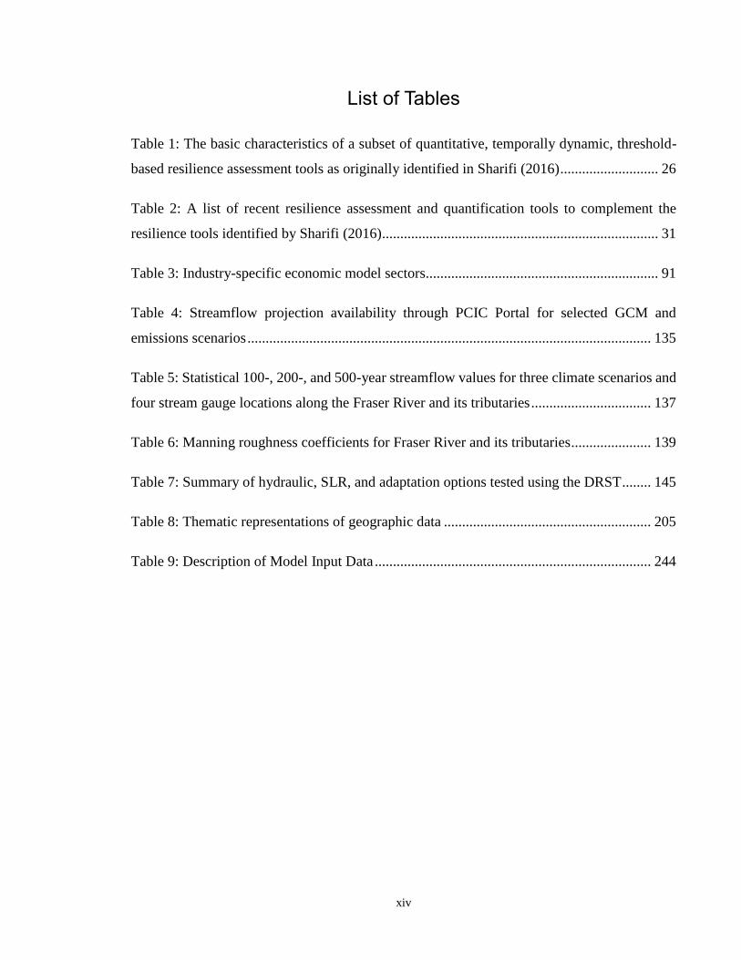
List of Tables
Table 1: The basic characteristics of a subset of quantitative, temporally dynamic, threshold-
based resilience assessment tools as originally identified in Sharifi (2016) ........................... 26
Table 2: A list of recent resilience assessment and quantification tools to complement the
resilience tools identified by Sharifi (2016)............................................................................ 31
Table 3: Industry-specific economic model sectors................................................................ 91
Table 4: Streamflow projection availability through PCIC Portal for selected GCM and
emissions scenarios ............................................................................................................... 135
Table 5: Statistical 100-, 200-, and 500-year streamflow values for three climate scenarios and
four stream gauge locations along the Fraser River and its tributaries ................................. 137
Table 6: Manning roughness coefficients for Fraser River and its tributaries ...................... 139
Table 7: Summary of hydraulic, SLR, and adaptation options tested using the DRST ........ 145
Table 8: Thematic representations of geographic data ......................................................... 205
Table 9: Description of Model Input Data ............................................................................ 244

xv
List of Figures
Figure 1: Projected population growth; red dots indicate megacities (≥ 10 million people)
(image from: (UN DESA, 2018)) ........................................................................................... 15
Figure 2: Framework for disaster resilience quantification and methodology for its
implementation ....................................................................................................................... 35
Figure 3: Conceptual definition of STDRM using system performance graph (modified after
Simonovic and Peck, 2013) .................................................................................................... 39
Figure 4: Illustration of dynamic system resilience in performance space ............................. 42
Figure 5: Illustration of dynamic system resilience in resilience space demonstrating examples
of resilience which returns to pre-shock levels (solid line); exceeds pre-shock levels (dash-dot
line); and does not recover to pre-shock levels (dotted line) .................................................. 43
Figure 6: Illustrative dynamic resilience map in time (t) and space (x,y) using STDRM where
the changing colours represent changes in resilience ............................................................. 44
Figure 7: Four types of threshold responses including (a) no response; (b) step-change; (c)
alternate stable state; and (d) irreversible change (adapted from Walker and Salt, 2012) ..... 46
Figure 8: Schematic example of a moving threshold.............................................................. 47
Figure 9: Schematic of conceptual thresholds in performance space for (a) Scenario A: higher
threshold; and (b) Scenario B: lower threshold ...................................................................... 48
Figure 10: A non-exhaustive example of multiple (hierarchical/vertical) multi-level
governance scales which may be involved in the mitigation, planning, response, or recovery
decisions and/or actions in the event of a natural disaster ...................................................... 51
Figure 11: Generic implementation methodology .................................................................. 55
Figure 12: Generic stock and flow diagram ............................................................................ 58
Figure 13: Technical implementation schematic for the DRST ............................................. 66
xvi
Figure 14: Generic model structure for each domain (I-n) ..................................................... 68
Figure 15: Physical domain workflow diagram; tasks 4, 5, and 6 are completed for each
unsteady flow simulation scenario .......................................................................................... 73
Figure 16: General river network digitization scheme (based on USACE (2011)) ................ 75
Figure 17: Pathways of global CO2 concentrations for AR5 emissions scenarios (from IPCC
(2013))..................................................................................................................................... 76
Figure 18: Simulation results of CO2 in the atmosphere if the land and ocean can no longer
absorb close to half of all climate-warming CO2 emissions (from NASA (2015)) ............... 76
Figure 19: Projected SLR for RCP 2.6 (lower, blue projected line) and RCP 8.5 (higher, red
projected line) (IPCC, 2013) ................................................................................................... 79
Figure 20: Climate model ensemble mean relative sea level change (m) (between 1986-2005
and 2081-2100) for (a) RCP 2.6; and (b) RCP 8.5 (adapted from IPCC (2013)) .................. 79
Figure 21: VIC hydrological modelling schematic (from Liang et al., (1994)) ..................... 82
Figure 22: River schematic identifying locations which require the specification of boundary
conditions and where climate change is incorporated into the hydraulic modelling process . 85
Figure 23: Schematic of physical domain output (a) generated from hydraulic unsteady flow
simulation; (b) when combined with spatial topographical information to generate a time series
of inundation maps (adapted from USACE 2010) ................................................................. 86
Figure 24: Schematic of spatial overlay and infrastructure attributes contributing to economic
CGE model.............................................................................................................................. 91
Figure 25: Schematic of the economics domain GAMS modelling and optimization; this
process is completed only once, at the end of the simulation ................................................. 93
Figure 26: Schematic of engineering domain calculations for a single infrastructure element
(adapted from Nastev and Todorov (2013)) ........................................................................... 95

xvii
Figure 27: Engineering resilience spatial implementation, direct damages workflow diagram
this process is completed for each time step (t) in the simulation .......................................... 97
Figure 28: Implementation of the spatial health domain cost-distance algorithm ................ 106
Figure 29: Health resilience spatial implementation, cost-distance workflow diagram; this
process is completed for each time step (t) in the simulation ............................................... 107
Figure 30: Social resilience spatial implementation, communications workflow diagram this
process is completed for each time step (t) in the simulation ............................................... 110
Figure 31: Region of Metro Vancouver (and population estimates) in the province of British
Columbia, Canada (inset image courtesy of Metro Vancouver (2017)) ............................... 115
Figure 32: Dissemination Areas (orange boundary lines) in the Region of Metro Vancouver
(white shaded area) ............................................................................................................... 115
Figure 33: A selection of spatial inputs collected for use in disaster resilience quantification as
part of the DRST ................................................................................................................... 120
Figure 34: Dynamic disaster resilience quantification Vensim model ................................. 121
Figure 35: Emergency funding component of the DRST Vensim model ............................. 121
Figure 36: Disaster resilience calculation component of the DRST Vensim model ............ 125
Figure 37: Metro Vancouver, the Fraser River, and its tributaries as: (a) a DEM of low
elevations (black shade) and high elevations (white shade); and (b) a TIN of low elevations
(blue colour) and high elevations (red colour) ...................................................................... 130
Figure 38: The four Water Survey of Canada gauge sites (08MH024; 08MF005; 08MH001;
08MG013) in British Columbia along the Fraser River and its tributaries (provided by Markus
Shnorbus, PCIC 2014) .......................................................................................................... 135
Figure 39: HEC-RAS model geometry (river centerline and cross sections) ....................... 140
Figure 40: Example of one of the cross sections from the HEC-RAS model....................... 140

xviii
Figure 41: A sample map of the cost-distance algorithm output used by the DRST in the
calculation of health resilience for one scenario (Baseline), for one time step (t=0); the ‘H’
symbols represent hospitals; yellow is low cost-distance, purple is high cost-distance ....... 147
Figure 42: Spatial engineering resilience for Scenario 2 across dissemination areas for Metro
Vancouver (14 total time steps); maps in NAD 83 CRCS ................................................... 150
Figure 43: Engineering resilience at one time step (t = 7) for (a) Scenario 1; (b) Scenario 2;
and (c) Scenario 5 near the Fraser River in the member municipalities of Coquitlam, Surrey,
and Pitt Meadows .................................................................................................................. 151
Figure 44: Spatial health resilience for Scenario 2 across dissemination areas in Metro
Vancouver (14 total time steps); maps in NAD 83 CRCS ................................................... 155
Figure 45: Hospitals (non-auxiliary) near the City of Delta ................................................. 155
Figure 46: Health resilience at one time step (t = 7) for (a) Scenario 1; (b) Scenario 2; and (c)
Scenario 4 for the cities of Richmond, Delta, Surrey, and White Rock ............................... 156
Figure 47: Spatial social resilience for Scenario 2 across dissemination areas in Metro
Vancouver (14 total time steps); maps in NAD 83 CRCS ................................................... 160
Figure 48: Difference in social system impacts for one time step (t = 4) for (a) Scenario 1; and
(b) Scenario 2 ........................................................................................................................ 161
Figure 49: Engineering resilience (Metro Vancouver) ......................................................... 163
Figure 50: Social resilience (Metro Vancouver) ................................................................... 164
Figure 51: Health resilience (Metro Vancouver) .................................................................. 165
Figure 52: Economic resilience (Metro Vancouver) ............................................................ 166
Figure 53: Economic resilience modelled over a longer (nearly 4 year) time period ........... 167
Figure 54: Total resilience (Metro Vancouver) .................................................................... 168
Figure 55: Spatial data as layers ........................................................................................... 205
xix
Figure 56: Two types of spatial data structures representing (a) spatially discrete features as
vector data; and (b) spatially continuous data as raster data ................................................. 207
Figure 57: Representation of spatially discrete features as (a) vector data; and (b) raster data
............................................................................................................................................... 207
Figure 58: Spatially discrete features (houses) represented in various vector formats (a) points;
(b) lines; and (c) polygons .................................................................................................... 208
Figure 59: Extract analysis tools (a) clip, (b) select, and (c) split ........................................ 211
Figure 60: A subset of the overlay analysis tools (a) union; (b) intersect; and (c) erase ..... 212
Figure 61: Cost distance proximity analysis ......................................................................... 213
Figure 62: Spatial raster reclassification ............................................................................... 214
Figure 63: Schematic of a geometric network ...................................................................... 215
Figure 64: Schematic of geometric network with flow direction ......................................... 216
Figure 65: Flags (sources), barriers, and weights ................................................................. 216
Figure 66: Conceptual results from a trace downstream operation in a geometric network 217
Figure 67: Structure of a GAMS program ............................................................................ 230
Figure 68: Organization of GAMS program ......................................................................... 231
Figure 69: Flow split assumptions for the Fraser River and its tributaries ........................... 249
Figure 70: Jacob Haldi Bridge from Fort Langley to McMillan Island, BC (Google Maps, 2014)
............................................................................................................................................... 251
Figure 71: DRST graphical user interface (GUI) screen ...................................................... 255

xx
List of Appendices
Appendix A An Introduction to Spatial Data, Spatial Data Tools, and their use in the
Development of the DRST.................................................................................................... 203
Appendix B VIC Hydrologic Model Equations.................................................................... 218
Appendix C HEC-RAS Hydraulic Modelling Equations ..................................................... 226
Appendix D GAMS Programming and Documentation ....................................................... 229
Appendix E Data to Support the Application of Resilience Quantification Framework for
Metro Vancouver, British Columbia, Canada ....................................................................... 243
Appendix F Disaster Resilience Simulation Tool (DRST) and Python Code ..................... 247
Appendix G Fraser River Hydraulic Modelling Assumptions and Limitations ................... 248
Appendix H Disaster Resilience Simulation Tool (DRST) Graphical User Interface (GUI)
............................................................................................................................................... 254
Appendix I Curriculum Vitae .............................................................................................. 259

xxi
Acronyms and Terminology
ABM Agent Based Model
API Application Programming Interface
AR4 IPCC’s Fourth Assessment Report
AR5 IPCC’s Fifth Assessment Report
BC Boundary Condition
BC British Columbia
BCA British Columbia Assessment [Corporation]
BCSD Bias Corrected Spatial Disaggregation
CGE Computable General Equilibrium [model]
CLARA Coastal Louisiana Risk Assessment Model
DA Dissemination Area
DALY Disability Adjusted Life Year
DEM Digital Elevation Model
DLL Dynamic Library Link
DMAF Disaster Mitigation and Adaptation Fund
DRST Disaster Resilience Simulation Tool
EPA Environmental Protection Agency
ESRI Environmental Systems Research Institute
xxii
FBC Fraser Basin Council
GAMS General Algebraic Modeling System
GCM Global Climate Model
GCS Geographic Coordinate System
GDP Gross Domestic Product
GFDRR Global Facility for Disaster Reduction and Recovery
GHG Greenhouse Gases
GIS Geographic Information System
GMSL Global Mean Sea Level
GUI Graphical User Interface
HEC-GeoRAS the Hydrologic Engineering Centers Geographic River Analysis System
HEC-RAS the Hydrologic Engineering Centers River Analysis System
HFA Hyogo Framework for Action
ICIP Investing in Canada Infrastructure Program
IPCC Intergovernmental Panel on Climate Change
LiDAR Light Detection and Ranging
MFLNRO Ministry of Forests, Lands and Natural Resource Operations
MGI McKinsey Global Institute
NASA National Aeronautics and Space Administration
xxiii
NGO Non-Governmental Organization
NHC Northwest Hydraulic Consultants
PAHO Pan American Health Organization
PCIC Pacific Climate Impacts Consortium
PCS Projected Coordinate System
PIF Performance Influencing Factors
RCM Regional Climate Model
RCP Representative Concentration Pathway
SAM Social Accounting Matrix
SD System Dynamics
SLR Sea Level Rise
SRES Special Report on Emissions Scenarios [scenarios]
STDRM Space-Time Dynamic Resilience Measure
SWAT Soil Water Assessment Tool
UN DESA United Nations Department of Economic and Social Affairs
UNISDR United Nations International Strategy for Disaster Risk Reduction
USACE United States Army Corps of Engineers
VIC Variable Infiltration Capacity [model]
WHO World Health Organization

1
Chapter 1
1 INTRODUCTION
Cities are complex systems facing a diverse set of issues including: rapid population
growth; environmental threats; resource shortages; social inequalities; disruptive
technologies; and complex governance. The World Economic Forum anticipates that by
2050 over 68% of the global population will live in urban areas (UN DESA, 2018) which
will only exacerbate existing problems. As cities progressively increase in size and
complexity, good governance and decision making will be imperative to managing the
demands, threats, and sustainability of urban systems.
Over the last several decades, cities have faced a diverse set of issues. Coastal cities in
particular must manage the growing threat of sea level rise and the impacts of climate
change on hydrometeorological hazards. Extreme variations in the hydrologic cycle, in
addition to long-lasting alterations of physical conditions and urban intensification, can
impact environmental, economic, engineering, health, and social systems causing
devastation to a city.
This chapter introduces disaster management approaches and climate change-influenced
hazards. It outlines the main objectives, research questions, and contributions of this work
to the scientific and disaster management communities.
1.1 Risk to Resilience: A Changing Disaster Management Paradigm
There are practical links between disaster risk management, climate change adaptation, and
sustainable development that lead to reduction of disaster risk and reinforce resilience as a
new development paradigm (de Bruijn et al., 2017). The past couple of decades have
experienced a noticeable change in disaster management approaches; a switch from
traditional disaster risk and vulnerability reduction strategies to progressive disaster
resilience development strategies. Traditional risk and vulnerability approaches focus on
system deficiencies whereas resilience approaches are a more proactive and positive

2
expression of community engagement within natural disaster management. A resilience
approach focuses on the inherent and adaptive coping capacities of a community and places
an emphasis on local strengths and opportunities to “build back better” (Clinton, 2006;
Gupta, et al., 2010; Fan, 2013; World Health Organization, 2013). In the past, disaster
management planning emphasized the documentation of roles, responsibilities, and
procedures. Increasingly, these plans consider arrangements for prevention, mitigation,
preparedness, response, and recovery. However, over the last ten years, substantial
progress has been made in establishing the role of resilience as part of sustainable disaster
management (Adger, 2007, Nelson et al., 2007). Multiple case studies around the world
reveal links between attributes of resilience and the capacity of complex systems to absorb
disturbances while still maintaining a certain level of functioning. There is a need to focus
more on action-based resilience planning to strengthen local capacity and capability,
including a greater emphasis on community engagement, to gain a better understanding of
the diversity, needs, strengths, and vulnerabilities within communities. This research
recognizes the paradigm shift from disaster risk to resilience and formalizes the qualitative
and quantitative definition of resilient systems. This research also demonstrates a
mechanism by which disaster resilience can be represented and quantified.
Disasters do not impact every community in the same way. It is clear that problems
associated with sustainable human wellbeing in urban regions calls for new scientific and
practical approaches. Cities may be viewed as living systems (i.e. a systems of systems),
constantly self-organizing in many varied ways in response to both internal interactions
and the influence of external factors. Resilience is an appropriate matrix for investigation
considering the essential overlaps between the built environment, physical environment,
social dynamics, metabolic flows, and governance networks (Simonovic and Peck, 2013).
This research seeks to address the need to model the complex interdependencies of urban
systems as they relate to disaster resilience. Furthermore, this research incorporates the
diversity of urban regions and recognizes the importance of formulating resilience-based
strategies in a local context. Therefore, although the resilience theory and methodology
presented may be generally applied to any region, the application of a resilience simulator
tool presented in this research was developed specific to Metro Vancouver, British
Columbia, Canada.
3
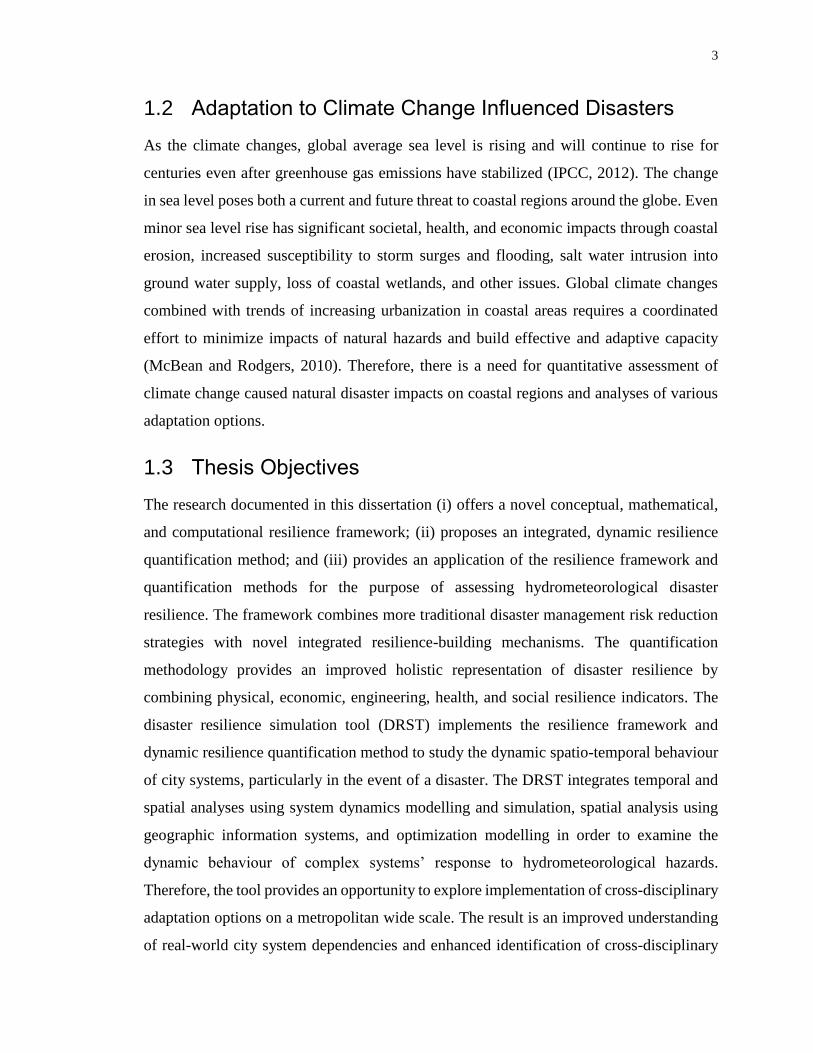
1.2 Adaptation to Climate Change Influenced Disasters
As the climate changes, global average sea level is rising and will continue to rise for
centuries even after greenhouse gas emissions have stabilized (IPCC, 2012). The change
in sea level poses both a current and future threat to coastal regions around the globe. Even
minor sea level rise has significant societal, health, and economic impacts through coastal
erosion, increased susceptibility to storm surges and flooding, salt water intrusion into
ground water supply, loss of coastal wetlands, and other issues. Global climate changes
combined with trends of increasing urbanization in coastal areas requires a coordinated
effort to minimize impacts of natural hazards and build effective and adaptive capacity
(McBean and Rodgers, 2010). Therefore, there is a need for quantitative assessment of
climate change caused natural disaster impacts on coastal regions and analyses of various
adaptation options.
1.3 Thesis Objectives
The research documented in this dissertation (i) offers a novel conceptual, mathematical,
and computational resilience framework; (ii) proposes an integrated, dynamic resilience
quantification method; and (iii) provides an application of the resilience framework and
quantification methods for the purpose of assessing hydrometeorological disaster
resilience. The framework combines more traditional disaster management risk reduction
strategies with novel integrated resilience-building mechanisms. The quantification
methodology provides an improved holistic representation of disaster resilience by
combining physical, economic, engineering, health, and social resilience indicators. The
disaster resilience simulation tool (DRST) implements the resilience framework and
dynamic resilience quantification method to study the dynamic spatio-temporal behaviour
of city systems, particularly in the event of a disaster. The DRST integrates temporal and
spatial analyses using system dynamics modelling and simulation, spatial analysis using
geographic information systems, and optimization modelling in order to examine the
dynamic behaviour of complex systems’ response to hydrometeorological hazards.
Therefore, the tool provides an opportunity to explore implementation of cross-disciplinary
adaptation options on a metropolitan wide scale. The result is an improved understanding
of real-world city system dependencies and enhanced identification of cross-disciplinary

4
system interactions in the event of a disaster. Simulations using the DRST provide insight
into the spatial and temporal patterns of resilience. Through testing various adaptation
options, the DRST can help guide disaster management decision making.
Therefore, the main goal of the presented research is development of a tool that allows
simulation of disaster resilience policy scenarios (also called adaptation scenarios) and
observation of changes in resilience behavior over both time and space in the event of a
hydrometeorological natural disaster. Simulating dynamic resilience behavior in response
to various policy actions helps to: identify disaster-resilient systems; determine why some
systems are more resilient than others; and prioritize adaptation actions. Thus, the main
objectives of this research are as follows:
1. To provide a framework for dynamic spatio-temporal representation of disaster
resilience;
2. To develop a framework for combining multiple domains of disaster resilience
to offer a more holistic representation of disaster resilience;
3. To provide a mechanism for quantifying disaster resilience;
4. To develop a modelling tool which simulates dynamic space-time disaster
resilience using the temporal modelling and simulation capabilities of system
dynamics (SD) combined with the spatial analysis capabilities of geographic
information systems (GIS); and
5. To test and assess various adaptation policies in the context of disaster
resilience.
The purpose of pursing this research is to gain insight into the following research questions:
1. Are coastal cities becoming more (or less) resilient to natural disasters?
2. What factors contribute most (and least) to disaster resilience?

5
3. Which systems are least (and most) resilient? In which disaster phase are they
least (and most) resilient? Where are these system deficiencies (and strength
and opportunities) located?
4. Which strategies may offer coastal cities the best opportunities to adapt to and
cope with the impacts of climate-change influenced hazards?
To obtain the answers to these questions, the concept of disaster resilience is used as a
measure by which to analyze and compare various climate change adaptation strategies.
An original framework is developed for the quantification of dynamic resilience through
integrated spatio-temporal system dynamics, geographic information systems, and
economics optimization to assess the impacts of climate change on coastal megacities. A
quantitative, Space-Time Dynamic Resilience Measure (STDRM) is used as a measure of
resilience which combines economic, engineering, health, physical, and social impacts of
disasters. A resilience simulator tool (DRST) was developed which uses the STDRM
calculation, combined with other spatio-temporal tools and methods, to simulate dynamic
spatio-temporal resilience behaviour of city systems.
1.4 Thesis Contributions to Research
Resilience-based approaches to disaster management offer a framework for deeper
engagement on the behaviour of complex adaptive systems. While the concept of resilience
in disaster management is not new, methods and frameworks for resilience quantification
remain in its infancy. Furthermore, while there is general agreement in the scientific
community that resilience involves spatial and temporal dynamic processes, there is a
limited research describing just how to capture them.
While the resilience concept has gained momentum in disaster management literature, most
of the discussion revolves around qualitative descriptions of resilience; few attempts have
been made to resilience quantification and much research is still required to fill this gap.
This research offers a pioneering effort in dynamic disaster resilience quantification,
modelling, and simulation to help advance the fields of system dynamics simulation,

6
climate change adaptation, and disaster resilience theory, methods, and applications. The
more specific contributions of this work are as follows:
Theoretical and Analytical contributions
1. Resilience definition, quantification method, and assessment that is dynamic in
both time and space (work published in Simonovic and Peck, 2013);
2. A methodological and computational framework and analysis method for
dynamic disaster resilience quantification;
3. A methodological framework that enables the integration of multiple disaster
resilience domains including interrelated physical, economic, engineering,
health, and social disaster impacts and capacities used to provide a
comprehensive description of disaster resilience;
4. The integration of system dynamics simulation, economic optimization, and
geographic information systems methods and tools for dynamic spatio-temporal
resilience simulation and mapping (foundations of this work published in
Neuwirth et al., (2015));
Computational contributions
5. Disaster resilience quantification with the ability to capture system
improvements in the process of recovery (i.e. recovery levels exceeding pre-
disaster levels);
6. Disaster resilience quantification with the ability to capture the impact of
performance thresholds;
Additional contributions
7. A middleware program designed to communicate between a system dynamics
simulation model (created in Vensim software (Ventana Systems Inc., 2009)),
an economics optimization model (created using the General Algebraic

7
Modelling System (GAMS) software (GAMS Development Corporation,
1987)), and spatial data analysis models (created in ArcGIS software (ESRI,
2011)); and
8. A proof-of-concept application of the proposed resilience quantification
framework and methodology to Metro Vancouver in British Columbia, Canada.
1.5 Thesis Organization
The following chapters focus on the procedure for developing a framework, methodology,
and tool to quantify and assess resilience to climate change influenced hydrometeorological
disasters.
Chapter 2 examines the state of climate change and disaster management research. An
argument is made for a paradigm shift in the disaster management community from risk to
resilience, as traditional risk assessment approaches are no longer suitable decision making
tools in the face of a changing climate. As awareness and acknowledgement of climate
change impacts grow in the scientific and political communities, there is an increasing
demand for disaster resilience quantification methods and tools to provide additional
insight into effective disaster management strategies. Although there is significant
literature available on resilience concepts, research in this area has often been siloed within
specific scientific fields. Therefore, resilience concepts are explored through a variety of
scientific fields and are integrated to form a comprehensive definition of dynamic disaster
resilience. The second part of this chapter introduces system dynamics modelling and
simulation which is used to capture complex temporal non-linear feedbacks within
systems.
Chapter 3 focuses on resilience theory and the resilience quantification methods. This
chapter sets the resilience landscape and characterizes dynamic disaster resilience. One of
the defining characteristics and strengths of the disaster resilience principle, as identified
in this chapter, is its ability to represent dynamics in both time and space. To capture these
dynamics, spatial and temporal modelling techniques are integrated into a novel resilience
simulation tool (DRST). This tool captures the linkages and interactions within, and

8
between, five model domains (physical, economics, engineering, health, and social) to
simulate a city’s response following a disruption (in this case, a flood). The end of this
chapter provides a conceptual introduction to the DRST.
Chapter 4 focuses on the implementation of the dynamic disaster resilience quantification
methodology and dynamic resilience mathematical concept. This chapter provides a
detailed description of the DRST including a description of each of the models’ systems
and subsystems. The DRST consists of one input domain (physical hazard) and four
integrated impact domains: economic, engineering, health, and social. The main structure
of each of the four impact domains is similar, but the way in which resilience is
characterized and quantified for each of these domains varies greatly. The development of
each of the five domains, relative to the resilience focal scale, is discussed in this chapter.
Chapter 5 describes an application of the framework and implementation of the resilience
quantification methodology using the DRST in a Canadian context for the region of Metro
Vancouver in British Columbia, Canada. This application tests three different adaptation
strategies: mobile health unit, managed retreat, and access to additional external funding
to examine their effects on disaster resilience. The DRST provides insight into which of
these adaptation options may provide the greatest opportunity to improve regional disaster
resilience.
Chapter 6 summarizes the findings and limitations of the concepts and applications
presented in this dissertation and provides recommendations for future research related to
the refinement, modification, expansion, and continuation of the DRST and proposes
recommendations for adopting resilience-based strategies in the disaster management
community.
9
Chapter 2
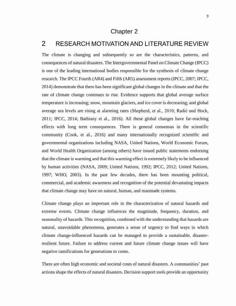
2 RESEARCH MOTIVATION AND LITERATURE REVIEW
The climate is changing and subsequently so are the characteristics, patterns, and
consequences of natural disasters. The Intergovernmental Panel on Climate Change (IPCC)
is one of the leading international bodies responsible for the synthesis of climate change
research. The IPCC Fourth (AR4) and Fifth (AR5) assessment reports (IPCC, 2007; IPCC,
2014) demonstrate that there has been significant global changes in the climate and that the
rate of climate change continues to rise. Evidence supports that global average surface
temperature is increasing; snow, mountain glaciers, and ice cover is decreasing; and global
average sea levels are rising at alarming rates (Shepherd, et al., 2010; Radić and Hock,
2011; IPCC, 2014; Bathiany et al., 2016). All these global changes have far-reaching
effects with long term consequences. There is general consensus in the scientific
community (Cook, et al., 2016) and many internationally recognized scientific and
governmental organizations including NASA, United Nations, World Economic Forum,
and World Health Organization (among others) have issued public statements endorsing
that the climate is warming and that this warming effect is extremely likely to be influenced
by human activities (NASA, 2009; United Nations, 1992; IPCC, 2012; United Nations,
1997; WHO, 2003). In the past few decades, there has been mounting political,
commercial, and academic awareness and recognition of the potential devastating impacts
that climate change may have on natural, human, and manmade systems.
Climate change plays an important role in the characterization of natural hazards and
extreme events. Climate change influences the magnitude, frequency, duration, and
seasonality of hazards. This recognition, combined with the understanding that hazards are
natural, unavoidable phenomena, generates a sense of urgency to find ways in which
climate change-influenced hazards can be managed to provide a sustainable, disaster-
resilient future. Failure to address current and future climate change issues will have
negative ramifications for generations to come.
There are often high economic and societal costs of natural disasters. A communities’ past
actions shape the effects of natural disasters. Decision support tools provide an opportunity
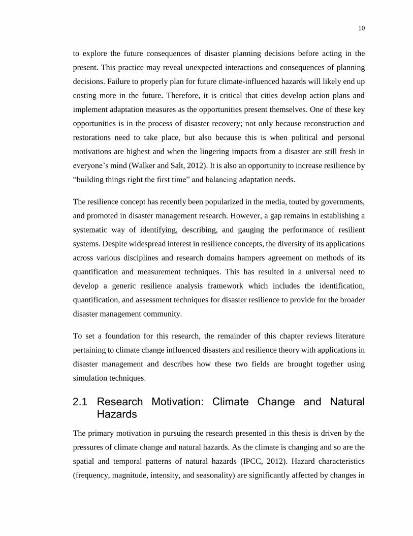
10
to explore the future consequences of disaster planning decisions before acting in the
present. This practice may reveal unexpected interactions and consequences of planning
decisions. Failure to properly plan for future climate-influenced hazards will likely end up
costing more in the future. Therefore, it is critical that cities develop action plans and
implement adaptation measures as the opportunities present themselves. One of these key
opportunities is in the process of disaster recovery; not only because reconstruction and
restorations need to take place, but also because this is when political and personal
motivations are highest and when the lingering impacts from a disaster are still fresh in
everyone’s mind (Walker and Salt, 2012). It is also an opportunity to increase resilience by
“building things right the first time” and balancing adaptation needs.
The resilience concept has recently been popularized in the media, touted by governments,
and promoted in disaster management research. However, a gap remains in establishing a
systematic way of identifying, describing, and gauging the performance of resilient
systems. Despite widespread interest in resilience concepts, the diversity of its applications
across various disciplines and research domains hampers agreement on methods of its
quantification and measurement techniques. This has resulted in a universal need to
develop a generic resilience analysis framework which includes the identification,
quantification, and assessment techniques for disaster resilience to provide for the broader
disaster management community.
To set a foundation for this research, the remainder of this chapter reviews literature
pertaining to climate change influenced disasters and resilience theory with applications in
disaster management and describes how these two fields are brought together using
simulation techniques.
2.1 Research Motivation: Climate Change and Natural Hazards
The primary motivation in pursuing the research presented in this thesis is driven by the
pressures of climate change and natural hazards. As the climate is changing and so are the
spatial and temporal patterns of natural hazards (IPCC, 2012). Hazard characteristics
(frequency, magnitude, intensity, and seasonality) are significantly affected by changes in
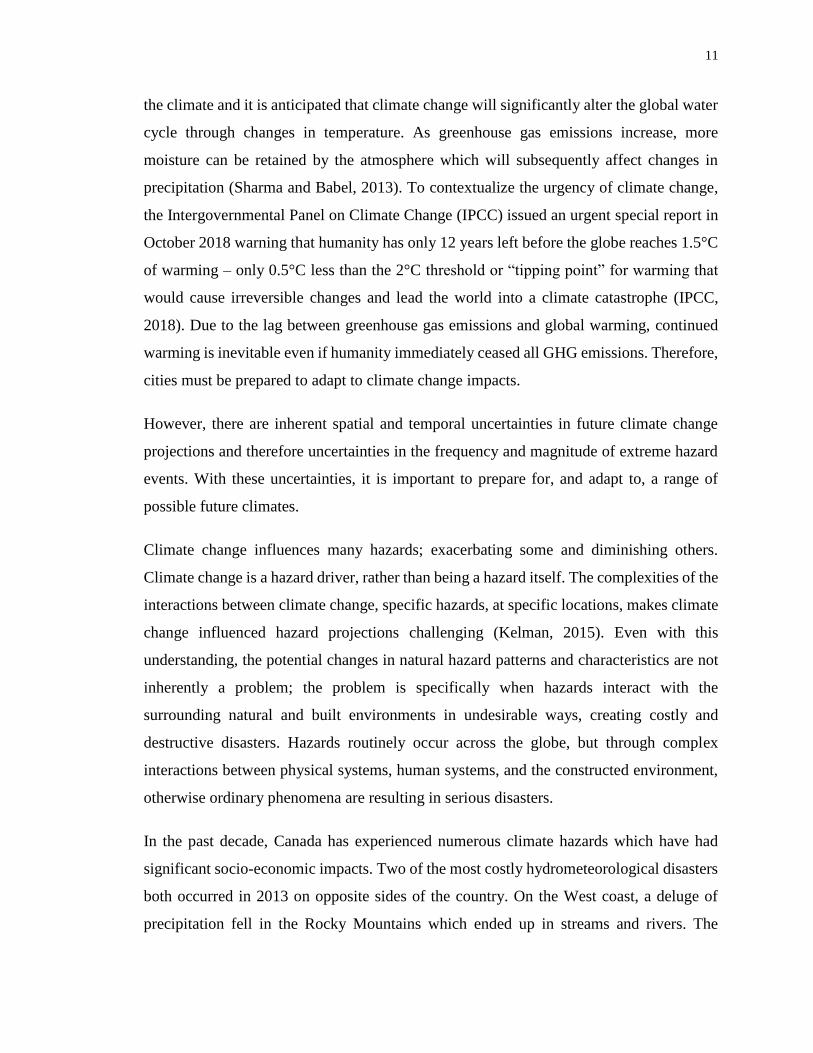
11
the climate and it is anticipated that climate change will significantly alter the global water
cycle through changes in temperature. As greenhouse gas emissions increase, more
moisture can be retained by the atmosphere which will subsequently affect changes in
precipitation (Sharma and Babel, 2013). To contextualize the urgency of climate change,
the Intergovernmental Panel on Climate Change (IPCC) issued an urgent special report in
October 2018 warning that humanity has only 12 years left before the globe reaches 1.5°C
of warming – only 0.5°C less than the 2°C threshold or “tipping point” for warming that
would cause irreversible changes and lead the world into a climate catastrophe (IPCC,
2018). Due to the lag between greenhouse gas emissions and global warming, continued
warming is inevitable even if humanity immediately ceased all GHG emissions. Therefore,
cities must be prepared to adapt to climate change impacts.
However, there are inherent spatial and temporal uncertainties in future climate change
projections and therefore uncertainties in the frequency and magnitude of extreme hazard
events. With these uncertainties, it is important to prepare for, and adapt to, a range of
possible future climates.
Climate change influences many hazards; exacerbating some and diminishing others.
Climate change is a hazard driver, rather than being a hazard itself. The complexities of the
interactions between climate change, specific hazards, at specific locations, makes climate
change influenced hazard projections challenging (Kelman, 2015). Even with this
understanding, the potential changes in natural hazard patterns and characteristics are not
inherently a problem; the problem is specifically when hazards interact with the
surrounding natural and built environments in undesirable ways, creating costly and
destructive disasters. Hazards routinely occur across the globe, but through complex
interactions between physical systems, human systems, and the constructed environment,
otherwise ordinary phenomena are resulting in serious disasters.
In the past decade, Canada has experienced numerous climate hazards which have had
significant socio-economic impacts. Two of the most costly hydrometeorological disasters
both occurred in 2013 on opposite sides of the country. On the West coast, a deluge of
precipitation fell in the Rocky Mountains which ended up in streams and rivers. The

12
steepness of the terrain caused flows to route quickly downstream and combine with a
record-high 45 mm of daily rainfall. By June 20th, over 100,000 people had been evacuated
and the city of Calgary was inundated with floodwaters up to 2 m high (Pomeroy et al.,
2016). Flood waters caused widespread damage to telecommunications, transportation
corridors, power utilities, properties, and caused four casualties. Two weeks later on July
8th 2013, the city of Toronto faced an intense thunderstorm which brought 126 mm of
precipitation to the region causing flash flooding, catching most local residents unprepared
(Environment Canada, 2013). The disaster caused wide-spread damages to properties,
disruptions to transportation, and interruption of utility services. Since then, there have
been a number of other major flooding disasters including the 2017 flooding of the Grand
River and the most recent 2019 flooding of the Ottawa River.
These disasters highlight the catastrophic effects that hydrometeorological disasters can
have, even in interior Canada. Climate changes and land use patterns are driving changes
in Canada’s flood regime (Burn and Whitfield, 2016). The 2013 event in southern Alberta
was determined to be a 1- in approximately 40-year event (Pomeroy et al., 2016). However,
with the changing climate it is possible that what was historically the 1- in 40-year flood
event may now be closer to a 1 in 25-year event; and looking to the future, it’s possible
that the frequency of high precipitation events may increase even further (IPCC, 2014).
What’s more, Canadian cities at the confluence of riverine and ocean (delta) environments
face additional hazards. Coastal cities along river deltas operate in complex
hydrometeorological physical environments. They face pressures from: coastal hazards
such as hurricanes, tsunamis, and storm surge; riverine and estuary hazards such as water
salinization and fluvial flooding; and storm hazards such as pluvial flooding. At the global
scale, many other cities are facing similar problems.
Coastal regions are highly dynamic and complex systems which respond in various ways
to extreme weather events (Balica et al., 2012; Kerle and Muller, 2013). Coastal cities are
exposed to multiple types of extreme climate hazards, particularly hydrometeorological
hazards including storm surges, floods, hurricanes, sea level rise, and tsunamis. Recently,

13
there have been disasters affecting coastal cities across the globe resulting in significant
economic and social losses.
Since natural hazards are phenomena which cannot be entirely eliminated, it is necessary
to take measures to reduce the impacts on populations exposed to extreme climate hazards
through employing effective adaptation policy (Henstra, 2012). As adaptation mechanisms,
communities should consider increasing their flexibility, resistance, and robustness to cope
with the various impacts of extreme hazards (Godschalk, 2003) and integrate adaptive
capacity into the fabric of society (Paton and Johnston, 2006).
Climate change modelling is typically employed to help improve the understanding of
relationships and identify important feedbacks in the complex climate-earth system.
Climate models provide estimates of how physical systems will respond under various
carbon emissions scenarios. The IPCC AR4 (2007) and AR5 (2014) reports outline
scenarios which range from a carbon emissions “reduction” future scenario to the less
conservative “business as usual” carbon emissions scenario. These emissions scenarios are
used in conjunction with Global Climate Models (GCMs) in climate modelling to provide
estimates of potential future warming of the Earth’s atmosphere. Although GCM outputs
provide a reasonable estimation of future climate, their coarse spatial resolution is limiting
in many local and regional applications. When a finer spatial resolution is required,
statistical or dynamic regional climate model (RCM) downscaling techniques are used to
bring GCM output to the local level (Masud et al., 2016).
Furthermore, to determine how greenhouse gas (GHG) emissions and atmospheric climate
changes may modify hydrometeorological hazards, the GCM or RCM outputs are used in
hydrologic and hydraulic modelling applications (Arnell, et al., 2001; Shrestha, 2014; Eum
et al., 2010) to estimate how climate scenarios may modify streamflows, water levels, and
flood extents. This research applies a similar methodology to estimate climate change
influenced flooding. These floods represent future possible events under climate change.
Even though the resilience framework and methodology presented in this research can be
generically applied to any city, the climate change influenced hazards will vary according
to future estimated regional hydrometeorological conditions of the basin.
14
Climate change and urbanization are considered the main motivations of this research.
With increased urban pressures and catastrophic climate threats looming on the not-too-
distant horizon, it is more important than ever for cities to make informed, long-term
decisions and become more resilient.
2.2 Research Motivation: Megacities
Another primary driver of the research presented in this thesis was due to the pressures of
rapid urbanization and the increasing size and complexity of the world’s megacities. When
it comes to the rapid urbanization of coastal megacities, the only constant is change. It’s
projected that 68% of the global population will be living in urban areas by 2050; an
increase of approximately 30% from global urban population levels in 2011 (UN DESA,
2018). This anticipated increase may be attributed to the trend of increasing rural-to-urban
migration as people abandon agricultural practices to seek out economic opportunities and
prosperity in urban cities (Wenzel et al., 2007; Akanda and Hossain, 2012). This migration
is causing many major cities to rapidly develop into megacities (Akanda and Hossain,
2012); defined by the United Nations as cities with populations greater than 10 million
people (UN DESA, 2018). The number of global megacities is anticipated to grow to 43;
most of them in developing regions. As supported by Figure 1, a majority of the world’s
current and projected megacities are located in hazardous low-lying coastal areas,
particularly in developing countries (Akanda and Hossain, 2012; UN DESA, 2018).
Therefore, millions of people are already exposed to coastal climate hazards. In addition,
these megacities are often characterized by high population densities, destitute slum
settlements, and inadequate life-sustaining infrastructure (Wenzel et al., 2007); conditions
which exacerbate the impacts of climate hazards. Currently, 21% of the world’s population
lives within coastal zones and an average of 46 million people per year experience storm
surge flooding. Some 189 million people presently live below the 1 in 100-year storm surge
level. To exacerbate this problem, some coastal megacities are expected to experience more
frequent, high intensity events in the future as a result of the changing climate. In addition
to more immediate hazards that threaten coastal cities, it is expected that many coastal
cities will see some degree of sea level rise (SLR) in the future (Hinkel, et al., 2014; Wong,
et al., 2014; Jevrejeva et al., 2016; Bindoff, et al., 2007). Land subsidence combined with

15
warming is causing SLR at unprecedented rates (Wong, et al., 2014). Even if global
emissions were immediately reduced to zero, emissions retained by the atmosphere would
cause the globe to continue to warm. Jevrejeva et al. (2016) estimates that with even 2°C
of warming, more than 90% of coastal areas would exceed 0.2 m of SLR by 2040. If
warming were to exceed this estimate (which is a distinct possibility), SLR levels would
be even higher. These small changes in SLR play a significant role in the magnitude and
extent of flooding due to storm surges. Higher sea levels are not just a problem of additional
water, but also salt contamination. Salt water flooding has the potential to negatively
impact agricultural land, groundwater, and freshwater ecosystems.
Figure 1: Projected population growth; red dots indicate megacities
(≥ 10 million people)
(image from: (UN DESA, 2018))
Megacities possess a diverse set of intellectual, technical, and financial resources that,
when mobilized effectively, provide an opportunity to develop effective disaster resilient
systems.

16
The many disaster management professionals still operate with a reductionist approach to
handling complex systems by breaking them down into small, separate, manageable
components. This approach enforces the perception that these components are unrelated to
each other. A shift in thinking from a compartmentalized approach to a more holistic,
interrelated way is required to tackle large-scale issues such as climate change and disaster
management. The essence of systems thinking is wholeness. The objective is to look at the
behavior of interrelated non-linear systems together to better understand those relationships
which influence complex system behavior.
Orr (2014) suggests there are at least 6 ways in which systems thinking can help improve
urban governance:
1. Help governments organize data to distinguish between information and noise
2. Educate the citizens
3. Improve forecasting and planning
4. Improve the quality of urban decision-making
5. Improve organizational behavior
6. Improve realism and precautionary public policies
Thus, systems thinking is a critical component to building sustainable and resilient cities.
Cities can be thought of as systems of systems. That is, a city is made of many sub-systems,
each consisting of its own components, but interacting dynamically with other city sub-
systems to form the complex whole which allows a city to function. This approach brings
up another important systems concept: that constitutive characteristics are not explainable
from the characteristics of isolated parts. That is, merely adding up the components is
meaningless as compared to the part-whole relationships and the collective behaviour of
the system. Applying conventional thinking to complex problems, can lead to unintended
consequences. Fixing isolated pieces without consideration for the whole may seem
harmless, but also may be ignoring essential relationships that drive system behaviour and
end up undermining the best efforts of the solution. In an ever growing, advancing, and

17
globalized society, systems thinking is essential for developing effective solutions to
complex real-world problems. The rise of cities in the world presents both opportunities
and potential problems. The challenge for social system design is summarized in the second
McKinsey Global Institute (MGI) report:
“Cities can be part of the solution to such stresses, as concentrated population center can
be more productive in their resource use than areas that are more sparsely populated. But
if cities fail to invest in a way that keeps abreast of the rising needs of their growing
populations, they may lock in inefficient, costly practices that will become constraints to
sustained growth later on. How countries and cities meet this rising urban demand
therefore matters a great deal. Beyond the direct impact of the investment, their choices
will have broad effects on global demand for resources, capital investment, and labor
market outcomes” (Dobbs, et al., 2012, p. 2).
Systems analysis is an approach used to break complex systems into its constituents and
study their interrelationships and function as part of the whole. The function of each
component in a systemic context differs from how the component would function in
isolation. Both cognitive (mental) and physical (mathematical) modelling techniques are
useful for formalizing system architecture and exploring emergent system behaviour.
Cognitive models (e.g. causal loop diagrams) are mental models which help formalize and
visualize complex system structures; readily recognize relationships between system
elements; and identify feedback mechanisms that drive complex system behaviour.
Cognitive modelling is an important step in formalizing system structures. Causal loop
models are constructed based on research, personal experience, and in consultation with
experts and stakeholders in the fields of the system (and sub-systems) of interest. Mental
models are continually reassessed and refined as new information becomes available.
Mathematical and computer models (e.g. stock and flow diagrams) are idealized
representations of physical systems expressed in the form of mathematical expressions and
equations. Mathematical and computer models can simulate the complex relationships
between various elements within a system and give rise to resulting emergent system
behaviour.
18
2.3 Research Motivation: Disaster Resilience
Coastal urban development pressures, combined with increases in the magnitude and
frequency of climate change influence on coastal hazards, place a particular importance on
effective disaster management. It is imperative to estimate and reduce climate change
influenced hazard impacts by understanding the risks, vulnerabilities, and capacities of
people and the built environment to properly prepare for, and make informed decisions
related to, disaster management.
Historically, traditional approaches such as vulnerability assessments and “hard”
engineering mitigation measures, such as dikes, were the primary solutions to disaster
management problems. In other words, to prevent flooding, solutions would revolve
around building flood protection infrastructure stronger, bigger, and higher. However, it is
becoming apparent that flood protection infrastructure is only part of the solution and that
resilience approaches are key to finding more sustainable disaster management solutions.
The past two decades of disaster management have experienced a paradigm shift from
traditional disaster mitigation and prevention strategies to disaster resilience. This more
holistic approach has gained a lot of momentum in the disaster management community.
The benefit of this transition to resilience-based approaches is reinforced by social
scientists and psychologists who suggest that to tackle climate-related issues, the focus
should change from telling “catastrophe” stories to focusing on potential opportunities and
solutions; ways in which improvements can be made to new and existing systems to better
prepare, respond to, and recover from disasters. The resilience of people, nature, and the
built environment are all positive narratives which can drive constructive changes and help
build better cities (Goldstein et al., 2015).
Resilience focuses on positive characteristics and opportunities to improve or (in some
instances) transform a system. It is both a short-term response and long-term process which
invites opportunities for growth and transformation through the power of knowledge,
collaboration, preparedness, and flexibility. The concept of resilience appears in a variety
of domains, but was formally introduced in the field of ecology, defined as a measure of

19
the persistence of systems and of their ability to absorb change and disturbance and still
maintain the same relationships between populations or state variable (Holling, 1973).
Despite its origin in ecology, there is general consensus within the scientific community
that the concept of resilience is multidisciplinary and that it has spread outside of its
original disciplinary fields (Cutter, et al., 2008; Ayyub, 2015). Several well-known
organizations have defined resilience in high-impact documents. Most notably:
The United Nations Centre for Disaster Risk Reduction (UNISDR) (2016) has
defined resilience as the ability to “recover” or “spring back” from a shock. It
describes the resilience of a community in respect to potential hazard events as
determined by the degree to which the community has the necessary resources and
is capable of organizing itself both prior to and during times of need. “The
capacity of a system, community or society potentially exposed to hazards to
adapt, by changing or resisting in order to reach and maintain acceptable levels
of functioning and structure.”
Public Safety Canada (2019) believes that enhancing resilience is a shared
responsibility across all levels of government to deal with disruptions and ensure
the continuation of businesses and essential services; and emergency management
planning to ensure adequate response procedures are in place to deal with
unforeseen disruptions such as natural disasters. It is seen as the capacity of a
system, community or society to adapt to disturbances resulting from hazards
by persevering, recuperating or changing to reach and maintain an acceptable level
of functioning.
In scientific literature, resilience definition has also taken on multiple forms. Some of the
most notable include:
Cutter et al. (2013) defined resilience as “a capacity measure that can be views as
sector-focused, systems-based, or, applied more broadly to a community, defined
as systems of systems where the various components – environment, infrastructure,
20
social, economic, institutional and so forth – are integrated and mutually
supportive.”
Aven (2011) argues that resilience is closely related to the concept of robustness
and that the key difference is that resilience is interpreted as the uncertainty
(probability) and severity of the consequences of an activity given the occurrence
of an event.
Haimes (2011) defines the resilience of a system as a manifestation of the states of
the system and a vector that is time- and threat-dependent. More specifically,
resilience represents the ability of the system to withstand a major disruption within
acceptable degradation parameters and to recover within an acceptable cost and
time.
Aven (2011) argues that the identification of critical uncertainty factors can alter a systems’
resilience, rendering what would otherwise be considered highly resilient systems, less
resilient. The work presents an alternative framework for the description of resilient
systems driven by uncertainty, vulnerability (as a function of probability), and resilience
(also a function of probability). The consequences and the system performance in general
are affected by a number of performance influencing factors (PIFs), for example: resources,
level of competence, and management attitudes. What’s more, is Aven proposes a
probability-based approach to resilience. That same year, Haimes published a response to
Aven’s article, wherein he criticizes Aven’s interpretation of his original work (Haimes,
2011). Haimes (2011) goes on to explain resilience as a function of: time, a threat, inputs,
decisions, and exogenous variables. Furthermore, consequences are described as functions
of the states of the system (thus, by definition, they are also functions of resilience of the
real system).
Ayyub (2015) defines resilience as follows: “Resilience notionally means the ability to
prepare for and adapt to changing conditions and withstand and recover rapidly from
disruptions. Resilience includes the ability to withstand and recover from disturbances
of the deliberate attack types, accidents, or naturally occurring threats or incidents.” This

21
definition lends itself to measurement through metrics. The resilience measure offers a
basis for quantification of:
1. System performance;
2. Uncertainty relating to events; and
3. Persistence, recovery, and/or resumption of performance.
It is evident that there have been various definitions of resilience and its widespread use in
various fields has led to some ambiguity in its use and interpretation. In order to assess
disaster resilience, first requires its definition. This definition should capture the essence
or essential attributes of disaster resilience (Ayyub, 2015).
Therefore, drawing from the above literature and resilience literature in the fields of
physics, ecology, and hazards, it’s possible to identify common elements in the definition
of resilience (similarly identified in Simonovic and Peck, 2013) including: (i) minimization
of losses, damages, and community disruption; (ii) maximization of the ability and capacity
to adapt and adjust when there are shocks to systems; (iii) returning systems to a
functioning state as quickly as possible; (iv) recognition that resilient systems are dynamic
in time and space; and (v) acknowledgements that post-shock functioning levels may not
be the same as pre-shock levels (and may actually even be higher). Resilience is the ability
of a complex system to respond and recover from disasters and includes those conditions
that allow the system to absorb impacts and cope with an event, as well as post-event
adaptive processes that facilitate the ability of the system to re-organize, change, and learn
in response to a threat (Simonovic and Peck, 2013); aspects of resilience are therefore
influenced before, during, and after the occurrence of a disaster.
Governments around the world have begun to recognize that resilience-based approaches
are effective as part of a more comprehensive, sustainable, integrated disaster management
strategy. Traditional “hard” engineering solutions are being complemented by less-
traditional “soft” solutions which consider effects in fields outside of engineering such as
economics, health services, environmental science, and sociology. Strengthening
community resilience is a complex process which stretches across many organizational,

22
institutional, disciplinary, political, and geographical scales. With this understanding, the
UNISDR released the Hyogo Framework for Action (HFA) which focuses on building
community-level and nation-wide resilience to natural disasters (UNISDR, 2005). Priority
actions identified within the framework promote disaster risk reduction with an emphasis
on building resilient communities (UNISDR, 2005). In 2005, 168 countries adopted the
HFA with a common goal of reducing disaster impacts and losses. This framework was a
first step in international recognition towards identifying factors that contribute to disaster
resilient urban communities. Since then, the World Bank has also highlighted the
importance of resilience strategies as part of a comprehensive disaster risk management
plan. World Bank manages the Global Facility for Disaster Reduction and Recovery
(GFDRR) to promote collaboration on the HFA. The research in this dissertation is in-line
with many of the priorities identified in the HFA (UNISDR, 2005), specifically:
Priority 2: Identify, assess, and monitor disaster risks and enhance early warning;
Priority 3: Use knowledge, innovation, and education to build a culture of safety and
resilience at all levels;
Priority 4: Reduce the underlying risk factors; and
Priority 5: Strengthen disaster preparedness for effective response at all levels.
The HFA uses 22 core indictors in addition to a qualitative assessment administered by
UNISDR to monitor the progress of disaster risk reduction in each country. The research
presented in this dissertation could support these HFA initiatives in cities across the globe.
One of the strengths of the resilience concept is developing an understanding and
acceptance that natural hazards will inevitably occur, but that these hazards do not
necessarily need to become full-blown disasters. The ways in which hazards are prepared
for, responded to, and recovered from, ultimately contributes in determining whether a
hazard turns into a disaster situation.
There is an inherent coping capacity in human and physical systems which affect the way
in which hazards, and disasters, are managed. These capacities vary from system-to-system
23
and person-to-person based on a variety of factors. Physical system capacities may be
influenced by location, building materials, and resource availability. Human system
capacities may be influenced by cultural and societal values, access to resources, sense of
community, and previous disaster experiences. People and communities around the world
face different hazards, risks, and vulnerabilities; they also possess varying degrees of
coping capacities and resilience. Capturing the differential elements of flood impacts and
capacities is a prerequisite for developing adaptation policies that promote building
resilience and avoid unforeseen negative consequences of policy implementation. To
accomplish this, decision makers would benefit from understanding trade-offs and balance
among adaptation options. The research in this dissertation seeks to address this challenge
by simulating various responses in city systems to climate change and disaster resilience
adaptation options.
After establishing a generally agreed-upon definition of resilience in the disaster
management context, what constitutes a disaster resilient city? To begin answering this
question, it is important to recognize cities as a combination of interacting systems
including: transportation, health, emergency services, education, utilities, critical facilities,
and more. Many of these city systems are interdependent; that is, if one system is affected
it can subsequently lead to indirect effects in other city systems.
2.3.1 Resilience Quantification, Tools and Applications: How is disaster resilience being assessed?
Given the recent breadth of resilience literature published by academia, government,
NGOs, insurance, and industry, it is evident that the concept of resilience is popular in the
urban disaster management domain. The sheer number of disaster resilience publications
is a sign of success in the disaster management field. For years, vulnerability and disaster
risk reduction had dominated the disaster management field and only recently (in the past
decade-or-so) has disaster resilience featured as a main topic of disaster management
conversations. As a response, there have been a variety of proposed tools (Shaw et al. 2010,
UNDP 2014; IFRC, 2014; NIST, 2015, Simonovic et al., 2016), frameworks (Joerin et al.,
2012; Hammond et al., 2013; Henry, 2016), and guidelines (OECD, 2014; Watters, 2014)
to “build resilience.” It is also evident through both scientific literature and the media that
24
the concept of “building resilience” is being encouraged, particularly in the wake of some
of North America’s most costly disasters (Dunlap, 2017; Grannis, et al., 2016). In response,
insurance companies and emergency management agencies have started offering incentive
programs to protect homes and improve floodplain management (FEMA, 2018). “Building
resilience” has become the latest buzz phrase. In fact, the concept of resilience has become
so popular that it’s challenging to keep up with all of the publications being released
between the media, governments (all levels), organizations, scientific bodies, and academic
institutions. Though it is evident that the concept of resilience has gained a lot of
momentum over the past decade, there are limited examples of resilience-building
measures being operationalized and successfully implemented. That is, in part, because
there is limited research on measuring resilience and resilience quantification techniques
are still in their infancy. Therefore, there is an increasing demand for improved resilience
metrics and quantification methods (Bruneau, et al., 2003; Pant et al., 2014). One of the
main goals of the research in this dissertation is to help bridge this gap by proposing an
integrated space-time dynamic resilience measure for use in disaster resilience
quantification and implementing it in a disaster resilience assessment tool.
Currently, multiple forms of resilience-based assessment tools exist. A few of the most
popular methods for resilience assessment include: toolkits, indices, models, and
scorecards.
Sharifi (2016) and Cutter (2016) both provide recent comprehensive reviews of resilience-
based assessment tools. Cutter (2016) identified, described, compared, and contrasted 27
resilience assessment tools. She found that the tools offered multiple different solutions to
resilience assessment which she attributes to the fact that (i) resilience is contextual, and
(ii) people have different interpretations and motivations for assessing resilience.
Although focused on general resilience applications, Sharifi (2016) provides a critical
review of 36 selected community resilience assessment tools and evaluates their
performance based on the following criteria: ability to address multiple dimensions of
resilience; consideration for cross-scale relationships, capturing temporal dynamics,
addressing uncertainties, employing participatory approaches, and developing action plans.

25
Ultimately, Sharifi (2016) concludes that while progress has been made in the development
of resilience-based tools, there has been limited success in accounting for resilience
dynamics in time and space and in employing iterative processes that involve scenario-
based planning to address assessment uncertainties. Further, he advocates that more
attention needs to be paid to stakeholder participation in developing assessment tools. Of
the 36 tools that were evaluated, most of the tools were developed for city-scale or
community-based applications. Two-thirds of the tools considered some form of
quantitative resilience assessment, less than a quarter considered temporal dynamics, and
only five (5) offered some form of consideration for threshold behaviour. Sharifi advocates
for the increased use of resilience illustration techniques, highlighting strengths and
weaknesses of the resilience assessment process, maintained stakeholder engagement and
communication, and identifying temporal resilience dynamics. He emphasizes
improvement is needed in communicating temporally dynamic resilience assessment
results in a digestible way.
Sharifi (2016) provides a comprehensive and thorough evaluation of resilience assessment
tools, though he uses the term “tool” to mean any and all of resilience: frameworks,
guidance documents, methodologies, and actual resilience implementation / application
tools. To avoid duplicating the work, the remainder of this discussion will focus on four
(of the 36) resilience assessment tools identified by Sharifi (2016) that consider the
following characteristics: quantitative resilience assessment, temporal dynamics, and
thresholds (Table 1).

26
Table 1: The basic characteristics of a subset of quantitative, temporally dynamic,
threshold-based resilience assessment tools as originally identified in Sharifi (2016)
The Community Disaster Resilience Index (CDRI2) Tool by Shaw et al. (2010) is
described by Sharifi (2016) as a toolkit which is quantitative, dynamic, and provides
consideration for threshold behaviour, though it was challenging to find additional
information supporting the development of this tool. Presumably, it is an extension of the
more popular CDRI tool proposed by Peacock et al. (2010), with additional consideration
for threshold behaviours. With the limited information on the development and use of this
tool, it’s difficult to offer a fair assessment of its value.
The FCR Tool (2014) was developed by the International Federation of the Red Cross and
Crescent Societies (IFRC) with a focus on knowledge, health, social connectedness,
infrastructure, economy, and natural assets. The tool was developed using a mixed methods
approach whereby an initial list of indicators is identified through a review of relevant

27
literature supported by expert input. Weights are assigned to the list of indicators
considering priorities of the public. While the FCR tool conceptually sounds valuable, there
are no available illustrative examples of the toolkit in use and, as identified in Sharifi
(2016), there is limited available information on its implementation.
CoBRA (2014) is a participatory resilience assessment methodology that considers
financial, human, natural, physical (resources and infrastructure), and social factors that
contribute to the resilience of households and communities facing different types of
disruptive events (shocks). Its development was guided through bottom-up participatory
consensus on what the stakeholders perceive to be a community and on indicators that
should be included in the assessment framework (Sharifi, 2016). Stakeholders also
participate in focus group discussions designed to examine if community performance has
been perceived as improving over time through the set of resilience indicators. Though this
tool can be used to assess community resilience over time, the evaluation is currently
restricted to considering how resilience has changed and doesn’t evaluate potential future
changes in resilience. While this tool can therefore be valuable for evaluating changes in
resilience, it doesn’t provide the opportunity to project resilience changes into the future to
“build resilience” to future disruptive events. Further, although Sharifi (2016) identified
this tool as being both qualitative and quantitative, the tool is primarily qualitative. There
is no explicit consideration of space in the resilience assessment process.
The NIST toolkit (2015) is perhaps the most comprehensive of the four tools. It provides a
six step process for prioritizing resilience building measures to “build back better”. The
tool focuses on helping communities integrate resilience plans into their local planning
activities that impact their built environment (i.e., infrastructure systems). The NIST Guide
includes templates for assessing current system performance levels and setting future goals.
The tool comprehensively addresses interactions between various resilience domains, but
does not provision for financial aspects of community resilience nor does it explicitly
consider spatial interactions. On a positive note, the tool continues to be treated as a “living
document” for which materials continue to be released to support new initiatives and tool
improvements, improving its longevity.
28
There are also resilience assessment tools which were not evaluated by Sharifi (2016),
since they were released in the years following his review (Table 2). Looking at the
characteristics of these additional tools, there has been a mix of qualitative and quantitative
tools released. Most of the more recent tools do not provision for spatial dynamics nor do
they capture the importance or influence of threshold-influenced resilience behaviour. The
remainder of this section discusses these tools.
Joerin et al. (2012) presents a resilience framework (CDCRF) which addresses the various
system states pre-, during, and post-disaster. They also advocate for more quantitative
approaches to resilience assessment. However, the framework fails to identify thresholds
as a significant contributor to resilience and recovery and offers a simplistic, incomplete
example of resilience assessment. The study also points out one of its own limitations in
operating on solely the household level and neglects the support between various other
levels of stakeholders (e.g. governments, cities, etc.). The scope of the framework is limited
to within two wards located next to the river and therefore does not capture the effects that
flooding may have on households located outside the floodplain (external and indirect
impacts) or influences across multiple scales. The case study focused on two regions in
Chennai, India, however some useful information may be taken from the findings and
extended to a more global whole; those which are “inherently human” and neither a
function necessarily of place-based or interest-based communities.
The resilience concept is an effective way to bring multiple stakeholders, disciplines, and
countries together to address both short and long-term challenges in the disaster
management community. This practice is commonly referred to as “resilience thinking”
and can be a useful way to help stakeholders conceptualize and formalize their own
systems. However, resilience thinking without resilience assessment or resilience practice
often leads to formidable system definitions, but ambiguous guidance for effective use of
resilience in practical disaster management applications. With this understanding, a
number of tools have recently been developed to for resilience assessment. Table 2 presents
a list of some of the tools recently released by organizations leading resilience assessment
techniques and tools.

29
The US Environmental Protection Agency (EPA) recently released a Water Network Tool
for Resilience (WNTR) that analyses the resilience of water distribution networks to
disruptive events (US EPA, 2017). The tool is Python-based, supported by an application
programming interface (API). The API allows changes to be made to the structure of the
distribution network and changes in network operations. While the tool is both an
interesting and meaningful contribution to the field of engineering resilience assessment,
it lacks the ability to represent or quantify cross-domain relationships important to holistic
disaster resilience.
The CARE Resilience Marker tool (CARE, 2018) allows teams to self-assess how well
resilience is integrated into their projects and provides a starting point for further reflection
on integrating resilience throughout the project cycle. The Resilience Marker Tool is used
across various CARE projects to provide insight into the overall performance of integrating
resilience and provides for assessment and comparative analysis. The Resilience Marker
Tool is implemented via a fillable form. The user is prompted to answer questions related
to resilience concepts to develop a resilience profile and although the tool attempts to be
temporally dynamic, it’s actually more quasi-dynamic; the process needs to be completed
by the user again at a different stages in the project to identify changes over time and
approximate project resilience dynamics.
Infrastructure Canada released a guidance document called Climate Lens (2018) which is
intended to act as a requirement for funding eligibility in Infrastructure Canada’s Investing
in Canada Infrastructure Program (ICIP), Disaster Mitigation and Adaptation Fund
(DMAF), and Smart Cities Challenge. The document claims to be intended to act as an
incentive to reduce the carbon footprint and/or consider potential climate change resilience
of Canadian infrastructure projects. While the document provides some useful direction for
infrastructure projects to begin considering mitigation and adaptation in otherwise
traditional engineering projects, the extent of the climate change resilience assessment is
essentially a risk assessment that includes analysis of future climate conditions and risk
treatments. It appears to mention resilience, without fully describing what is meant by the
term, and then continue to use it almost synonymously with risk.
30
The United Nations Office for Disaster Risk Reduction (UNDRR) released a Disaster
Resilience Scorecard for Cities tool (UNDRR, 2017). The Scorecard provides a set of
assessments that allows local governments to assess their disaster resilience, structuring
around UNDRR’s Ten Essentials for Making Cities Resilient. It can also be used to help
monitor and review progress and challenges in the implementation of the Sendai
Framework for Disaster Risk Reduction. However, this tool is not dynamic and although
quantitative in a way, it relies solely on qualitative answers to construct quantitative
measures.
RAND Corporation created a resilience toolkit that contains multiple tools primarily driven
by qualitative resilience assessment with a focus on stakeholder engagement and education
(Acosta et al., 2015; Acosta et al., 2016). These are useful tools for resilience discussion
and public participation, but lack the ability to measure resilience and do not explicitly
account for dynamics.
ResilSIM (University of Western Ontario, 2016) is a decision support tool which
implements the space-time dynamic resilience measure as presented in this dissertation.
It’s designed to estimate resilience to flooding events in Toronto, Ontario and London,
Ontario. It uses a simplified generation of flood inundation maps using the Modified
Rational Method to compute effective flood depths and identify impacts. Resilience
assessment is calculated for a period of time, and simulates temporal dynamic resilience.
It tests resilience response to various adaptation options to assist decision makers (planners,
engineers, government officials) select preferred options. Though the tool is similar in
nature to the work presented in this dissertation, it claims to be dynamic in space while the
resilience calculation is performed for only a single geographical unit. Furthermore, it does
not provision for cross-boundary, multi-scale, or spatial interrelationships.
While the above tools are certainly important for provoking thoughtful discussions
surrounding resilience concepts, establishing, characterizing resilience, most of them don’t
adequately address the temporal, nor spatial, dimensions of resilience. Any of the tools that
consider threshold behaviour describe it in primarily a qualitative way.

31
Table 2: A list of recent resilience assessment and quantification tools to
complement the resilience tools identified by Sharifi (2016)
As identified in the comprehensive review by Sharifi (2016), and further supported by the
review of additional tools in Table 2, there has been a surge in the production of resilience
assessment tools over the past decade. These tools serve as good starting points and offer
valuable insight into resilience behaviour, but at the same time, there are many remaining
challenges and much room for improvement in disaster resilience quantification techniques
and tools. The aforementioned tools have achieved limited success in effectively
quantifying disaster resilience, capturing dynamics, and accounting for thresholds.
2.4 Summary of Motivation for the Research
Though the above review of existing literature and tools is not exhaustive, it’s evident that
coastal cities face increasing pressure from urbanization, hydrometeorological hazards, and
32
climate change. It’s important to estimate the potential impacts that climate change
influenced hydrometeorological hazards may have on cities to make more informed
decisions related to disaster management.
Viewing disaster management through a resilience lens can provide valuable insight into
how systems, such as cities, respond to and recover from climate change influenced
hazards. The resilience concept is crucial for developing sustainable disaster management
strategies. However, despite the recent uptick in social, political, and scientific interest in
resilience concepts, there remains a gap in in available systematic quantification methods
and tools to implement disaster resilience in a practical, meaningful way. Through the
review of existing literature and resilience assessment tools, the following three significant
research gaps have been identified:
Issue 1: There is a growing recognition that resilience is temporally and spatially dynamic,
however improvements are still needed to explicitly account for spatio-temporal dynamics
in resilience quantification.
Issue 2: Most existing resilience tools fail to identify thresholds as a significant contributor
to the expression and assessment of dynamic disaster resilience and provide no means for
its explicit inclusion in resilience quantification.
Issue 3: Improvements are still needed to explicitly quantitatively account for spatio-
temporal dynamics in resilience assessment tools.
The remainder of this dissertation presents research to help address these gaps. The theory
behind the research presented in this dissertation and in developing a DRST is built on the
fundamental concept that a resilient city is a sustainable network of physical (constructed
and natural) systems and human communities (social and institutional) that possess the
capacity to survive, cope, recover, learn, and transform from disturbances by: (i) reducing
failure probabilities; (ii) reducing consequences; (iii) reducing time to recovery; and (iv)
creating opportunity for development and innovation from adverse impacts. To deal with
the shortcomings in existing resilience models and to provide a conceptual basis for
establishing baselines for measuring resilience, this research introduces a space-time

33
dynamic resilience measure (STDRM). This measure is implemented in a coupled spatio-
temporal dynamic simulation model to capture the process of dynamic disaster resilience
in both time and space. The ability to quantify disaster resilience offers an avenue for
improved resilience assessment and the opportunity to enhance the resilience of systems
through reducing the impact of disturbances and enhancing expeditious recovery.

34
Chapter 3
3 FRAMEWORK AND METHODOLOGY FOR RESILIENCE QUANTIFICATION
As identified in the review of scientific literature, presently the most common approaches
to urban disaster management are focused on disaster risk reduction, but there is
momentum behind identifying additional ways to quantify disaster resilience. Resilience is
the ability of a complex system to respond and recover from disasters. It includes
conditions that allow the system to absorb impacts and cope with an event which includes
post-event adaptive processes that facilitate the ability of the system to re-organize, change,
and learn in response to a threat (Simonovic and Peck, 2013).
To address some of the shortcomings in existing resilience models, a mathematical
framework was developed to combine physical, economic, engineering, health, and social
impacts and capacities for a more holistic, integrated form of disaster resilience. A
schematic of the framework and implementation methodology is presented in Figure 2.
Within this framework, a space-time dynamic resilience measure (STDRM) is introduced
to characterize dynamic disaster resilience in both time and space.
As stated by Haines (2011), questions related to the resilience of a system are answerable
only when the threat (disturbance event) scenario (or a set of scenarios) and its timing are
specifically identified. Therefore, the aim of this chapter is to lay the contextual and
methodological framework for dynamic resilience quantification which was implemented
to assess the resilience of coastal cities to climate change influenced hydrometeorological
disasters. As it relates to Figure 2, this chapter sets the resilience landscape.

35
Figure 2: Framework for disaster resilience quantification and methodology for its
implementation
36
3.1 Setting the Resilience Landscape: Resilience Definition
Drawing from resilience literature in the fields of physics, ecology, and hazards from
Chapter 2, some common elements in the definitions of resilience include:
1. Degree of losses, damages, and community disruption;
2. Ability and capacity to adapt and adjust to shocks to the system;
3. Rate that systems return to a functioning state;
4. Is dynamic in time and space; and
5. Acknowledges that post-shock functioning levels may not be the same as pre-
shock levels.
Disaster resilience as considered in this work can therefore be considered as a combination
of these elements, and most importantly, this research considers resilience to be a dynamic
process.
3.2 Setting the Resilience Landscape: Resilience Quantification
In this research, the method of resilience quantification is based on:
1. Dimensions of resilience;
2. System impacts and capacities;
3. Thresholds; and
4. Interdisciplinary resilience domains (health, economic, engineering, and
social).
This method of resilience quantification is particularly unique to this research. Considering
multiple dimensions of resilience (both space and time) means that the representation and
calculation of resilience in this research is dynamic. While the literature has addressed the
37
importance of capturing dynamic behaviours of resilient systems, very few methods
explicitly include both spatial and temporal dimensions. The ability to capture both
dimensions is one of the major contributions of this research. In addition, the resilience
quantification method in this research considers system impacts and capacities. That is,
there are various factors which may “take away” or “build” resilience. Impacts of a
disturbance (such as a disaster) to a system are driven by that systems’ inherent
vulnerability (or sensitivity) to suffering consequences as a result of the disruption. This
level of impact will also be influenced by the physical magnitude and characteristics of the
disturbance. Human, natural, and manmade systems all have various inherent capacities to
cope with disturbances. These systems also have adaptive capacities which may result in
additional mechanisms for coping with disturbances and building resilience. These system
capacities are explored through what are herein referred to as “the four R’s of Resilience”
(Robustness, Redundancy, Rapidity, and Resourcefulness) whose concept was originally
proposed in Bruneau, et al. (2003) and has since been refined by Simonovic and
Arunkumar (2016). Finally, the resilience quantification method in this research considers
a comprehensive, interdisciplinary approach to capturing the resilience of a variety of
interconnected systems. Economic, engineering, health, and social systems are
fundamental to the overall functioning of a city system. The impacts, capacities, and
relationships between these sub-domains are explored in this research.
The following sections provides further details on these three resilience quantification
considerations and the important role they play in formulating a comprehensive definition
of disaster resilience.
3.2.1 Dimensions of resilience
The starting point in the development of a new system framework for quantification of
resilience is an engineering hazard-based definition of resilience as a static measure that
reduces the probability of failure (Kjeldsen and Rosbjerg, 2004; Cutter, et al., 2008). The
main shortcoming of the traditional engineering approach is that it often fails to capture
important social and governance factors that occur at the local level, or to account for the
resilience of the natural environment. Resilience has two qualities: inherent (functions well
during non-crisis periods); and adaptive (flexibility in response during disasters) and can

38
be applied to the physical environment (built and natural), social systems, governance
networks (institutions and organizations), and economic systems (metabolic flows). To
address some of the shortcomings in existing resilience models and to provide a conceptual
basis for establishing baselines for measuring resilience, a space-time dynamic resilience
measure (STDRM) is proposed. The STDRM is designed to capture the relationships
between the main components of resilience. The STDRM is theoretically grounded in a
systems approach, open to empirical testing, and can be applied to address real-world
problems in urban communities.
Resilience is still a relatively new, but recently popular, topic in disaster management. As
indicated in the literature review, much of disaster resilience research has focused on
qualitative conceptualizations of disaster resilience with little attention to resilience
quantification and implementation in the management of disasters. Attempts to quantify
resilience thus far have evaluated resilience as a single state of the system. This approach
does not adequately represent the real-world complexities or dynamics of disaster
resilience drivers and barriers, whereas a system’s resilience may fluctuate in time before,
during, and following the occurrence of a disaster. The measure of resilience is also
affected by the location in space. Therefore, the two important dimensions defining the
STDRM are time (𝑡) and space (𝑠):
𝑆𝑇𝐷𝑅𝑀 = 𝑓(𝑡, 𝑠) (3.1)
These dimensions are important to accurately represent real-world dynamic interactions
between natural disasters and city systems. In mathematical form, the STDRM for various
impacts (𝑖) is represented by the area under the system performance graph between the
beginning of the system disruption event at time (𝑡0) and the end of the disruption recovery
process at time (𝑡𝑟). The STDRM can be expressed in general terms by the concepts
illustrated in Figure 3, where dynamic evolution of resilience (𝜌) may result in one of three
possible states:
1. Post-disturbance performance level equal to pre-disturbance level, represented
by the area under the solid line (𝑃0𝑖(𝑡, 𝑠))
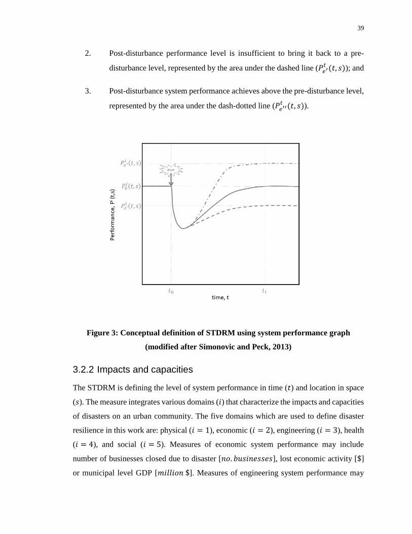
39
2. Post-disturbance performance level is insufficient to bring it back to a pre-
disturbance level, represented by the area under the dashed line (𝑃𝑒′𝑡 (𝑡, 𝑠)); and
3. Post-disturbance system performance achieves above the pre-disturbance level,
represented by the area under the dash-dotted line (𝑃𝑒′′𝑡 (𝑡, 𝑠)).
Figure 3: Conceptual definition of STDRM using system performance graph
(modified after Simonovic and Peck, 2013)
3.2.2 Impacts and capacities
The STDRM is defining the level of system performance in time (𝑡) and location in space
(𝑠). The measure integrates various domains (𝑖) that characterize the impacts and capacities
of disasters on an urban community. The five domains which are used to define disaster
resilience in this work are: physical (𝑖 = 1), economic (𝑖 = 2), engineering (𝑖 = 3), health
(𝑖 = 4), and social (𝑖 = 5). Measures of economic system performance may include
number of businesses closed due to disaster [𝑛𝑜. 𝑏𝑢𝑠𝑖𝑛𝑒𝑠𝑠𝑒𝑠], lost economic activity [$]
or municipal level GDP [𝑚𝑖𝑙𝑙𝑖𝑜𝑛 $]. Measures of engineering system performance may

40
include length of road [𝑘𝑚] inundated during a flood, the residential area [𝑘𝑚2] that is
inundated during a flood, or the damages [𝐶𝐴𝐷$] to municipal infrastructure. Measures of
health system performance may include the number of local emergency shelters
[𝑛𝑜. 𝑠ℎ𝑒𝑙𝑡𝑒𝑟𝑠], number of doctors available per capita [𝑛𝑜. 𝑑𝑜𝑐𝑡𝑜𝑟𝑠/𝑘𝑚2], or number of
people afflicted by disease [𝑛𝑜. 𝑝𝑒𝑜𝑝𝑙𝑒]. Measures of social system performance may
include the number of people who lose their homes in a flood [𝑛𝑜. 𝑝𝑒𝑜𝑝𝑙𝑒], amount of time
[𝑑𝑎𝑦𝑠] to receive insurance payments, or less tangible qualities such as the sense of
community [𝑑𝑚𝑛𝑙]. Each system performance indicator used in the quantification of
impacts may therefore be expressed in different units [$, 𝑑𝑎𝑦𝑠, 𝑝𝑒𝑜𝑝𝑙𝑒, 𝑒𝑡𝑐.], but can be
combined across domains for calculation of total resilience.
Changes in system performance, and subsequently resilience, can be represented
mathematically as:
𝜌𝑖(𝑡, 𝑠) = ∫ [𝑃0𝑖(𝑡, 𝑠) − 𝑃𝑖(𝑡, 𝑠)]𝑑𝑡
𝑡
𝑡0
𝑤ℎ𝑒𝑟𝑒 𝑡 ∈ [𝑡0, 𝑡𝑟]
(3.2)
Equation (3.2) will have the units of the selected domain impact indicator. Therefore, to
calculate an integral resilience measure across different domain impacts, the value of
𝜌𝑖(𝑡, 𝑠) is normalized as follows:
𝑟𝑖(𝑡, 𝑠) = 1 −∫ [𝑃0
𝑖(𝑡, 𝑠) − 𝑃𝑖(𝑡, 𝑠)]𝑑𝑡 𝑡
𝑡0
∫ 𝑃0𝑖(𝑡, 𝑠)𝑑𝑡
𝑡
𝑡0
(3.3)
This can be simplified to:
𝑟𝑖(𝑡, 𝑠) =∫ [𝑃𝑖(𝑡, 𝑠)]𝑑𝑡
𝑡
𝑡0
∫ 𝑃0𝑖(𝑡, 𝑠)
𝑡
𝑡0𝑑𝑡
(3.4)
When there is no degradation in performance, normalized resilience is one. When the
resilience value is zero, the performance of the system has been entirely and immediately
41
lost. In other words, when performance does not deteriorate due to disruption, 𝑃0𝑖(𝑡, 𝑠) =
𝑃𝑖(𝑡, 𝑠), the loss of resilience is zero, and the system is in the same state as at the beginning
of disruption. When all of system performance is lost, 𝑃𝑖(𝑡, 𝑠) = 0 and the loss of resilience
is at a maximum. As illustrated in Figure 4, performance of a system which is subject to a
disturbance (in this case a hazard event) at time 𝑡0, could cause significant damage such
that system performance is immediately reduced and takes time to recover (𝑡𝑟).
Disturbance to a system causes a reduction in system resilience from a value of one at 𝑡0
to some value 𝑟𝑖(𝑡1, 𝑠) at time 𝑡1 (Figure 5). Duration of the recovery is usually greater
than the duration of disturbance. Ideally, resilience should return to one at the end of the
recovery period and the faster the recovery (based on the slope of the recovery line), the
better. The system restores itself over time until 𝑡𝑟, the time at which it is completely
repaired, indicated by achieving pre-disaster performance level. In this example, additional
serviceability measures are incorporated into the repaired infrastructure which improves
system performance and achieves higher than pre-disturbance levels. If the systems’
performance is enhanced, it is possible that the time to recovery can be reduced and the
resilience value may surpass the pre-disturbance level. However, it is entirely possible that
if system performance is poor and improvement is slow, the recovery period will be longer
and in some cases the system may never return to the pre-disturbance level.
By time 𝑡𝑟, system performance has exceeded the original system performance level. When
the loss of system resilience (shaded area between 𝑡0 and 𝑡1) is equal to the recovery of
system resilience (shaded area between 𝑡1 and 𝑡𝑟), then the system resilience is equal to 1
at the end of the recovery period, 𝑡𝑟.
There are three potential outcomes of the resilience simulation:
1. Resilience returns to pre-disturbance level (𝑟𝑖 = 1) represented by the solid line
in Figure 5;
2. Resilience exceeds pre-disturbance level (𝑟𝑖 > 1) represented by the dash-
dotted line in Figure 5; or
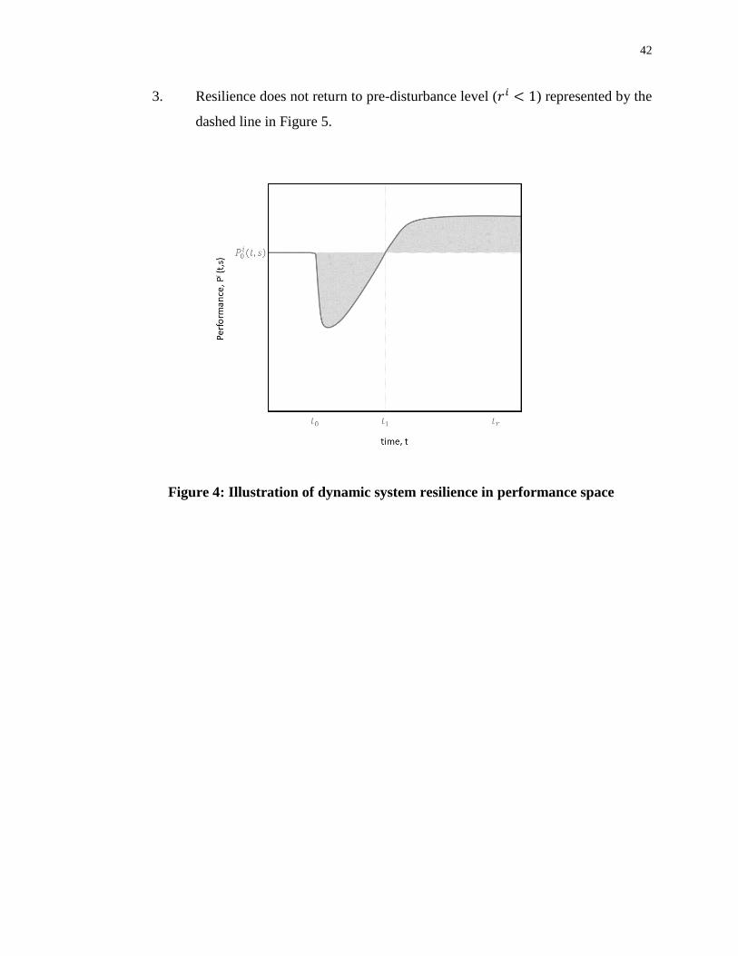
42
3. Resilience does not return to pre-disturbance level (𝑟𝑖 < 1) represented by the
dashed line in Figure 5.
Figure 4: Illustration of dynamic system resilience in performance space

43
Figure 5: Illustration of dynamic system resilience in resilience space demonstrating
examples of resilience which returns to pre-shock levels (solid line); exceeds pre-
shock levels (dash-dot line); and does not recover to pre-shock levels (dotted line)
One way of integrating various impacts is to consider the integral STDRM over all impacts
(𝑖), calculated as:
𝑅(𝑡, 𝑠) = {∏ 𝑟𝑖(𝑡, 𝑠)
𝑀
𝑖=1
}
1𝑀
𝑤ℎ𝑒𝑟𝑒 𝑀 𝑖𝑠 𝑡ℎ𝑒 𝑡𝑜𝑡𝑎𝑙 𝑛𝑢𝑚𝑏𝑒𝑟 𝑜𝑓 𝑖𝑚𝑝𝑎𝑐𝑡𝑠
(3.5)
Since the calculated value of 𝑅(𝑡, 𝑠) is dependent on time and location, the outcome of the
STDRM computation is a dynamic map that shows change of 𝑅(𝑡, 𝑠) in time and space
(Figure 6). This schematic presentation of the STDRM computational process illustrates
different resilience values in space, indicated by the shades of red colour. Spatial units of
the analysis are shown as grid cells for the simplicity of the concept illustration. The spatial
resolution for resilience analysis may require aggregation or disaggregation of indicators
selected for description of various impacts, (𝑖). This is, in part, driven by the availability

44
and resolution of resilience indicator data. For STDRM implementation in Canadian cities
the dissemination area (DA) is a useful spatial unit for analysis. This area is defined by
Statistics Canada (2018) as “a small, relatively stable geographic unit composed of one or
more adjacent dissemination blocks. It is the smallest standard geographic area for which
all census data are disseminated”. Any resilience indicator which relies on Statistics
Canada data is readily available in this form and allows easy integration with other DA-
level resilience data. Additional details pertaining to spatial resolution and scale of analysis
are contained in Section 3.3 describing the development of the Resilience Simulator Tool
(DRST).
Figure 6: Illustrative dynamic resilience map in time (t) and space (x,y) using
STDRM where the changing colours represent changes in resilience
3.2.3 Thresholds
Thresholds are important to the behaviour of systems and in defining and quantifying
disaster resilience. Thresholds are used to define the limits of a system, the safe operating

45
range for which a system will function as intended. Beyond these thresholds, a system may
function differently, or not at all. Operating outside of thresholds can initiate or break
critical feedback processes and can cause a system to operate under a different regime and
exhibit different, often undesirable, system behaviour. Thresholds may represent limits to
growth or tipping points of a system (Bennett et al., 2005). Walker and Salt (2012) suggest
there are four (4) types of threshold-related behaviours as follows (illustrated in Figure 7):
1. No threshold effect;
2. Step-change;
3. Alternate stable state; and
4. Irreversible change.
(a)
(b)
(c) (d)

46
Figure 7: Four types of threshold responses including (a) no response; (b) step-
change; (c) alternate stable state; and (d) irreversible change
(adapted from Walker and Salt, 2012)
Once a threshold is crossed, it’s possible that other system variables may also be influenced
and undergo significant changes. Thresholds in one disaster resilience domain may
influence thresholds in other domains. When a key threshold is crossed, it may also trigger
(or accelerate) the crossing of multiple other thresholds. This type of behaviour is what
often leads to cascading system failures.
Some thresholds are well understood, particularly in physical systems; for example, the
conversion of water to ice at a temperature of 0°C. However other thresholds – particularly
in social and health systems – are more difficult to identify and are not always well
understood. Moreover, threshold values are often not apparent until they have already been
crossed, which means they often go unnoticed until it’s too late. This poses a challenge to
defining reliable thresholds in a system model. The process often becomes iterative and, in
many instances, the identification of system thresholds is based on expert opinions and/or
previous experience.
To further add to the complexity of system behaviour, thresholds are not always fixed. That
is, it’s possible for certain thresholds to move (Walker and Salt, 2012). Changes in a system
can move a variable threshold up or down, thereby increasing or decreasing a systems safe

47
operating space (Figure 8). The shrinking or expansion of the safe operating space caused
by the movement of thresholds has an impact on system resilience (Bennett et al., 2005).
At any given time, it’s important to know how far away a system state is from a threshold
and how fast the variable is moving towards or away from the threshold. It’s therefore
important to know what defines the position of a threshold, and to determine whether it’s
possible for this threshold to move, in order to properly manage resilience.
Figure 8: Schematic example of a moving threshold
Not all systems or system variables possess thresholds, but it’s important to identify which
ones do. The quantification of disaster resilience as included in this research relies on key
thresholds to define domain (economic, engineering, health, and social) subsystem
responses to hazards. These thresholds come in the form of various system elements that
contribute to system behaviour and subsequently, to system performance. In fact, it’s
possible to have many relationships between controlling (x) and dependent (y) variables
within system elements that defines a system’s performance. However, it’s also possible
that thresholds be expressed as part of the description of system performance itself. In other

48
words, a threshold can be expressed in the units of the performance indicator [$, days,
people, etc.] and may be represented as a constant or function over time. The threshold acts
as an indicator of safe operating space and has implications on system resilience. A
system’s proximity to a performance threshold is governed by:
1. The initial state of the system (how close the system is to a threshold to begin
with); and
2. The rate at which the state of the system is approaching or receding from the
threshold (the redundancy and resourcefulness of the system).
This means that even if a system’s performance remains the same, the system’s
resilience can be increased (or decreased) by moving the threshold up or down within
the performance space. For example, Figure 9 shows two conceptual scenarios of a
system that has been shocked. The two scenarios have the same performance curve, the
only difference is that the threshold in Figure 9a is higher than in Figure 9b. Scenario
A has less safe operating space (i.e. the performance curve is closer to the threshold)
than Scenario B. Therefore, Scenario B should be categorized as having a higher
adaptive capacity – and higher resilience – than Scenario A, even though the impacts
(after disturbance) were the same.
(a)
(b)
Figure 9: Schematic of conceptual thresholds in performance space for (a) Scenario
A: higher threshold; and (b) Scenario B: lower threshold

49
The previous expression of resilience quantification in equations 3.2 and 3.3 did not
account for the potential influence of thresholds on system performance. So, systems which
have key thresholds (defined as constants) linked directly to system performance, may
therefore require a modified description of system resilience as follows:
𝜌𝑖(𝑡, 𝑠) = ∫ [𝑃0𝑖(𝑡, 𝑠) − 𝑃𝑖(𝑡, 𝑠) − 𝑃𝑇
𝑖 (𝑡, 𝑠)]𝑑𝑡 𝑡
𝑡0
𝑤ℎ𝑒𝑟𝑒 𝑡 ∈ [𝑡0, 𝑡𝑟]
(3.6)
Resilience with the inclusion of a threshold can therefore be defined as:
𝑟𝑖(𝑡, 𝑠) = 1 −∫ [𝑃0
𝑖(𝑡, 𝑠) − 𝑃𝑖(𝑡, 𝑠) − 𝑃𝑇𝑖 (𝑡, 𝑠)]𝑑𝑡
𝑡
𝑡0
∫ [𝑃0𝑖(𝑡, 𝑠) − 𝑃𝑇
𝑖(𝑡, 𝑠)]𝑑𝑡𝑡
𝑡0
(3.7)
Although it is likely that a threshold value may be specified as a constant, this general
expression leaves the opportunity to capture the impact of a threshold as a function.
Though in a more simplified form, it may still be represented as:
𝑟𝑖(𝑡, 𝑠) =∫ [𝑃𝑖(𝑡, 𝑠) − 𝑃𝑇
𝑖 (𝑡, 𝑠)]𝑑𝑡 𝑡
𝑡0
∫ [𝑃0𝑖(𝑡, 𝑠) − 𝑃𝑇
𝑖(𝑡, 𝑠)]𝑑𝑡𝑡
𝑡0
(3.8)
Though it may be useful to express a system in terms of thresholds, they do present
challenges in their practical implementation. Due to the inherent difficulties associated
with identifying the presence and magnitudes of thresholds, any subsystem or variable
identified as having thresholds may need to be iteratively incorporated in order to
properly describe the system.
3.3 Setting the Resilience Landscape: Focal Scale
The concept of scale is important in the definition and behaviour of complex systems and
plays an important role in disaster resilience modelling. There are various scales relevant
to disaster management including: governance, political, and decision-making scales;
information management and information dissemination scales; and geophysical
50
boundaries or geographic scales. At any one time, disaster management is occurring at
multiple scales across multiple systems. The complexity of disaster management
necessitates an understanding of important systems and the scales that they operate within.
An increased understanding of cross-scale relationships can enhance the coordination and
effectiveness of disaster management efforts.
All complex systems, and their dynamics, are scale dependent. It’s therefore important to
identify the “scale of interest” at an early stage of system description. The scale of interest
(the focal scale) for this research is the Regional scale (a collection of lower-tier
municipalities). Regions, (and cities) can be described as complex systems of systems
which operate over a large range of scales. Understanding what happens at one scale of the
system is important, but offers an incomplete story, as each scale of a system influences
another. For example, if considering scale from a bottom-up approach, individual people
influence neighbourhoods, which influence communities, which influence cities, which
influence a province or nation. The reverse is also true; nations can influence cities, and
cities influence communities, which influence neighbourhoods, which influence individual
people. Therefore, to appropriately understand a particular system is to acknowledge that
there are influences from other scales above (larger scale) and below (smaller, embedded
scale) the focal system scale that are constantly interacting (Figure 10). A system cannot
be appropriately managed by considering only one scale.
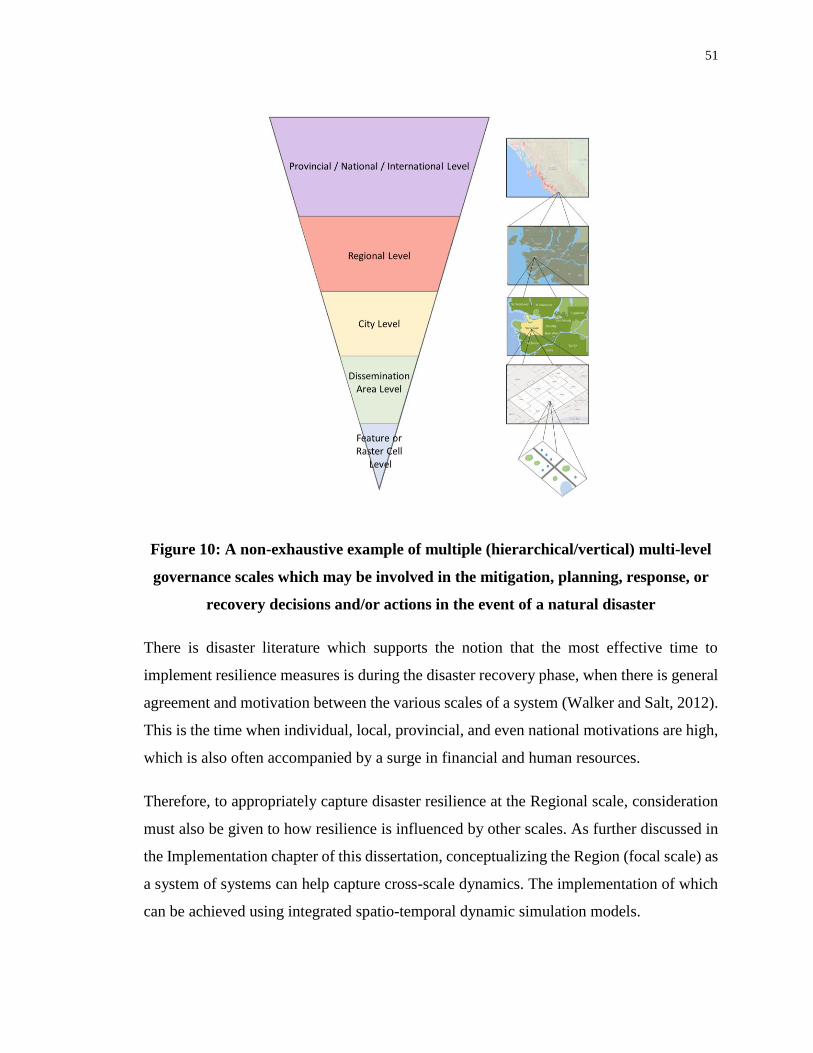
51
Figure 10: A non-exhaustive example of multiple (hierarchical/vertical) multi-level
governance scales which may be involved in the mitigation, planning, response, or
recovery decisions and/or actions in the event of a natural disaster
There is disaster literature which supports the notion that the most effective time to
implement resilience measures is during the disaster recovery phase, when there is general
agreement and motivation between the various scales of a system (Walker and Salt, 2012).
This is the time when individual, local, provincial, and even national motivations are high,
which is also often accompanied by a surge in financial and human resources.
Therefore, to appropriately capture disaster resilience at the Regional scale, consideration
must also be given to how resilience is influenced by other scales. As further discussed in
the Implementation chapter of this dissertation, conceptualizing the Region (focal scale) as
a system of systems can help capture cross-scale dynamics. The implementation of which
can be achieved using integrated spatio-temporal dynamic simulation models.

52
3.3.1 Characterizing Resilience: Interdisciplinary Resilience Domains
Quantification of disaster resilience requires characterization of resilient systems. It’s
necessary to define domains (systems) of interest and identify what contributes (or does
not contribute) to resilient system behaviour. Presently, there is still a gap in the universal
standardization of disaster resilience metrics and agreement even on qualitative measures
of disaster resilience remains a challenge. For this research, four (4) domains were
identified as significant to resilient city systems: economic, engineering, social, and health.
This decision was based on relevant resilience literature and driven by external (project-
based) factors.
The integrated resilience measure proposed in this research builds on the technical-
organizational-social-economic integration concept by Bruneau, et al. (2003) by
considering the resilience measure to be dynamic in both time and space. It also expands
on the approach of Bruneau, et al. (2003) by considering the spatial interactions between
physical, economic, engineering, health, and social domain responses to system disruptions
and provides a more comprehensive representation of disaster resilience.
53
Chapter 4
4 IMPLEMENTATION: AN INTEGRATED CITY SYSTEM
The methodology in this chapter is predicated on the recognition and acceptance of cities
as complex and dynamic systems made up of many smaller, multi-domain, integrated sub-
systems. These sub-systems interact with each other in any number of ways, across
multiple scales, and are managed and influenced by a number of various stakeholders
including engineers, architects, land developers, public safety managers, transportation
managers, council, committees, and community organizations.
The practice of trying to understand cities is not new. There are many professions and
disciplines that have looked at various resilience indices and metrics; some of which were
described in Chapter 2. With recent advances in the collection, organization, and
management of Big Data, there is motivation and capability to understand complex systems
and the methodological approach presented in this Chapter offers one way to represent the
complexities of city systems and quantify disaster resilience.
System dynamics simulation modelling can help inform disaster management policies and
decision making by providing insight into the underlying structure and behaviour of
complex real-world city systems. In this research, a city is modeled using system dynamics
as a network of interacting economic, engineering, health, and social subsystems. Everyday
basic functioning of a city was simulated to provide a baseline scenario for comparison,
and then this system was “shocked” by a climate change influenced hazard to estimate the
potential impacts in each city domain. Resilience concept was used as the primary means
of evaluating various adaptation options to help inform future disaster management
practice.
The proposed methodological approach to modelling and quantifying dynamic space-time
disaster resilience involves a systems approach. This chapter describes the implementation
of the resilience methodology. With reference to Figure 2, this chapter focuses on
implementation of dynamic disaster resilience quantification.
54
4.1 Implementation: Disaster Resilience Simulation Tool (DRST)
The basis for developing a DRST relies on the definition of a city as a sustainable network
of physical (constructed and natural) systems and human communities (social and
institutional) that possess the capacity to survive, cope, recover, learn, and transform from
disturbances by: (i) reducing failure probabilities; (ii) reducing consequences; (iii) reducing
time to recovery; and (iv) creating opportunity for development and innovation from
adverse impacts.
The DRST combines system dynamics simulation and spatial analysis to understand the
behaviour of complex city systems subject to climate change influenced disasters. This
approach was selected to capture the dynamic characteristics of disaster impacts and
disaster resilience behaviour of coastal cities. Adaptation scenarios are used to introduce
potential adaptation strategies into the resilience model, observe the effects on model
behavior, and identify areas where adaptation policy may be most effectively implemented.
These adaptation scenarios may also be used to modify physical hazard inputs (e.g. increase
in rainfall intensity) and simulate the impacts of multiple consecutive or concurrent
hazards. The remainder of this chapter will describe the basic temporal and spatial concepts
used to develop the DRST. The general implementation methodology is presented in Figure
11.

55
Figure 11: Generic implementation methodology

56
The quantitative resilience assessment calculation and methodology is implemented using
system dynamics (SD). SD is a computer simulation technique with foundations rooted in
the complex behaviour of dynamic, interdependent systems driven by feedbacks,
commonly used for the purpose of gaining insight into real-world system behavior
(Forrester, 1969). This approach was first introduced by Jay Forrester in the mid-1950s as
a framework for the conceptual representation as well as the quantitative modelling of
economic systems (Radzicki and Taylor, 1997). Since then, SD modelling has also been
applied to study environmental processes, water resource management (Khan et al., 2009;
Gastélumet al., 2010; Ahmad and Simonovic, 2000) and the energy resource domain. The
ultimate goal is to provide insight into real systems behaviour and act as a decision support
tool for stakeholders and policymakers.
“Disaster Resilience Simulation Tool” (DRST) is the name given to the Python script (and
associated input files) which integrates and automates the functionality of three software
programs:
1. ArcGIS, for spatial modelling;
2. Vensim, for temporal modelling; and
3. GAMS, for optimization modelling.
ArcGIS is used to display, analyze, and manage spatial data. The Python module ArcPy is
used to provide a flexible way to automate geoprocessing tasks and spatial analysis tools.
Vensim is used to model the connectivity and relationships between elements and to
simulate the temporal behavior of city systems over time. GAMS software is used to model
changes in the economy and subsequently, economic responses to disruptive shocks. The
DRST connects this software and automates the spatio-temporal simulation of complex
interactive processes within a city system. This integration makes the simulation process
more straightforward, computationally efficient, accurate, and transferable.
The DRST is composed of five interacting resilience domains: physical, social, economic,
engineering, and health. Each of these domains contributes to the calculation of disaster

57
resilience to estimate disaster impacts and identify opportunities for improvements. The
DRST is used to simulate the change in city resilience as a consequence of various
adaptation scenarios. A set of adaptation scenarios represents one simulation scenario and
provides one set of dynamic resilience maps and graphs. It is therefore possible to compare
simulation outputs (in the form of resilience) relative to each other, to evaluate the
performance of each adaptation option and create actionable items.
The DRST was developed for short term, event-based simulation to capture the more
immediate impacts of event-based short and medium duration climate hazards such as
flooding. This is captured in the physical domain of the DRST. This chapter provides a
description of each model domain (physical, economic, engineering, social, and health)
and presents resilience as framework for integration of impacts.
Water resources engineering practice needs to embrace the use of system dynamics
simulation as a modelling technique useful for the management of disasters. The DRST
uses system dynamics simulation modelling as a mechanism for dynamic resilience
calculation. Since resilience is calculated using a system dynamics simulation model, the
question of stationarity is left with the system inputs and not the system model. It’s an
effective approach for revealing temporal behavior of complex systems, such as cities.
Although there have been recent developments in expanding SD to include systems’ spatial
dependencies, most applications have been restricted to the simulation of diffusion
processes. Although SD research is trending in this direction, “the spatial dimension has
not received a great deal of attention in system dynamics modelling. An intensive literature
review showed that there are only a number of articles dealing with this subject” (Sanders
and Sanders, 2004, p9).
System dynamics simulation is a mathematical modelling technique which formalizes the
relationships between elements in a system. System [structure] refers to the patterns of
interactions between various system elements. Dynamics refers to the changes in these
patterns over time. Simulation involves the production of a system model, which is then
used to study the behaviour of the system in response to various stimuli. Thus, system
dynamics simulation links the dynamic behaviour of a system to its underlying structure
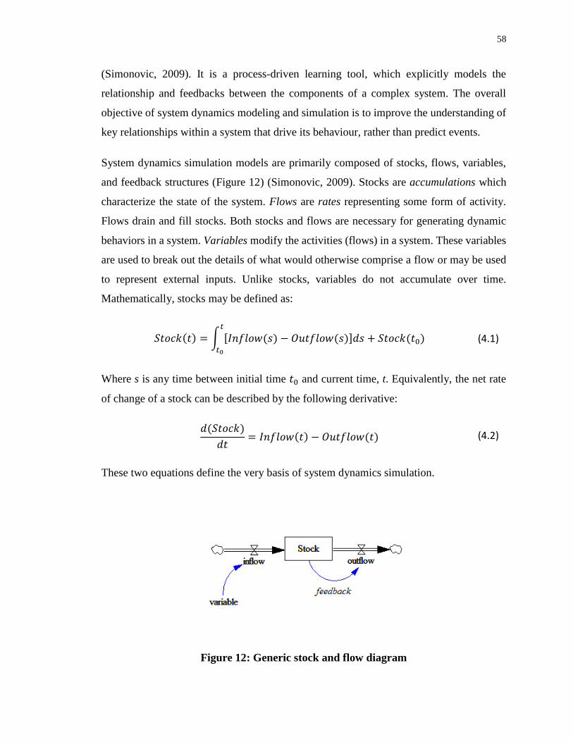
58
(Simonovic, 2009). It is a process-driven learning tool, which explicitly models the
relationship and feedbacks between the components of a complex system. The overall
objective of system dynamics modeling and simulation is to improve the understanding of
key relationships within a system that drive its behaviour, rather than predict events.
System dynamics simulation models are primarily composed of stocks, flows, variables,
and feedback structures (Figure 12) (Simonovic, 2009). Stocks are accumulations which
characterize the state of the system. Flows are rates representing some form of activity.
Flows drain and fill stocks. Both stocks and flows are necessary for generating dynamic
behaviors in a system. Variables modify the activities (flows) in a system. These variables
are used to break out the details of what would otherwise comprise a flow or may be used
to represent external inputs. Unlike stocks, variables do not accumulate over time.
Mathematically, stocks may be defined as:
𝑆𝑡𝑜𝑐𝑘(𝑡) = ∫ [𝐼𝑛𝑓𝑙𝑜𝑤(𝑠) − 𝑂𝑢𝑡𝑓𝑙𝑜𝑤(𝑠)]𝑑𝑠 + 𝑆𝑡𝑜𝑐𝑘(𝑡0)𝑡
𝑡0
(4.1)
Where s is any time between initial time 𝑡0 and current time, t. Equivalently, the net rate
of change of a stock can be described by the following derivative:
𝑑(𝑆𝑡𝑜𝑐𝑘)
𝑑𝑡= 𝐼𝑛𝑓𝑙𝑜𝑤(𝑡) − 𝑂𝑢𝑡𝑓𝑙𝑜𝑤(𝑡) (4.2)
These two equations define the very basis of system dynamics simulation.
Figure 12: Generic stock and flow diagram
59
Forrester (1990) presents a set of principles that helps to define, understand, and implement
system dynamics simulations as follows:
Principle 1: A feedback is a closed system
Principle 2: Every decision is made within a feedback loop
Principle 3: The feedback loop is the basic structural element of a system
Principle 4: A feedback loop consists of stocks and flows
Principle 5: Stocks are integrations
Principle 6: Stocks are changed only by flows
Principle 7: Stocks and flows are not distinguished by units of measure
Principle 8: No flow can be measured except as an average over a period of time
Principle 9: Flows depend only on stocks and constants
Principle 10: Stock and flow variables must alternate
Principle 11: Stocks completely describe the system conditions
Principle 12: A policy or flow equation recognizes a local goal towards which that decision
strives
These principles form the basis for system dynamics simulation and are the governing
principles which apply to the model developed in this work. In terms of methodology, the
system dynamics simulation approach presented in this dissertation is well-suited for
capturing the behaviour of complex city systems. It encourages holistic, “big-picture”
thinking that makes it appropriate for disaster management applications.
A critical component of modeling and understanding complex systems is through a
computer-based system dynamics simulation approach. Building a simulation model
requires the creation of a mathematical-based model that represents the related real-world
60
system that is being studied. Models of complex systems are often comprised of many
components and interactions and therefore computers and system dynamics simulation
software are typically used to facilitate the computations. Simulation models then form a
basis for experimental investigations. This proves particularly useful to the field of disaster
management where experimental investigations can take place in a simulation environment
without the associated risks, consequences, time, and expense of changing actual systems.
These simulation models can be used to assist decision makers and provide a set of tools
to evaluate the performance of various decisions and help them understand and learn within
complex environments.
4.1.1 System Dynamics Applications in Disaster Management
Although most of the system dynamics research in the past few decades has focused on
applications in social studies, economics, engineering, healthcare, environment, and the
military (Forrester, 2007), systems dynamics is gaining momentum in the field of disaster
management. There are examples of system dynamics applications to model problems
related to earthquakes (Xie and Rao, 2014; Ramezankhani and Najafiyazdi, 2006);
tornados; and flooding, among others. The system dynamics approach is widely applicable
to many problems because systems (and hazards) are prevalent across the globe. A systems
approach can help clarify the problem being studied, reveal complex and sometimes
counter-intuitive system behaviours, and test potential real-world solutions (Simonovic,
2009).
Ramezankhani and Najafiyazdi (2006) use a system dynamics model to simulate post-
disaster management in Iran following the Bam earthquake. The model included simulating
population, food supply, medical requirements and disease outbreaks, rescue teams, public
perception and media coverage, building destruction, and debris removal. Five strategies
(simulation scenarios) were tested to study the behaviour of model sectors and help answer
critical questions related to disaster response and determine which strategies may reduce
casualties. This simulation effort was valuable as part of post-disaster forensics, however,
the real benefits of system dynamics simulation is being able to estimate potential disaster
impacts before they happen in an effort to curb negative consequences. In addition, this
example of system dynamics disaster management simulation only considered the post-
61
disaster response phase of disaster management and did not consider other essential
components of disaster management such as mitigation, preparedness, or recovery. This
proposed research considers all phases of disaster management for a more holistic approach
to improve disaster management decision making strategies at all stages.
Somewhat similarly, Khyrina et al. (2012) and Kuznecova and Romagnoli (2014) consider
a more general system dynamics simulation approach to disaster management in the
context of emergency preparedness which offers a valuable, but limited, investigation into
potential disaster management solutions. Kuznecova and Romagnoli (2014) recognized
cities as complex dynamic systems comprised of many components and feedback loops
which necessitate a sophisticated understanding of city systems. The study links the
concepts of cities (as urban metabolism and dynamics) and urban disaster resilience, going
so far as to have produced a high-level causal loop diagram for urban resilience. The study
appears to be limited to environmental and energy impacts on resilience and does not offer
a quantification scheme for resilience assessment. The study does, however, identify a key
relationship between communication and disaster resilience which will be further explored
as part of this dissertation.
Since system dynamics lacks the explicit ability to capture the spatial dimension of
dynamic resilience, the DRST also incorporates Geographic Information Systems (GIS)
datasets and spatial analysis tools to capture both the temporal and spatial dynamics of
resilience. The combination has the potential to solve a wide variety of problems
(Grossman and Eberhardt, 1992). The groundwork for this integration was laid by
(Neuwirth et al., 2015) where a Python program was used to tightly couple SD software to
GIS. The approach provided the required capacities for handling bidirectional and
synchronized interactions of operations between SD and GIS.
4.2 Implementation: Data Collection
Our world is inherently complex, but by modelling systems and their interactions, it is
possible to learn something about the whole system that may not have been obvious within
the original system complexities. By implementing dynamic disaster resilience using
spatial and temporal modelling, it’s possible to layer multiple datasets together, exploring

62
the interactions one dataset may have on another and exploring their contributions to the
performance of the entire system. Spatial modelling and analysis can provide insight into
what things are happening, where they are happening, and even help explain why things
are happening. It can help provide solutions to data-intensive, large-scope spatial analyses
problems.
Spatial data is often displayed visually using maps. These maps include location,
topographical, and attribute data. Each feature on these maps has spatial information tied
to it; usually as latitudinal and longitudinal coordinates. Historically, this spatial
information was collected and displayed using hand drawn maps and tables. However,
nowadays spatial information and maps are available in digital format using Geographic
Information Systems (GIS). There are many useful examples of applications of GIS in
water resources including the areas of flood recovery mapping, hydrographic analysis, and
watershed protection. The resilience quantification framework and methodology presented
in this research uses spatial data, spatial analyses, and spatial mapping in hazard definition
and resilience assessment using GIS.
4.2.1 Implementation: Focal Scale and Geographic Scales in Spatial Resilience Modelling
The focal scale for resilience should be established early in the resilience assessment
process. The focal scale will drive resilience quantification and assessment, and be used to
identify key systems and their relationships. The selection of a focal scale will to some
degree also impact the data collection efforts. However, at an implementation level, there
are multiple contexts for use of scale in spatial resilience modelling. Three (3) of the most
important ones include:
1. Scale as it refers to the relative size of an object or space as compared to its real
size on Earth;
2. Scale as a resolution of data; and
3. Properties of data such as points, lines, or polygons.

63
For example, a small scale map on a computer screen may be 1:1,000,000 – or, one million
times smaller than its actual size on Earth. On the other hand, a scale of 1:1 would be a
very large scale representation – or, the same size on the screen as its actual size on Earth.
The type of data and its properties often determine the resolution.
Data is collected at various scales and resolutions using various tools. These are typically
not consistent between datasets, therefore one of the greatest challenges in spatial resilience
modelling is analyzing and harmonizing spatial data to assess its fitness for use in spatial
analysis. However, with sufficient pre-processing, the fact that spatial analysis can
incorporate data at various scales and resolutions is one of its main benefits.
Selecting the focal scale for analysis is important because an area’s boundaries will affect
the values within that area. There is no single “correct” scale, but there are “appropriate”
and “less appropriate” scales for resilience assessment. Selection of an appropriate scale is
driven by problem definition and the intended use of results of resilience assessment.
Perhaps most importantly, identifying a scale – whatever it may be – should be established
early on in the resilience assessment process.
Some boundaries are seemingly arbitrary and invisible; others are political, topologically
driven, or administrative. The criteria used to collect and represent spatial data and
boundaries may evolve over time. Since boundaries modify spatial data, spatial analyses
may require modification over time as different aggregation areas can modify the analyses
and subsequently the results. Results will be a function of the spatial units used for the
analysis making selection of scale important, especially since decision making and policies
are often based on boundaries and data that are aggregated by area. Clearly identifying the
focal scale can reduce the chances of misinterpreting resilience assessment results.
The representation of statistics (for Canadian Census) is provided at various resolutions of
census units (e.g. CMA, CT, DA, etc.). These data provide a snapshot in time for various
demographic and economic statistics across the country. These spatial units represent
various levels of data aggregation commonly used in thematic mapping. The DRST uses
data at various scales, but computes resilience at the DA level, but at the end of resilience
calculation, the resilience calculation is provided Regionally (focal scale).
64
The remainder of this section provides details related to spatial analysis tools used in
resilience calculations in the DRST.
4.2.2 Implementation: Spatial Analysis
Spatial analysis can help simplify complexities and solve geospatial problems. The results
of spatial analyses can help inform policies and disaster management decision making.
Spatial analysis relies on geographic data and the spatial relationships between data. It can
be as simple as analysis of location, but usually includes characteristics of those locations
and therefore requires knowledge of topography, geometric properties, and attribute data.
It becomes especially important in dynamic spatio-temporal modelling where connectivity,
adjacency, orientation, and containment are topological properties essential to properly
capture spatial dynamics. Therefore, spatial analysis is critical in resilience modelling in
the DRST.
It is important to select an appropriate spatial tool for the spatial relationship being
modeled. Many spatial analyses are driven by (or limited by) the availability and access to
high resolution spatial data. Similarly, the selection of tools used in a spatial analysis is
driven by both the research question and data availability. The DRST uses multiple forms
of spatial analysis toolsets in resilience quantification and assessment: extract, overlay,
proximity, and reclassify. Each toolset performs specific spatial analysis of feature or raster
data. A description of the tools implemented in the DRST is provided in Appendix A.
4.2.3 Implementation: Geographic Information Systems (GIS)
All spatial data can be mapped using a Geographic Information System (GIS). A GIS is a
collection of components: hardware, software, data, people, and protocols. The remainder
of this section focuses on the software aspect of a GIS, specifically as it relates to the
DRST.
GIS is a useful computer tool for representing, processing, graphically displaying, and
manipulating spatial data and preserving topology of spatial relationships. There are many
advantages to using GIS as a tool for building resilience: easily updateable databases;
intuitive graphical interface; statistical, mathematical and geometric tools available to
65
preform spatial calculations; combining numerical attributes in a spatial format; spatial
overlay capabilities; and the ability to handle multiple formats of data. Combining the
temporal modelling of SD with spatial information in GIS is able to produce a time series
of maps (dynamic mapping) of resilience. These maps can be used to target areas for
effective capacity building. Maps are especially useful tools for representing and
communicating the DRST results because they are visually interesting and spatial patterns
are easily identifiable.
Datasets are the primary inputs and outputs for analysis, operations, and tools in a GIS.
Before its use in GIS software, most data require significant pre-processing and quality
review. The DRST uses ESRI’s ArcGIS Desktop software (ESRI, 2011) for spatial data
management, analyses, and mapping. This software is typically used to manage and
represent large amounts of spatial data. However, the software also has the capacity to
perform real-time data retrieval and spatial analysis. ArcGIS organizes spatial analysis
tools in toolboxes. These toolboxes contain collections of data management and spatial
analysis functions to modify geographic data. The DRST accesses these toolboxes and their
tools to perform spatial analysis for resilience assessment.
Although ArcGIS provides a strong platform for spatial operations and visualization, the
program is largely criticized for its limitations in modelling temporal dynamics of complex
systems. Therefore, this research integrates ArcGIS with Vensim (Ventana Systems Inc.,
2009) capabilities to consider combined spatial and temporal modelling.
4.2.4 Implementation: Integrated spatio-temporal modelling
The DRST uses a dynamic-link library (DLL) to access the temporal simulation and spatial
analysis tools outside of SD modelling and GIS software. DLLs are modules which contain
code that permits sharing between programs. They are collections of coded functions that
can be called by other modules or applications. DLLs are unique in that they are only
loaded at run time when an executable file loads them, thus the DLL can be updated
independently without updating the executable itself. It is also possible for DLLs to be
linked to other libraries and DLLs, thereby initiating cascaded loading of DLL files.

66
The Python module ArcPy (ESRI, 2011) is used to perform geoprocessing outside of the
ArcGIS software. This module accesses multiple GIS DLL files and allows spatial tools to
be accessed outside of the ArcGIS software which provides integration with other software
for resilience modelling. The DRST combines ArcPy ArcGIS module (many .dll files) with
a Vensim DLL (vendll32.dll) to access tools and functions from outside the programs. This
allows the DRST to combine the temporal modelling and simulation capabilities of system
dynamics with the spatial modelling and analysis capabilities of a GIS. The DRST also
uses a DLL file to use the functionality of GAMS (GAMS Development Corporation,
1987) economic modelling software, which is discussed in future chapters. Combining
these tools together is the technical development of the DRST (Figure 13). The foundation
for this coupling is further described in a report Peck et al. (2014).
Figure 13: Technical implementation schematic for the DRST
In summary, the DRST uses multiple spatial datasets of various types, spatial reference,
and scale as input into resilience simulation. The DRST is a combined spatio-temporal
resilience modelling tool using temporal modelling capabilities of SD combined with
67
spatial analysis tools supported by a GIS to support disaster management decision making
processes.
4.3 Implementation: Systems Model
In the DRST, resilience is calculated for each of the model domains and then combined
into a dynamic integrated resilience measure. To quantify resilience, a set of resilience
indicator variables was identified for each of the five resilience model domains based on
first hand experiences, expert knowledge, scientific literature, industry standards, and data
availability. These indicators are from different domains and are characterized in different
units. Their relative changes over the course of a flood event are used to characterize
resilience in time and space.
Each of the domains is based on the same generic model structure (Figure 14). This
conceptual model structure contains input variables, impact variables, adaptation variables,
and resilience calculation variables. The main inputs into each domain of the model are
climate change factors, vulnerability factors, and hydrometeorological hazard.

68
Figure 14: Generic model structure for each domain (I-n)
Each of the domains (I-n) uses climate factors, vulnerability, and physical hazards exposure
as the main Inputs into resilience model simulation. Impacts elements consider the
variables from Inputs and simulate the resulting consequences on the system. These
impacts, however, are tempered by the capacity of the existing system to absorb, resist, and
quickly recover from, the impacts. This effect is captured by variables in Adaptive Capacity
elements of the model. The variables in Impacts and Capacities are then used in Resilience
Calculation. Although the actual system variables may vary depending on the
implementation of each resilience domain, in the most generic form, key stock (level)
variables may be expressed as:
𝐼𝑚𝑝𝑎𝑐𝑡𝑠 𝐼 − 𝑛 = ∫(𝑖𝑛𝑓𝑙𝑜𝑤 − 𝑜𝑢𝑡𝑓𝑙𝑜𝑤) (4.3)
69
𝑅𝐻𝑂 = ∫(𝑎𝑑𝑎𝑝𝑡𝑖𝑣𝑒 𝑐𝑎𝑝𝑎𝑐𝑖𝑡𝑦 − 𝑖𝑚𝑝𝑎𝑐𝑡𝑠) (4.4)
The flood Impacts (I-n) variable could be represented by resilience indictor variables from
multiple domains. These impacts can be categorized into four types: direct tangible (e.g.
damages due to contact with floodwaters), indirect tangible (e.g. business interruptions),
direct intangible (e.g. loss of life) and indirect intangible (e.g. psychological suffering)
(Bubeck and Kreibich, 2011). Ideally, each domain’s model (I-n) would capture an
estimate for all four types of impacts. However, not all domains may identify impacts for
all four types. Future work could consider expanding the number of flood impacts
considered in resilience assessment.
However, Figure 14 is more of a generic structure to guide the development of application-
specific implementations of resilience quantification. Its expression in Figure 14 is not
meant to encapsulate a complete representation of all specific elements that constitute
dynamic resilience but to guide the incorporation of key aspects into disaster resilience
assessment. Further details pertaining to this generic structure can be found in the report
by Peck and Simonovic (2013).
The remainder of this chapter describes one example of the main impacts from each domain
from Figure 14, driven by the hydrometeorological climate hazard (flooding) from the
physical domain. It starts by describing how climate change may influence flood hazards
and describes how the DRST incorporates these changes. Following which, the remainder
of this chapter describes the development and implementation of the impacts and adaptive
capacity measures (Figure 14) for the remaining four (economic, engineering, health, and
social) resilience model domains.
4.3.1 Physical Hazard Domain: Description
Extreme riverine flooding events are one of the most frequent and costly natural hazards
in the world (IPCC, 2012; Burn and Whitfield, 2016). This research is interested in
exploring the impacts and capacities of urban communities to adapt to these hazards now
70
and into the future. As such, this research focuses on climate change influenced flooding
as the primary physical hydrometeorological hazard in resilience assessment.
Coastal environments are hydrodynamically unique from inland hydrological
environments. Coastal stream networks have upstream freshwater flow like most other
riverine networks. However, the downstream end of the river network outlets at the ocean
which results in a portion of the downstream river network to be heavily influenced by tidal
patterns. The upstream river reaches are often characterized by sections of the stream
network which behave similarly to any other comparable river system. However, since the
main river channel outlets at the ocean, there are distinct differences in the behaviour of
the downstream ends of these river networks in terms of flow dynamics, flow properties,
and river geomorphology. The confluence of riverine and ocean gives rise to special
estuarine environments; the zone where mixing of fresh and salt water occurs. The
dynamics of estuary environments are more complex due to the variability in salt water
stratification and mixing, wave dynamics, and the heavy influence of tidal action
(Stenström, 2004; Guha and Lawrence, 2013). Although the DRST physical domain does
not explicitly consider all the unique properties of these environments, it does use tidal
action and sea levels as part of hazard definition. Future work is recommended to determine
the potential additional impacts that estuary dynamics and physical system plays in the role
of flooding and disaster resilience.
Traditional floodplain maps are derived through modelling techniques which apply
hydrologic and hydraulic modelling using historical physical data. The hydrologic model
converts rainfall to runoff taking into consideration land surface characteristics such as
vegetation, permeability, and soil. The runoff (discharge) is then used as input into a
hydraulic model which is used to estimate water surfaces along the river channel. These
water surface profiles are typically used to delineate the extent and depth of flooding in
floodplain maps. These maps represent flood prone areas and spatial data which form
essential support for disaster management. However, one of the shortcomings of traditional
flood modelling and floodplain mapping studies is the underlying assumption of
stationarity; that the climate, weather and runoff processes and patterns of the past will
operate the future (Shrubsole, et al., 2003). However, hydrologic impact assessments have

71
found that precipitation patterns are changing due to climate change, which impacts other
significant hydrological processes (Eum et al., 2010). Changes in precipitation have
propagating effects throughout the hydrological cycle and can influence the quality,
quantity, and timing of runoff volumes, runoff peaks, streamflows, inundation extents and
depths. This research attempts to address this gap by offering one approach to incorporate
climate change projections into the traditional process of flood hazard estimations and
floodplain mapping. Ultimately, these climate change influenced inundation mapping
projections serve as the primary input into the DRST.
4.3.2 Physical Hazard Domain: Implementation
To begin this unique climate change influenced hazard assessment, it was necessary to
estimate the potential effects that climate change will have on future extreme flood events.
Therefore, the methodology incorporates climate change projections with traditional
engineering simulations of physical phenomena to generate new, climate change
influenced hazards.
The physical hazard domain is the only domain which has a direct influence on all four of
the other model domains. The output generated from the physical domain of the DRST is
used as input into each of the other four resilience model domains (economic, engineering,
health, and social). The climate change influenced riverine flood hazard extents and depths
influence impact calculations in each of the DRST model domains. The physical hazard
domain produces a time series of climate change influenced flood inundation maps
generated from future climate change projections, river characteristics, and detailed spatio-
temporal data. The general process for incorporating climate change and deriving these
flood maps and data is described in the remainder of this section.
The process for generating the climate change influenced inundation maps for the physical
domain of the model is completed in a series of tasks (Figure 15), which follows common
inundation mapping techniques used by the US Army Corps of Engineers. However,
because the DRST is interested in the impacts of potential future flood disasters, the
methodology is modified by introducing climate change parameters to modify hydrologic
and hydraulic modelling and simulation inputs, thereby generating modified inundation
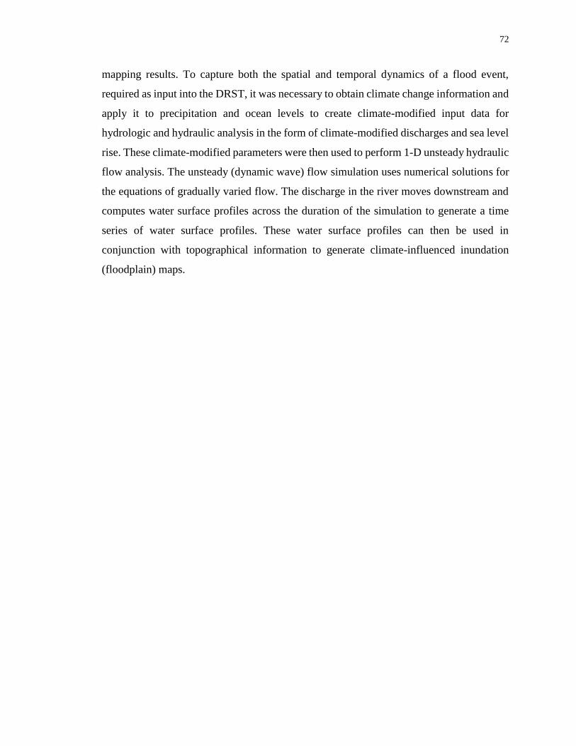
72
mapping results. To capture both the spatial and temporal dynamics of a flood event,
required as input into the DRST, it was necessary to obtain climate change information and
apply it to precipitation and ocean levels to create climate-modified input data for
hydrologic and hydraulic analysis in the form of climate-modified discharges and sea level
rise. These climate-modified parameters were then used to perform 1-D unsteady hydraulic
flow analysis. The unsteady (dynamic wave) flow simulation uses numerical solutions for
the equations of gradually varied flow. The discharge in the river moves downstream and
computes water surface profiles across the duration of the simulation to generate a time
series of water surface profiles. These water surface profiles can then be used in
conjunction with topographical information to generate climate-influenced inundation
(floodplain) maps.

73
Figure 15: Physical domain workflow diagram; tasks 4, 5, and 6 are completed for each unsteady flow simulation scenario

74
Defining Stream Characteristics
Automatic and semi-automatic characterization and description of hydrological features
(e.g. catchment delineation, slope profiling, flow direction, and stream network
identification) has become a popular technique among hydrological engineers, saving time
and often improving accuracy over traditional manual (hand-calculated) methods
(Steinfeld et al., 2013; Gopinath et al., 2014). The technological advancements, growth of
the GIS field, and improvement in high-resolution Digital Elevation Model (DEM) data
has enabled automatic extraction of important drainage network parameters useful for
hydrologic and hydraulic modelling (Lin et al., 2006). The characteristics of the extracted
stream network depend extensively on channel definition over the digital landscape and so
although the process has improved efficiency for hydraulic modelling and simulation, the
procedure is still data intensive and computationally demanding. This thesis suggests a
general digitization procedure similar to the one outlined in USACE’s HEC-GeoRAS
(2011) manual for extracting stream network features and characteristics for hydraulic
modelling (Figure 16). These features are required for use in hydrological and hydraulic
modelling and simulation to produce inundation maps for the DRST.

75
Figure 16: General river network digitization scheme (based on USACE (2011))
Climate Change Scenarios
Concentrations of GHGs such as carbon dioxide (CO2), methane (CH4), nitrous oxide
(N2O), chlorofluorocarbons (CFCs), and water vapor (H2O) in the atmosphere play a large
role in the warming of the planet, which in turn, plays a significant role in many
hydrological processes. The concentration of GHGs in the atmosphere varies over time and
space as a result of both natural (plant decomposition, volcanic eruptions, ocean
evaporation) and anthropogenic (burning of fossil fuels, deforestation, agricultural and
industrial activities) causes. According to some of the latest insights into projected GHG
emissions provided by the Intergovernmental Panel on Climate Change (IPCC) (Figure
17), CO2 emissions will likely continue to increase over at the next few decades. NASA’s
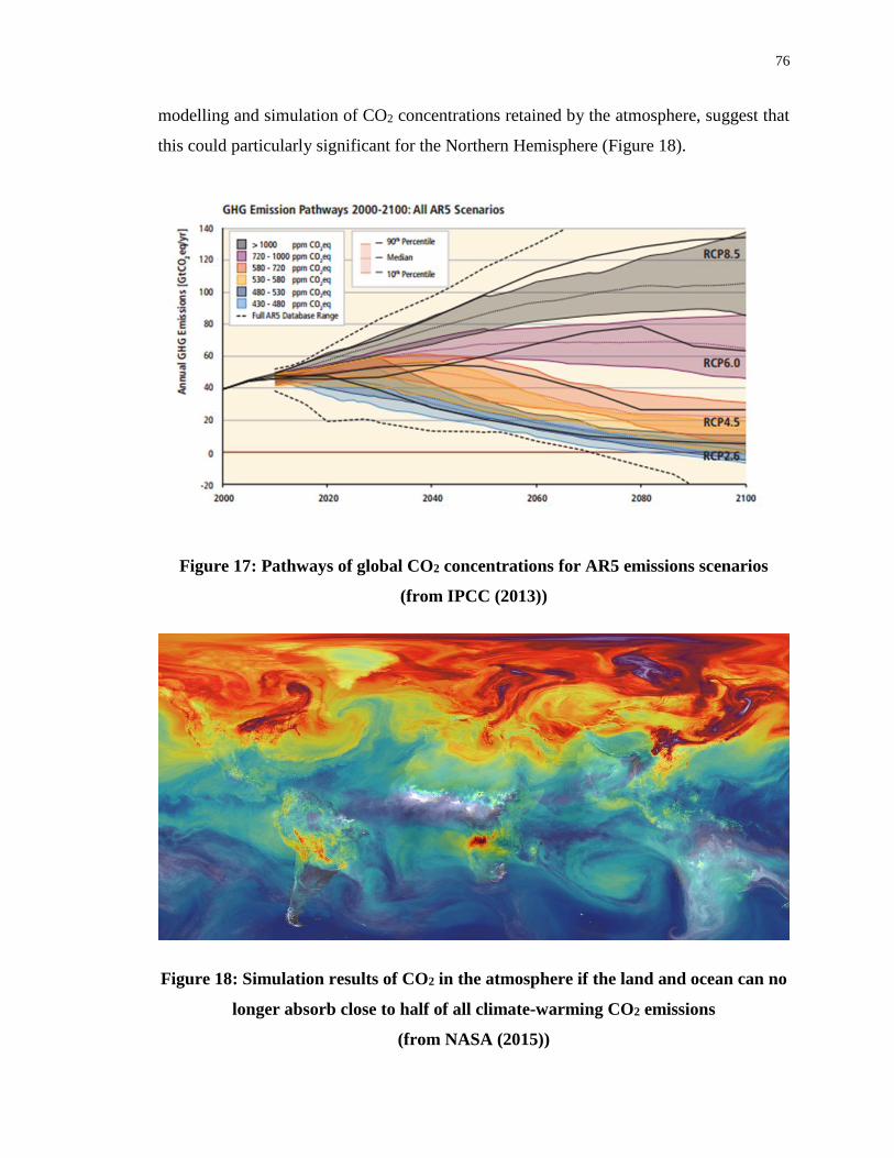
76
modelling and simulation of CO2 concentrations retained by the atmosphere, suggest that
this could particularly significant for the Northern Hemisphere (Figure 18).
Figure 17: Pathways of global CO2 concentrations for AR5 emissions scenarios
(from IPCC (2013))
Figure 18: Simulation results of CO2 in the atmosphere if the land and ocean can no
longer absorb close to half of all climate-warming CO2 emissions
(from NASA (2015))
77
The IPCC is one of the leading scientific bodies on climate change research and in 2007
they released their fourth Assessment Report (AR4) on the physics and science of climate
change. As part of this work, they developed four narrative emission scenarios representing
alterative futures, covering a wide range of the main driving forces which could be used as
a basis for climate change assessments. These emissions scenarios (A1B, A2, B1, and B2)
are outlined in an IPCC Special Report on Emissions Scenarios originally published in
2000 (IPCC, 2000). The A1 family of scenarios represent a future of rapid economic
growth, global population peak and decline, and introduction of efficient technologies; A2
family represents a heterogeneous world with regional economic growth, rapid and steady
population growth, and slow technological development; B1 family represents a future of
economic equity and sustainability, global population peak and decline, and clean
technologies; and finally B2 family of scenarios represent intermediate levels of economic
growth, slow and steady population growth, slow and diverse technologies. These
scenarios offer a range of climate changes in response to emissions, which the most
optimistic B1 scenario having projected a warming of by 1.8°C by 2100. Two of these
climate scenarios (A1B and B1) were used to generate climate change modified
streamflows in hydrologic modelling, which are subsequently used in hydraulic modelling
and flood inundation mapping inputs for the DRST.
The IPCC Fifth Assessment Report (AR5) was released in 2013 with updated emissions
scenarios called Representative Concentration Pathways (RCPs). There are four scenarios
(RCP2.6, RCP4.5, RCP6 and RCP8.5), each representing a different emissions scenario
future. RCP2.6 represents a mitigation scenario with low forcing; RCP4.5 and RCP6 are
stabilizing scenarios and RCP8.5 is the scenario with high GHG emissions (IPCC, 2013).
However, one thing remains common between the scenarios; total atmospheric CO2
concentrations are higher in 2100 than they are in present day.
The DRST uses gridded hydrologic modelling results driven by AR4 SRES A1B and B1
emissions scenarios as upstream boundary conditions in hydraulic modelling to capture the
potential changes in riverine flooding because of changing precipitation and runoff
volumes. The DRST uses sea level rise estimates generated using the AR5 RCP2.6 and

78
RCP8.5 emissions scenarios as downstream boundary conditions in hydraulic modelling to
capture potential changes in riverine flooding as a consequence of rising sea levels.
Sea Level Rise
Sea level rise (SLR) is a hazard threatening the world’s coastal cities. SLR can lead to more
severe storm surges, flooding, salt water intrusion and flood inundation resulting in severe
damage to coastal communities and environments. The two primary concerns related to
SLR, are the steady rise in the global mean sea level (GMSL) and the increased frequency
and magnitude of ocean wave events. SLR is caused by an increase in global ocean volume
caused primarily by two physical processes: thermal expansion of the ocean and the
melting of glaciers (IPCC 2013). These two phenomena are estimated to be responsible for
more than 80% of GMSL rise. The rate of GMSL has actually been rapidly increasing since
the 1900’s. The observed GMSL rise rate from 1901 – 1990 was 1.5 mm per year (IPCC
2013). This value then skyrocketed to over double the observed rate to 3.2 mm per year
from 1993 – 2010 and it is anticipated that SLR rates will continue to increase well into
the future, under all climate change scenarios (Figure 19) (IPCC 2013). There is inherently
high spatial variability in the magnitude of SLR estimations, due to factors such as oceanic
circulation patterns, salinity levels, and regional wind effects, but interestingly, it is very
likely that sea level will rise in more than 95% of the global ocean area, with 70% of
coastlines experiencing changes within 20% of the GMSL change (Figure 20) (IPCC
2013).

79
Figure 19: Projected SLR for RCP 2.6 (lower, blue projected line)
and RCP 8.5 (higher, red projected line) (IPCC, 2013)
Figure 20: Climate model ensemble mean relative sea level change (m) (between
1986-2005 and 2081-2100) for (a) RCP 2.6; and (b) RCP 8.5
(adapted from IPCC (2013))
(a)
(b)
80
The most common way to understand the potential impacts of SLR is to visualize potential
inundation extents by generating probabilistic or deterministic inundation maps (Gesch,
2009; Agam, 2014; Lentz, et al., 2016; NOAA, 2017). Deterministic methods use GMSL
rates and factors for regional considerations such as localized tidal data and vertical land
movements. Probabilistic methods use extreme value analysis in conjunction with local
tidal data to estimate the frequency of extreme SLR events. Deterministic SLR projections
were better suited for use in resilience assessment. However, SLR is a much slower
inundation phenomena than riverine flooding and so SLR inundation mapping in itself is
not appropriate as direct input into the DRST. Therefore, SLR is incorporated into the
physical domain of resilience assessment by specifying climate change influenced sea
levels as downstream boundary conditions in hydraulic modelling, thereby influencing the
flood inundation maps.
Hydrologic Modelling: Rainfall-runoff simulations
Hydrologic modelling uses a mathematical model to simulate hydrological processes in
watershed systems to estimate how watersheds respond to precipitation. In natural systems,
much of the water that falls as precipitation is returned to the atmosphere through
evaporation and transpiration processes. However, during storm events these processes are
limited and most of the rainfall becomes runoff. From there, runoff may pond on the
surface, infiltrate into the ground, or flow over land directly into a river channel.
Ultimately, river channel flow is the result of overland flows, precipitation which falls
directly into the channel, interflow (from vertical and horizontal movement of water in the
soil subsurface layers), and baseflow (from groundwater aquifers).
Hydrologic models can be stochastic or deterministic. Stochastic models are black box
systems which use mathematical and statistical concepts to relate rainfall to runoff.
Examples of stochastic modelling techniques include regression analysis and neural
networks. Deterministic hydrologic models represent real world physical processes and are
able to model more complex relationships between flows. Hydrologic models can be
simple (direct runoff) event-based models and can provide results in the form of peak flow
volumes or runoff hydrographs. Alternatively, models can be more complex (full moisture
81
accounting) continuous models which can provide results in the form of long duration
runoff records. The degree of hydrologic model complexity required to model these
processes is driven by the type engineering application and level of detail required in model
outputs. Some of the popular hydrological models include: variable infiltration capacity
(VIC) model developed by Liang et al. (1994) at the University of Washington; MIKESHE
developed by DHI Group; and soil water assessment tool (SWAT) developed by the Texas
Water Resources Institute at Texas A&M University. Although there is a variety of models
available, most traditional hydrologic modelling and simulation computations involves the
following constituents: state variables, parameters, boundary conditions, and initial
conditions. Basic data requirements often include: delineated watershed areas, site-specific
hydrological basin parameters (such as land use, soil cover, vegetation, and antecedent
moisture conditions, among others), simulation settings, and meteorological (precipitation,
wind, temperature) forcing data. Precipitation data may be specified as observed historical
precipitation data from rain gauges, frequency-based hypothetical rainfall events, or as
precipitation extremes (maxima).
This research used outputs from the VIC hydrologic model to generate runoff volumes
which are subsequently used in hydraulic modelling and simulation. The VIC model is a
macro semi-distributed hydrologic model originally created by Liang et al. (1994). It is a
gridded land surface model which uses parameter files, basin delineation, and a time series
of daily or sub-daily meteorological forcing data when coupled with statistically
downscaled GCM projections driven by future emissions scenarios (IPCC SRES climate
change scenarios A1B and B1) is able to simulate climate change influenced runoff.
(Figure 21). It was developed for use in coupled land surface model – global circulation
model (GCM) simulations. It’s based on a large grid cell size so it is intended for use is in
large (> 10,000 ha) sized basins to be coupled with GCMs to estimate stream flows and
atmospheric fluxes. The routing of streamflow within the channel is performed separately
from the land surface model using the model of Lohmann et al. (1998). Basic mathematical
relationships behind the VIC model are provided in Appendix B. Although this model was
selected primarily for its applicability to the case study area (Metro Vancouver / Fraser
River Basin) presented in Chapter 5, it may similarly be used to estimate climate change
influenced streamflows for other regions. There are a few of the benefits of the VIC model
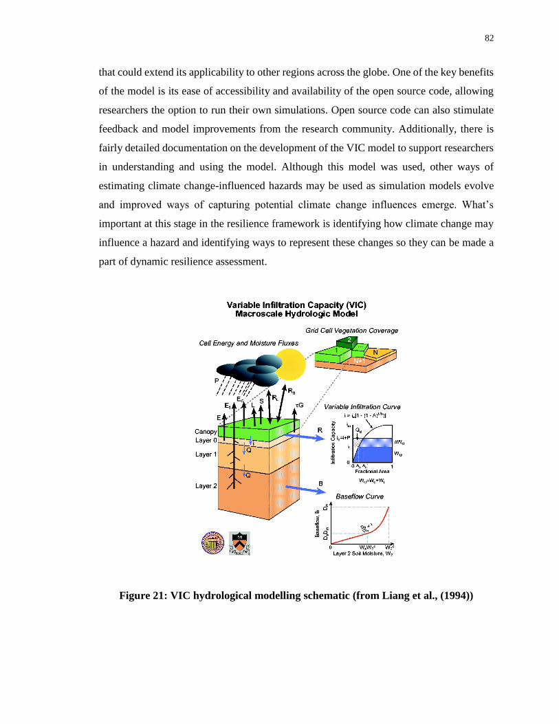
82
that could extend its applicability to other regions across the globe. One of the key benefits
of the model is its ease of accessibility and availability of the open source code, allowing
researchers the option to run their own simulations. Open source code can also stimulate
feedback and model improvements from the research community. Additionally, there is
fairly detailed documentation on the development of the VIC model to support researchers
in understanding and using the model. Although this model was used, other ways of
estimating climate change-influenced hazards may be used as simulation models evolve
and improved ways of capturing potential climate change influences emerge. What’s
important at this stage in the resilience framework is identifying how climate change may
influence a hazard and identifying ways to represent these changes so they can be made a
part of dynamic resilience assessment.
Figure 21: VIC hydrological modelling schematic (from Liang et al., (1994))
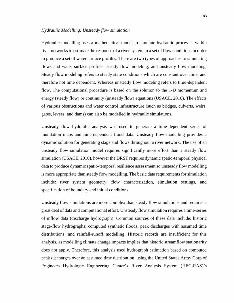
83
Hydraulic Modelling: Unsteady flow simulation
Hydraulic modelling uses a mathematical model to simulate hydraulic processes within
river networks to estimate the response of a river system to a set of flow conditions in order
to produce a set of water surface profiles. There are two types of approaches to simulating
flows and water surface profiles: steady flow modeling; and unsteady flow modeling.
Steady flow modeling refers to steady state conditions which are constant over time, and
therefore not time dependent. Whereas unsteady flow modeling refers to time-dependent
flow. The computational procedure is based on the solution to the 1-D momentum and
energy (steady flow) or continuity (unsteady flow) equations (USACE, 2010). The effects
of various obstructions and water control infrastructure (such as bridges, culverts, weirs,
gates, levees, and dams) can also be modelled in hydraulic simulations.
Unsteady flow hydraulic analysis was used to generate a time-dependent series of
inundation maps and time-dependent flood data. Unsteady flow modelling provides a
dynamic solution for generating stage and flows throughout a river network. The use of an
unsteady flow simulation model requires significantly more effort than a steady flow
simulation (USACE, 2010), however the DRST requires dynamic spatio-temporal physical
data to produce dynamic spatio-temporal resilience assessment so unsteady flow modelling
is more appropriate than steady flow modelling. The basic data requirements for simulation
include: river system geometry, flow characterization, simulation settings, and
specification of boundary and initial conditions.
Unsteady flow simulations are more complex than steady flow simulations and requires a
great deal of data and computational effort. Unsteady flow simulation requires a time-series
of inflow data (discharge hydrograph). Common sources of these data include: historic
stage-flow hydrographs; computed synthetic floods; peak discharges with assumed time
distributions; and rainfall-runoff modelling. Historic records are insufficient for this
analysis, as modelling climate change impacts implies that historic streamflow stationarity
does not apply. Therefore, this analysis used hydrograph estimation based on computed
peak discharges over an assumed time distribution, using the United States Army Corp of
Engineers Hydrologic Engineering Center’s River Analysis System (HEC-RAS)’s

84
interpolation routine. Unsteady, dynamic hydraulic modelling and simulation is governed
by the principles of the conservation of mass (continuity) and momentum (all variables are
described in Appendix C):
𝜕𝐴𝑡
𝜕𝑡+
𝜕𝑄
𝜕𝑥− 𝑞𝑖 = 0
(4.5)
𝜕𝑄
𝜕𝑡+
𝜕(𝑉𝑄)
𝜕𝑥+ 𝑔𝐴 (
𝜕𝑧
𝜕𝑥+ 𝑆𝑓) = 0
(4.6)
The program then performs calculations to establish flows and water levels in the cross
sectional profiles. Additional equations essential to the computational procedure are
provided in Appendix C.
Hydraulic Modelling: Boundary conditions
Hydraulic modelling of a river network requires the specification of boundary conditions
(BCs). There are upstream, interior, and downstream BCs. Upstream BCs are required for
all reaches (main channel and tributaries) which are not connected to other reaches.
Upstream BCs for unsteady flow analysis are specified as flow hydrographs (discharge vs.
time). Interior BCs are required to specify the relationship between reach connections.
They occur at junctions between tributaries and at places in the network where the flow
splits. These locations either apply the continuity of flow, or the continuity of stage
equations during hydraulic simulation. Downstream BCs are required at the end of all
reaches not connected to another reach. Unsteady flow downstream BCs may be specified
as either stage hydrographs, flow hydrographs, rating curves, or normal depths.
The climate change influenced streamflows are specified as flow hydrographs which were
introduced into the hydraulic modelling and simulation as upstream BCs (Figure 22). The
climate change influenced SLR projections are introduced into the model as downstream
boundary conditions (Figure 22). These BCs are specified at the edges of the model and
help define how the flow responds in the entire river system.

85
Figure 22: River schematic identifying locations which require the specification of
boundary conditions and where climate change is incorporated into the hydraulic
modelling process
Hydraulic Modelling: Output
Hydraulic simulation is time-dependent for dynamic unsteady flow. The unsteady HEC-
RAS computational procedure uses many of the same inputs and hydraulic calculations as
steady flow simulations, however the solution of the continuity and momentum equations
uses a unique solver (USACE, 2010). The unsteady flow simulation can be considered a
three-step process, and generates a collection of output files (Figure 23a) including a DSS
file containing a time-series of stage-time and flow-time plots. If the optional Post
Processor module is run, an output file is created containing detailed hydraulic results.
When the spatial water surface extents are exported from HEC-RAS to GIS and intersected
with spatial topographic data, it’s possible to generate a time-series of climate change
influenced inundation maps (Figure 23b). These are the maps used by the DRST to
determine domain impacts.

86
Figure 23: Schematic of physical domain output (a) generated from hydraulic
unsteady flow simulation; (b) when combined with spatial topographical
information to generate a time series of inundation maps
(adapted from USACE 2010)
4.3.3 Economic Domain: Description
Natural disasters can have severe and long-lasting economic consequences. Typically,
economic damage-and-loss assessments are conducted as part of post-disaster recovery
activities (European Union, United Nations Development Group, and The World Bank,
2013). These assessments are reactive measures intended to coordinate recovery efforts
and guide recovery planning. However, it would be valuable to be able to estimate these
damages and losses before an event occurs. Although progress has been made in modelling
the potential economic impacts of disasters, this area of research is still relatively new.
Gertz (2015) identifies three main approaches used to quantifying the economic impacts of
disasters: econometric techniques, input-output modelling, and computable general
equilibrium (CGE) models. Traditionally, input-output modelling was the most common
way to estimate the economic impacts of both man-made and natural disasters (Cochrane,
1974; Hallegatte, 2008; Rose, 2017). The popularity of this technique lies in both its ability
to reflect regional economic interdependencies and its methodological simplicity.
However, the rigidity and linearity of the input-output modelling approach which makes it
desirable also limits its effectiveness in adequately capturing the complex dynamic
87
behaviours of the economy in the event of a disaster. As such, CGE models have become
an increasingly popular way to model the impacts of disasters on the economy (Carrera et
al., 2015). CGE models are more flexible in their approach to modelling the elasticity of
economic supply and demand activities. Moreover, they are able to respond to price
changes, handle production processes, and incorporate goods substitutions into the
analysis, which better mimic real world disaster responses and more accurately captures
disaster dynamics. Therefore, the DRST uses an innovative, dynamic, regional CGE model
to estimate the economic impacts of a disaster.
4.3.3.1 Economic Domain: Implementation
The performance of the economy was identified as one of the indicators of economic
disaster resilience. Engineering resilience quantification was implemented in the DRST
considering the performance metric GDP as a proxy for the economy resilience indicator.
Therefore, economic system performance can be described as a function of the following:
𝑃𝑒𝑐𝑜𝑛𝑜𝑚𝑦𝑒𝑐𝑜𝑛𝑜𝑚𝑖𝑐 = 𝑓(𝐺𝐷𝑃)
The economic domain of the DRST is based on a multi-sector balanced growth CGE
model, used to capture the dynamic impacts of hydrometeorological disasters on the
regional economy. The CGE model used in the DRST was developed by Gertz (2015),
with minor modifications made by the author. The CGE model builds on work done by
(Hallegatte, 2008), but innovates by allowing the patterns and speed of recovery to be
determined endogenously. Herein, reference to the CGE model is assumed to be this
version in the DRST developed by (Gertz, 2015).
The CGE model is based on the optimization behavior of individual households and firms
(government) within a region. Each sector in the GCE model uses capital, labour, and
intermediate goods as inputs to production. The good produced by each sector is combined
with an imperfectly substitutable import to create an Armington good (Armington, 1969);
an elasticity substitution parameter for similar products produced in other countries. The
assumption is that imports are used as imperfect substitutes for domestic goods. The
Armington goods can then be consumed, invested, used as an intermediate in production,

88
or exported. The households and government then each optimize their stream of
consumption over time. A flood hazard is modeled as a shock to the capital stocks of
various industries. The economy slowly rebuilds the capital stock over time and converges
back to balanced growth. This optimization model is used to simulate the dynamic impacts
that a flood (a shock) may have on the economy (in the form of damages to capital stock).
Objective functions, decision variables, constraints, and parameters characterize an
optimization problem. A CGE model is an optimization model and can therefore be
described using conventional optimization modelling terms. The objective functions for
the DRST CGE optimization model includes the maximization of household and
government profits and utility; subject to model constraints. The representative household
chooses its stream of consumption and investment to maximize utility subject to budget
constraints. Mathematically, this process is described as:
max{𝑐𝑡,𝑖𝑡
𝑖}𝑡∈[0,∞)
∑ 𝛽𝑡𝑢(𝑐𝑡)
∞
𝑡=0
(4.7)
subject to
∑ [𝑝𝑡(1 + 𝜏𝐶)𝑐𝑡 + ∑ 𝑝𝑡𝐼𝑖
(1 + 𝜏𝐼)𝑖𝑡𝑖
𝑖
]
∞
𝑡=0
= ∑ ∑[(𝑤𝑡𝑖 − 𝜏𝐿)𝑙𝑡
𝑖 + (𝑅𝑡𝑖 − 𝜏𝐾)𝑘𝑡
𝑖]
𝑁
𝑖=1
∞
𝑡=0
(4.8)
𝑘𝑡+1𝑖 = (1 − 𝛿𝑖)𝑘𝑡
𝑖 + 𝑖𝑡𝑖 (4.9)
where 𝛽 is a discount factor, 𝑖𝑡𝑖 is sector-specific investments, and 𝑢(𝑐𝑡) is the household
utility function; where 𝑝𝑡 is the price of the composite consumption good, 𝑝𝑡𝐼𝑖
is the price
of the investment good, , 𝜏𝐶 is rate of sales tax on consumption goods, 𝜏𝐼 is rate of sales
tax on investment goods, 𝑤𝑡𝑖 is sector-specific wages, 𝜏𝐿 is tax rate on labour income, 𝜏𝐾
is tax rate on capital income 𝑅𝑡𝑖 is sector-specific return to capital; and where 𝑘𝑡
𝑖 is capital,
and 𝛿𝑖 is the depreciation rate. The government maximizes utility over its stream of
consumption subject to budget constraints. Mathematically, this is:

89
max{𝐺𝑡}𝑡∈[0,∞)
∑ 𝛽𝑡𝑣(𝐺𝑡)
∞
𝑡=0
(4.10)
subject to
∑ 𝑝𝑡𝐺𝐺𝑡 = ∑[𝑇𝑡
𝐿 + 𝑇𝑡𝐾 + 𝑇𝑡
𝑆𝑎𝑙𝑒𝑠]
∞
𝑡=0
∞
𝑡=0
(4.11)
where 𝛽 is a discount factor, and 𝑣(𝐺𝑡) is the government utility function; and where 𝑝𝑡𝐺 is
price of government consumption, 𝑇𝑡𝐿 is labour tax revenues, 𝑇𝑡
𝐾 is capital income taxes
revenues, and 𝑇𝑡𝑆𝑎𝑙𝑒𝑠 is sales tax revenues. The decision variables are prices and quantities
of the goods, capital, labour, and trade markets. All objective functions must satisfy model
constraints.
To determine share parameters for sector-specific production, the consumption bundles,
the investment goods, tax rates and trade shares, the CGE multi-sectoral model requires a
social accounting matrix (SAM). A SAM is a comprehensive economic accounting system
that captures all the transactions and transfers taking place between agents in a system over
a period of time. It provides details on sector-specific intermediate inputs, labour, capital,
taxes, and final demand (private consumption, government consumption, investment,
imports and exports). Unlike simple input-output models, a SAM is capable of modelling
inter-sectoral impacts by incorporating a complex household sector (Siddiqi and Salem,
2012). A well designed and disaggregated SAM provides insight about the structural
features and interdependencies of an economy. It represents a snapshot of the transactions
taking place during a period of time. The starting point for constructing a SAM is a regional
input-output table and a regional final demand table. Since the DRST was designed to
operate at the regional level, Gertz (2015) regionalized the provincial input-output and
demand tables using sectoral municipal-level employment data from Statistics Canada. The
SAM also requires a regional demand table which Gertz (2015) derived from detailed final
demand tables in industry accounts. In this way, a SAM was derived for use in the CGE
model.

90
The capital and labour sectors of the economics model are industry specific. Therefore, the
CGE model considers 20 different industry classifications (Table 3). Each building in the
spatial model is given one of these industry-specific classifications. The CGE model uses
this information, combined with flood hazard extent and depths to estimate the damages to
the capital stock in the form of damages (Figure 24). The maximum cumulative damages
by sector are sent from the spatial and engineering domains of the model to the CGE model
and then optimization operations are executed. In this way, it is possible to observe the
effects that a flood hazard will have on the economy.

91
Table 3: Industry-specific economic model sectors
Economic Code Economic Sector Description
B11 Agriculture, forestry, fishing, and hunting
B21 Mining, oil and gas extraction
B22 Utilities
B23 Construction
B31-B33 Manufacturing
B41 Wholesale trade
B44-B45 Retail trade
B48-B49 Transportation and warehousing
B51 Information and cultural industries
B52-B53, B55 Finance, insurance, and real estate
B54 Professional, scientific, and technical services
B56 Administrative and support
B61 Educational services (private)
B62 Healthcare and social assistance (private)
B71 Arts, entertainment, and recreation
B72 Accommodations and food services
B81 Other services (except public administration)
G61 Educational services (public)
G62 Healthcare and social assistance (public)
G91 Public administration
Figure 24: Schematic of spatial overlay and infrastructure attributes contributing to
economic CGE model
92
Additional details pertaining to CGE model development, including additional model
equations and assumptions can be found in Gertz (2015) with further refinement provided
in (Gertz et al., 2019).
Contrary to the other domains of the DRST, the economics model runs analysis at the city-
wide spatial scale. A shock, such as a flood, causes damage to industries that become
inundated, resulting in damages to the capital stock. The impact of the flood is reflected
in the regional GDP losses. Over time the capital stock rebuilds, and ultimately the solution
to optimization converges towards a balanced growth path. Since a regional economy does
not act independently of national or even global economies, there are additional parameters
within the economics model which include out-of-bounds influences such as importing and
exporting, and national GDP values, exogenous to the regional-level model.
The General Algebraic Modelling System (GAMS) software (GAMS Development
Corporation, 1987) was developed in partnership with the World Bank to provide a system
structure and programming language which maintains portability, generality, and ease of
implementation for mathematical optimization models. It supports multiple optimization
techniques including: linear programming; mixed-integer programming; non-linear
programming; constrained nonlinear systems; non-linear programming with discontinuous
derivatives; and quadratic constrained programs. The economic domain of the DRST uses
GAMS software for CGE modelling and optimizing complex economic activities during a
disaster. The generic organization of the economics domain GAMS program is provided
in Figure 25. The Municipal Level GDP and Loss by Sector optimization results are outputs
produced by the GAMS model. Municipal Level GDP growth rate is used as the
performance metric for the economy in Economic Resilience calculation in the DRST. A
more detailed description of the GAMS program and code is provided in Appendix D.

93
Figure 25: Schematic of the economics domain GAMS modelling and optimization;
this process is completed only once, at the end of the simulation
4.3.4 Engineering Domain: Description
Engineered infrastructure provides services to people and places within a city. Maintaining
the functionality and performance of this infrastructure often plays a critical role in disaster
management. Rarely are infrastructure systems independent of each other; typically, they
rely on each other to properly fulfill their intended purpose. These interdependencies
increase system complexities, which means well-intended decisions may result in
unforeseen adverse consequences. It is therefore important to consider these cross-
connections and interdependent system linkages.
Nan and Sansavini (2017) recently proposed a metric for resilience quantification of
interdependent infrastructures. They provide a multi-layer hybrid approach to capture
interrelationships between various infrastructure components as applied to an electric
power supply system. Each infrastructure (system) is broken down into its layers

94
(subsystems) and their components. Interactions occur both horizontally (within layers)
and vertically (across layers). The failure of any individual component could therefore
cause cascading failures which could affect the operations or functionality of the entire
system. The authors implement an Agent Based Model (ABM) to simulate the interactions
of agents (i.e. system components) [acting in accordance with pre-defined physical laws
and interaction rules] in the event of a disturbance – in their case study, a winter storm in
the central region of Switzerland. Three “resilience strategies” are compared to determine
which option may provide the best strategy for restoring power to pre-disaster levels. This
application is suitable for individual infrastructure resilience assessment; however, it
would be very complex to model using ABM across multiple infrastructure types and it
does not provide a substantial enough foundation for incorporating non-infrastructure-type
systems into resilience assessment. The DRST can estimate physical damages to school
buildings and contents under various flooding conditions.
4.3.5 Engineering Domain: Implementation
Building stock was identified as one (of many) indicators of engineering disaster resilience.
Engineering resilience quantification was implemented in the DRST considering the
performance metric structural and content damages as a proxy for the building stock
resilience indicator. Therefore, engineering system performance can be described as a
function of the following:
𝑃𝑏𝑙𝑑𝑔 𝑠𝑡𝑜𝑐𝑘𝑒𝑛𝑔𝑖𝑛𝑒𝑒𝑟𝑖𝑛𝑔
= 𝑓(𝑤𝑎𝑡𝑒𝑟 𝑑𝑒𝑝𝑡ℎ, 𝑏𝑢𝑖𝑙𝑑𝑖𝑛𝑔 𝑡𝑦𝑝𝑒, 𝑣𝑎𝑙𝑢𝑒 𝑜𝑓 𝑠𝑡𝑟𝑢𝑐𝑡𝑢𝑟𝑒, 𝑣𝑎𝑙𝑢𝑒 𝑜𝑓 𝑐𝑜𝑛𝑡𝑒𝑛𝑡𝑠,
𝑓𝑙𝑜𝑜𝑑 𝑝𝑟𝑜𝑜𝑓𝑖𝑛𝑔, 𝑟𝑒𝑐𝑜𝑛𝑠𝑡𝑟𝑢𝑐𝑡𝑖𝑜𝑛 𝑟𝑎𝑡𝑒)
The amount of damage directly depends on the depth of water in the area and therefore,
the performance of this system is highly spatially dependent. When a disturbance occurs
(such as a hazard event), it’s possible that buildings get damaged by floodwaters and the
building stock becomes impacted. As flood waters encroach on an area, the depth of water
increases. As the depth of water increases, inundated infrastructure sustains additional
damages. Once the building is no longer flooded, it’s possible for recovery actions to begin
and the building begin repairs.
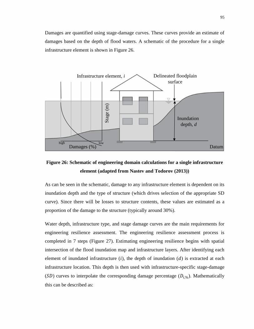
95
Damages are quantified using stage-damage curves. These curves provide an estimate of
damages based on the depth of flood waters. A schematic of the procedure for a single
infrastructure element is shown in Figure 26.
Figure 26: Schematic of engineering domain calculations for a single infrastructure
element (adapted from Nastev and Todorov (2013))
As can be seen in the schematic, damage to any infrastructure element is dependent on its
inundation depth and the type of structure (which drives selection of the appropriate SD
curve). Since there will be losses to structure contents, these values are estimated as a
proportion of the damage to the structure (typically around 30%).
Water depth, infrastructure type, and stage damage curves are the main requirements for
engineering resilience assessment. The engineering resilience assessment process is
completed in 7 steps (Figure 27). Estimating engineering resilience begins with spatial
intersection of the flood inundation map and infrastructure layers. After identifying each
element of inundated infrastructure (𝑖), the depth of inundation (𝑑) is extracted at each
infrastructure location. This depth is then used with infrastructure-specific stage-damage
(𝑆𝐷) curves to interpolate the corresponding damage percentage (𝐷𝑖,%). Mathematically
this can be described as:
Delineated floodplain
surface
Inundation
depth, d
Datum
Infrastructure element, i
Damages (%)
Sta
ge
(m)
low high

96
𝐷𝑖,% = 𝑓(𝑑𝑖, 𝑡𝑦𝑝𝑒) (4.12)
The damage percentage (𝐷𝑖,%) is then multiplied by the reconstruction value (𝑉𝑖,$) of the
infrastructure to obtain a dollar damage value (𝐷𝑖,$). Mathematically, this is simply given
by:
𝐷𝑖,$ = 𝐷𝑖,% × 𝑉𝑖,$ (4.13)
This process is repeated for every infrastructure element and then all of the damage values
are summed together for a total estimated damage value (𝐷𝑇,$).
(𝐷𝑇,$)𝑡 = ∑(𝐷𝑖,$)𝑡
𝑖
𝑡=0
(4.14)
This entire process is repeated for each time step. The damage at each time step (𝐷𝑇,$)𝑡 is
sent to engineering resilience calculations. The maximum summed damage value (𝐷𝑇𝑚𝑎𝑥,$)
is sent to the economic domain for use in economic resilience calculations.
𝐷𝑇𝑚𝑎𝑥,$ = max ((𝐷𝑇,$)𝑡) (4.15)
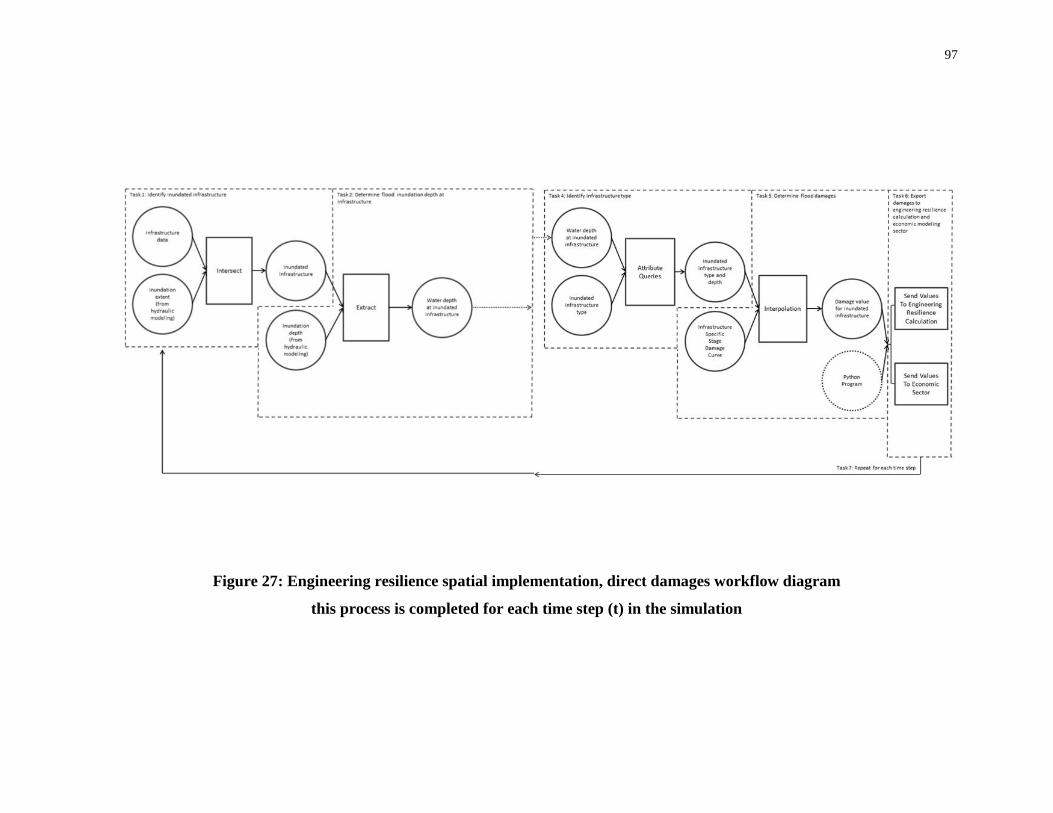
97
Figure 27: Engineering resilience spatial implementation, direct damages workflow diagram
this process is completed for each time step (t) in the simulation

98
Since this process involves the use of spatial data, engineering resilience value will also be
spatially (and temporally) dynamic. At each time step, engineering resilience values are
aggregated up to the DA level, to achieve meaningful and compatible spatial resilience
results.
4.3.6 Health Domain: Description
Public health and wellbeing are inextricably linked to climate change (Patz et al., 2014). It
is therefore important to identify where the most climate hazard vulnerable communities
are and what reprioritization of health resources may be needed to help address future
health impacts. These resources may include improved disaster prevention, better
communication systems, quicker disaster response, or even stronger food and water
security. Intentional design in the public health domain is needed to build more resilient
health systems for the future.
Traditional health disciplines include medical (physical) health, behavioral health, and
social services. Although all three disciplines are important for comprehensive health
management and health resilience, the DRST considers only medical health in resilience
assessment. This choice was driven by available data and expertise in the medical field.
Therefore, the remainder of this section focuses on health resilience in the medical
(physical) health context.
Public health impacts due to natural disasters are inherently difficult to predict. Human
health is a complex phenomenon and the relationship between climate change and the
impacts it will have on human health is even more complex. This prediction is made even
more difficult by the challenging spatial and temporal dynamic characteristics of diverse
types of diseases. Data collection is difficult because diseases are not always reported nor
diagnosed correctly. This difficulty is exacerbated by data collection methods which are
dependent on both the human and financial resources of individual institutions. To
complicate issues, where data are collected, records are often protected by patient
confidentiality which limits the accessibility to health data.
99
Research suggests that public health capacities and consequences vary more by severity of
the disaster than the type of hazard (FEMA, 1996; Frumkin, 2010), although geophysical
disasters usually cause a greater number of injuries than meteorological disasters. The
DRST simulates the impacts due to flood events of various magnitudes, which is consistent
with these findings.
Injuries
Across all types of hazards, injuries are the primary cause of death (Luther, 2008; Luther,
2011); and drowning is the number one cause of death during a flood hazard (Malilay et
al., 1997; WHO, 2018). Possible types of injuries during a disaster include: electrocutions,
puncture wounds, falls, and carbon monoxide poisoning. Most of these injuries occur in
the response and recovery phases of a disaster when contact with floodwaters and debris is
highest. All sorts of debris can be carried by floodwaters, and when people come into
contact with this debris, it can impact their health. Intermixed debris from the hurricane
Katrina flood event included: municipal solid waste, vegetation, construction waste,
asbestos, hazardous waste, white goods (such as refrigerators, stoves, etc.), electronic
waste, and vehicles (Luther, 2008). This debris can cause serious injuries and propagate
the spread of communicable diseases.
Diseases: Infectious Communicable
Infectious diseases are caused by microorganisms. Infectious diseases most commonly
observed after a disaster include: acute respiratory infections, malaria, cholera, typhoid,
hepatitis, measles and meningitis. However, many of the most serious infectious diseases
are not commonly observed in North America. Malaria is a potentially life-threatening
disease caused by parasites, transmitted through the bite of female mosquitoes. It’s most
prevalent in sub-Saharan Africa, South-East Asia, Latin America, and the Middle East.
Cholera is an acute infection of the intestines caused by the bacteria Vibrio cholerae found
in the feces of infected people. It is commonly transmitted through consuming
contaminated food or water. Cholera is not a concern in Canada, but regions with
inadequate sanitation, poor hygiene, and overcrowding are at higher risk for infection.
Cholera is a health problem in many developing countries in parts of Africa, Asia, Central
100
and South America. In the Canadian context, measles and hepatitis do not have high
prevalence in the general population due to vaccinations administered to children at a
young age. However, children who have yet to receive the vaccination at the time of a
disaster are more vulnerable to experiencing negative health impacts. There’s also been
reported links between malnutrition and infectious diseases. In cases of prolonged post-
disaster food shortages, clinical malnutrition is a significant contributor to cause of death
(Watson et al., 2007). Flood waters can contain Campylobacter, Giardia, Cryptosporidium,
noroviruses, and enteroviruses associated with gastrointestinal illnesses caused by flood-
induced sewage overflows (Patz et al., 2014). Meta-analysis of global waterborne
communicable disease outbreaks have shown Vibrio and Leptospira were the pathogens
most often cited (Cann et al., 2013).
Those infectious diseases which can be transmitted from one source to another through
bacterial or viral organisms can be classified as communicable diseases (Heymann, 2016).
Meteorological disasters are only rarely associated with epidemics of communicable
disease (Keim, 2008), though many of the disaster-related disease deaths occur in displaced
populations, likely due to high-density shelter conditions and high incidence of person-to-
person transmissions. The displacement of populations (e.g. evacuations) is problematic
for the spread of communicable diseases, particularly in developing countries where there
are pre-existing conditions which contribute to the transmission of communicable diseases.
Types of communicable diseases include: water-borne, respiratory, mosquito-borne, and
rodent-borne. Sources of these diseases include: the built environment, freshwater
organisms, and ocean water organisms. Common modes of transmission of infectious
diseases include person-to-person, feco-oral, and vector-borne. Particular post-disaster
conditions may influence the person-to-person and feco-oral transmission of infectious
diseases post-disaster including: population characteristics, environmental conditions,
endemic organisms, pre-hazard condition of the public health system, and type, duration,
and magnitude of the hazard event. Furthermore, changes in the climate can influence the
transmission of vector-borne diseases through multiple mechanisms including:
Geographic shifts in the presence of vector-borne diseases;

101
Rates of development, survival, and reproduction; and
Increased biting and prevalence of infection.
The potential impacts of disasters on the spread of infectious diseases include: degradation
of water quality; population displacement and subsequent population shelter densities; poor
sanitation; increased sewage overflows; disruption of health services; decreased access to
public healthcare facilities; and loss of major lifeline utilities.
Wet, bog-like post-disaster conditions create environments that are favourable for disease
carrying insects (mosquitos carrying Malaria and Leptospirosis) and rodents (carrying
vector-borne disease strains) (Watson et al., 2007). To reduce the spread of these diseases,
it is good to reduce the favourable environment by increasing drainage (to reduce stagnant
water), debris and garbage removal, improve sanitation, practice safe food storage and
handling, and select dry shelter regions. In addition, improved infrastructure management
and proper infrastructure design can reduce the number of sanitary overflow events,
thereby reducing the spread of waterborne diseases.
Diseases: Non-communicable
There are also non-communicable diseases associated with the impacts of disasters.
However, these types of diseases are more difficult to track and specific disaster-related
impacts are particularly difficult to assess as they often go unreported or are diagnosed as
aggravations of pre-existing diseases and not necessarily associated as a consequence of
the disaster. Non-communicable diseases include: diabetes, neuropsychiatric
(schizophrenia), cardiovascular (rheumatic heart, hypertensive cardiac), respiratory
(asthma), and digestive (cirrhosis).
Other public health issues
Other post-disaster public health-related issues include: pollution (Zelenakova et al., 2016),
malnutrition (Datar et al., 2011; Global Nuitrition Cluster, 2008), mental health and trauma
disorders (Goldmann and Galea, 2014), and epidemics (rapid spread of infectious
communicable diseases). The detailed impacts that flood disasters have on human physical
102
and mental health are still not well understood (Chemtob et al., 2002), but qualitative
evidence suggests that at an individual level, full recovery may take many years to achieve
and financial, emotional, and mental costs related to health impacts may persist well into
the future.
In summary, the overall risk of communicable disease outbreaks after natural disasters is
relatively low, particularly when there is no substantial population displacement
(evacuation). They are more likely to occur in in displaced populations that struggle to
provide basic needs such as clean water, sanitation, and primary healthcare services
(Watson et al., 2007). Disaster-related deaths are overwhelmingly caused by the initial
traumatic (psychological and physical) impacts of the event (Watson et al., 2007) however
drowning, and other more immediate flood-related causes of death were not explored as
part of this work. Not only because these incidents are difficult to predict, but also because
flood-related deaths by drowning are relatively uncommon in a Canadian context. Instead,
the focus of health impacts was on treating people with injuries and/or continuing to
provide traditional health care services to the community in the event of a disaster.
Therefore, the implementation of the health domain focuses on restoration of access to
primary care facilities in the wake of a disaster.
4.3.7 Health Domain: Implementation
It is apparent that there is high spatial and temporal variability in health impacts since each
disease is active in different parts of the world and each has its own symptoms, onset time,
and latency period. This makes diseases inherently difficult to monitor, track, and treat.
During a disaster, it is particularly important to treat the injured and maintain adequate
healthcare function. Therefore, access to healthcare facilities was identified as one (of
many) indicators of health domain disaster resilience. Health resilience quantification was
implemented in the DRST considering the performance metric cost distance as a proxy for
the resilience indicator access to healthcare facilities. Access to healthcare facilities during
a non-flooding situation is dependent on road type, local traffic, and road network
connectivity. At the fundamental level, access to healthcare facilities during a flood is due
to the same factors, which are then influenced by the extent and depth of flooding across
the road network. This, in turn, is driven by the magnitude of the flood event and any

103
structural and non-structural measures in place to protect the road network. For the research
presented in this dissertation, health system performance was described as a function of the
following:
𝑃𝑎𝑐𝑐𝑒𝑠𝑠 𝑡𝑜 ℎ𝑒𝑎𝑙𝑡ℎ 𝑐𝑎𝑟𝑒 𝑓𝑎𝑐𝑖𝑙𝑖𝑡𝑖𝑒𝑠ℎ𝑒𝑎𝑙𝑡ℎ =
𝑓(𝑑𝑖𝑠𝑡𝑎𝑛𝑐𝑒 𝑡𝑜 𝑓𝑎𝑐𝑖𝑙𝑖𝑡𝑖𝑒𝑠, 𝑟𝑜𝑎𝑑 𝑡𝑦𝑝𝑒, 𝑟𝑜𝑎𝑑 𝑠𝑢𝑟𝑓𝑎𝑐𝑒, 𝑟𝑜𝑎𝑑 𝑎𝑐𝑐𝑒𝑠𝑠𝑖𝑏𝑖𝑙𝑖𝑡𝑦)
Since the provision of health services relies on the availability of roads (i.e. roads that are
safe to drive), the performance of this system is contingent on the road network and its
degree of flooding:
𝑟𝑜𝑎𝑑 𝑎𝑣𝑎𝑖𝑙𝑎𝑏𝑖𝑙𝑖𝑡𝑦 = 𝑓(𝑓𝑙𝑜𝑜𝑑 𝑑𝑒𝑝𝑡ℎ)
When a disturbance occurs (such as a hazard event), it’s possible that the provision of
emergency services is disrupted and access to healthcare facilities is disrupted when a road
becomes flooded and is no longer accessible.
The DRST uses this principle and spatial analysis tools to calculate a cost-distance metric
to public healthcare facilities at each time step during the simulation. This analysis
implements an algorithm which combines a cost-surface profile, flood inundation extent,
and water depth to calculate a cost-distance surface from public healthcare facilities to
every point in space. Essentially, this is a raster-based algorithm which assigns a penalty
factor to inundated roads; and the higher the depth of flooding, the greater the penalty (or
“cost”) would be to take that path to the hospital. The cost-distance algorithm determines
the shortest weighted distance from each cell to the nearest “source” (hospital) location.
Therefore, the output from this metric is a raster surface of cost units, not geographic
distances.
The cost-distance algorithm requires an input source raster file (in this instance, it would
be a raster dataset of hospital locations) and a single input cost-surface raster file (in this
instance, an aggregate cost-surface raster created from combining multiple cost raster
datasets (such as the road network combined with an inundation map). The source raster
file is a raster file representing the location of hospitals. The cost-surface raster file is a

104
raster file which is an aggregate-cost of all the input cost-surface raster files (road lanes;
road type; road surface; and flood depth). The following outlines the cost-distance
algorithm implemented in the calculation of health resilience in the DRST. This step-by-
step description of the process is supported by Figure 28.
Step 1: The algorithm assigns a value of zero (0) to the source (hospital) cells
Step 2: The neighbouring cells to the source cells are activated.
Step 3: The travel cost between the neighbouring cells and the source cells is calculated.
The travel cost between these neighbouring cells and the source cells depends on their
spatial orientation and connection. The cost of moving from one of the activated cells to
the source cell is calculated using one of the following cost formulas:
If the cell is adjacent, the cost to move to the neighbouring cell is calculated as:
𝑎1𝑎𝑑𝑗 =𝑐𝑜𝑠𝑡1 + 𝑐𝑜𝑠𝑡2
2
(4.16)
If the cell is diagonal, the travel cost is:
𝑎1𝑑𝑖𝑎 = √2 ∗(𝑐𝑜𝑠𝑡 1 + 𝑐𝑜𝑠𝑡2)
2
(4.17)
Step 4: The costs are then arranged in a list from lowest to highest.
Step 5: The lowest cost cell is selected from the list and the value is assigned to the final
cost-distance output raster file.
Step 6: The list of active cells expands to include the new neighbouring cells, as they now
have a path to the source cell(s) (only cells with a route to the source cell(s) can be in the
active list).
Step 7: The cost to move from the neighbouring cells to the source cells is calculated using
the cost-distance formulas previously introduced and then the cumulative cost for nodes
that are multiple cells away is calculated as:

105
𝑐𝑢𝑚𝑢𝑙𝑎𝑡𝑖𝑣𝑒 𝑐𝑜𝑠𝑡 = 𝑎1𝑎𝑑𝑗 𝑜𝑟 𝑑𝑖𝑎 + 𝑎2𝑎𝑑𝑗 𝑜𝑟 𝑑𝑖𝑎 + ⋯ + 𝑎𝑛𝑎𝑑𝑗 𝑜𝑟 𝑑𝑖𝑎 (4.18)
where n is the number of adjacent or diagonal cells from the source cell. An accumulative
cost is then assigned to each neighbouring cell; cumulative costs are placed in a list; the
lowest cost cell is selected and added to the final cost-distance output raster; and the list of
active cells expands. This algorithm continues until all eligible cells have received a cost
value. When the growth patterns meet, cells will be able to reach another source or have a
cheaper growth path available; if so, they will be reassigned to the new source or path.
Step 8: When all cells have been chosen from the active list and assigned to the output cost-
raster, the process stops and the final cost-distance raster file is complete.
The final cost-distance raster file is used as one of the metrics for health resilience
calculation where cost-distance is the performance indicator, and the units are
dimensionless cost-units.
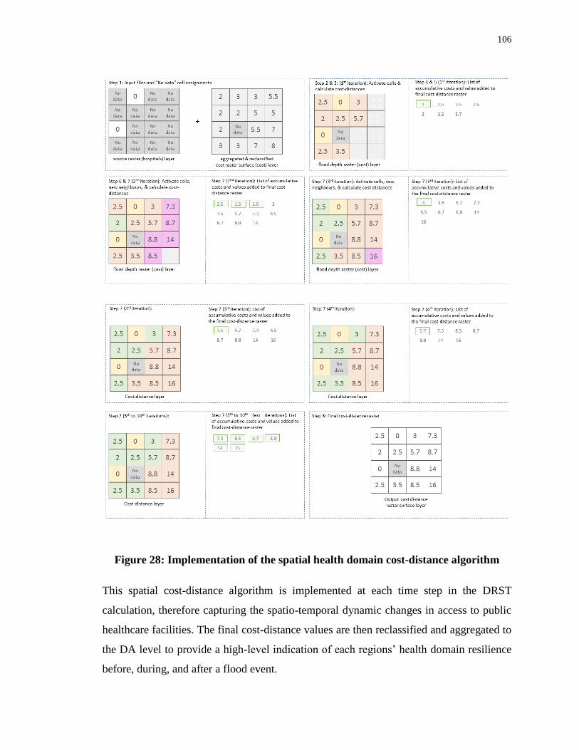
106
Figure 28: Implementation of the spatial health domain cost-distance algorithm
This spatial cost-distance algorithm is implemented at each time step in the DRST
calculation, therefore capturing the spatio-temporal dynamic changes in access to public
healthcare facilities. The final cost-distance values are then reclassified and aggregated to
the DA level to provide a high-level indication of each regions’ health domain resilience
before, during, and after a flood event.

107
The results of the health domain spatial analysis (Figure 29) is combined with regional
estimates of burden of disease and health impacts to provide a more complete estimate of
health domain resilience.
Figure 29: Health resilience spatial implementation, cost-distance workflow
diagram; this process is completed for each time step (t) in the simulation
Since this process involves the use of spatial data and spatial analysis techniques, health
resilience value will also be spatially (and temporally) dynamic. At each time step, health
domain resilience values are aggregated to the DA level, to achieve meaningful and
compatible spatial resilience results.
4.3.8 Social Domain: Description
Disasters have both tangible (relating to physical) and intangible (relating to emotional)
impacts on people. Therefore, it’s important to consider social resilience domain as part of

108
integrated disaster resilience assessment. Socially resilient populations demonstrate the
ability to adapt to a disturbance to better prepare for, respond to, and recover from disaster
circumstances. These populations may recover and emerge more resilient than they initially
were before the event occurred. Norris et al. (2008) suggested the following factors
influence social resilience: citizen involvement in mitigation efforts, ongoing psychosocial
support, strong civic leadership, and effective horizontal and vertical organizational
linkages. O’Neill et al. (2016) substantiate these claims through a review of available social
resilience literature, interviews with citizens, and through the author’s personal
experiences. They determined that the social resilience factors proposed by Norris et al.
(2008) were consistent with their findings in a case study following the 2009 flooding in
Fargo, North Dakota. They also propose that the community’s “identity” (in this case a
“floodplain identity”) heavily influences its social resilience in the event of a disturbance
(in this case a flood). These “identities” reflect a community’s attitudes, responsibilities,
and expectations of the government, relief organizations and individuals in the event of a
disturbance. It’s also been proposed that resilience of disaster management systems also
relies heavily on interorganizational and social networks, effective communication, trust,
and social capital (Kapucu and Demiroz, 2017). However, traditional disaster management
approaches, such as performance measurement tools, have faced challenges in evaluating
the relationships in – and between – these networks.
Disaster resilience at an individual level draws on knowledge gained from education,
previous experiences, personal interactions, and the media. The information from these
sources combines to formulate a perception which subsequently drives pre-disaster or post-
disaster actions (or inaction). In North America, people typically desire to live near the
coast; the close proximity to water makes it an attractive, popular, and hence expensive
location to live; coastal communities are often affiliated with affluent residents. In
developing countries however, people who have been displaced or rely on proximity to
water as a means of survival, live closest to the water, which makes them particularly
susceptible to impacts of hydrometeorological hazards. The disparity between these
scenarios can be captured by considering a spatio-temporal integrated disaster resilience.

109
The relationship between poverty, environmental degradation and hazard vulnerability is a
vicious, mutually reinforcing system of feedbacks (Kesavan and Swaminathan, 2006)
especially prevalent in developing countries. The degree to which persons may experience
physical, emotional, or psychological distress impacts is influenced by their tolerance and
coping capabilities in stressful situations.
4.3.9 Social Domain: Implementation
Based on literature and informal feedback collected during resilience building workshops,
connectivity was identified as one (of many) indicators of social disaster resilience. Social
resilience quantification was implemented in the DRST considering the performance
metric number of people with cellular service as a proxy for the connectivity resilience
indicator. Therefore, social system performance can be described as a function of the
following:
𝑃𝑐𝑜𝑛𝑛𝑒𝑐𝑡𝑖𝑣𝑖𝑡𝑦𝑠𝑜𝑐𝑖𝑎𝑙 =
𝑓(𝑛𝑜. 𝑜𝑓 𝑝𝑒𝑜𝑝𝑙𝑒 𝑠𝑒𝑟𝑣𝑖𝑐𝑒𝑑, 𝑜𝑝𝑒𝑟𝑎𝑡𝑖𝑜𝑛𝑎𝑙 𝑡𝑜𝑤𝑒𝑟𝑠, 𝑝𝑟𝑜𝑥𝑖𝑚𝑖𝑡𝑦 𝑡𝑜 𝑡𝑜𝑤𝑒𝑟, 𝑡𝑜𝑤𝑒𝑟 𝑐𝑎𝑝𝑎𝑐𝑖𝑡𝑦)
Since the provision of cellular service relies on the number of operational towers in the
area and subsequently depends on adequate power supply, the performance of this system
is also contingent on the power transmission network:
𝑜𝑝𝑒𝑟𝑎𝑡𝑖𝑜𝑛𝑎𝑙 𝑡𝑜𝑤𝑒𝑟𝑠 = 𝑓(𝑜𝑝𝑒𝑟𝑎𝑡𝑖𝑜𝑛𝑎𝑙 𝑠𝑢𝑏𝑠𝑡𝑎𝑡𝑖𝑜𝑛𝑠, 𝑡𝑟𝑎𝑛𝑠𝑚𝑖𝑠𝑠𝑖𝑜𝑛 𝑛𝑒𝑡𝑤𝑜𝑟𝑘)
When a disturbance occurs (such as a hazard event), it’s possible that the provision of
power is disrupted and connectivity is affected when a substation is no longer operational
and fails to deliver power to transmission lines, therefore rendering the cell towers not
operational. The implementation of the social sector is shown in Figure 30, an adapted
version of the methodology proposed by Andre et al. (2000)
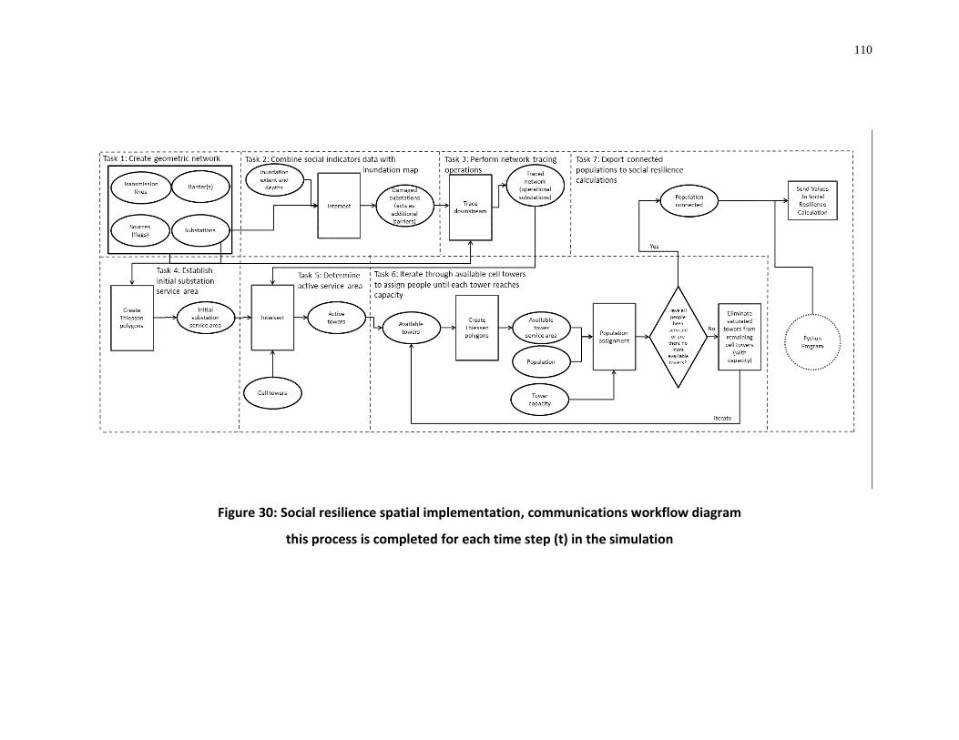
110
Figure 30: Social resilience spatial implementation, communications workflow diagram
this process is completed for each time step (t) in the simulation
111
Connectivity was the social resilience indicator selected to be implemented in this research,
however it’s possible as part of future work to include other social resilience indictors as
part of resilience quantification.
4.4 Integrated Resilience
The physical domain produces a times series of inundation maps which are used as input
into the DRST and directly influences economic, engineering, health, and social domains.
The engineering domain also provides input into the economic domain. These domains are
connected in spatial and temporal analysis via a middleware program created in the Python
programming language. This middleware program forms the crux of the analysis, linking
together GIS spatial datasets, spatial analysis, system dynamics simulation, and economic
optimization capabilities.
The proposed methodology currently integrates resilience measures from each domain
(economic, health, physical and social) into a single Resilience Index (RI) measure at each
time step (t) for each area (A), mathematically as:
𝑅𝐼 = ∑ 𝛼𝑖 𝑅𝑖 (4.19)
Where 𝛼𝑖 is a weighting factor, 𝑅𝑖 is each domain’s resilience value, and i is the domain
(physical, economic, health, and social). Expanded, this is:
𝑅𝐼 = 𝛼𝑖𝑅𝑖 + 𝛼2𝑅2 + 𝛼3𝑅3 + 𝛼4𝑅4 (4.20)
The weights, αi, were included to provide an opportunity to influence the resilience
calculation and could be adjusted to reflect decision maker priorities. Priorities could be
established through stakeholder workshops, discussions, or surveys. However, no
additional research into the selection of resilience weightings is provided as part of this
thesis.
112
4.5 DRST Programming and Simulation
The above relationships and model equations were implemented in a spatio-temporal
dynamic simulation tool called the Disaster Resilience Simulation Tool (DRST). The
resilience calculation is performed for each time step, for each domain, in the DRST. The
system dynamics simulation model is set up as a gaming simulation, which allows the user
to interact with the model to input model parameter values (from GIS) and make decisions
as the simulation progresses. The user can therefore participate in decisions that affect the
outcomes of the simulation. The next logical step would be to identify potential simulation
scenarios (various combinations of input variables) to see the potential impacts on disaster
resilience.
4.6 Adaptation Options
Implementing dynamic quantitative disaster resilience in a simulation tool provides an
opportunity to test various adaptation options. To inform the disaster management
community, it is necessary to conceptualize various opportunities and options for
increasing resilience through both structural and functional adaptation measures.
Adaptation options are best designed when they reflect local political and governance
structures whilst factoring in public perceptions and preferences. Therefore practical,
implementable options are best developed in consultation with local stakeholders.
Adaptation policies are incorporated into the model by considering adaptation scenarios as
part of the DRST. These scenarios are a combination of values assigned to a set of model
variables. The purpose of these scenarios is to observe changes in the city system resilience
as a result of implementing specific adaptation policies. The purpose of adaptation scenario
simulations is to help develop climate change adaptation policy, aid in resource allocation
decisions and prioritize disaster management investments.
The adaptation scenarios modify particular elements within the DRST to represent policy
actions. A scenario may modify initial values of input variables, or modification may be
implemented at another point during the simulation time horizon. For example, a scenario
may involve allocating additional financial resources to a particular model domain in the

113
period of response during a disaster. Another scenario may consider the effects of
allocating additional financial resources to a particular model domain in the period of
recovery after a disaster. These scenarios can be simulated separately in the DRST to
observe their effect on model subsystems and on overall resilience behaviour. Another
example of an adaptation scenario is designating additional emergency shelters before a
disaster in anticipation of coastal population growth and increased frequency of extreme
climate events. The expected system behaviour from this action would be an increase in
the STDRM and overall city resilience; the addition of emergency shelters would decrease
shelter crowding and likely reduce the spread of communicable disease in the event of a
disaster. However, this is an example of a direct, more obvious relationship associated with
the scenario; there may be other indirect relationships in the system that may be negatively
affected by this action. For example, increasing emergency shelters requires more
coordination and communication during disasters, increased funding for adequate
maintenance of buildings and possibly the employment of additional emergency support
personnel. The scenarios change input conditions which have cascading effects and can
modify subsystems of the resilience model. The results may be unforeseen consequences
in other domains that are less obvious than initially thought. The resilience system is
complex and the comprehensive DRST can help identify these direct and indirect
relationships and obvious and nonobvious system behaviour. It is desirable for adaptation
scenarios to be probable, realistic, and robust. Therefore, the three scenarios used to test
the DRST were selected in collaboration with experts familiar with the social-political
landscape in BC, Canada. Ultimately, the value in of this approach is not in providing a
single solution, but in providing an avenue for comparison between suites of different
scenario options, given the best information available.
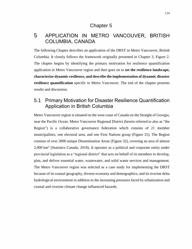
114
Chapter 5
5 APPLICATION IN METRO VANCOUVER, BRITISH COLUMBIA, CANADA
The following Chapter describes an application of the DRST in Metro Vancouver, British
Columbia. It closely follows the framework originally presented in Chapter 3, Figure 2.
The chapter begins by identifying the primary motivation for resilience quantification
application in Metro Vancouver region and then goes on to set the resilience landscape,
characterize dynamic resilience, and describe the implementation of dynamic disaster
resilience quantification specific to Metro Vancouver. The end of the chapter presents
results and discussion.
5.1 Primary Motivation for Disaster Resilience Quantification Application in British Columbia
Metro Vancouver region is situated on the west coast of Canada on the Straight of Georgia,
near the Pacific Ocean. Metro Vancouver Regional District (herein referred to also as “the
Region”) is a collaborative governance federation which consists of 21 member
municipalities, one electoral area, and one First Nations group (Figure 31). The Region
consists of over 3000 unique Dissemination Areas (Figure 32), covering an area of almost
2,900 km2 (Statistics Canada, 2018). It operates as a political and corporate entity under
provincial legislation as a “regional district” that acts on behalf of its members to develop,
plan, and deliver essential water, wastewater, and solid waste services and management.
The Metro Vancouver region was selected as a case study for implementing the DRST
because of its coastal geography, diverse economy and demographics, and its riverine delta
hydrological environment in addition to the increasing pressures faced by urbanization and
coastal and riverine climate change influenced hazards.
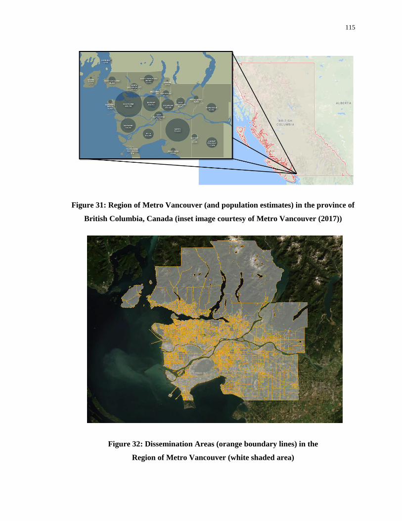
115
Figure 31: Region of Metro Vancouver (and population estimates) in the province of
British Columbia, Canada (inset image courtesy of Metro Vancouver (2017))
Figure 32: Dissemination Areas (orange boundary lines) in the
Region of Metro Vancouver (white shaded area)
116
The province of British Columbia has experienced an average temperature increase of
1.4°C in the last century (higher than the global average of 0.85°C), and temperatures
across the province are expected to continue to climb (BC Ministry of the Environment,
2016). The years 2015 and 2016 were two of the hottest years on record since 1900 due, at
least in part, to climate change combined with El Nino conditions and increased warm
nights due to increased cloud cover (Anslow, 2017). These changes in the climate are also
causing changes in the distribution, frequency, and intensity of precipitation events over
the region (Anslow, 2017). The region faces the combined threat of changes in peak flows
and flooding from the Fraser River and the threat posed by increasing sea levels from the
Pacific Ocean. Fortunately, the Region has recognized the threat of climate change and as
such, has developed a Corporate Climate Action Plan (Metro Vancouver, 2010). Two of
the most relevant Plan strategies to this work include “adapting existing infrastructure and
operations” and “planning and building resilient new infrastructure and facilities” in the
anticipation of climate change. Since then, the Region has also released a Strategic
Framework focused on ensuring infrastructure, ecosystems, and communities are resilient
to the impacts of climate change (Metro Vancouver, 2018). This framework explicitly
identifies the need to develop methods and approaches for measuring resilience to climate
change. Methodologies and tools such as the ones presented in this thesis, could help guide
the Region in prioritizing spending and developing effective climate change adaptation
policies in accordance with the strategies outlined in the Climate Action Plan and in support
of the guiding principles of the Climate 2050 Strategic Framework. It could also be useful
at the local scale for municipalities within the Region to help adapt to climate change
impacts.
Therefore, the primary motivation for applying the disaster resilience quantification
framework and methodology to the region of Metro Vancouver is two-fold:
i) To act as a proof-of-concept example for the work presented in this thesis; and
ii) To develop a tool that aligns with the Region’s climate initiatives and provides
a foundation for effective disaster management in Metro Vancouver.
117
5.2 Setting the Resilience Landscape: Research Questions and Problem Definition
In addition to acting as a proof-of-concept, the purpose of applying this research to the
Metro Vancouver region in British Columbia was to help answer climate change
adaptation-related questions that the local communities would be interested in resolving,
such as:
1. How are climate change influenced hydrometeorological hazards affecting Metro
Vancouver?;
2. How can municipalities in Metro Vancouver better plan for, and adapt to, future
climate change-influenced hydrometeorological hazards?; and
3. How resilient is Metro Vancouver to climate change influenced hazards?
In order to address these questions, the following research objectives were conceived for
the Metro Vancouver-specific application:
1. Identify climate change influenced hydrometeorological hazards which effect
communities in Metro Vancouver and incorporate climate change projections into
hazard modelling and inundation mapping;
2. Identify and simulate local disaster resilience adaptation options; and
3. Propose how outputs from the DRST could be used to improve climate change
mitigation and adaptation strategies at the local and regional levels.
The methodology from Figure 2 was implemented for the case study in order to simulate
disaster resilience, discover answers to the research questions, and achieve application
objectives:
1. Identify disaster resilience quantification system and metrics which are important
at the Regional scale;
2. Collect spatial and temporal data related to physical, economic, engineering, health,
and social disaster resilience domains;
3. Pre-process the data for use in the DRST using spatial and numerical tools;
118
4. Create a hydraulic model and simulate region-specific physical hazards including
climate change influenced SLR of the Pacific Ocean and climate change influenced
flooding on the Fraser River;
5. Identify potential local climate change adaptation strategies and use them to
develop corresponding climate change adaptation options for the DRST;
6. Modify DRST inputs and/or structures to represent adaptation options, as
necessary;
7. Simulate base case plus climate change and adaptation options using the DRST;
8. Post-process simulation results;
9. Compare adaptation option simulation results and identify times and areas of high
and low resilience.
The remainder of this chapter considers the case study specific application of resilience
quantification and the DRST at a Regional focal scale.
5.3 Implementation
The methodology behind resilience quantification was implemented in a primarily Python-
based DRST. This tool is able to extract spatial and attribute data from ArcGIS and use it
in combination with other numerical data as input into dynamic resilience calculations by
integrating it with Vensim and GAMS software. The following chapter describes a specific
application of the DRST and climate change influenced dynamic resilience assessment for
the region of Metro Vancouver in British Columbia, Canada.
5.3.1 Implementation: Data Collection and Identifying Key Elements to Describe Systems
Before fully implementing the STDRM and resilience quantification scheme, it was
necessary to establish what data were available to help describe the engineering, economic,
health, and social domain system models. Since resilience is dynamic in both time and
space, multiple data types were required to build the spatio-temporal model.
Spatial and numerical data were collected from various sources for use in the Metro
Vancouver DRST (Appendix E). Most of the data used in developing the Metro Vancouver
119
DRST were publicly available, with the exception of detailed economics and engineering
data which was provided by BC Assessment Corporation (BCA) and hydraulic modelling
validation data which were provided by the Ministry of Forest Lands and Natural Resource
Operations (MFLNRO).
Data for each resilience domain were collected in various formats including spatial and
numerical, and at various resolutions including city-wide, Dissemination Area (DA), and
feature-level (Figure 33). Therefore, significant effort was required to prepare data for
input into the DRST. Some of the necessary pre-processing was completed using query
statements and algorithms within a GIS environment; other data was modified manually.
The data collection process was intensive and the preprocessing of data (particularly spatial
data) required significant time investment. If data collection methods and formats were to
remain consistent in future versions of the tool, the DRST would benefit from automation
of these data preparation tasks. The preprocessed data files as used for input into the DRST
are included as part of the dissertation electronic submission. More details are provided in
Appendix F.
With a working knowledge of the available data and its limitations, the conceptual-level
generic DRST originally presented in Figure 14 was customized for an application specific
to quantifying disaster resilience in Metro Vancouver. A presentation of the system
dynamics simulation Vensim temporal model is provided in Figure 34. The model looks
a little sparse since many of the model relationships and dynamic feedbacks are spatial and
occur in the GIS (ArcPy) component of the DRST, however the use of system dynamics
simulation software, Vensim, provides an opportunity to expand the existing model and
incorporate additional disaster resilience indictors, domains, and systems. The current
version of the DRST system dynamic simulation model represents two key components of
the overall disaster resilience quantification scheme: (i) emergency disaster funding; and
(ii) disaster resilience calculation. Supporting model simulation equations are described in
this section.
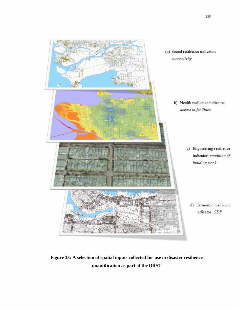
120
Figure 33: A selection of spatial inputs collected for use in disaster resilience
quantification as part of the DRST

121
Figure 34: Dynamic disaster resilience quantification Vensim model
The following equations describe the emergency funding component of the model, which
represents the amount of additional disaster assistance funding available during a disaster,
above and beyond local resources (Figure 35).
Figure 35: Emergency funding component of the DRST Vensim model
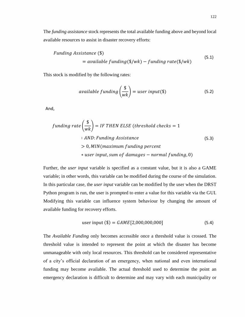
122
The funding assistance stock represents the total available funding above and beyond local
available resources to assist in disaster recovery efforts:
𝐹𝑢𝑛𝑑𝑖𝑛𝑔 𝐴𝑠𝑠𝑖𝑠𝑡𝑎𝑛𝑐𝑒 ($)
= 𝑎𝑣𝑎𝑖𝑙𝑎𝑏𝑙𝑒 𝑓𝑢𝑛𝑑𝑖𝑛𝑔($/𝑤𝑘) − 𝑓𝑢𝑛𝑑𝑖𝑛𝑔 𝑟𝑎𝑡𝑒($/𝑤𝑘) (5.1)
This stock is modified by the following rates:
𝑎𝑣𝑎𝑖𝑙𝑎𝑏𝑙𝑒 𝑓𝑢𝑛𝑑𝑖𝑛𝑔 ($
𝑤𝑘) = 𝑢𝑠𝑒𝑟 𝑖𝑛𝑝𝑢𝑡($) (5.2)
And,
𝑓𝑢𝑛𝑑𝑖𝑛𝑔 𝑟𝑎𝑡𝑒 ($
𝑤𝑘) = 𝐼𝐹 𝑇𝐻𝐸𝑁 𝐸𝐿𝑆𝐸 (𝑡ℎ𝑟𝑒𝑠ℎ𝑜𝑙𝑑 𝑐ℎ𝑒𝑐𝑘𝑠 = 1
∶ 𝐴𝑁𝐷: 𝐹𝑢𝑛𝑑𝑖𝑛𝑔 𝐴𝑠𝑠𝑖𝑠𝑡𝑎𝑛𝑐𝑒
> 0, 𝑀𝐼𝑁(𝑚𝑎𝑥𝑖𝑚𝑢𝑚 𝑓𝑢𝑛𝑑𝑖𝑛𝑔 𝑝𝑒𝑟𝑐𝑒𝑛𝑡
∗ 𝑢𝑠𝑒𝑟 𝑖𝑛𝑝𝑢𝑡, 𝑠𝑢𝑚 𝑜𝑓 𝑑𝑎𝑚𝑎𝑔𝑒𝑠 − 𝑛𝑜𝑟𝑚𝑎𝑙 𝑓𝑢𝑛𝑑𝑖𝑛𝑔, 0)
(5.3)
Further, the user input variable is specified as a constant value, but it is also a GAME
variable; in other words, this variable can be modified during the course of the simulation.
In this particular case, the user input variable can be modified by the user when the DRST
Python program is run, the user is prompted to enter a value for this variable via the GUI.
Modifying this variable can influence system behaviour by changing the amount of
available funding for recovery efforts.
user input ($) = 𝐺𝐴𝑀𝐸[2,000,000,000] (5.4)
The Available Funding only becomes accessible once a threshold value is crossed. The
threshold value is intended to represent the point at which the disaster has become
unmanageable with only local resources. This threshold can be considered representative
of a city’s official declaration of an emergency, when national and even international
funding may become available. The actual threshold used to determine the point an
emergency declaration is difficult to determine and may vary with each municipality or

123
even with each individual decision maker. The threshold value in this model can therefore
be modified by the user to best represent local decision maker profiles. The threshold value
is a threshold variable used to trigger access to the emergency funding assistance. This
variable is initialized as a constant, but can be modified by the user at the start of the
simulation via the DRST GUI:
𝑡ℎ𝑟𝑒𝑠ℎ𝑜𝑙𝑑 𝑣𝑎𝑙𝑢𝑒 = 𝐺𝐴𝑀𝐸[100,000,000] (5.5)
The sum of damages variable represents the current states of damages in the engineering
sector. It’s initialized as zero and assumes the value of building damages at each subsequent
time step.
𝑠𝑢𝑚 𝑜𝑓 𝑑𝑎𝑚𝑎𝑔𝑒𝑠 = 𝐺𝐴𝑀𝐸[0] (5.6)
The normal funding variable is used to represent resources available at the local level,
independent of additional (external) funding support. This variable is a constant in the
model and unlike many of the other variables in this sector of the model, is not a gaming
variable.
𝑛𝑜𝑟𝑚𝑎𝑙 𝑓𝑢𝑛𝑑𝑖𝑛𝑔 = 10,000,000 (5.7)
The above variables are then used as part of a threshold check to determine whether an
emergency has been declared which is subsequently used to release the emergency funds.
The threshold checks variable uses a conditional check with two criteria to be satisfied to
pass the check. One criterion is that the sum of damages in the engineering domain is
greater than the threshold value (representative of a declaration of emergency) and the
second criteria is that the sum of damages is greater than normal funding (actually exceeds
the local resource capacity). This prevents an emergency declaration to be declared without
necessity. If the checks are passed, a value of 1 (or TRUE) is sent to the funding rate
variable to release the additional funding assistance. If the checks are not passed, a value
of 0 (or FALSE) is passed to the funding rate variable.
𝑡ℎ𝑟𝑒𝑠ℎ𝑜𝑙𝑑 𝑐ℎ𝑒𝑐𝑘𝑠 = 𝐼𝐹 𝑇𝐻𝐸𝑁 𝐸𝐿𝑆𝐸(𝑠𝑢𝑚 𝑜𝑓 𝑑𝑎𝑚𝑎𝑔𝑒𝑠 > 𝑡ℎ𝑟𝑒𝑠ℎ𝑜𝑙𝑑 𝑣𝑎𝑙𝑢𝑒
∶ 𝐴𝑁𝐷: 𝑠𝑢𝑚 𝑜𝑓 𝑑𝑎𝑚𝑎𝑔𝑒𝑠 > 𝑛𝑜𝑟𝑚𝑎𝑙 𝑓𝑢𝑛𝑑𝑖𝑛𝑔, 1, 0) (5.8)

124
The reconstruction funding variable is representative of the amount of resources that is sent
to recovery efforts in the disaster resilience quantification sector of the Vensim model.
When emergency funds are released, they are added to the pool of regular funding:
𝑟𝑒𝑐𝑜𝑛𝑠𝑡𝑟𝑢𝑐𝑡𝑖𝑜𝑛 𝑓𝑢𝑛𝑑𝑖𝑛𝑔 = 𝑓𝑢𝑛𝑑𝑖𝑛𝑔 𝑟𝑎𝑡𝑒 + 𝑛𝑜𝑟𝑚𝑎𝑙 𝑓𝑢𝑛𝑑𝑖𝑛𝑔 (5.9)
The reconstruction funding is then distributed across the engineering and economic sectors
through the variable funding per building. This variable uses a conditional check to
distribute resources (equally) amongst the damaged buildings:
𝑓𝑢𝑛𝑑𝑖𝑛𝑔 𝑝𝑒𝑟 𝑏𝑢𝑖𝑙𝑑𝑖𝑛𝑔 = 𝐼𝐹 𝑇𝐻𝐸𝑁 𝐸𝐿𝑆𝐸(𝑛𝑢𝑚𝑏𝑒𝑟 𝑜𝑓 𝑏𝑢𝑖𝑙𝑑𝑖𝑛𝑔𝑠
= 0, 0, 𝑟𝑒𝑐𝑜𝑛𝑠𝑡𝑟𝑢𝑐𝑡𝑖𝑜𝑛 𝑓𝑢𝑛𝑑𝑖𝑛𝑔
/𝑛𝑢𝑚𝑏𝑒𝑟 𝑏𝑢𝑖𝑙𝑑𝑖𝑛𝑔𝑠 𝑑𝑎𝑚𝑎𝑔𝑒𝑑)
(5.10)
where,
𝑛𝑢𝑚𝑏𝑒𝑟 𝑏𝑢𝑖𝑙𝑑𝑖𝑛𝑔𝑠 𝑑𝑎𝑚𝑎𝑔𝑒𝑑 = 𝐺𝐴𝑀𝐸[0] (5.11)
The number buildings damaged is a GAME variable that is initialized to zero, but is
modified during the DRST simulation as this variable is retrieved from the DRST spatial
model. Subsequently, the funding per building variable then gets sent back to the GIS
spatial model at the end of the simulation time step.
Figure 36 illustrates the equations that describe the integrated disaster resilience
calculations component of the model.
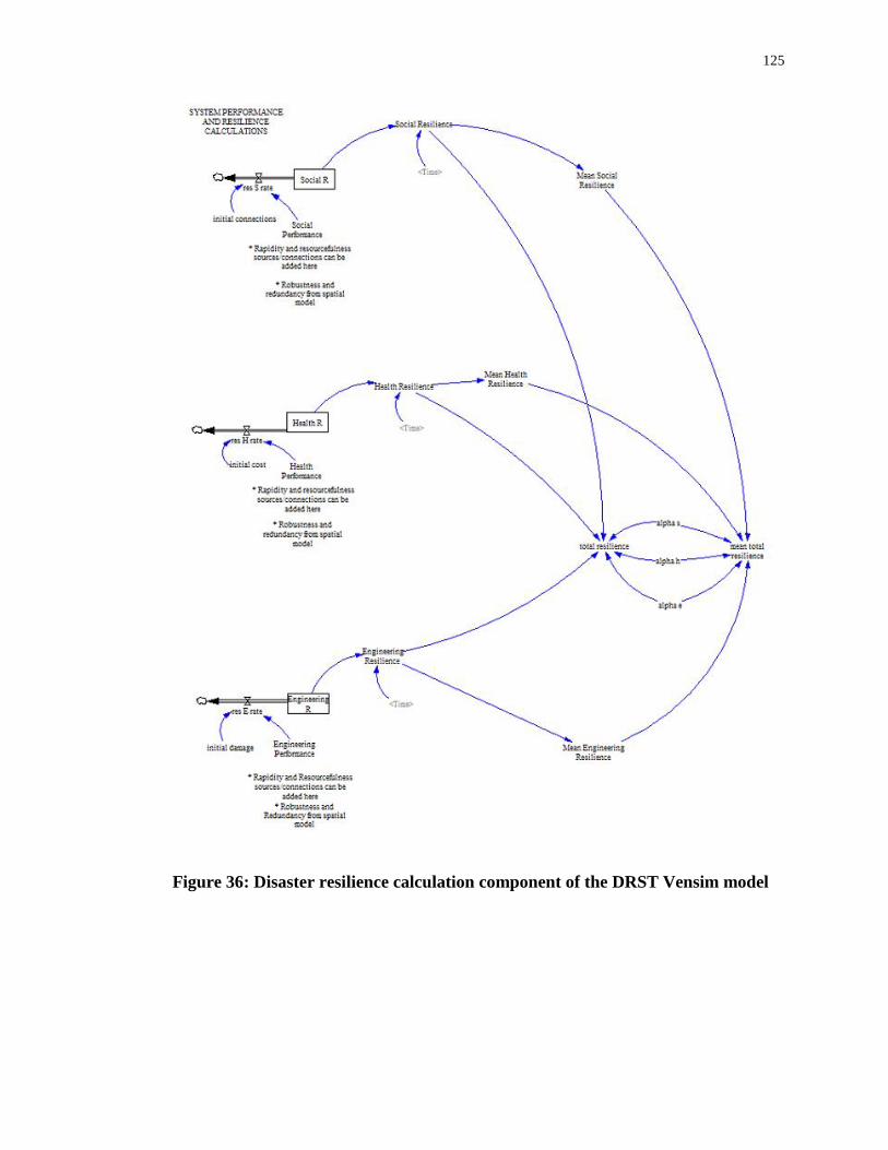
125
Figure 36: Disaster resilience calculation component of the DRST Vensim model
126
Resilience calculations for three of the four resilience domains are modelled in Vensim.
The primary relationships between model variables and model feedbacks are spatial and
are therefore represented in the ArcPy / GIS component of the DRST. The Vensim
modelling of resilience domains is used primarily to facilitate the resilience calculations.
Each of the domains (social, health, and engineering) has the same model structure, and
similar calculation for resilience quantification:
𝑆𝑜𝑐𝑖𝑎𝑙 𝑅[𝐷𝐴𝑈𝐼𝐷] = −𝑟𝑒𝑠𝑆𝑟𝑎𝑡𝑒[𝐷𝐴𝑈𝐼𝐷] (5.12)
𝐻𝑒𝑎𝑙𝑡ℎ 𝑅[𝐷𝐴𝑈𝐼𝐷] = −𝑟𝑒𝑠𝐻𝑟𝑎𝑡𝑒[𝐷𝐴𝑈𝐼𝐷] (5.13)
𝐸𝑛𝑔𝑖𝑛𝑒𝑒𝑟𝑖𝑛𝑔 𝑅[𝐷𝐴𝑈𝐼𝐷] = −𝑟𝑒𝑠𝐸𝑟𝑎𝑡𝑒[𝐷𝐴𝑈𝐼𝐷] (5.14)
The [𝐷𝐴𝑈𝐼𝐷] field stands for “Dissemination Area Unique ID”; it demarcates a subscript
in the model. The subscript allows the model to create as many structures as there are
subscript elements. This allows model variables to assume various values without having
to make multiple copies of the model structure. It simplifies the visual representation of
the system whilst also avoiding replication. In this particular application for Metro
Vancouver, the [𝐷𝐴𝑈𝐼𝐷] subscript is an array of over 3000 elements which represent
unique identifiers of each dissemination area in the model. This allows resilience
calculation for each domain to be performed at the DA level, across all the DAs in Metro
Vancouver. Although it may appear strange that there is no inflow into the stock, it is the
result of an implementation detail. Since the flow depends on variables sent from GIS, to
ease implementation just a single flow is represented, however the variable sent can assume
either a positive (+) or negative (-) value. The positive values deplete the resilience stock
and the negative values actually fill the stock since the expression of outflow is a negative
rate, creating a double negative which produces a positive flow. The equations for the
performance metric variables are as follows:
𝑆𝑜𝑐𝑖𝑎𝑙 𝑃𝑒𝑟𝑓𝑜𝑟𝑚𝑎𝑛𝑐𝑒[𝐷𝐴𝑈𝐼𝐷] = 𝐺𝐴𝑀𝐸[0] (5.15)
𝐻𝑒𝑎𝑙𝑡ℎ 𝑃𝑒𝑟𝑓𝑜𝑟𝑚𝑎𝑛𝑐𝑒[𝐷𝐴𝑈𝐼𝐷] = 𝐺𝐴𝑀𝐸[0] (5.16)
127
𝐸𝑛𝑔𝑖𝑛𝑒𝑒𝑟𝑖𝑛𝑔 𝑃𝑒𝑟𝑓𝑜𝑟𝑚𝑎𝑛𝑐𝑒[𝐷𝐴𝑈𝐼𝐷] = 𝐺𝐴𝑀𝐸[0] (5.17)
The performance variables are all initialized as zero, however this value is not important
to the calculation because these variables are designated as gaming variables which means
the value of the performance metric is retrieved from GIS at each time step. These variables
are also subscripted with [𝐷𝐴𝑈𝐼𝐷] which means the variable is calculated (retrieved) for
each dissemination area. The initialization of the Performance metric to a value of zero in
equation (5.17) is not significant to the simulation since there is a game variable in the
model which initializes each of the Performance metric using GIS data. Similarly, the
initialization variables are also GAME variables with initial values of zero:
𝐼𝑛𝑖𝑡𝑖𝑎𝑙 𝑐𝑜𝑛𝑛𝑒𝑐𝑡𝑖𝑜𝑛𝑠 [𝐷𝐴𝑈𝐼𝐷] = 𝐺𝐴𝑀𝐸[0] (5.18)
𝐼𝑛𝑖𝑡𝑖𝑎𝑙 𝑑𝑎𝑚𝑎𝑔𝑒 [𝐷𝐴𝑈𝐼𝐷] = 𝐺𝐴𝑀𝐸[0] (5.19)
𝐼𝑛𝑖𝑡𝑖𝑎𝑙 𝑐𝑜𝑠𝑡 [𝐷𝐴𝑈𝐼𝐷] = 𝐺𝐴𝑀𝐸[0] (5.20)
These initialization variables are set at the beginning of the simulation using performance
metric data drawn from GIS. These values are held for the remainder of the simulation to
normalize the performance metrics for the resilience calculation. A conditional statement
was used to define domain resilience, primarily for computational reasons in the system
dynamics simulation model:
𝑆𝑜𝑐𝑖𝑎𝑙 𝑅𝑒𝑠𝑖𝑙𝑖𝑒𝑛𝑐𝑒 = 𝐼𝐹 𝑇𝐻𝐸𝑁 𝐸𝐿𝑆𝐸 (𝑇𝑖𝑚𝑒
= 0, 𝑆𝑜𝑐𝑖𝑎𝑙𝑅[𝐷𝐴𝑈𝐼𝐷], 𝑆𝑜𝑐𝑖𝑎𝑙𝑅[𝐷𝐴𝑈𝐼𝐷]/𝑇𝑖𝑚𝑒) (5.21)
𝐻𝑒𝑎𝑙𝑡ℎ 𝑅𝑒𝑠𝑖𝑙𝑖𝑒𝑛𝑐𝑒 = 𝐼𝐹 𝑇𝐻𝐸𝑁 𝐸𝐿𝑆𝐸 (𝑇𝑖𝑚𝑒
= 0, 𝐻𝑒𝑎𝑙𝑡ℎ𝑅[𝐷𝐴𝑈𝐼𝐷], 𝐻𝑒𝑎𝑙𝑡ℎ𝑅[𝐷𝐴𝑈𝐼𝐷]/𝑇𝑖𝑚𝑒)
(5.22)
𝐸𝑛𝑔𝑖𝑛𝑒𝑒𝑟𝑖𝑛𝑔 𝑅𝑒𝑠𝑖𝑙𝑖𝑒𝑛𝑐𝑒 = 𝐼𝐹 𝑇𝐻𝐸𝑁 𝐸𝐿𝑆𝐸 (𝑇𝑖𝑚𝑒
= 0, 𝐸𝑛𝑔𝑖𝑛𝑒𝑒𝑟𝑖𝑛𝑔𝑅[𝐷𝐴𝑈𝐼𝐷], 𝐸𝑛𝑔𝑖𝑛𝑒𝑒𝑟𝑖𝑛𝑔𝑅[𝐷𝐴𝑈𝐼𝐷]/𝑇𝑖𝑚𝑒)
(5.23)
128
This condition prevents an indeterminate error from being thrown at 𝑡𝑖𝑚𝑒 = 0. These
resilience values are then spatially aggregated across DAs to reflect a city-wide resilience
metric over time:
𝑀𝑒𝑎𝑛 𝑆𝑜𝑐𝑖𝑎𝑙 𝑅𝑒𝑠𝑖𝑙𝑖𝑒𝑛𝑐𝑒
= 𝑆𝑈𝑀(𝑆𝑜𝑐𝑖𝑎𝑙 𝑅𝑒𝑠𝑖𝑙𝑖𝑒𝑛𝑐𝑒[𝐷𝐴𝑈𝐼𝐷!])/𝐸𝐿𝑀𝐶𝑂𝑈𝑁𝑇(𝐷𝐴𝑈𝐼𝐷)
(5.24)
𝑀𝑒𝑎𝑛 𝐻𝑒𝑎𝑙𝑡ℎ 𝑅𝑒𝑠𝑖𝑙𝑖𝑒𝑛𝑐𝑒
= 𝑆𝑈𝑀(𝐻𝑒𝑎𝑙𝑡ℎ 𝑅𝑒𝑠𝑖𝑙𝑖𝑒𝑛𝑐𝑒[𝐷𝐴𝑈𝐼𝐷!])/𝐸𝐿𝑀𝐶𝑂𝑈𝑁𝑇(𝐷𝐴𝑈𝐼𝐷)
(5.25)
𝑀𝑒𝑎𝑛 𝐸𝑛𝑔𝑖𝑛𝑒𝑒𝑟𝑖𝑛𝑔 𝑅𝑒𝑠𝑖𝑙𝑖𝑒𝑛𝑐𝑒
= 𝑆𝑈𝑀(𝐸𝑛𝑔𝑖𝑛𝑒𝑒𝑟𝑖𝑛𝑔 𝑅𝑒𝑠𝑖𝑙𝑖𝑒𝑛𝑐𝑒[𝐷𝐴𝑈𝐼𝐷!])
/𝐸𝐿𝑀𝐶𝑂𝑈𝑁𝑇(𝐷𝐴𝑈𝐼𝐷)
(5.26)
These average values are then combined in the 𝑇𝑜𝑡𝑎𝑙 𝑅𝑒𝑠𝑖𝑙𝑖𝑒𝑛𝑐𝑒[𝐷𝐴𝑈𝐼𝐷] variable using
weights, α as follows:
𝑇𝑜𝑡𝑎𝑙 𝑅𝑒𝑠𝑖𝑙𝑖𝑒𝑛𝑐𝑒[𝐷𝐴𝑈𝐼𝐷]
= 𝑎𝑙𝑝ℎ𝑎𝑆 ∗ 𝑚𝑒𝑎𝑛 𝑠𝑜𝑐𝑖𝑎𝑙 𝑟𝑒𝑠𝑖𝑙𝑖𝑒𝑛𝑐𝑒[𝐷𝐴𝑈𝐼𝐷] + 𝑎𝑙𝑝ℎ𝑎𝐸
∗ 𝑚𝑒𝑎𝑛 𝑒𝑛𝑔𝑖𝑛𝑒𝑒𝑟𝑖𝑛𝑔 𝑟𝑒𝑠𝑖𝑙𝑖𝑛𝑒𝑐𝑒[𝐷𝐴𝑈𝐼𝐷] + 𝑎𝑙𝑝ℎ𝑎𝐻
∗ 𝑚𝑒𝑎𝑛 ℎ𝑒𝑎𝑙𝑡ℎ 𝑟𝑒𝑠𝑖𝑙𝑖𝑒𝑛𝑐𝑒[𝐷𝐴𝑈𝐼𝐷]
(5.27)
The alpha, α, weights [0,1] are intended to capture decision maker priorities. This provides
an opportunity for decision makers to directly influence the resilience calculation. Weights
for this particular application were not established with stakeholders and were therefore set
to a value of 1 in the model, however determining appropriate weights could be an area of
future work. The system dynamics model was then run considering continuous flood
hazard simulations to test the impact that various adaptation options have on resilience.
5.3.2 Implementation: Climate Change Influenced Hazard Definition
As a coastal and mountainous province, British Columbia (BC) has unique climate and
topography and is no stranger to riverine and coastal flooding. As such, a history of
hydraulic modelling and floodplain mapping has developed in BC. There is an extensive

129
levee network along the Fraser River and its tributaries which contributes to the hydraulic
characteristics of the basin. The remainder of this sub-section will describe the modelling
and simulation procedure used to generate a set of dynamic inundation maps for the Fraser
River under climate change. This sub-section concludes with the results for generating
inundation maps considering climate change. These maps are used for hazard
characterization and serves as one of the primary inputs into the DRST.
5.3.2.1 British Columbia climate and topography
BC has high spatial climate variability due to its unique topography and proximity to both
coastal and inland waters. BC is also characterized by wide variations in land elevation
including the highly mountainous Rockies region inland and very low coastal delta regions
near the ocean (Figure 37). The topography of the landscape is shaped, in part, by
hydrological processes. In turn, the topography is fundamental to defining regional flow
characteristics. This concept is fundamental to understanding hydrologic and hydraulic
dynamics within a catchment.
(a)
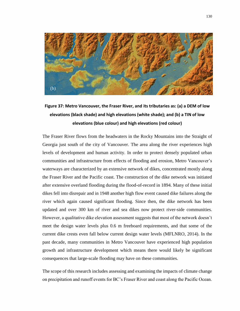
130
Figure 37: Metro Vancouver, the Fraser River, and its tributaries as: (a) a DEM of low
elevations (black shade) and high elevations (white shade); and (b) a TIN of low
elevations (blue colour) and high elevations (red colour)
The Fraser River flows from the headwaters in the Rocky Mountains into the Straight of
Georgia just south of the city of Vancouver. The area along the river experiences high
levels of development and human activity. In order to protect densely populated urban
communities and infrastructure from effects of flooding and erosion, Metro Vancouver’s
waterways are characterized by an extensive network of dikes, concentrated mostly along
the Fraser River and the Pacific coast. The construction of the dike network was initiated
after extensive overland flooding during the flood-of-record in 1894. Many of these initial
dikes fell into disrepair and in 1948 another high flow event caused dike failures along the
river which again caused significant flooding. Since then, the dike network has been
updated and over 300 km of river and sea dikes now protect river-side communities.
However, a qualitative dike elevation assessment suggests that most of the network doesn’t
meet the design water levels plus 0.6 m freeboard requirements, and that some of the
current dike crests even fall below current design water levels (MFLNRO, 2014). In the
past decade, many communities in Metro Vancouver have experienced high population
growth and infrastructure development which means there would likely be significant
consequences that large-scale flooding may have on these communities.
The scope of this research includes assessing and examining the impacts of climate change
on precipitation and runoff events for BC’s Fraser River and coast along the Pacific Ocean.
(b)
131
The purpose in performing this analysis is to generate climate change influenced
inundation maps which form the basis for resilience assessment using the DRST.
5.3.2.2 Brief history of hydraulic modelling and floodplain mapping in British Columbia
Inundation maps are primarily used to identify areas susceptible to flooding; typically near
water-bodies such as oceans, rivers, lakes and marshes. The identification of these areas is
especially important for infrastructure design, maintenance and protection. In addition,
inundation maps are frequently used to form the technical basis for land use planning,
community development bylaws, emergency planning, and flood hazard management
(Kerr Wood Leidal Associates Ltd., 2011). These maps are the basis for DRST hazard
assessment. They incorporate the effects of climate change in the basin and are the direct
input into the DRST.
A floodplain mapping agreement officially known as, “An Agreement Respecting
Floodplain Mapping in the Province of British Columbia” was signed in 1987 and amended
in 1994 between Canada and the province of British Columbia which addressed, among
other items:
Restricted development by both governments in flood vulnerable areas;
Required flood protection measures be incorporated into new development areas in
floodplains;
Recognized the need for updated flood mapping programs and integrated water
resources management.
In 2004, the Province of BC transferred the all aspects of floodplain mapping and related
decision-making responsibilities to local governments (Kerr Wood Leidal Associates Ltd.,
2011). The province no longer financially supported the development or maintenance of
floodplain maps.
In 2011, Kerr Wood Leidal released a report for the MFLNRO on Coastal Floodplain
Mapping Guidelines and Specifications which provides suggestions for design flood

132
construction levels (FCLs), introduces new standards for provincial topographic mapping,
and encourages local governments to develop coastal floodplain maps based on best
practices (Kerr Wood Leidal Associates Ltd., 2011). In partial fulfillment of the
recommendations, the Fraser Basin Council (FBC) updated the design flood profile for the
Fraser River and in 2005 Northwest Hydraulic Consultants (NHC) was retained to develop
a 1-D MIKE 11 hydraulic model for the Fraser River from Sumas Mountains to Georgia
Strait (NHC, 2008). This model was then taken over by the BC Ministry of Forests, Lands
and Natural Resource Operations (MFLNRO) and updated in 2014 using new data from
2007, 2011, and 2012 for re-calibration. The most recent publicly available report (June
2014 at the time of this thesis) contained output from hydraulic analyses in the form of
water levels at various locations along the river under two climate scenarios. There is
extensive hydraulic analysis and discussion in the 2014 report. However, the model was
run under an assumption which makes it inappropriate for the DRST, specifically:
“At the locations where “levees” are specified in the model x-sections, the model assumes
glass walls in case the water level goes higher than the levee top (or dike crest) and does
not allow any spillage. In the case a dike is breached or overtopped, the actual water levels
would be different from the model water levels.”
Flood Safety Section, Ministry of Forests, Lands, and Natural Resource
Operations 2014, pg. 23
This assumption restricts the model and prevents simulation of any over bank flooding.
Not only is this assumption rather optimistic and improbable, it could also be construed as
misleading by indirectly suggesting that communities along the Fraser River do not need
to anticipate or prepare for flood events. Thus, the results from this report could not be used
and therefore it was necessary to devise a means to generate inundation maps considering
both riverine flooding and SLR under climate change to be used as input into the DRST.
As such, the hydraulic model had to satisfy the following criteria:
Simplified model development;
Rapid simulation;

133
Use of widely accepted methods in the hydrologic and engineering communities;
Be calibrated to observed historical events;
Be able to incorporate climate change;
To the best of its ability, be able to simulate realistic water surface profiles;
Allow easy incorporation of new floodplain data, should it become available in the
future.
Based on the criteria above, hydraulic modelling was performed using the US Army Corps
of Engineers HEC-RAS hydraulic modelling software combined with the HEC-GeoRAS
extension. HEC-RAS was used for hydraulic modelling calculations and HEC-GeoRAS is
an extension compatible with ArcMap software, used to prepare geospatial inputs and
process geospatial outputs of the HEC-RAS simulation. This follows the same generic
procedure as outlined in the description of the physical hazard model domain.
5.3.2.3 Climate change scenarios
Climate change scenarios were required to obtain spatial and temporal estimates for future
regional climate variables, including precipitation. The climate change scenarios used in
developing inundation maps in this study were provided by Pacific Climate Impacts
Consortium (PCIC) in 2014; the bias-corrected models and streamflow projection datasets
have since been made publicly available online through PCIC’s website. PCIC used a set
of scenarios to generate estimates of precipitation which were subsequently used in
hydrologic modelling to generate estimates of future streamflow. PCIC employed the use
of three climate change emissions scenarios (A1B, A2, and B1) and eight GCMs initially
proposed in the IPCC’s AR4. GCM outputs were then downscaled using the Bias Corrected
Spatial Disaggregation (BCSD) method (Werner, 2011). Additional information on the
basis of climate change scenarios selection can be found in (Shrestha et al., 2012). These
climate change scenarios were used to generate climate change influenced inundation
mapping for Metro Vancouver.
134
5.3.2.4 Climate change influenced hazard modelling: Hydrology
Shrestha et al. (2012) discovered that, generally, peak streamflows in the Fraser River basin
are likely to decrease in the future. However, an increase in overall streamflow volumes is
likely to be observed. As input into the DRST, peak streamflows are of primary interest in
order to simulate large-scale, widespread flood events, and are therefore used to describe
the hydrological events of interest. Hydrologic modelling was then implemented to obtain
streamflows for the Fraser River and its tributaries under the conditions of various climate
scenarios.
The spatially distributed hydrologic modelling and simulation for the region was conducted
by Pacific Climate Impacts Consortium (PCIC) at the University of Victoria using the
Variable Infiltration Capacity (VIC) hydrologic model (Shrestha et al., 2012). Using
observed regional historical precipitation data, GCMs, and IPCC’s SRES A1B, A2, and B1
emissions scenarios, PCIC generated streamflows using the VIC hydrologic model. The
hydrologic simulation was conducted and streamflows generated for four locations
corresponding to the following Water Survey of Canada gauge locations (Figure 38):
1. Fraser River at Mission (08MH024) – FRSMI
2. Fraser River at Hope (08MF005) – FRSHP
3. Chilliwack River at Vedder Crossing (08MH001) – CHILL
4. Harrison River near Harrison Hot Springs (08MG013) – HARRI
PCIC generated streamflows for 24 scenarios: 1 base case and 23 simulations based on
climate projections (Table 4); the GCMs (based on the World Climate Research Program’s
Coupled Model Inter-Comparison Phase 3 Project) and SRES emissions scenarios A1B,
A2, and B1 from IPCC AR4. PCIC provided the streamflow data at both daily and monthly
time scales, with flows for multiple GCMs under all three emissions scenarios, for each of
the four WSC gauge sites (Figure 38). The projected streamflows are from 2050 – 2098
(48 years) and the base run covers 1950 – 2006 (56 years). As input into hydraulic

135
modelling for Metro Vancouver, a subset of the projected streamflows (CGCM3-AlB and
CGCM3-B2) plus the base case were selected.
Figure 38: The four Water Survey of Canada gauge sites (08MH024; 08MF005;
08MH001; 08MG013) in British Columbia along the Fraser River and its tributaries
(provided by Markus Shnorbus, PCIC 2014)
Table 4: Streamflow projection availability through PCIC Portal for selected GCM
and emissions scenarios
Scenario
GCM A1B A2 B1
HadCM Y Y Y
GFDL2.1 Y Y Y

136
CSIRO35 Y Y Y
CCSM3 Y Y Y
HadGEM1 Y Y N
MIROC3.2 Y Y Y
CGCM3 Y Y Y
ECHAM5 Y Y Y
Historical - - -
Annual streamflow maxima were fit to various continuous probability distribution
functions using an R statistical modelling package to determine which distribution
provided the best fit. Based on shape, scale, and location parameter estimations using L
moment of methods, it was determined that most of the streamflow extremes were best
described using a 3-parameter Weibull distribution:
𝑓(𝑥; 𝑘, 𝜆, 𝜃) =𝑘
𝜆(
𝑥 − 𝜃
𝜆)
𝑘−1
𝑒−(
𝑥−𝜃𝜆
)𝑘
(5.28)
where, k is the shape parameter, λ is the scale parameter, and θ is the location parameter.
Significant differences can be observed in the annual peak maximums between the baseline
and climate change scenarios for each of the 100-, 200-, and 500-year peak streamflows
(Table 5). However, only minor differences are observed between each of the two selected
climate change scenarios (A1B and B1). Lowest flows were observed in the baseline
scenario and the highest flows were observed in the simulated A1B emissions scenario.
The 500-year baseline, B1, and A1B streamflow scenarios were selected to generate water
surface profiles for the subsequent hydraulic analysis to capture extreme flooding
conditions.

137
Table 5: Statistical 100-, 200-, and 500-year streamflow values for three climate
scenarios and four stream gauge locations along the Fraser River and its tributaries
Branch/Tributary
Climate
Scenario
Chilliwack at
Vedder
(08MH001)
Fraser at
Hope
(08MF005)
Harrison
River
(08MG013)
Fraser at
Mission
(08MH024)
Baseline
Parameters
Location 247 7850 1335 9346
Scale 78 1488 203 1699
Shape 0.16 -0.41 -0.18 -0.38
Streamflows
(m3/s)
100-yr 779 10934 1973 13028
200-yr 900 11071 2031 13207
500-yr 1081 11202 2098 13382
Climate
Scenario
A1B
Parameters
Location 354 8063 1358 9512
Scale 179 1651 260 1912
Shape 0.2 -0.13 -0.12 -0.15
Streamflows
(m3/s)
100-yr 1692 13768 2281 15859
200-yr 2022 14369 2382 16490
500-yr 2533 15083 2503 17228
Climate
Scenario
B1
Parameters
Location 322 7901 1289 9334
Scale 115 1447 199 1616
Shape 0.24 -0.15 -0.09 -0.16
Streamflows 100-yr 1300 12719 2041 14544

138
(m3/s) 200-yr 1568 13200 2131 15041
500-yr 1999 13764 2240 15615
Inflow hydrographs were generated for the 500-year streamflow on the Fraser River at
Hope (WSC gauge 08MF005) and the two tributaries Chilliwack at Vedder (gauge
08MH001) and Harrison River (gauge 08MG013). This is equivalent to simulating the 1
in 500-year events for each tributary, which does not necessarily produce a 500-year event
at downstream gauges, but it does provide a “worst case scenario” to simulate the situation
in which all reaches simultaneously experience a 1 in 500-year event.
The files used in the current analysis were provided directly by PCIC, however since
January 2014 and September 2014, PCIC have made streamflows and gridded hydrologic
model outputs and statistically downscaled climate scenarios projections publicly available
through their data portal page (Pacific Climate Impact Consortium, 2014).
5.3.2.5 Climate change influenced hazard modelling: Hydraulics
Hydraulic modelling was then completed to generate water surface profile (i.e. water
levels) and inundation maps for the Fraser River under various climate change scenarios.
The water surface elevations were converted into inundation maps using spatial analyst
tools in ArcGIS.
HEC-RAS software was used for hydraulic analysis. This software was developed and used
by the United States by the US Army Corps of Engineers for hydraulic analysis. The
MFLNRO uses the proprietary 1-D modelling software called MIKE11 (DHI) for their
hydraulic analyses and flood forecasting model. The following procedure is somewhat
unique to the preparation, modelling, and simulation using HEC-RAS software, but the
procedure shared many similarities to the way MIKE11 data, modelling, and simulation
would be prepared and performed. The procedure would be similar to derive the input for
the MIKE11 model as described in NHC (2008). An overview of the processes is provided
in the following section.
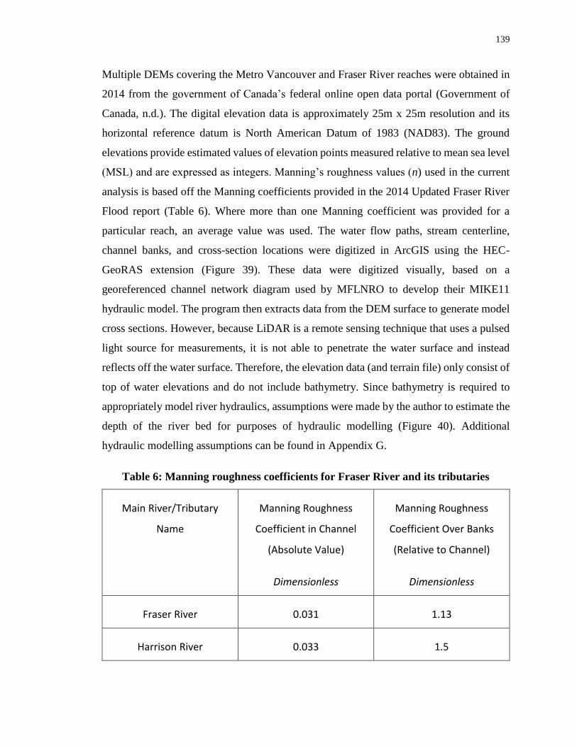
139
Multiple DEMs covering the Metro Vancouver and Fraser River reaches were obtained in
2014 from the government of Canada’s federal online open data portal (Government of
Canada, n.d.). The digital elevation data is approximately 25m x 25m resolution and its
horizontal reference datum is North American Datum of 1983 (NAD83). The ground
elevations provide estimated values of elevation points measured relative to mean sea level
(MSL) and are expressed as integers. Manning’s roughness values (n) used in the current
analysis is based off the Manning coefficients provided in the 2014 Updated Fraser River
Flood report (Table 6). Where more than one Manning coefficient was provided for a
particular reach, an average value was used. The water flow paths, stream centerline,
channel banks, and cross-section locations were digitized in ArcGIS using the HEC-
GeoRAS extension (Figure 39). These data were digitized visually, based on a
georeferenced channel network diagram used by MFLNRO to develop their MIKE11
hydraulic model. The program then extracts data from the DEM surface to generate model
cross sections. However, because LiDAR is a remote sensing technique that uses a pulsed
light source for measurements, it is not able to penetrate the water surface and instead
reflects off the water surface. Therefore, the elevation data (and terrain file) only consist of
top of water elevations and do not include bathymetry. Since bathymetry is required to
appropriately model river hydraulics, assumptions were made by the author to estimate the
depth of the river bed for purposes of hydraulic modelling (Figure 40). Additional
hydraulic modelling assumptions can be found in Appendix G.
Table 6: Manning roughness coefficients for Fraser River and its tributaries
Main River/Tributary
Name
Manning Roughness
Coefficient in Channel
(Absolute Value)
Dimensionless
Manning Roughness
Coefficient Over Banks
(Relative to Channel)
Dimensionless
Fraser River 0.031 1.13
Harrison River 0.033 1.5
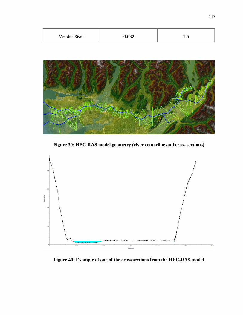
140
Vedder River 0.032 1.5
Figure 39: HEC-RAS model geometry (river centerline and cross sections)
Figure 40: Example of one of the cross sections from the HEC-RAS model

141
5.3.2.6 Climate change influenced hazard modeling as model boundary conditions
In order to assess the impacts of climate change on coastal cities more completely,
projections of sea level rise (SLR) were required. The DRST uses these SLR projections
to determine effects on coastal and riverine water levels and possible long-term climate
change impacts to coastal regions. The IPCC AR4 and AR5 identify SLR as a significant
hazard to coastal cities. AR5 introduced four new emissions scenarios called
Representative Concentration Pathways (RCPs). These RCPs are all based on different
degrees of radiative forcing, under scenario-specific assumptions, and were developed by
different organizations. Therefore, there is no direct correlation between them. They are
used to capture the effects of changes in GHG concentrations on climate variables; they
are the climate change component of SLR analysis.
The SLR modelling and projections were completed by Agam (2014). The projections of
sea level rise and global mean temperature presented in AR5 are not temporally or spatially
uniform and therefore a regional-scale model was developed by Agam (2014). The global
SLR projections were then analyzed in the context of two significant regional
hydrodynamic considerations for the Metro Vancouver Area: ocean tides and vertical land
movements. Sea level rise projections for the region of Metro Vancouver, including
influences of the local tides near the Fraser River, are in Agam (2014).
These SLR projections - in addition to the aforementioned climate change influenced
hydrologic model outputs - were then used in hydraulic modelling and simulation. The
mean water surface elevations serve as boundary conditions in the hydraulic model at the
four outlets of the Fraser River into the Pacific Ocean. In an effort to minimize the amount
of data, simulation and post-processing required, only two of the RCP scenarios (RCP2.6
and RCP8.5) were selected in the process of generating inundation maps. RCP2.6 and
RCP8.5 provide the lower and upper boundaries, respectively, of the RCP scenarios. This
reduces the uncertainty associated with selecting a single climate model or RCP scenario
and was able to capture a broad range of possible climate change impacts. Therefore, three
hydraulic model boundary conditions were considered in this study: RCP2.6 (2100);
RCP8.5 (2100) and base case (no SLR).

142
5.3.2.7 Hydraulic Modelling Results
There is no basis for assuming that trends in historic data will continue into the future.
Therefore, the modified streamflow datasets were used in hydraulic modelling. The use of
continuous hydraulic simulation was applied to investigate the inundation extent and
depths of sea level rise and climate change influenced riverine flooding. The methodology
applied in continuous hydraulic simulation was ultimately the application of a novel dataset
in conjunction with traditional modelling techniques. Continuous simulation provided an
improved understanding of the riverine response to sea level rise, which may ultimately
inform the future evaluation of coastal and interior climate change adaptation decisions.
The inundation maps generated for other scenarios are included in Appendix F.
Additional work is recommended to establish a definitive linkage between observed trends
and climate change for the Fraser River Basin. The approach adopted in this application is
subject to unquantifiable uncertainty but recognizes the non-stationarity of historic peak
flows for the purposes of hydraulic modelling and simulation and ultimately, for hazard
definition as part of demonstrating the disaster resilience quantification framework for use
in the DRST.
5.3.3 Implementation: Generating Adaptation Options
A simulation scenario represents specific courses of action that modifies system input.
These scenarios are designed to test system response to a set of input conditions
(Simonovic S. P., 2009) and may be used to represent a policy. The purpose of simulating
various adaptation scenarios is to observe changes in resilience as model output; this way
the resilience may be used as the decision making criteria in selecting adaptation scenarios
which offer the highest increase in system resilience. The same model can be tested under
various simulation scenarios to compare behavior under different sets of input conditions.
Real policy systems are highly nonlinear in behaviour and often conflict or reinforce each
other. Therefore, in some cases, the impact of policy decisions in a combination of
particular resilience components may be of more interest than the sum of their impacts.
The manner in which a municipality formulates policy decisions is not explicitly
represented in the DRST but is incorporated as a set of adaptation scenarios. For example,
143
the decision to increase number of emergency responders and safety personnel, or to
coordinate allocation of resources for before, during, and after a disaster event. To examine
the potential effectiveness of these types of options, three hypothetical adaptation scenarios
were simulated using the DRST. The process for developing and implementing adaptation
scenarios is discussed further in this section.
The three adaptation scenario options being tested with the DRST represent potential non-
structural measures in the categories of: mobile health services, managed retreat, and
funding.
1. The first adaptation option is non-structural; to provide access to additional
emergency health services during a disaster via a mobile hospital. For many
individuals, access to a hospital during a disaster event can become quite
challenging and so this option simulates a mobile station that becomes active
part-way through the simulation (at time step 6).
2. The second adaptation option is non-structural; managed retreat from the Pitt
Meadows community in Burnaby, BC. This option assumes that the properties
in the Pitt Meadows community are purchased by the government and the
population is relocated elsewhere, outside of the floodplain. The land therefore
no longer supports commercial or residential activities.
3. The third adaptation option is non-structural; access to additional sources of
funding. This option uses a threshold value which is intended to represent the
time at which an emergency declaration is made. Declaring an emergency
provides access to additional funding sources which may include federal or
international aid. This option specifies aid in terms of dollars, however those
dollars could actually reflect various types of resource supplies. The money
could be used to purchase mobile health units, mobile cellular towers, or used
to hire additional contractors to help rebuild damaged homes. The additional
funding is only accessed once the threshold is crossed, otherwise systems
function under “normal” conditions rather than “emergency” conditions.

144
Systems do not have access to any additional funding until emergency
conditions are satisfied.
This list of scenarios is not exhaustive, and there are an unlimited number of potential
adaptation options that could be tested using the DRST; these three just provide an
illustrative selection of possible non-structural options. These three options were identified
as a few of the more robust, plausible, and possible options likely to be considered in the
socio-political context of Metro Vancouver and were selected in consultation with local
stakeholders. These options could be expanded to include potential structural adaptation
options.
Various combinations of hydraulic modelling scenarios, SLR scenarios, and adaptation
options were tested using the DRST (Table 7). Together, these combinations represent a
very small selection of alternatives that could be tested using the DRST. Any combination
of riverine climate scenario, sea level rise scenario, and hydraulic event could be simulated
in the DRST. However, a subset of these scenario combinations was selected for illustrative
purposes. Two SRES-based hydraulic climate scenarios plus baseline were modeled to
represent a lower and upper range of potential riverine impacts. Since the A1B scenario
generates more significant flooding extent and depths than the baseline scenario, it would
likely result in greater impacts and was therefore carried forward to be modeled in
combination with the various adaptation options. Only the 500-Year riverine flooding
event was simulated since the Fraser River diking network is designed to provide levels of
protection above the (current) 200-Year event. Even modeling a 200-Year climate change
influenced riverine flooding event does not yield significant flooding in Metro Vancouver
and it was therefore deemed an inadequate proof-of-concept example. The 500-Year
climate change influenced riverine flood event results in fairly significant flood extent and
depths across Metro Vancouver and thus, the 500-Year event was carried forward and used
in all of the proof-of-concept simulation scenarios. The lower bound sea level rise scenario
(RCP 2.6) was selected for most of the simulation scenarios because RCP 8.5 provided
significant downstream flooding at the beginning of the simulation. Since SLR occurs
slowly over many years (as compared to a daily or weekly duration riverine flooding
event), the flooding generated under RCP 8.5 was too significant to make an effective

145
proof-of-concept example. These simulation scenarios represent only a small subset of
possible simulation scenarios that could be tested in the DRST. However, the combination
of various scenario options was selected to best demonstrate the proposed resilience
quantification method and implementation framework. The results of these simulations can
be compared to each other to provide an indication of which of these option(s) may
contribute most significantly to climate change adaptation. These options could be
presented to decision makers for consideration in additional studies as possible adaptation
options.
Table 7: Summary of hydraulic, SLR, and adaptation options tested using the
DRST
Simulation
Scenario
Hydraulic Climate
Scenario
Hydraulic
Event SLR Scenario Adaptation Option
1 Baseline 500-Yr None None
2 A1B 500-Yr RCP 2.6 None
3 B1 500-Yr RCP 2.6 None
4 A1B 500-Yr RCP 2.6 Mobile Hospital (1)
5 A1B 500-Yr RCP 2.6 Managed Retreat (2)
6 A1B 500-Yr RCP 2.6 Emerg. Funding (3)
5.3.4 Implementation: Identifying Thresholds
Only two parts of the model are currently driven by threshold behaviour: (i) cell phone
tower capacity in the spatial model of the social domain; and (ii) the emergency funding
component of the system dynamics model. In case (i) each cell phone service tower has a
maximum threshold of users. Once this threshold is reached, the cell tower can no longer
service additional customers. Therefore, the remaining unserved customers are assigned to
a nearby alternative tower until it also reaches its threshold (capacity). This process iterates
until either all the customers have been serviced or all of the towers have run out of
capacity. In case (ii), once the user-specified threshold value is crossed, the simulation
model releases additional emergency funds to assist in recovery efforts. In effect, this
threshold is simulating the “Resourcefulness” component of adaptive capacity. The default
selection of threshold values and threshold behaviours was based on scientific research and
expert opinions, though a more thorough re-examination of this threshold value, and

146
identifying other key thresholds in disaster resilience is recommended as part of future
work. For now, the user is free to specify this threshold value for every simulation.
5.4 Running the DRST
The DRST can be run for each of the simulation scenarios previously identified in Table 7
by executing the Python program. The Python program executes the spatio-temporal model
and saves resilience outputs in the form of maps and tables. A graphical user interface
(GUI) was created for the tool to facilitate running various combinations of flood maps and
adaptation options. Additional information on using the GUI to set up and run simulation
scenarios is provided in Appendix H.
5.5 Results
Using the resilience quantification framework, spatial and temporal data, climate change
influenced inundation maps for the Fraser River, the resilience calculations presented in
Chapter 3, and the simulation methodology presented in Chapter 4, it was possible to
estimate dynamic spatio-temporal resilience for the simulation/adaptation scenarios
presented in Table 7 for Metro Vancouver. The DRST generates tables and maps for every
time step, for each resilience domain (except economic), plus total resilience for each time
step, for each of the 7 scenarios. The results of the above simulations therefore amount to
over 300 output maps. In addition, there are a number of intermediate map files that are
generated by the program, including cost distance rasters which are used in the calculation
of health resilience (Figure 41). Other intermediate maps are generated and then saved over
in subsequent timesteps, but the result is that over 400 maps are created for the scenarios
listed in Table 7. Therefore, the maps presented in this section reflect only a portion of the
total number of maps produced by the DRST. The maps were chosen to demonstrate DRST
outputs and support key findings. For the full set of maps the reader is referred to the
supplemental electronic submission files (Appendix F).

147
Figure 41: A sample map of the cost-distance algorithm output used by the DRST in
the calculation of health resilience for one scenario (Baseline), for one time
step (t=0); the ‘H’ symbols represent hospitals; yellow is low cost-distance, purple is
high cost-distance
5.5.1 Spatial Representation of Resilience
The maps in Figure 42 provide an opportunity to assess engineering resilience in space and
time at the DA level. With the maps of the entire Metro Vancouver region over the
simulation period, it is possible to target areas that experience the greatest change for
further investigation as to why the resilience in a particular area may be higher (or lower)
than anticipated. These may also be target locations to implement adaptation options such
as improved building codes, flood protection, or targeted disaster recovery operations.
For example, the maps in Figure 42 indicate that the DAs in the vicinity of the river and
mouth of the river at the ocean have lower engineering resilience than DAs in interior
Metro Vancouver. Focusing in on a few of these areas, it can be seen that engineering
resilience does in fact change between simulation scenarios. For DAs 59151572,

148
59151913, 59153003, and 59153027, resilience in Scenario 2 is less than in Scenario 1
(Figure 44). This is due to more significant flooding extent and depths in Scenario 2. This
is reflected in the system performance curve, as damage accumulates over time through the
use of the stage-damage curves. Figure 43 also demonstrates the change in resilience for
the DA in Pitt Meadows under Scenario 5. Scenario 5 represents managed retreat option in
which structures are no longer located in the flood susceptible area. So even though the
DA is subjected to the same flooding extent and depth as Scenario 2, there are no structures
exposed to flooding and therefore engineering system performance is maintained at pre-
disturbance levels and resilience value is 1.

149

150
Figure 42: Spatial engineering resilience for Scenario 2 across dissemination areas
for Metro Vancouver (14 total time steps); maps in NAD 83 CRCS
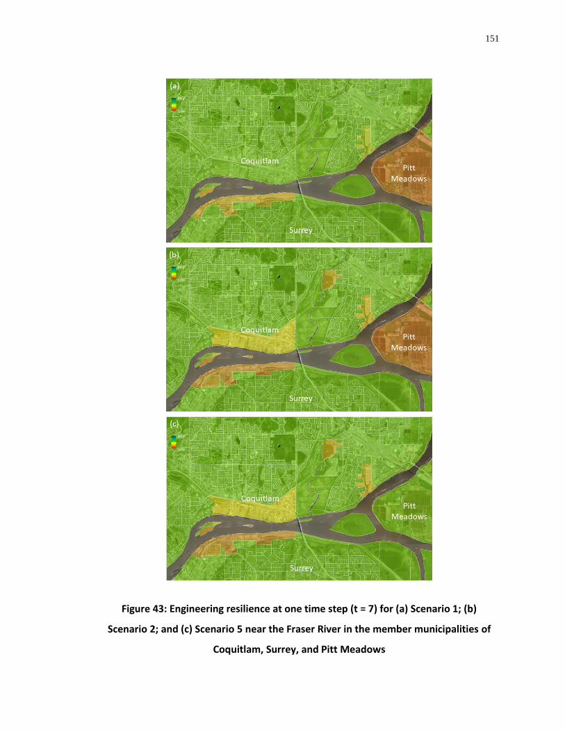
151
Figure 43: Engineering resilience at one time step (t = 7) for (a) Scenario 1; (b)
Scenario 2; and (c) Scenario 5 near the Fraser River in the member municipalities of
Coquitlam, Surrey, and Pitt Meadows
High
Low
High
Low
High
Low
152
The maps in Figure 44 provide an opportunity to see at the Regional level what is
happening to health resilience in space and time. These may be target locations to
implement adaptation options such as mobile health care (hospitals), raising roads, or to
target disaster emergency response and recovery operations. Taking a closer look at a few
of these areas, it can be seen that health resilience changes between simulation scenarios
for certain DAs. For many DAs in the City of Delta, health resilience in Scenarios 1, 2, and
3 is low due to the inundation of local roads, restricting access to hospitals. The closest
(non-auxiliary) hospitals are in neighbouring cities of Richmond, Surrey, and White Rock
(Figure 45). As roadways become inundated, the “cost” to get to hospitals increases and
system performance decreases. However, Scenario 4 represents the mobile hospital
adaptation option in which a mobile hospital is set up in the City of Delta to service the
area during a flood. So even though the DAs in Delta are subject to the same flooding
extent and depth as Scenario 2, the addition of a mobile health unit improves system
performance and resilience exceeds pre-shock levels (Figure 46).
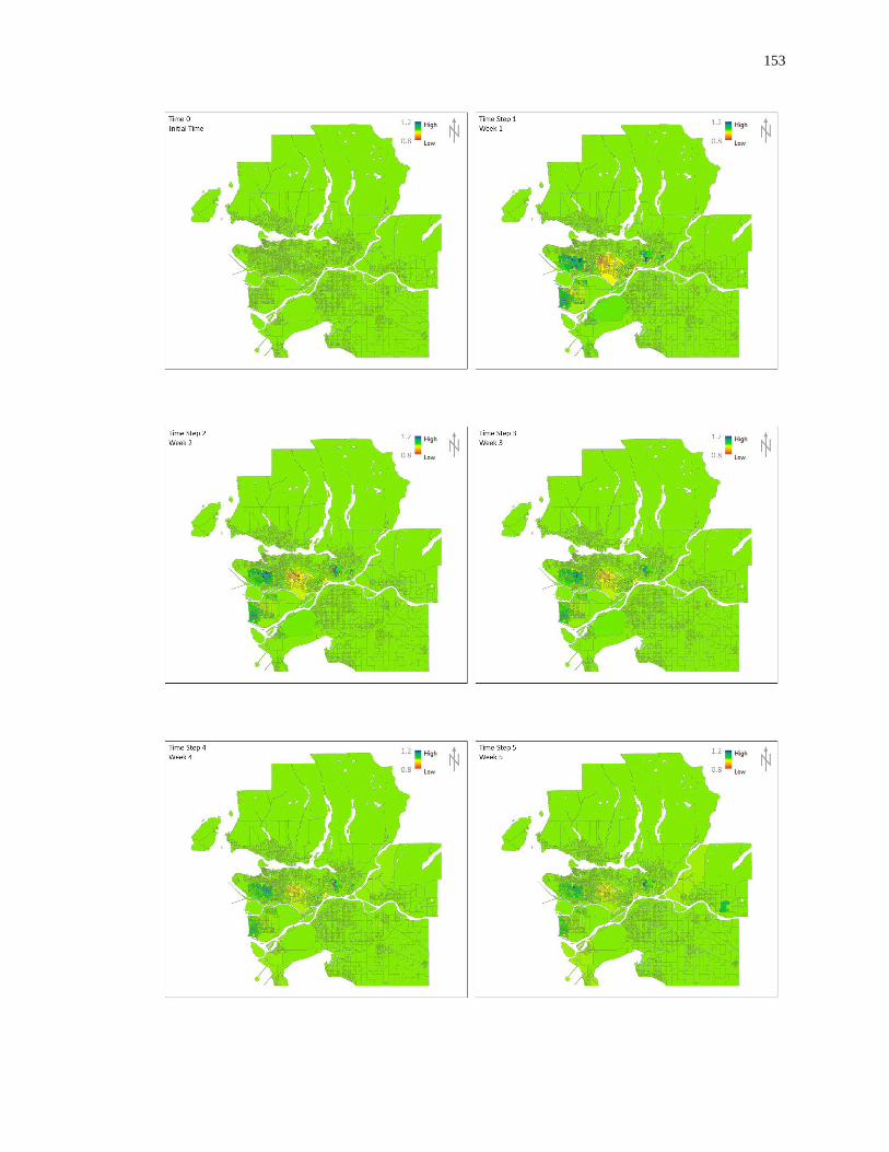
153
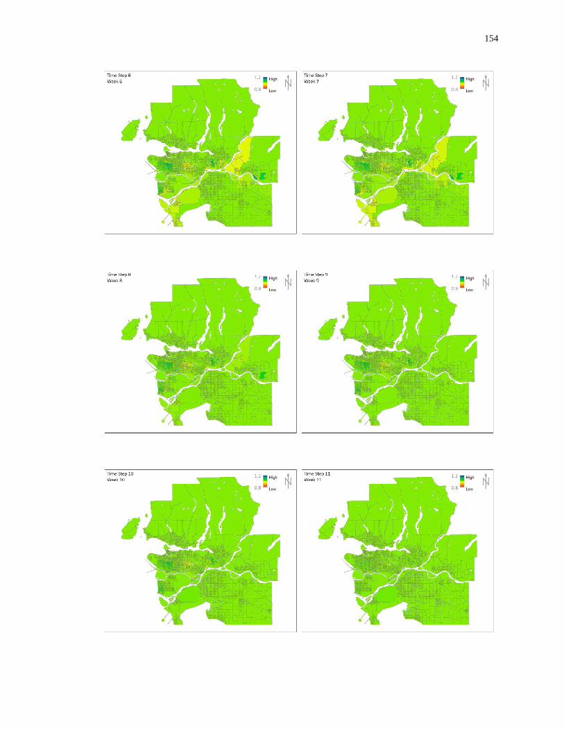
154
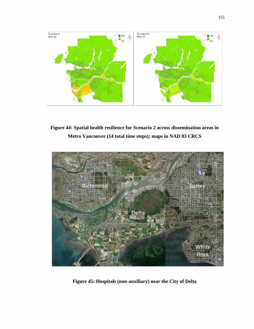
155
Figure 44: Spatial health resilience for Scenario 2 across dissemination areas in
Metro Vancouver (14 total time steps); maps in NAD 83 CRCS
Figure 45: Hospitals (non-auxiliary) near the City of Delta

156
Figure 46: Health resilience at one time step (t = 7) for (a) Scenario 1; (b) Scenario
2; and (c) Scenario 4 for the cities of Richmond, Delta, Surrey, and White Rock
High
Low
High
Low
High
Low
157
The maps in Figure 47 provide an opportunity to see at the Regional level what is
happening to social resilience in space and time. These may be target locations to
implement adaptation options such as backup emergency generators, mobile cell phone
stations, or something more drastic such as switching to alternative energy sources. The
social system yields particularly interesting results since its performance is network-based.
Spatially, this means that even service areas which are not directly inundated can be
impacted by the flood event. The spatial distribution in resilience values shown in the maps
in Figure 47 are driven by the algorithm currently implemented in the DRST, specifically
the iterative process of assigning cell phone users to operational (available) cell phone
towers. Taking a closer look at some of these areas, it can be seen that social resilience
changes over time and space for certain DAs. As flooded substations lose power, nearby
cell towers are impacted and also lose power. Subsequently, the remaining (powered) cell
towers iteratively pick up the unserved customers from the impacted DAs. The capacity of
each cell tower limits how many additional customers can be picked up from the impacted
area. As Figure 48 demonstrates, not all of the impacted areas are able to be serviced by
the remaining towers. This has an impact on social system performance, and subsequently
system resilience, since the social resilience indicator was defined as connectivity and its
metric of system performance is represented as people serviced.
What’s also interesting to note is that although the Regional scale was selected as the focal
scale for this application, it’s possible that if power were to be supplied from sources
outside of the Region, impacts may still be present at the Regional-level. Oftentimes system
impacts are not constrained within jurisdictional boundaries, which emphasizes the
importance of capturing cross-scale resilience; influences from above, and below, the focal
scale.
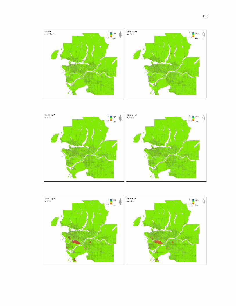
158
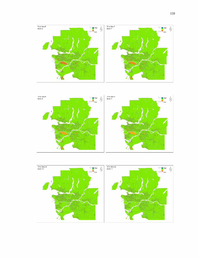
159

160
Figure 47: Spatial social resilience for Scenario 2 across dissemination areas in
Metro Vancouver (14 total time steps); maps in NAD 83 CRCS

161
Figure 48: Difference in social system impacts for one time step (t = 4) for
(a) Scenario 1; and (b) Scenario 2
162
5.5.2 Temporal Representation of Resilience
Maps are useful tools in the spatial representation of disaster resilience and the map set
(time series of maps) can provide insight into these spatial changes over time. However,
when considering the focal (Regional) scale of resilience assessment, it’s useful to look at
the simulation output graphs. These can provide insight into temporal dynamics of disaster
resilience and provide a convenient mechanism for scenario comparison.
Figure 49 shows temporal engineering resilience results for three (3) climate scenarios and
one (1) adaptation scenario. Everything else being equal, climate change has an impact on
Regional engineering resilience. As expected, resilience is lowest in Scenario 2, Scenario 1
is the highest, and Scenario 3 slightly outperforms Scenario 2. When considering the
emergency funding adaptation option (Scenario 6), it can be seen that declaring a state of
emergency and getting access to additional resources, results in higher resilience; system
performance is equally impacted by flooding (the disturbance), but the additional funding
allows the system to recover faster. This funding availability is driven by threshold
behaviour. This threshold is a gaming variable in the simulation and can be modified at the
beginning of a simulation to determine the impacts that the funding threshold has on
resilience.

163
Figure 49: Engineering resilience (Metro Vancouver)
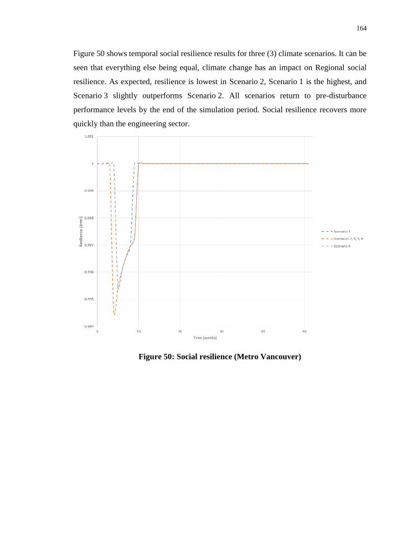
164
Figure 50 shows temporal social resilience results for three (3) climate scenarios. It can be
seen that everything else being equal, climate change has an impact on Regional social
resilience. As expected, resilience is lowest in Scenario 2, Scenario 1 is the highest, and
Scenario 3 slightly outperforms Scenario 2. All scenarios return to pre-disturbance
performance levels by the end of the simulation period. Social resilience recovers more
quickly than the engineering sector.
Figure 50: Social resilience (Metro Vancouver)

165
Figure 51 shows temporal health resilience results for three (3) climate scenarios and one
(1) adaptation option. It can be seen that everything else being equal, climate change has
an impact on Regional health resilience. As expected, resilience is lowest in Scenario 2,
Scenario 1 is the highest, and Scenario 3 slightly outperforms Scenario 2. When
considering the mobile hospital adaptation option (Scenario 4), it can be seen that the
addition of a mobile hospital station results in higher overall resilience; system
performance (and subsequently resilience) jumps higher since the addition of a temporary
hospital service occurs before the peak of the flood. The time and location of the mobile
hospital service was pre-determined and is unchangeable during the simulation, however
with slight modification to the DRST, the timing, location, and number of mobile stations
could all be adjusted to reflect any number of additional options.
Figure 51: Health resilience (Metro Vancouver)

166
Figure 52 shows temporal economic resilience results for three (3) climate scenarios and
three (3) adaptation options. It can be seen that everything else being equal, climate change
has an impact on Regional economic resilience. As expected, resilience is lowest in the
Scenario 2, Scenario 1 is the highest, and Scenario 3 slightly outperforms Scenario 2.
When considering any of the three (3) adaptation options, it can be seen that they do not
significantly impact economic resilience. Over the course of the one (1) year simulation
period, the economic resilience remains below a value of 1.0, indicating resilience has not
returned to pre-shock state. At the end of the simulation, they do not show any signs of
recovery, however this interpretation of these results could be a little misleading; provided
a longer simulation period, the resilience values actually begin increasing, approaching,
and even surpassing a value of 1.0 (Figure 53). The reasons for this behaviour is in part
due to the implementation of the economics domain in the DRST, operating as an
optimization model.
Figure 52: Economic resilience (Metro Vancouver)
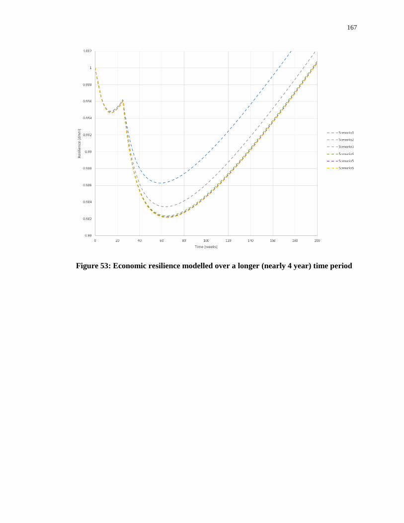
167
Figure 53: Economic resilience modelled over a longer (nearly 4 year) time period

168
Figure 54 shows temporal total resilience results for three (3) climate scenarios and three
(3) adaptation options. It can be seen that everything else being equal, climate change has
an impact on Regional total resilience. When comparing the three (3) climate change
scenarios (Scenario 1, Scenario 2, and Scenario 3) as expected, resilience is highest in
Scenario 1; lowest in Scenario 2; and Scenario 3 slightly outperforms Scenario 2. This is
because the climate-change influenced hydrometeorological hazards are influencing
system performance across all of the resilience domains.
When considering the three (3) adaptation options, (retreat, mobile hospital, and funding),
it can be seen that all of the adaptation options contribute to higher levels of overall
resilience, however Scenario 4 (mobile hospital) outperforms the other adaptation options.
Scenario 5 (managed retreat) does not significantly impact the overall resilience
calculation, as its total resilience is only marginally higher than Scenario 2.
Figure 54: Total resilience (Metro Vancouver)

169
Overall, the simulated change in resilience values is relatively low; the entire range of
resilience values fluctuates only within the range of 0.994 and 1.01. This is because
resilience, as per equation (3.3), is a function of the initial system performance. Since the
focal scale for resilience was established as the Metro Vancouver (regional) level, the
initial system performance is a function of the entire regional system. Therefore,
engineering performance at the regional level is described by the impacts to the entire
regional-scale building stock. Similarly, social resilience is a function of the impacts and
capacity of the entire regional population, health resilience is a function of the impacts and
capacity of region-wide access to healthcare facilities, and economic resilience is a function
of the regional economy. The impact of flooding on individual DAs can be significant as
observed in the maps presented in Figure 42, Figure 44, and Figure 47. However, this
resolution is lost when only evaluating resilience at the Regional level. As the spatio-
temporal maps in this chapter illustrate, resilience changes rather significantly at the DA
level. This stresses the importance of selecting a meaningful focal scale for resilience
assessment. The focal scale will drive the resolution of the resilience assessment and
conclusions.
Ultimately, the results suggest that overall Metro Vancouver is relatively resilient to
particular climate change influenced hydrometeorological disasters. However, particular
care should be exercised in the interpretation of these results since resilience is not evenly
distributed across the Region. Dissemination areas in the City of Richmond and Delta are
generally less resilient than the rest of the Region.
5.6 Chapter Summary
An application of the resilience quantification framework and calculation methodology
was applied to the region of Metro Vancouver, BC, Canada. First, the resilience landscape
was set and disaster resilience was characterized. Data was collected and a simulation
model was built to reflect four (4) important resilience domains. A single metric was
selected to represent system performance for each of the four (4) domains (engineering,
social, health, economy). Six (6) simulation scenarios (considering 3 climate change-based
scenarios and 3 adaptation options) were developed and run as part of proof-of-concept
implementation of the DRST. Adaptation options tested systems response and recovery

170
performance to shocks (hazard events). From the output maps and graphs, it can be seen
that climate change impacts disaster resilience and that various adaptation options can be
implemented to mitigate impacts and improve disaster resilience. The resilience framework
is intended to support disaster resilience quantification and aid in the development of
resilience-based assessment tools. The DRST is at the proof-of-concept stage and therefore
does not provide sufficient level of detail or ground-truthing to make it an appropriate tool
for real-world decision making. However with improvements, future iterations of the
DRST can be used by emergency management professionals and decision makers to
provide insight into the following key questions:
1. How are climate change influenced hydrometeorological hazards affecting
Metro Vancouver?
2. How can municipalities in Metro Vancouver better plan for, and adapt to, future
climate change-influenced hydrometeorological hazards?
3. How resilient is Metro Vancouver to climate change influenced
hydrometeorological hazards?
The following is an example of how the implementation of the disaster resilience quantification
framework and proof-of-concept DRST would be used to respond to the above questions:
How are climate change influenced hydrometeorological hazards affecting Metro
Vancouver?
Increasing temperatures and changes in precipitation are two of the main climatic drivers
of changes in water resources systems. Future changes are strongly linked to warming
trends and the seasonality and magnitude of river flows. A warming climate with increased
precipitation variability will likely increase exposure to sea level rise and riverine flooding
in Metro Vancouver. This is consistent with the sea level rise projections in Agam (2014)
and results of climate change influenced riverine flooding as presented in this dissertation.
How can municipalities in Metro Vancouver better plan for, and adapt to, future climate
change-influenced hydrometeorological hazards?

171
Climate change influenced sea level rise and riverine flooding will continue to threaten
coastal communities. With the pressures of increasing urbanization, development, and
unique hydrometeorological hazards, coastal communities need to better plan, prepare, and
respond to disasters. As a coastal city, Metro Vancouver can become more resilient to
climate change influenced hydrometeorological disasters by implementing adaptation
measures that will improve the robustness, redundancy, rapidity, and resourcefulness of
key disaster management-related city systems. Two (2) adaptation options which could
improve the resilience of Metro Vancouver are: enabling mobile treatment centres during
a disaster and access to additional financial resources. Managed retreat, as implemented
for a single DA in Pitt Meadows, does not contribute significantly to the overall resilience
of Metro Vancouver. One (1) adaptation option which could improve the resilience of Pitt
Meadows (municipality within Metro Vancouver) is managed retreat. Overall, managed
retreat could also prove to be an effective measure for increasing disaster resilience at the
Metro Vancouver level, however it would need to be implemented at a much larger scale
for multiple DAs along the Fraser River.
How resilient is Metro Vancouver to climate change influenced hydrometeorological
hazards?
Results suggest that Metro Vancouver exhibits a high degree of resilience at the Regional
scale. However, this resilience is not distributed proportionately across the Region. In some
DAs bordering the Fraser River, resilience drops nearly 20% in Scenario 2. This
demonstrates the importance in selecting an appropriate focal scale for resilience
assessment. To capture a holistic representation of disaster resilience, it is necessary to
consider the influence across multiple scales. However, resilience is both relative and
contextual and therefore selection of the focal scale will ultimately shape the assessment.
Careful consideration should be paid to the selection of the focal scale when establishing
research objectives, so that meaningful answers can be derived through the disaster
resilience assessment process.
172
Chapter 6
6 CONCLUSIONS
This chapter summaries the methodology, main findings and contributions of the research.
It also identifies some of the shortcomings of the resilience quantification methodology
and its application to Metro Vancouver. Since the DRST was a pioneering effort in
dynamic disaster resilience quantification, this chapter concludes with a discussion of
possible modifications, extensions and other sets of recommendations for future work in
the field of disaster management.
6.1 Summary of Methodology and Contributions to the Disaster Management Research Field
As described in Chapter 2, the climate is changing which will have significant impacts on
the magnitude, frequency, and seasonality of hazards across the globe. It is anticipated that
coastal megacities will be disproportionally affected by disasters in the future due to non-
climatic factors such as urbanization and rapid population growth in combination with
climatic factors such as increased exposure to climate change influenced
hydrometeorological hazards including sea level rise and riverine flooding. Therefore,
reducing the impacts of climate change-influenced hydrometeorological hazards on coastal
cities was identified as the primary motivation for pursuing the research in this dissertation.
To assess the current state of affairs, a review of existing disaster resilience definitions,
quantification techniques, and assessment tools was presented in Section 2.3. The
following is a summary of the issues and gaps identified in the review of resilience
literature and resilience practice, and a description of how these gaps were addressed as
part of this dissertation:
Issue 1: There is a growing recognition that resilience is temporally and spatially
dynamic, however improvements are still needed to explicitly account for spatio-
temporal dynamics in resilience quantification.
Chapter 3 presented a definition, methodological framework, and quantification method
for disaster resilience assessment that is dynamic in both time and space and which enables
173
the integration of multiple disaster resilience domains to provide a comprehensive
description of disaster resilience (additional work published in Simonovic and Peck, 2013).
This quantification method provides the ability to capture system improvements in the
process of recovery (i.e. recovery levels exceeding pre-disaster levels). This is considered
to be one of the key theoretical contributions of the work described in this dissertation.
Issue 2: Most existing resilience tools fail to identify thresholds as a significant
contributor to the expression and assessment of dynamic disaster resilience and
provide no means for its explicit inclusion in resilience quantification.
The dynamic resilience quantification expression and method presented in Chapter 3,
Section 3.2.2 and the work of Simonovic and Peck (2013), was expanded conceptually and
computationally to include dynamic disaster resilience quantification considering
thresholds, which is described in Chapter 3, Section 3.2.3. This is considered to be one of
the key theoretical contributions of the work described in this dissertation.
Issue 3: Improvements are still needed to explicitly quantitatively account for spatio-
temporal dynamics in resilience assessment tools.
Disaster resilience is dynamic in time and space. Chapter 4 describes the implementation
of the quantitative dynamic disaster resilience assessment methodology. A simulation tool
was developed called the Disaster Resilience Simulation Tool (DRST) to provide for
spatio-temporal dynamic disaster resilience assessment. It achieves this through the
integration of system dynamics simulation, economic optimization, and geographic
information systems (GIS) tools to account for complex, dynamic system interactions in
the quantification of dynamic spatio-temporal resilience. The DRST generates tables and
maps which can be used by disaster management professionals to identify where and when
to implement “resilience building” measures. The benefits of tight-coupling GIS and
system dynamics are published in a paper by the author in collaboration with others
(Neuwirth et al., (2015)). This paper provided the foundation for the development of the
DRST as presented in this dissertation. The DRST tool is considered to be one of the key
application contributions of the work described in this dissertation to the field of disaster
management.

174
6.2 Scope, Limitations, and Uncertainty
The research and applications contained herein offers one novel approach towards the
dynamic expression and quantification of disaster resilience. As may be expected in any
pioneering effort, there are a myriad of assumptions and limitations in this work, which
can hopefully be addressed as part of future work. The following is a summary of some of
the key assumptions and limitations of the work presented in this dissertation, separated
into two (2) categories: key assumptions and limitations of the disaster resilience
quantification framework; and limitations in the application of the framework to Metro
Vancouver. Sources of potential errors and uncertainties are also described, primarily as it
relates to the implementation of dynamic resilience quantification in the Metro Vancouver
application.
Limitations in Disaster Resilience Quantification Framework
The quantification framework operates under the assumption that all systems maintain the
same identity that they began with. Though thresholds were discussed, there are currently
no methods proposed to accommodate systems which exhibit transformative behaviour if
a threshold is crossed. Resilience as described in this dissertation, is considered as a
systems’ ability and capacity to adapt and adjust to shocks, and quickly return to a
functioning state. Since this definition describes resilience in relation to the initial pre-
shock functionality of the system, no attempts were made to describe transformative system
behaviour as part of resilience assessment.
The metrics used to represent system resilience were based on stakeholder workshops and
a review of disaster resilience literature but would benefit from ground-truthing and
supporting evidence to confirm that the selected metrics are truly reflective of disaster
resilient systems.
Limitations in the Application of the Framework (Metro Vancouver proof-of-
concept)
The economics model as described in this research by Gertz (2015) is a valuable
contribution to the field of natural disaster economics, however the existing optimization

175
model does not properly account for iterative feedbacks between disaster resilience
domains. If this model were deconstructed and rebuilt as a system as part of the dynamic
simulation model, it would better be able to capture cross-domain relationships and system
thresholds. In addition, the economics domain is currently represented as an optimization
model, which operates to optimize system efficiencies in the various economic sectors.
However, optimization of the elements in complex systems can actually reduce a systems’
resilience to disturbances (Walker and Salt 2006). While not described any further in this
dissertation, it is important to acknowledge this limitation which could be especially
limiting for future work that considers resilience to multiple disturbances (shocks).
Hydrologic and hydraulic modelling limitations are inherent in the modelling algorithms,
input data, and assumptions which are further described in Appendix G. Good engineering
practice should ground-truth physical model parameters in the field. Although MFLNRO
provided representative cross sections and model parameters were drawn from reliable
engineering-based reports, no survey or ground truthing was completed as part of this
dissertation.
The disaster resilience domains for Metro Vancouver are for illustrative purposes and form
a proof-of-concept example. The expression of these domains remains underdeveloped and
future research is recommended to identify additional potential resilience indicators within
each of the disaster resilience domains. Furthermore, discussions with stakeholders
revealed the ecological domain may play a significant role in disaster resilience and should
be recognized and incorporated into future iterations of the Metro Vancouver DRST.
There remains limited operationalized research on domain capacities and what exactly
contributes to disaster resilient cities (or regions). What’s more, there are even fewer
disaster resilience narratives for Metro Vancouver. This was acknowledged early on in the
research process so a series of workshops was held between 2011 and 2015 with local
stakeholders to help identify key disaster resilience domains and potential thresholds was
held to address this limitation,. These stakeholder workshops successfully brought together
individuals from various domains and spurred meaningful discussions on social, political,

176
and infrastructure systems. Though there was valuable insight gained from these meetings,
significant work remains in properly identifying key systems and thresholds.
A system dynamics approach to modelling cities and their component subsystems, makes
the assumption of perfect mixing and homogeneity within system components and within
each spatial unit (resolution of these units depends on the particular resilience domain and
available data). For instance, spatial data as represented in the social resilience domain
requires population data at the Dissemination Area (DA) level. This population is assumed
to be uniformly distributed throughout the DA, so any description of the system at a finer
resolution is not possible. This assumption applies to all resilience domains, across any
number of system components. The use of Agent-Based Modelling (ABM) could resolve
some of these limitations as it would capture the heterogeneity between entities and the
structure of their interactions. However, ABMs are typically data intensive and face their
own set of challenges including: the definition of component interactions; high data
quantity requirements; high resolution, detailed data and; higher, sometimes prohibitive,
model build and simulation times which subsequently may require the use of
supercomputers.
Lastly, but perhaps most significantly, modelling and simulation is data intensive. The
availability and quality of data required to develop and run spatio-temporal simulations is
acknowledged as a serious limitation in this work. However, the author is of the belief that
it’s better to build simulation models based on a series of assumptions than to entirely
abandon the effort altogether. The DRST, as with any other simulation model, should be
considered a “living tool” which can continually be improved and updated to include new
data and reflect new attitudes as the resilience landscape evolves.
Sources of Potential Errors and Uncertainties
It’s also important to identify potential sources of errors and uncertainties to make more
informed and relevant decision making and minimize the potential for maladaptation. Since
this dissertation focused on developing a disaster resilience assessment framework and
methodology for implementation, it may be considered as part of the pioneering efforts in
disaster resilience quantification. Though this dissertation offers just one of multiple ways

177
in which resilience can be quantified, it was intended to lay the foundation for future work
in spatio-temporal dynamic disaster resilience assessment. Since the work presented in this
dissertation may be considered cutting edge, there are many sources of potential errors and
uncertainties which remain unresolved, including:
Future climate change emissions trajectories used in hazard modelling;
Uncertainties in the appropriateness of some of the data processing algorithms;
The degree to which resilience performance metrics reflect real-world capacities
and resilience;
Spatial accuracy and attribute classifications of GIS data;
Aggregation errors in incomplete temporal and spatial datasets; and
Future system changes in societal and political priorities that were used to derive
appropriate adaptation options and estimate funding mechanisms.
Complex issues (and subsequently complex systems) are often characterized by various
types and sources of uncertainties. Common way to approach uncertainties in practice,
include: sensitivity analyses and Monte Carlo simulations. Although neither of these
methods was employed as part of this work, future iterations of the DRST would benefit
from an explicit consideration and evaluation of uncertainties. Then the DRST can help
identify the most robust strategies that perform well over a range of simulation scenarios.
It is important to evaluate and communicate levels and sources of uncertainties so decision
makers can understand the implications on their decisions and facilitate improved decision
making. One way to help curb the impacts of uncertainty is by promoting adaptive capacity
which helps prepare organizations to cope with a range of potential impacts.
6.3 Recommendations for Future Research
The research in this dissertation has already inspired additional work. The STDRM and
generic resilience quantification model as provided in this dissertation was applied to
research by Srivastav and Simonovic (2014) to simulate dynamic resilience of a railway

178
exposed to flooding. The STDRM and dynamic resilience calculation inspired work by
Irwin et al. (2016) to develop ResilSIM decision support tool, as applied to a case study in
the City of London, ON. In 2016 the dynamic resilience description was expanded by
Simonovic and Arunkumar (2016) to be applied to the operation of dams and reservoirs.
Most recently, the STDRM and resilience calculation was applied to a multi-hazard
resilience model of interdependent infrastructure systems by Kong and Simonovic (2018),
Zhang et al. (2018a), Zhang et al. (2018b), Kong and Simonovic (2019), and Kong et al.
(2019).
Although it is evident that the STDRM and resilience calculation has already progressed
into research performed by others, there are many additional opportunities to improve and
advance the work presented in this dissertation. As such, this section further focuses on
four distinct sets of recommendations for future work: modifying the current DRST to
permit simulation of other types of hazards; extension of the current DRST to include
additional disaster impacts and domains; use of resilience modelling and simulation
outputs; and lastly, more general recommendations for disaster resilience assessment.
6.3.1 Refinement of the DRST
A few of the next logical steps in the refinement of the DRST include: ground-truthing
model assumptions; explicitly exploring model uncertainties; and evaluating the numerical
model. Although each one of those tasks is a significant undertaking, one of the benefits
provided by the DRST is that it’s relatively simple to modify model parameters and
flexibility was built into the middleware program to accept new input data, as it becomes
available. An additional benefit provided by the DRST is it can be used to improve
decision-making under uncertainty since it can be easily altered to represent various
modeling assumptions and simulation scenarios.
In addition, refinement of the DRST would be desirable to address research questions such
as: What are possible adaptation options for other hazards?
The DRST application in BC considered high-flow large-scale flood events. Modelling
low-peak, long-duration, high-volume events is recommended for future work as there may

179
be significant impacts from these types of events and systems are likely to respond
differently under these conditions.
Although BC is an area of high seismic activity, the impacts of seismic events on flood
protection structures (e.g. dike damages or failures) are not considered in the scope of this
work. However, a separate study by Golder Associates (2014) has estimated that damage
from large-scale flooding due to seismic activity could reach $50 billion (CAD). Within
delta areas in particular, there is a high likelihood of having coincidental high water and
earthquake loadings (Golder Associates, 2014). The DRST was developed for assessing
the impacts of climate change influenced riverine flooding and sea level rise. However, the
tool could be adapted for additional types of applications. This particular example would
require modification of the input hazard as well as a redefinition of resilience impacts to
include the consequences of earthquakes and tsunamis.
If possible, it would be ideal for the DRST to be extended to simulate the behavior of
multiple simultaneous hazards, or to run multiple hazards back-to-back and see the impacts
on resilience.
6.3.2 Extension of the DRST
The current version of the DRST should be extended to provide a more complete
representation of disaster resilience. An extension of the tool could help identify whether
there are sufficient levels of detail in resilience quantification to be able to accurately
capture the complexities of disaster resilience.
A more comprehensive definition of resilience impacts and capacities is required. This is
an ongoing process that could become more refined. The DRST could benefit from the
inclusion of environmental and biological impacts, which may have complex interactions
and an influence on human health. Going forward, the DRST should be considered a living
tool, constantly evolving to test new adaptation options which may change based on
political and organizational priorities. As technology changes and as the resilience
landscape changes, the model will require updating.

180
The impacts of estuarial flooding were not considered as part of this research, however
additional research could be pursued to identify the influence of estuary systems in: (i) the
definition of physical hazard, and (ii) to determine whether combined salt-freshwater
environments plays a significant role in flooding impacts and disaster resilience. To
achieve this would require a sophisticated understanding of estuary systems and how salt
water affects environmental and physical (built) systems.
6.3.3 Resilience Outputs
The output of simulations using the DRST – and resilience models in general – could be
used for more detailed disaster management decisions. For example, if simulation results
determined that building additional disaster shelters was the best option to increase disaster
resilience, the resilience maps could be used to identify the areas which may benefit most
from addition of new disaster resilience shelters. Locations with low disaster resilience
could be selected as candidates for building the new shelters. Furthermore, a disaster shelter
site suitability analysis could be completed using spatial analysis techniques similar to
those implemented in the DRST (spatial queries, attribute queries, and descriptive
statistics) to determine the best locations to construct disaster shelters.
6.3.4 Model Evolution
To address some of the limitations of the proposed resilience modelling approach and SD
model, a hybrid SD-ABM modelling method could be used to better describe some of the
resilience domains, capture systems which operate on the individual agent level, and offer
some beneficial trade-offs between these two modelling approaches. This could help
capture cross-scale interactions for a more holistic description of resilience.

181
References
Acosta, J. D., Towe, V. L., Chari, R., Uscher-Pines, L., Sellers, C., & Chandra, A. (2015).
The Hungrier Games: Disaster Resilience Skills for Youth [Toolkit]. Research ANd
Development (RAND) Corporation. Retrieved from https://www.rand.org/well-
being/community-health-and-environmental-policy/centers/resilience-in-
action/community-resilience-toolkits.html
Acosta, J. D., Chandra, A., Xenakis, L., Varda, D. M., Eros-Sarnyai, M., Eisenman, D., …
Sprong, S. (2015). Partnerships for Recovery Across The Sectors (PRACTIS) Toolkit
[Toolkit]. Research ANd Development (RAND) Corporation. Retrieved from
https://www.rand.org/well-being/community-health-and-environmental-
policy/centers/resilience-in-action/community-resilience-toolkits.html
Acosta, J. D., Chandra, A., Towe, V. L., Zhao, Y., & Lu, Y. (2016). ENGAGED Toolkit:
Improving the Role of Nongovernmental Organizations in Disaster Response and
Recovery [Toolkit]. Research ANd Development (RAND) Corporation. Retrieved
from https://www.rand.org/well-being/community-health-and-environmental-
policy/centers/resilience-in-action/community-resilience-toolkits.html
Adger, W. N. (2007). Ecological and social resilience. In G. Atkinson, S. Dietz, & E.
Neumayer (Eds.), Handbook of Sustainable Development (pp. 78–90). Cheltenham,
UK: Elgar.
Agam, N. Development of Inundation Maps for the Vancouver Coastline Incorporating the
Effects of Sea Level Rise and Extreme (2014). Electronic Thesis and Dissertation
Repository, 2613.
Ahman, S., & Simonovic, S. P. (2000). System dynamics modeling of reservoir operations
for flood management. Journal of Computing in Civil Engineering, 14(3), 190–198.
Akanda, A. S., & Hossain, F. (2012). The Climate-Hater-Health Nexus in Emerging
Megacities. Eos, 93(37), 353–354. https://doi.org/10.1029/2012EO370001
182
Andre, A., Glen, A., Good, J., Gutsell, J., Hayat, I., Kershaw, J., Miller, J., Nash, J., &
Relkoff, T. (2000). Vulnerability of the Cellular Telecommunication Network in the
Lower Mainland British Columbia. Geography 452, Advanced Issues in Geographical
Information Systems, Department of Geography, Simon Fraser University.
Anslow, F. (2017, January). BC On Track to Set New Temperature Record in 2016.
University of Victoria: Pacific Climate Impacts Consortium.
Armington, P. (1969) A Theory of Demand for Products Distinguished by Place of
Production, International Monetary Fund Staff Papers, XVI, 159-78.
Arnell, N., Liu, C., Compagnucci, R., Da Cunha, L., Hanaki, K., Howe, C., … Döll, P.
(2001). Hydrology and Water Resources. In J. J. McCarthy, O. F. Canziani, N. A.
Leary, D. J. Dokken, & K. S. White (Eds.), Climate Change 2001: Impacts,
Adaptation, and Vulnerability (pp. 191–234). New York, NY: Cambridge University
Press.
Atukorala, U., Hawson, H., Mylleville, B., & Williams, R. (2014). Seismic Design
Guidelines for Dikes, 2nd Edition. Squamish, BC: Ministry of Forests, Lands and
Natural Resource Operations (MFLNRO), British Columbia.
Aven, T. (2011). On Some Recent Definitions and Analysis Frameworks for Risk,
Vulnerability, and Resilience. Risk Analysis, 31(4), 515–522.
https://doi.org/10.1111/j.1539-6924.2010.01528.x
Ayyub, B. M. (2015). Practical Resilience Metrics for Planning, Design, and Decision
Making. ASCE-ASME Journal of Risk and Uncertainty in Engineering Systems, Part
A: Civil Engineering, 1(2). https://doi.org/10.1061/AJRUA6.0000826
Balica, S. F., Wright, N. G., & van der Meulen, F. (2012). A flood vulnerability index for
coastal cities and its use in assessing climate change impacts. Natural Hazards, 64(1),
73–105. https://doi.org/10.1007/s11069-012-0234-1

183
Bathiany, S., Notz, D., Mauritsen, T., Raedel, G., & Brovkin, V. (2016). On the Potential
for Abrupt Arctic Winter Sea Ice Loss. Journal of Climate, 29(7), 2703–2719.
https://doi.org/10.1175/JCLI-D-15-0466.1
Bennett, E. M., Cumming, G. S., & Peterson, G. D. (2005). A Systems Model Approach to
Determining Resilience Surrogates for Case Studies. Ecosystems, 8, 945–957.
https://doi.org/10.1007/s10021-005-0141-3
Bindoff, N., Willebrand, J., Artale, V., Cazenave, A., Gregory, J., Gulev, S., …
Unnikrishnan, A. (2007). Observations: Oceanic Climate Change and Sea Level. In
Climate Change 2007: The Physical Science Basis (pp. 385–432). Cambridge, U.K.:
Cambridge University Press.
British Columbia Ministry of Envrionment. (2016). Indicators of Climate Change for
British Columbia, 2016 Update.
Bruneau, M., Chang, S. E., Eguchi, R. T., Lee, G. C., O’Rourke, T. D., Reinhorn, A. M.,
… Von Winterfeldt, D. (2003). A Framework to Quantitatively Assess and Enhance
the Seismic Resilience of Communities. Earthquake Spectra, 19(4), 733–752.
https://doi.org/10.1193/1.1623497
Burn, D. H., & Whitfield, P. H. (2016). Changes in floods and flood regimes in Canada.
Canadian Water Resources Journal, 41(1–2), 139–150.
https://doi.org/10.1080/07011784.2015.1026844
Campbell, J. E., & Shin, M. (2011). Geospatial Analysis I: Vector Operations. In Essentials
of Geographic Information Science v. 1.0 (pp. 167–185). Irvington, NY.
Cann, K. F., Thomas, D. R., Salmon, R. L., Wyn-Jones, A. P., & Kay, D. (2013). Extreme
water-related weather events and waterborne disease. Epidemiology and Infection,
141(4), 671–686. https://doi.org/10.1017/S0950268812001653
CARE: Climate Change and Resilience Platform (CCRP). (2018). Resilience Marker
[Toolkit]. Retrieved from https://careclimatechange.org/cares-resilience-marker/

184
CARE: Climate Change and Resilience Platform (CCRP). (2018). Resilience Marker
Guidance note.
CARE: Climate Change and Resilience Platform (CCRP). (2018). Resilience Marker
Vetting Form.
Carrera, L., Standardi, G., Bosello, F., & Mysiak, J. (2015). Assessing direct and indirect
economic impacts of a flood event through the integration of spatial and computable
general equilibrium modelling. Environmental Modelling and Software, 63, 109–122.
https://doi.org/10.1016/j.envsoft.2014.09.016
Chemtob, C. M., Nakashima, J. P., & Hamada, R. S. (2002). Psychosocial intervention for
postdisaster trauma symptoms in elementary school children: A controlled
community field study. Archives of Pediatrics and Adolescent Medicine, 156(3), 211–
216. https://doi.org/10.1001/archpedi.156.3.211
Clinton, H. R. (2006). It takes a village. New York, NY: Simon & Schuster.
Cochrane, H. C. (1974). Social science perspectives on the coming San Francisco
earthquake:Economic impact, prediction, and reconstruction. Boulder, Colorado.
Cook, J., Nuccitelli, D., Green, S., Richardson, M., Winkler, B., Painting, R., … Skuce, A.
(2016). Quantifying the consensus on anthropogenic global warming in the scientific
literature. Environmental Research Letters, 8(2), 1–7. https://doi.org/10.1088/1748-
9326/8/2/024024
Cutter, S. L., Barnes, L., Berry, M., Burton, C., Evans, E., Tate, E., & Webb, J. (2008). A
place-based model for understanding community resilience to natural disasters.
Global Environmental Change, 18(4), 598–606.
Cutter, S., Ahearn, J., Amadei, B., Crawford, P., Eidee, E. A., Galloway, G. E., … Zoback,
M. Lou. (2013). Disaster Resilience: A National Imperative. Environment: Science
and Policy for Sustainable Development, 55(2), 25–29.

185
Cutter, S. L. (2016). The landscape of disaster resilience indicators in the USA. Natural
Hazards, 80(2), 741–758. https://doi.org/10.1007/s11069-015-1993-2
Datar, A., Liu, J., Linnemayr, S., & Stecher, C. (2011). The Impact of Natural Disasters on
Child Health and Investments in Rural India. In Social Science and Medicine (Vol.
76).
de Bruijn, K., Buurman, J., Mens, M., Dahm, R., & Klijn, F. (2017). Resilience in practice:
Five principles to enable societies to cope with extreme weather events.
Environmental Science and Policy, 70, 21–30.
https://doi.org/https://doi.org/10.1016/j.envsci.2017.02.001
Dobbs, R., Remes, J., Manyika, J., Roxburgh, C., Smit, S., & Schaer, F. (2012). Urban
world: Cities and the rise of the consuming class. In McKinsey Global Institute.
Dunlap, D. (2017, April 4). Preparing for the Future Using Lessons From Hurricane Sandy.
New York Times.
Englum, L., & Grannis, J. (2017). Learning to Rebuild with Resilience. Retrieved October
17, 2018, from 100 Resilient Cities website: https://100resilientcities.org/learning-
build-resilience/
Environment Canada. (2013). Canada’s top ten weather stories of 2013. Retrieved January
5, 2019, from Environment and Climate Change Canada website:
http://www.ec.gc.ca/meteo-Weather/default.asp?lang=En&n=5BA5EAFC-
1&offset=3&toc=show
Environmental Systems Research Institute (ESRI). (2011). ArcGIS Desktop version 10:
ArcMap. Redlands, CA, USA: Environmental Systems Research Institute.
Eum, H., Sredojevic, D., & Simonovic, S. P. (2010). Engineering Procedure for the Climate
Change Flood Risk Assessment in the Upper Thames River Basin. Journal of
Hydrologic Engineering, 16(7), 608–612. https://doi.org/10.1061/(asce)he.1943-
5584.0000346
186
Fan, L. (2013). Disaster as opportunity? Building back better in Aceh, Myanmar and Haiti.
In Humanitarian Policy Group (HPG) Working Paper. London: Overseas
Development Institute.
Federal Emergency Management Agency (FEMA). (1996). Guide for All-Hazard
Emergency Operations Planning. Washington, D.C.
Federal Emergency Management Agency (FEMA). (2018). National Flood Insurance
Program (NFIP) Community Rating System (CRS) Brochure. Washington, D.C.
Forrester, J. W. (2007). System dynamics-a personal view of the first fifty years. 22(2/3),
345–358. https://doi.org/10.1002/sdr
Forrester, J. W. (1969). Urban Dynamics. Cambridge, Massachusetts: Massachusetts
Institute of Technology (MIT) Press.
Frumkin, H. (Ed.). (2010). Environmental Health: From Global to Local (2nd ed.). San
Francisco, CA: John Wiley & Sons, Inc.
Gastélum, J. R., Valdés, J. B., & Stewart, S. (2010). A System Dynamics Model to Evaluate
Temporary Water Transfers in the Mexican Conchos Basin. Water Resource
Management, 24(7), 1285–1311.
General Algebraic Modeling System (GAMS) Development Corporation. (1987). General
Algebraic Modeling System (GAMS). Washington, D.C., USA.
Gertz, A. B., Davies, J. B., & Black, S. L. (2019). A CGE Framework for Modeling the
Economics of Flooding and Recovery in a Major Urban Area. Risk Analysis, 39(6),
1314–1341. https://doi.org/10.1111/risa.13285
Gertz, A. B., & Jim MacGee, S. (2015). On the Economics of Climate Change and its
Effects. The University of Western Ontario.
187
Gesch, D. B. (2009). Analysis of Lidar Elevation Data for Improved Identification and
Delineation of Lands Vulnerable to Sea-Level Rise. Journal of Coastal Research,
(Special Issue 53), 49–58. https://doi.org/10.2112/SI53-006.1
Global Nutrition Cluster. (2008). A Toolkit for Addressing Nutrition in Emergency
Situations. In IASC Global Nutrition Cluster, UNICEF. New York, NY.
Godschalk, D. R. (2003). Urban Hazard Mitigation: Creating Resilient Cities. Natural
Hazards Review, 4(3), 136–143. https://doi.org/10.1061/(asce)1527-
6988(2003)4:3(136)
Goldmann, E., & Galea, S. (2014). Mental Health Consequences of Disasters. Annual
Review of Public Health, 35, 169–183. https://doi.org/10.1146/annurev-publhealth-
032013-182435
Goldstein, B. E., Wessells, A. T., Lejano, R., & Butler, W. (2015). Narrating Resilience:
Transforming Urban Systems Through Collaborative Storytelling. Urban Studies,
52(7), 1285–1303. https://doi.org/10.1177/0042098013505653
Gopinath, G., Swetha, T. V., & Ashitha, M. K. (2014). Automated extraction of watershed
boundary and drainage network from SRTM and comparison with Survey of India
toposheet. Arabian Journal of Geosciences, 7, 2625–2632.
https://doi.org/10.1007/s12517-013-0919-0
Grannis, J., Arroyo, V., Hoverter, S., Goetz, M., Bennett, A., DeWeese, J., … Deas, M.
(2016). Rebuilding with Resilience: Lessons from the Rebuild by Design Competition
After Hurricane Sandy. Washington, D.C.: Georgetown Climate Center.
Grossmann, W. D., & Eberhardt, S. (1992). Geographical information systems and
dynamic modelling: Potentials of a new approach. The Annals of Regional Science,
26, 53–66. https://doi.org/10.1007/BF01581480
Guha, A., & Lawrence, G. A. (2013). Estuary Classification Revisited. 43, 1566–1571.
https://doi.org/10.1175/JPO-D-12-0129.1
188
Gupta, M., Velasquez, G., Nag, S., Panda, A., Kuberan, R., Hari, K., & Suryono, R. (2010).
Building back better for next time. Bangkok, Thailand: UNISDR Secretariat Asia and
Pacific.
Haimes, Y. Y. (2011). Responses to Terje Aven’s paper: On Some Recent Definitions and
Analysis Frameworks for Risk, Vulnerability, and Resilience. Risk Analysis, 31(5),
689–692. https://doi.org/10.1111/j.1539-6924.2011.01587.x
Hallegatte, S. (2008). An Adaptive Regional Input-Output Model and its Application to
the Assessment of the Economic Cost of Katrina. Risk Analysis, 28(3), 779–799.
https://doi.org/10.1111/j.1539-6924.2008.01046.x
Hamman, J. J., Nijssen, B., Bohn, T. J., Gergel, D. R., & Mao, Y. (2018). The Variable
Infiltration Capacity model version 5 (VIC-5): infrastructure improvements for new
applications and reproducibility. Geoscientific Model Development, 11, 3481–3496.
https://doi.org/10.5194/gmd-11-3481-2018
Hammond, M. J., Chen, A. S., Butler, D., Djordjevic, S., & Manojlovic, N. (2013). A
framework for flood impact assessment in urban areas. Floods: From Risk to
Opportunity, 41–47.
Henry, K. (2016). Reaching Resilience: CARE Bangladesh Strategy to Disaster Risk
Reduction and Climate Change Adaptation. Dhaka, Bangladesh: CARE Bangladesh.
Henstra, D. (2012). Toward the Climate-Resilient City: Extreme Weather and Urban
Climate Adaptation Policies in Two Canadian Provinces. Journal of Comparative
Policy Analysis: Research and Practice, 14(2), 175–194.
https://doi.org/10.1080/13876988.2012.665215
Heymann, D. (2016). Explanation of Terms. In Control of Communicable Diseases
Manual. https://doi.org/10.2105/CCDM.2745.156
Hinkel, J., Lincke, D., Vafeidis, A. T., Perrette, M., Nicholls, R. J., Tol, R. S. J., …
Levermann, A. (2014). Coastal flood damage and adaptation costs under 21st century
189
sea-level rise. Proceedings of the National Academy of Sciences, 111(9), 3292–3297.
https://doi.org/10.1073/pnas.1222469111
Holling, C. S. (1973). Resilience and Stability of Ecological Systems. Annual Review of
Ecology and Systematics, 4, 1–23.
https://doi.org/10.1146/annurev.es.04.110173.000245
Hosseini, S., Barker, K., & Ramirez-Marquez, J. E. (2016). A review of definitions and
measures of system resilience. Reliability Engineering and System Safety, 145, 47–
61. https://doi.org/10.1016/j.ress.2015.08.006
Infrastructure Canada. (2018). Climate Lens [Toolkit]. Retrieved from
https://www.infrastructure.gc.ca/pub/other-autre/cl-occ-eng.html
Infrastructure Canada. (2018). Climate Lens General Guidance Version 1.1. Retrieved
from https://www.infrastructure.gc.ca/alt-format/pdf/guidelines-lignes-
directrices/climate-lens-general-guidance-2018-05-28.pdf
Inter-Agency Standing Committee (IASC). (2008). Nutrition Cluster A Toolkit for
Addressing Nutrition in Emergency Situations. Nutrition, (June).
Intergovernmental Panel on Climate Change (IPCC). (2014). Climate Change 2014:
Impacts, Adaptation, and Vulnerability. Part A: Global and Sectoral Aspects.
Contribution of Working Group II to the Fifth Assessment Report of the
Intergovernmental Panel on Climate Change (C. . Field, V. R. Barros, D. J. Dokken,
K. J. Mach, M. D. Mastrandrea, T. E. Bilir, … L. L. White, Eds.). Cambridge, United
Kingdom and New York, NY, USA: Cambridge University Press.
Intergovernmental Panel on Climate Change (IPCC). (2013). Climate Change 2013: The
Physical Science Basis. Contribution of Working Group I to the Fifth Assessment
Report of the Intergovernmental Panel on Climate Change (T. F. Stocker, D. Qin, G.-
K. Plattner, M. Tignor, S. K. Allen, J. Boschung, … P. M. Midgley, Eds.). Cambridge,
United Kingdom and New York, NY, USA: Cambridge University Press.
190
Intergovernmental Panel on Climate Change (IPCC). (2000). Special Report on Emissions
Scenarios: A Special Report of Working Group III of the Intergovernmental Panel on
Climate Change. New York, NY: Cambridge University Press.
Intergovernmental Panel on Climate Change (IPCC). (2014). Climate Change 2014:
Synthesis Report. Contribution of Working Groups I, II and III to the Fifth Assessment
Report of the Intergovernmental Panel on Climate Change (Core Writing Team, R.
K. Pachauri, & L. A. Meyer, Eds.). Geneva, Switzerland: IPCC.
Intergovernmental Panel on Climate Change (IPCC). (2007). Climate Change 2007:
Synthesis Report. Contribution of Working Groups I, II and III to the Fourth
Assessment Report of the Intergovernmental Panel on Climate Change (Core writing
team, R. . Pachauri, & A. Reisinger, Eds.). Geneva, Switzerland: IPCC.
Intergovernmental Panel on Climate Change (IPCC). (2012). Managing the Risks of
Extreme Events and Disasters to Advance Climate Change Adaptation. A Special
Report of Working Groups I and II of the Intergovernmental Panel on Climate Change
(C. B. Field, V. Barros, T. F. Stocker, D. Qin, D. J. Dokken, K. L. Ebi, … P. M.
Midgley, Eds.). Cambridge, UK and New York, NY, USA: Cambridge University
Press.
Intergovernmental Panel on Climate Change (IPCC). (2018). Global warming of 1.5°C. An
IPCC Special Report on the impacts of global warming of 1.5°C above pre-industrial
levels and related global greenhouse gas emission pathways, in the context of
strengthening the global response to the threat of climate change (V. Masson-
Delmotte, P. Zhai, H. O. Pörtner, D. Roberts, J. Skea, P. R. Shukla, … T. Waterfield,
Eds.). In Press: IPCC.
Irwin, S., Schardong, A., Simonovic, S. P., & Nirupama, N. (2016). ResilSIM-A Decision
Support Tool for Estimating Resilience of Urban Systems. Water, 8(9), 377.
https://doi.org/10.3390/w8090377

191
Jevrejeva, S., Jackson, L. P., Riva, R. E. M., Grinsted, A., & Moore, J. C. (2016). Coastal
sea level rise with warming above 2 °C. Proceedings of the National Academy of
Sciences, 113(47), 13342–13347. https://doi.org/10.1073/pnas.1605312113
Joerin, J., Shaw, R., Takeuchi, Y., & Krishnamurthy, R. (2012). Assessing community
resilience to climate-related disasters in Chennai, India. International Journal of
Disaster Risk Reduction, 1, 44–54. https://doi.org/10.1016/j.ijdrr.2012.05.006
Jones, E., & Faas, A. J. (Eds.). (2016). Social Network Analysis of Disaster Response,
Recovery, and Adaptation. Oxford, UK and Cambridge, MA, USA: Butterworth-
Heinemann.
Keim, M. E. (2008). Building Human Resilience: The Role of Public Health Preparedness
and Response As an Adaptation to Climate Change. American Journal of Preventive
Medicine, 35(5), 508–516. https://doi.org/10.1016/j.amepre.2008.08.022
Kelman, I. (2015). Climate Change and the Sendai Framework for Disaster Risk
Reduction. International Journal of Disaster Risk Science, 6, 117–127.
https://doi.org/10.1007/s13753-015-0046-5
Kerle, N., & Müller, A. (2013). Megacities and Natural Hazards. In P. T. Bobrowsky (Ed.),
Geographic Information Systems (GIS) and Natural Hazards (pp. 660–664).
https://doi.org/10.1007/978-1-4020-4399-4_231
Kerr Wood Leidal Associates (KWA) Ltd. (2011). Coastal Flood Mapping Guidelines and
Specifications, Final Report. Surrey, BC: Ministry of Forests, Lands & Natural
Reosurce Operations.
Kesavan, P. C., & Swaminathan, M. S. (2006). Managing extreme natural disasters in
coastal areas. Philosophical Transactions of the Royal Society A: Mathematical,
Physical and Engineering Sciences, 364, 2191–2216.
https://doi.org/10.1098/rsta.2006.1822

192
Khan, S., Yufeng, L., & Ahmad, A. (2009). Analysing complex behaviour of hydrological
systems through a system dynamics approach. Environmental Modelling and
Software, 24, 1363–1372. https://doi.org/10.1016/j.envsoft.2007.06.006
Khyrina, A. F. A. S., Burairah, H., & Abd Samad, H. B. (2012). A Systems Thinking in
Natural Disaster Management: Evacuation Preparedness. Advances in Economics,
Risk Management, Political and Law Science, 384–389.
Kjeldsen, T. R., & Rosbjerg, D. (2004). Choice of reliability, resilience and vulnerability
estimators for risk assessments of water resources systems. Hydrological Sciences
Journal, 49(5), 755–767. https://doi.org/10.1623/hysj.49.5.755.55136
Klise, K. A., Moriarty, D., Bynum, M. L., Murray, R., Burkhardt, J., & Haxton, T. M.
(2019). Water Network Tool for Resilience (WNTR) User Manual (EPA/600/R-
17/264). Washington, D.C.: US Environmental Protection Agency.
Kong, J., & Simonovic, S. P. (2018). A model of interdependent infrastructure system
resilience. International Journal of Safety and Security Engineering, 8(3), 377–389.
https://doi.org/10.2495/SAFE-V8-N3-377-389
Kong, J., Simonovic, S. P., & Zhang, C. (2019). Sequential Hazards Resilience of
Interdependent Infrastructure System: A Case Study of Greater Toronto Area Energy
Infrastructure System. Risk Analysis, 39(5), 1141–1168.
https://doi.org/10.1111/risa.13222
Kong, J., & Simonovic, S. P. (2019). Probabilistic Multiple Hazard Resilience Model of
an Interdependent Infrastructure System. Risk Analysis : An Official Publication of
the Society for Risk Analysis, Risk Analysis. https://doi.org/10.1111/risa.13305
Kreibich, H., & Bubeck, P. (2013). Natural Hazards: Direct Costs and Losses Due to the
Disruption of Production Processes. In Global Assessment Report on Disaster Risk
Reduction 2015. Postdam, Germany.

193
Kuzņecova, T., & Romagnoli, F. (2014). System Dynamics approach within the context of
city resilience and urban metabolism. 9th International Conference “Environmental
Engineering.” Vilnius, Lithuania.
Lentz, E. E., Thieler, E. R., Plant, N. G., Stippa, S. R., Horton, R. M., & Gesch, D. B.
(2016). Evaluation of dynamic coastal response to sea-level rise modifies inundation
likelihood. Nature Climate Change, 6, 696–700. https://doi.org/10.1038/nclimate295
Liang, X., Lettenmaier, D. P., Wood, E. F., & Burges, S. J. (1994). A simple hydrologically
based model of land surface water and energy fluxes for general circulation models.
Journal of Geophysical Research, 99(D7), 14415–14428.
https://doi.org/10.1029/94JD00483
Lin, W., Chou, W., Lin, C., Huang, P., & Tsai, J. (2005). Automated suitable drainage
network extraction from digital elevation models in Taiwan’s upstream watersheds.
Hydrological Processes, 20(2), 289–306.
Lohmann,D, Raschke, E., Nijssen, B. & Lettenmaier, D.P. (1998). Regional scale
hydrology: I. Formulation of the VIC-2L model coupled to a routing model,
Hydrological Sciences Journal, 43:1, 131-141, DOI: 10.1080/02626669809492107
Luther, L. (2008). CRS Report for Congress, Disaster Debris Removal After Hurricane
Katrina: Status and Associated Issues. USA: Congressional Research Service.
Luther, L. (2011). CRS Report for Congress, Managing Disaster Debris: Overview of
Regulatory Requirements, Agency Roles, and Selected Challenges. USA:
Congressional Research Service.
Malilay, J., Henderson, A., McGeehin, M., & Flanders, W. D. (1997). Estimating Health
Risks from Natural Hazards Using Risk Assessment and Epidemiology. Risk Analysis,
17(3), 353–358. https://doi.org/10.1111/j.1539-6924.1997.tb00873.x
Masud, M. B., Soni, P., Shrestha, S., & Tripathi, N. K. (2016). Changes in Climate
Extremes over North Thailand, 1960–2099. Journal of Climatology, 1–18.
https://doi.org/10.1155/2016/4289454
194
McBean, G., & Rodgers, C. (2010). Climate hazards and disasters: the need for capacity
building. Wiley Interdisciplinary Reviews: Climate Change, 1(6), 871–884.
https://doi.org/10.1002/wcc.77
Metro Vancouver. (2017). About Us. Retrieved July 22, 2018, from
http://www.metrovancouver.org/about/Pages/default.aspx
Metro Vancouver. (2018). Climate 2050 Strategic Framework. Burnaby, BC: Metro
Vancouver.
Metro Vancouver. (2010). Corporate Climate Action Plan. Burnaby, BC: Metro
Vancouver.
Ministry of Forests Lands Natural Resource Operations (MFLNRO). (2014). Fraser River
Design Flood Level Update - Hope to Mission, Final Report. Surrey, BC.
Nan, C., & Sansavini, G. (2017). A quantitative method for assessing resilience of
interdependent infrastructures. Reliability Engineering and System Safety, 157, 35–
53. https://doi.org/10.1016/j.ress.2016.08.013
Nastev, M., & Todorov, N. (2013). Hazus: A standardized methodology for flood risk
assessment in Canada. Canadian Water Resources Journal, 38(3), 223–231.
https://doi.org/10.1080/07011784.2013.801599
National Aeronautics and Space Administration (NASA) Jet Propulsion Laboratory:
California Institute of Technology. (2015). NASA Holds Media Briefing on Carbon’s
Role in Earth’s Future Climate. Retrieved March 8, 2019, from
www.jpl.nasa.gov/news/news.php?feature=4749
National Aeronautics and Space Administration (NASA) Jet Propulsion Laboratory:
California Institute of Technology. (2009). Global Climate Change Vital Signs of the
Planet: The Causes of Climate Change. Retrieved June 17, 2019, from
https://climate.nasa.gov/causes/
195
National Oceanic and Atmospheric Administration (NOAA). (2017). Detailed Method for
Mapping Sea Level Rise Inundation. Office for Coastal Management: National
Oceanic and Atmospheric Administration.
Nelson, D. R., Adger, W. N., & Brown, K. (2007). Adaptation to Environmental Change:
Contributions of a Resilience Framework. Annual Review of Environment and
Resources, 32, 395–419. https://doi.org/10.1146/annurev.energy.32.051807.090348
Neuwirth, C., Peck, A., & Simonović, S. P. (2015). Modeling structural change in spatial
system dynamics: A Daisyworld example. Environmental Modelling and Software,
65, 30–40. https://doi.org/10.1016/j.envsoft.2014.11.026
Norris, F. H., Stevens, S. P., Pfefferbaum, B., Wyche, K. F., & Pfefferbaum, R. L. (2008).
Community Resilience as a Metaphor, Theory, Set of Capacities, and Strategy for
Disaster Readiness. American Journal of Community Psychology, 41(1–2), 127–150.
https://doi.org/10.1007/s10464-007-9156-6
Northwest Hydraulic Consultants (NHC). (2008). Fraser River Hydraulic Model Update,
Final Report. Surrey, BC: Ministry of Envrionment.
O’Neill, H. K., McLean, A. J., Kalis, R., & Shultz, J. M. (2016). Disaster averted:
Community resilience in the face of a catastrophic flood. Disaster Health, 3(3), 67–
77. https://doi.org/10.1080/21665044.2016.1219575
Organisation for Economic Co-operation and Development (OECD). (2014). Guidelines
for Resilience Systems Analysis. OECD Publishing.
Orr, D. (2014). Systems Thinking and the Future of Cities. The Solutions Journal, 5(1),
54–61.
Pacific Climate Impacts Consortium (PCIC). (2014). Gridded Hydrologic Model Output.
Retrieved May 26, 2019, from http://www.pacificclimate.org/
196
Pant, R., Barker, K., & Zobel, C. (2014). Static and dynamic metrics of economic resilience
for interdependent infrastructure and industry sectors. Reliability Engineering &
System Safety, 125, 92–102.
Paton, D., & Johnston, D. (2006). Disaster Resilience: An Integrated Approach.
Springfield, Illinois, USA: Charles C Thomas Publishing Ltd.
Patz, J. A., Frumkin, H., Holloway, T., Vimont, D. J., & Haines, A. (2014). Climate
Change: Challenges and Opportunities for Global Health. Journal of the American
Medical Association, 312(15), 1565–1580. https://doi.org/10.1001/jama.2014.13186
Peacock, W.G., Brody, S., Seitz, W., Merrell, W., Vedlitz, A., Zahran, S., Harriss, R.,
Stickney, R., (2010). Advancing Resilience of Coastal Localities: Developing
Implementing, and Sustaining the Use of Coastal Resilience Indicators: A Final
Report. Hazard Reduction and Recovery Center.
Peck, A., Neuwirth, C., & Simonovic, S.P. (2014). Coupling System Dynamics with
Geographic Information Systems: CCaR Project Report Water Resources Research
Report no. 086, Facility for Intelligent Decision Support, Department of Civil and
Environmental Engineering, London, Ontario, Canada, 60 pages. ISBN: (print) 978-
0-7714-3069-5; (online) 978-0-7714-3070-1.
Peck, A. & Simonovic, S.P. (2013). Coastal Cities at Risk (CCaR): Generic System
Dynamics Simulation Models for Use with City Resilience Simulator. Water
Resources Research Report no. 083, Facility for Intelligent Decision Support,
Department of Civil and Environmental Engineering, London, Ontario, Canada, 55
pages. ISBN: (print) 978-0-7714-3024-4; (online) 978-0-7714-3025-1.
Pomeroy, J. W., Stewart, R. E., & Whitfield, P. H. (2015). The 2013 flood event in the
South Saskatchewan and Elk River basins: Causes, assessment and damages.
Canadian Water Resources Journal, 41(1–2), 105–117.
https://doi.org/10.1080/07011784.2015.1089190

197
Radić, V., & Hock, R. (2011). Regionally differentiated contribution of mountain glaciers
and ice caps to future sea-level rise. Nature Geoscience, 4, 91–94.
https://doi.org/10.1038/ngeo1052
Radzicki, M. J., & Robert, T. (1997). Introduction to System Dynamics: A systems
approach to understanding complex policy issues. United States Department of
Energy.
Ramezankhani, A., & Najafiyazdi, M. (2006). A System Dynamics Approach on Post-
Disaster Management: A Case Study of Bam Earthquake, December 2003.
Proceedings of the 26th International Conference of the System Dynamics Society.
Rose, A. (2017). Defining and Measuring Economic Resilience (Integrated). Singapore:
Springer.
Sanders, P., & Sanders, F. (2004). Spatial urban dynamics: a vision on the future of urban
dynamics. In Paper presented at the 22nd International Conference of the System
Dynamics Society. Oxford.
Schnorbus, M., Werner, A., & Bennett, K. (2014). Impacts of climate change in three
hydrologic regimes in British Columbia, Canada. Hydrological Processes, 28, 1170–
1189. https://doi.org/10.1002/hyp.9661
Sharifi, A. (2016). A critical review of selected tools for assessing community resilience.
Ecological Indicators, 69, 629–647. https://doi.org/10.1016/j.ecolind.2016.05.023
Sharma, D., & Babel, M. S. (2013). Application of downscaled precipitation for
hydrological climate-change impact assessment in the upper Ping River Basin of
Thailand. Climate Dynamics, 41(9–10), 2589–2602. https://doi.org/10.1007/s00382-
013-1788-7
Shaw, R., Takeuchi, Y., Joerin, J., Fernandez, G., 2010. Climate and Disaster Resilience
Initiative Capacity-Building Program. Kyoto University, Kyoto, Japan.
198
Shepherd, A., Wingham, D., Wallis, D., Giles, K., Laxon, S., & Sundal, A. V. (2010).
Recent loss of floating ice and the consequent sea level contribution. Geophysical
Research Letters, 37(13), 1–5. https://doi.org/10.1029/2010GL042496
Shrestha, R. R., Schnorbus, M. A., Werner, A. T., & Berland, A. J. (2012). Modelling
spatial and temporal variability of hydrologic impacts of climate change in the Fraser
River basin, British Columbia, Canada. Hydrological Processes, 26, 1840–1860.
https://doi.org/10.1002/hyp.9283
Shrestha, S. (2014). Assessment of water availability under climate change scenarios in
Thailand. In Climate Change Impacts and Adaptation in Water Resources and Water
Use Sectors (pp. 9–23). https://doi.org/10.1007/978-3-319-09746-6
Shrubsole, D., Brooks, G., Halliday, R., Haque, E., Kumar, A., Lacroix, J., … Simonovic,
S. P. (2003). An Assessment of Flood Risk Management in Canada. ICLR Research
Paper Series, No. 28, 71.
Siddiqi, Y., & Salem, M. (2012). A Social Accounting Matrix for Canada. Statistics
Canada, Analytical Studies Branch, Economic Analysis (EA) Research Paper Series,
2012.
Simonovic, S. (2009). Managing Water Resources: Methods and Tools for a Systems
Approach. Paris, France and London, UK: UNESCO Publishing.
Simonovic, S. P., & Peck, A. (2013). Dynamic Resilience to Climate Change Caused
Natural Disasters in Coastal Megacities Quantification Framework. British Journal of
Environment and Climate Change, 3(3), 378–401.
https://doi.org/10.9734/bjecc/2013/2504
Simonovic, S., & Arunkumar, R. (2016). Comparison of static and dynamic resilience for
a multipurpose reservoir operation. Water Resources Research, 5(3), 8630–8649.
https://doi.org/10.1002/ 2016WR019551

199
Simonovic, S., & Arunkumar, R. (2016). Comparison of static and dynamic resilience for
a multipurpose reservoir operation. Water Resources Research, 52(11), 8630–8649.
https://doi.org/https://doi.org/10.1002/2016WR019551
Simonovic, S. P., Irwin, S., & Schardong, A. (2016). Resilience simulation tool (ResilSIM)
[Toolkit]. London, ON. Retrieved from https://resilsim-uwo.ca/About
Srivastav, R., & Simonovic, S. P. (2014). Simulation of Dynamic Resilience : A Railway
Water Resources Research Report Simulation of Dynamic Resilience : A Railway
Case Study. London, ON: Western University.
Statistics Canada. (2018). Dissemination Area (DA): Plain Language Definition. Retrieved
November 22, 2018, from Statistics Canada Illustrated Glossary website:
https://www150.statcan.gc.ca/n1/pub/92-195-x/2011001/geo/da-ad/da-ad-eng.htm
Steinfeld, C. M. M., Kingsford, R. T., & Laffan, S. W. (2013). Semi-automated GIS
techniques for detecting floodplain earthworks. Hydrological Processes, 27, 579–591.
https://doi.org/10.1002/hyp.9244
Stenström, P. (2004). Hydraulics and mixing in the Hudson River estuary: A numerical
model study of tidal variations during neap tide conditions. Journal of Geophysical
Research: Oceans, 109(C4). https://doi.org/10.1029/2003JC001954
Towe, V. L., Chandra, A., Acosta, J. D., Chari, R., Uscher-Pines, L., & Sellers, C. (2015).
Community Resilience: Learn and Tell Toolkit [Toolkit]. Research ANd
Development (RAND) Corporation. Retrieved from https://www.rand.org/well-
being/community-health-and-environmental-policy/centers/resilience-in-
action/community-resilience-toolkits.html
United Nations (UN). (1997). United Nations Framework Convention on Climate Change
Chapter XXVII: Environment, Kyoto Protocol. Kyoto, Japan: United Nations.
United Nations (UN). (1992). United Nations Framework Convention on Climate Change
Treaty Chapter XXVII. Environment. New York, NY: United Nations.

200
United Nations Department of Economic and Social Affairs (UN DESA). (2018). Revision
of World Urbanization Prospects. Retrieved May 11, 2019, from United Nations
Department of Economic and Social Affairs website:
https://population.un.org/wup/Publications/
United Nations International Strategy for Disaster Reduction (UNISDR). (2005). Hyogo
Framework for Action 2005-2015: Building the Resilience of Nations and
Communities to Disasters. In Extracted from the final report of the World Conference
on Disaster Reduction (A/CONF.206/6). Geneva, Switzerland; Nairobi, Kenya and
Bangkok, Thailand.
UNDRR. (2017). Disaster Resilience Scorecard for Cities. The United Nations Office for
Disaster Reduction, (Version 2.2), 56.
United Nations Office for Disaster Risk Reduction (UNDRR). (2016). Report of the open-
ended intergovernmental expert working group on indicators and terminology
relating to disaster risk reduction (Vol. 71).
https://doi.org/https://www.preventionweb.net/files/50683_oiewgreportenglish.pdf
University of Western Ontario (UWO): Facility for Intelligent Decision Support. (2016).
About the ResilSIM tool. Retrieved January 4, 2019, from https://resilsim-
uwo.ca/About
US Army Corps of Engineers (USACE). (2011). HEC-GeoRAS: GIS Tools for Support of
HEC-RAS using ArcGIS, HEC-GEORAS User’s Manual version 4.3.93. Davis, CA,
USA: US Army Corp of Engineers Hydrologic Engineering Center.
US Army Corps of Engineers (USACE). (2010). HEC-RAS River Analysis System:
Hydraulic Reference Manual version 4.1. Davis, CA, USA: US Army Corp of
Engineers Hydrologic Engineering Center.
US Environmental Protection Agency. (2018). Water Network Tool for Resilience
(WNTR) [Toolkit]. Washington, D.C., USA. Retrieved from
201
https://cfpub.epa.gov/si/si_public_record_report.cfm?Lab=NHSRC&dirEntryId=337
793
Ventana Systems Inc. (2009). Vensim DSS. Massachusetts, USA.
Walker, B., & Salt, D. (2012). Resilience Practice: Building Capacity to Absorb
Disturbance and Maintain Function. Washington: Island Press.
Walker, B., & Salt, D. (2006). Resilience Thinking: Sustaining Ecosystems and People in
a Changing World. Washington, D.C.: Island Press.
Watson, J., Gayer, M., & Connolly, M. (2007). Epidemics after Natural Disasters.
Emerging Infectious Diseases, 13(1), 1–5.
Watters, J. (2014). Disaster Recovery, Crisis Response, and Business Continuity: A
Management Desk Reference. Berkeley: Apress.
Wenzel, F., Bendimerad, F., & Sinha, R. (2007). Megacities - megarisks. Natural Hazards,
42(3), 481–491. https://doi.org/10.1007/s11069-006-9073-2
Werner, A. T. (2011). BCSD Downscaled Transient Climate Projections for Eight Select
GCMS over British Columbia, Canada. Victoria, BC: Pacific Climate Impacts
Consortium, University of Victoria.
Wong, P. P., Losada, I. J., Gattuso, J.-P., Hinkel, J., Khattabi, A., McInnes, K. L., …
Sallenger, A. (2014). Coastal systems and low-lying areas. In C. B. Field, V. R.
Barros, D. J. Dokken, K. J. Mach, M. D. Mastrandrea, T. E. Bilir, … L. L. White
(Eds.), Climate Change 2014: Impacts, Adaptation, and Vulnerability. Part A: Global
and Sectoral Aspects. Contribution of Working Group II to the Fifth Assessment
Report of the Intergovernmental Panel on Climate Change (pp. 361–409).
Cambridge, United Kingdom and New York, NY, USA: Cambridge University Press.
World Health Organization (WHO). (2018). Drowning: Key facts.

202
World Health Organization (WHO). (2003). Climate change and human health: risk and
responses (A. J. McMichael, D. H. Campbell-Lendrum, C. F. Corvalán, K. L. Ebi, A.
K. Githeko, J. D. Scheraga, & A. Woodward, Eds.). Geneva, Switzerland.
World Health Organization (WHO). (2013). Building Back Better: Sustainable Mental
Health Care after Emergencies. Geneva, Switzerland: World Health Organization.
Xie, H., & Rao, R. (2014). A system dynamics model for medical staff allocation in post-
Wenchuan earthquake relief. Proceedings - 2014 IEEE Workshop on Advanced
Research and Technology in Industry Applications, WARTIA 2014, 307–311.
https://doi.org/10.1109/WARTIA.2014.6976258
Zeleňáková, M., Blišťan, P., Alkhalaf, I., Gaňová, L., & Zvijáková, L. (2016). Assessment
of environmental damages in case of flood in Bodva River basin, Slovakia.
International Journal of Safety and Security Engineering, 6(3), 498–507.
https://doi.org/10.2495/SAFE-V6-N3-498-507
Zhang, C., Kong, J., & Simonovic, S. P. (2018a). Restoration resource allocation model
for enhancing resilience of interdependent infrastructure systems. Safety Science, 102,
169–177. https://doi.org/10.1016/j.ssci.2017.10.014
Zhang, C., Kong, J., & Simonovic, S. P. (2018b). Modeling joint restoration strategies for
interdependent infrastructure systems. Public Library of Science (PLoS) ONE, 13(4),
18. https://doi.org/10.1371/journal.pone.0195727

203
Appendix A
An Introduction to Spatial Data, Spatial Data Tools, and their
use in the Development of the DRST
Spatial data and the representation of disaster resilience as dynamic in both time and space
required the acquisition, understanding, and use of various types and formats of spatial data
and data analysis tools. This Appendix provides a brief introduction to various types of
spatial data and describes the various formats of data used in the development of the
Disaster Resilience Simulation Tool. It covers the following topics:
- An introduction to spatial data;
- Spatial data types; and
- Spatial reference systems.
The various spatial data described in this Appendix was manipulated using several spatial
analysis tools. The following Appendix therefore also lists and describes the suite of spatial
analysis tools implemented in the Disaster Resilience Simulation Tool. These tools were
accessed via the ArcGIS dynamic link library (DLL) and implemented with the use of
Python scripts. Note that some of these tools are only available with an active ArcGIS
Spatial Analyst or Network Analyst License:
- Extract Tools (clip, select, split)
- Overlay Tools (union, intersect, erase)
- Proximity Tools (buffer, cost-distance)
- Reclass Tools (lookup, reclassify)
- Geometric Network Tools (create geometric network, set flow direction, trace
geometric network)
When the extract, overlay, proximity, and reclassify spatial tools are executed in a
sequence, it is referred to as geoprocessing. The DRST incorporates geoprocessing into its
preparation of spatial resilience inputs for various (economic, engineering, health, and
social) model domains. The DRST geoprocessing sequences are executed in a Python
middleware program.
204
An Introduction to Spatial Data: Spatial data is used to represent features in the real
world. Digitally, these pieces of data are organized and stored together as layers. There are
many different forms of spatial data including tables, shapefiles, markup files (such as
KML), etc. Although spatial data comes in many diverse formats (Table 8) it shares the
similar characteristic of being linked to a location which is typically defined by a set of
coordinates (latitude and longitude). With this location information, data can be mapped,
typically using geographic information system (GIS) software. Mapped data can then be
represented as thematic layers stacked on top of each other to gain a better understanding
of the spatial landscape and features at a particular location (Figure 55). Furthermore, the
spatial relationships between map features can be explored using spatial analysis
techniques.
To effectively organize spatial data, features are often grouped together in datasets and
spatially represented as layers. Map layers are thematic representations of different types
of geographic information which may include: discrete features, continuous surfaces,
object attributes, and imagery (Table 8). The DRST makes use of all of these types of data
in order to represent various features and phenomena in resilience calculations and, where
necessary, converts between these representations based on the intended use of the data.
This spatial data was essential for resilience mapping. The remainder of this section
identifies more specifically the key characteristics of spatial data, the preparations of spatial
data, and analysis of spatial data for use in the DRST.
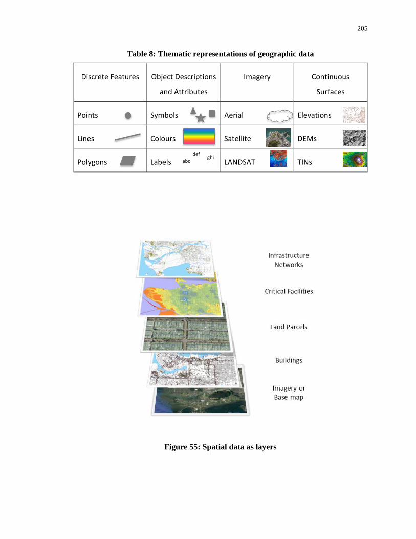
205
Table 8: Thematic representations of geographic data
Discrete Features Object Descriptions
and Attributes
Imagery Continuous
Surfaces
Points Symbols Aerial Elevations
Lines Colours Satellite DEMs
Polygons Labels LANDSAT TINs
Figure 55: Spatial data as layers
abc ghi def
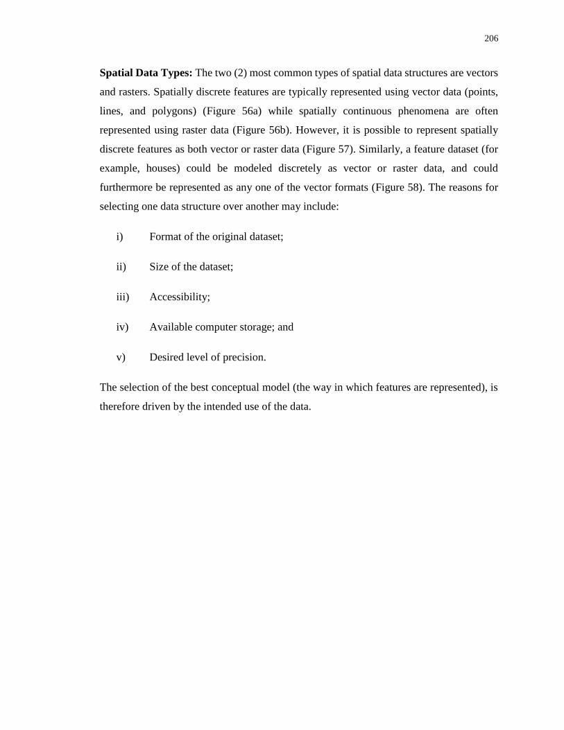
206
Spatial Data Types: The two (2) most common types of spatial data structures are vectors
and rasters. Spatially discrete features are typically represented using vector data (points,
lines, and polygons) (Figure 56a) while spatially continuous phenomena are often
represented using raster data (Figure 56b). However, it is possible to represent spatially
discrete features as both vector or raster data (Figure 57). Similarly, a feature dataset (for
example, houses) could be modeled discretely as vector or raster data, and could
furthermore be represented as any one of the vector formats (Figure 58). The reasons for
selecting one data structure over another may include:
i) Format of the original dataset;
ii) Size of the dataset;
iii) Accessibility;
iv) Available computer storage; and
v) Desired level of precision.
The selection of the best conceptual model (the way in which features are represented), is
therefore driven by the intended use of the data.

207
Figure 56: Two types of spatial data structures representing (a) spatially discrete
features as vector data; and (b) spatially continuous data as raster data
Figure 57: Representation of spatially discrete features as (a) vector data; and (b)
raster data
(a) (b)
(a) (b)
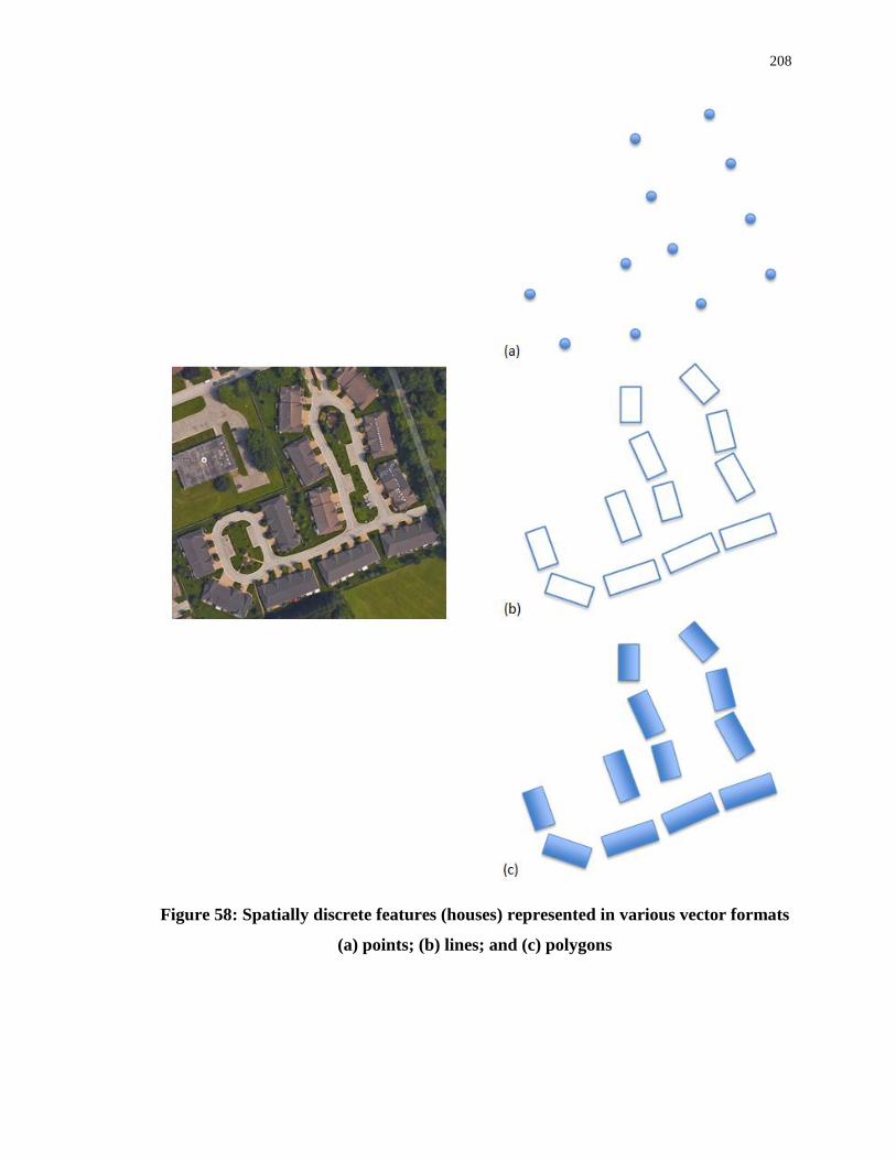
208
Figure 58: Spatially discrete features (houses) represented in various vector formats
(a) points; (b) lines; and (c) polygons

209
Spatial Reference Systems: Every spatial dataset is mapped using a reference coordinate
system. There are two types of coordinate systems: geographical coordinate systems and
projected coordinate systems.
Geographic coordinate systems (GCSs) represent the location of features on the earth’s
surface relative to the earth’s center. Projected coordinate systems (PCSs) are the location
of features defined on a 2D planar representation of the earth’s surface. PCSs are always
based on a GCS, which in turn uses an approximation of the earth’s shape as a spheroid.
Locations referenced using GCSs are defined by a latitude and longitude relative to a global
datum.
Each coordinate system may be defined by different units of measurement (feet, meters, or
degrees), shifts, and reference datum, adding to the complexity of working with multiple
GIS datasets. Any distances and measurements made between datasets with different
coordinate systems are not necessarily equal. Therefore, one of the first steps in working
with spatial data is to make datasets compatible by ensuring they are share similar spatial
reference information. To achieve this, datasets commonly require geographic datum
transformations to convert coordinates between two geographic coordinate systems.
Failure to correctly transform datasets could cause misalignments anywhere from a few
centimeters to a few hundred meters.
Mathematical transformations help translate the data from a spheroid (the approximate
shape of the Earth) to a flat 2D surface (a map). A transformation is required to go from a
GCS to PCS because reality is distorted in some way when translating 3D positions onto
2D maps. Map projections “roll out” the 3D shape of the Earth onto a 2D surface based on
a particular shape; conical, cylindrical, and planar are some of the most common shapes
used in map projections. Each projection preserves different spatial properties, therefore
reducing the distortion of the projection in different ways. Selecting the appropriate
projection is driven by the questions and analytical goals of the spatial analysis.
GCSs commonly used in Canada include: North American Datum 1927 (NAD 1927),
North American Datum 1983 (NAD 1983), and Canadian Spatial Reference System 98
(CSRS98). PCSs commonly used in Canada include: Universal Trans Mercator (UTM), 10

210
Degree Transverse Mercator (10TM), and Albers Equal Area Conic. Since the DRST relies
on spatial data collected from multiple sources, GCS and PCS transformations were
required. Ensuring that datasets are geographically compatible by having all input and
output layers mapped in the same working environment is one of the first procedures
executed by the DRST.
Vertical coordinate systems are also important to spatial analysis when considering the
representation of elevations or depths. The units of measurement in vertical coordinate
systems are always linear (feet or meters). The z-axis direction may be positive in the
upwards direction (representing positive elevation values) and negative in the downwards
direction (representing depths below the reference point). However, it is possible that some
vertical coordinate systems define the z-axis upwards direction as negative and the
downwards z-direction as positive. Thus, it is important that the vertical coordinate systems
of datasets using elevations or depth data be compatible. Since the DRST uses spatial
elevation and depths as part of the analysis, the datasets had to satisfy this criterion.
To ensure compatible coordinate systems between all of the spatial data, one of the first
things the DRST does is set these characteristics in the spatial geoprocessing environment.
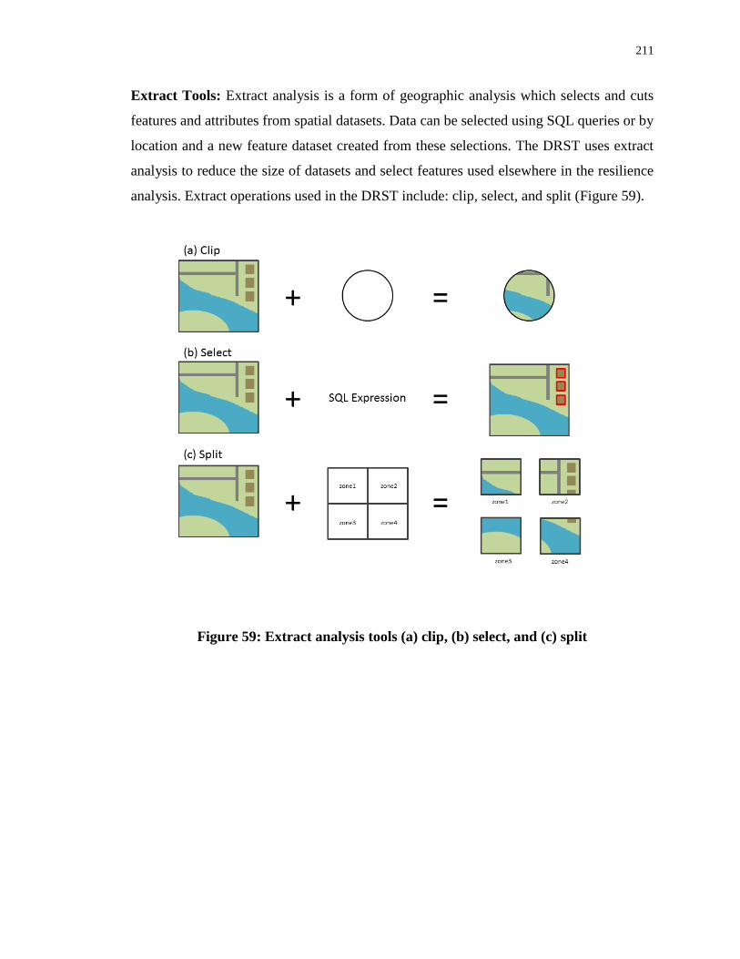
211
Extract Tools: Extract analysis is a form of geographic analysis which selects and cuts
features and attributes from spatial datasets. Data can be selected using SQL queries or by
location and a new feature dataset created from these selections. The DRST uses extract
analysis to reduce the size of datasets and select features used elsewhere in the resilience
analysis. Extract operations used in the DRST include: clip, select, and split (Figure 59).
Figure 59: Extract analysis tools (a) clip, (b) select, and (c) split
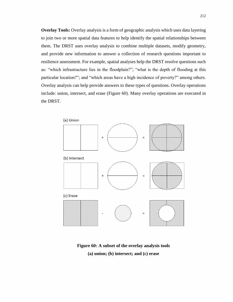
212
Overlay Tools: Overlay analysis is a form of geographic analysis which uses data layering
to join two or more spatial data features to help identify the spatial relationships between
them. The DRST uses overlay analysis to combine multiple datasets, modify geometry,
and provide new information to answer a collection of research questions important to
resilience assessment. For example, spatial analyses help the DRST resolve questions such
as: “which infrastructure lies in the floodplain?”; “what is the depth of flooding at this
particular location?”; and “which areas have a high incidence of poverty?” among others.
Overlay analysis can help provide answers to these types of questions. Overlay operations
include: union, intersect, and erase (Figure 60). Many overlay operations are executed in
the DRST.
Figure 60: A subset of the overlay analysis tools
(a) union; (b) intersect; and (c) erase

213
Proximity Tools: Proximity analysis is a form of geographic analysis which uses data
layering to identify spatial relationships between data to help the DRST resolve questions
such as: “what is near what?” Proximity analyses involve the use of buffers, distances,
directions, routes, and allocations to identify how close features are to each other; the
nearest and farthest features from a source; and the shortest distance between two or more
features. Proximity analysis tools can be divided into vector (feature) and raster-based
tools. The primary raster-based proximity analysis tool used by the DRST is called cost-
distance. Cost-distance analysis uses the relative spatial location of features to measure
distances. This tool uniquely considers that distance can be evaluated in terms of cost (such
as difficulty, dollar cost, energy expenditure, time, etc.), instead of traditional distance units
(meters, feet, etc.). The algorithm behind the tool then calculates the cumulative least cost
path to the cell(s) of interest (Figure 61).
Figure 61: Cost distance proximity analysis
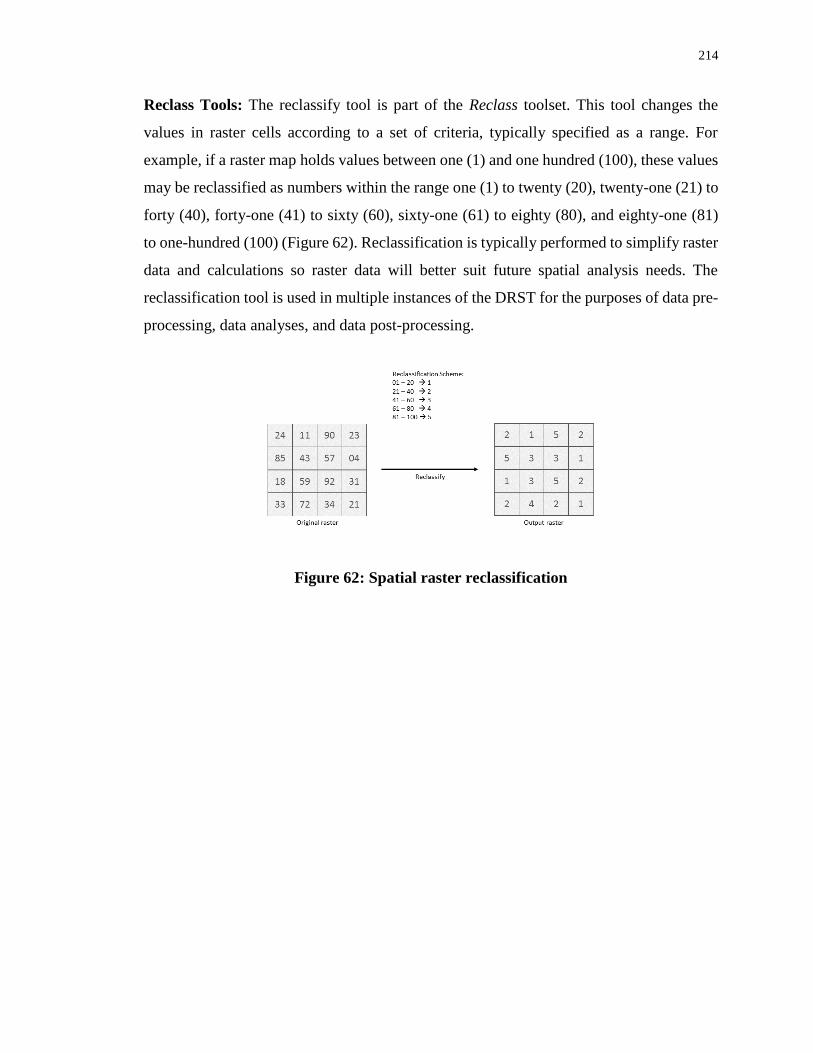
214
Reclass Tools: The reclassify tool is part of the Reclass toolset. This tool changes the
values in raster cells according to a set of criteria, typically specified as a range. For
example, if a raster map holds values between one (1) and one hundred (100), these values
may be reclassified as numbers within the range one (1) to twenty (20), twenty-one (21) to
forty (40), forty-one (41) to sixty (60), sixty-one (61) to eighty (80), and eighty-one (81)
to one-hundred (100) (Figure 62). Reclassification is typically performed to simplify raster
data and calculations so raster data will better suit future spatial analysis needs. The
reclassification tool is used in multiple instances of the DRST for the purposes of data pre-
processing, data analyses, and data post-processing.
Figure 62: Spatial raster reclassification
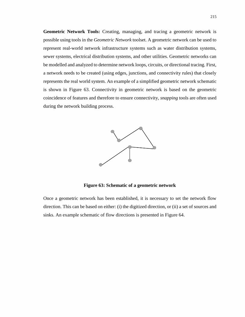
215
Geometric Network Tools: Creating, managing, and tracing a geometric network is
possible using tools in the Geometric Network toolset. A geometric network can be used to
represent real-world network infrastructure systems such as water distribution systems,
sewer systems, electrical distribution systems, and other utilities. Geometric networks can
be modelled and analyzed to determine network loops, circuits, or directional tracing. First,
a network needs to be created (using edges, junctions, and connectivity rules) that closely
represents the real world system. An example of a simplified geometric network schematic
is shown in Figure 63. Connectivity in geometric network is based on the geometric
coincidence of features and therefore to ensure connectivity, snapping tools are often used
during the network building process.
Figure 63: Schematic of a geometric network
Once a geometric network has been established, it is necessary to set the network flow
direction. This can be based on either: (i) the digitized direction, or (ii) a set of sources and
sinks. An example schematic of flow directions is presented in Figure 64.
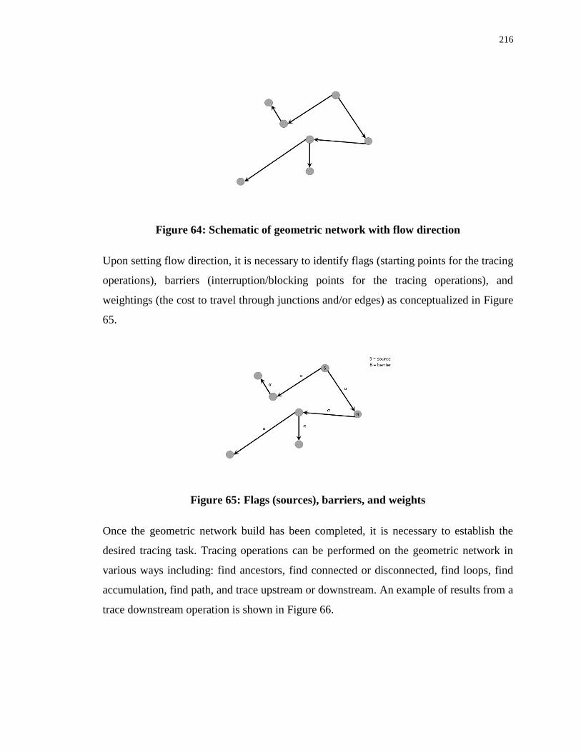
216
Figure 64: Schematic of geometric network with flow direction
Upon setting flow direction, it is necessary to identify flags (starting points for the tracing
operations), barriers (interruption/blocking points for the tracing operations), and
weightings (the cost to travel through junctions and/or edges) as conceptualized in Figure
65.
Figure 65: Flags (sources), barriers, and weights
Once the geometric network build has been completed, it is necessary to establish the
desired tracing task. Tracing operations can be performed on the geometric network in
various ways including: find ancestors, find connected or disconnected, find loops, find
accumulation, find path, and trace upstream or downstream. An example of results from a
trace downstream operation is shown in Figure 66.

217
Figure 66: Conceptual results from a trace downstream operation in a geometric
network
A geometric network was created in ArcGIS to represent power transmission network as
part of the implementation of social domain in the DRST. It uses the trace downstream
operation to identify all network features that lie downstream of a given point in the
network. The trace operation is executed at each time step to determine outages in the
transmission network during a flood event.
It should be also be noted, however, that the implementation of geometric network tracing
in ArcMap differs from the way in which is needs to be programmed in the Python
middleware program. Although geometric network tracing tools (as part of ArcPy) are
used, the way in which barriers, flags, and tracing is executed does not map directly from
the use of the tool within the ArcMap interface. To see how this tool was implemented in
a Python environment, the reader is referred to the documentation of the Python
middleware program provided in Appendix F (electronically).

218
Appendix B
VIC Hydrologic Model Equations
The following is a list of the basic mathematical equations used in the VIC hydrologic model. This model was used to simulate climate
change influenced streamflows for the Fraser River Basin. The VIC model is based on the original work of Liang et al. (1994), which
has since been updated to VIC 5 model Hamman et al. (2018) to include improvements in the flexibility and accuracy of the model, but
remains fundamentally built on the equations below. The snow accumulation and ablation models were created consider the work of
Andreadis et al. (2009). The climate change influenced hydrologic simulations were completed by Pacific Climate Impacts Consortium
(PCIC) using the VIC model.
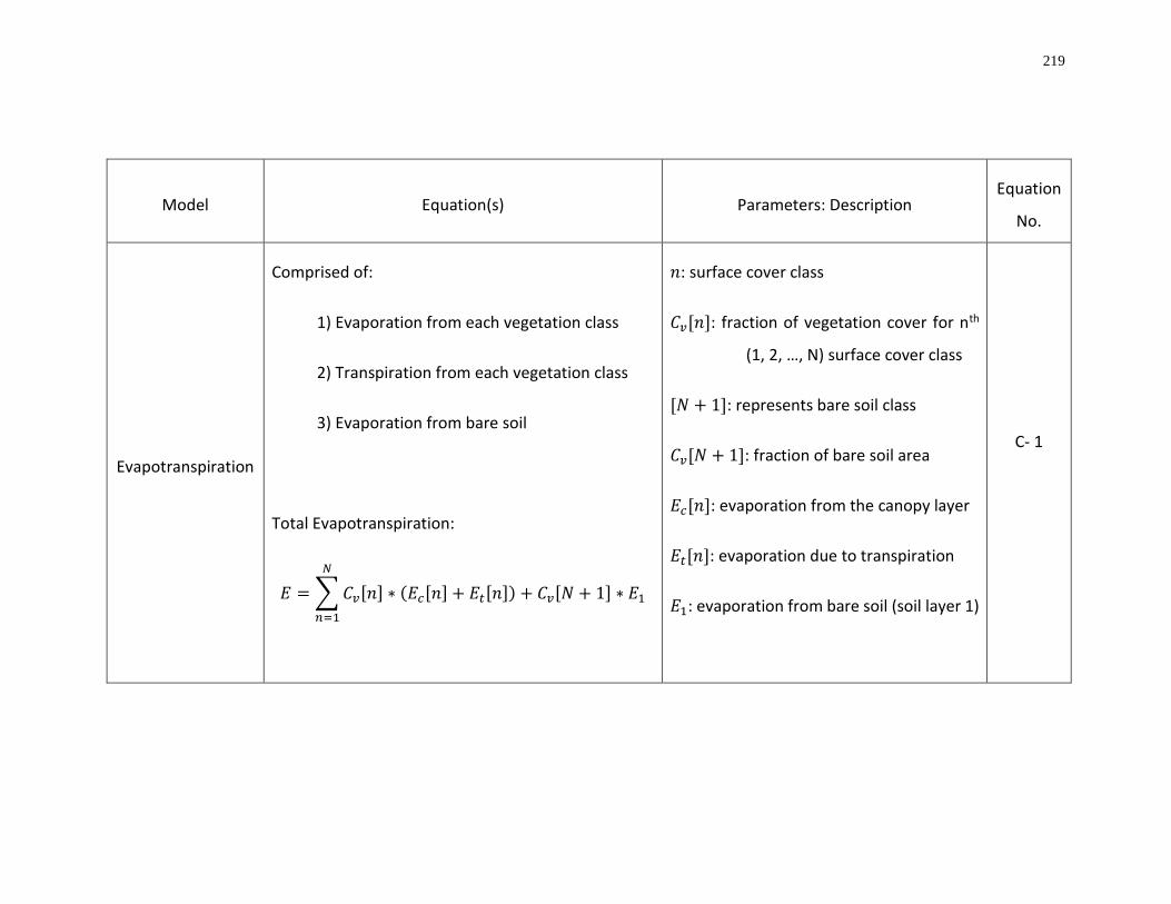
219
Model Equation(s) Parameters: Description Equation
No.
Evapotranspiration
Comprised of:
1) Evaporation from each vegetation class
2) Transpiration from each vegetation class
3) Evaporation from bare soil
Total Evapotranspiration:
𝐸 = ∑ 𝐶𝑣[𝑛] ∗ (𝐸𝑐[𝑛] + 𝐸𝑡[𝑛]) + 𝐶𝑣[𝑁 + 1] ∗ 𝐸1
𝑁
𝑛=1
𝑛: surface cover class
𝐶𝑣[𝑛]: fraction of vegetation cover for nth
(1, 2, …, N) surface cover class
[𝑁 + 1]: represents bare soil class
𝐶𝑣[𝑁 + 1]: fraction of bare soil area
𝐸𝑐[𝑛]: evaporation from the canopy layer
𝐸𝑡[𝑛]: evaporation due to transpiration
𝐸1: evaporation from bare soil (soil layer 1)
C- 1

220
Interception
(canopy layer
water balance)
𝑑𝑊𝑖[𝑛]
𝑑𝑡= 𝑃 − 𝐸𝑐[𝑛] − 𝑃𝑡[𝑛]
when
0 ≤ 𝑊𝑖[𝑛] ≤ 𝑊𝑖𝑚[𝑛]
and
𝑊𝑖𝑚[𝑛] = 𝐾𝐿 ∗ 𝐿𝐴𝐼[𝑛, 𝑚𝑜𝑛𝑡ℎ]
𝑃: precipitation rate
𝑃𝑡[𝑛]: throughfall of precipitation
𝑊𝑖[𝑛]: amount of water intercepted by the
canopy
𝑊𝑖𝑚[𝑛]: maximum amount of water
intercepted by the canopy
𝐾𝐿: constant of 0.2mm
𝐿𝐴𝐼[𝑛, 𝑚𝑜𝑛𝑡ℎ]: leaf area index for the nth
type of surface cover class for a particular
month
C- 2
Drainage
(soil layer 1 to soil
layer 2)
𝑄12[𝑛] = 𝐾𝑠 (𝑊1[𝑛] − 𝜃𝑟
𝑊1𝑐 − 𝜃𝑟
)
2𝐵𝑝
+3
𝐾𝑠: saturated soil conductivity
𝜃𝑟: residual moisture content
𝐵𝑝: pore size distribution index
C- 3
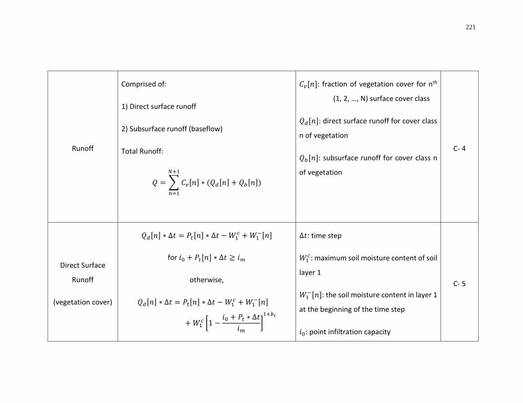
221
Runoff
Comprised of:
1) Direct surface runoff
2) Subsurface runoff (baseflow)
Total Runoff:
𝑄 = ∑ 𝐶𝑣[𝑛] ∗ (𝑄𝑑[𝑛] + 𝑄𝑏[𝑛])
𝑁+1
𝑛=1
𝐶𝑣[𝑛]: fraction of vegetation cover for nth
(1, 2, …, N) surface cover class
𝑄𝑑[𝑛]: direct surface runoff for cover class
n of vegetation
𝑄𝑏[𝑛]: subsurface runoff for cover class n
of vegetation
C- 4
Direct Surface
Runoff
(vegetation cover)
𝑄𝑑[𝑛] ∗ ∆𝑡 = 𝑃𝑡[𝑛] ∗ ∆𝑡 − 𝑊1𝑐 + 𝑊1
−[𝑛]
for 𝑖0 + 𝑃𝑡[𝑛] ∗ ∆𝑡 ≥ 𝑖𝑚
otherwise,
𝑄𝑑[𝑛] ∗ ∆𝑡 = 𝑃𝑡[𝑛] ∗ ∆𝑡 − 𝑊1𝑐 + 𝑊1
−[𝑛]
+ 𝑊1𝑐 [1 −
𝑖0 + 𝑃𝑡 ∗ ∆𝑡
𝑖𝑚]
1+𝑏𝑖
∆𝑡: time step
𝑊1𝑐: maximum soil moisture content of soil
layer 1
𝑊1−[𝑛]: the soil moisture content in layer 1
at the beginning of the time step
𝑖0: point infiltration capacity
C- 5

222
for 𝑖0 + 𝑃𝑡[𝑛] ∗ ∆𝑡 ≤ 𝑖𝑚
𝑖𝑚: maximum infiltration capacity
𝑏𝑖: infiltration shape parameter
Subsurface Runoff
(vegetation cover)
𝑄𝑏[𝑛] =𝐷𝑠𝐷𝑚
𝑊𝑠𝑊2𝑐 𝑊2
−[𝑛]
for 0 ≤ 𝑊2−[𝑛] ≤ 𝑊𝑠𝑊2
𝑐
otherwise,
𝑄𝑏[𝑛] =𝐷𝑠𝐷𝑚
𝑊𝑠𝑊2𝑐 𝑊2
−[𝑛]
+ (𝐷𝑚 −𝐷𝑠𝐷𝑚
𝑊𝑠) (
𝑊2−[𝑛] − 𝑊𝑠𝑊2
𝑐
𝑊2𝑐 − 𝑊𝑠𝑊2
𝑐 )
2
for 𝑊2−[𝑛] ≥ 𝑊𝑠𝑊2
𝑐
𝐷𝑚: maximum subsurface flow
𝐷𝑠: fraction of maximum subsurface flow
𝑊2𝑐: maximum soil moisture content of soil
layer 2
𝑊𝑠: fraction of maximum soil moisture
content of soil layer 2
𝑊2−[𝑛]: soil moisture content of soil layer 2
at the beginning of the time step
Note: 𝐷𝑠 ≤ 𝑊𝑠
C- 6
Aerodynamic Flux
Net radiation: 𝐻[𝑛]: sensible heat flux
𝜌𝑤: density of water
C- 7

223
𝑅𝑛[𝑛] = 𝐻[𝑛] + 𝜌𝑤𝐿𝑒𝐸[𝑛] + 𝐺[𝑛] + ∆𝐻𝑠[𝑛]
𝐿𝑒: latent heat of vaporization
𝜌𝑤𝐿𝑒𝐸[𝑛]: is latent heat flux
𝐺[𝑛]: ground heat flux
∆𝐻𝑠[𝑛]: change in energy storage in the
layer, per unit time, per unit area
Snow
Ground snowpack (2-layer):
𝜌𝑤𝑐𝑠
𝑑𝑊𝑡𝑠
𝑑𝑡= 𝑄𝑟 + 𝑄𝑠 + 𝑄𝑒 + 𝑄𝑝 + 𝑄𝑚
𝑐𝑠: specific heat of ice
𝜌𝑤: density of water
𝑇𝑠: temperature of the surface layer
𝑄𝑟: net radiation flux
𝑄𝑠: sensible heat flux
𝑄𝑒: latent heat flux
𝑄𝑝: energy flux advected to the snowpack
by rain or snow
C- 8
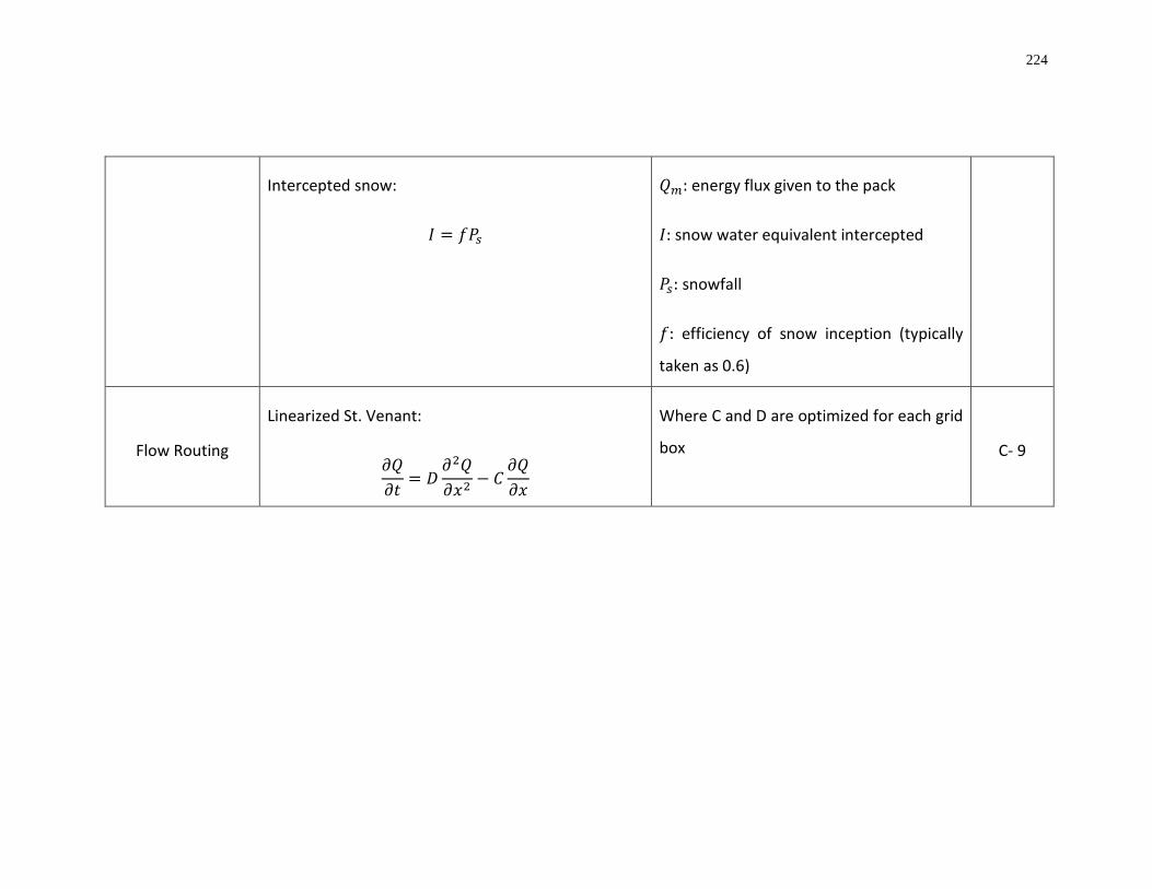
224
Intercepted snow:
𝐼 = 𝑓𝑃𝑠
𝑄𝑚: energy flux given to the pack
𝐼: snow water equivalent intercepted
𝑃𝑠: snowfall
𝑓: efficiency of snow inception (typically
taken as 0.6)
Flow Routing
Linearized St. Venant:
𝜕𝑄
𝜕𝑡= 𝐷
𝜕2𝑄
𝜕𝑥2− 𝐶
𝜕𝑄
𝜕𝑥
Where C and D are optimized for each grid
box C- 9
225
Some important assumptions and limitations of the VIC model include:
Land surface is modeled as a grid of large uniform cells
Sub-grid heterogeneity (e.g. elevation, land cover) is handled via statistical distributions
Inputs are time series of sub-daily meteorological drivers (precipitation, air temperature, wind speed, long wave radiation, short
wave radiation, atmospheric pressure, and vapor pressure) and daily land cover data (albedo, LAI, canopy cover fraction)
Land-atmosphere fluxes, and the water and energy balances at the land surface are simulated at a daily or sub-daily time step
Water can only enter a grid cell via the atmosphere
The portions of surface and subsurface runoff that reach the local channel network within a grid cell are assumed to be much
greater than the portions that cross grid cell boundaries into neighboring cells. Grid cells are simulated independently of each
other, there is no communication between grid cells and as such, non-channel flow between grid cells is ignored
Once water reaches the channel network, it is assumed to stay in the channel (it cannot flow back into the soil)
Routing of stream flow is performed separately from the land surface simulation, using a separate model

226
Appendix C
HEC-RAS Hydraulic Modelling Equations
The following is a list of the fundamental mathematical equations used as a basis for hydraulic modelling using the United States Army
Corps of Engineers (USACE) HEC-RAS software. This model was used to simulate climate change influenced inundation for the Fraser
River Basin. Hydraulic model development and simulation was performed by the author. Results were calibrated to four Water Survey
of Canada (WSC) streamflow gauges on the Fraser River network. Results were validated based on cross sections and flow data provided
by the Ministry of Forest Lands and Natural Resource Operations (MFLNRO) of British Columbia. Please note that HEC-RAS version
4.2.1 was used to perform hydraulic modelling and 1D unsteady flow simulation. Parameters were primarily derived from open data
sets available online through Land Information Ontario (LIO), Data BC, UBC’s GIS Data Catalogue, and Western University’s GIS
Library.

227
Unsteady Flow Principle
Equation Parameters Equation
No.
Continuity Equation
𝜕𝐴
𝜕𝑡+
𝜕𝑆
𝜕𝑡+
𝜕𝑄
𝜕𝑥− 𝑞𝑙 = 0
functional form:
∆𝑄 +∆𝐴𝑐
∆𝑡∆𝑥𝑐 +
∆𝐴𝑓
∆𝑡∆𝑥𝑓 +
∆𝑆
∆𝑡∆𝑥𝑓 − �̅�𝑙 = 0
𝐴: cross-sectional area 𝑡: time 𝑆: storage (from non-conveying portions of cross section) 𝑄: flow 𝑥: distance along the channel 𝑞𝑙: lateral inflow per unit distance 𝐴𝑐, 𝐴𝑓: cross sectional area of the channel
and floodplain, respectively 𝑥𝑐, 𝑥𝑓: length of the channel and floodplain,
respectively, between two cross sections �̅�𝑙: average lateral inflow
D- 1
Momentum Equation
𝜕𝑄
𝜕𝑡+
𝜕(𝑉𝑄)
𝜕𝑥+ 𝑔𝐴 (
𝜕𝑧
𝜕𝑥+ 𝑆𝑓 + 𝑆ℎ) = 0
functional form:
∆(𝑄𝑐∆𝑥𝑐 + 𝑄𝑓∆𝑥𝑓)
∆𝑡∆𝑥𝑒+
∆(𝛽𝑉𝑄)
∆𝑥𝑒
+ 𝑔�̅� (∆𝑧
∆𝑥𝑒+ 𝑆�̅� + 𝑆ℎ̅) = 0
𝑔: acceleration due to gravity 𝑆𝑓 , 𝑆ℎ: friction slope and local slope,
respectively 𝑉: velocity 𝑄𝑐, 𝑄𝑓: flow in the channel and floodplain,
respectively Δ𝑥𝑒: equivalent flow path 𝛽: velocity distribution factor 𝑧: water surface elevation
D- 2
Momentum Equation
(at a junction)
Functional form: 𝜉: fraction of momentum entering the receiving stream 𝑄𝑙: lateral inflow 𝑉𝑙: average velocity of lateral inflow
D- 3

228
∆(𝑄𝑐∆𝑥𝑐 + 𝑄𝑓∆𝑥𝑓)
∆𝑡∆𝑥𝑒+
∆(𝛽𝑉𝑄)
∆𝑥𝑒
+ 𝑔�̅� (∆𝑧
∆𝑥𝑒+ 𝑆�̅� + 𝑆ℎ̅) = 𝜉
𝑄𝑙𝑉𝑙
∆𝑥𝑒
Flow Distribution Factor
(ratio of conveyance)
𝜙 =𝑄𝑐
𝑄𝑐 + 𝑄𝑓
Functional form (assuming 𝑆𝑓 is the same for channel and
floodplain):
𝜙𝑗 =𝐾𝑐
𝐾𝑐 + 𝐾𝑓
𝐾𝑐: conveyance in the channel 𝐾𝑓: conveyance in the floodplain
* under the assumption that friction slope is the same for the channel and the floodplain
D- 4
*Additional equations and finite difference approximations for the terms in the momentum and energy equations used in the solution of
1D unsteady flow models can be found in USACE (2010). Some important assumptions and limitations of the 1D unsteady flow HEC-
RAS models include:
Water surface is horizontal at any cross section perpendicular to flow; in other words, the water surface elevation is the same
for the channel and floodplain at any given cross section
At a junction, the water surface computed at the downstream side is used for cross sections just upstream; for steeper rivers
where this is not really a good assumption, an energy balance can be performed to compute upstream water surface elevations
When solving momentum balance equation at a junction, water surface elevations at the cross sections on each tributary just
upstream of the junction are assumed to be equal to each other (as an approximation)
229
Appendix D
GAMS Programming and Documentation
The following Appendix is included to provide additional details and materials to support
the thesis text. This Appendix first describes the functionality of the economic domain of
the DRST (GAMS model) and then provides the GAMS code used as part of the DRST.
The code was developed by Aaron Gertz as part of his PhD thesis On the Economics of
Climate Change and its Effects (2015) and additional details pertaining to the development
of the program can be found in the paper:
Gertz, Aaron B. and James B. Davies. A CGE Framework for Modelling the Economics of
Flooding and Recovery in a Major Urban Area, Economic Policy Research Institute. EPRI
Working Papers, 2015-2. London, ON: Department of Economics, University of Western.
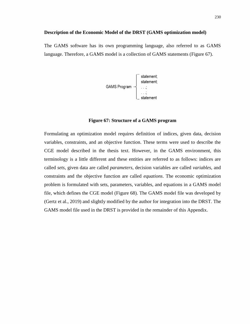
230
Description of the Economic Model of the DRST (GAMS optimization model)
The GAMS software has its own programming language, also referred to as GAMS
language. Therefore, a GAMS model is a collection of GAMS statements (Figure 67).
Figure 67: Structure of a GAMS program
Formulating an optimization model requires definition of indices, given data, decision
variables, constraints, and an objective function. These terms were used to describe the
CGE model described in the thesis text. However, in the GAMS environment, this
terminology is a little different and these entities are referred to as follows: indices are
called sets, given data are called parameters, decision variables are called variables, and
constraints and the objective function are called equations. The economic optimization
problem is formulated with sets, parameters, variables, and equations in a GAMS model
file, which defines the CGE model (Figure 68). The GAMS model file was developed by
(Gertz et al., 2019) and slightly modified by the author for integration into the DRST. The
GAMS model file used in the DRST is provided in the remainder of this Appendix.

231
Figure 68: Organization of GAMS program
When a well-defined operational GAMS model file is sent to the GAMS program, the
optimization model is formulated and solved. The GAMS program uses mathematical
optimization techniques to solve the objective functions (equations) subject to constraints
(also equations). The program then outputs results in the form of text files which contain
optimization solutions and variable values. The three allowable forms of data into a GAMS
model include: lists, tables, and direct assignments. The DRST makes use of all three
fundamentally different formats, however the primary data input format is tables, including
matrices.
GAMS software is file-based and offers open architecture in which the user can create or
edit files using their preferred word processor. Since GAMS files require no special editor,
the input and output files can be easily integrated with other programs. This is useful for
the implementation of the DRST, since some of the input files become modified in the
event of a flood. The DRST invokes GAMS using a Python script. The object-oriented
GAMS Python API provides access to GAMS from within a Python program. This is used
to bridge between the economics modelling, SD simulations, and GIS analysis components
of the DRST. The Python script developed as part of this research provides the functionality
and automation for all three modelling, simulation, and optimization tools from the
convenience of a single program.

232
$TITLE Model Van: dynamic model of Vancouver economy.
$ONTEXT
$OFFTEXT
TABLE BENCH(*,*) Benchmark financial flows (e.g. an input-output table)
$ondelim
$include VAN_20x20_all_adj.csv
$offdelim
TABLE E_CAP(*,*) Exposed capital to flooding by industry
$ondelim
$include exposed_capital.csv
$offdelim
SET T Time periods /1*220/,
TFIRST(T),
TLAST(T),
TAID(T),
I Produced goods /BS11, BS21, BS22, BS23, BS31, BS41, BS44,
BS48, BS51, BS52, BS54, BS56, BS61, BS62, BS71, BS72, BS81,
GS61, GS62, GS91/,
F Factors of production /L, K/,
TX Taxes /ST, CIT, LIT, KIT/
FD Final demand sectors /W, G, INVP, INVG, E, M/;
ALIAS (I,J), (F,FF);

233
TFIRST(T) = YES$(ORD(T) EQ 1);
TLAST(T) = YES$(ORD(T) EQ CARD(T));
SCALAR TS TIMESTEPS IN 1 YEAR /4/
DR DAMAGE RATE OF EXPOSED CAPITAL /0.25/
LRK TEMP LOSS RATE OF CAPITAL /0/
LRL TEMP LOSS RATE OF LABOUR /0/
YA YEARS OVER WHICH AID IS SPREAD /2/
AIDP FRACTION OF DAMAGE COVERED BY AID /0.75/
DELTA DEPRECIATION /0.05/
* DELTA DEPRECIATION /0.10/
R INTEREST RATE /0.0762713752792/
* R INTEREST RATE /0.1303876789703/
*for g = 0.05
* R INTEREST RATE /0.1164652147643/
*for delta = 0.1
G GROWTH RATE /0.02/
* G GROWTH RATE /0.05/
RK0 INITIAL RETURN TO CAPITAL;
TAID(T) = YES$(ORD(T) LE YA*TS);
PARAMETERS
QREF(T) Quantities,
PREF(T) Prices,
Q0(I) Benchmark gross domestic output,
ID0(J,I) Benchmark Intermediate demands,
FS0(F,I) Benchmark factor supplies,
VL(I) Benchmark labour earnings,
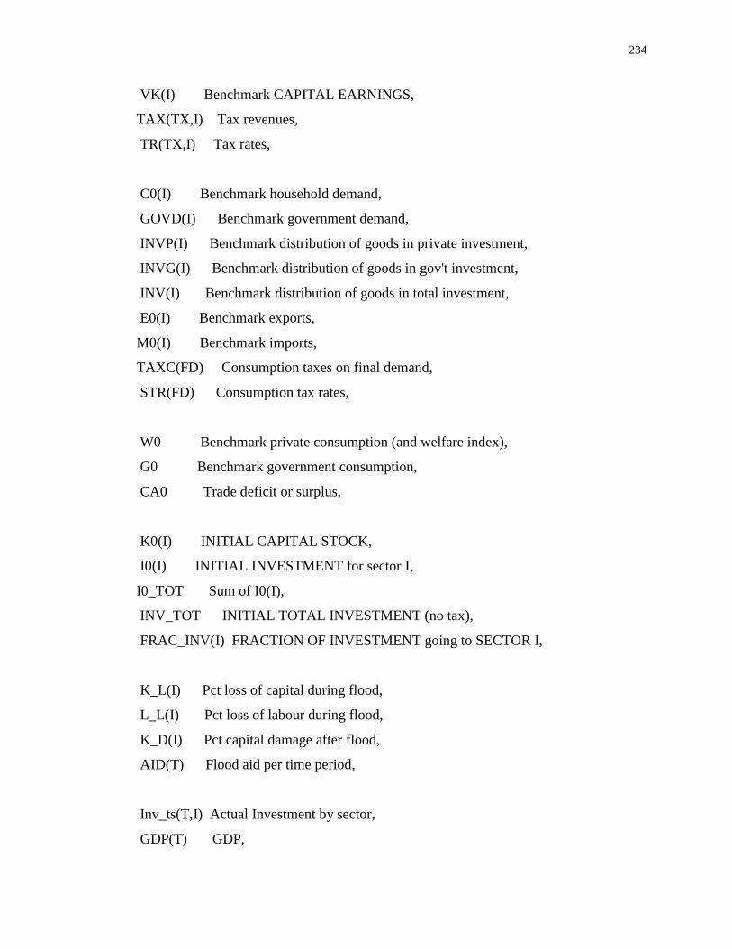
234
VK(I) Benchmark CAPITAL EARNINGS,
TAX(TX,I) Tax revenues,
TR(TX,I) Tax rates,
C0(I) Benchmark household demand,
GOVD(I) Benchmark government demand,
INVP(I) Benchmark distribution of goods in private investment,
INVG(I) Benchmark distribution of goods in gov't investment,
INV(I) Benchmark distribution of goods in total investment,
E0(I) Benchmark exports,
M0(I) Benchmark imports,
TAXC(FD) Consumption taxes on final demand,
STR(FD) Consumption tax rates,
W0 Benchmark private consumption (and welfare index),
G0 Benchmark government consumption,
CA0 Trade deficit or surplus,
K0(I) INITIAL CAPITAL STOCK,
I0(I) INITIAL INVESTMENT for sector I,
I0_TOT Sum of I0(I),
INV_TOT INITIAL TOTAL INVESTMENT (no tax),
FRAC_INV(I) FRACTION OF INVESTMENT going to SECTOR I,
K_L(I) Pct loss of capital during flood,
L_L(I) Pct loss of labour during flood,
K_D(I) Pct capital damage after flood,
AID(T) Flood aid per time period,
Inv_ts(T,I) Actual Investment by sector,
GDP(T) GDP,

235
GR(T) GDP growth rate,
LAB(T,I) Labour,
ESUB(I) Armington elasticity of substitution;
R = R/TS;
G = G/TS;
DELTA = DELTA/TS;
QREF(T) = (1 + G) ** (ORD(T) - 1);
PREF(T) = (1/(1 + R)) ** (ORD(T) - 1);
*Input-output
Q0(I) = BENCH(I,I);
ID0(J,I) = MAX(0, -BENCH(J,I));
VL(I) = -BENCH("L",I);
VK(I) = -BENCH("K",I);
TAX(TX,I) = -BENCH(TX,I);
*Final Demand
C0(I) = -BENCH(I,"W");
GOVD(I) = -BENCH(I,"G");
INVP(I) = -BENCH(I,"INVP");
INVG(I) = -BENCH(I,"INVG");
INV(I) = INVP(I) + INVG(I);
E0(I) = -BENCH(I,"E");
M0(I) = BENCH(I,"M");
TAXC(FD) = -BENCH("ST",FD);
INV_TOT = SUM(I, INV(I));

236
FRAC_INV(I) = INV(I)/INV_TOT;
W0 = BENCH("W","W");
G0 = BENCH("W","G");
CA0 = BENCH("FX","CONS");
*Input taxes
TR("ST",I) = TAX("ST",I)/sum(J,ID0(J,I));
TR("CIT",I) = TAX("CIT",I)/VK(I);
TR("LIT",I) = TAX("LIT",I)/VL(I);
TR("KIT",I) = TAX("KIT",I)/VK(I);
STR("INVP") = (TAXC("INVP")+TAXC("INVG"))/INV_TOT;
*Output taxes
STR("W") = TAXC("W")/W0;
STR("G") = TAXC("G")/G0;
STR("E") = TAXC("E")/(sum(I,E0(I))+TAXC("E"));
STR("M") = TAXC("M")/(sum(I,M0(I))+TAXC("M"));
*Capital, investment and rate of return calculations
RK0 = (DELTA + R)*(1+STR("INVP"));
K0(I) = VK(I)/RK0;
I0(I) = (DELTA + G) * K0(I);
I0_TOT = sum(I,I0(I));
*Damages and losses plus aid
FS0("L",I) = VL(I);
FS0("K",I) = K0(I);
K_L(I) = LRK*E_CAP(I,"KLOSS");

237
L_L(I) = LRL*E_CAP(I,"LLOSS");
K_D(I) = DR*E_CAP(I,"KDAM");
AID(T)$TAID(T) = AIDP*SUM(I,K_D(I)*K0(I))/(YA*TS);
ESUB(I) = 3;
$ONTEXT
$MODEL:Van
$SECTORS:
X(T,I) ! Activity level for sector I
W(T) ! Activity level for sector W (welfare index)
GC(T) ! Activity level for sector GC (government consumption bundle)
KN(T,I) ! Investment sector
K(T,I) ! Capital accumulation
M(T,I) ! Imports
E(T,I) ! Exports
ARM(T,I) ! Armington goods
$COMMODITIES:
P(T,I) ! Price index for commodities
PL(T,I) ! Price index for primary factor L
PK(T,I) ! Price index for primary factor K
PW(T) ! Price index for welfare (expenditure function)
PG(T) ! Price index for government bundle
RK(T,I) ! Rental rate for capital
PKT(I) ! Post-terminal capital constraint
FR(T) ! Real exchange rate
PF(T,I) ! Price index for foreign commodity

238
PA(T,I) ! Price index for Armington good
$CONSUMERS:
CONS ! Income level for consumer household
GOVT ! Income level for government
$AUXILIARY:
TK(I) ! Terminal Capital Stock
$PROD:X(T,I) s:0 va:0.4
O:P(T,I) Q:Q0(I)
I:PA(T,J) Q:ID0(J,I) P:(1+TR("ST",I)) A:GOVT T:TR("ST",I)
I:PL(T,I) Q:VL(I) P:(1+TR("LIT",I)) A:GOVT T:TR("LIT",I) va:
I:RK(T,I) Q:K0(I) P:(RK0*(1+TR("KIT",I)+TR("CIT",I))) A:GOVT
T:TR("KIT",I) A:GOVT T:TR("CIT",I) va:
$PROD:K(T,I)
O:PK(T+1,I) Q:((1-DELTA)*K0(I))
O:PKT(I)$TLAST(T) Q:((1-DELTA)*K0(I))
O:RK(T,I) Q:K0(I)
I:PK(T,I) Q:K0(I)
$PROD:KN(T,I)
O:PK(T+1, I) Q:I0(I)
O:PKT(I)$TLAST(T) Q:I0(I)
I:PA(T,J) Q:(FRAC_INV(J)*I0(I)) P:(1+STR("INVP")) A:GOVT
T:STR("INVP")
$PROD:M(T,I)
O:PF(T,I) Q:((1+STR("M"))*M0(I)) A:GOVT T:STR("M")
I:FR(T) Q:M0(I)

239
$PROD:E(T,I)
O:FR(T) Q:((1+STR("E"))*E0(I)) A:GOVT T:STR("E")
I:PA(T,I) Q:E0(I)
$PROD:ARM(T,I) s:ESUB(I)
O:PA(T,I) Q:(Q0(I)+M0(I))
I:P(T,I) Q:Q0(I)
I:PF(T,I) Q:M0(I)
$PROD:W(T) s:1
O:PW(T) Q:W0 A:GOVT T:STR("W")
I:PA(T,I) Q:C0(I)
$PROD:GC(T) s:0
O:PG(T) Q:G0 A:GOVT T:STR("G")
I:PA(T,I) Q:GOVD(I)
$DEMAND:CONS s:1
D:PW(T) Q:(sum(I,C0(I))*QREF(T)) P:PREF(T)
E:PL(T,I) Q:(FS0("L",I)*QREF(T))
E:PK(TFIRST,I) Q:FS0("K",I)
E:FR(T) Q:(CA0*QREF(T))
E:FR(T) Q:AID(T)
E:PKT(I) Q:(-1) R:TK(I)
$DEMAND:GOVT s:1
D:PG(T) Q:(sum(I,GOVD(I))*QREF(T)) P:PREF(T)
$CONSTRAINT:TK(I)
SUM(T$TLAST(T), KN(T,I)/KN(T-1,I) - X(T,I)/X(T-1,I)) =G= 0;
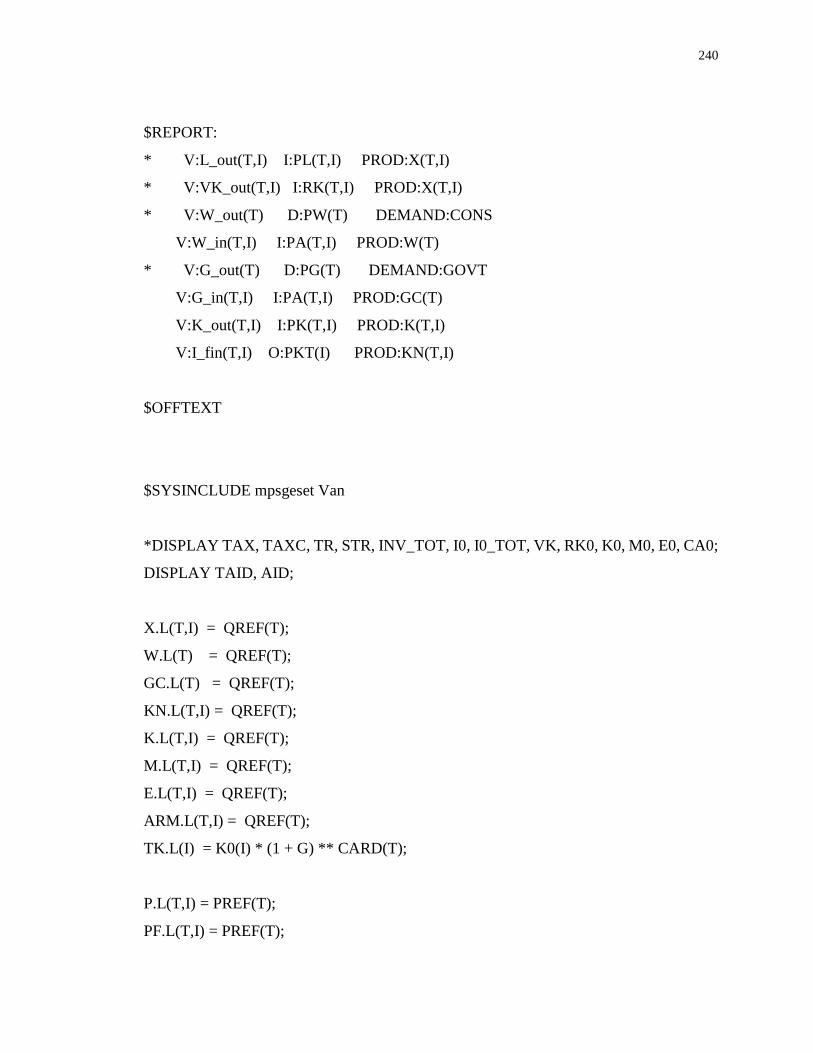
240
$REPORT:
* V:L_out(T,I) I:PL(T,I) PROD:X(T,I)
* V:VK_out(T,I) I:RK(T,I) PROD:X(T,I)
* V:W_out(T) D:PW(T) DEMAND:CONS
V:W_in(T,I) I:PA(T,I) PROD:W(T)
* V:G_out(T) D:PG(T) DEMAND:GOVT
V:G_in(T,I) I:PA(T,I) PROD:GC(T)
V:K_out(T,I) I:PK(T,I) PROD:K(T,I)
V:I_fin(T,I) O:PKT(I) PROD:KN(T,I)
$OFFTEXT
$SYSINCLUDE mpsgeset Van
*DISPLAY TAX, TAXC, TR, STR, INV_TOT, I0, I0_TOT, VK, RK0, K0, M0, E0, CA0;
DISPLAY TAID, AID;
X.L(T,I) = QREF(T);
W.L(T) = QREF(T);
GC.L(T) = QREF(T);
KN.L(T,I) = QREF(T);
K.L(T,I) = QREF(T);
M.L(T,I) = QREF(T);
E.L(T,I) = QREF(T);
ARM.L(T,I) = QREF(T);
TK.L(I) = K0(I) * (1 + G) ** CARD(T);
P.L(T,I) = PREF(T);
PF.L(T,I) = PREF(T);
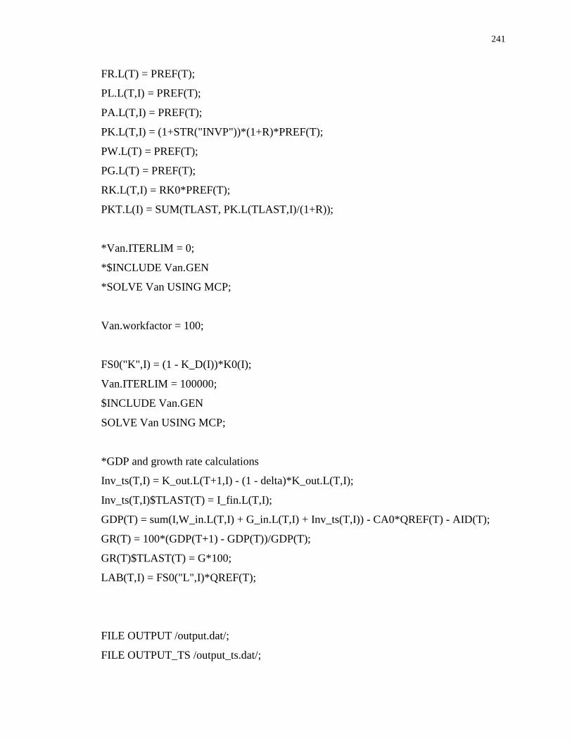
241
FR.L(T) = PREF(T);
PL.L(T,I) = PREF(T);
PA.L(T,I) = PREF(T);
PK.L(T,I) = (1+STR("INVP"))*(1+R)*PREF(T);
PW.L(T) = PREF(T);
PG.L(T) = PREF(T);
RK.L(T,I) = RK0*PREF(T);
PKT.L(I) = SUM(TLAST, PK.L(TLAST,I)/(1+R));
*Van.ITERLIM = 0;
*$INCLUDE Van.GEN
*SOLVE Van USING MCP;
Van.workfactor = 100;
FS0("K",I) = (1 - K_D(I))*K0(I);
Van.ITERLIM = 100000;
$INCLUDE Van.GEN
SOLVE Van USING MCP;
*GDP and growth rate calculations
Inv_ts(T,I) = K_out.L(T+1,I) - (1 - delta)*K_out.L(T,I);
Inv_ts(T,I)$TLAST(T) = I_fin.L(T,I);
GDP(T) = sum(I,W_in.L(T,I) + G_in.L(T,I) + Inv_ts(T,I)) - CA0*QREF(T) - AID(T);
GR(T) = 100*(GDP(T+1) - GDP(T))/GDP(T);
GR(T)$TLAST(T) = G*100;
LAB(T,I) = FS0("L",I)*QREF(T);
FILE OUTPUT /output.dat/;
FILE OUTPUT_TS /output_ts.dat/;

242
*FILE OUTPUT_D_AID /output_ts_aid.dat/;
output.nd = 5;
output_ts.nd = 5;
PUT OUTPUT;
PUT @2, 'T', @8, 'I', @19, 'X', @31, 'P', @43, 'E', @55, 'M', @66, 'PF', @79, 'K', @90,
'RK', @103, 'L', @114, 'PL'/;
LOOP(T,
LOOP(I,
PUT @1, T.TL, @5, I.TL, @9, X.L(T,I), @20, P.L(T,I), @32, E.L(T,I), @44, M.L(T,I),
@56, PF.L(T,I), @68, K_out.L(T,I), @80, RK.L(T,I), @92, LAB(T,I), @104,
PL.L(T,I)/));
PUT OUTPUT_TS;
PUT @2, 'T', @13, 'GDP', @27, 'W', @38, 'PW', @51, 'G', @62, 'PG', @74, 'FX', @86,
'GR'/;
LOOP(T,
PUT @1, T.TL, @4, GDP(T), @16, W.L(T), @28, PW.L(T), @40, GC.L(T), @52,
PG.L(T), @64, FR.L(T), @76, GR(T)/);
*PUT OUTPUT_D_AID;
*PUT @2, 'T', @13, 'AID'/;
*LOOP(T,
*PUT @1, T.TL, @4, AID(T)/);

243
Appendix E
Data to Support the Application of Resilience Quantification Framework for Metro
Vancouver, British Columbia, Canada
The following Appendix is included to support the application of the resilience quantification framework to Metro Vancouver, BC.
The following is a list of the data used in the creation of the model, the source of the data, and a brief description of the dataset.
Supporting data files are included as part of the electronic submission, note that some of these files, while spatial in nature, are saved
as matrices and require post-processing to visualize the data. Note also that there is overlap between some of the data files. This is
because multiple variables and variable attributes may be contained in a single .shp or database file.

244
Table 9: Description of Model Input Data
Model
Domain Data Name Data Type
Data
Source(s) Data Description
File Location in
Electronic
Submission
& Note(s)
All
Base imagery Aerial
Photo DataBC
Detailed aerial imagery for the Metro
Vancouver area Input geodatabase
Digital Elevation
Model (DEM) Spatial DataBC High resolution digital elevations data Hydraulics Folder
Dissemination Areas Spatial
Statistics
Canada
Census Data
Dissemination Area boundaries for Metro
Vancouver Input geodatabase
Municipal boundaries Spatial GeoBase Boundaries for each of the 21
municipalities in Metro Vancouver Input geodatabase
Economic
Input-Output table Numerical Gertz (2015) Input-output table that is used by GAMS
in economic modelling Economics folder
Roll number
Numerical
and
Spatial
BCA
The identifier (ID) for each piece of
infrastructure, used to link spatial and
numerical data
Input geodatabase
Buildings by industry Numerical BCA An industry categorization of each
building, by address Input geodatabase
Engineering
Building value Numerical BCA The reconstruction value of each
building, by address
Input geodatabase
* Note, real values
not provided due
to confidentiality
Building type Numerical BCA The building type (ex. Split-level, two-
story, …), by address Input geodatabase
Stage-Damage curves Numerical FEMA
(2015)
Depth-damage curves (depth v. %
damage) for each type of structure. Slight
Curves built
directly into
Python program.
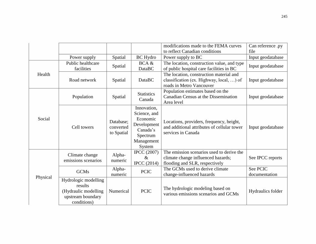
245
modifications made to the FEMA curves
to reflect Canadian conditions
Can reference .py
file
Power supply Spatial BC Hydro Power supply to BC Input geodatabase
Health
Public healthcare
facilities Spatial
BCA &
DataBC
The location, construction value, and type
of public hospital care facilities in BC Input geodatabase
Road network Spatial DataBC
The location, construction material and
classification (ex. Highway, local, …) of
roads in Metro Vancouver
Input geodatabase
Social
Population Spatial Statistics
Canada
Population estimates based on the
Canadian Census at the Dissemination
Area level
Input geodatabase
Cell towers
Database;
converted
to Spatial
Innovation,
Science, and
Economic
Development
Canada’s
Spectrum
Management
System
Locations, providers, frequency, height,
and additional attributes of cellular tower
services in Canada
Input geodatabase
Physical
Climate change
emissions scenarios
Alpha-
numeric
IPCC (2007)
&
IPCC (2014)
The emission scenarios used to derive the
climate change influenced hazards;
flooding and SLR, respectively
See IPCC reports
GCMs Alpha-
numeric PCIC
The GCMs used to derive climate
change-influenced hazards
See PCIC
documentation
Hydrologic modelling
results
(Hydraulic modelling
upstream boundary
conditions)
Numerical PCIC The hydrologic modeling based on
various emissions scenarios and GCMs Hydraulics folder

246
Hydraulic modeling
downstream boundary
conditions
Numerical MFLNRO &
Agam (2014)
The SLR boundary conditions under
various climate change scenarios Hydraulics folder
Hydraulic modeling
parameters Numerical MFLNRO Manning’s roughness coefficients Hydraulics folder
Hydraulic modeling
river geometry Spatial
DataBC /
digitization
by A. Peck
River channel, tributaries, banks, flow
direction, slopes, etc. On-screen
digitization by A. Peck using DEMs and
aerial photos
Input geodatabase
Hydraulic modeling
calibration
streamflows
Numerical
Water
Survey of
Canada
(WSC)
Four streamflow / level gauges on the
Fraser River for model calibration Hydraulics folder
Hydraulic modeling
validation cross-
sections
Numerical MFLNRO A few cross sections along the Fraser
River for model validation Hydraulics folder
247
Appendix F
Disaster Resilience Simulation Tool (DRST)
and Python Code
The following Appendix is included to provide additional details and materials to support
the dissertation text. In this Appendix, the Python code for the DRST is provided. The code
includes Vensim functions, ArcGIS functions, and GAMS functions. The code was written
from scratch using online supporting documentation provided by ESRI and Ventana
Systems. The majority of the code was written within the Spyder Python Development
Environment. It should be noted that for the Python script to run, compatible versions of
all three software must be installed on a single computer running Windows. The specific
software versions used in developing the DRST are as follows:
Windows 7 Professional SP1
Vensim DSS v. 5.10e
ArcGIS ArcMap 10.1
GAMS 24.2.3
The reader is referred to the associated files on USB / electronic submission for the .py
scripts, input files, and DRST tool with a graphical user interface. Supporting details on
the use of the DRST can be found in Appendix H.
Note: For confidentiality purposes, the building assessment values were modified for this
electronic submission. Therefore, to reproduce the results as presented in this dissertation,
would require the user to obtain MPAC data and repopulate the assessment value data
column in the associated GIS buildings file. As a placeholder, the buildings file included
as part of this submission has had the assessment value for all buildings set to a constant
value. The DRST still executes properly with this placeholder data, but will therefore not
replicate exactly the results as presented
248
Appendix G
Fraser River Hydraulic Modelling Assumptions and
Limitations
The following Appendix is included to provide additional details and materials to support
the thesis text. This Appendix provides important assumptions, limitations, and
recommendations for the hydraulic model of the Fraser River and its tributaries.
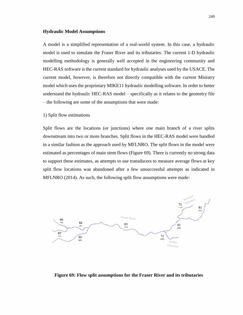
249
Hydraulic Model Assumptions
A model is a simplified representation of a real-world system. In this case, a hydraulic
model is used to simulate the Fraser River and its tributaries. The current 1-D hydraulic
modelling methodology is generally well accepted in the engineering community and
HEC-RAS software is the current standard for hydraulic analyses used by the USACE. The
current model, however, is therefore not directly compatible with the current Ministry
model which uses the proprietary MIKE11 hydraulic modelling software. In order to better
understand the hydraulic HEC-RAS model – specifically as it relates to the geometry file
– the following are some of the assumptions that were made:
1) Split flow estimations
Split flows are the locations (or junctions) where one main branch of a river splits
downstream into two or more branches. Split flows in the HEC-RAS model were handled
in a similar fashion as the approach used by MFLNRO. The split flows in the model were
estimated as percentages of main stem flows (Figure 69). There is currently no strong data
to support these estimates, as attempts to use transducers to measure average flows at key
split flow locations was abandoned after a few unsuccessful attempts as indicated in
MFLNRO (2014). As such, the following split flow assumptions were made:
Figure 69: Flow split assumptions for the Fraser River and its tributaries

250
2) Not all sources of flooding were considered
Hydraulic HEC-RAS model considers the downstream boundary conditions as tide level
plus climate change influences via sea level rise. Upstream conditions were driven by
climate change-influenced streamflow data provided by PCIC. However, there was no
considerations given to storm surge or tsunami caused inundations. At the time of writing,
design criteria and parameters for tsunami mapping in BC were not yet developed and were
not included in the hydraulic analysis.
Hydraulic Model Limitations
Some of the limitations in the hydraulic modelling include:
1) Inherent limitations of 1-D modelling
HEC-RAS is 1-D modelling software: but in some areas of the modeled region the flow
patterns are strongly 2- and 3- dimensional (MFLNRO, 2014); the lower gravel reach has
highly complex flows which may not be able to be accurately simulated by a 1-D flow
model (MFLNRO, 2014). The Ministry has made some modifications to their model to try
and address this limitation, but the complexity, data requirements, and time commitments
were too significant to address this limitation in the HEC-RAS model used for this research
and was considered out of the scope of this dissertation.
2) Exclusion of over-water infrastructure
Bridges and other over-water infrastructure were excluded from hydraulic modelling due
to time constraints and lack of detailed data. This is a very significant limitation, as some
of this infrastructure is extremely significant to emergency preparedness, response and
recovery activities. For example, the Jacob Haldi Bridge spans the Bedford Channel of the
Fraser River, connecting Fort Langley and McMillan Island. This island is home to the
Kwantlen First Nations people and the bridge is the only mainland access road to the entire
island (Figure 70). By not considering this over-water infrastructure, the potential back-
water effects the bridge may cause will be neglected in addition to potential inundation
effects on this bridge.
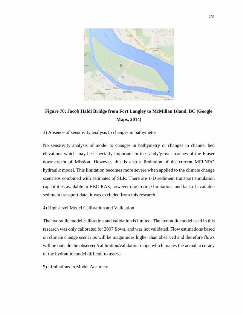
251
Figure 70: Jacob Haldi Bridge from Fort Langley to McMillan Island, BC (Google
Maps, 2014)
3) Absence of sensitivity analysis to changes in bathymetry
No sensitivity analysis of model to changes in bathymetry or changes in channel bed
elevations which may be especially important in the sandy/gravel reaches of the Fraser
downstream of Mission. However, this is also a limitation of the current MFLNRO
hydraulic model. This limitation becomes more severe when applied to the climate change
scenarios combined with estimates of SLR. There are 1-D sediment transport simulation
capabilities available in HEC-RAS, however due to time limitations and lack of available
sediment transport data, it was excluded from this research.
4) High-level Model Calibration and Validation
The hydraulic model calibration and validation is limited. The hydraulic model used in this
research was only calibrated for 2007 flows, and was not validated. Flow estimations based
on climate change scenarios will be magnitudes higher than observed and therefore flows
will be outside the observed/calibration/validation range which makes the actual accuracy
of the hydraulic model difficult to assess.
5) Limitations in Model Accuracy

252
The hydraulic model is based on many assumptions and estimations of data, and therefore
should not be used for any other purposes than for simulations and analysis using the
DRST. Given these limitations, it is important to acknowledge that there will be significant
differences between the HEC-RAS model simulated values and recorded observations at
river gauge stations.
Despite the aforementioned assumptions and limitations, it should be noted that the
inundation maps generated in this hydraulic analysis should be sufficient for making
relative comparisons of climate change impacts for the region of Metro Vancouver. The
maps generated from hydraulic analysis include estimates of future precipitation and runoff
events and incorporate regional SLR projections which is used as input into the proposed
DRST for the purposes of assessing the impacts of climate change on Metro Vancouver.
Since all scenarios are run using the same river geometry and characteristics, in relative
terms they should be adequate for relative comparisons between all of the DRST simulation
scenarios.
Hydraulic Modelling Recommendations
The following is a list of recommendations for anyone interested creating their own
hydraulic model and performing hydraulic simulation to generate inundation maps.
Although some of the recommendations are specific to modelling the Fraser River and its
tributaries, many of them could be generalized and extended in pursuit of any hydraulic
modelling effort in a large basin characterized by complex over-bank urban areas.
1) If the Ministry ever releases their MIKE11 model for open use then the proposed HEC-
RAS model should be abandoned and the Ministry’s MIKE11 model should be adopted.
The Ministry’s model will be more detailed and more accurate.
2) 1-D modelling is not sufficient for modelling complex urban environments such as the
Metro Vancouver delta region. Therefore, future studies should consider 2-D modelling
and simulation to more accurately project river flows.
3) Continued monitoring and station measurements would continue to help verify model
projections.

253
4) For any future proposed over-water infrastructure or land use changes which may
significantly modify roughness values of the right overbank, left overbank, or channel, the
hydraulic model should be updated to accommodate for these new channel geometries and
the simulations should be run again to determine if there are significant changes in flow
patterns (and corresponding floodplains).
5) Similarly, if the Ministry releases any more detailed information on their hydraulic
analysis, the current HEC-RAS model should be updated.
6) The current hydraulic analysis does not include dike breach analysis. In the proposed
HEC-RAS modelling, dikes may be overtopped, but does not account for any other failure
mechanisms including, but not limited to: foundation failures, slope failures, liquefaction,
erosion or piping. This would be good material for a separate study to determine if the
current levees are at risk from other modes of failure which may cause localized flooding.
7) The DRST uses inundation maps generated using GIS tools (ArcMap’s HEC-GeoRAS
extension) and HEC-RAS v.4 software. Since then, newer versions of HEC-RAS have been
released. At the time of writing, the current version is 5.0.7. Version 5 software was
released by USACE in 2016 and offers improved functionality over version 4. Version 5
has moved away from reliance on ArcGIS software and HEC-RAS v.5.x offers integrated
GIS support, directly within the HEC-RAS interface in a tool called RasMapper. Due to
the significant pre- and post-processing requirements for combined use of HEC-RAS v.4.x
and HEC-GeoRAS, it is highly recommended that the most recent release of HEC-RAS be
used to prepare inundation maps, going forward.
8) Inundation maps developed using the HEC-RAS model presented as part of this work
are intended to support this research only and should not be used for any real design or
future planning purposes; they are rough estimations developed to illustrate the
methodology developed as part of this research and are in no way endorsed by the
MFLNRO or any other BC department or agency.

254
Appendix H
Disaster Resilience Simulation Tool (DRST)
Graphical User Interface (GUI)
The Disaster Resilience Simulation Tool can be executed by running the resilienceGUI.py
file (included as part of the electronic submission). To do this, the user must have Python
2.x installed on their machine. Note: if the user has ArcMap 10.x installed with the default
configuration settings, then Python should already be installed on the machine. There
are two ways in which the Python script can be executed: calling a Python interpreter
directly, or within an interactive Python shell. For most users, this will be accomplished
through either the Python command line, IDLE (Python GUI that is installed as part of
ArcGIS installation), or Spyder (common open-source cross-platform development
environment; the one used in the development of this tool).
Once the python resilienceGUI.py file has been executed, the user will be presented with
the GUI input screen (Figure 71).
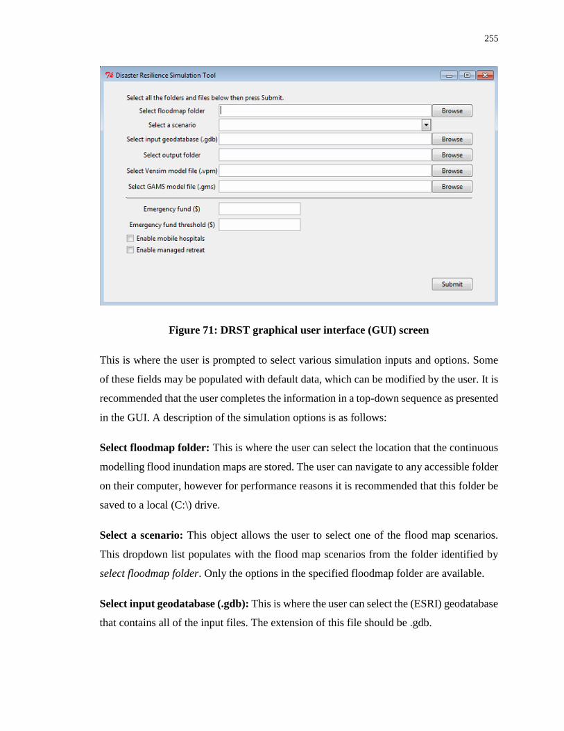
255
Figure 71: DRST graphical user interface (GUI) screen
This is where the user is prompted to select various simulation inputs and options. Some
of these fields may be populated with default data, which can be modified by the user. It is
recommended that the user completes the information in a top-down sequence as presented
in the GUI. A description of the simulation options is as follows:
Select floodmap folder: This is where the user can select the location that the continuous
modelling flood inundation maps are stored. The user can navigate to any accessible folder
on their computer, however for performance reasons it is recommended that this folder be
saved to a local (C:\) drive.
Select a scenario: This object allows the user to select one of the flood map scenarios.
This dropdown list populates with the flood map scenarios from the folder identified by
select floodmap folder. Only the options in the specified floodmap folder are available.
Select input geodatabase (.gdb): This is where the user can select the (ESRI) geodatabase
that contains all of the input files. The extension of this file should be .gdb.
256
Select output folder: This is the where the user can specify an output folder. The output
folder will contain all of the output files generated during the simulation. This is where
maps and tables will be stored. Note that if the user wishes to run multiple simulations, a
new output folder should be specified for each simulation so that files are not accidentally
overwritten.
Select Vensim model file (.vpm): This is where the user can select the Vensim model to
be run as part of the simulation. In this research, there is only one model to run, but this
input option allows the model to be stored anywhere on the user’s computer. Note that this
file is .vpm which is a published Vensim model file, and not the traditional .mdl format.
The tool comes with the published model file (.vpm), however if for any reason the user
wishes to make modifications to the Vensim model directly, the .mdl file can be opened in
Vensim, modified, and then subsequently needs to be republished (to .vpm format) before
it can be run as part of the DRST. For more information on publishing Vensim models, the
user is referred to Vensim help documentation available through the Vensim GUI or online
at: https://www.vensim.com/documentation.html.
Select GAMS model file (.gms): This is where the user can specify the location of the
GAMS model to be run as part of the simulation. In this research, there is only one model
to run, but this input option allows the user to navigate to the stored file anywhere on the
user’s computer.
The following are a set of simulation options available to the user at the beginning of the
simulation:
Emergency funds ($): This is where the user can specify the amount ($) of emergency
funding available during a simulation. The entry must be of type integer with a value
greater than or equal to zero. The format should be continuous digits with no commas, no
spaces, and no special characters. If the user wishes to make an infinite source of funding
available during a simulation, this can be proxied by entering a very large number (for
example, 999999999999). If the user wishes for no funding sources to be made available
during a simulation, then the user should enter a value of zero (0).
257
Emergency fund threshold ($): This is where the user can specify the amount ($) of
damage that triggers the use of the emergency funds during a simulation. The entry must
be of type integer with a value greater than or equal to one. The format should be
continuous digits with no commas, no spaces, and no special characters. If the user wishes
to provide access to the emergency funds immediately, the user should enter a value of one
(1). If the user does not want emergency funds to ever become available, the user can proxy
this situation by entering a very large number (for example, 999999999999).
Enable mobile hospitals: This is where the user can specify whether to implement a
mobile hospital station during a simulation. The radio button can be toggled on/off for
yes/no. If toggled off, no mobile hospitals will be added during the simulation. If toggled
on, then a mobile hospital is placed within Metro Vancouver during the simulation. The
mobile hospital will be added to the simulation at time step 6. Currently, the user does not
have control over when or where the mobile hospital is deployed during a simulation. Once
the mobile hospital is deployed, it is assumed to remain in place for the remainder of the
simulation.
Enable managed retreat: This is where the user can specify whether to implement
managed retreat during a simulation. The radio button can be toggled on/off for yes/no. If
toggled off, managed retreat does not occur during the simulation. If toggled on, then the
managed retreat of Pitt Meadows area is assumed to have taken place before the simulation
has started. Currently, the user does not have control over when or where the managed
retreat occurs during a simulation. Once managed retreat has occurred, it is assumed the
land is uninhabited for the remainder of the simulation.
Once all of the input files and folders, output locations, and simulation options have been
set, the user can press the Submit button and the simulation will proceed. The user should
not click on the interface during a simulation – this can cause instabilities which may cause
the model to crash. The user will be prompted once the simulation is complete and output
files will be saved in the output folder.
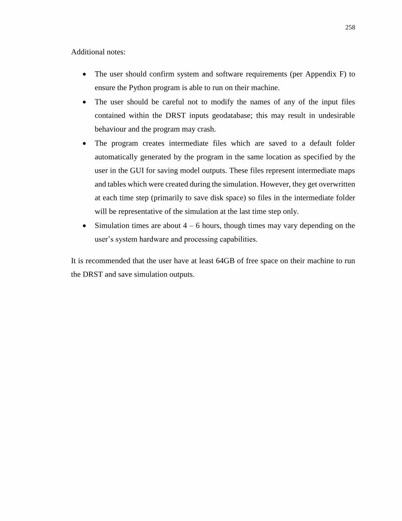
258
Additional notes:
The user should confirm system and software requirements (per Appendix F) to
ensure the Python program is able to run on their machine.
The user should be careful not to modify the names of any of the input files
contained within the DRST inputs geodatabase; this may result in undesirable
behaviour and the program may crash.
The program creates intermediate files which are saved to a default folder
automatically generated by the program in the same location as specified by the
user in the GUI for saving model outputs. These files represent intermediate maps
and tables which were created during the simulation. However, they get overwritten
at each time step (primarily to save disk space) so files in the intermediate folder
will be representative of the simulation at the last time step only.
Simulation times are about 4 – 6 hours, though times may vary depending on the
user’s system hardware and processing capabilities.
It is recommended that the user have at least 64GB of free space on their machine to run
the DRST and save simulation outputs.
259
Appendix I
Curriculum Vitae
7
Name Angela M. Peck
Post-Secondary Education The University of Western Ontario, Canada
Ph.D. Candidate
2011 – Present
The University of Western Ontario, Canada
Civil and Environmental Engineering
2011, M.E.Sc.
The University of Western Ontario, Canada
Civil and Environmental Engineering
2008, B.E.Sc.
Engineering Employment Associated Engineering (AE)
Civil Designer, Infrastructure Division
Climate Change Subject Matter Expert
2017 - Present
Awards & Achievements Alexander Graham Bell Canada Graduate Scholarship
(NSERC CGS D), Jan 2012 - Dec 2014
Nominated for Teaching Assistant Award, 2011
Ontario Graduate Scholarship (OGS), 2009 – 2010
DeMarco Family Green Technologies Award, 2008
The University of Western Ontario Entrance
Scholarship, 2004
Teaching Experience Instructor, 2017 Winter
CEE 9567b: GIS Applications to Water Resources
Management
Instructor, 2016 Winter
CEE 9567b: GIS Applications to Water Resources
Management
CEE 2219b: Computational Tools for Civil Engineers
Certificate in University Teaching and Learning,
2015 – Present

260
Completion of Advanced Teaching Program (ATP),
2015
Teaching Assistant, 2008 – 2015
Department of Civil and Environmental Engineering,
The University of Western Ontario, London, Canada
Undergraduate courses:
CEE 2218: Civil Engineering Systems
CEE 3324: Surveying
CEE 3361: Water Resources Management
CEE 4461: Natural Disasters
ES 4498: Engineering Ethics
Graduate courses:
CEE 9510: Engineering Planning and Project
Management
Specialized Training ESRI Earth Imagery at Work (2017)
ESRI Going Places with Spatial Analysis (2016)
NASA ARSET Applied Remote Sensing Training
(2016, 2018)
Publications
I. Articles published or accepted in refereed journals
Neuwirth, C., Hofer, B. and Peck, A. (2015). Spatiotemporal Processes and their
Implementation in Spatial System Dynamics Models. Journal of Spatial Science, 12pp.
Doi: 10.1080/14498596.2015.997316.
Neuwirth, C., Peck, A. and Simonovic, S.P. (2015). Modeling Structural Change in Spatial
System Dynamics: A Daisyworld Example, Environmental Modelling & Software, 65:30-
40.
Simonovic, S.P. and Peck, A. (2013). Dynamic Resilience to Climate Change Caused
Natural Disasters in Coastal Megacities – Quantification Framework. British Journal of
Environment and Climate Change, 3(3): 378-401.
Peck, A., Bowering, E. and Simonovic, S.P. (2013). A flood risk assessment to municipal
infrastructure due to changing climate part II: case study. Urban Water Journal.
Doi:10.1080/1573062X.2013.781760.
Bowering, E., Peck, A. and Simonovic, S.P. (2013). A flood risk assessment to municipal
infrastructure due to changing climate part I: methodology. Urban Water Journal.
Doi:10.1080/1573062X.2012.758293.

261
Peck, A., Prodanovic, P. and Simonovic, S.P. (2013). Rainfall Intensity Duration
Frequency Curves Under Climate Change: City of London, Ontario, Canada. Canadian
Water Resources Journal, 37(3), 177-189.
Karmakar, S., Simonovic, S.P., Peck, A., and Black, J. (2010). An Information System for
Risk-Vulnerability Assessment to Flood. Journal of Geographic Information System, 2,
129-146.
II. Other Refereed Contributions (* indicates oral presenter)
Peck, A.*, and Simonovic, S.P. (2016). Use of Resilience in Adaptation to Climate Change
Caused Natural Disasters. Adaptation Canada 2016, Ottawa, ON, April 12-14.
Peck, A.*, and Simonovic, S.P. (2015). Climate Change Influenced Riverine Flooding and
Sea Level Rise on Canada’s West Coast. Canadian Society for Civil Engineering (CSCE)
22nd Hydrotechnical Conference, Montreal, QC, April 30-May1.
Neuwirth, C.*, and Peck, A. (2013). A Conceptual Spatial System Dynamics (SSD) Model
for Structural Change in Grassland Farming. In Piantadosi, J., Anderssen, R.S., and Boland,
J. (eds) MODSIM2013, 20th International Congress on Modelling and Simulation,
Modelling and Simulation Society of Australia and New Zealand, December 2013, pp.
628-634.
Peck A.*, Bowering, E.*, and Simonovic, S.P. (2010). Assessment of Climate Change
Risk to Municipal Infrastructure: A City of London Case Study. Canadian Society for Civil
Engineering (CSCE) Annual General Meeting and Conference, 11th International
Environmental Specialty Conference, Winnipeg, MB, June 9-12.
Bowering E.*, Peck A.*, and Simonovic, S.P. (2009). A Methodology for Risk Assessment
of Municipal Infrastructure due to Climate Change: A Case Study of London, Ontario.
Proceedings of the American Geophysical Union (AGU) Annual Fall Meeting, San
Francisco, CA, December 14-18.
Peck, A.*, Black, J., Karmakar, S., and Simonovic, S.P. (2008). A Web-based Flood
Information System. CD Proceedings, 4th International Symposium on Flood Defence:
Managing Flood Risk, Toronto, Ontario, Canada, May 6-8.
III. Non-Refereed Contributions
Peck, A., Neuwirth, C. and Simonovic, S.P. (2014). Coupling System Dynamics with
Geographic Information Systems: CCaR Project Report. Water Resources Research Report
no. 086, Facility for Intelligent Decision Support, Department of Civil and Environmental
Engineering, London, Ontario, Canada, 60 pages. ISBN: (print) 978-0-7714-3069-5;
(online) 978-0-7714-3070-1.
Peck A. and Simonovic, S.P. (2013). Coastal Cities at Risk (CCaR): Generic System
Dynamics Simulation Models for Use with City Resilience Simulator. Water Resources
Research Report no. 083, Facility for Intelligent Decision Support, Department of Civil
262
and Environmental Engineering, London, Ontario, Canada, 55 pages. ISBN: (print) 978-0-
7714-3024-4; (online) 978-0-7714-3025-1.
Peck, A., Bowering, E. and Simonovic, S.P. (2011). City of London: Vulnerability of
Infrastructure to Climate Change, Final Report. Water Resources Research Report no. 074,
Facility for Intelligent Decision Support, Department of Civil and Environmental
Engineering, London, Ontario, Canada, 66 pages. ISBN: (print) 978-0-7714-2895-1;
(online) 978-0-7714-2902-6.
Peck, A., Bowering, E., and Simonovic, S.P. (2010). Draft Report (Outcome 5, 6 & 7):
Impact of Climate Change to Municipal Infrastructure: A City of London Case Study.
Project Report, the City of London, ON, September 2010.
Simonovic, S.P. and Peck, A. (2010). Updated Rainfall Intensity Duration Frequency
Curves for the City of London Under the Changing Climate. Water Resources Research
Report no. 065, Facility for Intelligent Decision Support, Department of Civil and
Environmental Engineering, London, Ontario, Canada. ISBN: (Print) 978-0-7714-2819-7;
(Online) 978-0-7714-2820-3.
Bowering, E., Peck, A., and Simonovic, S.P. (2009) Status Report 1 – Project Definition
Report. The City of London, ON. March 2009.
Peck, A., Karmakar, S., and Simonovic, S.P. (2007). Physical, Economical, Infrastructural
and Social Flood Risk - Vulnerability Analyses in GIS. Water Resources Research Report
no. 057, Facility for Intelligent Decision Support, Department of Civil and Environmental
Engineering, London, Ontario, Canada. ISBN: (Print) 978-0-7714-2662-9; (Online) 978-
0-7714-2663-6.
IV. Other Contributions
Keynote Speaker, 5th International Conference on Geoinformation Technologies for
Natural Disaster Management (GiT4NDM). Mississauga, Ontario, October 9-11, 2013.
Panel Member, Translating Climate Model Outputs into Engineering Parameters for the
Transportation Sector, Climate Adaptation Futures: Second International Climate Change
Adaptation Conference 2012. Tucson, AZ, May 29-31, 2012.