a dynamical study of the friedmann equationscds.cern.ch/record/515592/files/0108066.pdfa dynamical...

A Dynamical Study of the Friedmann Equations

Jean-Philippe Uzan† and Roland Lehoucq‡

†Laboratoire de Physique Theorique, CNRS–UMR 8627,Bat. 210, Universite Paris XI, F–91405 Orsay (France)‡CE-Saclay/DSM/DAPNIA/Service d’Astrophysique,F–91191 Gif sur Yvette cedex (France).

Abstract. Cosmology is an attracting subject for students but usually difficult todeal with if general relativity is not known. In this article, we first recall the Newtonianderivation of the Friedmann equations which govern the dynamics of our universe anddiscuss the validity of such a derivation. We then study the equations of evolution ofthe universe in terms of a dynamical system. This sums up the different behaviors ofour universe and enables to address some cosmological problems.

PACS numbers: ???

1. Introduction

In this article, we want to present a pedagogical approach to the equations governing the

evolution of the universe, namely the Friedmann equations. Indeed, the derivation of

this equations is intrinsically relativistic. Although in Newtonian theory, the universe

must be static, Milne [1] and McCrea and Milne [2] showed that, surprisingly, the

Friedmann equations can be derived from the simpler Newtonian theory. In section 2,

we recall their derivation (§ 2.1) for a universe filled with pressureless matter and then

discuss the introduction of a cosmological constant (§ 2.2). Indeed, it is puzzling that

the Newtonian theory and general relativity give the same results; we briefly discuss

this issue in § 2.3.

Once we have interpreted the Friedmann equations, we study them as a dynamical

system. The first authors to consider such an approach were Stabell and Refsdal [3]

who investigated the Friedmann–Lemaıtre model with a pressureless fluid. This was

then generalised to a fluid with any equation of state [4, 5]. Then, this technique

was intensively used to study the isotropisation of homogeneous models (see e.g. [6]

and references therein). For a general description of the use of dynamical systems in

cosmology, we refer to the book by Wainwright and Ellis [7] where most of the techniques

are detailed. Our purpose here, is to present such an analysis for a fluid with any

equation of state and including a cosmological constant while staying as pedagogical

as possible. In section § 3, we rewrite the Friedmann equations under a form easier

to handle with and we extract the dynamical system to study. We then determine the

A Dynamical Study of the Friedmann Equations 2

fixed points of this system and discuss their stability. We illustrate this analytic study

by a numerical integration of this set of equations (§ 4) and finish by a discussion about

the initial conditions explaining the current observed state of our universe (§ 5).

2. A Newtonian derivation of the Friedmann equation

We follow the approach by Milne [1] and McCrea and Milne [2] and the reader is referred

to [8] for further details.

2.1. General derivation

We consider a sphere of radius R filled with a pressureless fluid (P = 0) of uniform

(mass) density ρ free–falling under its own gravitational field in an otherwise empty

Euclidean space. We decompose the coordinate x of any particle of the fluid as

x = a(t)r (1)

where r is a constant vector referred to as the comoving coordinate, t is the time

coordinate and a the scale factor. We choose a to have the dimension of a length

and r to be dimensionless. It implies that the sphere undergoes a self similar expansion

or contraction and that no particle can cross another one. Indeed the edge of the sphere

is also moving as

R(t) = a(t)R0. (2)

Assume that while sitting on a particle labelled i we are observing a particle labelled j;

we see it drift with the relative velocity

vij = a (rj − ri) = Hxij (3)

where a dot refers to a time derivative, H ≡ a/a and xij ≡ (rj − ri). As a consequence,

any particle i sees any other particle j with a radial velocity proportional to its distance

and the expansion is isotropic with respect to any point of the sphere, whatever the

function a(t). But, note that this does not imply that all particles are equivalent (as

will be discussed later).

To determine the equation of motion of any particle of this expanding sphere, we

first write the equation of matter conservation stating that the mass within any comoving

volume is constant (i.e. ρx3 ∝ r3) implying that

ρ(t) ∝ a−3(t), (4)

which can also be written under the form

ρ + 3Hρ = 0. (5)

Note that Eq. (5) can also be deduced from the more general conservation equation

∂tρ +∇xj = 0 with j = ρv, v = Hx and ∇xx = 3.


To determine the equation of evolution of the scale factor a, we first compute the

gravitational potential energy EG of a particle of masse m by applying the Gauss law

EG = −GM(< x)m

x(6)

where G is the Newton constant and M(< x) the mass within the sphere of radius x

given by

M(< x) =4π

3ρx3. (7)

We then need to evaluate its kinetic energy EK which takes the simple form

EK =1

2mx2. (8)

The conservation of the total energy E = EG + EK implies, after the use of the

decomposition (1) and a simplification by r, that(a

a

)2

=8πG

3ρ− Kc2

a2(9)

where K is a dimensionless constant (which can depend on r) given by K =

−2E/(mc2r2)‡.

2.2. Introducing a cosmological constant

In the former derivation, the gravitational potential on any particle inside the sphere is

proportional to the distance x2. Any other force deriving from a potential proportional

to x2 will mimic a gravitational effect. A force deriving from the potential energy EΛ

defined by

EΛ = −mΛc2

6x2 (10)

where Λ is a constant was introduced by Einstein in 1917. As in the previous section,

writing that the total energy E = EK + EG + EΛ is constant leads to the equation of

motion (a

a

)2

=8πG

3ρ− Kc2

a2+

Λc2

3. (11)

From (10), we deduce that Λ has the dimension of an inverse squared length. The total

force on a particle is

F = m

(−4πG

3ρ +

Λc2

3

)x (12)

from which it can be concluded that (i) it opposes gravity if Λ is positive and that (ii)

it can be tuned so that F = 0 leading to a = 0 and ρ =constant if

Λ =4πG

c2ρ. (13)

‡ This scaling of K with r is imposed by the requirement that the expansion is self–similar (Eq. 1) andthat no shell of labeled r can cross a shell of label r′ > r.


Table 1. Units of the quantities introduced in the article. M , L and T standrespectively for mass, length and time units.

a r v ρ P E H Λ K

L − L.T−1 M.L−3 M.L−1.T−2 M.L2.T−2 T−1 L−2 −

This enables to recover a static autogravitating sphere hence leading to a model for a

static universe. The force deriving from EΛ is analogous to the one exerted by a spring

of negative constant.

To finish, we recall on table 1 the dimension of all the quantities used in the former

sections, mainly to compare with standard textbooks in which the choice c = 1 is usually

made.

2.3. Discussion

From this Newtonian approach, the equation of evolution of the universe identified

with this gravitating sphere are thus given by equation (5) and (11). These are two

differential equations for the two variables a(t) and ρ(t) which can be solved once the

two parameters K and Λ have been chosen.

In the context of general relativity, one can deduce the law of evolution for the scale

factor of the universe a which is given by the Friedmann equations

H2 =κ

3ρ− Kc2

a2+

Λc2

3(14)

a

a= − κ

6(ρ + 3

P

c2) +

Λc2

3(15)

with κ ≡ 8πG and the conservation equation

ρ + 3H(ρ +P

c2) = 0. (16)

Eq. (14) reduces to (11) and, Eq. (16) to (5) when P = 0. The equation (15) is

redundant and can be deduced from the two others. Note that now Eq. (16) is also a

conservation equation but with the mass flux j = (ρ + P/c2)v. This can be interpreted

by remembering that the first law of thermodynamics for an adiabatic system [9] takes

the form

E + P V = 0 (17)

where E = ρV c2 is the energy contained in the physical volume V (scaling as a3).

The first thing to stress is that equations (5) and (11) do not depend on the radius

R0 of the sphere. It thus seems that we can let it go to infinity without changing the

conclusions and hence explaining why we recover the Friedmann equations. This was

the viewpoint adopted by Milne [1] and McCrea and Milne [2]. This approach leads to

some problems. First, it has to be checked that the Gauss theorem still applies after

taking the limit toward infinity (i.e. one has to check that the integrals and the limit


commute). This imposes that ρ decreases fast enough with r and thus that there is

indeed a center. Equivalently, as pointed out by Layzer [10], the force on any particle

of an infinite homogeneous distribution is undetermined (the integral over the angles

is zero while the integral over the radial coordinate is infinite). The convergence of

the force requires either the mass distribution to be finite (in which case it can be

homogeneous) or to be inhomogeneous if it is infinite. The issue of the finiteness of the

universe has been widely discussed and a clear presentation of the evolution of ideas in

that respect are presented in [16]. Second, for distances of cosmological interests, i.e. of

some hundred of Megaparsec, the recession speed of the particles of the sphere are of

order of some fraction of the speed of light. One will thus require a (special) relativistic

treatment of the expanding sphere. Third, the gravitational potential grows with the

square of the radius of the sphere but it can not become too large otherwise, due to the

virial theorem, the velocities would exceed the speed of light.

It was then proposed [12] that such an expanding sphere may describe a region

the size of which is small compared with the size of the observable universe (i.e. of the

Hubble size). Since all regions of a uniform and isotropic universe expand the same way,

the study of a small region gives information about the whole universe (but this does

not solve the problem of the computation of the gravitational force).

The center seems to be a privileged points since it is the only point to be at rest

with respect to the absolute frame. But, one can show that the spacetime background of

Newtonian mechanics is invariant under a larger group than the traditionally described

Galilean group. As shown by Milne [1], McCrea and Milne [2] and Bonnor [13] (see also

Carter and Gaffet [14] for a modern description) it includes the set of all time-dependent

space translations

xi → xi + zi(t)

where zi(t) are arbitrarily differentiable functions depending only on the time coordinate

t. This group of transformation is intermediate between the Galilean group and the

group of all diffeomorphisms under which the Einstein theory in invariant. Thanks to

this invariance group, each point can be chosen as a center around which there is local

isotropy and homogeneity but the isotropy is broken by the existence of the boundary

of the sphere (i.e. all observer can believe living at the center as long as he/she does

not observe the boundary of the expanding sphere).

There are also conceptual differences between the Newtonian cosmology and the

relativist cosmology. In the former we have a sphere of particle moving in a static and

absolute Euclidean space and the time of evolution of the sphere is disconnected from

the absolute time t. For instance in a recollapsing sphere, the time will go on flowing

even after the crunch of the sphere. In general relativity, space is expanding and the

particles are comoving. We thus identify an expanding sphere in a fixed background

and an expanding spacetime with fixed particles. As long as we are dealing with a

pressureless fluid, this is possible since there is no pressure gradient and each point of

the sphere can be identify with one point of space (in fact, with an absolute time we are

working in a synchronous reference frame and we want it to be also comoving, which is


Table 2. Comparison of the nature of the Newtonian trajectory and of the structureof space according to the value of the constant K in Eq. (11).

E > 0 0 < 0

Trajectory hyperbolic parabolic ellipticunbounded unbounded bounded

K < 0 0 > 0

Spatial section infinite infinite finite

possible only if P = 0 [15]). Moreover, the pressure term in the Friedmann equations

cannot trivially be recovered from the Newtonian argument. As shown, one gets the

correct Friedmann equations if one starts from the conservation law including pressure

(and derived from the first law of thermodynamics) and the conservation of energy. But

if one were starting from the Newton law relating force (12) and acceleration (max), the

term containing the pressure in (15) would not have been recovered; one should have

added an extra pressure contribution FP = −4πGmPx/c2 which can not be guessed.

This is a consequence that in general relativity any type of energy has a gravitational

effect. In a way it is a “miracle” that the equation (14) does not depend on P , which

makes it possible to derive from the Newtonian conservation of energy. Beside it has also

to be stressed that the Newtonian derivation of the Friedmann equations by Milne came

after Friedmann and Lemaıtre demonstrated the validity of the Friedmann equations

for an unbounded homogeneous distribution of matter (using general relativity). It has

to be pointed out that these Newtonian models can not explain all the observational

relations since, contrary to general relativity, they do not incorporate a theory of light

propagation. As outlined by Lazer [10] one can sometime legitimately treat a part

of the (dust) expanding universe as an isolated system in which case the Newtonian

treatment is correct, which makes McCrea [11] conclude that this is an indication that

Einstein’s law of gravity must admit the same interpretation as that of Newton’s in the

case of a spherically symmetric mass distribution. Note that the structural similarity of

Einstein and Newton gravity were put forward by Cartan [17] who showed that these

two theories are much closer that one naively thought and, in that framework (which

goes far beyond our purpose) one can work out a correct derivation of the Friedmann

equations (see e.g. [18]).

The most important outcome of the Newtonian derivation of the Friedmann

equations is that it allows to interpret equation (14) in terms of the conservation of

energy; the term in H2 represents the kinetic energy, the term in κρ/3 the gravitational

potential energy, the term in Λ/3 the energy associated with the cosmological constant

and the term in K the total energy of the system. The properties of the spatial sections

(i.e. of the three dimensional spaces of constant time) are related to the sign of K and

can be compared with the property of the trajectories of the point of the sphere which

are related to the sign of the total energy E; we sum up all these properties on table 2.


3. The Friedmann equations as a dynamical system

The Friedmann equations (14–15) and the conservation equation (16) form a set of two

independent equations for three variables (a, P and ρ). The usual approach is to solve

this system by specifying the matter content of the universe mainly by assuming an

equation of state of the form

P = (γ − 1)ρc2 (18)

where γ may depend on ρ and thus on time. For a pressureless fluid (modelling

for instance a fluid of galaxies) γ = 1 and for a fluid of radiation (such as photon,

neutrino,...) γ = 4/3. We assume that γ 6= 0 since such a type of matter is described

by the cosmological constant and singled out from “ordinary” matter and that γ 6= 2/3

since such a type of matter mimics the curvature term and is thus incorporated with it.

One can then first integrate (16) rewritten as dρ/(γρ) = −3da/a to get the function

ρ(a) which, in the case where γ is constant, yields

ρ(a) = Ca−3γ (19)

where C is a positive constant of integration, and then insert the solution for ρ(a) in

Eq. (14) to get a closed equation for the scale factor a (see e.g. [19] for such an approach

and [20] for an alternative and pedagogical derivation).

In this section, we want to present another approach in which the Friedmann

equations are considered as a dynamical system and to determine its phase space.

3.1. Derivation of the system

The first step is to rewrite the set of dynamical equations with the three new variables

Ω, ΩΛ and ΩK defined as

Ω ≡ κρ

3H2, (20)

ΩΛ ≡ Λc2

3H2, (21)

ΩK ≡ − Kc2

a2H2. (22)

They respectively represent the relative amount of energy density present in the matter

distribution, cosmological constant and curvature. Ω has to be positive and there is no

constraint on the sign of both ΩΛ and ΩK . With these definitions, it is straightforward

to deduce from (14) that

Ω + ΩΛ + ΩK = 1. (23)

Using that H = a/a − H2, expressing a/a from Eq. (15) and H2 from Eq. (14), we

deduce that

H

H2= −(1 + q) (24)


where the deceleration parameter q is defined by

q ≡ 3γ − 2

2(1− ΩK)− 3γ

2ΩΛ. (25)

It is useful to rewrite the full set of equations by introducing the new dimensionless time

variable η ≡ ln(a/a0), a0 being for instance the value of a today. The derivative of any

quantity X with respect to η, X ′, is then related to its derivative with respect to t by

X ′ = X/H. The equation of evolution of the Hubble parameter (24) takes the form

H ′ = −(1 + q)H. (26)

Now, differentiating Ω, ΩΛ and ΩK with respect to η, using Eq. (26) to express H ′,a′ = a and Eq. (16) to express ρ′ = −3γρ, we obtain the system

Ω′ = (2q + 2− 3γ)Ω (27)

Ω′Λ = 2(1 + q)ΩΛ (28)

Ω′K = 2qΩK (29)

and it is trivial to check that Ω′ + Ω′Λ + Ω′

K = 0 as expected form (23).

Indeed, it is useless to study the full system (26–29) (i) since H does not enter the

set of equations (27–29) and is solely determined by Eq. (26) once this system has been

solved and (ii) since Ω can be deduced algebraically from (23). As a consequence, we

retain the closed systemΩ′

Λ = 2(1 + q)ΩΛ

Ω′K = 2qΩK

(30)

with q being a function of ΩΛ and ΩK only and defined in (25).

The system (30) is autonomous [21], which implies that there is a unique integral

curve passing through a given point, except where the tangent vector is not defined

(fixed points). Note that at every point on the curve the system (30) assigns a unique

tangent vector to the curve at that point. It immediately follows that two trajectories

cannot cross; otherwise the tangent vector at the crossing point would not be unique [21].

3.2. Determination of the fixed points

To study the system (30) as a dynamical system, we first need to determine the set of

fixed points, i.e. the set of solutions such that Ω′Λ = 0 and Ω′

K = 0. These solutions

represent equilibrium positions which indeed can be either stable or unstable. The fixed

points are thus solutions of

(1 + q)ΩΛ = 0, qΩK = 0. (31)

We obtain the three solutions

(ΩK , ΩΛ) ∈ (0, 0), (0, 1), (1, 0) . (32)

Each of these solutions represent a universe with different physical characteristics:


(i) (ΩK , ΩΛ) = (0, 0): the Einstein de Sitter space (EdS).

It is a universe with flat spatial sections, i.e. the three dimensional hypersurfaces of

constant time are Euclidean and it has no cosmological constant. We deduce from

(23) and (25) that

Ω = 1, q =3

2γ − 1 (33)

and integrating Eq. (14) gives

a(t) =

√

κC

3t

23γ

(34)

for the solution vanishing at t = 0.

(ii) (ΩK , ΩΛ) = (0, 1): the de Sitter space (dS).

It is an empty space filled with a positive cosmological constant and with flat spatial

sections. We deduce from (23) and (25) that

Ω = 0, q = −1 (35)


a(t) = a0e√

Λ3

t. (36)

This universe is accelerating in an eternal exponential expansion.

(iii) (ΩK , ΩΛ) = (1, 0): the Milne universe (M).

It is an empty space with no cosmological constant and with hyperbolic spatial

section (K < 0). We deduce from (23) and (25) that

Ω = 0, q = 0 (37)


a(t) = a0t (38)

for the solution vanishing at t = 0 and in units where K = a20.

It is also interesting to study the properties of the three following invariant lines

which separate the phase space in disconnected regions:

(i) ΩK = 0: The system (30) reduces to the equation of evolution for ΩΛ

Ω′Λ = 3γ(1− ΩΛ)ΩΛ. (39)

Thus, if initially ΩK = 0, we stay on this line during the whole evolution and

converge toward either ΩΛ = 1 (i.e. the fixed point dS) or toward ΩΛ = 0 (i.e. the

fixed point EdS). It also follows that no integral flow lines of the system (30) can

cross the line ΩK = 0. It separates the universes with ΩK > 0 which are compact

(i.e. having a finite spatial extension) and the universes with ΩK < 0 which are

infinite (if one assumes trivial topology [23]). Crossing the line ΩK = 0 would thus

imply a change of topology. Note that if γ = 0, the fluid behaves like a cosmological

constant and thus Ω′Λ = 0 since ΩK remains zero.


(ii) ΩΛ = 0: The system (30) reduces to the equation of evolution for ΩK

Ω′K = (3γ − 2)(1− ΩK)ΩK . (40)

As in the previous case, we stay on this line during the whole evolution and converge

toward either ΩK = 1 (i.e. the fixed point M) or toward ΩΛ = 0 (i.e. the fixed

point EdS). It also follows that no integral flow lines of the system (30) can cross

the line ΩΛ = 0. Note that if γ = 2/3, the fluid behaves like a curvature term and

thus Ω′K = 0 since ΩΛ remains zero.

(iii) Ω = 0: It is a boundary of the phase space since Ω is non negative. We now have

q = −ΩΛ and the system (30) reduces to

Ω′Λ = 2(1− ΩΛ)ΩΛ. (41)

The universe converges either toward (dS) or (M).

3.3. Stability analysis

The second step is to determine whether these fixed points are stable (i.e. attractors:

A), unstable (i.e. repulsor: R) or saddle (S) points (i.e. attractor in a direction and

repulsor in another). This property can be obtained by studying at the evolution of a

small deviation from the equilibrium configuration. We thus decompose ΩK and ΩΛ as

ΩK ≡ ΩK + ωK , (42)

ΩΛ ≡ ΩΛ + ωΛ , (43)

where (ΩΛ, ΩK) represents the coordinates of one of the fixed points determined in the

previous section and where (ωΛ, ωK) is a small deviation around this point.

Writing the system of evolution (30) as(ΩK

ΩΛ

)′=

(FK(ΩΛ, ΩK)

FΛ(ΩΛ, ΩK)

), (44)

where FK and FΛ are two functions determined from (30), it can be expanded to linear

order around (ΩK , ΩΛ) (for which FK and FΛ vanish) to give the equation of evolution

of (ωΛ, ωK) (ωK

ωΛ

)′=

∂FK

∂ΩK

∂FK

∂ΩΛ∂FΛ

∂ΩK

∂FΛ

∂ΩΛ

(ΩΛ,ΩK)

(ωK

ωΛ

)≡ P(ΩΛ,ΩK)

(ωK

ωΛ

). (45)

The stability of a given fixed point depends on the sign of the two eigenvalues (λ1,2) of the

matrix P(ΩΛ,ΩK). If both eigenvalues are positive (resp. negative) then the fixed point is a

repulsor (resp. an attractor) since (ωK , ωΛ) will respectively goes to infinity (resp. zero).

In the case where the two eigenvalues have different signs, the fixed point is an attractor

along the direction of the eigenvector associated with the negative eigenvalue and a

repulsor along the direction of the eigenvector associated with the positive eigenvalue.

We also introduce uλ1,2 the eigenvectors associated to the two eigenvalues which give

the (eigen)–directions of attraction or repulsion.


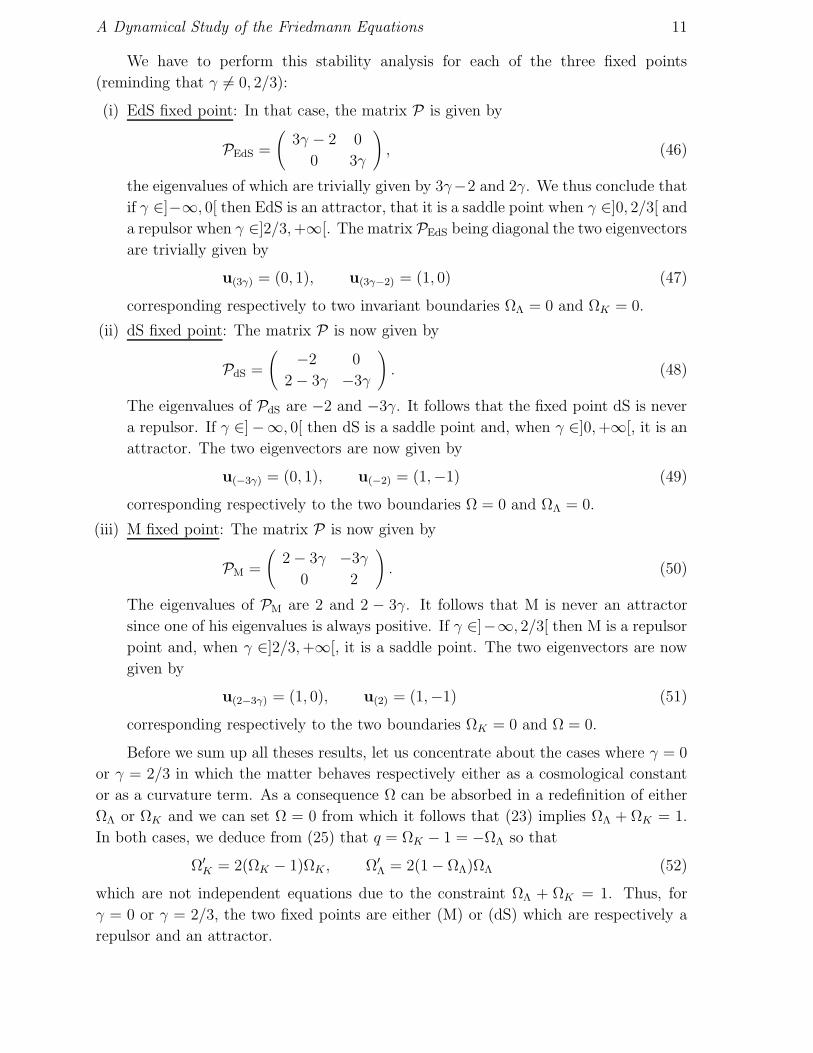
We have to perform this stability analysis for each of the three fixed points

(reminding that γ 6= 0, 2/3):

(i) EdS fixed point: In that case, the matrix P is given by

PEdS =

(3γ − 2 0

0 3γ

), (46)

the eigenvalues of which are trivially given by 3γ−2 and 2γ. We thus conclude that

if γ ∈]−∞, 0[ then EdS is an attractor, that it is a saddle point when γ ∈]0, 2/3[ and

a repulsor when γ ∈]2/3, +∞[. The matrix PEdS being diagonal the two eigenvectors

are trivially given by

u(3γ) = (0, 1), u(3γ−2) = (1, 0) (47)

corresponding respectively to two invariant boundaries ΩΛ = 0 and ΩK = 0.

(ii) dS fixed point: The matrix P is now given by

PdS =

( −2 0

2− 3γ −3γ

). (48)

The eigenvalues of PdS are −2 and −3γ. It follows that the fixed point dS is never

a repulsor. If γ ∈]−∞, 0[ then dS is a saddle point and, when γ ∈]0, +∞[, it is an

attractor. The two eigenvectors are now given by

u(−3γ) = (0, 1), u(−2) = (1,−1) (49)

corresponding respectively to the two boundaries Ω = 0 and ΩΛ = 0.

(iii) M fixed point: The matrix P is now given by

PM =

(2− 3γ −3γ

0 2

). (50)

The eigenvalues of PM are 2 and 2 − 3γ. It follows that M is never an attractor

since one of his eigenvalues is always positive. If γ ∈]−∞, 2/3[ then M is a repulsor

point and, when γ ∈]2/3, +∞[, it is a saddle point. The two eigenvectors are now

given by

u(2−3γ) = (1, 0), u(2) = (1,−1) (51)

corresponding respectively to the two boundaries ΩK = 0 and Ω = 0.

Before we sum up all theses results, let us concentrate about the cases where γ = 0

or γ = 2/3 in which the matter behaves respectively either as a cosmological constant

or as a curvature term. As a consequence Ω can be absorbed in a redefinition of either

ΩΛ or ΩK and we can set Ω = 0 from which it follows that (23) implies ΩΛ + ΩK = 1.

In both cases, we deduce from (25) that q = ΩK − 1 = −ΩΛ so that

Ω′K = 2(ΩK − 1)ΩK , Ω′

Λ = 2(1− ΩΛ)ΩΛ (52)

which are not independent equations due to the constraint ΩΛ + ΩK = 1. Thus, for

γ = 0 or γ = 2/3, the two fixed points are either (M) or (dS) which are respectively a

repulsor and an attractor.


Table 3. Stability properties of the three fixed points (EdS, dS and M) as a functionof the polytropic index γ. (A: attractor, R: repulsor and S: saddle point)

γ ]−∞, 0[ 0 ]0, 2/3[ 2/3 ]2/3, +∞[

EdS A N.A. S N.A. RdS S A A A AM S R R R S

(c)

Ω=0Ω

Ω

ΩΩ=0

Ω

ΩΩ=0

Ω Λ ΛΛ

K K K

EdS EdSEdS

M M M

dS dS dS

(a) (b)

Figure 1. The fixed points and their stability depending of the value of the index γ:(a) γ < 0, (b) 0 ≤ γ < 2/3 and (c) γ ≥ 2/3.

As a conclusion of this study, we sum up the properties of the three spacetimes

as a function of the polytropic index of the cosmic fluid in table 3 and in figure 1,

we depict the fixed points, their directions of stability and instability as well as the

invariant boundary in the plane (ΩΛ, ΩK). Indeed, the attractor solution can be guessed

directly from Eq. (14) and the behavior (19) of the density with the scale factor since

if γ < 0 the matter energy density scales as a−3γ and comes to dominate over the

cosmological constant (scaling as a0) and the curvature (scaling as a−2). On the other

hand the cosmological constant always finishes by dominating if γ > 0. The curvature

can never dominates in the long run since it will be caught up by either the matter or

the cosmological constant.

4. Numerical examples

The full phase space picture can be obtained only through a numerical integration of

the system (30) by using an implicit fourth order Runge–Kutta method [22].

Ordinary matter such as a pressureless fluid or a radiation fluid has γ > 1 and we

first consider this case on figure 2 where we depict the phase space both in the (ΩK , ΩΛ)


- 1

-0,5

0

0,5

1

-0,5 0 0,5 1 1,5

ΩK

ΩΛ

Ω < 0

0

0,5

1

1,5

2

-0,5 0 0,5 1 1,5

Ω

ΩΛ

ΩK = 0

Figure 2. Phase space of the system (30) in the plane (ΩK , ΩΛ) [left] and (Ω, ΩΛ)[right]. We have represented the three fixed points and the lines ΩK = 1 and ΩΛ = 1and we have considered the value γ = 1 (i.e. pressureless fluid).

-0,2

0

0,2

0,4

0,6

0,8

1

-0,2 0 0,2 0,4 0,6 0,8 1

ΩK

ΩΛ

Ω < 0

0

0,2

0,4

0,6

0,8

1

1,2

1,4

-0,4 -0,2 0 0,2 0,4 0,6 0,8 1

Ω

ΩΛ

Figure 3. Phase space of the system (30) in the plane (ΩK , ΩΛ) [left] and (Ω, ΩΛ)[right] for γ = 1/3.

where the analytic study of the fixed points was performed but also in the plane (Ω, ΩΛ)

for complementarity. On figure 3, we consider the case where 0 < γ < 2/3 which can

corresponds to a scalar field slowly rolling down its potential or a tangle of domain

strings (for which γ = 1/3) and we finish by the more theoretical case where γ < 0 on

figure 4 for which we know no simple physical example (see however [30]).


-0,5

0

0,5

1

-0,5 0 0,5 1

ΩK

ΩΛ

Ω < 0

0

0,2

0,4

0,6

0,8

1

1,2

1,4

-0,4 -0,2 0 0,2 0,4 0,6 0,8 1

Ω

ΩΛ

ΩK = 0

Figure 4. Phase space of the system (30) in the plane (ΩK , ΩΛ) [left] and (Ω, ΩΛ)[right] for γ = −1.

5. Discussion and conclusions

To discuss the naturalness of the initial conditions leading to our observed universe, we

have to add the actual observational measures in the plane (Ω, ΩΛ) and trace them back

to estimate the domain in which our universe has started. This required (i) to know

what are the constraints on the cosmological constant and the curvature of the universe

and (ii) determine the age of the universe, i.e. the time during which we must integrate

back.

It is not the purpose of this article to detail the observational methods used in

cosmology and a description can be found en e.g. [19]; we now just sum up what is

thought to be the current status of these observations. The current observational data

such as the cosmic microwave background measurements [24], the Type Ia supernovae

data [25], large scale velocity fields [26], gravitational lensing [27] and the measure of

the mass to light ratio [28] tend to show that

Ω0 ∼ 0.3, ΩΛ0 ∼ 0.7. (53)

We refer the reader to the review by Bahcall et al. [29] for a combined study of these

data and a description of all the observation methods. Let us just keep in mind that we

are close to the line ΩK = 0 and let us consider the safe area of parameter such that

D0 : Ω0 ∈ [0.1, 0.5], ΩΛ0 ∈ [0.5, 0.9] (54)

and let us determinate the initial conditions allowed by these observations.

For that purpose, we need to integrate the system (30) back in time during a time

equal to the age of the universe. Today, the matter content of the universe is dominated

by a pressureless fluid, the energy density of which is obtained once Ω0 has been chosen


and is

ρmat =3H2

0

κΩ0

(a

a0

)−3

= 1.80× 10−29Ω0 h2(

a

a0

)−3

g.cm−3 (55)

where H0 = 100 h km/s/Mpc is the Hubble constant today. The energy density of

the radiation is obtained by computing the energy contained in the cosmic microwave

background which is the dominant contribution to the radiation in the universe. Since it

is a black body with temperature Θ0 = 2.726 K, we deduce, from the Stephan-Boltzmann

law, that

ρrad = 4.47(1 + fν)× 10−34(

a

a0

)−4

g.cm−3 (56)

where fν = 0.68 is a factor to take into account the contribution of three families of

neutrinos [19]. The radiation was thus dominating over the matter for scale factors

smaller than aeq at which ρmat = ρrad and thus given by

aeq

a0' 4.5× 10−5

Ω0 h2. (57)

We can integrate back until the Planck era for which aPl/a0 ∼ 10−30 and can thus

approximate γ by

γ =

1 aeq ≤ a ≤ a0

4/3 aPl ≤ a ≤ aeq(58)

which is a good approximation for γ = 1 + 1/3(1 + a/aeq). In figure 5, we depict the

domain D0 of current observational values and its inverse image by the system (30) at

the beginning of the matter era and at the end Planck era.

To illustrate this fine tuning problem analytically, let us just consider the simplest

case where ΩΛ = 0 for which the evolution of Ω is simply given by

Ω′ = (3γ − 2)Ω(Ω− 1) (59)

the solution of which is

Ω =1

1 +ΩK0

Ω0

(aa0

)3γ−2 (60)

and thus,

Ω =

1

1+ΩK0Ω0

aa0

aeq ≤ a ≤ a0

1

1+ΩK0Ω0

a0aeq

(a

a0

)2 aPl ≤ a ≤ aeq.. (61)

From the observational data we get that ΩK0 ∼ O(10−1) and thus Ω0 ∼ O(1) from

which we deduce that

ΩK |a=aeq∼ O(10−4), ΩK |a=aPl

∼ O(10−58). (62)

This illustrate that a almost flat universe requires a fine tuning of the curvature, which

is a consequence that ΩK = 0 is a repulsor in both the radiation and the matter era.


0

0,2

0,4

0,6

0,8

1

1,2

0 0,2 0,4 0,6 0,8 1

ΩΛ

ΩΩ

K = 0

0

0,2

0,4

0,6

0,8

1

1,2

0 0,2 0,4 0,6 0,8 1

ΩΛ

Ω

ΩK = 0

z = 5

z = 1

z = 0

z = 3

Figure 5. The domain D0 of current observational values for our universe and itsinverse image by the system (30) when one is assuming that the universe has beendominated by a pressureless fluid during its whole evolution.

A solution to solve this fine tuning problem would be to add a phase prior to the

radiation era in which γ ≤ 0 so that ΩK = 0 becomes an attractor and to tune the

duration of this era such as to have the correct initial conditions. Then, during the

standard evolution EdS becomes repulsor and we evolve toward dS staying close to the

line ΩK = 0 hence explaining current observations. Inflation is a realisation of such

a scenario. What inflation really does is to change the stability property of the fixed

points and invariant boundaries of the system (30). Hence during this period where a

fluid with negative pressure is dominating we are attracted close to the line ΩK = 0 and

the closer the longer this phase lasts. We then switch to a phase with normal matter and

start to drift away due to repulsive property of EdS. Nevertheless, inflation does more

than just explaining where we stand in this phase space, it also gives an explanation

for the observed structures (galaxies, clusters...) of our universe, but this is beyond the

scope of this article.

Acknowledgments

We thank Lucille Martin and Jean-Pierre Luminet for discussions and Brandon Carter

for clarification concerning the invariance of Newtonian mechanics. JPU dedicates this

work to Yakov.

[1] E. Milne, “A Newtonian expanding universe”, Quarterly J. of Math. 5 (1934) 64.[2] W.H. McCrea and E. Milne, “Newtonian universes and the curvature of space”, Quarterly J. of

Math. 5 (1934) 73.


[3] R. Stabell and S. Refsdal, “Classification of general relativistic world models”, Mon. Not. R.Astron. Soc. 132 (1966) 379.

[4] M.S. Madsen and G.F.R. Ellis, Mon. Not. R. Astron. Soc. 234 (1988) 67.[5] M.S. Madsen, J.-P. Minoso, J.A. Butcher, and G.F.R. Ellis, Phys. Rev. D46 (1992) 1399.[6] M. Goliath and G.F.R. Ellis, “Homogeneous cosmology with a cosmological constant”, Phys. Rev.

D60 (1999) 023502.[7] J. Wainwright and G.F.R. Ellis, Dynamical systems in Cosmology, (Cambridge University Press,

Cambridge, 1997).[8] E.P. Harrison, Cosmology: the science of the universe (Cambridge University Press, Cambridge,

2000).[9] R.C. Tolman, Relativity, thermodynamics and cosmology, (Clarendon Press, Oxford, 1934).

[10] D. Layzer, “On the significance of Newtonian cosmology”, Astron. J. 59 (1954) 268.[11] W.H. McCrea, “On the significance of Newtonian cosmology”, Astron. J. 60 (1955) 271.[12] C. Callan, R.H. Dicke, and P.J.E. Peebles, “Cosmology and Newtonian Dynamics”, Am. J. Phys.

33 (1965) 105.[13] W.B. Bonnor, “Jean’s formula for gravitational instability”, Mon. Not. R. Astron. Soc. 117 (1957)

104.[14] B. Carter and B. Gaffet, “Standard covariant formulation for perfect fluid dynamics”, J. Fluid

Mech. 186 (1987) 1.[15] L. Landau and E. Lifchitz, Theorie des champs, (Mir, Moscow, 1989).[16] E.P. Harrison, “Newton and the infinite universe”, Physics Today 39 (1986) 24.[17] E. Cartan, Ann. Sci. de l’Ecole Normale Superieure 40 (1923) 325; ibid, 41 (1924) 1.[18] C Ruede and N. Straumann, “On Newton–Cartan Cosmology”, [gr-qc/9604054].[19] P.J.E. Peebles, Principles of Physical Cosmology (Princeton Series in Physics, Princeton, New

Jersey, 1993).[20] V. Faraoni, “Solving for the dynamics of the universe”, Am. J. Phys. 67 (1999) 732.[21] C. Bender and S. Orszag, Advanced Mathematical Methods for Scientists and Engineers, McGraw-

Hill International Editions[22] W. Press, S. Teukolsky, W. Vetterling and B. Flannery, Numerical Recipes 2nd edition, Cambridge

University Press.[23] M. Lachieze–Rey and J.–P. Luminet, “Cosmic Topology”, Phys. Rep. 254 (1995) 135; J-P. Uzan,

“What do we know and what can we learn about the topology of the universe?”, Int. Journalof Theor. Physics, 36 (1997) 2439.

[24] P. de Bernardis et al., Nature 404 (2000) 955; A.E. Lange et al., [astro-ph/0005004]; A.H. Jaffeet al., [astro-ph/0007333].

[25] S. Perlmutter at al., Bull. Am. Astron. Soc. 29 (1997) 1351; A.G. Riess at al., Astron. J. 116(1998) 1009; ibid, Astron. J. 117 (1999) 107; S. Perlmutter at al., Astrophys. J. 483 (1997) 565.

[26] M. Strauss and J. Willick,Phys. Rep. 261 (1995) 271; R. Juszkiewicz et al., Science 287 (2000)109.

[27] Y. Mellier, Ann. Rev. Astron. Astrophys. 37 (1999) 127.[28] J-P. Ostriker, P.J.E. Peebles, and A. Yahil, Astrophys. J. 193 (1974) L1; N.A. Bahcall, L.M.

Lubin, and V. Dorman, Astrophys. J. 447 (1995) L81.[29] N. Bahcall, J.P. Ostriker, S. Perlmutter, and P.J. Steinhardt, Science 284 (1999) 1481.[30] A. Riazuelo and J.-P. Uzan, “Quintessence and gravitational waves”, Phys. Rev. D62 (2000)

083506, [astro-ph/0004156].

a dynamical study of the friedmann equationscds.cern.ch/record/515592/files/0108066.pdfa dynamical...

Documents