Spherically Symmetric Thick Branes Cosmological Evolution

A. E. Bernardini∗

Departamento de Fısica, Universidade Federal de Sao Carlos,

PO Box 676, 13565-905, Sao Carlos, SP, Brazil

R. T. Cavalcanti†

Centro de Ciencias Naturais e Humanas,

Universidade Federal do ABC, 09210-580, Santo Andre, SP, Brazil

Roldao da Rocha‡

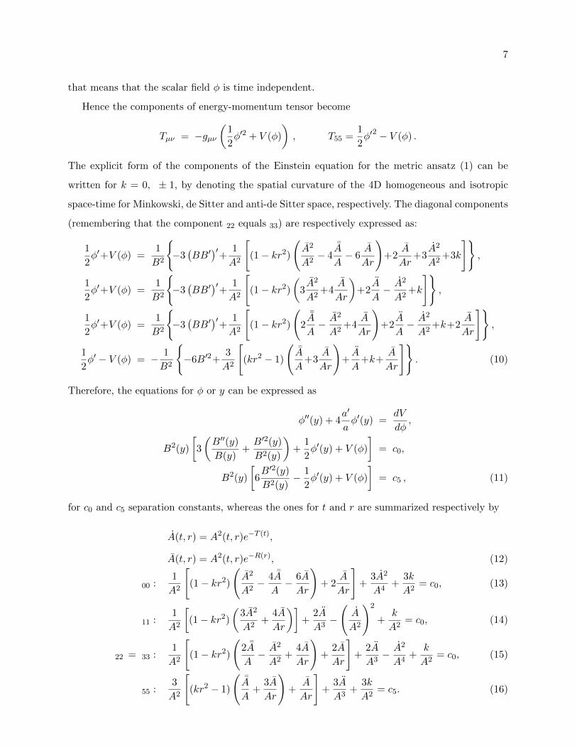
Centro de Matematica, Computacao e Cognicao,

Universidade Federal do ABC, 09210-580, Santo Andre, SP, Brazil and

International School for Advanced Studies (SISSA), Via Bonomea 265, 34136 Trieste, Italy.

(Dated: October 16, 2018)

Spherically symmetric time-dependent solutions for the 5D system of a scalar field canoni-

cally coupled to gravity are obtained and identified as an extension of recent results obtained

by Ahmed, Grzadkowskia and Wudkab [1]. The corresponding cosmology of models with reg-

ularized branes generated by such a 5D scalar field scenario is also investigated. It has been

shown that the anisotropic evolution of the warp factor and consequently the Hubble like

parameter are both driven by the radial coordinate on the brane, which leads to an emergent

thick brane-world scenario with spherically symmetric time dependent warp factor. Mean-

while, the separability of variables depending on fifth dimension, y, which is exhibited by the

equations of motion, allows one to recover the extra dimensional profiles obtained in Ref. [1],

namely the extra dimensional part of the scale (warp) factor and the scalar field dependence

on y. Therefore, our results are mainly concerned with the time dependence of a spherically

symmetric warp factor. Besides evincing possibilities for obtaining asymmetric stable brane-

world scenarios, the extra dimensional profiles here obtained can also be reduced to those

ones investigated in [1].

PACS numbers: 11.25.-w, 04.50.-h, 04.50.Gh

∗Electronic address: alexeb@ufscar.br†Electronic address: rogerio.cavalcanti@ufabc.edu.br‡Electronic address: roldao.rocha@ufabc.edu.br

arX

iv:1

411.

3552

v1 [

gr-q

c] 1

3 N

ov 2

014

2

Brane-world models are a straightforward 5D phenomenological realization of the Horava-

Witten supergravity solutions [2], where the hidden brane is placed at infinity and the moduli

effects from compact extra dimensions are neglected [3]. Once introduced in the context of an ef-

fective theory of supergravity on domain walls [4], brane-world scenarios are supported by seminal

results [5–8] which are relevant in realizing 4D gravity on a domain wall in 5D space-time [7–9].

Brane-world cosmology has also been investigated in several suitable contexts. Classes of exact

solutions with a constant 5D radius on a cosmologically evolving brane were provided in [10],

allowing unconventional cosmological equations with the matter content of the brane dominating

that of the bulk. This framework is in full compliance to standard cosmology, as the present values

of the Hubble parameter and of the cosmological background radiation temperature fits their

respective values at the time of nucleosynthesis. Moreover, brane-world cosmology in thin branes

has been studied for any equation of state describing the matter in the brane, where standard

cosmological evolution can be obtained after an early non-conventional phase in typical Randall-

Sundrum [11] scenarios, where the brane tension compensates the bulk cosmological constant. The

accelerated Universe could be the result of the gravitational leakage into extra dimensions on Hubble

distances rather than the consequence of non-zero cosmological constant [12]. Some attempts of

devising the Friedmann law on the brane have involved a dark radiation term due to the bulk

Weyl tensor, which depends linearly on the brane energy densities. For any equation of state on

the brane, the radiation was shown to evolve such as to generate conventional radiation-dominated

cosmology, consistent with nucleosynthesis [13].

Subsequent to the brane-world cosmology on thin branes, the thick brane-world paradigm has

exhibited a fine structure [1, 14, 15] that supports the above discussed phenomenology. In spite

of their success, thick brane-world models do encompass neither anisotropy on the brane nor the

important framework of asymmetric branes, as well as spherically symmetric thick brane worlds.

Even if anisotropic brane-worlds have been comprehensively investigated, there still are several

reasons to depart from the standard isotropic models, in particular focusing on spherically sym-

metric time-dependent warp factors, in the thick brane-world scenario. As an example, in Bianchi

I brane-world cosmology, for scalar fields with a large kinetic term, the initial expansion of the

Universe is quasi-isotropic. The Universe grows anisotropically during an intermediate transient

regime and the anisotropy finally disappears during the inflationary expansion [16]. In addition,

anisotropic brane-worlds are realized in the context of exact solutions of the gravitational field

equations in the generalized Randall-Sundrum model for an anisotropic brane with Bianchi type

I and V geometry, with perfect fluid and scalar fields as matter sources. Under the assumption

3

of a conformally flat bulk with vanishing Weyl tensor for a cosmological fluid obeying a linear

barotropic equation of state, the general solution of the field equations was expressed as an exact

parametric form for both Bianchi type I and V spacetimes [17]. The dynamics of the corresponding

anisotropy in such Bianchi type I and V cosmological scenarios has also been investigated in the

context of Randall-Sundrum brane-worlds [18], given that a Randall-Sundrum brane-world can be

mimicked without the assumption of spatial isotropy, by means of an homogeneous and anisotropic

Kasner type solution of the Einstein-AdS equations in the bulk [19]. Other interesting anisotropic

brane-world models have been studied in Refs. [20, 21].

On the other hand, observations of the CMB tell one that the Universe is isotropic with a

great accuracy [22]. The natural framework to approach this highly isotropic Universe implies

into assuming that the Universe setup from a highly anisotropic state, and thus a dynamical

mechanism gets rid of almost all its anisotropy. Inflation mechanisms [23, 24] are the most promising

candidates for explaining such a behavior. In these lines, the simplest generalization of FRW

cosmologies are the Bianchi cosmologies, as they provide anisotropic but homogeneous cosmologies,

where the central point of discussion is if the Universe can isotropize without additionally fine-

tuning the parameters of the model. The isotropization of Bianchi I brane-world cosmologies has

been investigated, from several points of view [25, 26]. It has been shown, for instance, that a

large initial anisotropy does not suppress inflation in a Bianchi I brane-world [16]. Otherwise,

considering negative values of dark radiation in Bianchi I models leads to interesting solutions for

which the Universe can both collapse or isotropize [18, 26, 27]. It is required that isotropization

should be accompanied by a phase of accelerated expansion in order to be a good candidate to

explain the results that indicate the current speeding up of the observable Universe [28]. This

latter observational fact is approached from two directions: modifying the gravitational sector [29]

or introducing dark energy [30]. From this point of view, a model in which a dark energy component

lives in a Bianchi brane-world combines both approaches.

The study of the dynamics of a scalar field with an arbitrary potential trapped in brane-world

model can be further performed [1, 15, 31, 32]. Homogeneous and anisotropic Bianchi I branes filled

also with a perfect fluid are the mostly approached models. In particular, by taking into account

the effect of a positive dark radiation term on the brane [34], the effect of the projection of the 5D

Weyl tensor onto the brane in the form of a negative dark radiation term is considered [33].

All the above-mentioned reasons motivate the investigation of both spherically symmetric and

anisotropic brane models. It is indeed worthwhile to emphasize that cosmological solutions of the

gravitational field equations in the generalized Randall-Sundrum model for an anisotropic brane

4

were obtained, with Bianchi I geometry and with perfect fluid as matter sources described by a

scalar field [35]. The solution admits an inflationary era and, at a later epoch, the anisotropy of the

Universe washes out. Two classes of cosmological scenarios are involved, regarding universes that

evolve from a singularity and without singularity [36]. Moreover, by using a metric-based formalism

to treat cosmological perturbations [37, 38], the connection between anisotropic stress on the brane

and brane bending are discussed in [39].

Our main aim here is to provide an initial approach for spherically symmetric thick brane

cosmology. By exploring the framework of isotropic thick branes [1, 14, 15], one can realize that

the separability of the warp factor is fundamental in order to explicitly describe the time-dependent

solutions. It is noway obvious that, for spherically symmetric thick brane-worlds, the warp factors

to be considered in this paper – that are dependent on time, extra dimension, and radial coordinate

on the brane – should be separable in the context of solving the equations of motion. Likewise, it

suggests that it might be hopeful to find time-dependent soliton solutions leading to non-separable

forms of the warp factor [40–42]. Separable solutions are normally discussed in the framework of

thin brane-world models that are rather unnatural in case of thick defects, since the brane thickness

∆ must fulfill the limits 2.0 × 10−19m . ∆ . 44µm [43], having thus a minimal thickness [44].

In fact, thick brane cosmology has been widely discussed in [40–42, 48], further regarding other

type of warp factors [49–53] and tachyonic solutions, with a decaying warp factor that enables

localization of 4D gravity as well as other matter fields [54]. Some applications in the thin brane

limit have been provided, e. g., in [45–47].

Departing from a general 5D spherically symmetric warped spacetime, our purpose is to solve the

coupled system of Einstein equations and the equations of motion for a scalar field. The procedure

introduced in the following results into an explicit formula for both the extra dimension-dependent

part of the warp factor and the spherically symmetric time-dependent component. The warp factors

for flat, closed, and open spacetimes are obtained and discussed, and the properties of Hubble type

parameter are also investigated. Our analysis results into deploying the fundamentals of thick brane-

world cosmology with time dependent spherically symmetric warp factors, exclusively departing

from the Einstein equations.

To provide a generalization of the successful achievements on brane-world cosmology in the thin

brane paradigm [10, 11] as well as in the thick brane scenario [1, 15], one considers 5D spacetimes

for which the metric assumes the following form:

ds2 = a2(t, r, y)gµνdxµdxν + dy2, (1)

5

where xµ denotes a chart of 4D coordinates on the brane, whereas gµν is the metric given by

gµνdxµdxν = −dt2 +

(dr2

1− kr2+ r2dΩ2

),

where dΩ2 stands for the usual area element of the 2-sphere and k denotes the curvature parameter

assuming the values −1, 0 and 1, leading respectively to an open, a flat or a closed Universe. The

function a(t, r, y) is the conformal scale factor extraordinarily depending upon the radial coordinate

r on the brane, also referred as a warp factor due to the extra dimension y in (1). The 4D solutions

are sourced by the bulk scalar field.

The action for scalar field in the presence of 5D gravity is given by

S =

∫d5x√−g

(−1

2gMN∇Mφ∇Nφ− V (φ) + 2M3

5R

), (2)

where g denotes the 5D metric, M5 is the Planck mass of the fundamental 5D theory and R denotes

the 5D Ricci scalar. For the above prescribed scenario, one assumes that the scalar field, φ, depends

exclusively on time and upon the extra coordinate, y, and V (φ) is the scalar field potential.

The Einstein equations and the equation of motion for φ resulting from the above action (2)

are provided by

∇2φ− dV

dφ= 0, (3)

RMN −1

2gMNR =

1

4M35

TMN , (4)

where ∇2 is the 5D Laplacian operator, and the energy-momentum tensor, TMN , for the scalar

field φ(t, y) reads

TMN = −gMN

(1

2(∇φ)2 + V (φ)

)+∇Mφ∇Nφ .

In particular, the energy-density (T00) is implied by φ(y) and localized near y = 0. Moreover, the

equation of motion for the scalar field is expressed by

φ′′ − 1

a2φ+

4a′

aφ′ − 2a

a3φ =

dV

dφ,

where one denotes ∂f∂t = f , ∂f

∂r = f , and ∂f∂y = f ′, for any scalar function f hereupon. By assuming

a static scalar field scenario, the components of the Einstein tensor are given by the following

6

expressions:

G00 = a2

3

[a2

a4−(a′′

a+a′2

a2

)+

k

a2

]+ (1− kr2)

[a2

a4− 2¯a

a3− 6a

a3r

]+

2a

a3r

,

G11 = −g11[

1

a2

(2a

a− a2

a2

)− 3

(a′′

a+a′2

a2

)+

k

a2

]− (1− kr2)

[3a2

a4+

4a

a3r

],

G22 = −g22[

1

a2

(2a

a− a2

a2

)− 3

(a′′

a+a′2

a2

)+

k

a2

]− (1− kr2)

[2¯a

a3− a2

a4+

4a

a3r

]+

2a

a3r

,

G33 = g33G22/g22,

G55 = 3

(2a′2

a2− a

a3− k

a2

)+ 3(1− kr2)

(¯a

a3+

3a

a3r

)− 3a

a3r,

G01 = 2

(2aa

a2−

˙a

a

),

G05 = 3

(aa′

a2− a′

a

),

G15 = 3

(aa′

a2− a′

a

).

The Einstein equations GMN = TMN , when 4M3∗ = 1, can be used to find the form of the warp

factor. By separating the variables a(t, r, y) = A(t, r)B(y), the Einstein equation G01 = T01 = 0

yields

0 = 2A

A−

˙A

A= ∂r lnA2 − ∂r ln A

⇒ lnA2

A= T (t)⇔ A = A2e−T , (5)

or

0 = 2A

A−

˙A

A= ∂t ln

A2

A

⇒ lnA2

A= R(r)⇔ A = A2e−R , (6)

implying that

A = AeR−T . (7)

The expressions A2 = A4e−2T and A2 = A4e−2R follow from (5), (6) and (7), and they imply that

˙A = = 2A3e−(T+R) ,

A = = A2e−T(

2Ae−T − T), (8)

¯A = A2e−R(2Ae−R − R

). (9)

One of the off-diagonal Einstein equations G05 = T05 = φφ′ yields

φφ′ = 3

(AB′

AB− AB′

AB

)= 0 ⇒ φ = 0 ,

7

that means that the scalar field φ is time independent.

Hence the components of energy-momentum tensor become

Tµν = −gµν(

1

2φ′2 + V (φ)

), T55 =

1

2φ′

2 − V (φ) .

The explicit form of the components of the Einstein equation for the metric ansatz (1) can be

written for k = 0, ± 1, by denoting the spatial curvature of the 4D homogeneous and isotropic

space-time for Minkowski, de Sitter and anti-de Sitter space, respectively. The diagonal components

(remembering that the component 22 equals 33) are respectively expressed as:

1

2φ′+V (φ) =

1

B2

−3(BB′

)′+

1

A2

[(1− kr2)

(A2

A2− 4

¯A

A− 6

A

Ar

)+2

A

Ar+3

A2

A2+3k

],

1

2φ′+V (φ) =

1

B2

−3(BB′

)′+

1

A2

[(1− kr2)

(3A2

A2+4

A

Ar

)+2

A

A− A2

A2+k

],

1

2φ′+V (φ) =

1

B2

−3(BB′

)′+

1

A2

[(1− kr2)

(2

¯A

A− A2

A2+4

A

Ar

)+2

A

A− A2

A2+k+2

A

Ar

],

1

2φ′ − V (φ) = − 1

B2

−6B′2+

3

A2

[(kr2 − 1)

(¯A

A+3

A

Ar

)+A

A+k+

A

Ar

]. (10)

Therefore, the equations for φ or y can be expressed as

φ′′(y) + 4a′

aφ′(y) =

dV

dφ,

B2(y)

[3

(B′′(y)

B(y)+B′2(y)

B2(y)

)+

1

2φ′(y) + V (φ)

]= c0,

B2(y)

[6B′2(y)

B2(y)− 1

2φ′(y) + V (φ)

]= c5 , (11)

for c0 and c5 separation constants, whereas the ones for t and r are summarized respectively by

A(t, r) = A2(t, r)e−T (t),

A(t, r) = A2(t, r)e−R(r), (12)

00 :1

A2

[(1− kr2)

(A2

A2− 4 ¯A

A− 6A

Ar

)+ 2

A

Ar

]+

3A2

A4+

3k

A2= c0, (13)

11 :1

A2

[(1− kr2)

(3A2

A2+

4A

Ar

)]+

2A

A3−

(A

A2

)2

+k

A2= c0, (14)

22 = 33 :1

A2

[(1− kr2)

(2 ¯A

A− A2

A2+

4A

Ar

)+

2A

Ar

]+

2A

A3− A2

A4+

k

A2= c0, (15)

55 :3

A2

[(kr2 − 1)

(¯A

A+

3A

Ar

)+

A

Ar

]+

3A

A3+

3k

A2= c5. (16)

8

The role of the bulk scalar field is to provide the cosmological constant on a brane as is clear from

Eqs.(12-15). By imposing c5 = Λ one has analogous cosmological implications for suitable limits,

where the warp factor has no dependence on r, as in the thick brane cosmology with isotropic warp

factor [1, 15]. In an isotropic thick brane-world the condition c5 = 2c0 = Λ holds [1]. Nevertheless,

in this scenario such two constants restrict further the form of the function A(r, t), when the above

equations are used, by the following relationship:

− 15

(kr2 − 1

c1r

)2

− 12(1− kr2)3/2

c1Ar2+ 6

√1− kr2c1Ar2

= 2c0 − c5 . (17)

Note that this consistency equation is trivial if the 4D scale factor is independent of the radial

coordinate, as in [1]. Now, by computing the difference of (14) and (15), one obtains the equation

(1− kr2)R− 1r = 0 which has solution

R(r) = lnc1r√

1− kr2, (18)

where c1 is a constant of integration. Moreover, the solution for Eq. (12) is provided by (hereon

one shall notice the index k in order to denote the dependence on k = 0,±1 in the following

expressions):

Ak(t, r) =c1

c1Yk(t) + fk(r), (19)

where Yk(t) is a constant of integration with respect to the r coordinate,

fk(r) ≡ ln

√1− kr2 + 1

r−√

1− kr2 , (20)

and Ak(t, r) depends on k = 0,±1. It implies hence that

Ak(t, r)

A2k(t, r)

= −Yk(t) = e−T (t) . (21)

We can simplify Einstein equations using (6), (8), (9), and (21) to make Eq.(13) — that corre-

sponds to the 00 component of the Einstein equations — to read:

Y 2k = −kY 2

k + wk(r)Yk + zk(r) , (22)

where wk(r) and zk(r) are respectively given by the following expressions:

wk(r) = −1

3

[2(1− kr2)e−R

(2R− 3

r

)+ 2

e−R

r+

6kfk(r)

c1

],

zk(r) = −1

3

(1− kr2)e−R

[−7e−R +

2fk(r)

c1

(2R− 3

r

)]+

2fk(r)

c1

e−R

r+ 3k

f2k (r)

c21− c0

.

9

The solutions for Minkowski, anti-de Sitter and de Sitter spacetimes are respectively provided

by:

Y ±−1(t) =1

4e±(t∓α−1)

[(e∓(t∓α−1) − w−1(r)

)2− 4z−1(r)

], (23)

Y ±0 (t) = α0 ±√z0(r)t, (24)

Y ±1 (t) =1

2

[w1(r)±

√w21(r) + 4z1(r) sin(t+ |α1|)

]. (25)

respectively for k = −1, 0, 1. The constant parameters α0, α±1 are constants of integration.

When fk(r) = 0, then Ak(t, r) = 1/Yk(t), and one has the results from [1] for thick brane

cosmology, with c5 = 2c0 = Λ, where Λ denotes the 4D cosmological constant. For the case

explicitly provided by Eq. (19), Ak(t, r) indeed does not depend on the r coordinate. Firstly, it is

evident that Ak(t, r) = 0 when r → ∞, as fk(r) diverges in this case. However, it is not properly

the useful case here. For k = 0, Ak(t, r) is independent of r when fk(r) = 0, namely, when r = 2/e.

Moreover, when k = 1, fk(r) = 0 for r = 1, and hence Ak(t, r) in Eq. (19) has no dependence on

the variable r. Finally, Ak(t, r) is merely a function of the cosmic time t for k = −1 when r solves

the algebraic equation√1+r2+1r = exp

(√1 + r2

), which is r0 ≈ 0.663.

Eqs. (23)-(25) lead to the solutions [1]

a(t) ∼

sech(t+ α−1) , k = −1 (Λ < 0)

1/(t+ α0) , k = 0 (Λ > 0)

sec(t+ α1) , k = +1 (Λ > 0)

(26)

For k = 0, 1 the metric is singular at a finite time t = −αa + (n+ 1/2)πk, (a = 0, 1), for n ∈ Z [1].

It further implies that in this particular case the Hubble parameter reads

H(t) =

tanh(t+ α−1) , k = −1 (Λ < 0)

1/(t+ α0) , k = 0 (Λ > 0)

tan(t+ α1) , k = +1 (Λ > 0)

(27)

for the appropriate limits above analyzed where fk(r) = 0.

Once the 00 component of the Einstein equations is considered, one can further analyze the 11

component. Eq. (14) thus reads

(1− kr2)e−R(

3e−R +4

c1rfk(r)

)+k

c1fk(r) + kY

+

[(1− kr2)e−R 4

r+

2k

c1fk(r)

]Y − 2

fk(r)

c1Y − 2Y Y + 3Y 2 = c0 .

10

It implies that

2Y

(Y +

fk(r)

c1

)= 3Y 2 + kY 2 + u(r)Y + v(r) , (28)

where uk(r) and vk(r) are respectively given by:

uk(r) =4

r(1− kr2)e−R +

2k

c1fk(r) ,

vk(r) = uk(r)fk(r)

c1+ 3(1− kr2)e−2R − k

c1fk(r)− c0 .

Moreover, the 22 and 33 components of Einstein equations are provided by Eq. (15), yielding

2Y

(Y +

fk(r)

c1

)= 3Y 2 + kY 2 +m(r)Y + n(r) , (29)

where

m(r) = e−R[−2(kr2 − 1)R+

6

r− 4kr

]+ 2k

fk(r)

c1,

n(r) = m(r)fk(r)

c1+ 3e−2R(1− kr2)− k

f2k (r)

c21− c0 .

Analogously, the 55 component of Einstein equations Eq. (16) reads

Y

(Y +

fk(r)

c1

)= 2Y 2 + kY 2 + g(r)Y + h(r) , (30)

where

g(r) = e−R[(kr2 − 1)

(3

r− R

)+ 1

]+ k

fk(r)

c1,

h(r) = g(r)fk(r)

c1− k

f2k (r)

c21− 2

(1− (kr2)2

c1r

)− c5

3.

Eqs. (28), (29) and (30) can be reduced to first order EDOs. By defining a new variable X = Y ,

Eqs. (28) and (29) can be written as

2XdX

dY(Y + α) = 3X2 + kY 2 + bY + c, (31)

where α = fk(r)/c1, for Eqs. (28) and (29), by identifying respectively b to u(r) and m(r), and c

to v(r) and n(r). Solutions are provided by

Y 2 = k1(Y + α)3 − kY 2 − 1

2bY − 1

3kα2 − 1

6αb− 1

3c, (32)

where k1 is a constant of integration. Note that when k1 = 0 the above equation has exactly the

same form of Eq. (22), thus has the same kind of solutions.

11

Moreover Eq. (29) can be recast analogously as

XdX

dY(Y + α) = 2X2 + kY 2 + g(r)Y + h(r) ,

and reduced to a first order EDO in a similar way, giving

Y 2 = k1(Y + α)4 − kY 2 − 2

3(αk + g(r))Y − 1

3(α2k + αg(r) + 3h(r)). (33)

In general, the above obtained equations do not exhibit analytical solutions. However when k1 = 0

the same form of the Eq. (22) is again achieved.

Given the form of the above equations, the constant parameter k1 fixes the initial acceleration

associated to the scale factor of the universe. One can compare it to the expected data for the

dynamics of the scale factor and set k1 according to the initial conditions.

In the set of Figs. 1-3 and Figs. 4-6 one respectively depicts the form for the warp factor Ak(t, r)

for k = 0,±1, and the associated Hubble like parameter, calculated from the respective warp factor.

12

1r

1

t

10

AHr,tL

FIG. 1: Graphic of the warp factor

A−1(t, r) in (19), for c1 = 2.

1r

1

t

-10

100

AHr,tL

FIG. 2: Graphic of the warp factor

A0(t, r) in (19), for c1 = 2.

1.1r

1

t

-10

30

AHr,tL

FIG. 3: Graphic of the warp factor

A1(t, r) in (19), for c1 = 2.

1r

1

t

-10

10

AHr,tL

FIG. 4: Graphic of the warp factor

A−1(t, r) in (19), for c1 = 0.1.

1r

1

t

-10

30

AHr,tL

FIG. 5: Graphic of the warp factor

A0(t, r) in (19), for c1 = 0.1.

1r

1

t

0

1

AHr,tL

FIG. 6: Graphic of the warp factor

A1(t, r) in (19), for c1 = 0.1.

The above two sets of plots indicate a dependence on the integration parameter c0, that is a

multiple of the brane cosmological constant in an isotropic thick brane-world. Instead, here the

13

constant c0 is related to the cosmological constant c5 = Λ by Eq. (17), and the spherical symmetry

of the warp factor sets in. This explains the dependence of the Ak(t, r) on the parameter c0.

When the constant of integration c1 in (17) is assumed to be equal to 2, Fig. 1 illustrates a

monotonically increasing scale factor both radially and temporally. The larger is the radial position

on the brane the steeper is the time dependence is. Fig. 2 presents a range of singularity that attains

lower values for the radial coordinate as time elapses. Fig. 3 illustrates a scale factor that increases

in the range presented therein. However such an increment is smoother as the cosmic time elapses.

When c1 = 0.1, Fig. 4 depicts a time-independent singularity for a fixed value r0 ≈ 0.663 for the

scale factor of a closed Universe, whereas the singularity evinced in Fig. 2 is smoother in Fig. 5.

Finally, Fig. 6 shows a similar profile as that one in Fig. 3, instead the radial increment is planer.

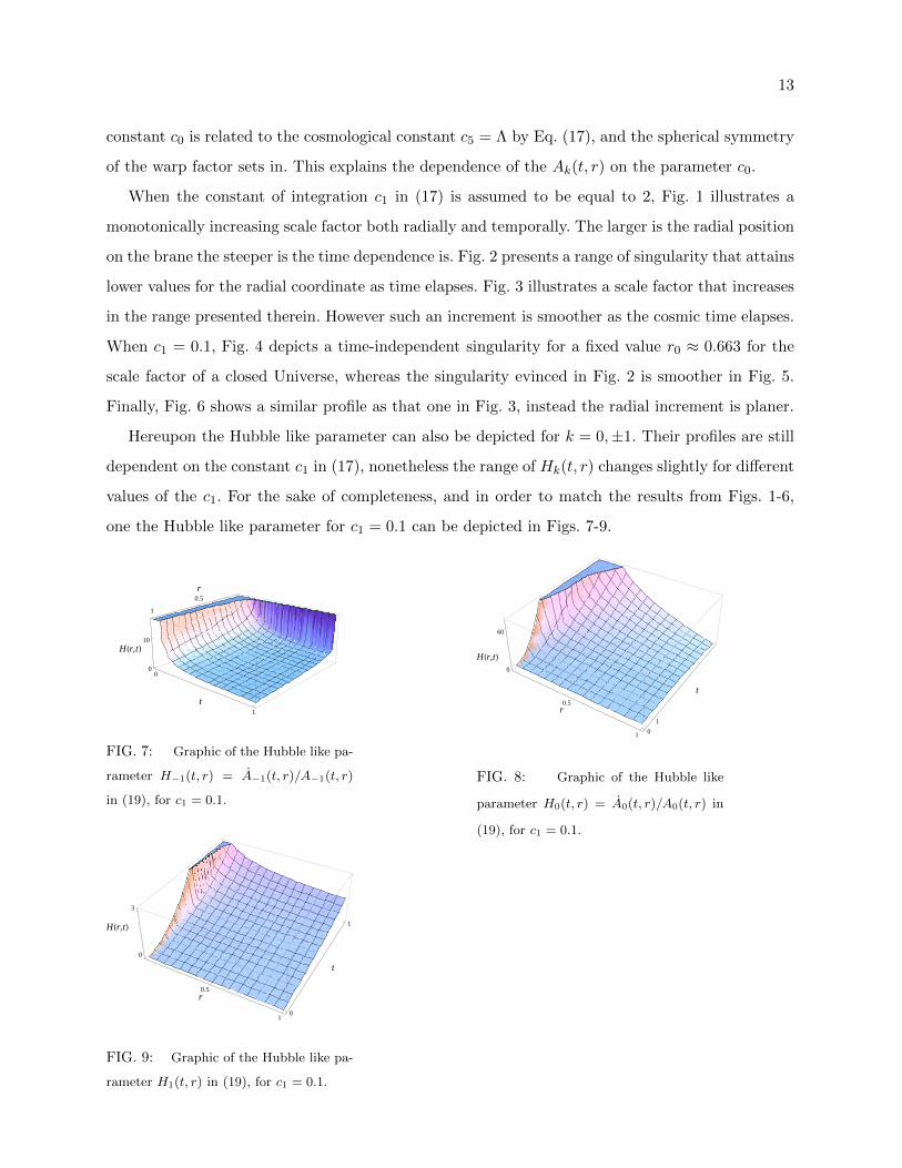
Hereupon the Hubble like parameter can also be depicted for k = 0,±1. Their profiles are still

dependent on the constant c1 in (17), nonetheless the range of Hk(t, r) changes slightly for different

values of the c1. For the sake of completeness, and in order to match the results from Figs. 1-6,

one the Hubble like parameter for c1 = 0.1 can be depicted in Figs. 7-9.

0.5

1

r

0

1

t

0

10

HHr,tL

FIG. 7: Graphic of the Hubble like pa-

rameter H−1(t, r) = A−1(t, r)/A−1(t, r)

in (19), for c1 = 0.1.

0.5

1

r

0

1

t

0

60

HHr,tL

FIG. 8: Graphic of the Hubble like

parameter H0(t, r) = A0(t, r)/A0(t, r) in

(19), for c1 = 0.1.

0.5

1

r

0

1

t

0

3

HHr,tL

FIG. 9: Graphic of the Hubble like pa-

rameter H1(t, r) in (19), for c1 = 0.1.

14

The above Hubble like parameters are led to the respective Hubble parameters (27), when the

suitable respective limits mentioned before Eq. (26) are taken into account. For the case k = 1,

the Hubble like parameter increases monotonically, being steepest for lower values of the radial

coordinate.

The y-dependent part of the solutions that are determined by Eqs. (10). By defining B(y) ≡

eb(y), it can be written as

3B′′ +3

2Λe−2b = −φ′2, (34)

6B′2 − 3Λe−2b =1

2φ′2 − V (φ), (35)

φ′′ + 4B′φ′ − dV

dφ= 0. (36)

As such equations are the same as those ones obtained in [1], our results for the extra-dimensional

profiles are likewise similar here. When one assumes a value for the function B(y), thus Eqs. (34)-

(36) determine φ(y) and V (φ), or vice-versa [55–58]. For instance, the warp factor B(y) =

ln[sinh(βy)] can be adopted in [1], for β usually assumed as a constant parameter, in order to

have A(y) ∝ e−|y| when y → +∞, recovering thus the Randall-Sundrum model. For small (large)

values of y, |y| . β−1 (|y| & β−1), the kink solutions are given respectively by

φsmall(y) = 2√

3 arctan[tanh(βy/2)],

φlarge(y) =

√−3Λ

2

1

βsinh(βy), (37)

These results can be turned into asymmetric thick brane-world scenarios, generated after adding

a constant to the superpotential associated to the scalar field. Asymmetric branes can be generated

irrespective of the potential being symmetric or asymmetric, and the sine-Gordon-type model in this

context can be shown to have a stable graviton zero mode, despite the presence of an asymmetric

volcano potential [59]. Indeed, the superpotential method described in [1] can be further extended

when one proposes the sine-Gordon-type model determined by the superpotential

Wc(φ) = 2

√3

2sin

(√3

2φ

)+ c,

that is obtained by the standard one, by shifting it by a constant parameter c such that |c| ≤√

6

[59]. The solutions for the equations

φ′ =1

2Wφ, (38)

A′ = −1

3W (φ), (39)

15

were obtained [59]:

φ(y) =

√3

2arcsin(tanh(y)), (40)

Ac(y) = − ln[sech(y)]− 1

3cy, (41)

where φ(y) is the standard solution of the sine-Gordon model, for c = 0. The Schrodinger like

equation with a quantum mechanical potential in conformal coordinates have already been studied

in [59] in order to derive an stable graviton asymmetric zero model 1. The asymmetry induced in

the thick brane-world scenario is also phenomenologically constrained to be consonant with the

AdS5 bulk curvature and with the experimental and theoretical limits of the brane thickness [44].

The constants c0 and c5 = Λ in (11) and (13)-(16) are severely constrained, besides Eq. (17), by

the fine tuning, relating the 4D and 5D cosmological constants, and the brane tension. To end up,

it is worthwhile to emphasize that for each k, the functions wk(r) and zk(r) in Eq.(22) constrain

the range of the variable r, and should be used to comply the model to observational data. The

same principle must be applied in the other differential equations for Yk(t). These constraints shall

be addressed in a forthcoming publication [60].

To finalize, further ways to analyze the system is to include the radial dependence in the bulk

scalar field that supports the radial dependence in the 4D scale factor. However, in this case, it is

no longer possible to solve the equations analytically.

Acknowledgements

A. E. B. would like to thank for the financial support from the Brazilian Agencies FAPESP

(grant 08/50671-0) and CNPq (grant 300809/2013-1) R. T. C. thanks to UFABC and CAPES for

financial support. R. da R. is grateful to SISSA for the hospitality, to CNPq grants No. 473326/2013-

2 and No. 303027/2012-6 and is also Bolsista da CAPES Proc. 10942/13-0.

[1] A. Ahmed, L. Dulny and B. Grzadkowski, Eur. Phys. J. C 74 (2014) 2862 [arXiv:1312.3577 [hep-th]].

[2] P. Horava, E. Witten, Nucl. Phys. B 460 (1996) 506 [arXiv:hep-th/9510209].

[3] R. Maartens, K. Koyama, Living Rev. Rel. 13 (2010) 5 [arXiv:1004.3962 [hep-th]].

[4] M. Cvetic, S. Griffies and S. Rey, Nucl. Phys. B 381 (1992) 301 [arXiv:hep-th/9201007].

1 Other models can be still studied in this context, as for instance the twisted solutions in [1], however it is out ofthe scope in the present paper.

16

[5] V. A. Rubakov, M.E. Shaposhnikov, Phys. Lett. B 125 (1983) 136.

[6] M. Visser, Phys. Lett. B 159 (1985) 22 [arXiv:hep-th/9910093].

[7] L. Randall, R. Sundrum, Phys. Rev. Lett. 83 (1999) 3370 [arXiv:hep-ph/9905221].

[8] L. Randall, R. Sundrum, Phys. Rev. Lett. 83 (1999) 4690 [arXiv:hep-th/9906064].

[9] M. Cvetic and H. H. Soleng, Phys. Rept. 282 (1997) 159 [arXiv:hep-th/9604090].

[10] P. Binetruy, C. Deffayet and D. Langlois, Nucl. Phys. B 565 (2000) 269 [arXiv:hep-th/9905012].

[11] P. Binetruy, C. Deffayet, U. Ellwanger and D. Langlois, Phys. Lett. B 477 (2000) 285 [arXiv:hep-th/9910219].

[12] C. Deffayet, G. R. Dvali and G. Gabadadze, Phys. Rev. D 65 (2002) 044023 [arXiv:astro-ph/0105068].

[13] J. Khoury and R. -J. Zhang, Phys. Rev. Lett. 89 (2002) 061302 [arXiv:hep-th/0203274].

[14] A. Ahmed and B. Grzadkowski, JHEP 1301 (2013) 177 [arXiv:1210.6708 [hep-th]].

[15] A. Ahmed, B. Grzadkowski and J. Wudka, JHEP 1404 (2014) 061 [arXiv:1312.3576 [hep-th]].

[16] R. Maartens, V. Sahni and T. D. Saini, Phys. Rev. D 63 (2001) 063509 [arXiv:gr-qc/0011105].

[17] C. -M. Chen, T. Harko and M. K. Mak, Phys. Rev. D 64 (2001) 044013 [arXiv:hep-th/0103240].

[18] A. Campos and C. F. Sopuerta, Phys. Rev. D 63 (2001) 104012 [arXiv:hep-th/0101060].

[19] M. G. Santos, F. Vernizzi and P. G. Ferreira, Phys. Rev. D 64 (2001) 063506 [arXiv:hep-ph/0103112].

[20] A. V. Frolov, Phys. Lett. B 514 (2001) 213 [arXiv:gr-qc/0102064].

[21] J. Ovalle, F. Linares, A. Pascua, R. Sotomayor, Class. Quantum Grav. 30 (2013) 175019 [arXiv:1304.5995

[gr-qc]].

[22] G. Hinshaw et al. (WMAP Collaboration), Astrophys. J. Suppl. 170 (2007) 288 [arXiv:astro-ph/0603451].

[23] A. H. Guth, Phys. Rev. D 23 (1981) 347.

[24] A. D. Linde, Phys. Lett. B 108 (1982) 389.

[25] G. Niz, A. Padilla, and H. K. Kunduri, JCAP 0804 (2008) 012 [arXiv:0801.3462].

[26] N. Goheer and P. K. Dunsby, Phys. Rev. D 67 (2003) 103513 [arXiv:gr-qc/0211020].

[27] A. Campos and C. F. Sopuerta, Phys.Rev. D 64 (2001) 104011 [arXiv:hep-th/0105100].

[28] A. G. Riess et al. (Supernova Search Team), Astron. J. 116 (1998) 1009 [arXiv:astro-ph/9805201].

[29] T. Clifton, P. G. Ferreira, A. Padilla, and C. Skordis, Phys. Rept. 513 (2012) 1 [arXiv:1106.2476].

[30] E. J. Copeland, M. Sami, and S. Tsujikawa, Int. J. Mod. Phys. D 15 (2006) 1753 [arXiv:hep-th/0603057].

[31] A. Wang, Phys. Rev. D 66 (2002) 024024 [arXiv:hep-th/0201051].

[32] S. Kobayashi, K. Koyama, and J. Soda, Phys. Rev. D 65 (2002) 064014 [arXiv:hep-th/0107025].

[33] D. Escobar, C. R. Fadragas, G. Leon, and Y. Leyva, Class. Quant. Grav. 29 (2012) 175006 [arXiv:1201.5672].

[34] D. Escobar, C. R. Fadragas, G. Leon and Y. Leyva, Astrophys. Space Sci. 349 (2014) 575 [arXiv:1301.2570

[gr-qc]].

[35] A. E. Bernardini and O. Bertolami, Ann. Phys. 338 (2013) 1 [arXiv:1212.0341 [gr-qc]].

[36] B. C. Paul, Phys. Rev. D 64 (2001) 124001 [arXiv:gr-qc/0107005].

[37] A. E. Bernardini and E. L. D. Perico, JCAP 01 (2011) 10 [arXiv:1012.4500 [astro-ph.CO]].

[38] A. E. Bernardini and E. L. D. Perico, JCAP 06 (2011) 001 [arXiv:1102.3996 [astro-ph.CO]].

[39] M. Dorca and C. van de Bruck, Nucl. Phys. B 605 (2001) 215 [arXiv:hep-th/0012116].

[40] M. Giovannini, Phys. Rev. D 76 (2007) 124017 [arXiv:0708.1830].

[41] D. P. George, M. Trodden, and R. R. Volkas, JHEP 0902 (2009) 035 [arXiv:0810.3746].

[42] A. Kadosh, A. Davidson, and E. Pallante, Phys. Rev. D 86 (2012) 124015 [arXiv:1202.5255].

17

[43] D. J. Kapner, T. S. Cook, E. G. Adelberger, J. H. Gundlach, B. R. Heckel, C. D. Hoyle and H. E. Swanson,

Phys. Rev. Lett. 98 (2007) 021101 [arXiv:hep-ph/0611184].

[44] J. M. Hoff da Silva and R. da Rocha, Europhys. Lett. 100 (2012) 11001 [arXiv:1209.0989 [hep-th]].

[45] R. da Rocha and J. M. Hoff da Silva, Phys. Rev. D 85 (2012) 046009 [arXiv:1202.1256 [gr-qc]].

[46] C. H. Coimbra-Araujo, R. da Rocha and I. T. Pedron, Int. J. Mod. Phys. D 14 (2005) 1883 [astro-ph/0505132].

[47] J. M. Hoff da Silva and R. da Rocha, Phys. Rev. D 81 (2010) 024021 [arXiv:0912.5186 [hep-th]].

[48] G. German, A. Herrera–Aguilar, D. Malagon-Morejon, I. Quiros and R. da Rocha, Phys. Rev. D 89 (2014)

026004 [arXiv:1301.6444 [hep-th]].

[49] M. Gogberashvili, A. Herrera-Aguilar, D. Malagon-Morejon, R. R. Mora-Luna and U. Nucamendi, Phys. Rev.

D 87 (2013) 084059 [arXiv:1201.4569 [hep-th]].

[50] M. Gogberashvili, A. Herrera-Aguilar, D. Malagon-Morejon and R. R. Mora-Luna, Phys. Lett. B 725 (2013)

208 [arXiv:1202.1608 [hep-th]].

[51] M. Carrillo-Gonzalez, G. German, A. Herrera-Aguilar and D. Malagn-Morejn, Gen. Rel. Grav. 46 (2014) 1657

[arXiv:1210.0597 [hep-th]].

[52] W. T. Cruz, A. R. Gomes and C. A. S. Almeida, Europhys. Lett. 96 (2011) 31001 [arXiv:1110.3104 [hep-th]].

[53] A. E. Bernardini and O. Bertolami, Phys. Lett. B 726 (2013) 512 [arXiv:1304.4138 [hep-th]].

[54] G. German, A. Herrera-Aguilar, D. Malagon-Morejon, R. R. Mora-Luna and R. da Rocha, JCAP 02 (2013)

035 [arXiv:1210.0721 [hep-th]].

[55] O. DeWolfe, D. Freedman, S. Gubser, and A. Karch, Phys. Rev. D 62 (2000) 046008, [arXiv:hep-th/9909134].

[56] M. Gremm, Phys. Rev. D 62 (2000) 044017 [arXiv:hep-th/0002040].

[57] V. Afonso, D. Bazeia, and L. Losano, Phys. Lett. B 634 (2006) 526 [arXiv:hep-th/0601069].

[58] D. Bazeia, L. Losano, R. Menezes and R. da Rocha, Eur. Phys. J. C 73 (2013) 2499 [arXiv:1210.5473

[hep-th]].

[59] D. Bazeia, R. Menezes and R. da Rocha, Adv. High Energy Phys. 2014 (2014) 276729 [arXiv:1312.3864

[hep-th]].

[60] A. E. Bernardini, R. Cavalcanti, and R. da Rocha, Observational Aspects of Thick Anisotropic Brane Cosmology,

in preparation.