A COMPARISON OF THE FINITE DIFFERENCE AND FINITE ELEMENT METHODS FOR HEAT TRANSFER CALCULATIONS*

A. F. EMERY H. R. MORTAZAVI

UNIVERSITY OF WASHINGTON SEATTLE, WASHINGTON

INTRODUCTION

Of the many approximate or numerical methods used to solve heat transfer problems, the finite difference and finite element approaches have become the mosF: widely known and used. The finite difference method (FDM) is the older, being introduced in 1928111, and until recently, probably the better known and more extensively used for both research and production studies. The finite element method (FEM) is newer121 and has not been used for heat transfer studies to a comparable degree, although it is the dominant method for structural analyses.

Because the FEM has a short history of use for heat transfer, there is considerable confusion about the relative values of the two methods and under which conditions one method is to be preferred. Both methods are based upon minimizing the weighted error in satisfying the first law of thermodynamics. Two common FDM's are: the heat balance FDM (BFDM) [31, based upon minimizing, over a nodal volume with unit weight; the mathematical FDM (MFDM) [4,51, based upon collocating at discrete points, usually regularly spaced upon coordinate lines. The FEM is based on the Galerkin method [63 in which the error is minimized over an elemental volume with a weight function equal to the temperature.

The purpose of this paper is to compare the two methods by describing their bases and their application to some common heat transfer problems. It will be no surprise that neither method is clearly superior or that, In many instances, the-choice is quite arbitrary and depends more upon the codes avail- able and upon the personal preference of the analyst than upon any well defined advantages of one method.

ANALYTICAL PROCEDURES

The numerical solution of a heat transfer problem by either FDM or FEM, is usually done in the following steps as shown in table 1:

*This work was supported by NASA grant NAG-l-41

51

https://ntrs.nasa.gov/search.jsp?R=19820015603 2018-06-04T14:07:12+00:00Z

TABLE 1 ORDER OF ANALYSES

1. Subdivision of the region into nodes or elements 2. Definition of material properties, initial temperatures and boundary

conditions 3. Evaluation of the thermal conductance between nodes and the

capacitance of each node 4. Formation of the global conductance and capacitance matrices 5. Imposition of the boundary conditions 6. Solution for the nodal point temperatures and heat fluxes 7. Display of the results

Both methods tend to use these same steps, although the division between the steps may be more or less clearly defined depending upon the method used and upon the organization of the computer code.

A. The Mesh

The process of subdividing the region into elements or nodal volumes, commonly called 'meshing', is usually accomplished by a separate program. Although the FDM mesh was generally created by hand, the FEM programs relied, almost from their inception, upon numerical mesh generators. This difference in approach was probably due to:

1. FDMs usually utilize nodal points which are oriented along coordinate lines. Thus irregular regions are difficult to model automatically and use is often made of hand meshing with special imaginary nodal points. If the region is susceptible to treatment by a different coordinate system, the mathematical problem is usually recast. For example, elliptical or oblique coordinate systems are often used.

2. FEM codes were first used in structural problems where an organized nodal point mesh was clearly evident and an arbitrary mesh could not be used (e.g., the frame and stringer structures of aircraftL71). By the time the FEM was applied to continuum problems, it had been observed that the solution of the Laplacian gave rise to an acceptable mesh. Because the FEM could be applied to such a wide range of geometries and because the number of elements tended to increase quickly, a need for automatic mesh generation became obvious. As a consequence an emphasis was placed upon automatic mesh generation for the FEM.

Several symposia[8] have been organized soley to discuss sophisticated methods for the FEM and for the FDM used in computational fluid dynamics. Unfortunately, few of the thermal FDM use other than the simplest mesh generators. Lately we find that most codes, whether FDM or FEM tend to use the same mesh generators. Since this mesh generation is also used to identify the regions occupied by the different materials, to define intial temperatures, as well as to prescribe the boundary conditions, the entire mesh generation process is usually referred to as 'PRE-PROCESSING'.

52

B. Thermal Conductance

The primary difference between the FDM and the FEM lies in the methods used to construct the thermal conductance between the nodes.

1. FDM

In the FDM, the conductance is formed in one of two ways. The simplest approach is illustrated in figure 1 and is based upon the heat balance equation

I pc$dv= /q,da+ /

q'dv (1) v A v

where the energy conducted through the surface is approximated by the linear relationship

%(i,j> = qij = kij Aij 'Tj -Ti) le. . iJ (2)

The quantity Ai./l.. is a geometric value which, in two dimensions, th2 addles of the triangle formed from the nodes[91.

can be related to Equivalently it can be found as illustrated in figure 1 by constructing the area Aij which is perpendicular to the line joining the nodes and located at the mid point of the line. Although this method is difficult to implement, it can be done automatically and also provides a technique for determining the set of closest nodes which surround a node. Unless the nodes are regularly spaced, in which case the BFDM becomes the MFDM, the BFDM is of low accuracy, O( Ax ).

The second method, the mathematical FUM (MFDM), is based upon expressing the differential equation

by finite differences using a variety of different numerical approximations to achieve a desired level of accuracy. The method consists of establishing an interpolating function in space, usually a polynomial, and performing the needed differentiation. Another method is to express Tj in terms of Ti,through a Taylor series expansion. By combining the expressions for the temperatures at different nodal points, i.e., establishing different stencils, figure 2, it is possible to achieve a very high order of accuracy. For example the 5 point stencil is accurate to O(Ax2), while the 9 point is of O(&t4). However, the 13 point is accurate not only to O(Ax4 ) but ensures that V4T as well as V2T=0 is satisfied[lOl.

For a non-linear problem it is usual to express & %j$ as [ I

3 k aT ax I 1 Xax =

k,zx+$g (4)

and to evaluate each term separately. Unfortunately this approach does .not give a conservative set of equations (in P. D. Lax's sense) and energy is not conserved in steady state problems. As a consequence, the non-linear FDM is usually confined to the 5 point stencil for regular regions and the heat balance method for irregular regions.

53

2. FEM

The finite element method is based upon the Galerkin approach in which a stationary value of the integral

I = s$[% [g)' + kY [g)2 - PC g2 + 2qNT] dv + pnTda (5)

v A is sought[lll. For steady state problems, the Galerkin and the variational approaches are equivalent and the method, in conjunction with the dual formulation (i.e., the adjoint problem), can be used to establish bounds upon the solution. For transient problems, there is no variational formulation and no bounds can be found.

The procedure consists of approximating the temperature within the element by T

T(x,y) = L=l

nl(x,y)ae = <II> {a) (6)

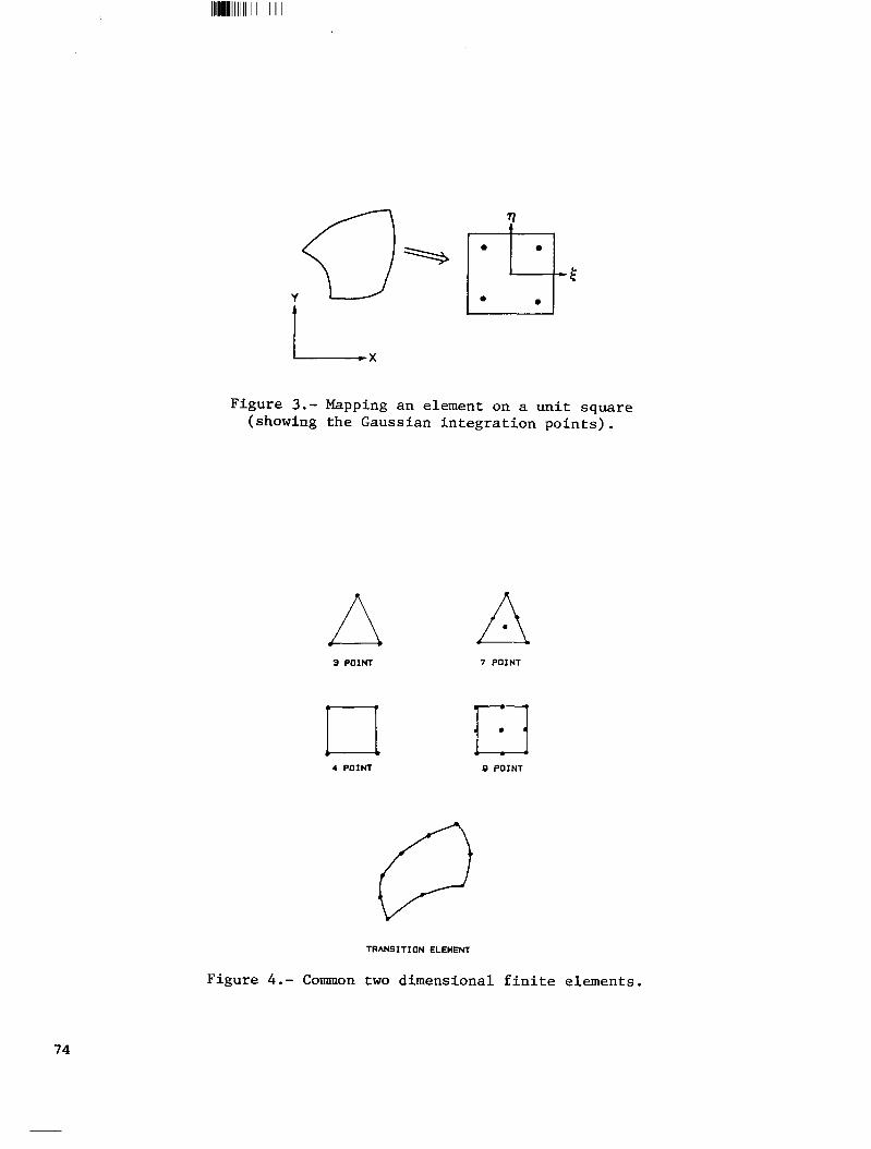
where the interpolating functions, n(x,y) can be chosen at will to satisfy any desired criteria, subject only to the restriction that there be a sufficient number of nodes in the element to determine the coefficients, al . Since each element is treated as an entity, it is common to map the element into a simpler shape to expedite the integration, figure 3. Consider that a local set of coordinates, 5 , r), are defined and that the mapping

J (7)

is used where the number of terms J need not equal the number OF terms I used in the temperature interpolation. We then have

{T^) = [AlCal , T(x,Y) = <n> [A]-%} = <N> (T^} (W

(2) = [B]Cb) x= <ii> [ES]-'{;;} = <fi>{;;) (8b)

Thus for one element the conduction term is of the form

(9d

(9b)

and

(10)

where J is the Jacobian of the mapping.

54

Although it is obvious that the spatial interpolation function, i , must ensure compatability of elements (i.e., that an edge common to two elements must be the same when viewed from either element) it is not necessary that the temperatures be compatible. In structural mechanics FEM, incompatible formulations are sometimes used, but almost all thermal problems use compatible temperature functions. When the same number of functions are used to express the mapping and the temperature, the element is termed 'iso-parametric'. Although the isoparametric element is the usual, subparametric elements are often used for heat source problems or when an unusual temperature distribution is desired.

The most common 2-D elements are the 3 and 6 node triangles and the 4 and 8 node quadrilaterals, figure 4. Much of the research in the FEM has been devoted to developing new interpolating functions (i.e., new elements) and identifying their characteristics, particularly with respect to the numerical integration required.

3. Differences

Probably the most striking difference between the FDM and the FEM is the usual lack of continuity of the heat flux in the FEM. Each element is treated separately and if only compatibility of temperature is imposed, the heat flux at the edge common to two elements is not continuous. By contrast, the FDM has a continuous heat flux. Although the effect of lack of continuity of the heat flux is usually not important, it can show up in the form of an oscillating temperature profile where an overshoot in one node is compensated for by an undershoot at a neighboring node in order to minimize the integral over the entire region.

c. Capacitance Matrix :

In the FDM, the capacity term, PC aT/ at is represented by the simple lumped term

(PiciVil aTi at (11)

where Vi is the volume surrounding the node i. In the FEM, the use of the interpolating function gives rise to the consistent capacitance matrix

(12) C L C nl""' nn 1

in which the storage at each node is related to that at every other node in the element. This difference in the two capacitance matrices is responsible for much of the difference in the solutions to transient problems and is discussed further in the EXAMPLE section. For 3 node triangular elements with regular node spacing, the FDEI and FEM have identical conductance and capacitance matrices. Other FEM elements give different matrices, usually as indicated by the sign of the off-diagonal terms. In the FEM the integration is usually accomplished through Gaussian integration and the need to evaluate the properties and the Jacobian at each point contributes to the longer execution times of the FEM.

55

D. Assemblage of the Global Matrix

1. FDM

In the FUM, each node is treated in turn, and the conductances are entered into the global matrix as they are determined. The process is simple and straightforward and requires very little computer time. Unless a.n FEM preprocessor mesh is used, FDM codes generally make use of a separate matrix which identifies the nodes which interact, the corresponding value of the term Aiad~f~J;~f tz;km;;;:iaL numbers to permit rapid determination of the average

2. FEM

In the FEM, the element matrix is first evaluated, then assembled into the global matrix. If the global matrix cannot be stored in core, it is necessary to search through the elements to treat only those containing the nodes whose equations are currently in core. This assembly process tends to be reasonably time consuming and may contribute to the reduced speed of the FEM.

3. Comparison

Table 2 lists some typical execution times for FDM and FEM solutions. In general, the FEM assembly costs rise quickly as the number of nodes per element is increased. Figure 5[121 shows some comparable results for a structural problem and the extra expense of the assembling is easily seen. (The figure also shows that for some variables the FDM is superior while for others the FEM is. Because of this, it is difficult to define one method as being the best for all parameters of a problem.)

n

3 5 7 9

13 17 19 31 33 61 65

TABLE 2 RELATIVE EXECUTION TIMES FOR THE TRANSIENT PROBLEM

Equal Time Step Sizes

FDM FEM L-W Explicit C-N Linear Quadratic Cubic Special

Cubic .8 1 1 1.8

1.4 1.5 2 5.4 6.5 4.4 5.5

3.7 3.5 6 32 36 24 36

17 12 24 218 249 183 125 540

107 64 117 1624 1880 1500 4350

760 407 1230 12200 14700 n = number of elements L-W = Lax Wendroff

C-N = Crank Nicolson

56

E. Boundary Conditions and Irregular Meshes

Although the greatest fundamental difference between the FDM and the FEM lies in the formulation of the conductances and capacitances, the greatest practical difference lies in their treatment of boundary conditions and irregularly shaped regions.

1. FDM

Specified temperature nodes are treated by ignoring the equation for the node. Boundary flux conditions are difficult to treat for irregular meshes unless one uses the simple heat balance formulation (BFDM) with its low order of accuracy. Irregular meshes have been studied for years with emphasis on using triangular surface elements[l31. Since many analysts tend to define their nodes along coordinate lines, it is most common to make use of imaginary nodes, figure 6, special differencing equations to achieve the desired accuracytl41, arbitrary grids[l5], or even no nodes, but only cellstl61. In general, the advanced mesh generators used in fluid computations and the automatic high order boundary gradient differencing methods are not used in production FD methods. Consequently they suffer from reduced accuracy at irregular boundaries. On the other hand, research FDM's almost always maintain high accuracy at all types of boundaries.

2. FEM

Irregular regions are handled in the same manner as any other region. The accuracy is limited only by the ability of the mesh generator to represent the boundaries. This ability is probably the greatest strength of the FEM.

Specified temperature nodes are handled in two ways. In the first, the equation is deleted from the matrix and the right hand sides of all affected equations are modified. Another way is to replace the diagonal coefficient by a very large number, L, and the right hand side by L*T[17]. Although faster and simpler than the first method, the accuracy of the computer may limit the effectiveness of this approach.

Prescribed heat flux boundary conditions are handled better by FDM than by FEM. Because in the FEM each element is treated separately, the accuracy is limited by the interpolating accuracy of the element shape functions. By contrast, the FDM analyst can easily modify a difference equation to achieve the desired accuracy. The FEM analyst must call for a boundary element which is different from the interior element, figure 4, and may have some difficulty in merging this higher order element with the rest of the mesh unless a special mesh generator or slide lines are used.

F. Solving the Equations - Steady State Problems

Although sparse matrix solvers have become popular recently[l8], most FDM and FEM codes use some form of elimination (usually Gauss or Cholesky) and rely upon a banded matrix or sky line approach to achieve fast solution times[l91. For highly non-linear problems, iterative solutions may be used, especially by FDM codes.

57

1. J?DM

E'DM codes normally use direct reduction or iteration. Because of the way in which the global matrix is assembled, iteration is a common procedure and, when used, the global matrix is not created. If reduction is used, only enough equations to treat the band are kept in core and they are shifted immediately after each nodal equation is reduced (the wave front method). Although iteration is an appropriate technique, convergence is difficult to determine and because iterative acceleration factors are often unknown, many users are reluctant to employ iterative techniques. Fortunately most heat transfer problems can be treated by using the SOR method and values of the over relaxation factor can be quickly approximated. For problems which are not symmetric or do not have Young's property AC201, the SSOR techniqueL211 is easy to implement and convergence is very rapid. Non-linear problems are ideally suited to the iterative method and rarely increase the solution time by an appreciable amount. Considerable research is still being conducted into improving the rate of convergence and treating highly non-linear problems[221.

2. E'EM

Most FEM codes use a reduction process with a subsequent back substitution. Even with a skyline procedure, care should be taken to minimize the band width. To do this, most FEM codes will use a band width minimizimg program after the mesh generation1231, although this may complicate the identification of the nodal point positions within the code. Non-linear problems are treated in two ways:

1. The matrices are reformed and solved for each iteration.

,(n),(n) = ,h>

2. A residual is found, and an increment, AT determined from

IS1 (Id = {R) (n)- [K] {T} (n-1) AT(“) = [K]-‘{e)(“)

(134

(13b)

It is common to use a mixture of these two methods by applying the boundary loads in increments, calculating a new K for each increment, but iterating within the increment using a constant K until the residual is sufficiently smallL241. Method 1 requires excessive computer time and may not converge. Method 2 requires that the original conductance matrix be stored in order to calculate the residual. Either method is expensive, and for highly non-linear problems, the iterative FDM appears to be preferred. Suendermann [251 suggests that the ratio of the execution times for hydrodynamic problems is 100 to 27b2/2+18b for implicit methods and 100 to 23bi for explicit methods where b=band width and 1 the number of FEM iterations.

In both methods it is often desireable to know the amount of heat added to a constant temperature node. In the F'DM, the calculation of QiiS simply done by calculating the conductances and evaluating the heat balance. In the FEM, this may be done by using the original K matrix if it is stored. A simpler way

58

is to permit a specified temperature node, Ti to float by connecting it to a constant temperature, T, , through a very high conductance, KH , and evaluating

Qi = 'k CT&> (14) Although much simpler, the size of KH required may be so large that some

computers may not accurately calculate the correct inverse of the global conductance matrix. In this case the energy balance will have to be computed for the node under question.

G. Solving the Equations - Transient Problems

In general, both the FDM and the FEM simply step along in time, re-evaluating K and C at each time step, if needed. If the time steps are large or the problem is highly non-linear, then iterations may be needed within each time step [261. If the non-linearities may be expressed analytically a Runge-Kutta technique may be applied to the resulting non-linear equations[271. For very non-linear problems, Gear's method may be used [281. Regardless of why the matrices must be re-evaluated (i.e., changing boundary conditions or non-linear properties) Young's method 1291 can be used to modify the matrix and the solution with a minimum increase in time, although the code structure may have to be changed considerably.

H. Graphical Display

Besides printed output, the most common output is a spatial plot of a single variable or contour plots. Such plots oE the temperature are relatively easy to generate for either the FDM or the FEM if a mesh generator was used. If the FDM was based upon the heat balance approach, then it is necessary to create a set of minimum size triangular elements to perform the contour plotting [301, especially if contour smoothing is to be used [31]. Table 3 illustrates the times necessary to compute a set of triangular elements connecting 418 nodes. If the region is complete, the element calculation is rapid. If there is one or more internal voids, then the establishment of the mesh may be very expensive, as indicated by the third table entry.

TABLE 3 Contour Plotting Times

1. Temperature contours 5.6 seconds 2. Temperature contours-establishing a mesh 30 seconds 3. Temperature contours-establishing a mesh

with an internal void 120 seconds

If the contours are to be based upon other than linear interpolation or if the heat fluxes between elements are to be plotted, the FEM is much simpler to use since the element interpolation functions may be used, both to give a higher order curve fit and to interpolate to establish the values of qx and qy at the nodal points.

59

In general the FEM output is much better suited than the FDM output to graphical display, particularly for curved surfaces. To permit rapid detection of input errors and for rapid analyis, both a plane and an isometric (with hidden line capability) contour plotter should be available.

EXAMPLES

We present some typical examples of the use of the two methods.

A. Distributed Heat Sources

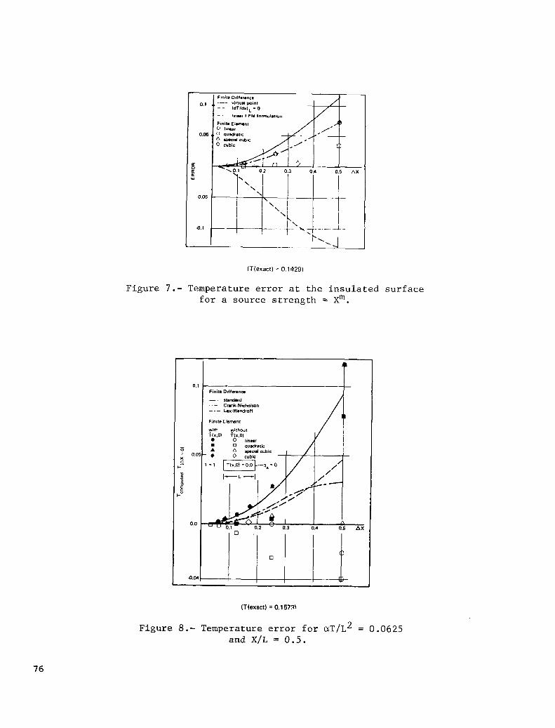
Consider a one dimensional problem, _ _ o<xc 1, with a distributed source strength of q'=xm ., The problem was treated with an FDM using two different boundary conditions and the FEM source term and the FEM utilizing 4 different elements[32]. Figure 7 illustrates the error in the temperature at the insulated surface. The solid line is for both the MFDM with a virtual point

and for the BFDM. The dashed line is for the MFDM using the zero heat flux boundary condition and shows the underprediction of the temperature because of the lack of a source at the last node. The FEM results are substantially better for two reasons. Firstly, the source is not lumped at a single node, but is distributed between nodes, thus permitting a better representation of the spatially varying heat source (this is clearly shown by the equivalence of the results for the FDM using the FEM source term and the FEM.) Secondly, the higher accuracy of the FEM temperature interpolation permits consideration of temperature variations higher than the linear. The special cubic element of Tocher[331 provides for continuity of the temperature and the heat flux at the interface between elements. Over a range of source functions, O<m<5, this special cubic was not found to be any better than the quadratic or the normal cubic element, neither of which ensure continuity of the heat flux.

B. Transient Temperatures - 1-D

Consider the one-dimensional slab with an insulated back surface and a front surface whose temperature is suddenly reduced to zero. Figure 8 illustrates the results obtained using several FD methods and several FEM elements[32]. In the FEM we write,

T(x,y,t) = < N(x,y) ' {i(t)) (15)

Tn+l = Tn + [&+'+(l-a)+"]at

FK + &]r;pl = (I-a)[C]{$jn + c Lt] {t>" + CX{R)~+' -

or

p + &] mnfl = [- (1-a)K + & {?jn + CX{R)~+' + (l-a){# ]

(16)

(17)

60

One may also use a combined space-time interpolant 1341

T(x,y,t) = 1 Ni(x,y,d i (18)

but this method does not yet appear to be in regular use for producton codes. $n figure 8, the use of equation 16 with T(x,O)=O is referred to as 'without T'. If T(x,O) $0 or if equation 17 is used, the solution is referred to as 'with T'. The relatively poor FEM results are due to the use of the consistent capacitance matrix and the impulsive start. Figure 9 compares the FEM with consistent matrices and the FDM with the lumped capacitance[35]. Because the FEM overpredicts the eigenvalues (i.e., yields an overly stiff system) while the FDM underpredicts,. the FEM results show an early time overshoot. This can be corrected by lumping the capacitance 'terms [36,37] or by expressing f by using a different basis which is orthogonal to the shape functions for T[38,39]. The effect of lumping is shown most clearly by examining the element eigenvalues for the 8 node quadrilateral as illustrated in figure 10. Lumping may also be effected by using a reduced order of integration, which softens the transient response, but care must be taken to avoid creating singular capacitance matrices[40]. The best results have been found when using the same order of integration as for the conductance. For non-linear problems, a one point integration has been found to be sucessful[41]. Lumping has the further advantage of simplifying the algorithm and reducing the execution time and has been extensively used for structural problems[42]. Figure 11 shows the error in the effective thermal diffusivity for several different methods. Cubic Hermite elements[43] are seen to be the best, in agreement with the results of figure 8.

Another solution is to permit the discontinuous change to take place over several time increments, a technique commonly used in hydrodynamic shock analyses. Figure 12 shows that while this smooths the results, it does not reduce the lag in the response which is due to the excessive dissipation of the FDM and lumped FEM solutions. A better way is to evaluate the right hand side at the half time intervals or by a consistent time interpolation[44]. As illustrated, this gives the best performance. Table 2 lists the execution times needed for the different methods for an equal number of time steps. For non-linear prob'lems in which the matrices must be reformed and re-solved, the FEM is substantially slower than the FDM, particularly when the SSOR method is used.

C. Singular Problems - Standard Methods [32]

Consider a two-dimensional plate as shown in figure 13. Because of the sharp edge of the insulated splitter plate, the heat flux at the tip is infinite and of the form

q = Klfl(8)/& + K2f2(8)& (19)

This problem was treated by using the MFDM and the FEM.

61

II II

1. FDM

Figure 13 illustrates the results obtained with different mesh sizes using a 5 point stencil. Substantial errors in the temperature and in the heat fluxes, figure 14, were found and even a reduction from Ax=Ay=l/4 to Ax=1/20 did not yield convergence, even for mesh points further than 2Ax from the singularity.

2. FEM

Figures 13 and 14 also show the comparable results found by using different elements and sizes. Of the three elements used, the quadratic is seen to give the best results. Table 4 lists the execution times. Although the quadraticelement times are long,the times necessary to produce an accuracy in the temperature comparable.to that of the linear element or the MFDM are approximately equal. On the other hand, the accuracy in evaluating the heat flux is much better than that of the FDM, with the result that the comparable execution times are much less.

TABLE 4 RELATIVE EXECUTION TIMES FOR THE SINGULAR PROBLEM 2:l RECTANGULAR NODAL GRID, STANDARD PROGRAMMING

number of Ax(=Ay) nodes

FEM linear quadratic cubic

FDM SOR SSOR

15 l/4 1 1 0.8 1.1 45 l/8 3.6 10.4 110 4.5 3 66 l/10 6.0 8.1 4.3

153 l/16 20.5 121 3097 21 20 231 l/20 39.1 274 53 31 361 l/32 172 1531 207 183

D. Singular Problems - Lagrangian Variables

As described above, problems with concentrated heat sources or with singular heat fluxes can rarely be treated with standard FDM or FEM programs since the interpolating functions are incapable of adequately representing the singular temperature field. In both methods, the interpolating functions can be expanded to include the singular behavior. If the strength of the singularity is known, the extra term simply serves as an additional heat source. If the strength is unknown, the FDM and FEM must be modified. For the mM, let OT be the FD approximation to the field equation and BT be the FD approximation to the boundary condition. Then by expressing the temperature as

T = T(smooth> + KlS

we find

62

OT Z v2T + K,(oS - V2S) I

BT f BT + K1(BS - BS)

It is thus apparent that the effect of the singularities can be considered by adding the pseudo heat source and boundary heat fluxes.

For the FEM, the appropriate formulation is1451:

T = < n > {;3 + Kl(S-<N> {s^3) (21)

In this solution the value of Kl is considered to be a Lagrangian variable which is determined by differentiating the integral to yield extra equations of the form:

$$3= bd{T^> + Kl(S,-<N,> {s^)){N,)

aI= (S aKl

,-<N,> {s^>) <N,> {T^3 + (S,-<N,“‘3)2K1

(224

(22b)

Figure 13 illustrates a problem in which the magnitude of the singularity is unknown. In the FDM, the value of Kl is found by applying the field equation to the closest boundary points, in addition to using the expanded boundary conditions. When using the FEM, it is not necessary that all elements contain the singular terms, only those near the singularity. However it has been found important1461 that a smooth transition between the singular elements and the regular elements be provided by establishing transition elements in which the temperature is of the form

T(x,y) = <N&j + f(x,y) Kl (S-<N>(z)) (23)

in which the function f(x,y) has the value of 1 along edges common with the singular elements and 0 along edges common with the regular mesh. As seen from figure 15, relatively coarse meshes for both the FHM and the FEM are sufficient to determine q,with good accuracy if the singular term is included, but even increasing the number of elements by a factor of 16 is insufficient if it is omitted.

Table 5 gives a comparison of the values of the temperature at point P as determined by several different FDM and FEM solutions and the equivalence of the two singular methods is apparent. Table 6 lists the values of the singular strengths, Kl and K2 . Although K2 varies considerably, KI (which is the dominant singularity) is quite constant. If K2 were to be computed more exactly, then it would be necessary to include the next term in the singular series[47]. The superiority of the singular approach is evident.

63

Ax

l/2 l/4 l/6 l/8 l/10 l/12 l/16 l/20. l/24 l/32

TABLE 5 COMPARISON OF Tp BY DIFFERENT METHODS (Figure 13)

FEM FDM 1st order 2nd order 1st order Singular 1st order 2nd order Singular

triangle triangle quadrilateral 0.1429 0.1176 0.170 0.1591 0.1737 0.1579 0.083. 0.133 0.1659 0.1771 0.1674 0.1697 0.1784 0.1717 0.181 0.151 0.174 0.1815 0.1721 0.1741 0.1738 0.1756 I 0.166 0.178 0.1824 0.1759 0.1775 0.173 0.180 0.1827 0.1772 0.176 0.181 0.1827 0.1781 0.1793

Ax

l/2 l/4

l/8

number of singular elements

2(all) 2 6 8(all) 2 6

12 18 32(all)

TABLE 6 SINGULARITY STRENGTHS AND T-

FEM

K1 K2

1.285 0.091 0.170 1.276 0.067 0.179 1.234 -0.032 0.179 1.224 -0.045 0.178 1.275 -0.056 0.182 1.1325 -0.492 0.1815 1.232 -0.048 0.182. 1.212 -0.077 0.181 1.203 .-0.086 0.181 1.195 -0.094 0.181

FDM T

P iY K2 'p

Under some conditions, the analytical form of the singular terms may be so complex that the integration required for the FEM may be difficult to perform with acceptable accuracy. In this case, the singular FDM, which satisfies only at the nodal points, is a more useful method.

One of the interesting features of the FEM is that it is often possible to distort an element to produce the desired singularity[481. Referring the the splitter plate problem, if an 8 node quadrilateral is used and the mid side nodes are shifted to the quarter points as indicated in figure 16, the element automatically includes a square root singularity. The figure compares these quarter point element results with those of the singular FDM and the comparison is excellent.

64

E. Radiation Problems

Regions with internal voids which have strongly radiating boundaries pose a problem, particularly for the FEM, even if the boundary conditions are linearized, since all of the nodes interact simultaneously and the resultant band width is very large and portions of the matrix are dense. One approach is to consider the problem as two problems, the radiation problem, and the conduction problem. The radiation problem is solved separately,ensuring radiative equilibrium among the nodes. The ,radiative heat flux is then considered as a known heat flux and applied to the right hand side of equation 5. Because the boundary condition is so non-linear, it often proves necessary to use a strong under-relaxation factor to limit the flux change to assure convergence and avoid the overshoot observed with impulsively changed boundary conditions as indicated by the transient problem. If the rest of the problem is linear, this approach is satisfactory. If the rest of the problem is highly non-linear, an iterative FDM appears to work more efficiently.

F. Phase Changes

Probably the most difficult problem to treat effectively by either method is that of a transient phase change. Three methods, figure 17, appear to be the most common. In the first, the interface motion is computed on the basis of the conservation equations, just as is done for fluid shock calculations[491. If an implicit time s.olution is used, this method requires the solution of non-linear algebraic equatons[50,51]. The second method is to assume that the phase change occurs over a small temperature range, T. The latent heat is then approximated by a large specific heat value, or the enthalpy may be used as the primary dependent variable. An iterative solution is often needed to ensure that the interface is maintained at the correct fusion temperature and special care must be taken in evaluating the capacity[51,52]. In a third method, based upon the use of the enthalpy and the temperature, the interface position is not explicitly determined. In this method an artificiaL specific heat is not used. This method has not been fully developed and some problems have been noted if the enthalpy interpolatation is other than a step function[531. In its present form, this method may be better suited for use with the BFDM.

Figure 18 compares some typical results of the first two methods using FDM and FEM. Comini's solution[51] used Lee's time integration and gave slightly greater solidification depths than the other methods. The FDM interface was slightly in error at the earliest time because of the lumped capacitance, although it quickly gave correct values. The FDM enthalpy solution gave essentially identical results.

65

G. Conclusions

Having used both FDM and FEM for more than 2 decades to solve a variety of thermal problems, ranging from simple I-D transient cases to 3-D singular biological problems, we have drawn the following general conclusions.

1. The mathematical FDM appears to be best suited to research problems, especially ones for which the analyst wishes to ensure that the boundary conditions are treated with high order accurate schemes or ones in which special algorithms are used at specified nodal points.

2. The heat balance FDM appears to be best for: 1. Highly non-linear problems, for which iterative solutions are

efficient. 2. Problems in which the continuity of the heat flux is important. 3. Multi-dimensional problems involving change of phase.

3. The FEM is best suited to: 1. Irregular regions for which the automatic mesh generation and a

library of highly accurate elements permit good modelling of the region and the consequent temperature profile.

2. Mildly non-linear problems for which the iterations are few. 3. Problems for which graphical output is important. 4. Problems in which special temperature profiles are desired, since

these may be easily obtained with special elements. 5. Problems involving singular temperature fields or concentrated

heat sources. 6. Problems in which different approximations are to be used in

different regions or problems which involve the joining of several parts.

Although each method may appear to be best for a particular class of problems, we have also reached the rather general conclusions that:

1. The analyst should be knowledgeable about both methods, at least to the extent that their general characteristics are understood.

2. Because thermal FEM elements are still being developed, their characteristics are not generally known. The analyst should experiment with such elements until their behavior, singly or in concert with other elements, is clearly understood[54]. In particular, the performance of any one element is not intuitively obvious and may not be representative of a 'similar element' for another problem[SSl.

3. Except for very special problems, either approach is satisfactory and which method used depends more upon the availability and familiarity of codes (and pre- and post-processors) than upon any intrinsic differences between the two methods.

66

We recognize that this last conclusion is rather fuzzy, but since the results obtained with either method will vary as the stencil or the element is changed, we have found that nothing will compensate for the analyst's insight into the detailed characteristics of the method used. Since such insight is normally developed only by exercising a program on a variety of problems and since it is rare that any one person is comfortably familiar with more than one method, it is not surprising that there is a considerable tendency to continue using a familiar code, even if some shortcomings exist.

A recent round robin test of FDM and FEM[561 applied to a typical mixed boundary condition, transient problem (fig. 19) showed that either method was satisfactory and that the apparent value of either depended more upon the pre- and post-processors available than upon the intrinsic characteristics or accuracies of the methods. On the other hand, for some conditions, particularly anisotropic problems, the results of reference 57 indicate that the FDM may be more accurate, but when there was no cross coupling, the FEM was superior.

Readers should consult references 58 and 59 for more information about the FDM and references 60 and 61 for detailed insight into the FEM. Current work. in the FDM is concentrated on improving the accuracy and execution times, with special emphasis on thermal network correction methodst621. Extensions of the FEM to treat combined convection-conduction problems and to merge the thermal FEM with the structural FEM, taking the different mesh requirements and time responses into consideration, are also being studied1631. In addition, some recent work[64,651 has shown that elliptical PDE's and conduction-convection problems can be accurately solved by combining collocation at the Gaussian points with the FEM elements. Finally, we should note that the development of small-scale personal computers, which are slow but may be dedicated to specific tasks, can be expected to have profound influences upon the structure of the computer codes, the use of interactive execution, and the specific algorithms used[661. In this context, it should be recognized that the substructuring method, which is commonly used on these small computers, cannot be used for transient problems.

67

NOMENCLATURE

A B C C f I 3 k K 1 n N 4' 'n

4,

Qi R S t T

tt

r ci B

&I

1 P.

0

Area FDM boundary condition operator Specific heat capacity Capacitance matrix Transition function Integral Jacobian of transformation Thermal conductivity Thermal conductance matrix Distance between nodes Interpolating function Shape function Generated heat density Boundary heat flux

Directional heat flux

Net heat input to a node

Right hand vector Singular function Time Temperature

Time derivative of temperature

Smooth temperature distribution Weighting parameter Boundary condition operator Error Coordinates of unit square Density Change Nodal values Approximation to the Laplacian

68

REFERENCES

1. Courant,R., Friedricks,K. and Lewy,H., "On the Partial

2.

3.

4.

5.

6.

7.

8.

9.

10.

11.

12.

Difference Equations of Mathematical Physics", Math. Annalen., DD%?-74 a 1928 ii sser,lj., "A Finite Element Method for the Determination of Non-Stationary Temperature Distributions and Thermal Deformations", Proc. Conf. Matrix Meth. Struct. Mech., USAF Inst. of Tech., Wright-Patterson AFB, pp925-943, 1965 Fox,L., Numerical Solution of Ordinary and Partial, Differential Equations, Pergamon Press, Oxford, 1962 Forsythe,G.E., and Wasow, N.R., Finite Difference Methods for Partial Differential Equations, J. Wiley, N.Y., 1960 Babuska,I., Prager,M. and Vitasek,E., Numerical Processes in Differential Equations, J. Wiley, N.Y., 1966 Leipholz,H., Direct Variational Methods and Eigenvalue Problems in Engineering, Noordhoff Publ., Netherlands, 1977 Turner,M.J., Clough,R.W., Martin,H.C., and Topp,L.J., "Stiffness and Deflection Analysis of Complex Structures", J.Aero. Sci., ~~805-823, 1956 Smith,R.E., Numerical Grid Generation Techniques, NASA Conf. Publ. 2166, 1980 Dusinberre,G.M., Numerical Analysis of Heat Flow, McGraw-Hill, N.Y., 1949 Bickley, W.G., "Finite Difference Formulas for the Square Lattice" , Q. J. Mech. Appl. Math., ~~35-42, 1948 Strang,G. and Fim., An Analysis of the Finite Element Method, Prentice Hall,~N.J., 1973 Bushnell,D., "Finite Difference Energy Models versus Finite Element Models: Two Variational Approaches in One Computer Program", Numr. and Corn& Meth. Struct. Mech., (Fenves,S. J. ,et al , eds) Asiflress, N;~~p~~6, 1973

13.

14.

15.

Hildebrand,F.B., Finite Difference Equations and Simulation, Prentice Hall, N.J., 1968 Lau,P.C.M., "Finite Difference Approximationsfor Ordinary Derivatives" ,,,Intl. -J. Num. Meth..Engng., ~~663-668, 198i Jensen,P.S., Solution ofwo-Dimensional Boundary Value

16.

17.

18.

19.

20.

Problems by-Arbitrary Grid Finite Difference Methods", Adv. ;;;;is;;;:.JPDEr, (Vichnevetsky,R., ed), AICA, ~~80-85, 1975

(Morris,J.i.:' Cell Discretization", Conf. Appl Num. Anal.,

ed) Springer-Verlag, Berlin, 1971 -- Payne,N.A.and Irons,B., ref in Zienkiewics,O.C., The Finite Element Method, 1st ed., McGraw Hill, N.Y., 1967 Eisenstat,S.C., Schultz,M.H. and Sherman,A.H., "Efficient Implementation of Sparse Symmetric Gaussian Elimination", Adv. Comp. Meth. PDE., (Vichnevetsky,R., ed) AICA, ~~33-45, 1975 Irons,B.M. and Kan, D.K.Y., "Equation Solving Algorithms for the Finite Element Method", Num. Comp. Meth. Struct. Mech., (Fenves,S.J., et al, eds.) Academic Press, N.Y., pp497-511, 1973 Young,D.M., Iterative Solutions of Large Linear Systems, Academic Press, N.Y., 1971

69

21. Sheldon,J.W., "On the Numerical Solution of Elliptical Difference Equations", Math. Tables, pplOl-111, 1955

22. Zedan,M. and Schneider,G.E., "3-D Modified Strongly Implicit Procedure for Finite Difference Heat Conduction Modelling", paper AIAA-81-1136, AIAA 16th Thermophysics Conf., Palo Alto, Calif, 1981

23. Schauer,D.A., "A Finite Element Bandwidth Minimizer"' Lawrence Livermore Lab., Livermore, Calif., 1973

24. Hogge,M.A., "Secant versus Tangent Methods in Non-Linear Heat Transfer Analysis", Int. 3. Num. Meth. Engng., ~~51-64, 1980

25. Suendermann,J., "Thexlicam ofnite Elements and Finite Difference Techniques in Hydrodynamical Numerical Models", Formulation and Computational Algorithms in FEM,US-German Symp., (Bathe,K-J., et al, eds) MIT Press, Ma, 1977

26. Chung,B.T.F. and Chang,T.Y., "Heat Transfer in Solids with Variable Thermal Properties and Orthotropic Conductivity", paper AIAA-81-1137, AIAA 16th Thermophysics Conf., Palo Alto, Calif., 1981

27. Aguirre-Ramirez,G. and Oden,J.T., "Finite Element Technique Applied to Heat Conduction in Solids with Temperature Dependent Thermal Conductivity", Int. J. Num. Meth. Engng., ----- pp345-355, 1973

28. Franke,R. and Salinas,D., "An Efficient Method for Solving Stiff Transient Field Problems Arising From FEM Formulations", Comp. Math. with Appl., ~~15-21, 1980

29. Young,R.C., "Efficient Nonlinear Analysis by Factored Matrix Modification", paper M4/3, Fourth SMiRT Conf., San Francisco, Calif, 1977

30. Patterson,M.R., "CONTUR- A Subroutine to Draw Contour Lines for Randomly Located Data", ORNL/CSD/TM-59, 1978

31. Emery.A.F., "PLOT- A General Purpose Plotting Program with Smoothing", Mech. Engng. Dept, Univ. of Washington, Seattle, Wash., 1980

32. Emery,A.F. and Carson,W.W., "An Evaluation of the Use of the Finite Element Method in The Computation of Temperature", ASME 3. Heat Trans., ~~136-145, 1971

33. Echer,J.L. and Hartz,B.J., "Higher Order Finite Element for Plane Stress", ASCE J. Engng. Mech., pp149-172, 1967

34. Chung,K.S., "Thxuxh-Dimensmoncept in the Finite Element Analysis of Transient Heat Transfer Problems", Int. J. Num. Meth. Engng., ~~315-325, 1981

35. Emery,A.F., Sugihara,K. and Jones,A.T., "A Comparison of Some of the Thermal Characteristics of Finite Element and Finite Difference Calculations of Transient Problems", Num. Heat -- Trans., pp97-113, 1979

36. Schreyer,H.L. and Fedock ,J.J., "Orthogonal Base Functions and Consistent Diagonal Mass Matrices for Two Dimensional Elements", Int. J. Num. Meth. Engng., pp1379-1398, 1979

37. Tong.P, PiasHx.and marelli,L.L., "Mode Shapes and Frequencies by Finite Element Methods Using Consistent and Lumped Masses", Comp. and Struct., ~~623-638, 1971

70

38. Hinton,E., Rock,T. and Zienkiewicz,O.C., "A Note on Mass Lumoinq and Related Processes in the Finite Element Method".

3g. 'F",F'hlt~~Bk~n'd"~~~~u~~~.~~~u~t~ Dynamics, pp245-249, 1976 a Finite E ement Mass Matrix Lumpins

by Numerical Integration-with no Convergence Rate Loss", && 3. Solids Struct., ~~461-466, 1975

40. xckson,C.P., "Singular Capacity Matrices Produced by Low Order Gaussian Integration in the Finite Element Method", Int. 3. Num. Meth. Engng., ~871-877, 1981

41. Huebner,K.~., The Finite Element Method for Engineers, J. Wiley, N.Y., 1975

42. Key,S.W., Beisinger,Z.E., and Krieg,R.D., “HONDO-II, A Finite Element Computer Program for the Large Deformation Dynamic Response of Axisymmetric Solids", Sand 78-0422, Sandia Laboratories, Albuquerque, N.M, 1978

43. Vichnevetsky,R. and De Schutter,F., "A Frequency Analysis of Finite Difference and Finite Element Methods for Initial Value Problems" , Adv. Comp. Meth. for m, (Vichnevetsky,R., ed) AICA. ~~46-52. 1975 P -

44. Bett&cburt,J:M., Zienkiewicz,O.C. and Cantin,G., "Consistent Use of Finite Elements in Time and the Performance of Various Recurrence Schemes for the Heat Diffusion Equation". Int. J. --. Nun. Meth. Engng., pp931-938, 1981

45. Tii5FY.A.F.. "The Use of Sinsularitv Proqramminq in Finite

-

Difference-and Finite Element Computation of Temperature". ASME J. Heat Trans., ~~344-351, 1973

46. Benz1GiS.E. and Beisinqer.Z.E.. "CHILES- A Finite Element Computer Program that Calculates the Intensities of Linear Elastic Singularities", SLA-73-0894, Sandia Laboratories, Albuquerque, N.M., 1973

47. Emery,A.F. and Segedin,C.S., "Singularity Programming- A Numerical Technique for Determining the Effect of Sinqularities in Finite Difference Solutions- Illustrated by Application to Plane Elastic Problems", Int. J. Num. Meth. - Engng., ~~367-380, 1972

48. Emerv.A.F.. Neishb0rs.P.K.. K0bavashi.A.S. and L0ve.W.J.. "Stress Intensity Factors in Ed&-Cracked Plates Subjected to Transient Thermal Singularities", ASME J. Press. Vess. Tech., DDlOO-105. 1977

49. Mbrretti,G., "Floating Shock Fitting Techniques for Embedded Shocks in Unsteady Multi Dimensional Flows", Proc. 1974 HTFMI, Stanford Univ. Press, ~~184-201, 1974

50. Fisher,I. and Medland,I.C., "The Multi Dimensional Stefan Problem: A Finite Element Approach", Finite Element Meth. in Wm., Univ. N.S. Wales, Australia, ~~767-783, 1974

51. Comini,G. Del Guidice,S., Lewis,R.W. and Zienkiewicz,O.C., "Finite Element Solution of Non-Linear Heat Conduction Problems with Special Reference to Phase Change", Int. J. Num. ----- Meth. Engng., ~~613-624, 1974

71

I I II IIIII III I I

52. Labdon,M.B. and Guceri,S. Ii, "Heat Transfer of Phase Change Materials in Two Dimensional Cylindrical Coordinates", paper AIAA-81-1046, AIAA 16th Thermophysics Conf., Palo Alto, Calif., 1981

53. Ronel,J. and Baliga,B.R., "A Finite Element Method for Unsteady Heat Conduction with or without Phase Change" ASME paper 79-WA/HT-54, ASME Winter Annual Mtg., N.Y., 1979

54. Robinson,J., "Element Evaluation- A Set of Assessment Points and Standard Tests", FEM in the Commercial Environment, (Robinson,J., ed) Robinson and Assoc., England, ~~218-241, 1978

55. Haggenmacher,G.W. and Lahey,R.S., "Practical Aspects of the Finite Element Method", FEM in the Commercial Environment, (Robinson,R., ed). Robinson and Assoc., England, pp70-102,1978'

56. Emery.A.F., Workshop on FE and FD Methods, Sandia Laboratories, Livermore, Calif., 1979

57. Sen Gupta,S.K. and Akin,J.E., "A Numerical Study of Coefficient Modelling", Adv. Comp. Meth. for m, (Vichnevetsky,R., ed) AICA, pp285-2m9K

58. Mitchel1,A.R. and Griffiths,D.F., The Finite Difference Method in Partial Differential Equations, J. Wiley, N.Y., 1980

59. Smith,G.D., Numerical Solution of Partial Differential Equations: Finite Difference Method, Oxford Univ. Press, Oxford, 1978

60. Strang,G., "Variational Crimes in the Finite Element Method", Math. Found. of the FEM with Appl. to PDE, (Aziz,A.K., ed) Academic Press, N.Y., pp689-710, 1972

61. Mitchel1,A.R. and Wait,R., The Finite Element Method in Partial Differential Equations, J. Wiley, N.Y., 1977

62. Shimoji,S., "A Comparison of Thermal Network Correction Methods", paper AIAA-81-1139, AIAA 16th Thermophysics Conf., Palo Alto, Calif., 1981

63. Thornton,E.A. and Wieting,A.R., "Integrated Transient Thermal-Structural Finite Element Analysis" AIAA/ASEM/ASCE/AHS 22nd Struct. Structural Dynamics and Materials Conf., Atlanta, Ga., 1981

64. Houstis,E.N., Lynch,R.E., Papatheodorou,T.S. and Rice,J.R., "Development Evaluation and Selection of Methods for Elliptical Partial Differential Equations", Adv. Comp. Meth. PDE., (Vichnevetsky,R., ed) AICA, ~~1-6, 1975

65. Herbst.B.M.. "Collocation Methods and the Solution of Conduciion-Convection Problems", Int. J. Num. Meth. Engng., ---~ DD1093-1101. 1981

66. &rensen,MI: "A Case Study Based on TOPAS",FEM in the Commercial Environment, (Robinson,J.,ed) Robinson and Assoc, England, ~~1-5, 1978

72

Figure l.- Finite difference mesh for the heat balance method.

+-I- S-POINT

. . ISPOINT

g-POINT

7-POINT

13POINT SKEWED

Figure 2.- Finite difference nodal point arrangements.

73

lllllllllllllllllllllll I I I II I

Figure 3.- Mapping an element on a unit square (showing the Gaussian integration points).

A 3 POINT

4 POINT

A . 7 POINT

TRANSITION ELEMENT

CII . S POINT

Figure 4.- Common two dimensional finite elements.

74

DISPLACEMENT

0 o 6 I6 24

-20 0 50 100

NUMBER OF MESH POINTS

- FEM --- FDM

Figure 5.- Error (%) and computer time (set) for a clamped shell using an FEM and an FDM [12].

IMAGINARY

FINITE DIFFERENCE

FINITE ELEMENT

Figure 6.- Treatment of irregular boundaries.

75

lT(exact) = 0.19291

Figure 7.- Temperature error at the insulated surface for a source strength = Xm.

(Tkxact) = 0.157~1

Figure 8.- Temperature error for aT/L2 = 0.0625 and X/L = 0.5.

76

wt 2 /f

Figure 9.- Temperature at the insulated surface using an FDM and an FEM with 2 node linear (L-2) and 3 node linear (L-3) elements.

CONSISTENT MATRIX

12

??= 5.33 8 L”MPECf4YATRlX

8

25.1

7.2

Figure lO.- Eigenvectors for the eight node element showing the effect of lumping.

77

-.-- 7 6 5

1 L~n.ar FEH 2 Ouadrotlo FEM 3 Ouodrot(o B-SPlsnr 4 Cublo H.rmlt. FEM 5 Storm.,--Num.ror 6 5 Point FIIH 7 3 Point FDH

Figure ll.- Error in the numerical diffusivity for different methods [43].

50-

I 3 %40- k-5

I 0 IO

..... ..“- ANALYTICAL - TDOT, R=O --- TDOT, R= 1 ----- TOLD x 50 - - LUMPED, FDM

I I I 20 30 40 50

TIME

Figyre 12.- Transient temperature response for a slab using TWO) = 0 with ramps of 0 and 1 At and a consistent method using a modified initial surface temperature (TOLD = 50).

78

Figure 13.- Temperature at point P for the singular problem.

lqx -. 1.560)

Figure 14.- Heat flux at point Q for the singular problem.

79

Figure

Figure 15.- Values of the heat flux along the insulating splitter plate.

L-sirlgularity programing

+ l/4 point element

I 1 0 1D 21)

TIME- ET/W2

16.- Calculation of the time dependent singularity strength for the problem of figure 13.

TEMPERATURE

INTERFACE

Figure 17.- Enthalpy and interface models for phase change calculations.

IO

E 0.8

w cl

5 0.6

F 4 ” ‘, 04

* 0.2

0

-ANALYTICAL A FDM - INTERFACE 0 COMINI - ENTHALPY 0 FISHER - ENTHALPY + FISHER - INTERFACE

1 ~~ 1 I I I 0 0.2 0.4 0.6 0.8 IO

Figure 18.- Solidification front position for a plane problem.

81

FINITE DIFFERENCE

Figure 19.- Comparison of FDM and FEM results for a mixed boundary condition problem.

82