L O A N COPY: RETURN TO qFWL TECHNICAL LIBRARY

KIRTLAND AFB, N. M.

THERMAL CONDUCTANCE OF A N D HEAT GENERATION IN TIRE-PAVEMENT INTERFACE A N D EFFECT ON AIRCRAFT BRAKING

C. David Miller

Lewis Res,earch Center Cleveland, Ohio 44135

N A T I O N A L A E R O N A U T I C S A N D SPACE A D M I N I S T R A T I O N W A S H I N G T O N , [E. C. J A N U A R Y 1976 BI

TECH LIBRARY KAFB, NM

I11111111111111llul1111Il111111111Ill11 - -. . .I 1. Report No. I 2. Government Accession No.

. - .--. -

EFFECT ON AIRCRAFT BRAKING 6. Performing Organization Code

~- -_- _. 7. Author(s) 8. Performing Organiza,tion Report No.

C. David Miller E-8357 -­

10. Work Unit No.~ ~~~

9. Performing Organization Name and Address 505-08 Aerospace Safety Research and Data Institute 11. Contract or Grant No. Lewis Research Center

I Cleveland, Ohio 44135 -. ~

13. Type of Report and Period Covered 12. Sponsoring Agency Name and Address Technical Note

National Aeronautics and Space Administration 1 14. Sponsoring Agency CodeI Washington, D. C. 20546 - _ . I

15 Supplementary Notes

. - - ~­16. Abstract

A finite-difference analysis w a s performed on temperature r eco rds obtained from a f r e e rolling automotive t i re and from pavement surface. A high thermal contact conductance between t i re and asphalt w a s found on a s ta t is t ical basis, probably about 3x10 4 W/(m2)(K) or grea te r . Aver age sl ip due to squirming between t i re and asphalt was about 1. 5 mm. Consequent friction heat w a s estimated as 64 percent of total power absorbed by bias-ply, belted t i re . Extrapolation of resu l t s to a i rc raf t t i r e indicates potential braking improvement by even moderate increase of heat absorbing capacity of runway surface.

.I. .~ ..- __17. Key Words (Suggested by Author ls) ) 18. Distribution Statement

Heat conduction; Tires; Friction; Contact Unclassified - unlimited conductance; Braking; Aircraft runway; Road STAR Category 05 (rev. ) resis tance

. . . -

THERMAL CONDUCTANCE OF AND HEAT GENERATION IN TIRE-PAVEMENT

INTERFACE AND EFFECT ON AIRCRAFT BRAKING

by C. David Mi l le r

Aerospace Safety Research and Data Institute Lewis Research Center

SUMMARY

A finite-difference analysis w a s conducted on data provided by the University of Michigan, which was obtained during research conducted under an NASA grant. The data consisted of temperatures recorded by (1) thermocouples embedded within the tread of a free-rolling automotive t i re and (2) nickel-grid resistance thermometers cemented to the pavement surface and traversed by the t ire. T i res used were smooth-tread, bias-ply, belted.

The analysis yielded values of heat generated by friction between the free-rolling t i re and the asphalt surface, heat generated by mechanical hysteresis of the rubber, and a lower limit value of thermal contact conductance between t i re and asphalt surface. An average element of tread surface a rea on the t i re for an automobile of intermediate weight appeared to slide a total distance of 1. 5 mm during a single contact with the as­phalt. The friction heat generated by this sliding accounted for about 64 percent of the total road resistance after thermal equilibrium w a s reached. For the cold t ire, the road resistance w a s predominantly caused by hysteresis of the rubber. Thermal contact con­ductance between the t i re and asphalt w a s found to be about 3x104 W/(m 2)(K) or greater. Extrapolation of the results to apply to an aircraft t i re suggests that the local slippages between a nonskidding aircraft t i re and the runway could well generate enough heat to soften the rubber and thus lower the level of braking force necessary to cause skid. It is suggested that a moderate improvement of heat absorbing capacity of the runway sur­face might substantially increase the maximum attainable braking effort.

INTRODUCTION

In theoretical study, conducted during the period 1970 to 1972, and concerned with possible use of an aluminum skin on a runway surface for improvement of aircraft brak-

ing (ref. l), a need w a s encountered for a value of thermal contact conductance between the tread of a rolling tire and the road, or runway, surface. The authors of reference 1 were unable to find such a value in the literature. Because of the unavailability of such a value, the analysis reported in reference 1 had to be somewhat less complete than desired.

During the same time period, under NASA grant NGR 23-005-417, research was performed at the University of Michigan directed in par t toward obtaining at least an approximate value, or a limit value, of the thermal contact conductance. Parts of the results of that research, monitored by the author of this report, were published in ref­erence 2. Some of the data reported in reference 2 served as the basis for the analysis reported here. The data used were of two types: (1) temperature records obtained from thin-film sensors of very short response time, which were cemented to the pavement surface, and over which the test tire rolled at 22.4 m/sec (50mph) and (2)temperature records obtained from thermocouples embedded at different depths within the tread of the rolling tire.

A finite-difference analysis of the heat flows necessary to create the temperature histories indicated by the records obtained from the thin-film sensors was expected to yield histories of (1) surface temperature of sensor, (2) surface temperature of rubber, (3) ra te of heat flow from rubber to sensor o r the reverse, (4)heat flow into sensor produced by friction within rubber-sensor interface, and (5)heat flow into rubber pro­duced by friction within rubber-sensor interface. From the thermocouple readings within the tire tread, the rate of heat generated by hysteresis within the tread could be readily calculated. The sum of the heats generated by friction and by hysteresis could be checked for agreement with the power necessary to overcome road resistance of the tire.

From the results described, an approximate lower limit value could be deduced for thermal contact conductance of the tire-sensor interface, which could be converted to a value for the tire-asphalt interface. The rate of heat generation by sliding friction within the interface could also be deduced.

With the thermal contact conductance even approximately known, the thermal as­pects of the braking concepts described in reference 1 can be more accurately predicted. Values of both the thermal contact conductance and the rate of heat generation by sliding friction a re basic information of interest to the tire industry.

U. S. Customary units were used for principal measurements and calculations and then converted to SI units for reporting purposes.

After this report w a s written, but not yet published, and after the author's re t i re­ment, an additional publication (ref. 3) came to his attention, which was also concerned with research at The University of Michigan under NASA Grant NGR 23-005-417. Anal­ysis and discussion of research data in reference 3 are pertinent to the subject matter of this report. However, rather than to make extensive insertions into the body of this

2

report in consequence of reference 3, the author decided to treat that reference in an appendix of this report.

SYMBOLS

Ard total road surface a rea covered by t i re tread per second, m2 (Personal com­munication from R. J. Staples of the University of Michigan)

Atr median of inner and outer surface areas of tread, 2858 cm2 (calculated)

*1 inner surface area of t i re tread, 2760 cm2 (less than outer surface area be­cause of smaller diameter) (Personal communication from R. J. Staples of the University of Michigan)

A2 outer surface area of tire tread, 2960 cm2 (Personal communication from R. J. Staples of the University of Michigan)

specific heat, J/(g)(K)

‘as specific heat of asphalt, 1.727 J/(g)(K) calculated from value of pas with equation from ref. 4)

coefficient of friction

specific heat of nickel, 0.431 J/(g)(K) (ref. 5)

specific heat of polyimide, 1.094 J/(g)(K) (value supplied by manufacturer)

tread thickness, 23 mm (estimated from data in ref. 2)

rate of heat generation by friction per unit a rea within interface of rubber and 2supporting surface relative to which it slides at time t, W/m

*hi average rate of hysteretic heat generation within tread during time interval i,

W

Hoi average rate of flow of hysteretic heat out of tread during time interval i, W

Hoj rate of flow of hysteretic heat out of tread at time j, W

h thermal contact conductance between surfaces in contact, W/(m 2)(K)

has reciprocal of contact resistance of asphalt surface as defined by eq. (22), W/(m2) (Io

hj, j + l thermal contact conductance of interface between layers j and j + 1 for use in finite difference equation, W/(m 2)(K)

hp-ni thermal contact conductance between polyimide and nickel grid in resistance thermometers, 4800 W/(m2)(K) (calculated)

3

C

hpol

hrs

5,jt-1 k

kas

kr

krs

1j

m2j

P

Rf S

A Ti

t

A t

reciprocal of contact resistance of polyimide surface as defined by eqs. (20) a.l-ld (21), W/(m2)(K)

reciprocal of contact resistance of rubber surface as defined by eqs. (20) and (211, W/(m2)(K)

conductance factor defined by eq. (A5), W/K

thermal conductivity of an unspecified substance, W/(m)(K)

thermal conductivity of asphalt, 0. 111 W/(m)(K) (calculated from value of pas with equation from ref. 4)

thermal conductivity of material in layer j for use in finite difference equa­tion, W/(m)(K)

thermal conductivity of nickel, 59. 5 W/(m)(K) (ref. 5)

thermal conductivity of polyimide, 0. 156 W/(m)(K) (value supplied by manu­facturer)

thermal conductivity of tread rubber, 0.27W/(m)(K) (determined by a commer­cial testing laboratory)

thermal conductivity of rubber surface, 0. 14W/(m)(K) (value for acrylonitrile butadiene styrene from ref. 6)

numerical value of slope of temperature curve at inner surface of tread at time j (fig. 14)

numerical value of slope of temperature curve at outer surface of tread at time j (fig. 14)

normal pressure between tread and supporting surface, N/m 2

road resistance to overcome friction between rubber and supporting surface, N

average distance of slip, m

average temperature rise within tread during time interval i, K

time, sec

time interval between one time point and another in finite-difference equation, sec

duration of time interval i, sec

time of start of contact of t i re with sensor

surface temperature of unspecified material at time t, K

temperature of midpoint of layer j of unspecified material at time point n in finite-difference equation, K

4

surface temperature at time point n from finite difference solution

average temperature of polyimide surface during interval from time point n to time point n + 1

r(n, n+l) average temperature of rubber surface during interval from time pointu ~ , n to time point n + 1

average temperature of surface of unspecified material during interval from time point n to time point n + 1

temperature a t distance x below surface of polyimide at time t, O s x < . o , K

temperature a t distance x below surface of rubber at time t, O s x < . o , K

wf friction work, J

Ax thickness of layer of material for use in finite-difference equation when all layers a r e of same thickness, mm

thickness of layer j in finite-difference equation, mm

thickness of nth layer for finite-difference program, miii

thermal diffusivity of unspecified material, ni2/sec

thermal diffusivity of asphalt, 6. 15X10-8 m2/sec (calculated)

thermal diffusivity of polyimide, 1. 0 0 4 ~ 1 0 - ~m2,/sec (calculated)

thermal diffusivity of tread rubber, 1. ~ M O - ~m2/’sec (determined by commercia1 testing labor at ory)

P density of an unspecified substance, g;m 3

P a s density of asphalt, 1. O45X1O6 g/m3 (average value from ref. 4) density of nickel, 8. 9x106 g;m3 (ref. 5)

Pni density of polyimide, 1. 42x10 6 g/m 3 (value supplied by manufacturer)

Ppol cp constant ra te of thermal flux through surface into unspecified material,

w/m2

conductive thermal flux through contact conductance from polyimide s u r ­face to rubber surface during interval from time point n to time point n + 1, w/m 2

rate of generation of heat by friction during interval from time point n to time point n + 1, w/m 2

5

average thermal flux through uppermost surface of polyimide in finite-difference equation during interval from time point n to time point n + 1, W/m 2

average thermal flux through outermost surface of rubber in finite-difference equation during interval from time point n to time point n + 1, W/m 2

ra te of generation of heat by friction on rubber surface, according to equivalent imaginary situation described in discussion of eq. (l),during interval from time point n to time point n + 1, w/m 2

THERMAL ANALYSIS

It w a s possible to deduce much about the frictional heat generation within and flow of heat through the interface of smooth-tread t i r e s and pavement by analysis of records from thin-film temperature sensors cemented to the pavement surface. Such analysis made use of a finite-difference computer program. ber , the thin-film sensor, and the upper part of the underlying asphalt were subdivided

Within this program, the t read rub-

into imaginary layers. The heat flow from layer to layer and the heat generated on the surface were then calculated.

Temperature records from thermocouples embedded within the t i re tread were also analyzed in a fairly conventional manner to determine heat generated by hysteresis.

Comparison of results of the two analyses, hopefully, might indicate that each r e -The anal­sult is of a reasonable magnitude, o r that one or the other is not reasonable.

y s i s of records from the thin-film sensors will be discussed f i rs t .

THERMAL BEHAVIOR OF TIRE-PAVEMENT INTERFACE

Figure 1is a reproduction of figure 7 of reference 2. It is a schematic sketch of a temperature sensor (a resistance thermometer), four of which were cemented to the pavement surface side by side. Only two were used. for the rec0rd.s that wi l l be ana­lyzed here. The centers of those two sensors were 63 mm apart on the pavement, in the direction at right angles to that of t i re movement. A nickel grid in each sensor, 0.005 mm thick, formed one continuous conductor. Changes in i ts temperature changed i ts electrical resistance, which w a s continuously measured with a Wheatstone bridge circuit, and recorded with a cathode-ray oscilloscope. The electrical system provided approximately 98 percent response to a step function within 0 .2 msec (private communi­cation from R. J. Staples of The University of Michigan). The nickel grid w a s em­

6

bedded between an upper polyimide sheet of 0.0127mm thickness and a lower polyimide sheet of 0.0254 mm thickness. The manufacturer of the sensors supplied values as shown in the section SYMBOLS for the thermal properties of the polyimide, conductivity kpol, density ppol, and specific heat cpol. From these values, the value of thermal diffusivity (Y PO1 as shown in the section SYMBOLS w a s computed.

Temperature-time records from the nickel-grid sensors used in this analysis a r e shown in figures 2 and 3, which were taken from reference 2. Test data for those records were as shown in the tabulation in the following table:

Temper - Distance of Distance of Measured temper­ature travel of t i re sensor from atures, K

sensor in contact centerline of Tirewith pavement tread during

surface surfacebefore touch- contact, ing sensor, mm

Irm

2 0.03 or less 24 292.6 299.1 3 . 03 or less 39 292.6 297.1 296.5 2 1.6 to 3.2 5 293.7 298.2 302. 1

4 3 3 1.6 to 3.2 58 293.7 298.2 302. 1

T r s l nd 2 were made simultaneously by one and the same tire, as were -:aces 3 and 4. The t i res used for the records of both figures 2 and 3 were standard automotive tires, cross biased, belted, and designed to car ry approximately 4450 N (1000 lb) load. They traversed the sensors while bearing that load at 22.35 m/sec (50 mph). Inflation pressure w a s 1.65X10 5 N/m 2 (24 psi). The temperatures shown in the tabulation were taken at the times of the tes ts or soon afterward. The road surface and t i re surface temperatures were measured with contact pyrometers.

The four records in figures 2 and 3 were analyzed by simple finite difference methods in two stages. The first stage concerned itself only with the thermal fluxes and temperatures (1) on the upper surfaces of the sensors, (2)within the polyimide and nickel of the sensors, and (3) within the underlying asphalt. The second stage w a s con­cerned with thermal flux and temperatures (1) on the surface of the tire, (2) within the tire tread, and (3) on the upper surfaces only of the sensors. The first of these two stages of the analysis wi l l now be described.

7

Thermal Fluxes and Temperatures in Nickel-Grid Sensors and Asphalt

Figure 4 is a greatly enlarged sectional view showing part of the interface between t i re tread and temperature sensor with an imaginary bar r ie r between them to represent thermal contact resistance. Also shown a r e interfaces between some of the layers into which the materials were subdivided for the purpose of numerical analysis. All inter­faces a r e seen in the figure on edge. Various entities that wil l be used in description of the analysis a r e identified in this figure.

All parts of each nickel-grid sensor a r e assumed to have been at the same tempera­ture at time to when the t ire surface f i rs t came into contact with it. The problem would be simpler if a history of thermal flux through the upper polyimide surface after time to were known. If so, the resulting temperature-time records for all levels, in­cluding both the upper polyimide surface and the nickel grid, could be calculated by the finite-difference technique described in appendix A. But the problem here is the in­verse. The temperature-time record of the nickel grid is given. The flux history through the uppermost polyimide surface is unknown and needs to be found.

A flux history through the polyimide surface can be assumed. The resulting temperature-time record of the nickel grid can be calculated. This result can be com­pared with the given record, and the flux history can be revised in a manner designed to reduce the difference. This procedure can be iterated, starting each iteration, not with an assumed flux history, but with the revised flux history from the preceding iteration. This iterative procedure involved the principal difficulty encountered in the analysis. An automatic way w a s needed to modify the previously assumed or revised flux history that would always cause the resulting nickel-grid temperature history to approach more closely to the actual record throughout i ts length. The successful method that was de­veloped and used wi l l not be described here because it is of only academic interest rela­tive to the purpose of this report. The flux histories that were eventually derived stand on their own without regard to their method of derivation, because they do produce the correct nickel-grid temperature histories by the finite-difference method.

Jnthe application of the finite-difference method to the problem of finding flux his­tories, the values of conductivity, density, and specific heat given in the section SYM­BOLS for nickel and polyimide were used (k, p, and c with subscripts ni and pol). Substantially different values of the thermal constants for asphalt from those given in the section SYMBOLS (kas, pas, and cas) were used. However, the results from oper­ation of the program indicated that only negligible heat got through both layers of pol­yimide and the nickel grid to the asphalt. So, when the values of the thermal constants for asphalt were later corrected, it was thought to be useless to rerun the program.

In the operation of the finite-difference computer program, the upper layer of pol­yimide, 0.0127 mm thick (see fig. l), w a s divided into five layers of uniform thickness, as w a s the lower layer, 0.0254mm thick. The nickel grid was treated as a single

8

layer, 0.005 mm thick, and w a s treated as a sheet rather than a grid. The upper par t of the asphalt underlying the sensor w a s divided into layers with uniform thiclmess of 0.0127 mm. As many layers were used as needed, for any particular run of the pro­gram, s o that the maximum variation of temperature of the lowest layer w a s not greater than about 5 ~ 1 0 - ~K relative to the initial temperature assumed the same for all layers. In ear ly runs of the computer program, thermal resistance between either layer of polyimide and the nickel grid w a s assumed to be zero (conductance infinite). In final runs, however, for a reason that wi l l be explained during description of the resul ts of the program, contact thermal conductance between polyimide and nickel grid, on each side of the nickel grid, w a s taken as the value of hp-ni shown in the section SYMBOLS.- - ~ The cement layer holding the sensor to the pavement w a s treated as infinitely thin and as providing infinite conductance between polyimide and asphalt. Time increments for which calculations were made were of uniform duration of 31.25 psec. Readings of temperature levels from the four records shown in figures 2 and 3 were made, with use of greatly enlarged copies of those figures, only for intervals of 125 psec. Hence, three out of four of the temperature values used for the 31.25-psec intervals were interpo­lated.

The results from the completed f i r s t stage of the analysis of the temperature rec­ords seen in figures 2 and 3 a r e shown in figures 5 to 8. Curves relative to time a r e shown in each of those figures for (1)temperature of the uppermost polyimide surface of sensor, (2) thermal flux into sensor through uppermost polyimide surface, and (3) the temperature of the nickel grid in the sensor. The curves for temperature of the nickel grid a r e jus t enlarged tracings from the records shown in figures 2 and 3. The plotted circular points a r e nickel grid temperatures calculated by the finite-difference program from the curves of thermal flux through the uppermost surface of the sensor. A point is plotted for each time at which the numerical value of the difference between the calcu­lated temperature and the temperature previously read from the curve passed through a maximum. In a few cases, additional points were plotted.

Note that the curves for thermal flux for t races 2, 3, and 4 (figs. 6 to 8) eventually level off at a value substantially zero. They do so early enough to permit an assumption that the t i re left contact with the sensor at the point in time where such leveling off oc­curred. For trace 1(fig. 5) fluctuations of thermal flux continued long after the t i re must have left contact, but eventually the flux did level off substantially at zero. The flux t races in figures 5 and 7 both show some oscillations toward the ends of the t races after having remained substantially level at zero for some distance. These oscillations at the ends of the t races a r e thought to be due to an imperfection in the method of ad­justment of the flux t races after each iteration of the computer program. It operated well except near the end of each trace, where thousands of iterations would apparently have been necessary for good convergence.

9

Eventual leveling of all flux curves at zero w a s made possible by the previously mentioned assumption of a contact conductance of 4800 W/(m 2)(K) for each interface be­tween nickel grid and polyimide. Thermal flux curves analogous to those of figures 5 to 8, not reproduced here, were obtained by computer runs with use of higher and lower assumed values of this contact conductance. Such curves did not level off com­pletely but appeared to approach zero asymptotically. From tire dimensions and vehicle speed the t i re must have left contact with the sensor at some time well within the dura­tion of each record. Hence, the behavior of the flux curves with values of the contact conductance greater or less than 4800 W/(m 2)(K) could not be realistic. The value of 4800 W/(m 2)(K) w a s therefore assumed to be approximately correct.

For trace 1 in figure 5, however, the fluctuations of thermal flux throughout the time interval from about 8. 5 to about 16 msec must be presumed to be real, despite the fact the t i re must have left contact at about the beginning of this interval. Many possible explanations exist. The oscillations could possibly be explained by simple e r r o r s in reading of ordinates from the temperature trace in figure 2. The fact remains, how­ever, that these oscillations do not exist for the other three traces. The ordinate read­ings were made by the same person in the same manner. Perhaps the most probable explanation is that some contamination existed between the t ire surface and the surface of the sensor. If such contamination were, for instance, a minute solid particle that slid or rolled across the surface of the sensor for about 7. 5 msec after the t i re left contact, the oscillations of flux through the upper surface of polyimide would be ex­plained. Also, such a particle could displace the tread rubber in such a way as to cause a shorter than normal contact of rubber with the sensor surface, which may actually have happened, as wil l be discussed later.

The authors of reference 2 found that the contact patch of the stationary t ire under load w a s about 14 cm (5. 5 in. ) long and concluded, therefore, that the duration of con­tact must be 6 . 2 5 msec. But in all the plots of thermal flux through upper surface into sensor in figures 5 to 8 the interval throughout which substantial fluctuations of flux existed was obviously greater than 6 . 2 5 msec. It appears that hysteretic resistance to changes in tread shape must have caused the contact patch to be appreciably longer than 14 cm (5. 5 in. ) for the rolling t ire. An estimate of the actual duration of contact for each of the four t races wil l be required later. Making of such estimates, however, wi l l be deferred until needed.

The appearances of all the thermal flux curves indicate a stick-slip condition be­tween rubber and polyimide. When slip occurred, heat w a s generated sharply by fric­tion, and high peaks occurred in the flux curves. When sticking occurred, no friction heat w a s generated, and conduction of heat from polyimide to rubber caused sharp de­clines or even negative fluxes into the polyimide through the uppermost surface.

The curves representing temperature of uppermost sensor surface and thermal flux through uppermost surface of sensor, in conjunction with assumptions of (1)contact

10

thermal conductance between polyimide and rubber and (2) initial temperature of rubber relative to polyimide surface, a r e sufficient for calculation of the thermal history of the rubber including temperatures and thermal fluxes at all depths, as well as ra tes of gen­eration of heat by friction. At this stage no basis exists for either of the two assump­tions required. However, the calculations can be made for each of a ser ies of combina­tions of the two assumptions, and the results may be analyzed for plausibility under the various combinations of assumptions. Such a procedure and i t s results wi l l now be dis­cussed.

Thermal Fluxes and Temperatures of Tire Tread and Rates of

Generation of Heat by Friction

The second stage of analysis of the four records in figures 2 and 3, concerning heat flow into the t i re tread, w a s a more complex problem than the flow into the nickel-grid sensors. The computational basis wi l l now be described; then the computational resul ts wi l l be presented.

Computational basis and theory for heat flow into t i re tread. - Sharp temperature~ ~~

gradients may be expected at very small depths into a surface element of the t i re tread during its contact with the pavement. It was assumed that these gradients wi l l almost completely disappear during the much longer time interval throughout which the surface element is in contact only with air before the next contact with the pavement. During this much longer period, the material very close to the surface loses heat both to the air and to the rubber deeper under the surface. Loss of rubber from tread surface w a s assumed negligible.

The finite difference method applied to the t i re tread w a s a modified form of that which w a s applied to the sensor in the first stage of the analysis. Details a r e described in appendix A. In keeping with the content of the preceding paragraph, uniform initial temperature of rubber w a s assumed as in the application of the method to the tempera­ture sensor. The necessary modifications were due to the need for including the effect of thermal contact conductance between polyimide and rubber and the need for separating the effects of conductive heat flux through the polyimide-rubber interface from the ef­fects of heat generated by friction within the interface.

A theoretical equation, analytically derived in reference 1, w a s used for the separa­tion of conductive heat flux from the heat generated by friction. A one-dimensional form of that equation is

x = o

where krs is thermal conductivity of the rubber surface, ur(x, t) and uPO1

(x, t) a r e tem­peratures within or on the surface of rubber and polyimide, g(t) is the ra te of heat gen­eration by friction, and h is thermal contact conductance. (Derivation of this equation in ref. 1required the assumption that asperit ies on the rubbing surfaces remained in contact long enough that steady-state conditions would exist within each asperity through­out most of the contact time. Unfortunately, that assumption w a s not stated in ref. 1.) This equation says that the nature of heat generation and flow is equivalent to an imag­inary situation in which two processes occur simultaneously: (1)heat generation by friction occurs independently on each of the two rubbing surfaces in proportion to the conductivities of the materials and (2) heat flows from one surface to the other at a ra te determined by their temperature difference and the contact conductance in the same way as if the two materials were not sliding relative to each other.

It is shown in reference 1that equation (1) applies without regard to the presence of microscopic a reas within which the materials a r e separated by contaminants, provided only negligible heat is generated by friction in the sliding of either material on contami­nant or in shearing action within the contaminant itself. In application of equation (1) here, it w a s assumed that sliding of carbon black over polyimide would involve neglig­ible friction as compared with the sliding of rubber over polyimide. It w a s also assumed that grains of carbon black on the tread surface would tend to be lost quickly from the rubber matrix. For those reasons, the surface conductivity of t read krs w a s taken as 0. 14 W/(m)(K) or 0.08 Btu/(ft)(hr)(OF) rather than a considerably higher value kr that would apply to the tread rubber containing a large quantity of carbon black. This value is the minimum given for a rubber-like plastic (acrylonitrile butadiene styrene) in ref­erence 6. The lowest supportable value w a s used because its use reduced to a minimum a theoretical anomaly in the overall results, which wi l l be mentioned in the discussion of those results. Use of the value of krs in equation (1)rather than kr is speculative. However, as wil l be explained in discussion of results, use of the value krs is thought to be conservative in relation to the most important of the results obtained. For the tread rubber exclusive of i ts surface, that is, for all purposes except use in equation (l), the conductivity kr w a s taken as 0.28 W/(m)(K). Thermal diffusivity of the rubber c y r

w a s taken as 1.18X10-7 m2/sec. After this study w a s completed, actual tes ts by a com­mercial testing laboratory on the tread rubber indicated conductivity of 0.27 W/(m)(K) and diffusivity of 1. llX10-7 m2/sec. These differences were believed too small to justify repeating the work.

In use of the finite-difference computer program for the t read the thickness of the nth layer from the surface w a s

79

12

This equation gives a thickness of 2 . 5 4 ~ 1 0 - ~cm in.) for the surface layer and a thickness of 0.025 cm (0.01 in. ) for the 80th layer, with a logarithmic gradation of thickness from layer to layer. The total thickness for the 80 layers w a s 0.444 cm (0. 175 in. ). However, only eight layers with a total thickness of about 2. 5 1 ~ 1 0 - ~cm (about 9. in. ) were actually used because the program w a s only allowed to run deep enough to involve a temperature change greater than about 5 ~ 1 0 - ~K (about O F )

in the deepest layer. This second-stage analysis, of course, should not be conducted over more than the

t ime interval throughout which the t i re tread is judged to have been in contact with the sensor, though appreciable inaccuracy in estimation of beginning and end of contact did not appear to have a large effect on the end result. The following reasoning and proce­dure w e r e adopted to resolve the problem of estimation of duration of contact:

(1)For each of the four flux curves (figs. 5 to 8), the beginning of contact w a s taken as being at the time of the first sharp r i se of the flux curve above approximately zero value. The results were 1.25, 1.75, 0.75, and 1.625 msec for t races 1 to 4, respec­t ively .

(2) It w a s recognized that t race 1 would have to be treated as a special case in es­timating the time of the end of contact.

(3) Among the other three traces, it w a s reasoned that trace 4 should have involved the shortest contact time and trace 2 the next shortest, because of the relative distances of the sensors from the centerline of the t i re tread during contact.

(4) It w a s recognized that some subjectivity might exist in favor of a long contact, with consequent great flow of heat through the t ire-sensor interface, because the prin­cipal purpose of the analysis w a s concerned with the concept of improving aircraft brak­ing by use of a runway surface having a high thermal conductivity.

(5) To counter such possible subjectivity, it w a s decided to take the interval of con­tact for trace 4 as being as short as reasonably tenable. Hence, as shown in figure 8, the end of contact w a s taken as the time of passage of thermal flux through zero just after the third highest of the peak values, at 9.35 msec, giving a contact duration of 7.725 msec.

(6) The interval of contact for t race 2 w a s made as short as it reasonably could be made while still being no less than the interval of contact for trace 4. This criterion placed the end of contact as shown in figure 6 at the first crossing of the zero level of the thermal flux curve later than 9. 5 msec, which w a s at 9. 75 msec, giving trace 2 a contact interval of 8 .0 msec.

(7) The same procedure w a s followed for t race 3 in comparison with trace 2. The result w a s termination of contact a t 9. 125 msec as shown in figure 7, giving a contact interval of 8.375 msec.

(8) As ear l ier mentioned, it w a s recognized that if the anomalies in trace 1were due to a hard contaminating particle, it could displace the tread rubber in a manner to

13

cause a shorter than normal contact of rubber with the sensor surface. (9) It was assumed that the general pattern of sticking and slipping between t i re

tread and supporting surface would be roughly the same in all cases. The flux curves for traces 1and 3 a r e more similar than for 1and 2 or for 1and 4. It w a s observed that the thermal flux curves for traces 1and 3 both showed a fairly uniform flux for a period of about 2 msec during the middle portion of the contact interval. At the end of this period, peaks and valleys were compared in the two records as indicated by the numbers adjacent to those peaks and valleys in the figures. This comparison led to the placing of the end of contact for trace 1at 8 . 7 5 msec, giving a contact duration of 7. 5 msec. It w a s considered that this result could well be wrong, but, at least, in com­parison with the more firmly justified contact intervals for the other traces, this result is cautious in relation to the type of possible subjectivity mentioned earlier.

-Computational r e E l t s for t i re t read, including tire-sensor interface. - Of the many runs of the finite-difference computer program as applied to the t i re surface, only four crucial examples a r e shown in detail, in figures 9 to 12. Shown in each figure, through­out the contact duration, a r e (1)the temperature of the rubber surface relative to the initial temperature of the polyimide surface (referred to hereafter as rubber surface temperature), (2) the temperature of the rubber surface relative to the simultaneous temperature of the polyimide surface (referred to hereafter as relative rubber surface temperature), (3) conductive heat flux from polyimide surface to rubber surface (re­ferred to hereafter as conductive flux), and (4) ra tes of generation of heat by friction on surfaces according to earlier described model representing equation (1)(referred to hereafter as rubber friction heat, polyimide friction heat, and total friction heat). Be­cause the relative friction heat between the two surfaces is analytically treated as pro­portional to conductivities, one curve suffices for all, but with three different scales.

Figures 9 and 10 a r e for trace 1with assumed contact conductances of 11 345 and 56 744 W/(m2)(K) or 2000 and 10 000 Btu/(ft2)(hr)('F), respectively. Figures 11and 12 a re for the same respective contact conductances, but for trace 2.

Each figure is also for an assumed initial rubber temperature. However, in each case that assumed initial value w a s reached as a result of numerous repetitions of the entire computer program. An initial value was sought that would result in satisfaction of the conditions that friction heat could never be negative and that friction heat should go to zero at least once and probably several times during the contact interval because of the stick-slip condition. In figure 9, for example, negative values appear in the plot. However, they a r e only at the minima of sharp downward excursions. It could not be hoped that those minima would be accurate because the nature of the solution is stepwise rather than continuous. What was actually sought w a s that the lowest average of any five consecutive values of total friction heat should be zero within an arbitrary small value of *315 W/m 2 (about 100 13tu/(ft2)(hr)). An average of five consecutive values w a s used because that number proved to be most satisfactory for meeting the conditions that

14

the average should go substantially to zero several t imes without ever going substan­tially negative. The time interval represented by the five consecutive values may well have approximated the time interval most often covered by a sticking condition. For each complete run of the program for an assumed initial rubber temperature, both that initial temperature and the minimum average of five consecutive values of f r ic­tion heat were recorded. After the second such run, new assumed values were chosen by interpolation or extrapolation relative to the two previous values until the desired accuracy was achieved.

We may now make several evident observations about the plots in figures 9 to 12. In each case the relative rubber surface temperature quickly r i s e s to a level at which it remains fairly constant throughout the r e s t of the contact interval. The conductive flux quickly drops to a value at which it stays roughly constant, although with the higher value of contact conductance there is a substantial response of the conductive heat flux to peaks and valleys of the heat generation curve. Finally, for a given trace, the gen­e r a l level of both the conductive heat flux and the friction heat a r e nearly independent of the assumed value of contact conductance throughout the range of values used. These observations apparently mean, for the values of contact conductance assumed

(1) The difference between rubber and polyimide surface temperatures, after the initial transient condition, is almost solely that required to transmit heat from polyi­mide to rubber because of the fact the rubber was initially cooler than the polyimide. The contact apparently does not last long enough for this heat flux to diminish appreci­ably. Hence, an approximately constant temperature difference is involved in driving this heat through the contact resistance.

(2) Rapid fluctuation of friction heat, distributed between the two surfaces accord­ing to equation (l),causes almost identical rapid fluctuations of surface temperatures of rubber and polyimide.

The following equation is of interest regarding the observation that rapidly fluctuat­ing temperatures of rubber and sensor surfaces remain always nearly the same:

u(0, t) = 2(,y2 (3)k

This equation is given by Carslaw and Jaeger (ref. 7) for a semi-infinite solid, initially at uniform zero temperature, subjected to a uniform flux through its surface. The sym­bol u(0, t) represents the surface temperature at time t from the start of the flux, k is the conductivity of the material, cp is the flux, and (Y is the diffusivity of the mate­rial. For the special case covered by this equation, to get the same temperature on both surfaces at the end of any time interval during contact w e may equate right sides of equation (3) for rubber and polyimide and solve for qr/cppol, where cp, and qpol are fluxes into rubber and polyimide, respectively. That is,

15

But qr/qpol according to equation (4)is nearly the same as kr/kpol, because a,PO1

and o r are nearly the same. But equation (1) distributed the friction heat according to the ratio krs/kpol, not the ratio kr/kpol. The observation that the rapidly fluctuat­ing temperatures of the two surfaces always remained about the same, therefore, im­plies that all the assumed values of contact conductance were s o low that it really mat­tered little whether kr or krs w a s used for the operation of the finite-difference program.

None of the observations mentioned appear to be of any value in estimating the cor­rect value of contact conductance.

In figure 13 a r e plotted the most significant of the resul ts obtained from not only the four computer runs of figures 9 to 12, but from 18 other runs also. In figure 13 all points are plotted against the assumed value of contact conductance between polyimide and rubber that w a s used for the pertinent computer run. Values plotted for each trace a r e (1) initial rubber temperature, (2) average conductive flux throughout interval of contact, and (3) average friction heat. An anomaly exists for trace 2 at an assumed contact conductance of about 3.8X10 4 W/(m 2)(K). All the plotted points for that computer run a r e out of line with the other plotted values for t race 2. The program w a s rerun for contact conductances of about 3.35X10 4 and 3.95X10 4 W/(m2)(K). These runs yielded values that did fall in line with the other points. It w a s believed the anomaly w a s not too serious and the problem w a s resolved by a decision to use the two sets of values at

43 . 3 5 ~ 1 04 and 3 . 9 5 ~ 1 0 W/(m 2)(K) and ignore the anomalous solution.

Statistical Indication of Slip Pattern Within Contact Area Between Tire and Pavement

The ascending order for curves of average friction heat in figure 13 is the same as the ascending order of distances from tread centerline, namely, t races 3, 1, 2, and 4. We wil l examine this relation for its implication regarding the pattern of slip within the entire contact a r ea between t i re and pavement.

We wil l consider here a median contact conductance in figure 13 of about 3.2X10 4 2W/(m )(K). We wil l assume that all elements of rubber surface wil l slide during con­

tact through the same distance s1 in the direction of vehicle motion, regardless of their distance from the tread centerline. (See fig. 1and discussion of that figure in ref. 1.) We wil l assume that each element a lso wil l slide in the direction at right angles to that of vehicle motion, through a distance ast, where 6 is the distance from the tread centerline and st is a constant. This model seems reasonable. There is no ob­

16

vious way that the distance from the tread centerline can greatly affect the longitudinal s l ip s l . The transverse slip 6st must be zero at the tread centerline (6 = 0) because of symmetry. It seems reasonable to suppose that the transverse slip would increase with the distance 6 , though not necessarily proportionally as assumed in this model.

According to this model, the total slip distance wi l l be

We wi l l use a simplifying approximation that contact pressure is uniform throughout the contact area. Then the friction heat should be proportional to s of equation (5).

If we use for 6 in equation (5) the distances of the sensors from the tread center-line for traces 1 to 4 in millimeters, and w e make st = 0.05 s l , we find from equa­tion (5) for traces l, 2, 3, and 4, respective slip distances of l. 56 si, 2. 10 s l , l.03 s L , and 3.07 s l . The correlation coefficient between these values of s and the average friction heat a t contact conductance of 3.2X104 W/(m 2)(K) is approximately 0. 986.

The linear correlation coefficient between two variables x and y is defined as

nu u X Y

where 2 and 7 are the average values of the x and y variables, n is the number of values of each of the variables within the sample, and ux and (5

Y a r e the standard de­

viations of x and y . Equation (6) is equivalent to

- ­r = V x . Vy (7)

where V, -

and ? a r e unit vectors in n-dimensional space defined asY

and

17

1- - . ... .. - .. . - .-.. ... . . .. .... .. ..........

and where Ti (i = 1 to n) a r e a set of mutually orthogonal unit vectors spanning the n-dimensional space. Thus the correlation coefficient r is the cosine of the angle be­

4

tween the vectors V, and VY’

with a maximum value of 1 when the two vectors a r e identical.

In reference 8 a distribution function (eq. (C17)) w a s derived for p, the cosine of the angle between two vectors in n-dimensional space, under the assumption that each vector is as likely to extend in any one direction as any other within the n-dimensional space. For four-dimensional space that equation is

where 8 = cos-1p . For the value of r = 0.986, 8 = cos-% = 0. 1675. Equation (lo), then, gives u s

F(r) = 0.998. This result suggests that the probability is only 1 - 0.998 = 0.002 that a correlation coefficient with numerical value as great as 0.986 would have occurred accidentally.

This evidence, with only one sample of four values, is not sufficient to prove the validity of the model proposed. But it seems sufficient to commend further future in­vestigation. Note that, if this model is correct, the slip at 6 = 58 mm is more than three times as great as the slip at the tread centerline.

Deduction of Value for Thermal Contact Conductance Between Tire

Tread and Polyimide Surface

The original plan w a s that contact conductance would be determined directly from figure 13 because the curves for initial rubber temperature for t races 1 and 2 would cross at an abscissa value that could be taken as the correct contact conductance. The t i r e that produced these two t races had been in contact with the road for only a few revo­lutions. The two points on the tread surface that touched the two sensors were expected to have been closely at the same temperature before contact. At each of those points, the heat on the tread surface at the end of contact with the road surface would have sub­stantial time to flow deeper into the tread before the next contact. Hence, it was thought

that the two points should have been at temperatures not far apart at the beginning of contact for traces 1 and 2.

Not only did the two curves fail to cross, but it is obvious that, even if they had crossed, they would have done so at an angle so acute that the crossing could not have been depended upon for an accurate determination of contact conductance. The ear l ier mentioned choice of the lowest supportable value of krs w a s made because that value, krs = 0. 14 W/(m)(K), brought the two curves closer together than did any higher value of krs.

Besides the failure of curves for initial rubber temperatures for t races 1 and 2 to cross, a momentarily disturbing observation w a s that the curves for initial rubber tem­perature for the four t races appear in almost reverse order to that of the curves for average friction heat. This fact suggests a high negative correlation coefficient between initial rubber temperature and average friction heat.

The correlation coefficients were computed for the various values of contact con­ductance and a r e set forth in the following table:

Contact zonductance, W/b2)(K)

I.2x10~ 1.7 2 . 6 3.8 5.7

Correlation coef­ficient between

initial rubber temperature and

friction heat

-0.84 -. 82 -. 80 -. 77 -. 74

.

These negative coefficients have considerably higher numerical values than would ordinarily be expected to occur accidentally. However, the accidental occurrence of a negative or positive correlation coefficient of such magnitude would be by no means unique.

The working of the computer program should be expected to produce a false negative correlation if the assumed value of contact conductance were too low. The low contact conductance would hinder the flow of heat to the rubber and the operation of the program would force a finding of an initial rubber temperature too low in order that the rubber could absorb more friction heat. It w a s even hoped for a time to use this fact as an aid toward deducing the correct value of contact conductance. But the tabulation shows that the negative correlations a r e affected only slightly by the assumed contact conductance.

19

No conceivable cause and effect would seem to explain the negative correlation other than too low an assumed contact conductance. Hence, before any further attempt is made to deduce a plausible value of contact conductance from the results it is neces­sary to examine this negative correlation for i ts possible reflection on the validity of the computational results. A question naturally arises as to whether a false negative correlation may have been created because of some flaw in the computer program.

Accidental negative correlations may be considered as plausible if we can show that the distributions of initial rubber temperature for the four t races and the distributions of friction heat, as they appear in figure 13, a r e independently plausible. We have al­ready shown that the friction heat correlates almost perfectly with a reasonable model. Hence, this distribution seems to be independently plausible.

So we will now take up the question of independent plausibility of the computed values of initial rubber temperatures as they appear in figure 13. We cannot formulate a theory that wi l l provide almost perfect correlation with these computed values as we did for the values of friction heat. However, we can show qualitatively that the distribution of the computed values may well be due to other causes than a flaw of the computer pro­gram.

Qualitatively, a large negative correlation coefficient may be expected between two se ts of variables if the values in the two se ts tend to appear in reverse order. In fig­ure 13 we see that the order of descending values of initial rubber temperature is trace 3, trace 1, trace 4, and trace 2. The descending order for average friction heat is trace 4, trace 2, trace 1, and trace 3. Hence, six possible comparisons of order of pairs of values between the two sets a r e as follows:

Traces in Traces in reverse order same order

l a n d 2 2 a n d 4 l a n d 3

l a n d 4

2 a n d 3

3 a n d 4

The five pairs of t races in the left column favor a negative correlation coefficient. The one pair of traces in the right column favor a positive coefficient.

We wi l l f i rs t consider t races 1and 2. After the disappointing failure of the curves to cross became apparent, it soon became clear by simple inspection of figure 2 that the t races indicate (correctly or not) a lower initial rubber temperature for trace 2. The overall drop in indicated temperature of the nickel grid, from the beginning to the end of trace 1, is about 0.068 K. The corresponding temperature drop for trace 2 is about 0 .11 K, nearly twice that for trace 1. And the sensor for trace 2 w a s 62.5 percent farther from the tread centerline than the sensor for trace 1, so that friction heat should

20

have been greater and the initial rubber temperature should have been hotter, unless there w a s a substantial differential air cooling.

It seems clear, therefore, that either there w a s a substantial difference of air cooling or some mismatch existed between the two sensors and their associated equip­ment, which gave the sensor for t race 2 much greater sensitivity than that for t race 1. The reverse order for these two t races could conceivably be due to one or the other of these conditions rather than to a f law in the computer program.

The truck, at the r ea r of which the t i re under test w a s mounted when the records of figures 2 and 3 were obtained, had numerous large appurtenances just in front of the t ire. These appurtenances, collectively, almost amounted to a vertical w a l l in a plane perpendicular to the direction of motion. For this reason, it is possible that the prin­cipal organized motion of air relative to the t i re w a s that due to the centrifugal pumping action of the rotating t i re and the wheel on which i t w a s mounted. Air flow caused by this pumping action would spiral outward from the axis of rotation along both side wal ls . Such air flow would cause more rapid cooling of the edges than the centerline of the tread. For each of the two t races recorded by sensor 1 (traces 1 and 3) the sensor w a s substantially closer to the tread centerline than for the corresponding t races recorded by sensor 2 (traces 2 and 4).

A mismatch between the two sensors and their associated equipment of sufficient magnitude seems most unlikely. Even at the highest value of contact conductance in fig­u re 13, the curves of initial rubber temperature for t races 1 and 2 a r e separated by about 1 .36 K (2.44' F). The curves have become nearly horizontal in this region of contact conductance and it seems they should not approach each other much more closely a t higher values of the abscissa for which computations were not run.

Such a difference in air cooling seems much more reasonable than that the differ­ence should be explained by a sensor mismatch. Each element in the tread surface spends more than 10 times as long being cooled by air as i t spends in contact with the pavement. As indicated earlier, the computer program only ran to a depth of 2. 5 1 ~ 1 0 - ~ in. ) in the rubber because only negligible heat reachedcm (about 9 . 9 ~ 1 0 - ~ that depth during contact with the sensor. Hence, air cooling would only have to extend to that same depth to affect the operation of the computer program.

Hence, it seems plausible that the computed initial rubber temperatures as shown in figure 13 may be correct and that the failure of the curves for t races 1 and 2 to c ross is due to differential air cooling.

The same kind of differential air cooling should be expected to make the initial rub­ber temperature for t race 4 lower than that for trace 3. The distances from tread centerline were 5 mm for trace 3 and 58 mm for trace 4. Except for the differential air cooling, the initial rubber temperature should unquestionably have been higher for t race 4 than fo r trace 3, rather than lower. The differential air cooling may even have put t races 1 and 4 out of their expected order. The t i re for trace 4 had been running on

21

the pavement under load for 1 .6 to 3 . 2 km while that for trace 1 had been in contact with the pavement for only about 30 m.

Because of the great distance of travel of the t i re on the pavement for trace 3 and short distance for t races 1 and 2, and the fact t race 3 at a distance of only 5 mm from tread centerline may have had the least effective air cooling, the orders of traces 1 and 2 relative to trace 3 may be just as they should be.

So it is seen that all the six comparisons shown in the tabulation a r e either as they were expected to be or may possibly be explained by differential air cooling. The large negative correlations between initial rubber temperature and the friction heat do call for very careful scrutiny of the computer program, which w a s actually given to the program. But in view of the possibility that has now been explained, that the order of calculated values of initial rubber temperature is correct, the large negative correlations should demand nothing more than the careful scrutiny of the computer program.

It now seems that choosing a valid contact conductance from examination of the curves for initial rubber temperature in figure 13 is just a matter of how much air cool­ing one is willing to believe. To calculate exactly how much air cooling should occur would be enormously complex and could not be undertaken as part of the program being reported here. At the contact conductance of 1.2X10 4 W/(m 2)(K), for trace 2, we would have to assume that the t ire surface w a s cooled by the air to a lower temperature than the 292 K air temperature itself. For trace 4, with a t i re tread heated by a substantial distance of running on the pavement, we would have to assume cooling to within 0. 5 K of the air temperature. Whether or not appreciable air cooling is believed, such low initial rubber temperatures could not really have existed and no reason is seen to doubt either the accuracy of the records or the validity of the computer program. Hence this value of conductance is clearly unreasonably low even if no appreciable air cooling is assumed. The initial rubber temperatures at the contact conductance of 5.7X104

W/(m 2)(K) seem most reasonable of any that appear in the curves. It appears that the curves indicate a contact conductance certainly higher than

1.2xlO4 W/(m 2)(K) and possibly as high as or higher than 5.7X104 W/(m2)(K). For later use in calculations a value of 3x104 W/(m 2)(K) wil l be used. This is a very high conductance for solids in contact. A conductance of this order of magnitude probably exists only because the rubber under pressure deforms to make molecular contact over a large fraction of the supporting surface in spite of asperities on that surface.

It may now be seen that the use of krs = 0 . 1 4 W/(m)(K) instead of krs = kr = 0 . 2 7 w/(m)(K) w a s cautious. For the same assumed contact conductance, if we assume the calculated friction heat unchanged, the higher value of krs would call for more heat generation on the rubber side of the interface (according to the imaginary model of eq. (1)). Operation of the computer program then would (actually did) call for lower initial rubber temperatures, which would force us to go to higher abscissas in figure 13 to find reasonable initial rubber temperatures. Thus our conclusion about contact con­

22

ductance would have been higher. But the calculated friction heat would also have been higher. A smaller fraction of this friction heat would have appeared on the polyimide side of the interface. Operation of the computer program would consequently have called for more friction heat in order to explain the temperatures of the nickel grid. So it seems that we would have found higher values of both contact conductance and friction heat with krs = kr = 0 . 2 7 W/(m)(K).

Total Friction Heat and Contribution to Road Resistance

From the cautiously estimated contact intervals for the four temperature traces, the average friction heats shown in figure 13, the vehicle velocity, the t i re tread width, the normal load on the tire, and an assumed coefficient of friction, we may easily esti­mate the total ra te of heat generation by friction, the road resistance required to gen­erate that heat, and the average total distance of sliding for all elemental surface areas of the t i re relative to the pavement. The vehicle velocity from reference 2 w a s 22.35 m/sec (50 mph). From the stationary footprint a rea of 0 .0191 m2 (29.6 in. 2) and length of 0. 14 m (5. 5 in. ) given in reference 2, we get a tread width of 0. 137 m. The t i re load given in reference 2 w a s 4448 N (1000 lb). A friction coefficient of 1 . 0 wil l be assumed. This may be a high value for sliding friction, but a high value is conservative relative to the average sliding distance that wil l be calculated. The total rate of heat generation by friction for each trace wi l l be taken from figure 13 at contact conductance of 3x104 W/(m 2)(K). The results for each trace wi l l be treated as applying over one-quarter of the total tread width. On the basis that has now been described, computa­tional results a r e as follows:

Trace Contact Distance of Average fric- Total rate interval, contact, tion heat, of heat gen­

msec m W/m2 eration by friction,

W

7.500 0. 168 2. 34x104 134.6

8.000 . 179 4.39 260.1

8.375 .187 1 .61 103.1

7.725 . 173 5. 76 341.2

The distance of contact in column 3 w a s determined from the contact duration of column 2 and the vehicle speed. The values in the last column a r e products of average

23

friction heat and contact area for the specific trace. The total of the values in the last column is the total rate of heat generation, 848 W. The estimated total footprint area from the values in column 3 and the footprint width of 0. 137 m is 0.02421 m2.

We may now get an approximate value of the road resistance necessary to generate the friction as

R - power ---848 = 37.9 N (8. 52 lb) - velocity 22.35

The total road surface a rea contacted per second, the tread width times velocity, is 3.062 m 2 . With the approximation that contact pressure between t i re and pavement is uniform, the friction work of 848 J performed in a second must be

where A is the total road surface a rea covered by the t i re tread per second, , p is the normal pressure, 4448 N (1000 lb) divided by the footprint a rea of3.062 m 2rd

0.02421 m2, cf is the assumed coefficient of friction, and s is the average distance slipped during contact in meters. The average slip distance required by equation (12) is 1. 5 mm (0.06 in. ). This average distance slipped is three times as great as w a s meas­ured in scratch-plate tes ts reported in reference 2. In those tests small particles of abrasive were between a tire tread and an aluminum plate as the t i re w a s rolled over the plate. The total lengths of scratches in the aluminum plate, caused by the abrasive particles, were measured. This method required an assumption that aluminum particles did not slip, o r roll, at all relative to the rubber surface. It would seem one could as well make the assumption that the particles would tend to move more relative to the rub­ber surface than relative to the aluminum surface. The authors of reference 2 recog­nized this limitation on the accuracy of their result, and presented the result only as a lower limit of distance slipped.

Both the 37.9-N component of road resistance and the average slip distance of 1.5 mm seem quite reasonable. However, greater confidence in the results wi l l be possible if the 37.9-N road resistance should prove to be compatible with an independent estimate of the component of road resistance required to overcome rubber hysteresis. That independent estimate may be made quite simply with use of thermocouple measure­ments of temperatures within a tire tread, as wi l l be discussed next.

Heat Generation by Hysteresis Within Tread

Figure 14 is a reproduction of figure 5 of reference 2, modified only by changes of units and omission of information not pertinent to the present discussion. It shows the

24

temperatures indicated by six thermocouples embedded within the crown of the t i re tread at the depths indicated by the circular symbols, and by a single thermocouple at­tached to the inner surface of the crown. The thermocouple on the inner surface be­came inoperative after 240 sec and before 480 sec from the s tar t of the run. The ther­mocouple embedded at a depth of 19 mm (0.75 in. ) from the inner surface stopped operating after 720 sec and before 960 sec from the s ta r t of the run.

By inspection of figure 14 we may see that, in spite of the loss of two thermo­couples, approximate average temperature r i s e s within a time interval may be found by averaging the changes in temperatures indicated by the five thermocouples throughout-the test. From the average temperature r i s e for the entire tread thickness AT: for

1

t ime interval i, the difference between the average rate of hysteretic heat generation and the average rate of flow of heat out of the tread may be estimated as

Hhi - H . S Atr d--kr ATi

0 1 CYr Ati

where Hhi is the average ra te of hysteretic heat generation, Hoi is the average rate of flow out of the tread, Atr is the total surface a rea of the tread (average of inside and outside areas), d is tread thickness, and ti is the length of the time interval.

Estimation of the ra te of flow of heat out of the tread is somewhat hampered by the irregular behavior of the thermocouple at the depth of 19 mm and the loss of the thermo­couple on the inner surface. Early in the test the thermocouple at 19-mm depth showed a more rapid temperature r i s e than any other, but later in the test it showed a slower r ise . Apparently we may take its errat ic behavior as being an indication of its impend­ing failure and disregard all of i ts indications. For the records at 40, 100, 180, and 240 seconds, we may observe that the thermocouple at the inner surface and the two thermocouples at depths of 7 and 9 mm showed temperatures approximately linear with depth. An assumption wi l l be made here that such condition would have continued if the surf ace thermocouple had remained operative.

On such a basis, estimates may be made of the numerical value of the slope of each temperature curve in figure 14 for each time j after the s tar t of the test at the inner surface, m y , and a t the outer surface, m2j. From these numerical values of slopes, the flow of heat out of the t read may be estimated as

Hoj r kr(Almlj + Azmzj)

where A1 is the inner surface a r e a of the tread and A2 is the outer surface area. For the nine temperature curves in the figure (j = 1to 9), the application of equation (14) yields values shown in table I for H

oj with use of a total t read inner surface a rea

25

A1 = 2760 cm2, and total tread outer surface area A2 = 2960 cm2. For use in equation (13), we may now use from table I the average of the two values

of Hoj at the beginning and end of the ith time interval. That is, if i = 1 corresponds to the time interval between the curves for j = 0 and j = 1, i = 2 corresponds to the interval between the curves for j = 1 and j = 2, and s o on, then, for use in equa­tion (13),

Accordingly, with use of equations (13) and (15) and table I, approximate rates of hysteretic heat generation Hhi for the median times of the various time intervals i were calculated and listed in table 11. For the calculations the median value of tread a rea w a s A = 2858 cm2 . The tread thickness w a s 23 mm. Also entered in table I1 are the forces that must exist as drags on the motion of the wheel at the test speed 22.4 m/sec, to provide the energy consumed by the tread hysteresis.

The hysteresis-induced drag forces shown in table I1 are plotted relative to time from star t of test in figure 15. A smooth curve in the figure approximately represents the results. The drag force due to tread hysteresis is apparently three to four times as great for the cold t i re as it is for the t i re that has approached equilibrium thermal con­ditions after about 1000 sec of running at the test speed. Presumably a similar change in drag due to sidewall hysteresis would also occur.

In reference 2, a hysteresis-induced drag of about 89 N (-20 lb) w a s estimated on a thermal basis for the entire tire. This determination, however, applied to the time in­terval from 40 to 60 sec after the start of the test. Under the assumption that the reduc­tion of hysteresis in the sidewalls would be proportional to that of the tread, and by com­parison of the 40- to 60-sec region in figure 15 to the region beyond 1000 sec, we see that the 89-N estimate in reference 2 should be reduced to about 21.6 N (about 5 lb) for the t i re under the much hotter thermal equilibrium conditions.

Traces 3 and 4 of figure 3 were recorded after the t i re had been run for a distance not accurately measured or recorded but thought to be of the order of 1.61 km (1mile). The time of recording of the t races would therefore very roughly correspond to i = 2 in table 11. We may only speculate that the same component of drag force of 37.9 N to overcome friction forces (according t o eq. (11))would apply after the t ire reached thermal equilibrium. However, it appears that the 1. 5-mm average slide of an element of rubber surface must be due to the geometry involved in producing a flat a rea moving steadily around the periphery of a toroid. We would expect that tremendous internal s t resses would be required in the rubber to change the slide pattern or magnitude sub­stantially. The same component of road resistance of about 37.9 N should therefore

26

probably be assumed tentatively to exist after thermal equilibrium is reached. Under that assumption, after establishment of thermal equilibrium, the total drag of the t i re should be approximately the 37. 9 N due to friction involved in slippage plus the estimate from reference 2 for hysteresis as adjusted to 21.6 N, o r a total of about 59. 5 N (13.4 lb), of which about 64 percent is required to overcome friction between t i re and pavement and about 36 percent to overcome rubber hysteresis.

A certain discrepancy s t i l l needs to be considered. By double interpolation in ta­ble I, at an elapsed time of about 70 sec, the rate of flow of heat through the outer sur ­face of the tread must be about 28 W, or about 1160 W/m 2 . With the contact conductance earlier derived, of the order of 3x104 W/(m 2)(K), which would be even higher between rubber and pavement, the flow of 1160 W/m 2 would require an average temperature dif­ference during contact with the pavement of only a very small fraction of a degree Kel­vin. And yet, the trends at 40 and 100 sec in figure 14 suggest that the rubber surface temperature a t about 70 sec should have been perhaps 7 K above the road surface tem­perature. In figure 13, from the appearance of the curve (straight line) of initial rubber temperature for trace 3, it i s apparent that the temperature of the rubber surface must have been about 0. 8 K relative to the polyimide (or road surface) temperature when the two f i r s t came into contact. Such a condition would be necessary in order that the com­puted initial rubber temperature should be independent of assumed contact conductance. But the t i re had been rolling on the road for a time interval of the order of 70 sec.

The discrepancy may possibly be explained by the following considerations: (1) The distance run before the making of traces 3 and 4 (ref. 2) w a s not actually

measured. The time could well have been substantially less than the 70 sec estimated. (2) As the air temperature w a s about 5 K less than the road temperature, the tem­

perature of the t i re a t the s tar t of the run could well have been substantially less than that of the road, s o that the temperature reached after about 70 sec might have been considerably less relative to the road than relative to the initial temperature of the t ire.

(3) The temperature of about 302 K (84' F) measured for the t i re with a contact pyrometer had to be taken not only after the making of traces 3 and 4 but also after an unspecified amount of additional running, which may have heated the t i re appreciably hotter. Because of these possible explanations of the discrepancy, it is not believed that it should overbalance the weight of this analysis.

SUMMARY OF RESULTS OF THERMAL ANALYSIS

The thermal analysis has indicated the following: (1) Contact thermal conductance between tread surface and polyimide surface is

higher than 1.2X104 and may be higher than 5. 7x104 W/(m 2)(K). A value of 3x104

W/(m 2)(K) seems reasonable for use.

27

(2) The distance slipped between an element of rubber surface and pavement varies as the square root of the sum of two components, (a) a constant and (b) the product of another constant by the square of the distance of the element from the tread centerline.

(3) For the s ize and type of f ree rolling t i r e used in the experiments, the average distance of slip between any element of the t i re surface and the road surface due to squirming within the contact a r e a is about 1. 5 mm. This slip occurs as a complicated se r i e s of stick and slip conditions.

(4) The friction work involved in the slippage due to squirming causes a t i re drag of about 3 7 . 9 N (8. 5 lb), or about 64 percent of the total drag of a t i re that has reached thermal equilibrium.

(5) Although the par t of the t i re drag caused by mechanical hysteresis within the rubber is predominant when the t i re is cold, it gradually decreases by 75 percent or more as the t i re heats, s o that for the t i re that has reached thermal equilibrium me­chanical hysteresis accounts for only about 36 percent of the total t i re drag.

APPLICATION OF RESULTS TO ALUMINUM SURFACED RUNWAY- .

In reference 1, a number of concepts were discussed by which aircraft braking might possibly be improved by providing a highly conductive surface. Great difficulty has always been encountered in getting good wet friction between a t i re and any metal surface, including aluminum. Yet, as illustrated and discussed in reference 1, very good friction coefficients can easily be obtained between small pieces of rubber and a moderately clean aluminum surface, even with a s t ream of water flowing on it. Water does not even wet the moderately clean aluminum surface. Before the use of an alumi­num surface can be seriously considered i t seems necessary that some basic research be done to determine just why the difficulty exists with a t i re under load, even at very low speeds. Finding the reason might result in a solution. That solution might possibly involve a grooving or perforation pattern of the aluminum surface o r some provision for porous drainage of the surface. In the meantime, pending such basic research, other concepts could be considered. The concept listed as most probable of success in refer­ence 1 w a s attainment of a substantially greater braking force than is now possible, per­haps as great as 1 . 4 t imes the vertical load, with a textured runway surface that ex­poses tread rubber to small a r eas of aluminum and small a r eas of abrasive material. This concept could not have been quantitatively evaluated because both the ra te of gen­eration of heat by friction and the thermal contact conductance were unknown. To make possible a quantitative appraisal of that concept w a s one of the principal incentives for conduction of the analysis that has been described here.

The possibility now exists for such a quantitative appraisal. However, only a superficial examination of the problem wi l l be presented here for the purpose of illus­

2 8

trating the potentiality. We shall seek an estimate of the maximum temperature reached within the footprint

of a f r ee rolling aircraft tire because of friction due to slippage associated with squirm­ing. We wi l l then consider whether that temperature is great enough to cause softening of the rubber surface and consequent degradation of friction coefficient.

6An aircraft t i re will be considered with an inflation pressure of about 1 . 3 8 ~ 1 0 N/m 2 (200 psi) and with a footprint 221times as long as that of the t i re with which the t races in figures 2 and 3 were obtained. The average footprint length determined from the four temperature traces for the automotive t i re w a s 0. 177 m. Thus the assumed footprint length for the aircraft t i re wi l l be 0.442 m. The pressure between tread sur ­face and runway wi l l be assumed uniform and equal to the inflation pressure. A landing speed of 82.3 m/sec (160 knots) wi l l be assumed. Coefficient of friction wi l l be taken as 1.0, as with the automotive t ire. The average distance of slip wi l l be assumed as 3. 75 mm, 231 times that found for the automobile tire. Because the dimensions of the flat spot on the aircraft t i re a r e greater relative to the circumference of the t ire, it is

1believed the 22-fold assumption of average sliding distance i s conservative. As the footprint of the aircraft t i re i s approximately elliptical, the average time of

contact of an elemental a r e a of rubber surface with the runway i s appreciably less than the centerline length of the footprint. Regardless of the width of the elliptical footprint, i t can easily be shown that the average length on an a r e a basis is 8/3n, or about 0. 85, t imes the centerline length. Thus, with a velocity of 82.3 m/sec and with the centerline length of 0. 442 m, the average time spent within the footprint by an elemental a r ea of rubber i s about 4 . 5 6 ~ 1 0 - ~sec. The average ra te of heat generation by friction, then, must be the product of the normal pressure, the coefficient of friction, and the average length of slip, divided by the average time of contact, o r

1 . 3 8 ~ 1 0 x 1.0 x 3 . 7 5 ~ 1 0 - ~g(t) = 6 w/m 2 = 1. 135x106 W/m2 (16) 4. 5 6 ~ 1 0 - ~

For application of equation (1) or (Ai'), with use of the conductivity of asphalt instead of that of polyimide, w e have

krs g(t>= O. l4 135x106 w/m 2 = 6. 33x105 W/m2 (17)

krs + kas 0.14 + 0.111

and

29

---

kas g(t) = 0.111 X 1. 135X106 w/m2 = 5. 02x105 w/m2

krs + kas 0.14 + 0.111

W/m2 w i l l flow into the rubber with a slower r i s e of surface temper-Now 6 . 3 3 ~ 1 0 ~ 5ature than wil l exist with 5 . 0 2 ~ 1 0 W/m 2 flowing into the asphalt. However, the contact

conductance found in this analysis is s o high that no very great temperature difference should be needed between the two surfaces to keep their temperatures increasing a t about the same rate. So we may get a useful result if we determine the distribution of the friction heat between the two surfaces that wi l l cause their temperatures to increase at the same rate. To get the same temperature on both surfaces at the end of any time interval during contact, we may equate right sides of equation (3) for rubber and asphalt and solve for qr/qas, getting

where <pr and <pas a r e fluxes into rubber and asphalt, respectively. Such ratio, with a total g(t) of 1. 135x106 W/m 2, calls for a flow of heat into the rubber at a rate of

W/m2 and into the asphalt at 4 . 0 3 ~ 1 0 ~7 . 3 1 ~ 1 0 ~ W/m2. If we use the equivalent imag­inary condition represented by equation (1) (see eqs. (17) and (18)), this result means

4that 9 . 8 ~ 1 0 W/m 2 wi l l flow through the contact conductance from asphalt to rubber in order to keep the surface temperatures equal.

In reference 1, it is shown theoretically that contact thermal conductance between two materials such as rubber and polyimide may be expressed approximately as

h = (hi: + h;A1)-l = hpolhrs

hrs +- hpol

where hi: and h-'PO1

a r e contact resistances within the rubber and polyimide surfaces and that

hrs - krs

hpol kpol

It is also argued there that, if a different material is substituted, such as asphalt for polyimide, with similar contact conditions, we may substitute has as defined by the following equation for h

PO1 in equation (20):

30

By solving equations (20) and. (21) for hrs and hpol, then calculating a value of has with equation (22), and finally substituting the value of has for h

PO1 in equation (20), with use of a contact conductance of 3x104 W/(m

2)(K) for the rubber-polyimide interface.

k = 0.156 W/(m)(K), kas = 0. 111W/(m)(K), and krs = 0. 14 W/(m)(K), we derive a PO1contact conductance for the rubber-asphalt interface of 2. 52x104 W/(m 2)(K). With such

a contact conductance, the flow of 9.8X10 4 W/m 2 from asphalt surface to rubber surface would require a temperature difference of only about 3. 89 K. On later contacts of the tire with other positions on the asphalt, the temperature of the t i re surface would be initially higher and the mean temperature difference between the surfaces would reduce or even reverse.

We now see that we wi l l get very nearly the maximum temperature elevation of the rubber surface if we use equation (3) for computing the temperature of the asphalt s u r ­face, using the thermal flux of 5.02XlO 5 W/m2 from equation (18) that i s generated by friction on the asphalt surface minus the liberal estimate of 9. 8x104 W / m 2 flowing from asphalt to rubber. Thus we get a net flow of 4. 04x10 5 W/m 2 into the asphalt. The re ­sult, for the average interval of 4. 5 6 ~ 1 0 - ~sec, i s an increase of temperature of the rubber surface by 68. 8 K. If we assume an initial runway temperature of 3 1 1 K (100' F), w e wi l l have rubber surface temperatures of about 380 K (224' F).

This temperature might not be sufficient to soften the rubber surface significantly, and thereby reduce the friction coefficient, but we observe that it exists without applica­tion of any braking force. Under conditions of braking, it is necessary to increase the total part of the a r e a within the footprint where forward slip occurs and to reduce the total part where backward slip occurs. An increase in maximum distance slipped r e ­sults.

Also, this calculation w a s made for average conditions, including average distance slipped. A s we s a w ear l ier , the distance slipped varies greatly with distance from the tread centerline and the maximum distance slipped i s therefore substantially greater than the average with consequent greater local heating.

We do not have the necessary data to calculate the maximum temperatures that might be reached, for maximum slip under braking conditions, but it should be sub­stantially greater than the 380 K calculated previously.

Softening of the rubber because of high local temperatures, even for very short times, might cause viscous shear of the rubber which would generate heat under the rubber surface from whence it could not flow rapidly either to the t i re surface or deeper into the tread. Temperatures within the shearing region close to the surface would then go far higher than the values estimated previously.

3 1

Now if we rearrange equation (3), we have

where p is the density and c the specific heat of the material. We see that, if we increased the kpc product by even as little as twofold, for example, by adding alumi­num particles to the aggregate used for the surface layer of the runway, w e would re ­duce the average temperature elevation of 68. 8 K to about 48.6 K giving us an average temperature leaving contact of 359.6 K (about 188' F) instead of 380 K (225' F).

It is appreciated that the resul ts described a r e a greatly compounded extension from the r a w data seen in figures 2 and 3 and that they could therefore be only approximate. But even with a wide margin of possible e r ror , they strongly suggest that braking could probably be improved by even a moderate increase in heat absorbing capacity of the runway surface.

CONCLUDING REMARKS.~

The analysis reported herein w a s conducted with use of minimal experimental data. For that reason conclusions can be of only an approximate, or tentative, nature. It is believed the results a r e contrary to existing suppositions to such an extent that they should justify further research into the questians of how much heat is generated by fr ic­tion between tread and asphalt for a f ree rolling t ire, how such heat generation may be reduced, and how the generated heat is dissipated.

With due regard to the need for more extensive research, the following tentative conclusions seem to be justified

1. In the free rolling of a t i re on a ha rd surface, a substantial amount of slipping or squirming (in a stick-slip manner) occurs between elementary tread surfaces and the supporting surface (approximately an average of 1. 5 mm in the tes ts analyzed here).

2. Slippage of elements of rubber surface relative to pavement, for a f ree rolling automotive tire, at least approximately conforms to the concept that a longitudinal slip of constant magnitude occurs for all distances from the tread centerline, simultaneously with a transverse slip whose magnitude is proportional to the distance from the tread centerline.

3. Friction between the tread of a f ree rolling t i re and the supporting surface, due to slippage, comprises a significant fraction of the road resistance.

4. The same type of friction must account for a substantial fraction of tread wear.

32

5. The thermal contact conductance between t i re tread and supporting surface is not low enough to provide a substantial bar r ie r to the transfer of heat.

6. Friction generated by the squirming between a runway surface and the tread of an aircraft t i re that is not really skidding may develop enough heat to limit the braking force at which skidding begins.

7. Moderate increase of the product of conductivity, density, and specific heat, for a thin layer on the surface of a runway, would result in substantially lower surface tem­peratures, thereby permitting increases in maximum available braking force.

Lewis Research Center, National Aeronautics and Space Administration,

Cleveland, Ohio, July 28, 1975, 505-0 8.

33

APPENDIX A

FINITE-DIFFERENCE METHOD FOR THERMAL ANALYSIS-~

A type of Crank-Nicholson scheme (ref. 9) w a s used for the numerical analysis of heat flow on the surface of and within both the nickel-grid sensors and the tire tread. Various entities that wi l l be used in description of the analytical method a r e identified in figure 4.

Equation (1 .9) in reference 9 for one-dimensional heat flow reads as follows:

'j, n+l - u.J, n = ~

U.J+I, n - 2uj, n + uj - l , n A t

(Ax)2

where u.J , n

is temperature of midpoint of layer j a t time n, A t is interval between time n and. time n + 1, cy is thermal diffusivity, and Ax is thickness of a layer. Equation (1.21) of the same reference, with similar notations, reads as follows:

Uj , n+l - uj, n = cy Uj + l , n+l - 2uj, n+l + u j - l , n+l At

The first step in developing the basic finite-d.ifference equation for use in the pres­ent analysis w a s to write an equation with the left side the same as that of cquation (Al) or (A2),but with the right side a simple arithmetical average of the right sides of equa­tions (Al) and (A2),giving,

Uj , n+l - uj, n =

U .]+I,n

+ U j + l , n+l

- 2uj, n

- 2uj, n+l-+ 'j-1, n +-uj-1, n+l 643)

At 2

Equation (A3) in that form is suitable for application to a semi-infinite plate of one uniform material, d.ivided into layers of uniform thickness. It w a s desired here, par­ticularly for application to the nickel-grid sensor, to be able to apply the equation to layers of differing thickness and/or material. Accordingly, equation (A3) w a s revised to read,

34

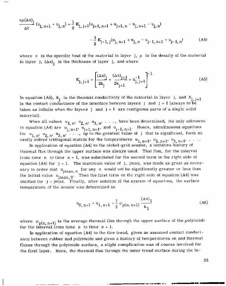
where c is the specific heat of the material in layer j , p is the density of the material in layer j , (Ax). is the thickness of layer j , and where

J

In equation (A5), k.J

is the thermal conductivity of the material in layer j , and hj , j + l

is the contact conductance of the interface between layers j and j + 1 (always to be taken as infinite when the layers j and j + 1 are contiguous parts of a single solid material).

When all values ul, n7 U 2 , n 7 u3, n, . . . , have been determined, the only unknowns in equation (A4) a r e u.

j, n+l’ ‘j+l, n+l’ and u.J -1,n+l’ Hence, simu Itaneous equations

for u l , n ? U 2 ,n’ U 3,n’ * * . , up to the greatest value of j that is significant, form an

easily solved tridiagonal matrix for the temperatures ul, n+17 u2, n+l, u3, n+l, . . . . In application of equation (A4) to the nickel-grid sensor, a tentative history of

thermal flux through the upper surface w a s always used. That flux, for the interval from time n to time n + 1, w a s substituted for the second term in the right side of equation (A4) for j = 1. The maximum value of j , jmax, w a s made as great as neces­s a r y in order that ujlnax, for any n would not be significantly greater or less than the initial value ujmax, o. Then the f i r s t term on the right side of equation (A4) w a s omitted for j = jmax. Finally, after solution of the system of equations, the surface temperature of the sensor w a s determined as

where cpP b , n+l) is the average thermal flux through the upper surface of the polyimide for the interval from time n to time n + 1.

In application of equation (A4) to the t i re tread, given an assumed contact conduct­ance between rubber and polyimide and given a history of temperatures on and thermal fluxes through the polyimide surface, a slight complication was of course involved for the f i r s t layer. Here, the thermal flux through the outer t read surface during the in­

35

terval from time point n to time point n + 1 is composed of two parts, according to equation (1). One of those par ts cpC(,, n+l) is conductive flux through the contact con­ductance from the polyimide surface; the other cprf(n, n+l) is friction heat generated on the rubber surface. Neither cpC(,, n+l) nor Vrf(n, n+l) is known. However, we may

use resul ts from the thermal analysis for the nickel-grid sensor, namely, cpp(n, n+l) and the average temperature of the polyimide surface during the interval from time point n to time point n + 1, u ~ ~ ( ~ ,n+l).

Implicit in equation (1) is the following equation:

A finite -differ ence analogue of that equation is

where qf(n,n+l) is the average rate of heat generation by friction on both sides of the interface between polyimide and rubber during the interval from time point n to time point n + 1, and U O r ( n , n + l ) and u

Op(n, n+l) a r e the average temperatures on rubber

surface and polyimide surface respectively during the same interval. The only unknowns in equation (A8) a r e qf(n,n+l) and u ~ ~ ( ~ ,n+l). We may eliminate g(t) from equations (1) and (A7), giving

A finite-difference analogue of equation (A9) is

where qr(n, n+l) is average rate of flow of heat into rubber surface during the interval from time point n to time point n + 1. Now, for j = 1, we may substitute the positive left side of equation (A10) for the negative second te rm in the right side of equation (A4), giving

36

I

Equation (Al l ) has three unknowns, namely, u ~ ~ ( ~ ,n+l), ul , n+l, and u2, n+l. This equation, then, is suitable for the second row in our tridiagonal matrix. But w e need an equation for the f i r s t row of the matrix containing only u ~ ~ ( ~ , u l , n + l asn+l) and unknowns. Such an equation may be easily obtained by substituting

1 n n + l j

2kr for i ts approximate equivalent qr(n,n+l) in[UOr(n,n+l) - ( ~ 1 , + ~ 1 ,

equation (AlO), giving

(Here we use kr instead of krs because krs applies only as far down as the depth of surface asperities. The depth to which kr applies in eq. (A12) amounts to one half the thickness of the uppermost layer of rubber. ) So equation (A12) for the f i rs t row, equa­tion (Al l ) for the second row, and equation (A4) for subsequent rows, make up a t r i ­ diagonal matrix that can readily be solved for u.

J , n+l for j 2 1 and for u ~ ~ ( ~ , ~ + ~ ) .

Equation (A10) may then be solved for qr(n,n+l). Finally, equation (1) may be solved for g(t).

37

APPENDIX B

RECONCILIATION OF RECENT RESEARCH AT UNIVERSITY OF MICHIGAN

WITH THIS REPORT

Reference 3 came to the author's attention after this report was written and after his retirement, but before publication of this report. Rather than undertake substantial revision of the body of this report to include analysis and discussion of reference 3 wherever pertinent, it was decided to res t r ic t such analysis and discussion to this ap­pendix. Such analysis and discussion wil l begin with the question of depth at which heat is generated by friction.

NATURE OF GENERATION OF HEAT BY FRICTION

A part of reference 3 that is vital to the present report is Section VI, entitled GENERATION OF HEAT DUE TO SURFACE EFFECTS. This section of reference 3 is directed toward a theoretical estimation of the effective depth beneath a rubbing su r ­face a t which friction heat is generated and toward the question of the fraction of the total friction heat generated within each of two different materials when their surfaces a r e rubbed together.

Equation (1)w a s derived in reference 1under the theory that the heat of friction is generated within the surface layers of atoms or, at most, just a few atomic layers beneath each surface. If, instead, the friction heat were generated at a substantial depth beneath either surface, then equation (1)would not be valid and the entire analysis reported here would have to be carefully re-examined as to whether its results a r e significant.

Theories about the cause of friction and the manner of generation of heat by fr ic­tion a r e st i l l controversial. Probably the oldest theory that still has i ts adherents is that of Coulomb. According to Coulomb's theory, mutual adhesion of the rubbing sur ­faces plays only a minor role, if any, in friction. Instead, this theory holds that f r ic­tional force is caused by the action of myriads of asperit ies on the two surfaces climb­ing up on each other like pa i rs of mating wedges. Such wedging action would require an equilibrium between force vectors normal to the gross surfaces and force vectors tan­gential to those surfaces. According to this theory, the net effect of these many minute tangential vectors constitute the frictional force.

According to this theory, generation of heat would be due to hysteresis involved in the repeated deformation and relaxation of material at substantial depths beneath the

38

surface, caused by the localized wedging action. The derivation of equation (1) (eq. (B12) in ref. 1)would not be valid.

According to more modern theory, asperit ies have little effect except to account for the fact that the effective rubbing a r e a varies as the normal load between two metals, or as a power of the normal load somewhat l e s s than unity when a polymer is involved. According to this theory, as clearly explained recently by Merchant (ref. lo), the f r ic­tional force is caused mainly by adhesion between surface atoms of the two rubbing ma­terials, though some frictional force may be caused by asperit ies on the harder surface "plowing" through the softer surface. The atomic adhesion does not require the pres­ence of asperities, except that the individual adhering atoms themselves might be r e ­garded as asperities.

Defense of the Coulomb theory w a s presented by Bikerman in his discussion of In that discussion Bikerman freely acknowledged that theMerchant's report (ref. 10).

adhesion theory represents the majority view, as did Ku in his later nonpartison dis­cussion.

The present author can add little indeed to the discussions among Merchant, Biker-man, Ku, Tabor, and others when he states that he himself adheres to the adhesion theory and consequently believes that his equation (eq. (1))is approximately correct.

Clark and Staples in reference 3 report about the same coefficient of friction (1.4) for a rubber t i re on a smooth d r y aluminum surface as on a dry concrete or asphalt surface. Such a comparison seems to suggest little effect indeed from "plowing" of asperit ies through the rubber. If the "plowing" contribution to friction were substan­tial, we should expect a much greater coefficient with concrete or asphalt than with smooth aluminum.

In figure 16 a single asperity on a hard supporting surface is shown for simplicity as a right prism of isosceles triangular cross section whose axis is perpendicular to the plane of the figure and extends at right angles to the direction of slide of the rubber surface above it. Adhesion between rubber and solid material is assumed nonexistant, s o that the only forces exerted by the prismatic asperity on the rubber a r e Pnl and Pn2, each normal to a surface of the prism. These two forces a r e resolved into com­ponents P1 and F1 on the uphill side of the prism and components P2 and F2 on the downhill side of the prism.

Because of the hysteresis loss factor 17 used by Clark and Staples, we may write

The net frictional force exerted by the asperity against the motion of the rubber wi l l be

F = F 1 - F2

and the total upward reaction of the asperity against the load will be

P = P1 + P2

The tangent of each of the angles p shown in figure 16 wil l be

p1 p2

The coefficient of friction must be

Fp = -P

Solving equations (Bl) to (B5), we get

t a n p = - p 036)17

Note that the value of p given by equation (B6) must exist for the average asperity if the sliding friction coefficient p is to exist. If we use the coefficient 1 . 4 found by Clark and Staples and a value 17 = 1/2 which is probably unreasonably large, we get about 76. 5' for the value of p. Even with 17 = 0. 9, /3 = 59.7'. Williamson (ref. 11) found that typical asperities on surfaces of solids have slopes occasionally as steep as 25' but that the slopes a r e usually between 5' and 10'.

It appears, therefore, that the Coulomb concept of friction is quite untenable for the rubber t i re sliding on a smooth aluminum surface.

The analysis by Clark and Staples on generation of heat by friction may have an ap­proximate application to the adhesion concept of friction. In considering such applica­tion we will, for the present, ignore the effect on heat generation due to the rupture of rubber-to-rubber bonds. As many rubber -to-aluminum bonds would be created exo­thermically as would be ruptured endothermically. The ruptures of rubber -to-rubber bonds would be extremely close to the rubber-aluminum interface. If, on the average, such ruptures occurred at depths of more than a few atomic diameters beneath the t read surfaces, treads would not last as long as they do. Moreover; rupture of rubber-to­

40

rubber bonds must be endothermic. The treatment by Clark and Staples ignores forces normal to the rubbing surfaces

and apparently does not need to take those forces into account for its purposes. Mathe­matical expressions a r e developed for s t resses and strains within a semi-infinite solid whose surface is infinitely smooth. The s t resses and strains a r e treated as being caused by intermittent (stick-slip) movement of a minute asperity of the other body along the infinitely smooth surface. That is, a model is used according to which a frictional force is intermittently applied, tangentially to the infinitely smooth surface, along a line that lies in the surface at right angles to the direction of the force.

Such a model corresponds with the atomic interactions presumed to generate f r ic­tional heat by Tabor in one of his responses to Bikerman in the discussion of Merchant's report (ref. 10). It is true that an atom displaced by adhesion does not correspond to the line application of a force assumed by Clark and Staples, but a line of adhering atoms within the surface could be considered without undue violence to the adhesion con­cept of friction.

According to this model, Clark and Staples developed the following equation for dif­ferential heat generation for a single cycle of application of the force:

2d Q = a . dx

4i7E x

where P is the tangential force, E is modulus of elasticity, and x is distance be­neath the surface.

The d.efinite integral of equation (B7), for total heat generation occurring at all depths between x1 and x2 is

2 a x 1 < x < x2) = 9In($)4i7E

This equation has the obvious faults that a x 1 < x < x2) approaches infinity as x2 approaches infinity or as x1 approaches zero. Hence, the range of values of x throughout which the equation may be applied is subject to judgment and the practical value of the equation is consequently somewhat limited.

A related limitation of the usefulness of equation (B8) as applied to a stick-slip phenomenon is due to the fact that its derivation involved the implicit assumption that the force P is applied long enough that a steady-state distribution of strains and s t resses is achieved. For such a steady-state distribution at an infinite depth x2 the force P would have to be applied for infinite time. Clearly, equation (B8) could not be used with a greater value of x2 than the depth to which a transverse wave could travel during one cycle of application of the force P.

41

The adhesion of atoms at the surfaces of contact for extremely short intervals of time could cause an approximation of the steady-state distribution of s t resses and strains only at very shallow depths. An exact solution of the problem dynamically would require a major mathematical effort, which cannot be undertaken here. The so­lution would have to involve treatment of an infinite s e r i e s of transverse waves traveling from the surface into the depths of the rubber, with due regard to the attenuation of each wave at every depth because of mechanical hysteresis. However, a useful approx­imate solution seems to be possible with use of equation (B8)if we use for x2 the depth to which a transverse wave could travel during one cycle of application of force. Ne­glect of heat generated at depths greater than x2 because of the eventual travel of transverse waves to greater depths should not be too serious because of the very large value of q for tread rubber. Also, such neglect would be countered by the fact that s t resses and strains resulting from transient surface forces would tend to be concen­trated at positions nearer the surface than called for by equation (B7).

We may gain some conception of the ease or difficulty involved in the flow of heat to the rubbing surface, from the depths at which it is generated according to equation (B7), by considering two imaginary conditions as follows: (1)the heat is generated according to equation (B7),but is all compelled to flow to the surface because of a plane parallel to the rubbing surface and having zero conductance, at the depth x2; and (2) the same quantity of heat is generated at an effective depth xe, and it is all compelled to flow to the surface by a plane parallel to the rubbing surface and having zero conductance, at a depth infinitesimally deeper than xe. For the purpose of the comparison, we wil l as­sume that the temperature reached at depth xe for condition (2) is equal to the average temperature reached within the region between x1 and x2 for condition (1).

For the imaginary condition (l),if we assume that enough cycles of heating accord­ing to equation (B8)have occurred for a virtual steady-state temperature distribution to exist, then

where u is the temperature at distance x below the surface and f is the frequency of the stick-slip cycle. From equation (B9),

47rE

We may now obtain an average temperature for imaginary condition (1) as

42

-T = a

with use of equation (B10) for u and equation (B7)for dQ. Thus,

2(x2 - XI)

f:) But the temperature reached at depth xe under imaginary condition (2) must be

Substituting from equation (B8) into equation (B13), then equating Ta and Tb, and solving equations (B12) and (B13), we get

As we must not make x1 equal to zero, probably a minimum reasonable value for i t would be about half the diameter of a carbon atom or about 9X10-8 mm.

For use in estimating a reasonable value for x2, we wi l l assume that, whenever a rupture of either a rubber-to-aluminum bond or a rubber-to-rubber bond occurs, the rubber atom wil l not have been displaced by more than about 10 diameters of a carbon atom, or about 1. 8X10-6 mm. We wi l l assume that the rubber is sliding relative to the aluminum a t 30 m/sec (98 .4 ft/sec).

We may compute the speed of a transverse (or a solenoidal) wave through the t read rubber with the following equation from reference 12:

v =Q 6where G is shearing modulus of elasticity, or rigidity. With a value range of 1 . 3 ~ 1 0

to 2.0XlO6 N/m 2 for G (values for polyisoprene vulcanized with 33 percent carbon black

43

from ref. 13) and with p = 1200 kg/m 3 (ref. 14), equation (B15) yields a value range for v of 32.9 to 40. 8 m/sec. We wil l use the approximate median of this range, 37 m/sec.

The time for travel through 10 diameters of a carbon atom a t 30 m/sec (98.4 ft/sec) would be 6x10-l1 sec. During that time, the t ransverse wave at 37 m/sec would travel approximately 2. 2X10-6 mm. Thus, 2. 2X1Ow6mm seems to be a reasonable value for x2.

With the values x1 = 9x10-8 mm and x2 = 2. 2X10-6 mm, equation (B14) gives us an effective depth of heat generation of xe = 2. 66X10-7 mm. This result puts xe within less than two diameters of a carbon atom from the rubbing surface. The res i s t ­ance to the flow of the heat through two layers of atoms or less should be quite negli­gible.

Clark and Staples conclude from equation (B8) and experiment that much more heat would be generated in rubber than in aluminum when one slides over the other. This author would not for a moment quarrel with that conclusion. In the discussion following equation (1)he stated that it represents an imaginary equivalent condition in which heat~~

generation occurs on the surfaces in proportion to their conductivities. No such r ea l condition w a s assumed or concluded to exist in the derivation of the equation in refer­ence 1. Instead, under the assumption that the heat w a s generated practically within the surface layers of atoms, it w a s considered that it could flow from the surface of one asperity to the surface of another asperity (in the other material) with only negligible contact resistance. The result is the same as if the heat had been generated at the roots of the asperit ies in proportion to the conductivities.

Gross stick-slip conditions unquestionably exist. Such conditions a r c necessary, for example, to explain the jagged curves for ra te of heat generation in figures 9 to 12. Stick-slip is thought to be due to the fact that static friction is usually greater than slid­ing friction. The stick-slip condition is usually associated with a vibratory system that involves oscillation of all or par t of the rubbing surface fore and aft in the direction of sliding. The vibration may be far from sinusoidal. Whatever the velocity of the slide, a vibrational amplitude might exist at which the maximum backward velocity of the s u r ­face due to the vibration is equal to the forward velocity of the slide. Static friction then exists momentarily once during each cycle of oscillation and causes energy to be fed into the vibratory system. The stick-slip condition terminates when the sliding velocity requires an excessive oscillatory amplitude, which ruptures part of the vibrating sys­tem, makes it very nonlinear, or causes it to dissipate energy more rapidly than the static friction can feed energy into it.

The stick-slip condition shown by the curves for ra te of heat generation in figures 9 to 12 must surely have caused some heat generation deep within the rubber. That heat, however, would not have had time to flow appreciably through the rubber to the temperature sensors. Consequently, it could not have formed an appreciable part of

44

the 64 percent of total heat estimated to be caused by the type of slippage known as squirming. It seems, therefore, that little leeway exists for the supposition of a sub­stantial amount of heat generation by the gross stick-slip condition. Only 36 percent of the total drag of the t i re w a s ascribed to the effect of hysteresis. The minute distortions of the rubber caused by sticking of elements of i ts surface several times during a total movement of only 1. 5 mm could scarcely compare with the gross cyclic distortions of the rubber caused by the large flat spot in contact with the supporting surface. Hence the heat generation within the rubber due to the stick-slip action could be only a small par t of the 36 percent.

From the foregoing analysis and discussion, it appears that the treatment of this subject by Clark and Staples, in conjunction with the analysis presented here, has helped considerably to demonstrate that heat of friction is generated mainly within the surface atoms of rubber and that it should be possible to dissipate it rapidly from that surface according to equation (1) with use of a supporting material of high thermal conductivity. (I am informed that the f i r s t author of ref. 3 does not agree with this statement. I do not know whether the second author is yet aware of the statement. ) Additional evidence from their report as to the efficacy of an aluminum surface for that purpose wil l now be dis­cussed.

DISSIPATION OF FRICTIONAL HEAT FROM RUBBER TO HIGHLY

CONDUCTIVE MATING SURFACE

Clark and Staples in reference 3 report a summary of tests involving the sliding of a t i re with locked wheel on a s t r ip of aluminum sheet approximately 6. 1 m (20 ft) long and 0.48 mm (0 .019 in. ) thick. They report the a rea of the contact patch as 380.6 cm2

(59 in. 2, and the length as 30 cm (11. 8 in.) . The width of the contact patch, then, should have been 12. 7 cm (5 in. ). They report that a temperature r i s e of 44.4 K (80' F) w a s measured on the surface of the contact patch at the end of the slide, with a load of 4450 N (1000 lb) and velocity of 0.643 m/sec (2. 11 ft/sec).

It is known (ref. 7) that substantially uniform temperature wi l l be reached through­out the depth of a layer of metal, with a constant heat flux through the surface, if

& > 1 z 2

where 1 is thickness. For aluminum, with diffusivity of 8. 5 8 ~ 1 0 ~ ~m2/sec, contact duration of 0.466 sec, and 2 = 0.48 mm, this criterion w a s far exceeded in the tes ts reported by Clark and Staples with at/Z2 = 174.

45

With the normal load of 4450 N and coefficient of friction of 1.4, the work done against friction Wf for each meter of slide was 6230 J. The mass of aluminum heated during 1meter of slide must have been the product of that meter by the width w of the contact patch, the thickness 2 of the aluminum sheet, and the density of the aluminum

pal. The temperature elevation then, under the optimistic assumption that all the heat generated by friction went into the aluminum, would have been

AT = wf

With the specific heat cal = 865 J/(kg)(K) and pal = 2700 kg/m 3, equation (B17) gives a temperature r i se of 43.8 K.

This result agrees remarkably well with the temperature r i s e of about 44.4 K on the tread surface reported by Clark and Staples. Under the assumption that virtually all the heat flows into the aluminum, with very high contact conductance, the maximum temperature of the rubber surface (at the trailing end of the contact patch) immediately after the slide should be only slightly higher than the temperature reached by the alum­inum. The fact that the maximum temperature reached by the rubber surface w a s just 0.6 K higher than the calculated temperature that should have been reached by the aluminum is another verification of the theory that the heat of friction is generated al­most wholly on the surface of the rubber and can flow almost entirely into a highly con­ductive supporting surface. This result also indicates that thermal contact resistance between tread rubber and aluminum is not great enough to be a substantial impediment to the dissipation of most of the friction heat into the aluminum. The result also sup­ports the earlier assumption that the endothermic rupture of rubber-to-rubber bonds does not account for a substantial fraction of the energy consumed.

Note that the temperature r i se of the rubber surface i s theoretically not affected by the velocity of the slide so long as the criterion (B16) is satisfied. With thicker alum­inum surfaces, however, substantial heat could be conducted away from the rubber even if this criterion were far from satisfied.

Also note, in view of the close agreement of the t i re surface temperature r i s e r e ­ported by Clark and Staples with the calculated temperature r i s e for the aluminum from equation (B17), that the t i re could have been slid much farther without subshntially greater r i se of i ts surface temperature.

THERMAL CONTACT CONDUCTANCE

Clark and Staples in reference 3 estimated a value of thermal contact resistance. They designated their result as R* and called it a "heat flux impedance coefficient",

46

emphasizing that "it is a measure of contact resistance but it is not the contact res is t ­ance. '(

They heated a par t of the tread surface of a stationary t i re greater than the antici­pated contact a r e a with heat lamps. They then repeatedly rolled the heated portion of the tread over temperature sensors, making records of the resulting temperature his­tories of the sensors. From the rates of temperature r i s e of the sensors during the early par t of the contact, with use of independent calibrations of the sensors, they de­duced values o� %.

Their results for R, for two independent sensors were equivalent to conductances of 1.&lo4 and 2 . 4 ~ 1 0 ~W/(m2)(K) or 2. 4x103 and 4. 2X103 Btu/(ft2)(hr)(OF). It w a s tempting for this author simply to point out that these values a r e within the range of pos­sible contact conductances that he found from his study of figure 13. But after careful study of the sensor design, the method of test, and the results reported in reference 3, he regretfully concluded that this method cannot indicate the contact conductance with sufficient accuracy to be of much value.

The sensors used by Clark and Staples were aluminum disks to the under sides of which had been cemented resistance thermometers just like that illustrated in figure 1. Each disk w a s isolated from contact with anything but the t read surface, with the excep­tion of a hollow plastic cylindrical pedestal, which supported the periphery of the alum­inum disk from underneath.

This author subjected the system (tread rubber-aluminum disk-resistance thermom­eter) to runs of the same type of finite-difference computer program that has been de­scribed. He used a ser ies of assumed values of contact conductance between tread rub­ber and aluminum disk. He assumed the aluminum disk and the resistance thermometer to be at a uniform temperature before contact, and assumed the tread rubber to be at a uniform temperature 40 K ('72' F) higher. The computer program yielded rates of tem­perature r i se during the f i r s t 50 to 100 msec for the nickel grid within the resistance thermometer.

For an assumed infinite contact conductance, the result w a s 71. 1 K/sec (128' F/ sec). For the same initial temperature difference of 40 K (72' F), Clark and Staples "sensor 2" showed a rate of temperature r i s e of 67.3 K/sec (121' F/sec). Thus, ac­cording to the finite-difference program, their sensor 2 showed an almost infinite con­tact conductance. For an assumed contact conductance of 3500 W/(m )(K), the computer2

program showed a temperature r i s e of 40 K/sec (72' F/sec). Clark and Staples "sen­sor 1" showed a ra te of 39.9 K/sec (71. 8' F/sec). Hence, according to the finite-difference program, their sensor 1 indicated a contact conductance of only 3500 W/

(m2)(K). The rates of temperature r i s e f rom the computer program should both be expected

to be too high, because of it w a s necessary to ignore heat that would flow from the alum­inum disk to the supporting plastic pedestal. That is, if the computer program could

47

have yielded the correct ra tes of temperature r i se for the assumed values of contact conductance, then somewhat higher contact conductances would have had to be assumed to match the rates found by Clark and Staples. It is believed this effect would be very small.

In the treatment of the results by Clark and Staples, it apparently was necessary for them to regard the thermal contact resistance as being the only impediment to heat flow for a period of 50 to 100 msec. Actually, in far less than 50 msec, substantial temperature gradients develop within the rubber, the aluminum disk, and the resistance thermometer. Because of these gradients, the actual temperature difference available to drive heat through the contact resistance between rubber and aluminum drops to a low value in much less than 50 msec and the heat f lux becomes largely a function of the gradients rather than a function of contact resistance. This fact is clearly demonstrated by the computer result indicating a temperature r i s e ra te for the nickel grid of only 71. 1K/sec (128' F/sec) even with infinite contact conductance.

The enormous difference between the conductances found from the two sensors with use of the finite difference program precludes the placing of much value on the results. This author is at a loss to explain the difference, except possibly with the suggestion either that sensor 1 did not have a good thermally conductive bond between the aluminum disk and the resistance thermometer, or that sensor 1had a much thicker layer of ce­ment between the disk and the thermometer than did sensor 2. (The conductance of the bond between the aluminum disk and the resistance thermometer used in the computer program was 4800 W/(m 2)(K), the same as earlier found for each of the bonds between polyimide and nickel grid. ) Note that no such possible failure to achieve a good ther­mally conductive bond between sensors and asphalt for the tests reported in reference 2 could have affected the analysis of those test results that has been reported here. Even with the assumption of infinite contact conductance between the resistance thermometers and the asphalt, the finite-difference program showed only negligible heat entering the asphalt from the polyimide of the resistance thermometer.

48

REFERENCES

1. Miller, C. David; and Pinkel, I. Irving: Aluminum Runway Surface as Possible Aid to Aircraft Braking. NASA T N D-7186, 1973.

2. Nybakken, G. H.; Collart, D. Y.; Staples, R. J.; Lackey, J . I . ; Clark, S. K . ; and Dodge, R. N. : Preliminary Measurements on Heat Balance in Pneumatic Tires. (DRDA 036390-2-T, University of Michigan; NGR 23-005-417. ), NASA CR-121349, 1971.

3. Clark, S. K. ; and Staples, R. J. : Friction and Temperature Rise in Aircraft Tires. (DRDA 036390-3-F, University of Michigan; NGR 23-005-417. ), NASA CR-134666, 1974.

4. Abraham, Herbert: Asphalts and Allied Substances. Vol. 4 - Methods of Testing Industrial Raw Bituminous Materials. 6th ed., D. VanNostrand Co., Inc., 1963.

5. Baumeister, T. ; and Marks, Lionel S.: Mechanical Engineers Handbook, McGraw-Hill.

6. Perry, John H. ; Perry, Robert H. ; Chilton, Cecil H. ; and Kirkpatrick, Sidney D. : Chemical Engineers Handbook. 4th ed., McGraw-Hill, 1963.

7. Carslaw, Horatio S. ; and Jaeger, J. C. : Cond.uction of Heat in Solids. 2nd ed., Oxford, Clarendon Press , 1959.

8. Miller, C. David Distribution of E r r o r in Least-Squares Solution of an Overdeter­mined System of Linear Simultaneous Equations. NASA TN D-6744, 1972.

9. Richtmyer, Robert D. ; and Morton, K. W.: Difference Methods for Initial Value Problems. 2nd ed. , Interscience Publishers, 1967.

10. Merchant, M. E . : Friction and Adhesion. Interdisciplinary Approach to Friction and Wear, P. M. Ku, ed. , NASASP-181, 1968, pp. 181-266.

11. Williamson, J. B. P. : Topography of Solid Surfaces. Interdisciplinary Approach to Friction and Wear, P. M. Ku, ed. , NASA SP-181, 1968, pp. 85-142.

12. Page, Leigh: Introduction to Theoretical Physics. D. VanNostrand Zompany, Inc., 1935.

13. Brandrup, J . ; and Immergut, E. H., eds. : Polymer Handbook, Interscience, 1966.

14. Goldsmith, Alexander; Waterman, Thomas E. ; and Hirschhorn, Harry J. : Hand­book of Thermophysical Properties of Solid Materials. Vol. 4, Pergamon Press, 1961.

49

--- ---

TABLE I. - TOTAL RATE OF HEAT FLOW THROUGH

BOTH INNER AND OUTER SURFACES OF TIRE

TREAD AT VARIOUS ELAPSED TIMES

AFTER START OF TEST -i Elapsed m2j' Rate of flow of heat

time, K/m out of tread, sec H .

OJ ' W - ~

0 0 0.0 (assumed) 1 40 445 130 45.16

70 28.0(by double interpolation) 2 100 667 348 80.4 3 180 778 1000 143.0 4 240 778 1610 193.6 5 480 1220 1350 206.2 6 720 1000 1850 330.6 7 960 1160 2000 255.4 3 1200 778 2580 274.0 3 1440 1390 2580 $21.2- ~~ -~

TABLE rr. - WHEEL DRAG FORCES NECESSARY TO PROVIDE ENERGY DISSIPATED

BY TREAD HYSTERESIS AT VARIOUS TIMES AFTER START OF TEST

AT 22.4METERS PER SECOND - .­

i Elapsed Rate of flow Median of Average Length oj iate of tread Hysteretic time, of heat out time inter- tempera- time in- hysteretic drag of tread

-~

'oi,W

start of test), sec

ATi, K

sec tion,

Hhi7

N Ib

W - -

~~

1 40 22.6 20 4.0 40 1680 75.16 16.90 2 100 62.8 70 4.5 60 1306 58.43 13.13 3 180 112.0 140 5.4 80 1231 55.08 12.38 4 240 168 210 4.4 60 1384 61.92 13.92 5 480 200 360 7.8 240 739 33.06 7.44 6 720 218 600 4.8 240 550 24.61 5.53 7 960 243 840 2.5 240 416 18.61 4.18 8 1200 265 1080 1.4 240 362 16.20 3.64 9 1440 298 1320 1.6 240 409 18.30 4.11

sec of tread, val i (from ture rise, terval i, ieat genera-

- -~

50

Nickel r 0.005 0.0127 \ (0.0002) (0.0005) \ \

I 1 0.0254 (0.00 10)

Figure 1. - Detai l of sensor construction, ( A l l dimensions in mm (in.).)

I,r 0.020 sec

Figure 2. - Temperature-time records shown by two nickel-grid sensors when traversed by t i re that hsd been i n contact w i th pavemest for 30 meters or less (ref. 2).

5 1

I 1 AXjt1 _- / - - -Layer j.1 in rubber

(---Layer j in rubber

-16 K

Figure 3. - Temperature-time records shown by two nickel-grid sensors when traversed by t i re that had been ro l l ing under load for 2 to 3 kilometers (ref. 2).

) L-RUbber

I1-AXjt1 _- / - - -Layer j.1 in rubber Axj =-uj, here

(---Layer j in rubber

1 T I

-__- - -_!--Heat flow in to rubber pr(n, tl) -_*­

\

--Polyimide/ 1 ,n t l here ' I

+ '. '. . 'L Polyimide f r i c t ion heat generated here pp(n,

j-1, j-.-Layer j in sensor

~,-Polyimide ..--u. I. n here '-Layer j + l in sensor

Asp ha1t /_-I /\

Figure 4. - Generation of heat w i th in interface between surface of rubber t i r e and surface of temperature sensor, flow of heat, and entities used in numerical analysis.

52

,= Temperature record E- from nickel g r id 3 0 E E-. 1 E-.2

.-.

0 2 4 6 8 10 12 14 16 18 20

,-Estimated start E* of contact 3 ­; ; ;8 1- ,-Estimated end of contact

-Temperature of uppermost sensor surface relative to its in i t ia l temperature

I

-11 I 3

Thermal f lux through

of nickel g r id calculated by

-2 f i n ite-diffe rence comouter o rwram

.IC l - Temperature record-3 m,= .1 I..

E- from nickel g r id3 0.-.EE-.1 E-.2

0 2 4 6 8 10 12 14 16 18 20 Time, msec

Figure 5. -Temperatures of upper surface and thermal fluxes into upper surface of nickel-grid sensor derived from temperature record of nickel g r id for trace 1, in figure 2.

/’7 Estimated start of contact

_--Estimated end of contact.-Tempe rat u re of uppe rmost sensor surface relative to

1 its in i t ia l temperaturen

Thermal f lux through uppermost surface in to sensor

c

0 Temperatures of nickel g r id calculated by finite-difference computer program

II I -Temperature record

2 4 6 8 10 12 14 16 18 Time, msec

Figure 6. -Temperatures of upper surface and thermal fluxes in to upper surface of nickel-grid sensor derived from temperature record of nickel g r id for trace 2, i n figure 2.

20

c

x

c

3i1,estimated start of contact

---Estimated end of contact -I I,,-Estimated start 5x104 .E z Temperature of uppermost

E' of contact 5 2 sensor surface relative to

,.-Estimated end of contact 4-8% i ts in i t ia l temperature

3­-Temperature of uppermost -2­sensor surface relative to N

Eits in i t ia l temperature -.-.3 1- Thermal f lux through L' uppermost surface in to sensor 0YI 0- 7Thermal f l u x through W

uppermost surface in to sensor m 0 c -1­.-c 3- -2-L-

\ -3- E

o Temoeratures of nickelo TemDeratures E

of nickel +-

-4- 3 -&' E \

g i i d calculated by .u 3 =l g i i d calculated by

finite-difference -5- w w .-> a finite-difference

computer program 5 : computer program Temperature record -6- 8- Temperature record

I from nickel g r id I I I -7 - J I from nickel g r id

10 12 14 16 18 20 0-2 4 6 8 10 12 14 16 18 20 Time, msec Time, msec

Figure 7. -Temperatures of upper surface and thermal fluxes in to upper surface Figure 8. -Temperatures of upper surface and thermal fluxes into upper surface of nickel-grid sensor derived from temperature record of nickel g r i d for trace 3, of nickel-grid sensor derived from temperature record of nickel g r id for trace 4, in f igure 3. i n f igure 3.

3

I

3

-1

-4

- 5

" um .+.. L

CA

a, n aI

c 0

3 x l d

0

O [ -:t fI

-3 1 0

Temperature of rubber surface relative to in i t ia l temperature of polyimide surface (rubber surface temperature)

Temperature of rubber surface relative to that of polyimide surface (relative rubber surface temperature)

Conductive heat f l u x from polyimide surface to rubber surface (conductive f lux )

Rates of generation of heat by f r i c t ion on rubber surface, on polyimide surface, and total (rubber f r i c t ion heat, polyimide f r i c t ion heat, and total fr ict ion heat)

Figure 9. -Temperatures of rubber surface, conductive heat fluxes across polyimide-rubber interface, and rates of generation of heat by f r i c t ion for trace 1, wi th assumed contact conductance of 11315 Wl(m2KK) o r 2000 Btu l (ft2MhrH'FI.

55

-2

c

7x104

e

-1i0

1

Temperature of rubber surface relative to in i t ia l temperature of polyimide surface (rubber surface temperature)

Temperature of rubber surface relative to that of polyimide surface (relative rubber surface temperature)

Conductive heat f lux from polyimide surface to rubber surface (conductive f lux)

Rates of generation of heat by f r i c t ion on rubber surface, on polyimide surface, and total (rubber f r i c t ion heat, polyimide f r i c t ion heat, and total f r ic t ion heat)

-31 I I I I I 0 2 4 6 8 10

Time, msec

Figure 10. -Temperatures of rubber surface, conductive heat fluxes across polyimide-rubber interface, and rates of generation of heat by f r ic t ion for trace 1, wi th assumed contact conductance of 56 744 WI (m%K) o r 10 OOO Btu l (ft2)(hr)('F).

56

c

m

m

Y o r

14xJ P N --E 12 3

-.-0 10 c U._L L 8­xfl

6­

4 ­

2­c 0 0-W c E ­-2

--4

-6 I 0 2

Temperature of rubber surface relative t o in i t ia l temperature of polyimide surface (rubber surface temperature)

Temperature of rubber surface relative t o that of polyimide surface (relative rubber surface temperature)

Conductive heat f lux from polyimide surface to rubber surface (conductive f lux )

Rates of generation of heat by f r i c t ion on rubber surface, on polyimide surface, and total (rubber fr ict ion heat, polyimide fr ict ion heat, and total fr ict ion heat)

I-I._L.L-.! 4 6 8 1 0 Time, msec

Figure 11. - Temperatures of rubber surface, conductive heat fluxes across polyimide-rubber interface, and rates of generation of heat by f r i c t ion for trace 2, with assumed contact conductance of 11345 WI(m2KK) o r 2M)O Btu, (ft21(hrlf°FI.

57

Y 2 r c 0 w­2 % 0

L

zz ' t c .+

4.-3 w g c ' ZZ c g .- g 5a 't .E -4 ._ nL

.6x&JJ n3 A mE W E :mg4t+

s 3 sb

12C I

4

2

l l0

Temperature of rubber surface relative to in i t ia l temperature of polyimide surface (rubber surface temperature)

Temperature of rubber surface relative to tha t of polyimide surface (relative rubber surface temperature)

Conductive heat f l u x f rom polyimide surface t o rubber surface (conductive f lux)

Rates of generation of heat by f r ic t ion o n rubber surface, on polyimide surface, and total ( rubber f r i c t ion heat, polyimide f r i c t ion heat, and total f r i c t ion heat)

I-4u-6 I. ­

0 2 4 6 8 1 0 Time, msec

Figure 12. -Temperatures of rubber surface, conductive heat fluxes across polyimide-rubber interface, and rates of generation of heat by f r i c t ion for trace 2, with assumed contact conductance of 56 744 WI (mZ)(K) o r 10 OOO B t u l (fl2Nh rM0Fl.

58

0

Trace 0 1a 2 v 3

11 0 4

-5 I d I I I I L 3 x l d

Averageconductive flux

E;1

v 1C2 r L 6xId'

friction-;E]:::e I­

1 1 0 I 1 2 3 4 5 6 x l d

Contact conductance, WI (m2)(KI

Figure 13. - Calculated initial rubber temperatures, rates of heat conduction, and rates of heat generation by friction for assumed values of contact conductance throughinterface between polyimide and rubber.

I ,,-;ApproximateI I r y locations of plies

Elapsed time,

40

35

15

10 I

Inside wall b a d temperature, 281K (46' F) Air temperature. 278 K (400 F)

I I I 0 5 10 15 20

Depth from inside wall, m m Figure 14. -Temperature profiles a! crown.

59

I--__l..-_I- I I.I_ 0 200 400 600 800 1000 1200 1400

Time from start of test, sec

Figure 15. - Calculated values of wheel drag required to provide energy dissipated by mechanical hysteresis in tread rubber.

Direct ion Rubber of sl ide -

Hard supporting material

Figure 16. - Forces caused by asperity on rubbing surface.

60 NASA-Langley, 1976 E-8357

NATIONAL AERONAUTICS AND SPACE ADMINISTRATION

WASHINGTON. D.C. 20546 POSTAGE A N D FEES P A I D

~

N A T I O N A L AERONAUTICS A N D OFFICIAL BUSINESS

PENALTY FOR PRIVATE USE $300 SPECIAL FOURTM-CLASS R A T E SPACE A D M I N I S T R A T I O N

451 USMAIL

BOOK

170 0 0 1 C 1 U A 760107 S00903DS DEPT O F THE A I R F O R C E AF WEI\PONS L A D O r i R T O R Y ATTN: T E C H N I C A L L I B R A R Y ( S I J L ) K I P T L A N C APE NM 87117

“The aeronautical and space activities of the United States shall be conducted so as to contribute . . . to the expansion of human knowl­edge of phenomena ifa the atmosphere and space. T h e Administration shall provide for the w d e s t pructicuble and appropriate dissemination of information concerning its activities and the results thereof.”

-NATIONAL AERONAUTICSAND SPACE ACT OF 1958

NASA SCIENTIFIC AND TECHNICAL PUBLICATIONS TECHNICAL REPORTS: Scientific and technical information considered important, complete, and a lasting contribution to existing knowledge.

TECHNICAL NOTES: Information less broad in scope but nevertheless of importance as a contribution to existing knowledge.

TECHNICAL MEMORANDUMS: Information receiving limited distribution because of preliminary data, security classifica­tion, or other reasons. Also includes conference proceedings with either limited or unlimited distribution. -CONTRACTOR REPORTS: Scientific and technical information generated under a NASA contract or grant and considered an important contribution to existing knowledge.

TECHNICAL TRANSLATIONS: Information published in a foreign language considered to merit NASA distribution in English.

SPECIAL PUBLICATIONS: Information derived from or of value to NASA activities. Publications include find reports of major projects, monographs, data compilations, handbooks, sourcebooks, and special bibliographies.

TECHNOLOGY UTILIZATION PUBLICATIONS: Information on technology used by NASA that may be of particular interest in commercial and other-non-aerospace applications. Publications include Tech Briefs, Technology Utilization Reports and Technology Surveys.

Details on the availability of these publications may be obtained from:

SCIENTIFIC AND TECHNICAL INFORMATION OFFICE

N A T I O N A L A E R O N A U T I C S A N D SPACE A D M I N I S T R A T I O N Washington, D.C. 20546