a fact of life: predictable returns from an equilibrium
TRANSCRIPT

A FACT OF LIFE: PREDICTABLE RETURNS FROM AN
EQUILIBRIUM MODEL WITH UNPREDICTABLE FUNDAMENTALS
Neal Maroney The University of New Orleans
College of Business Administration New Orleans, LA. 70148
and
Aris Protopapadakis University of Southern California
The Marshall School of Business, FBE Los Angeles, CA. 90089-1427
December 22, 2005
We want to thank Costas Azariadis, Giorgio De Santis, Mark Flannery, Ayse Imrohoroglu, Selo Imrohoroglu, Douglas Joines, Krishna Kumar, Fulvio Ortu, Rodney Smith, Richard Sweeney, Paul Zak, participants of the University of New Orleans Finance seminar, the University of Santa Barbara economics seminar, and the USC macro/international and finance workshops.

Revised 12/30/05 10:23 PM
2
A FACT OF LIFE: PREDICTABLE RETURNS FROM AN
EQUILIBRIUM MODEL WITH UNPREDICTABLE FUNDAMENTALS
December 22, 2005
We want to thank Costas Azariadis, Giorgio De Santis, Mark Flannery, Ayse Imrohoroglu, Selo Imrohoroglu, Douglas Joines, Krishna Kumar, Fulvio Ortu, Rodney Smith, Richard Sweeney, Paul Zak, participants of the University of New Orleans Finance seminar, the University of Santa Barbara economics seminar, and the USC macro/international and finance workshops.

ABSTRACT
We show that even when “fundamentals” are i.i.d., a three-period OLG competitive model
produces negatively autocorrelated expected returns, market risk premia, and prices;
conventional models deliver zero autocorrelation for the same fundamentals. The negative
autocorrelation we find arises out of market interactions among consumers that are ex-ante
identical but differ by age. This negative autocorrelation is pervasive in our model and persists
regardless of the autocorrelation structure of the “fundamentals”. Thus the model provides a
simple alternative explanation for the observed autocorrelation of returns. A byproduct is low
correlation between aggregate consumption and wealth, a puzzle for conventional models.

1
I. INTRODUCTION
A large number of “puzzles” have been documented in the finance literature in the last two
decades, including but not limited to the excess volatility, equity premium and risk-free rate
puzzles; these “puzzles” are not necessarily independent. “Puzzles” are defined with respect to
the dominant paradigm, in this case the infinitely-lived, representative consumer (ILRC) model.
Time variation and predictability of returns have recently become central and controversial.
There is also ample evidence that the correlation of wealth and aggregate consumption is far
lower than predicted by the ILRC model.
Evidence strongly indicates returns are positively autocorrelated over intervals of less than one
year (momentum) and increasingly negatively autocorrelated over longer horizons.1 This
empirical result has been debated extensively. However, in a recent paper Daniels (2003)
derives a most-powerful test and shows that most of the early rejections of long-horizon
predictability are due to the low power of the tests used. Lettau and Ludvigson (2004)
conclude that there is a strong mean-reverting transitory component in wealth, dominated by the
stock market. They also show that the correlation between wealth and aggregate consumption
is low, because most of the variation in wealth is transitory.
The simple infinitely-lived representative consumer model cannot account for time-varying,
negatively autocorrelated returns, nor can it account for the observed low correlation between
wealth and consumption. Understandably, many economists are skeptical of empirical findings
that cannot be explained with the standard paradigm. Thus, while the empirical evidence was
1 Summers (1986) shows that returns tend to be negatively correlated over long horizons, and that random walk tests have low power against the alternative hypothesis of a slow mean-reverting component. Fama and French (1988) use Summers’ framework to show that predictable expected returns explain long horizon negative correlation. Variance ratio tests by Poterba and Summers (1988) and Lo and MacKinlay (1988) confirm the presence of this stationary component. They find that the negative correlation of returns strengthens with longer horizons. Jegadeesh and Titman (1993) and the momentum studies that followed, confirm the presence of a strong stationary component to asset prices in the near term. Lewellen (2002) finds momentum present even in well-diversified portfolios and argues that excess covariance explains momentum profits. Fama (2001) documents that expected equity returns have been declining over the last 50 years.

2
being debated, a separate strand of the literature attempted to extend the standard model to
“explain” the empirical findings. These attempts have not produced a generally-accepted
explanation.
We show here that in a simple overlapping generations (OLG) endowments model long-horizon
negative autocorrelation of returns is not a puzzle at all; rather it is a robust and natural outcome
of the market interactions of utility-maximizing consumers. The model we build is standard in
every way, except that consumers live for 3 periods. This fact dramatically changes the
properties of asset returns: they display excess volatility, and expected returns, risk premia, and
prices are negatively autocorrelated.2 A byproduct of this negative autocorrelation is a low
correlation between wealth and aggregate consumption. This contrasts with the infinite-lived
consumer and the 2-generation OLG models, where, under the same conditions, prices and
expected returns have zero autocorrelation, their volatility is constant, and consumption and
wealth are perfectly correlated.
. There are no frictions, informational asymmetries or other market imperfections in the model.3
The fundamentals --probabilities, endowments, and dividends-- are time independent and utility
functions are CRRA. These fundamentals deliver zero autocorrelation in prices and expected
returns in an infinitely-lived representative consumer model as well as a 2-generations
competitive OLG model. We also show that the properties of asset returns in this 3-generation
OLG model are qualitatively independent of the underlying autocorrelation of the fundamentals.
There is a paucity of alternative theoretical models that convincingly explain return
predictability.4 The standard infinitely-lived representative consumer (ILRC) model has
2 This model also produces risk premia that are an order of magnitude larger than those produced by the ILRC model. This feature is first documented in Constandinides Donaldson & Mehra (2002). 3 The young are endowed with the only consumption good and when they become middle-aged they are further endowed with risky assets that pay dividends the following period. There is no production or storage of the consumption good. 4 Many variables are found to predict returns, including the price-earnings ratio, dividend yields, and industrial production; most recent is the consumption-to-wealth ratio. See Lettau and Ludvingson (2001).

3
difficulty generating the discount factor variability necessary for a mean-reverting stationary
component in asset prices; aggregate consumption growth is unpredictable and too smooth to
explain return predictability.5
Returns would be autocorrelated in the ILRC model if stock market fundamentals were
autocorrelated at the required frequencies.6 However, the evidence clearly rejects this scenario.
Campbell and Shiller (1998), Cochrane (2001), and Fama and French (2001) find that while
dividend yields are strong predictors of future returns, dividends themselves lack predictability;
the observed properties of “fundamentals” cannot explain return predictability. The consensus is
that discount factor volatility rather than dividend volatility accounts for most of the observed
returns variation.7 Le Roy and Porter (1981) and Shiller (1981) show that returns are too
volatile when the discount factor is assumed constant; at the same time, empirical research
documents that returns are predictable. The connection between these observations is that like
thunder from lightning, excess volatility arises from return predictability.8
Models that do not assume imperfections (e.g., frictions, asymmetric information, differences in
utility and/or beliefs) or serially dependent fundamentals, introduce hidden state variables and
other non-separabilities to engineer predictability. Campbell and Cochrane (1999) model a
representative agent with a non-separable power utility. They introduce an unobserved
recession state variable, habit, into utility; consumption growth is i.i.d.9 Habit serves to
disconnect the elasticity of substitution from risk aversion. The discount factor is variable and
time-dependent because risk aversion increases as consumption approaches habit and declines
5 See Lettau and Ludvigson (2001). 6 As discussed in Campbell (2001), the models of Cecchetti, Lam and Mark (1990,1993), Kandel and Stambaugh (1991) require significant predictable changes in dividends to explain equity market volatility. 7 See Cochrane (2001) and the references therein. 8 Campbell and Shiller (1988) make this point. The equity premium puzzle is also related to predictability. Fama and French (2001) conclude that the reason the post 1950 equity premium is so high is that prices were too low at the beginning of this period. They find the market dividend price ratio is higher at the beginning of the period than at the end unrelated to the stream of dividends. They show that predictability cuts the equity premium roughly in half. 9 This builds on the work of Abel (1990) and Constantinides (1990).

4
as consumption moves away from habit. Risk premia are negatively autocorrelated over
business cycle frequency; they increase in recessions and decrease in expansions.
Constantinides and Duffie (1996) use heterogeneous agents differentiated by permanent
idiosyncratic income shocks; there is lack of full insurance. By engineering the patterns of
shocks to match desired outcomes, their model can replicate a variety of observed aggregate
behavior.10 They allow partial consumption insurance but design the idiosyncratic shocks so
that agents choose to not diversify away the shocks.11 As in Campbell and Cochrane (1999),
the introduction of this state variable in utility disconnects risk aversion and the elasticity of
substitution. McCandless and Wallace (1991) create autocorrelation in a perfect foresight
OLG model by using utility with satiation. As endowments change, the oscillation between
multiple solutions generates negative autocorrelation.
Samuelson (1958) was the first to study the effect of acknowledging that consumers are finite-
lived. Overlapping generations models provide a motive for actual trade, absent in
representative-consumer models. In a 2-generations OLG model, old consumers sell their
assets in exchange for consumption.12 When consumers live 2 periods, the excess supply of
assets is totally inelastic because the old (who supply the assets) have no alternative use for
them and will sell them regardless of price. Thus, prices play no role in asset allocation except
to convince the young to hold all the assets.
By contrast, in a 3-generations model, the middle-aged consumers have the opportunity to
consume and also rebalance their portfolios. Thus, the excess supply of assets available to the
10 Cochrane (1991) shows empirical evidence that full consumption insurance, implied by the representative agents’ equalizing marginal rates of substitution from state to state, fails in micro data. 11 This is accomplished by manufacturing high cross-sectional variance in consumption growth when market returns are low. Asset prices support the no-trade equilibrium they engineer. Superimposing a representative agent on an economy with this heterogeneity results in the cross-sectional consumption variance entering the economy -wide intertemporal marginal rate of substitution. 12 See McCandless and Wallace (1991) and Azariadis (1993) for discussions of non-stochastic OLG models.

5
young is price-sensitive, which makes returns predictable.13 We expect such a model to be a
better description of asset price behavior than the ILRC model because price-sensitive excess
supply of assets is a better representation of markets than price-inelastic excess supply.
The central intuition of our model is as follows. In any state, the young can purchase more
assets with their endowment and consume more, if asset prices are low. When they become
middle-aged, their assets pay dividends, leaving them relatively wealthy. They are wealthy
enough to finance their consumption today and to keep plenty of the new assets they receive for
consumption when they become old. To induce the middle-aged to part with some of their
assets, the current young have to pay high prices. Thus, low prices follow high prices. This
property holds regardless of the autocorrelation structure of the underlying “fundamentals,” and
it results in autocorrelated expected returns and risk premia.
One conclusion is that common perceptions of how markets “should behave”, which depend
heavily on the properties of ILRC models, do not apply in this more realistic trading
environment. It is the combination of multi-period finite lives and the competitive equilibrium
among agents with necessarily different horizons that creates these qualitative differences.
One may question if this negative autocorrelation is induced by our stationary binomial
specification. After all, in a 2-state time-invariant equilibrium, prices will either stay the same or
go up (or down). The example below shows that this structure of uncertainty does not
preordain negative autocorrelation in expected or unexpected returns. Consider a 1-period
risky asset in an economy with a time-invariant price distribution. Let the probabilities be state-
independent and 0.5. The asset pays d(g) in a g-state and d(b) in a b-state. There will be two
prices: P(g) (g-state) and P(b) (b-state), 4 possible returns: ( )( )
,gPgd
rgg = ( )( )
,gPbd
rgb =
13 The total supply of assets is fixed in our model. The “excess supply” is what the middle-aged offer for sale to the young.

6
( )( )
,bPgd
rbg = ( )( )
,bPbd
rbb = and 2 expected returns, ( ) ( )gbggg rrrE += 5.0 ,
( ) ( )bbbgb rrrE += 5.0 . In this equilibrium the autocorrelation of prices, expected returns, and
unexpected returns is zero, because the g- and b-states arrive at random.14 However, the
unconditional autocorrelation of observed returns is negative (=-0.50) as a direct consequence
of the 2-state nature of the model. But this shows that unconditional autocorrelation of actual
returns is the wrong quantity to focus on, because it does not reveal information about the
economic processes at work. We study the properties of expected returns and risk premia.
The paper contains five additional sections. In section II we state the individuals’ maximization
problem and the market clearing conditions. In section III we present the solutions and
properties of the benchmark models. In section IV we solve our competitive 3-period model,
and prove our main results. Section V contains simulation results that show the quantitative
importance of our results. It also contains comparisons to the benchmark solutions. Section VI
contains concluding remarks.
II. THE MODEL In this section we describe an endowment-based OLG model in which individuals live 3
periods. The young receive a consumption-good endowment and the middle-aged receive
asset endowments. Assets pay off only in the following period. Uncertainty is generated by
two possible states of the world at each date. Both consumption endowments and dividends
are high in the g-state and low in the b-state.
II.1. Specification of the Variables: States: There are only 2 possible states at any date: A “good” state g, and a
“bad” state b. Arbitrary states are designated as s-1, s, s+1, etc., where
14 In a stationary model where prices are integrated I(1), prices are positively autocorrelated, but both returns and expected returns have zero autocorrelation. The properties of expected returns and risk premia are invariant to this change in specification.
7
the subscript denotes the date. For example, the sequence ss+1 denotes an arbitrary state at date=t, and either of the 2 possible states at the next date, date=t+1; s = g, b. We refer to a “history”, i.e., a specific set of past states as h-1, h-1s or h, as needed; h-1s ≡ h.
State Probabilities: Denoted by the states of origin, i, and destination, j: π ij; π gg, π gb, π bg, π bb. These form a time-independent, one-period probability transition matrix.
Generations: There are 3 generations; young, middle-aged, and old, represented by Γ = 1,2,3.
Population: For simplicity we do not consider population growth in this model. Thus the number of young people at date=t are N(t) = N(0) = 1, arbitrarily, and total population is 3.
Assets: There are two assets that pay dividends only in the next period. Asset G pays dividends per share dG(g) ≡ dG in state g, 0 in state b. Asset B pays 0 dividends in state g and dB(b) ≡ dB in state b; dG> dB.
Asset Prices: Pk(h,t); k = G, B.
Portfolio Holdings: The number of shares held by a consumer are kΓ(h,t); k=G, B.
Endowments: The young get a state-dependent but time-independent endowment of the consumption good, E(g) ≡ Eg and E(b) ≡ Eb, depending on the state. Each middle-aged consumer receives a state-independent endowment of K units of both one-period assets G and B. At date=t, KN(t-1) shares of securities G and B are received as endowments. Endowments and dividends are perfectly correlated, because there are only two states. Eg > Eb.
Consumption: Each generation present at date=t consumes CΓ(h,t) per capita.

8
II.2. Uncertainty and Timing
Uncertainty
At date=t, the young can be born into one of two possible states, b or g, and they die with one
of eight histories at t+2: ggg, ggb, gbg, gbb, or bgg, bgb, bbg, bbb. Figure 1 illustrates this
binomial structure. All agents know the transition probabilities and the current state.
Asset Markets and Asset Endowments
Under autarky, the middle-aged have nothing to eat, because the consumption good is
perishable and the share endowments they receive do not yield consumption until the next
period. Therefore, in a market economy the young purchase shares from the middle-aged with
some of their consumption endowment. The young are net buyers and the middle-aged are net
sellers of assets. The old have no reason to purchase assets in the absence of a bequest motive.
A consumer comes into her middle age with shares purchased when young, and receives K
shares of the G and B assets. She consumes the dividends from the shares she brings into the
period plus the proceeds from the sale of some of her new share endowment. She holds her
remaining shares for consumption in old age. The old consume the dividends of the assets they
bring into the period. Consumption takes place after dividends are paid and asset markets
clear.
After dividends are distributed and asset markets close at date=t, all existing shares must be
held by the young and the middle-aged:15
(1) ,)()( 21 Khkhk =+ or )()( 21 hkKhk −= ; ∀ h.
15 Throughout the paper x(s) denotes a variable that depends only on the current state, while x(h) or x(h-1s) denotes a variable that potentially depends on history as well as the current state.

9
Consumption, Consumption Endowments, and the Goods Markets
The total supply of consumption at date=t consists of the total goods endowment the young
receive, plus the dividends from the total shares that were issued at date=t-1:
(2) ( ) ( )[ ] ( )sEsdsdK BG ++ , s = g, b.
Each member of the young, middle-aged and old generations consumes C1(h), C2(h), and
C3(h), respectively. Total demand for consumption then is,
(3) ( ) ( ) ( )hChChC 321 ++ .
II.3. The Individual’s Maximization Problem
Statement of the Problem
Everyone possesses the same time-separable CRRA utility function, γ
γ
−=
−
1)(
1CCU , where γ is
the relative risk aversion. The individual born at date=t chooses a lifetime consumption plan that
maximizes expected lifetime utility, conditional on rationally anticipated market prices, and
possibly the state history h-1s ≡ h:
(4) ( )
( ){ } ( )[ ] ( )[ ] ( )[ ]{ }, + E+ ,1 Max2+3
21+2t12+1+
)(s),(,),(sC
)(),((s),
2131+2
1+21+2
111hCUhCUhCUhhhWEt
hhCshBshGh
sBsGC
++
δδ=
subject to the age=1, 2, 3 budget constraints we discuss below. The following budget
constraints must also be satisfied:
The young (they must buy assets):
(5) ( ) ( ) ( ) ( ) ( ) ( )shBshPshGshPsEshC BG 11111111 -- = −−−−− .
The middle-aged (they receive asset endowments and must keep some for old age):
(6) ( ) ( ) ( ) ( ) ( ) ( ) ( )[ ] ( ) ( )[ ].121121111112 shBKshPshGKshPsdhBsdhGshC BGBG −−−−−−− −+−++=
The old (they consume all their resources):
(7) ( ) ( ) ( ) ( ) ( )sdhBsdhGshC BG 121213 −−− += .

10
First-Order Conditions
The full derivation of the first order conditions is in Appendix 1. Below we present a short
summary. The young and middle-aged, equate their expected marginal rates of substitution,
because they trade in the securities market,
(8) ( )
( )( )
( )
γγ
δπδπ−
−
+−−
−
+−
=
=
+++− shCsshC
shCsshC
q ssssssh12
113
11
1121111
; ∀ h, s.
The old have no relevant marginal rate of substitution.
Equilibrium at Date=t
The young, middle-aged and old jointly determine equilibrium allocations. In addition to the
constraints associated with the individuals’ maximization problems, market-clearing conditions
must be satisfied at every date. These are:
1. Asset markets:
At the end of date=t, all shares outstanding are held by the young and the middle-aged,
(9a,b) s)(s)( 1211 −− −= hGKhG , s)(s)( 1211 −− −= hBKhB ; ∀ h, s.
Asset prices must satisfy the present value relation,
(10a,b) ( ) ( ) BhbBGhgG dqhPdqhP == , .
2. Goods markets:
Demand for consumption (equation 3) and its supply (equation 2) must be equal,
(11) ( ) ( ) ( ) ( ) ( ) ( )[ ]sdsdKsEshCshCshC BG ++=++ −−− 131211 .
This last condition is redundant.
I. SOLUTIONS AND PROPERTIES OF BENCHMARK MODELS
We accomplish two tasks in this section. The first is to provide solutions for three standard
models that we use as benchmarks for comparison --the ILRC, the competitive 2-generations

11
OLG, and social planner 3-generations OLG. We choose these three models as benchmarks
for the following reasons. The ILRC model is the most common model in the finance literature,
and its properties are well known and understood. The competitive 2-generations OLG model
is the most popular model in its class, and it captures the effects of rudimentary trade in assets.
These two models exhibit the generally agreed-upon properties of prices in efficient markets.
Finally, 3-generations general equilibrium OLG models are rarely used. The social planner
solution to a 3-generations OLG model provides insight into the effect of just extending
consumers’ lives for one period.16 Comparing the competitive market 3-period OLG solution
to these three benchmark models helps us gauge separately the effect of finite life, of adding a
period to the 2-generations model, and the effect of competition on the properties of asset
prices.
The second task is to show the asset price and return properties of these models. These three
benchmark models have many “typical” properties in common: their solutions are periodic, time-
independent, and they reflect closely the properties of the underlying endowment process.
Consequently, return volatility is time-independent and expected returns and prices are i.i.d., in
all three models. The benchmarks help show the extent to which the properties of our
competitive 3 OLG model (high negative autocorrelation of prices and expected and realized
returns, and excess and time-dependent volatility in asset returns) deviate from the properties of
the benchmarks.
In the discussion of the properties that follows, we assume that probabilities are state-
independent, i.e., bbbggbgg ππππ == , .
16 An exception is Constandinides, Donaldson, and Mehra (2002). They construct a 3-period OLG model, to study the effect of borrowing constraints on equity premia. They also compute a numerical solution.

12
III.1. Solutions of the Benchmark Models
The solution of the ILRC model is in Appendix 2A. The equilibrium is time-independent and
periodic; the consumption allocations for any g- and b-state are unique. Asset prices are given
by,
(12a,b) ( ) GggG dgP πδ= , ( ) GbgG d?bP γπδ −= ,
(12c,d) ( ) BbbB dbP πδ= , ( ) BgbB d?gP γπδ= , where, 1>++
=BB
GG
KdEKdE
? .
The solution of the competitive market 2-OLG model is in Appendix 2B. The equilibrium is
again periodic and time-independent; it consists of a set of four nonlinear equations in the four
consumptions --C1(g), C1(b), C2(g), C2(b)-- that must be solved numerically. Consumption
allocations are unique for each state type (g, b), and state histories are irrelevant. Thus there
are only four possible state prices, two associated with g-states and two with b-states --
bbbggbgg qqqq ,,, . Asset prices are,
(13a,b) GggG dqgP =)( , GbgG dqbP =)( ,
(13c,d) BgbB dqgP =)( , BbbB dqbP =)( .
The solution of the 3 OLG Social Planner model is in Appendix 2C. The 3 OLG SP solution
shares many of the properties of the above benchmarks. The equilibrium is once again periodic
and time-independent.17 Consumption allocations are unique for each of the two states, and
state histories are irrelevant. The solution for the “shadow” state prices in this economy is,
(14a,b) ( ) GggG dgP π= , ( ) GbgG d?bP γπ −= ,
(15a,b) ( ) BbbB dbP π= , ( ) BgbB d?gP γπ= , where again, 1>++
=BB
GG
KdEKdE
? .
17 When state probabilities are state-independent there are four state prices but only two possible configurations of total resources. Thus consumption, interest rates, risk premia, and asset prices depend only on the current state; they each have two values, one for good states and one for bad states.

13
These asset prices are identical to those of the representative-consumer equilibrium but for the
absence of the time preference factor, δ.
In all three models, prices, expected returns and risk premia have zero autocorrelation. We
provide simulation examples for these models in section V.
III.2. Properties of Asset Prices and Returns of the Benchmark Models
A common characteristic of our three benchmark models is that their solutions depend only on
the current state and not on history; there are two equilibrium allocations, one for each state. In
state s, (s = g, b), asset prices are PG(s) and PB(s), and the value of the market is,
( ) ( )[ ]KsPsPKM BGs += . There are four possible realized market returns: ( ) 111 −= +
+s
s
M
dssr ,
and there are only two possible expected returns, one for each state: ( ) 1−=sM
EdivsEr , where
BbGg ddEdiv ππ +≡ .
The variance of expected returns is constant,
2
2 11
−=
bgbgEr MM
Edivππσ . Note that
this variance depends directly on the dispersion of the market price and only indirectly on the
dispersion of dividends. The autocorrelation of expected returns is zero. This is also true for
each asset price and the price of the market.18
An important conclusion is that return and price volatility are related to both dividend and
expected return (discount factor) volatility. If the discount factor were constant, then prices
would be constant, regardless of dividend volatility, because the product of state prices and the
state-dependent dividends would always be the same. The volatility of realized returns would
depend only on the volatility of dividends. But even in the simplest stationary model, state

14
prices must be state-dependent and thus prices must be volatile.19 We will refer to the volatility
these benchmark models exhibit as “fundamental” but with the clear understanding that it is not a
simple outcome of dividend volatility alone.20
II. THE COMPETITIVE 3 OLG EQUILIBRIUM AND THE PROPERTIES OF ASSET PRICES
Balasko, Cass, and Shell (1980) show that a competitive solution exists for all OLG
endowment economies. In this section we present the solution of the model, show that it is
unique, and derive the properties of asset prices and returns. We start by proving three
theorems that are necessary to construct the solution of the competitive market 3 OLG model.
IV.1. Three Theorems
Theorem 1: The social planner solution is not attainable in a competitive market.
Proof: In Appendix 3 we show that the competitive solution is determined by both the time=t
resource constraint and the individual consumer’s lifetime budget constraint. These constraints
cannot be made identical under uncertainty, thus the social planner solution is not feasible.21
The first-best solution fails to obtain. As shown in Chattopadhyay and Gottardi (1999), the
fundamental reason for this failure is that future generations are not present at time t=0, to
engage in appropriate contracts that would result in the first-best solution. A first-best solution
is characterized by full risk sharing by all generations. Full risk sharing is incompatible with
18 The autocorrelation is zero only when probabilities are state-independent; πgg = πbg. 19 Dividend volatility has an indirect effect on price volatility. To the extent that dividends contribute to consumption, their volatility helps determine the dispersion of state prices, and through that the volatility of prices and returns. 20 In contrast to the stationary case, it is easy to construct a binomial growth model in which there are only two state prices and the price and return volatility is related to dividend volatility and the growth rate (see Benninga & Protopapadakis 1991).

15
individuals’ budget constraints unless all agents are present at the creation, and are resurrected
sequentially. Thus the competitive solution is necessarily second-best but unique, as we show in
Theorem 4 in the next section.
Theorem 2: The competitive solution in this economy is aperiodic, even though resource
allocations are i.i.d.
Proof: In Appendix 4, we show that a solution of any fixed periodicity is reduced to the social
planner solution, which is unattainable by Theorem 1.
The intuition behind this result is that the middle-aged come into the period with a wealth
position determined at the previous date. As a result, the middle-aged bring history into the
current period. Even though the resource availability and payoffs are the same (for all g- or all
b-states), the excess supply of assets by the middle-aged depends on the shares they bring into
the period. Furthermore, the young and the middle-aged have different maximization
problems, because their lifespans differ. Therefore, resources are valued differently and shared
differently at different dates, even when the fundamentals are the same.
Lemma 1: The ratio of consumptions between the middle-aged and old is fixed by their
decisions in the prior period, regardless of the state that obtains.
Proof: This follows directly from the first order conditions:
(14a) ( )( )
( )( )
γγ
δπδπ
=
=
++ hsChC
hsChC
q sssshs3
2
2
111
; s = g, b.
Simplifying yields:
(14b) ( )( )
( )( )hsC
hChsChC
3
2
2
1 = , and finally, ( )( )
( )( ) )(
2
3
1
2 tRhsChsC
hChC
≡= ; s = g, b.
Time=t time=t+1 Q.E.D
21 Under certainty, there is a “state price” for which the individual’s wealth constraint is identical to the economy -wide resource constraint, and the SP solution is one of the two solutions to the model (see

16
Theorem 3: R(t), as defined in Lemma 1, fully characterizes the equilibrium, given endowments
and history, i.e., R(t-1).
Proof: Let “*” denote one equilibrium allocation. Are there other equilibria in which
R(t) = R*(t)? The strategy is to show that this implies a contradiction.
(15a) ( )( )
( )( )
( )( )
( )tRthbCthbC
thgCthgC
thCthC *
*2
*3
*2
*3
*1
*2
1,1,
1,1,
,,
≡++
=++
= , and
(15b) ( )( )
( )( )
( )( )
( ) ( )tRtRthbCthbC
thgCthgC
thCthC *
*2
*3
*2
*3
*1
*2
1,1,
1,1,
,,
=≡++
=++
=ψψ
ωω
ϕϕ
,
where ϕ, ω, ψ are positive constants.
The date=t consumption ratios are optimally set at date=t-1. This implies that
( )( )
( )1,, *
*2
*3 −= tR
thCthC
. It follows that, ( )thC ,*3 is determined at date=t-1.
The total consumption implied by this candidate equilibrium at date=t then is,
( ) ( ) ( ) ( ) ( ) ( ) Constant*3
*2
*1
*3
*2
*1 =++=++ hChChChChChC ϕϕ .
But since total available consumption is fixed, the only possible equilibrium with the scaled C1
and C2 is at ϕ = 1. Thus, R(t) describes a unique equilibrium. Q.E.D.
R(t) plays a key role in the solution that follows.
IV.2. The Solution Equations
The solution involves two recursive equations in the shares held by the young and in the ratio of
consumptions, R(t). These equations give the solution for every node on the binomial tree. We
modify our state notation somewhat to improve clarity. Good states (g) are even (2i) and bad
Azariadis, 2002).

17
states (b) are odd (2i+1). For any state i, the successor states in the binomial tree are 2i, and
2i+1 (see Figure 1); the parent state of any state is Integer(i/2). We retain the g, b notation for
the history-independent variables, probabilities, endowments and dividends. The details of the
solution are in Appendix 5. The equations for the two states are:
(16) ( ) ( ) ( )( )
( )( ) ( ) ( )
( )( )
( )
+
++
+
−==
+
+
−==
12121
221
1
1
1
1
iRiR
iBdE
iBKiR
iRiR
iGdE
iGKiRiR
B
B
b
G
G
g ,
(17a) ( )
( )( )
( )( ) ( )( )( ) ( )
−
+−=
−−−
−−
iBiBKd
iGiGKdiR
iC
iCE
Bgb
Gggg
22
222
2
2
111
111
1
1
γγ
γγγ
γπ
πδ ,
where, ( ) ( )[ ] ( )[ ]gG EiGdiRiC ++= −1
11 122 , and,
(17b) ( )
( )( ) ( )( ) ( )
( )( ) ( )
++−
+++−+=
+
+−−−
−−
1212
121212
12
12
111
111
1
1
iBiBKd
iGiGKdiR
iC
iCE
Bbb
Gbgb
γγ
γγγ
γπ
πδ ,
where, ( ) ( )( ) ( )( )bB EiBdiRiC +++=+ −1
11 11212 , and,
(17c) ( ) ( )( ) ( ) ( )
( ) ( ) ( )( )iCiC
iRiCiC
iRiCiC
iR bg
1
2
2
3
2
3
1212
22
≡=++
≡=≡
We now show that the solution is unique.
Theorem 4: The equilibrium is unique given initial conditions and endowment structure.
Proof: Consider the difference equation of our solution (equation 16).
( ) ( ) ( )( )( ) ( )
( )( ) ( ) ( )
( )( ) ( )
( )( )
+
++
+
−==
+
+
−==
12121
221
1
1
1
1
iRiR
iBbdbE
iBKiR
iRiR
iGgdgE
iGKiRiR
B
b
G
g .
The equation is of the form,
(18) ( ) ( ) ( )( )
( )( )
( )( )
+
+Ξ=
+Ψ=
+Ψ=
121
121
12
21iR
iiR
iiR
iRiiR ,

18
where Ψ(i), Ξ(i) > 0 denote values known at state i (parameters and variables). Thus, given
history (state i), the future Rs --R(2i) and R(2i+1)-- are unique. From Theorem 3, R(t)
characterizes a unique equilibrium, given history. Therefore, the equilibrium is unique.22
QED.
IV.3. Properties of Asset Prices and Returns
In this section we show that asset prices and returns are negatively autocorrelated; this contrasts
sharply with their properties in the benchmark models. Date=t returns (for state g or b) depend
only on date=t-1 prices in all these models, since date=t payoffs are fixed by state. Therefore,
for simplicity we examine the properties of prices rather than returns.
Theorem 5: R(t) is negatively autocorrelated.
Proof:
Consider again the solution equations, ( ) ( ) ( ) ( ) ( )
+
+Ξ=
+Ψ=
121
121
1iR
iiR
iiR , where
( ) ( )( )( )
( ),
1
1
iGgdgE
iGKi
G
+
−≡Ψ and ( ) ( )
( )( ) ( )iBbdbE
iBKi
B1
1
+
−≡Ξ . Both quantities are small when G1 and B1
are high. C3 is predetermined in state=i by shares purchased the previous period, so that C1
and C2 are negatively related. When R(i) is smaller-than-average, C1 is larger- and C2 is
smaller-than-average, by definition. A larger-than-average C1 implies larger-than-average B1
and G1, because consumption is a normal good.23
Thus, when R(i) is smaller-than-average, Ψ(i) and Ξ(i) are smaller-than-average, and R(2i)
must be larger-than-average. The reverse is true when R(i) is larger-than-average.24 QED.
22 If the economy starts with 3 coexistent generations, the asset holding of the young have to be given from outside the model. If the economy self-starts (1 generation the first period, etc.) this specification of the genesis constitute the initial conditions. 23 C1 is large because share prices are low. Thus, the young are able to purchase both more current consumption and more shares for more consumption is the next period. 24 An alternative way to understand this process is to consider a higher qsg, one of two current state prices. The young are less well off because they are net purchasers of period-2 consumption, while the middle-

19
Lemma 2: State prices and therefore asset prices are negatively autocorrelated regardless of
the autocorrelation structure of the underlying dividends and endowments.
Proof: A formal proof is in Appendix 6. Here we provide the fundamental economic intuition
of the lemma. Consider an equilibrium with high R(t) (C2 is high and C1 is low). High C2 means
that the middle-aged are “well off”; they have brought in sufficient shares from the previous
period, and will save enough to have high consumption in the following period. This implies that
they will sell relatively few of their endowed shares, and at high prices. The young have low
consumption because share prices are high and their goods endowment buys relatively few
shares.
In the following period the situation is exactly reversed. The poor young of the previous period
are now the poor middle-aged. The middle-aged have brought in few shares from the
previous period, they will save relatively small amounts and will have low consumption now and
in the following period; C2 is low. This implies that they will sell much of their share endowment,
and at low prices. But this means that the young can have high consumption because share
prices are low and their goods endowment buys relatively more shares.
The negative autocorrelation of asset prices contrasts sharply with the benchmark models with
the same underlying fundamentals, in which asset prices are i.i.d. History affects today’s
solution, unlike the benchmark models, because the middle-aged consumers have an elastic
excess supply of assets. The time series properties of the 3 OLG competitive equilibrium no
longer resemble those of the benchmark models.
aged are better off. Since all consumptions are normal goods, the youngs’ current consumption, C1(s), will be lower. This implies that the consumption of the middle-aged must be higher, because the old are
unaffected by this higher price. Thus C2(s) is higher. From the definition, ( ) ( )( )sC
sCtR1
2= , R(t) is higher
unambiguously.

20
V. SIMULATION RESULTS
In this section we examine the numerical importance of the autocorrelation properties proved in
the section IV, by comparing the numerical solution of our model to the three benchmark
models.
First we discuss briefly the numerical method we use to compute the solution. We compute the
solution in two steps. It is clear by inspection of equation (16) that these functions are
independent of state and time (though the solution is not). The first step is to use the two
difference equations (16) and (17) to compute iteratively the two functions that map R(i) to the
shares of the young G1(i), B1(i).25 We do this by specifying 0.05 ≤ R(i) ≤ 30 in increments of
0.001, and iterating until the functions converge.26
The second step is to select a random path 35,000 periods long, taking into account unequal
probabilities when relevant. We then construct the sequence of equilibria along this path by
using the function we computed. We eliminate the first 5,000 observations to eliminate the
effect of the starting shares, so that our sample path has 30,000 observations. We compute the
numerical properties of the model from this sample.
V.1. Parameter Values
We make no attempt to calibrate our economy to any actual economy. In any case, we have
already shown that the autocorrelation property of our model is not dependent on the properties
of the fundamentals. We assign generally accepted values to parameters such as relative risk
aversion and time preference. However, we choose the ratio of dividends-to-endowments and
the variance of dividends and endowments so as to obtain positive interest rates on average and
25 We solve our model with Eg/dg = Eb/db. If these ratios differ across states then four instead of two functions would be required to describe the equilibrium. 26 This function is clearly time independent, and it embodies all the restrictions of the model. The numerical procedure it very stable over a wide range of parameter values.

21
significant risk premia. We consider a “period” in our model to correspond to 20 years and
report annualized figures for returns.
The values of all the model parameters for the baseline simulations are as shown below.27
RRA γ = 5.00
Time Preference β = 0.9920 = 0.8179
Transition Probabilities πgg = πbg = 0.50; πbb = πgb = 0.50.
Endowments Eg = 13.66; Eb = 10.10; 88.11_
=E .
Dividends dG(g) = 6.37; dG(b) = 0.00;
dB(g) = 0.00; dB(b) = 4.71.
Number of Shares 30 == KK .00
V.2. Quantitative Properties of the Benchmark Models
We can loosely characterize the return properties of the benchmark models as being consistent
with properties that we normally associate with “rational” and “efficient” markets. These
characteristics include the notion that the properties of expected returns should reflect the
properties of dividends; for example, i.i.d. dividends should produce i.i.d. expected returns.28
Table 1 shows the characteristics of important variables of our three benchmarks: the 2 OLG
competitive, the representative-consumer, and the 3 OLG social planner solutions.
The expected market returns, ERm, as well as the market risk premia, ERp, of the 2 OLG
solution are substantial and positive, their standard deviations are state- and time-independent,
and their autocorrelations are zero.29 The B-asset (that pays lower dividends in bad states) has
27 We note any changes in these values when the need arises. Including or eliminating the first 5,000 observations or changing initial conditions does not affect the time series properties we report. 28 However, we have already shown that in the benchmark models return volatility does not depend only on dividend volatility. 29 The large expected returns are the result of high risk-free rates and relatively small but positive market risk premia. Compared to the empirical facts for the U.S., these premia are still “small”, much more so in the

22
a higher price, PB, than the G-asset, PG. The two assets have the same coefficients of variation,
and their prices are not state-dependent.
The representative consumer model solution has broadly similar characteristics. The average
ERm is positive and very small, and it is negative in the g-state. The market risk premia are very
small but positive in both states.30 Compared to the 2 OLG solution, the standard deviation of
ERm is slightly higher but that of ERp is considerably smaller. Like the 2 OLG solution,
consumption increases with age in both good and bad states, and
PB > PG. The coefficient of variation is the same for both assets and in both states, and it is
higher than in the 2 OLG model. Finally, the autocorrelations of expected returns, risk premia,
and prices are zero.
The 3 OLG SP solution has some ordinary and some peculiar features. Because the state
prices are those of the representative consumer model divided by the time preference
parameter, the returns properties are very similar. The ERms are slightly smaller than in the
representative consumer solution, and they are negative on average.31 Asset prices are slightly
higher and risk premia slightly lower. The standard deviation of ERm and the coefficient of
variation of the prices are again time- and state-independent, and the autocorrelations of
expected returns, risk premia, and prices are zero.
The volatility and autocorrelation features in the three benchmark models are very similar.
There is little difference between the OLG social planner and the representative consumer
representative consumer and 3 OLG SP solutions. This is a reflection of the “equity-premium puzzle”: the CRRA utility function and the modest RRA value. 30 The very small average premium is the reason for the very high Coefficients of Variation. 31 These are only “shadow” prices on which trades do not occur. The asset prices are inferred from the marginal rates of substitution, because consumers do not have the opportunity to trade. An interesting property of the solution is that consumption declines with age. A time preference less than 1.0 implies that consumers prefer consumption today to tomorrow. The economics of the infinitely-lived representative consumer model causes the interest rate to be positive, on average, in order to persuade consumers to defer consumption just enough to balance out demand and supply in each period, even with no growth. In the 3 OLG model the social planner has another, better, possibility. She distributes the consumption to those that

23
solutions in this respect. It is not finite life per se but the competitive equilibrium among agents
with different horizons that creates qualitative differences in Table 1. Below, we compare the 3
OLG competitive solution results to the “typical” benchmark model properties, rather than to
each one separately.
V.3. Properties of the 3-OLG Competitive Solution
V.3.a Comparison of the 3 OLG Competitive Solution With the Benchmarks
Table 2 shows average values as well as the volatility properties of expected returns, ERm, the
expected market risk premia, ERp, and prices, PG and PB for the 3 OLG competitive solution.
The average values of the variables are closer to the 2 OLG competitive solution than the other
two benchmarks. It is interesting to note that the market risk premia for both the 2- and 3 OLG
competitive solutions are an order of magnitude larger than those of the representative consumer
model, for the identical RRA and aggregate risk.32 The standard deviations of ERm and ERp are
generally more than double their counterparts in the benchmark models. Furthermore, they are
time-varying. For example, ERm’s standard deviation for the g to g transitions is 12.92%, but it
is 11.02% for the b to g transitions. These patterns hold for all the variables we examine. The
coefficients of variation of PG and PB are also much larger than their counterparts in the
benchmark models, and they also exhibit time variation. These results show that the
combination of a 3rd generation and a competitive market results in major qualitative differences
in asset price properties compared to the benchmarks.
As we discuss earlier, the cause of the “excess” and time-varying volatility is the negative
autocorrelation of prices and returns, to which we turn next.
V.3.b Negative Autocorrelation of Expected Returns, Risk Premia, and Prices
value it most, which are the young, the middle-aged, and the old, in that order. Thus the old receive the least consumption because they obtain the least utility from it (because of positive time preference). 32 The “equity premium puzzle” is much less acute in OLG models. This is studied by Constandinides et. al. (2002). In Table 1 ERp is larger in the 2 OLG competitive solution compared to the other benchmarks.
24
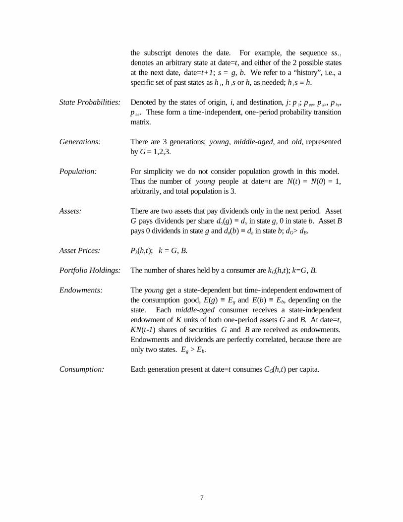
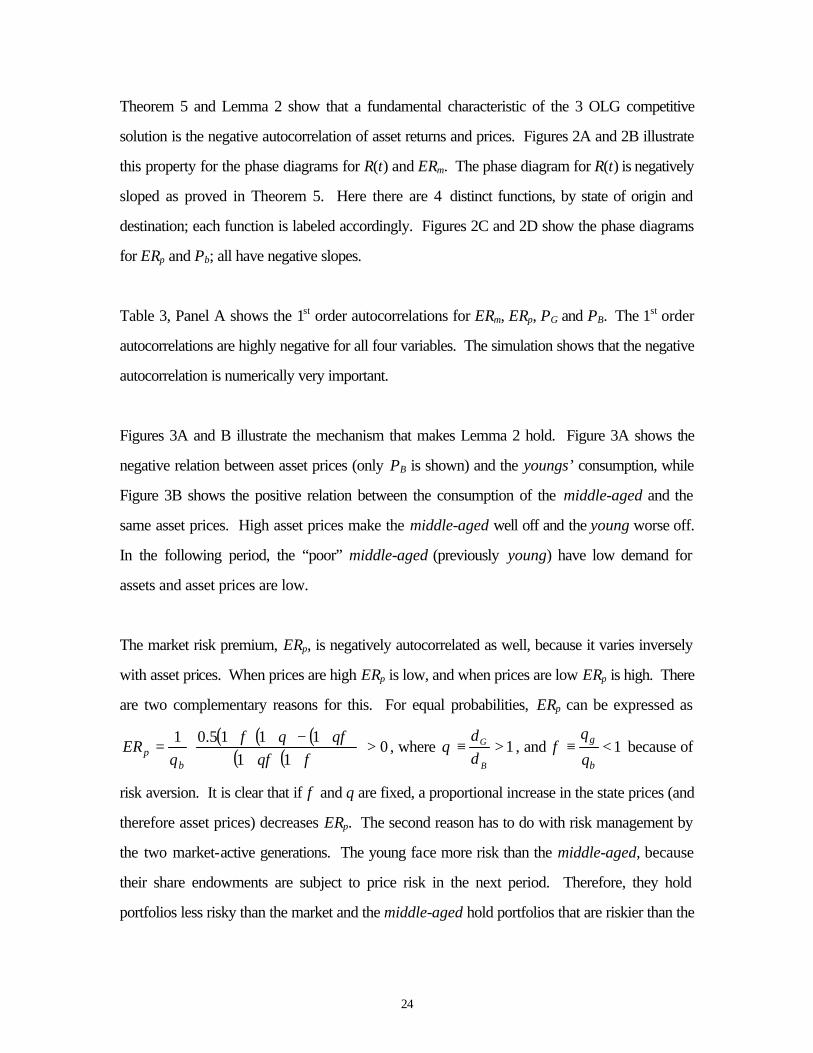
Theorem 5 and Lemma 2 show that a fundamental characteristic of the 3 OLG competitive
solution is the negative autocorrelation of asset returns and prices. Figures 2A and 2B illustrate
this property for the phase diagrams for R(t) and ERm. The phase diagram for R(t) is negatively
sloped as proved in Theorem 5. Here there are 4 distinct functions, by state of origin and
destination; each function is labeled accordingly. Figures 2C and 2D show the phase diagrams
for ERp and Pb; all have negative slopes.
Table 3, Panel A shows the 1st order autocorrelations for ERm, ERp, PG and PB. The 1st order
autocorrelations are highly negative for all four variables. The simulation shows that the negative
autocorrelation is numerically very important.
Figures 3A and B illustrate the mechanism that makes Lemma 2 hold. Figure 3A shows the
negative relation between asset prices (only PB is shown) and the youngs’ consumption, while
Figure 3B shows the positive relation between the consumption of the middle-aged and the
same asset prices. High asset prices make the middle-aged well off and the young worse off.
In the following period, the “poor” middle-aged (previously young) have low demand for
assets and asset prices are low.
The market risk premium, ERp, is negatively autocorrelated as well, because it varies inversely
with asset prices. When prices are high ERp is low, and when prices are low ERp is high. There
are two complementary reasons for this. For equal probabilities, ERp can be expressed as
( )( ) ( )( )( ) 0
111115.01
>
++
+−++=
φθφθφθφ
bp q
ER , where 1>≡B
G
dd
θ , and 1<≡b
g
q
qφ because of
risk aversion. It is clear that if φ and θ are fixed, a proportional increase in the state prices (and
therefore asset prices) decreases ERp. The second reason has to do with risk management by
the two market-active generations. The young face more risk than the middle-aged, because
their share endowments are subject to price risk in the next period. Therefore, they hold
portfolios less risky than the market and the middle-aged hold portfolios that are riskier than the

25
market.33 At low prices and a fixed risk premium, the young wish to increase their holdings
while keeping their portfolio composition the same. But this attempt by the young requires the
middle-aged to hold even riskier portfolios!34 The result in equilibrium is a higher price of risk.
This negative autocorrelation of returns, risk premia, and prices is a fundamental characteristic
of the 3-period OLG competitive model. It arises from the market interaction of agents, which
are ex-ante identical but whose wealth position differs because of their histories and their
horizons. In the next section we explore how this negative autocorrelation of returns might be
modified if transition probabilities are state-dependent.
V.3c. The Effect of Negative Underlying Probabilities on the Autocorrelation of Returns
We explore the effect of changing the autocorrelation structure of dividends on the
autocorrelation of expected returns and prices. Lemma 2 asserts that prices will be negatively
autocorrelated, without reference to the autocorrelation properties of dividends and
endowments. However, the magnitude of this negative autocorrelation may depend on the
dividend autocorrelation. In Table 3, Panels B and C we report two experiments, one with
positive and one with negative autocorrelation in the dividend process: πgg = πbb = 0.8, and πgg
= πbb = 0.2, respectively.
The autocorrelation of dividends has only a minor influence on the autocorrelation of prices and
returns. Positive autocorrelation of dividends makes ERm and ERp somewhat more negatively
autocorrelated, while negative autocorrelation of dividends makes it less negatively
autocorrelated. The negative autocorrelations of ERm and ERp are substantial in all three cases,
even though the dividend autocorrelation changes drastically. The reaction of prices is mixed.
PG is slightly less negatively autocorrelated while PB is substantially more negatively
autocorrelated when dividends are positively autocorrelated.
33 We found no counter-example in our simulations. 34 An example may be helpful: Let the young hold 1.0 share of the G-asset, while their portfolio composition is G1/B1 = 0.83 (a typical value). This implies that G2/B2 = 1.11. If the young buy 10% more shares and maintain their portfolio composition, the middle-aged would have to hold G2/B2 = 1.14.

26
The important conclusion from this experiment is that the substantial negative autocorrelations of
returns and prices that we found is driven by the workings of the market and not by the
structure of the fundamentals. The negative autocorrelation remains, regardless of the
autocorrelation of the fundamentals.
V.3d. The Correlation of Wealth with Aggregate Consumption
Table 4 shows the correlation of aggregate consumption as well as the consumption of each
generation with wealth.35 The 1st column shows that aggregate consumption has a low
correlation with wealth. The succeeding columns show the reason for this low correlation: the
correlation of consumption with wealth varies by generation. This result stands in sharp contrast
with our benchmark models, where aggregate consumption is perfectly correlated with wealth.
The low correlation between wealth and aggregate consumption is generated by the negative
autocorrelation of asset prices and thus wealth. High asset prices today imply high consumption
for the middle-aged but low consumption for the young who have to acquire the high-priced
assets. The old are not affected by the current market conditions; but because of the negative
correlation, prices were likely to have been low when they were middle-aged, which implies
low consumption for them now.
VI. CONCLUSION
The contribution of this paper is to show that in a 3-generation OLG competitive equilibrium,
expected market returns, risk premia, and asset prices are negatively autocorrelated, regardless
of the autocorrelation structure of the fundamentals. Market interactions between identical
consumers, except for their age, gives rise to complex price and return dynamics even when
dividends, endowments, and aggregate consumption are i.i.d. This result is qualitatively
35 In this model, all variation in wealth is related to prices and it is transitory, because the quantities of the asset are fixed.

27
consistent with empirical observation, and it stands in sharp contrast to the results of the
standard paradigm --the infinite-lived representative consumer model-- in which return and
price dynamics closely mirror the dynamics of the dividends, and prices and expected returns
are not autocorrelated when the fundamentals are not. The 3-generation OLG model provides
a simple and intuitive explanation of the long-run negative autocorrelation of returns. A
byproduct of this negative autocorrelation is that the correlation between aggregate consumption
and wealth is low.
In our model, the young receive a consumption endowment while the middle-aged receive
assets that pay risky dividends in the following period. We assume away market frictions,
incomplete markets, asymmetric information and all types of irrationality.
We show that negative autocorrelation in expected returns, risk premia, and prices (and the
resulting “excess” and time-varying volatility) is a fundamental property of the model, because
consumers’ excess supply for assets is price-elastic. The middle-aged can choose how much
of their asset endowment to sell, because they have an alternative use: to hold the assets over to
the next period and consume the dividends. The excess supply of the middle-aged depends on
the quantity of assets they purchase when young, which in turns depends on the prices they
encountered at that time. In this way, the history of each generation affects the date=t
equilibrium, even though the distributions of endowments and dividends do not change over
time.
Price-elastic excess supply of assets is a feature of everyday markets. It is perhaps surprising
that including this feature in an OLG model generates return and asset price properties at such
great variance with our usual concept of efficient market equilibrium. Yet, the properties of our
model are qualitatively similar to those in the data. We conclude that the observed predictability
of returns are difficult to explain because our ideas of market efficiency are informed mainly by
the properties of representative consumer models, which do not capture the effects of
intergenerational trading.

28
Assuming a 3-period lifespan necessarily confines the analysis to long-run behavior. To address
short-run properties of asset returns, the number of periods consumers live must be increased.
The interaction of many generations each with a slightly different financial history will
undoubtedly produce much richer dynamics. Such an extension presents a serious technical
challenge and is the subject of ongoing research.

29
VII. REFERENCES Abel, Andrew B., 1990, Asset prices under habit formation and catching up with the Jones’,
American Economic Review 80, 38-42. Azariadis, Costas, 1993, Intertemporal Macroeconomics, Oxford: Blackwell Publishers. Azariadis, Costas, James Bullard, and Lee Ohanian, 2002, Trend-reverting fluctuations in the
life-cycle model, Journal of Economic Theory, (forthcoming). Campbell, John Y., 2001, Consumption-based asset pricing, manuscript prepared for George
Constantinides, Milton Harris, René Stulz, eds.: Handbook of Economics and Finance 1 (Elsevier Science, Amsterdam).
Balasko, Yves, David Cass, and Karl Shell, 1980, Existence of competitive equilibrium in a general overlapping-generations model, Journal of Economic Theory 23, 3, 307-322.
Benninga, Simon, Aris Protopapadakis, 1991, Stock market premia, market completeness, and relative risk aversion, American Economic Review 25, 1, 49-58.
Campbell, John Y., John H. Cochrane, 1999, By force of habit: A consumption-based explanation of aggregate stock market behavior, Journal of Political Economy 107, 205-251.URL
Campbell, John Y., Robert J. Shiller, 1988, Stock prices, earnings, and expected dividends, The Journal of Finance. 43, 661-676. URL
Campbell, John Y., Robert J. Shiller, 1998, Valuation ratios and the long-run stock market outlook, Journal of Portfolio Management 24, 11-26.
Cecchetti, Stephen G., Pok-Sang Lam, Nelson C. Mark, 1990, Mean reversion in equilibrium asset prices, The American Economic Review 80, 398-418. URL
Cecchetti, Stephen G., Pok-Sang Lam, Nelson C. Mark, 1993, The equity premium and the risk free rate: Matching the moments, Journal of Monetary Economics 31, 21-45. URL
Chattopadhyay, Subir, Piero Gottardi, 1999, Stochastic OLG models, market structure, and optimality, Journal of Economic Theory 89, 21-67.
Cochrane, John H., 1991, A simple test of consumption insurance, Journal of Political Economy 99, 957-976. URL
Cochrane, John H., 2001, Asset Pricing, Princeton University Press, Princeton New Jersey. Constantinides, George M., 1990, Habit formation: A resolution to the equity premium puzzle,
Journal of Political Economy 98, 519-543 Constantinides, George M., and Darrell Duffie, 1996, Asset Pricing with Heterogeneous
Consumers, Journal of Political Economy 104, 219-240. URL Constandinides, George, John B. Donaldson, Rajnish Mehra, 2002 Junior can’t borrow: a new
perspective on the equity premium puzzle, Quarterly Journal of Economics 117, 269-296
Daniel, Kent 2003 The power and size of mean reversion tests, Kellogg School of Management Working Paper.
Fama, Eugene F., Kenneth R. French, 1988, Permanent and temporary components of stock prices, Journal of Political Economy 96, 246-273. URL

30
Fama, Eugene F., Kenneth R. French, 2001, The equity premium, The Center for Research in Security Prices Working Paper No. 522. URL
Jegadeesh, Narasimham, and Sheridan Titman, 1993, Returns to buying winnings and selling losers: Implications for stock market efficiency, Journal of Finance 48, 65-91. URL
Kandel, Shmuel, and Robert F. Stambaugh, 1991, Asset returns and intertemporal preferences, Journal of Monetary Economics 27, 39-71.
Le Roy, Stephen F., and Richard Porter, 1981, The present value relation: Tests based on variance bounds, Econometrica 49, 555-557.
Lettau, Martin, and Sydney Ludvigson, 2001, Consumption, aggregate wealth, and expected stock returns, Journal of Finance 56, 815-49.
Lettau, Martin, and Sydney Ludvigson, 2004, Understanding Trend and Cycle in Asset Values: Reevaluating the Wealth Effect on Consumption, American Economic Review 94, 1.
Lewellen, Johnathan, 2002, Momentum and autocorrelation in stock returns, Review of Financial Studies 15, 533-563.
Lo, Andrew W. , A. Craig MacKinlay, 1988, Stock market prices do not follow random walks: Evidence from a simple specification test, The Review of Financial Studies, 41-66.URL
McCandless, George Jr., T., Wallace, Neil, 1991, Introduction to Dynamic Macroeconomic Theory, Harvard University Press, Cambridge Massachusetts.
Poterba, James M., 2001, Demographic structure and asset returns, Review of Economics and Statistics 83, 565-584.
Poterba, James M.; Lawrence H. Summers, 1988, Mean Reversion in Stock Prices, Journal of Financial Economics 22, 27-59.
Samuelson, Paul A., 1958, An Exact Consumption-Loan Model of Interest with or without the Social Contrivance of Money, Journal of Political Economy 66, 467-482.
Shilller, Robert, J., 1981, Do stock prices move too much to be justified by subsequent changes in dividends?, American Economic Review 71, 421-436.
Summers, Lawrence H., 1986, Does the stock market rationally reflect fundamental values? Journal of Finance 41, 591-601.

31
APPENDIX 1: THE INDIVIDUAL CONSUMER’S OPTIMIZATION PROBLEM A state-by-state rewriting of the individual maximization problem in Langrangian form yields (s is the state of birth), (A1.1)
( ) ( )[ ] ( )[ ]∑ ∑∑= ==
++
bgl bgmlm
bglslt
slmCslBslGlC
sBsGC
slmCUslCUsCUhshZE, ,
3,
2212+1+
)()(),(),(s
)(),( (s)
][=)},1({ Max
32
2211
1πδπδ
(A1.2a) ( ) ( ) ( ) ( ) ( ) ( ) ( )s- 1 11111 EsBshpsGshpsCs BG −− ++− λ ,
(A1.2b) ( ) ( ) ( ) ( ) ( ) ( ) ( ) ( )[ ] ( ) ( )[ ]{ }slBKlpslGKlpsBldsGldslCsl BGBG 22112 - -- - 2 −−− λ , (A1.2c) ( ) ( ) ( ) ( ){ }slBmdslGmdslmCslm BG 223 )()( - 3 −− λ ; s,l,m = g,b. First Order Conditions The FOCs from differentiating w.r.t. young, middle-aged and old consumptions yield,
( )[ ] ( )ssCU 11' λ= , ( )[ ]{ } ( )sggsggCUggsg 33
'2 λπδπ = ,
( )[ ] ( )sgsgCUsg 22' λδπ = , ( )[ ]{ } ( )sgbsgbCUgbsg 33
'2 λπδπ = ,
( )[ ] ( )sbsbCUsb 22' λδπ = , ( )[ ]{ } ( )sbgsbgCUbgsb 33
'2 λπδπ = ,
( )[ ]{ } ( )sbbsbbCUbbsb 33'2 λπδπ = .
where,
(A1.3a,b) ( )( )
( )[ ]( )[ ]
==sCUsgCU
ssg
q sghg1
2
''
12
δπλ
λ,
( )( )
( )[ ]( )[ ]
==sCUsbCU
ssb
q sbhb1
2
''
12
δπλ
λ,
(A1.3c,d) ( )( )
( )[ ]( )[ ]
==sgCU
sggCUsgsgg
q gghgg2
3
''
23
δπλλ
, ( )( )
( )[ ]( )[ ]
==sgCUsgbCU
sgsgb
q gbhgb2
3
''
23
δπλλ
,
(A1.3e,f) ( )( )
( )[ ]( )[ ]
==sbCU
sbgCUsbsgb
q bghbg2
3
''
23
δπλλ
, ( )( )
( )[ ]( )[ ]
==sbCU
sbbCUsb
sbbq bbhbb
2
3
''
23
δπλλ
,
are the individual’s probability-weighted discounted one-period marginal rates of substitution, which the individual equates to the economy-wide state prices:
1+hsq in youth and 21 ++ shsq in middle age. Differentiating
with respect to share holdings of each asset to the young k(1,h), k={α,β}, yields,
(A1.4) ( ) ( )( )
( )( )
)(12
+)(12
= bdssb
gdssg
hp kkk λλ
λλ
.

32
Similarly, differentiating with respect to the share holdings of the middle-aged k2(sg) and k2(sb) yields:
(A1.5a) ( ) ( )( )
( ) ( )( )
( )bdsgsgb
gdsg
sgghgp kkk 2
3+
23
= λλ
λλ
,
(A1.5b) ( ) ( )( )
( ) ( )( )
( )bdsbsbb
gdsb
sbghbp kkk 2
3+
23
= λλ
λλ
.
Since each person equalizes her personal marginal rate of substitution to the state prices, these equations become pricing equations:
(A1.6)
( ) ( ) ( )( ) ( ) ( )( ) ( ) ( ). + =
, + =
, + =
bdqgdqhbp
bdqgdqhgp
bdqgdqhp
khbbkhbgk
khgbkhggk
khbkhgk
These equations merely show that share prices are the present value of the dividends. Finally, differentiating with respect to the Langrangian multipliers we get back the 7 budget constraints. (A1.7a) ( ) ( ) ( ) ( ) ( ) ( )sBhpsGhpEsC BG 111 - s −= , (A1.7b) ( ) ( ) ( ) ( )[ ] ( ) ( )[ ]sgBKhgpsgGKhgpsGdsgC BGG 2212 (g) −+−+= , (A1.7c) ( ) ( ) ( )[ ] ( ) ( )[ ]sbBKhbpsbGKhbpsBbdsbC BGB 2212 )()( −+−+= , (A1.7d,e) ( ) ( )sgGgdsggC G 23 )( = , ( ) ( )sgBbdsgbC B 23 )( = , (A1.7f,g) ( ) ( )sbGgdsbgC G 23 )( = , ( ) ( )sbBbdsbbC B 23 )( = . A a “young” consumer takes as given the 14 asset prices that she may encounter over her lifetime and solves her optimal lifetime consumption and asset holding plan. Seven consumptions –C1(s), C2(sg), C2(sb), C3(sgg), C3(sgb), C3(sbg), C3(sbb)-- and six asset holdings –G1(s), G2(sg), G2(sb), B1(s), B2(sg), B2(sb). That gives 13 variables to solve for, and there are 6 MRS equations and 7 budget constraints. In addition, we get 6 pricing equations. Another way to summarize the budget constraints is to express them in terms of one intertemporal budget constraint: (A1.8)
( ) ( )[ ] ( ) ( )[ ]( ) ( ) ( ) ( ) ( )[ ] ( ) ( )[ ]sbbCqsbgCqqsgbCqsggCqqsbCqsgCqsC
KhbphbpqKhgphgpqE
hbbhbghbhgbhgghghbhg
BGhbBGhgs
3333221 ++++++=
++++

33
APPENDIX 2: SOLUTIONS FOR THE BENCHMARK MODELS Appendix 2A: The ILRC (Representative Consumer) Model The equilibrium solution is immediate in this case, because the representative consumer consumes all that is available in each period, and thus has no meaningful decision to make. The state prices reflect total available endowment, and the asset prices are shadow prices that reflect the equality of latent excess demand and supply. The equilibrium consumption is given by, ( ) ss KdEsC += . This is enough to compute the state prices and the shadow prices of the assets.
(A2.1a,b) gGg
Gggggg KdE
KdEq πδπδ
γ
=
+
+= , γ
γ
πδπδ ?KdE
KdEq b
Bb
Gggbgb =
+
+= ,
(A2.1c,d) bBb
Bbbbbb KdE
KdEq πδπδ
γ
=
++
= , γ
γ
πδπδ −=
++
= ?KdEKdE
q gGg
Bbbgbg ,
where, 1>+
+=
bb
gg
KdE
KdE? , and probabilities are state-independent.
Asset prices then are: (A2.2a) ( ) GgGggG ddqgP πδ== , ( ) GgGbgG d?dqbP γπδ −== ,
(A2.2b) ( ) BbBbbB ddqbP πδ== , ( ) BbBgbB d?dqgP γπδ== .
Appendix 2B: The 2-OLG Competitive Model The appropriate transformation of the 3-period OLG model to a 2-period one is as follows: All parameters stay the same. The young still receive E(s) endowments and the old (rather than the middle-aged) receive K units of each of the two risky 1-period assets. Since these assets do not produce dividends until the following period, the old must sell them to their only costumer, the young. The young buy these assets with some of their endowment income. The old consume both the dividends of the assets they bring into the period and the proceeds from the sale of their endowment of assets. This model is strictly recursive, i.e., past history doesn’t matter, so that there is a single solution for a good state and another one for a bad state. The reason follows.

34
For simplicity, assume that bsbgsg ππππ == , . Consider the good (g) states at dates t and
t+n. At both dates the supply of the consumption good is ( ) GKdgE + . At both dates, the young are endowed with E(g), the old are endowed with K, and the young purchase all the assets of the old. Thus, the past has no impact on the demand and supply of the present state. The solution at both dates must be the same. The same argument applies identically to bad states.36 Thus, consumption is not indexed by date or history. We solve the problem by first solving the individual consumer’s maximization problem. Then we impose the asset market clearing condition. Consider the individual’s lifetime maximization problem:
(A2.3) ( ){ } ( )[ ] ( )[ ]{ }
.
, E+ ,E Max 1+2t11t
)(),(G)(sC),(C
211+21
sCUsCUssZsBs
sδ=+
subject to the age=1, 2, budget constraints, respectively: (A2.4a) ( ) ( ) ( ) ( ) ( ) ( )sBPsGPsEsC BG 111 s-s- = , (A2.4b) ( ) ( ) ( ) ( ) ( ) ( ) ( )KsPKsPsdsBsdsGsC BGBG 11111112 +++++ +++= . The derivation of the first order conditions follows. At any date=t, the young and old jointly determine equilibrium allocations. The young equate their expected marginal rates of substitution to the market’s, and the old do not have a relevant marginal rate of substitution. (A2.5a)
( ) ( ) ( )( ) ( )
( ){ } ( )[ ] ( )[ ] ( )[ ]{ }bCUgCUsCUssWEMax bgt
sbCsgCsBsGsC 2211
,,,
,22
111
ππδ ++=+
,
(A2.5b) ( ) ( ) ( ) ( ) ( ) ( ){ }sBsPsGsPsCsE BG 111 - - )(s1 −− λ , (A2.5c) ( ){ }KgPKgPgdsGgCg BGG )(-)( )( - )()(2 12 −− λ , (A2.5d) ( ){ }KbPKbPbdsBbCb BGB )(-)( -)(- )()(2 12λ− . Since dG(b) = dB(g) = 0, the associated terms have been deleted from the equations above. First Order Conditions: The FOCs from differentiating w.r.t. young, middle-aged and old consumptions yield,
36 If the transition probabilities depend on the immediate predecessor state, then there will be four rather than two equilibria, one each for states gg, gb, bg, and bb.

35
(A2.6) ( ) ( )ssC 11 λγ =− , ( ) ( )ggCg 22 λδπ γ =− , ( ) ( )bbCb 22 λδπ γ =− .
Where the young consumers’ probability-weighted discounted one-period marginal rates of substitution is equated to the economy-wide state prices: sgsg qq , ,
(A2.7a,b) γ
πδλλ
==
)()(
)(1)(2
2
1
gCsC
sg
q gsg , γ
πδλλ
==
)()(
)(1)(2
2
1
bCsC
sb
q bsb ,
Differentiating with respect to share holdings of each asset to the young k1(h), k={α,β}, yields the general relation,
(A2.8) ( ) ( )bdsb
gdsg
sP kkk )(1)(2
+)(1)(2
= )(λλ
λλ
.
Since each person equalizes her personal marginal rate of substitution to the state prices, these equations become pricing equations: (A2.9) ( ) ( )bdqgdqsP ksbksgk + =)( .
Under our payoff structure this yields: (A2.10a,b) ( )gdqgP GggG =)( , ( )gdqbP GbgG =)( ,
(A2.10c,d) ( )bdqgP BgbB =)( , ( )bdqbP BbbB =)( .
The asset market clearing condition is that at the end of date=t all shares outstanding are held by the young, (A2.11) ( ) ( ) KsBsG == 11 . The simplest approach is to impose the asset market clearing condition directly to equations (A2.1). This gives, (A2.12a) ( ) ( ) ( ) ( )KgPKgPgEgC BG -- = 1 , (A2.12b) ( ) ( ) ( ) ( )KbPKbPbEbC BG -- = 1 , (A2.12c) ( ) ( ) ( )KgPKgPKdgC BGG ++=2 , (A2.12d) ( ) ( ) ( )KbPKbPKdbC BGB ++=2 . Substitute out the asset prices to get,

36
(A2.13a) ( ) ( ) [ ]BgbGgg dqdqKgEgC +- = 1 ,
(A2.13b) ( ) ( ) [ ]BbbGbg dqdqKbEbC +- = 1 ,
(A2.13c) ( ) [ ]BgbGggG dqdqKKdgC ++=2 ,
(A2.13d) ( ) [ ]BbbGbgB dqdqKKdbC ++=2 .
Now substitute the consumptions into the state prices to get,
(A2.14a) ( ) ( ) ( )( )
( )( )
+
BbGg d
bCgC
FdgCgC
FKgEgCγγ
2
1
2
11 - = ,
(A2.14b) ( ) ( ) ( )( )
( )( )
+
BbGg d
bCbC
FdgCbC
FKbEbCγγ
2
1
2
11 - = ,
(A2.14c) ( ) ( )( )
( )( )
+
+= BbGgG d
bCgC
FdgCgC
FKKdgCγγ
2
1
2
12 ,
(A2.14d) ( ) ( )( )
( )( )
+
+= BbGgB d
bCbC
FdgCbC
FKKdbCγγ
2
1
2
12 ,
where bbgg FF πδδπ ≡≡ ; are constants.
These equations have to be solved simultaneously. As in the 3-OLG case, the individual’s budget constraint cannot be reduced to the economy-wide resource constraint used by the social planner. Thus the competitive solution, though stationary, is not the SP solution. Appendix 2C: The 3-OLG Social Planner Model The social planner (SP) solves the following maximization problem that includes arbitrary weights across individuals and generations.
(A2.15) ( )[ ] ( )[ ] ( )[ ]∑ ∑
Θ+Θ+Θ −−−t
hhthhth
hht hCUhCUhCUMax 32
,1,32,1,21,1,1 δπδππ
s.t., ( ) ( ) ( ) ( ) ( )∑+=++k
k sdKsEsCsCsC 321 ,
There is no economic connection between successive time periods, because consumption allocations at date=t cannot affect consumption allocations at date=t+1 or beyond. Thus, the

37
SP has to make only 2 allocations, for s = g, b. To simplify the algebra, we also assume that, .,;1 tGG,t ∀=Θ
Normalize the problem and introduce some notation simplifications,
(A2.16) ( )[ ] ( )[ ] ( )[ ]sCUsCUsCUMax ssssss 32
,12,11,1 δπδππ −−− ++ ,
s.t., ( ) ( ) ( ) ( ) ( )sKdsEsCsCsC k+=++ 321 , for s=g,b. We drop the summation sign for the dividends, because we assume all along an orthogonal payout scheme. The first order conditions, in addition to the resource constraint are as follows: (A2.17) ( )[ ] 01
',1 =−− λπ sCUss , ( )[ ] 02
',1 =−− λπ sCUss , ( )[ ] 03
',1 =−− λπ sCUss .
These conditions simplify to the following: (A2.18) ( )[ ] ( )[ ] ( )[ ]sCUsCUsCU ssssss 3
'2,12
',11
',1 δπδππ −−− == .
Substituting in the RRA utility function and canceling out the probabilities we get,
γγγ δδ −−− == 32
21 CCC , which simplifies to, 3
2
2
1
1 CCC γγ δδ−−
== , dropping the index s, with the understanding that there are two solutions (s=g, b). The rule that the SP divides available consumption is given by,
(A2.19a) kKdEC +=
++ γγ δδ
21
1 1 , γγ δδ
211
1 ++
+= kKdE
C ,
(A2.19b) γδ1
23 CC = , γδ1
12 CC = . There are 4 “shadow” state prices in this economy, and they are as follows: (A2.20a,b)
( )( )
( )( )
γγ
δπδπ−−
=
=
gCgC
gCgC
q gggggg2
3
1
2 , ( )( )
( )( )
γγ
δπδπ−−
=
=
gCbC
gCbC
q gbgbgb2
3
1
2 ,
(A2.20c,d)
( )( )
( )( )
γγ
δπδπ−−
=
=
bCgC
bCgC
q bgbgbg2
3
1
2 , ( )( )
( )( )
γγ
δπδπ−−
=
=
bCbC
bCbC
q bbbbbb2
3
1
2 .

38
The consumption ratios are, For the g to g, and b to b transitions, there is one ratio,
( )( )
( )( )
( )( )
( )( )
γδ1
2
3
1
2
2
3
1
2 ====bCbC
bCbC
gCgC
gCgC
, while for the g to b and b to g transitions there is
another. Note that,
(A2.21) ( )( ) 1
1
1 >=+
+= ?
KdE
KdE
bCgC
bb
gg .
Therefore,
(A2.22) ( )( )
γδ1
1
2 ?bCgC
= , and ( )( )
γδ1
1
1
2 −= ?gCbC
.
Substitute these relations to solve for the state prices:
ggggq π= , bbbbq π= , γπ ?q gbgb = , γπ −= ?q bgbg . Asset prices then are:
(A2.23a,b) ( ) GggGggG ddqgP π== , ( ) GbgGbgG d?dqbP γπ −== ,
(A2.23c,d) ( ) BbbBbbB ddqbP π== , ( ) BgbBgbB d?dqgP γπ== .

39
APPENDIX 3: PROOF THAT THE SOCIAL PLANNER SOLUTION IS NOT FEASIBLE IN A COMPETITIVE EQUILIBRIUM.
Theorem 1: The social planner solution is not attainable in a competitive market. Proof: The social planner solves the equilibrium problem constrained by available resources (equation 12): (12) ( ) ( ) ( ) ( ) ( )∑+=++
kk sdKsEsCsCsC 321 .
It produces a recursive solution in which the consumption of all 3 generations depends only on the current state. In contrast, the competitive equilibrium has an additional constraint, the wealth constraint of each individual consumer. This can be expressed as:
(A3.1)
( ) ( ) ( ) ( )
( ).,,
,,
, ,213,,,
, ,12,1
,1,
1 2
121
1
1
1
∑ ∑
∑ ∑∑
= =++
=+
=+
+ +
+++
+
+
+
+
+=+
bgs bgssssss
BGk bgss
bgskss
sssCqq
ssCqsCKssPqsE
It is clear by inspection that these two constraints are not equal, since (A3.1) contains future state-dependent consumptions that are not relevant to the social planner. Thus, the social planner solution will not satisfy (A3.1) There are two present value constraints, for states g and b. We substitute into the constraint the social planner solution and ask whether the present value constraint is identical to the resource constraint. The constraints for the two possible states are: (A3.2.a)
( ) ( ) ( )[ ] ( ) ( )[ ] ( ) ( )
( ) ( )[ ] ( ) ( )[ ].)(
3333
221
bCqgCqqbCqgCqq
bCqgCqgCKbPbPqKgPgPqgE
bbbggbgbgggg
gbggBGgbBGgg
++++
++=++++
(A3.2.b)
( ) ( ) ( )[ ] ( ) ( )[ ] ( ) ( )
( ) ( )[ ] ( ) ( )[ ].)(
3333
221
bCqgCqqbCqgCqq
bCqgCqbCKbPbPqKgPgPqbE
bbbgbbgbggbg
bbbgBGbbBGbg
++++
++=++++.
The state prices are from equations (6) and the asset prices are from equations (11). (17) gggq π= , bbbq π= , γπ −= Fq bgb , γπ Fq gbg = .

40
(A3.3) ( ) GggG dqgP = , which reduces to, ( ) GggG dgP π= ,
( ) GbgG dqbP = , which reduces to, ( ) GbgG dFbP γπ= ,
( ) BbbB dqbP = , which reduces to, ( ) BbbB dbP π= ,
( ) BgbB dqgP = , which reduces to, ( ) BgbB dFgP γπ −= .
Substitute all this into equations (A3.2a&b) and collect terms to get,
(A3.4a)
( ) [ ] [ ]( ) ( )
( ) ( )[ ] ( ) ( )[ ].)(
3333
221
bCgCFFbCFgC
bCFgCgC
KddFFKdFdgE
bgbbgg
bg
BbGgbBbGgg
ππππππ
ππ
ππππππ
γγγ
γ
γγγ
++++
++=
++++
−−
−
−−
(A3.4b)
( ) [ ] [ ]( ) ( )
( ) ( )[ ] ( ) ( )[ ].)(
3333
221
bCgCFbCFgCF
bCgCFbC
KddFKdFdFbE
bgbbgg
bg
BbGgbBbGgg
ππππππ
ππ
ππππππ
γγγ
γ
γγγ
++++
++=
++++
−
−
collect terms further to get:
(A3.5a) ( ) ( ) ( ){ }
( ) ( ) ( ) ( ).)( 33221
22
bCFgCbCFgCgC
dFFdKgE
bgbg
BbbgGbgg
γγ
γγ
ππππ
ππππππ−−
−−
++++=
++++
(A3.5b) ( ) ( ) ( ){ }
( ) ( ) ( ) ( ).)( 33221
22
bCgCFbCgCFbC
ddFFKbE
bgbg
BbbgGbgg
ππππ
ππππππγγ
γγ
++++=
++++
(A3.6a) ( ) { }
( ) ( ) ( ) ( ) .)(2
1
2
1
1
1
1
11γγγγγγ
γ
δπδπδπδπ
ππ
bCFgCbCFgCgC
dFdKgE
bgbg
BbGg
−−
−
++++
=++
(A3.6b) ( ) { }
( ) ( ) ( ) ( ) .)(2
1
2
1
1
1
1
11γγγγγγ
γ
δπδπδπδπ
ππ
bCgCFbCgCFbC
ddFKbE
bgbg
BbGg
++++
=++
(A3.7a) ( ) { }
).(1)(1 1
11
1
21bCFgC
dFdKgE
bgg
BbGg
++
++
=++
−
−
γγγγγ
γ
δδπδπδπ
ππ

41
(A3.7b) ( ) { }
).(1)(1 1
11
1
21gCFbC
ddFKbE
gbb
BbGg
++
++
=++
γγγγγ
γ
δδπδπδπ
ππ
(A3.8a)
( ) { }
( )( ) ( )( ).111121
BbGgg
BbGg
KdbEFKdgE
dFdKgE
+
+Γ++
++Γ
=++
−
−
γγγγγ
γ
δδπδπδπ
ππ
(A3.8b)
( ) { }( )( ) ( )( ).11
1121
GgBbb
BbGg
KdgEFKdbE
ddFKbE
+
+Γ++
++Γ
=++
γγγγγ
γ
δδπδπδπ
ππ
where, 121
1−
++≡Γ γγ δδ .
Now write the resource constraint for state s = g, b, from equation (8 of the text) above, (A3.9) ( ) ( ) ( ) ( )sCsCsCKdsE s 321 ++=+ .
This becomes,
(A3.10) ( ) ( ) ( ) ( ) γγ δδ2
1
1
11 sCsCsCKdsE s ++=+ ,
(A3.11) ( ) ( ) 11
−Γ=+ sCKdsE s .
It is clear that the present value constraints (equations A3.8a & b) are not identical to the resource constraint (equation A3.11). In particular, in order for the two constraints to coincide, the following conditions must be met. (A3.12.a) BBbGg ddFd =+ −γππ ,
(A3.12.b) BBbGg dddF =+ ππ γ ,
(A3.13) γγ δδπ11
11 +=
+s ,

42
(A3.14) ( ) 0111
1 =
+ γγγ δδπ FsC s ,
These conditions are fulfilled only when there is no uncertainty, i.e., πg = 1.0, πb = 0.0, and by definition Φ = 1; in this case only (A3.12.a), (A3.13), and (A3.14) apply. Therefore, it is clear that the social planner solution is not attainable, in general, in a competitive market. An implication of the above result is that there is no other competitive market solution of this class, i.e., consumption outcomes that depend only on the current state of the world. This is because the competitive market solution has to obey the individuals’ wealth constraint, in addition to the other 1st order conditions that the S.P. solution obeys. As we show above these wealth constraints are not redundant, thus the model is overidentified for this class of solutions and there is no solution.
Q.E.D.

43
APPENDIX 4: PROOF THAT THE COMPETITIVE SOLUTION IS APERIODIC
Theorem 2: The competitive solution in this economy is path-dependent, even though all good and bad states have path-independent resource allocations. Proof: Start with the following 3-period periodic equilibrium. C1(g), C1(b), C2(gg), C2(gb), C2(bg), C2(bb), C3(ggg), C3(ggb), C3(gbg), C3(gbb), C3(bgg), C3(bgb), C3(bbg), C3(gbb). The equilibrium is one in which each of the 8 possible life paths has its own consumption experience, and that past history is not relevant. We show that this equilibrium collapses to the social planner equilibrium, which we have already shown is not feasible in the competitive economy. The equalization of the marginal rates of substitution implies the following equalities:
(A4.1a) ( )( )
( )( )gggC
ggCggCgC
3
2
2
1 = , (A4.1b) ( )( )
( )( )ggbC
ggCgbCgC
3
2
2
1 = ,
(A4.1c) ( )
( )( )
( )gbgCgbC
bgCbC
3
2
2
1 = , (A4.1d) ( )( )
( )( )gbbC
gbCbbCbC
3
2
2
1 = ,
(A4.1e) ( )( )
( )( )bggC
bgCggCgC
3
2
2
1 = , (A4.1f) ( )( )
( )( )bgbC
bgCgbCgC
3
2
2
1 = ,
(A4.1g) ( )
( )( )
( )bbgCbbC
bgCbC
3
2
2
1 = , (A4.1h) ( )( )
( )( )bbbC
bbCbbCbC
3
2
2
1 = .
These equalities are derived as follows: imagine being in state g whose parent state is also g. The young equalize their marginal rates of substitution (MRS) between their current and future consumptions, e.g., ( )gC1 , and ( )ggC2 and ( )gbC2 , while the middle-aged equalize to the same MRS ( )ggC2 , and ( )gggC3 and ( )ggbC3 . Do this until all the possible combinations are exhausted. The economy-wide resource constraints for the g and b states are, (A4.2a) ( ) ( ) ( )gggCggCgCKdG 321 ++= , (A4.2b) ( ) ( ) ( )bggCggCgCKdG 321 ++= , (A4.2c) ( ) ( ) ( )gbgCbgCgCKdG 321 ++= , (A4.2d) ( ) ( ) ( )bbgCbgCgCKdG 321 ++= , (A4.2e) ( ) ( ) ( )ggbCgbCbCKdB 321 ++= , (A4.2f) ( ) ( ) ( )bgbCgbCbCKdB 321 ++= , (A4.2g) ( ) ( ) ( )gbbCbbCbCKdB 321 ++= ,

44
(A4.2h) ( ) ( ) ( )bbbCbbCbCKdB 321 ++= . Equations (A4.2) imply the following equalities: (A4.3) ( ) ( ) ( )ggCbggCgggC 333 ≡= , ( ) ( ) ( )bgCbbgCgbgC 333 ≡= ,
( ) ( ) ( )gbCbgbCggbC 333 ≡= , ( ) ( ) ( )bbCbbbCgbbC 333 ≡= . These equalities substituted into the corresponding equations (A4.1) provide the following additional equalities: (A4.4) ( ) ( ) ( )gCbgCggC 222 ≡= , ( ) ( ) ( )bCbbCgbC 222 ≡= . Going back once more to the resource constraints (equations A.5.2) we see that, (A4.5) ( ) ( ) ( )gCbgCggC 333 ≡= , ( ) ( ) ( )bCbbCgbC 333 ≡= . This proves that this particular periodicity collapses to an equilibrium that depends only on the current state of the economy. Q.E.D. The obvious question is: what if we expand the recursion to 4 periods or more. In order to do that we must index consumptions by the parent state (or states). Write the consumption of a young consumer born in state=g, with a parent state=g as ( )ggC ;1 . It is important to realize that this implies ( )gggC ;2 , ( )ggbC ;2 , ( )ggggC ;3 , ( )gggbC ;3 ,
( )ggbgC ;3 , ( )ggbbC ;3 . In other words, for such a recursion to make sense, it must be that all the subsequent consumptions also have to be indexed by the same pre-birth parent state. It is clear from this observation that the above proof carries through for any periodicity. This is because the number of equations (MRS equalities and resource constraints) will expand proportionally to the number of states consumptions are indexed by. For example, a 4-period periodicity implies twice as many equations as a 3-period periodicity etc. Thus, the same method of searching for old-aged consumption equalities, substituting them back into the resource constraints and repeating the cycle applies, and produces the same result. Thus, periodicity of any finite length collapse to an equilibrium that depends only on the current state. By Theorem 1 a solution that depends only on the current state of the economy cannot be a competitive market equilibrium. Thus, the competitive market equilibrium cannot be periodic.

45
APPENDIX 5: DERIVATION OF THE DIFFERENCE EQUATIONS: The solution reduces the problem to solving for the shares held by successive middle-aged cohorts into each date=t along all possible state histories, hT. We develop two sets of equations. The first is a recursive relation for R(h-1) that incorporates the first order conditions over successive states. The second is an implicit recursive relation for asset holdings that the middle age bring into the state, G1(h-1) or B1(h-1), which are compatible with first order and the asset market clearing conditions. Numbering Convention: To develop the equations we need a numbering convention that can reference every state on the tree. On a tree of length T there are 2T+1-1 states. There is also a special initial state before the start of the world at date=0. The individual states are numbered consecutively, starting from the top of the tree each period. There are 2t states at each date. The initial state is state i=0, the state at t=0 is i=1, the states at t=1 are i=2-3, states at t=2 are i=4-7, and so fourth. From date=0 to date=T including the initial state, the current state s is indexed by i= 0,1,…, 2T+1-1. By convention, an odd state is a “bad” state and an even state is a “good” state. The successor states of a particular parent state, s=i, are states s=2i (sg) and s=2i+1 (sb). Similarly, the parent state is Integer(i/2). The Difference Equations: We derive first the recursive relation for R(i). We will only illustrate the derivation for transitions into good states, noting that the expression for bad states has an identical form. From a particular parent i write the definition for R(i),
(A5.1a) ( ) ( )( )
( ) ( )( )
( ) ( )( )12
1222
2
3
2
3
1
2
++
≡=≡=≡iCiC
iRiCiC
iRiCiC
iR bg ,
where there is a good (2i) and a bad successor state (2i+1) next period. The ratio that refers to the future good states, Rg(i), can be re-expressed using the definition for R(2i),
(A5.2) ( ) ( )( )
( )( ) ( )iRiC
iCiCiC
iR g
222
22
1
3
2
3 == .
Further substitute in the old’s budget (old at 2i) constraint expressed in terms of shares the middle-aged brings into 2i to get,
(A5.3) ( ) ( ) ( )[ ]( ) ( )iRiC
iGKgdiR Gg
221
1−= .

46
It is useful to express C1(2i) as a function of R(2i), and G1(i). Start with the middle-aged budget constraint, (A5.4) ( ) ( ) ( ) ( ) ( )[ ] ( ) ( )[ ]iBKiPiGKiPiGgdiC BGG 22222 2212 −+−+= , noting that the bad state asset does not pay dividends in a good state and is therefore not in the equation. In equilibrium the proceeds from the sales of shares to the young are part of the young’s endowment not consumed, adjusted for the size of the generation,
(A5.4) ( ) ( )[ ] ( ) ( )[ ] ( ) ( )[ ] ( ) ( )[ ]( )
( ) ( )[ ].2,22222222
1
1122
iCgEiBiPiGiPiBKiPiGKiP BGBG
−=+=−+−
Substituting this into the middle-aged budget constraint yields, (A5.5) ( ) ( ) ( ) ( ) ( )[ ]iCgEiGgdiC G 22 112 −+= . Substitute the definition for R(2i) and solve for C1(2i) to get, (A5.6) ( ) ( )( ) ( ) ( ) ( )( )gEiGgdiRiC G ++= −
11
1 122 . Finally, substitute this equation into the expanded expression for Rg(i) and simplify to get,
(A5.7a) ( ) ( )( )
( )( )
+
+
−=
iRiR
iGdE
iGKiR
G
G
g
221
1
1 .
This is the desired equation for R(i) in terms of the future R(2i) and shares G1(i) held into the state by the middle-aged. The transitions to bad states have the identical form:
(A5.7b) ( ) ( )( )
( )( )
+
++
+
−=
12121
1
1
iRiR
iBdE
iBKiR
B
B
b .
In functional form, ignoring parameters, these equations are, (A5.8a) ( ) ( ) ( )( )iGiRfiR gg
1,2= ,
(A5.8b) ( ) ( ) ( )( )iBiRfiR bb1,12 += , with the equality,
(A5.8c) ( ) ( ) ( )iRiRiR bg == , ∀ i.

47
Next we derive the recursive relation for shareholding. Again we develop the relation only for good states; the expression for bad states has the same form. Start with the young’s budget constraint in a particular successor state (2i), (A5.9) ( ) ( ) ( ) ( ) ( ) ( )iBiPiGiPgEiC BG 22222 111 −−= . Substitute in prices to get, (A5.10) ( ) ( ) ( ) ( ) ( ) ( )iBbdqiGgdqgEiC BiiGii 222 114,214,21 +−−= .
Next substitute the relations for state prices to get, (A5.11)
( ) ( ) ( )( ) ( ) ( ) ( )
( ) ( ) ( )iBbdiC
iCiGgd
iCiC
gEiC BgbGgg 22
142
24
2 12
31
2
31
γγ
δπδπ−−
+−
−= .
Use the definition of R(2i) to substitute out C2(2i), then solve for C1(2i) to get,
(A5.12)( ) ( )
( )( ) ( )( ) ( ) ( ) ( )( ) ( ) ( )[ ]iBbdiCiGgdiCiR
iC
iCgEBgbGgg 214242
2
21313
1
1 γγγγ ππδ −− ++=
−
. Finally substitute in the olds’ consumption in terms of the middle-aged shares brought into state (4i) and (4i+1),
(A5.13a) ( ) ( )
( )( )
( )( ) ( )( ) ( )( )( ) ( )( ) ( )
−
+−=
−−−
−−
iBiBKbd
iGiGKgdiR
iCiCgE
Bgb
Ggg
22
222
22
111
111
1
1γγ
γγγ
γπ
πδ , where,
( ) ( ) ( ) ( )( ) 12
2 11 +
+=
iRgEiGgd
iC G ,
is the restated budget constraint of the young. There is an identical set for the bad state 2i+1,
(A5.13b)( ) ( )
( )( ) ( )( ) ( )( ) ( )
( )( ) ( )( ) ( )
++−
+++−+=
+
+−−−
−−
1212
121212
12
12
111
111
1
1
iBiBKbd
iGiGKgdiR
iC
iCbE
Bbb
Gbg
γγ
γγγ
γπ
πδ
where,
( ) ( ) ( ) ( )( ) 112
12 11 ++
+=+
iRbEiBbd
iC B .

48
Substitute ( )iC 21 and ( )121 +iC in the respective equations to get a non-linear recursive relation for shares. In implicit functional form ignoring parameters we have, (A5.14a) ( ) ( ) ( ) ( )( )iBiGiRiGv g 2,2,2, 111 =0, and,
(A5.14b) ( ) ( ) ( ) ( )( )12,12,12, 111 +++ iBiGiRiBvb =0; ∀i.

49
APPENDIX 6: PROOF THAT ASSET PRICES ARE NEGATIVELY AUTOCORRELATED. Lemma 2: State prices and therefore asset prices are negatively autocorrelated.
Reminders: the state price equation is ( )( )
γ
πδ−
=
iCiC
q ggii 24
2
34,2 . From the definition of R we
have, ( ) ( )( )
( )( )
( )( )12
1222
2
3
2
3
1
2
++
===iCiC
iCiC
iCiC
iR . We also have, ( ) ( ) gdiGiC 23 2 = .
From the state price equation define Q2i,4i and recognize that the state price equates the MRSs of the young with the middle-aged, with their respective future consumptions. (A6.1)
( )( )
( )( )
( ) ( )( ) ( )
( ) ( )
( )
+
+
=++
===
=
−
iGdE
iGdiR
iCiCiCiC
iCiC
iCiCq
Qii
i
gg
iiii
122
24
21
32
2
3
1
2
1
4,24,2
2121
2244
24
24γ
δπ.
This is so because, dbca
dc
ba
++
== .
(i) From the resource constraint, ( ) ( ) ( )iCKdEiCiC ii 222 32221 −+=+ , ( ) ( ) ( ) ( )iGdEiGdKdEiCiC iiiii 122222221 22 +≡−+=+ .
(ii) ( ) ( )iGdiC i 24 243 = , and from ( ) ( )( )iC
iCiR
44
22
3= write ( ) ( )( )iR
iGdiC i
22
4 242 = .
Use equation (16) to substitute for ( )iGdE ii 122 + and collect terms,
(A6.2) ( )
( )
( )( ) ( )
( )( ) ( )
=
+
+
= iRiGdiGd
iRiRiGd
iGdiR
Qi
i
i
i
ii22
24
22
24
4,22
21
1
2121
.
Next, solve for G2(2i) from the above to get, ( ) ( )( )iRdiGd
QiGi
iii
4
224,22 2 = , and write equation (16)
for 4i: ( )
( ) ( ) ( )iGdEiRiR
iGdii
i 241
12
2144
24 +=
+ .

50
Collect terms,
(A6.3) ( ) ( ) ( ) KdEiRiR
iGd iii 4424 141
121
2 +=
+
+
,
and substitute in G2(2i) from above to get,
(A6.4) ( )
( ) ( ) ( ) KdEiRiRiR
iGdQ ii
iii 44
224,2 1
41
121
+=
+
+
.
Solve for state prices to get:
(A6.5)
( )( ) ( ) ( )
γ
δπ
+
+
+
=KdE
iRiRiRiGd
qii
i
ggii44
22
4,2
141
121
.
Use equation (16) once more to substitute out R(2i) and collect terms to get,
( )[ ] ( )( ) ( )
( )( )
γ
δπ
+
+
+
−+
=KdE
iRiGd
iRiRiGd
ikdE
qii
iiii
ggii44
2222122
4,241
1
.
q2i,4i and R(4i) are negatively related; all the other variables are predetermined at state 2i. When q2i,4i is high R(4i) is low, and since R(t) and R(t+1) are negatively autocorrelated, R(2i) is high; there is a positive relation between q2i,4i and R(2i). QED

51
TABLE 1 BENCHMARK MODEL PROPERTIES
2-OLG COMPETITIVE, REPRESENTATIVE-CONSUMER, AND
3-OLG SOCIAL PLANNER SOLUTIONS
2 OLG Competitive
Representative-
Consumer 3 OLG SP
State g b g b g b ERm 11.00% 17.04% -3.51% 4.06% -4.48% 3.02%
Std(ERm) 3.02% 3.02% 3.79% 3.79% 3.75% 3.75%
Coef V 0.22 0.22 13.96 13.96 5.12 5.12
Autocor(Erm) 0.00 0.00 0.00 0.00 0.00 0.00
ERp 3.15% 6.43% 0.23% 0.97% 0.19% 0.80%
Std(ERp) 1.64% 1.64% 0.23% 0.97% 0.31% 0.31%
Coef V 0.34 0.34 0.62 0.62 0.62 0.62
Autocor(ERp) 0.00 0.00 0.00 0.00 0.00 0.00
PG 0.13 0.04 2.61 0.58 3.19 0.70
Coef V 0.48 0.48 0.64 0.64 0.64 0.64
PB 0.60 0.19 8.73 1.93 10.67 2.36
Coef V 0.48 0.48 0.64 0.64 0.64 0.64
Coef V (Div) 0.15 0.15 0.15 0.15 0.15 0.15
Coef V (Endow) 0.15 0.15 0.15 0.15 0.15 0.15
Notes for Tables 1 and 2: Table 1 displays the properties of the 2-OLG competitive, the representative-consumer, and the 3-OLG Social Planner solutions. Table 2 displays the properties of the 3-OLG competitive solution. The definitions of the variables in the tables are as follows: § ERm, is the expected market return. § ERp, is the expected risk premium, ERm - Rf . § Std(X) is the standard deviation of X. § In addition to the standard deviations we report coefficients of variation –Coef V-- to make volatilities
across some variables and models more comparable. Coef V is computed by dividing the standard deviation by the unconditional mean.
§ Autocor(X) is the first order autocorrelation of the X. § Ps is the price of the risky asset in state s. § Div and Endow are dividends, and the endowments of the young, respectively. Since they are identical
for the base case of all the solutions, we report their coefficients of variation only in Table 1.

52
TABLE 2
3 OLG MODEL COMPETITIVE MARKET SOLUTION
Expected Market Return --ERm gg gb bg bb Average
ERm 1.78% 9.20% -0.87% 6.66% 4.16% Std(ERm) 12.92% 13.47% 11.02% 11.36% 12.87% Coef V 7.24 1.46 -12.70 1.71 3.10
Expected Market Risk Premium –ERp
gg gb bg bb Average ERp 2.59% 5.45% 1.55% 3.80% 3.34%
Std(ERp) 2.57% 5.25% 1.62% 3.70% 3.83% Coef V 0.99 0.96 1.05 0.97 1.15
Price of the G-Asset –PG gg gb bg bb Average
PG 6.61 1.37 7.33 1.47 4.23 Std(PG) 7.62 1.57 7.98 1.62 6.31 Coef V 1.15 1.15 1.09 1.11 1.49
Price of the B-Asset –PB gg gb bg bb Average
PB 25.58 5.78 28.35 6.17 16.61 Std(PB) 29.07 6.43 30.34 6.62 24.07 Coef V 1.14 1.11 1.07 1.07 1.45

53
TABLE 3
MODEL AUTOCORRELATIONS
Panel A: Dividend Autocorrelation = 0.00
ERm ERp PG PB 1st Order -0.93 -0.71 -0.44 -0.46
Panel B: Positive Dividend Autocorrelation = +0.60
ERm ERp PG PB 1st Order -0.99 -0.95 -0.37 -0.94
Panel C: Negative Dividend Autocorrelation = -0.60
ERm ERp PG PB 1st Order -0.92 -0.49 -0.45 -0.32
TABLE 4
CORRELATION OF WEALTH WITH CONSUMPTIONS
Aggregate
Consumption C1 C2 C3
Dividend Autocorrelation
0.00 0.44 -0.76 0.87 -0.64
Dividend Autocorrelation
+0.60 0.47 -0.71 0.88 -0.66
Dividend Autocorrelation
-0.60 0.50 -0.84 0.88 -0.70

54
FIGURE 1
The Structure of Uncertainty
sgggg 1
sggg 16i
8i sgggb 2
sgg 16i+1
4i sggbg 3
sggb 16i+2
8i+1 sggbb 4
sg 16i+3
2i sgbgg 5
sgbg 16i+4
8i+2 sgbgb 6
sgb 16i+5
4i+1 sgbbg 7
sgbb 16i+6
8i+3 sgbbb 8
s 16i+7
i sbggg 9
sbgg 16i+8
8i+4 sbggb 10
sbg 16i+9
4i+2 sbgbg 11
sbgb 16i+10
8i+5 sbgbb 12
sb 16i+11
2i+1 sbbgg 13
sbbg 16i+12
8i+6 sbbgb 14
sbb 16i+13
4i+3 sbbbg 15
sbbb 16i+14
8i+7 sbbbb 16
16i+15

55
FIGURE 2A: PHASE DIAGRAM OF R
R (t ) and R (t -1)
0.00
1.00
2.00
3.00
4.00
5.00
6.00
7.00
8.00
9.00
10.00
0.00 2.00 4.00 6.00 8.00 10.00
R(t-1)
R(t)
FIGURE 2B: PHASE DIAGRAM OF ERm
ERm (t ) and ERm (t -1)
-0.25
-0.20
-0.15
-0.10
-0.05
0.00
0.05
0.10
0.15
0.20
0.25
-0.25 -0.15 -0.05 0.05 0.15 0.25
ERm (t-1 )
ER
m(t
)
bggg
gb bb
56
FIGURE 2C: PHASE DIAGRAM OF ERp
ERp (t ) and ERp (t -1)
0.00
0.01
0.02
0.03
0.04
0.05
0.06
0.07
0.08
0.09
0.10
0.00 0.01 0.02 0.03 0.04 0.05 0.06 0.07 0.08 0.09 0.10
ERp (t-1)
ER
p(t
)
FIGURE 2D: PHASE DIAGRAM OF Pb
Pb (t ) and Pb (t -1)
0
2
4
6
8
10
12
14
16
18
20
0 2 4 6 8 10 12 14 16 18 20
Pb (t-1 )
Pb(t)

57
FIGURE 3A
ASSET PRICES AND THE CONSUMPTION OF THE YOUNG
Relation of P B and C1
0
10
20
30
40
50
60
70
80
90
0 2 4 6 8 10 12 14C1
PB
FIGURE 3B
ASSET PRICES AND THE CONSUMPTION OF THE MIDDLE-AGED
Relation of P B and C2
0
10
20
30
40
50
60
70
80
90
0 5 10 15 20 25 30C2
PB