a fast version of lasg/iap climate system model and … in atmospheric sciences, vol. 25, no. 4,...

ADVANCES IN ATMOSPHERIC SCIENCES, VOL. 25, NO. 4, 2008, 655–672

A Fast Version of LASG/IAP Climate System Model

and Its 1000-year Control Integration

ZHOU Tianjun∗1 (��), WU Bo1,2 (� �), WEN Xinyu3 (��),LI Lijuan1,2 (��), and WANG Bin1 (� �)

1State Key Laboratory of Numerical Modeling for Atmospheric Sciences and Geophysical Fluid Dynamics (LASG),

Institute of Atmospheric Physics, Chinese Academy of Sciences, Beijing 100029

2Graduate University of Chinese Academy of Sciences, Beijing 100049

3Department of Atmospheric Sciences, Peking University, Beijing 100871

(Received 1 June 2007; revised 1 February 2008)

ABSTRACT

A fast version of the State Key Laboratory of Numerical Modeling for Atmospheric Sciences and Geo-physical Fluid Dynamics (LASG)/Institute of Atmospheric Physics (IAP) climate system model is brieflydocumented. The fast coupled model employs a low resolution version of the atmospheric component GridAtmospheric Model of IAP/LASG (GAMIL), with the other parts of the model, namely an oceanic com-ponent LASG/IAP Climate Ocean Model (LICOM), land component Common Land Model (CLM), andsea ice component from National Center for Atmospheric Research Community Climate System Model(NCAR CCSM2), as the same as in the standard version of LASG/IAP Flexible Global Ocean AtmosphereLand System model (FGOALS g). The parameterizations of physical and dynamical processes of the at-mospheric component in the fast version are identical to the standard version, although some parametervalues are different. However, by virtue of reduced horizontal resolution and increased time-step of the mosttime-consuming atmospheric component, it runs faster by a factor of 3 and can serve as a useful tool for long-term and large-ensemble integrations. A 1000-year control simulation of the present-day climate has beencompleted without flux adjustments. The final 600 years of this simulation has virtually no trends in globalmean sea surface temperatures and is recommended for internal variability studies. Several aspects of thecontrol simulation’s mean climate and variability are evaluated against the observational or reanalysis data.The strengths and weaknesses of the control simulation are evaluated. The mean atmospheric circulationis well simulated, except in high latitudes. The Asian-Australian monsoonal meridional cell shows realisticfeatures, however, an artificial rainfall center is located to the eastern periphery of the Tibetan Plateaupersists throughout the year. The mean bias of SST resembles that of the standard version, appearing asa “double ITCZ” (Inter-Tropical Convergence Zone) associated with a westward extension of the equatorialeastern Pacific cold tongue. The sea ice extent is acceptable but has a higher concentration. The strengthof Atlantic meridional overturning is 27.5 Sv. Evidence from the 600-year simulation suggests a modulationof internal variability on ENSO frequency, since both regular and irregular oscillations of ENSO are foundduring the different time periods of the long-term simulation.

Key words: fast ocean-atmosphere coupled model, low resolution, model evaluation

DOI: 10.1007/s00376-008-0655-7

1. Introduction

Coupled climate system models are among the besttools for studying past and present climate variability,quantifying climate sensitivity to natural and anthro-

pogenic forcing, and predicting future climate changesdue to increased greenhouse gases (Blackmon et al.,2001; Delworth et al., 2002). The most recent reportby the Intergovernmental Panel on Climate Change(IPCC, 2007) summarized the current status in the

∗Corresponding author: ZHOU Tianjun, [email protected]

656 A FAST VERSION OF LASG/IAP CLIMATE SYSTEM MODEL VOL. 25

development of fully-coupled climate system modelsaround the world. Great advances have been made inthe last 5–10 years. For example, there were twenty-four coupled models developed by international insti-tutions or research centers that participated in theIPCC Fourth Assessment Report (AR4) compared toabout 16 models in the IPCC third assessment (IPCC,2007). These coupled models have been used as pow-erful tools in the attribution studies of 20th centuryclimate change and other applications (e.g., Dai, 2006;Zhang and Walsh, 2006; Zhou and Yu, 2006; Guilyardi,2006; Russell et al., 2006).

The resolution for the coupled climate system mod-els have already increased substantially during the lastdecade (e.g., from 3◦–5◦ to 1◦–3◦ for atmospheric mod-els). As a result, they are often computationally ex-pensive to run, especially for long-term and multiplesimulations (Jones et al., 2005). Climate system mod-els of intermediate complexity are faster models whichhave been successfully used in paleo-climate studies(e.g., Wang and Mysak, 2000; Wang et al., 2005a;Montoya et al., 2005). Such models are fast becauseof low spatial resolution and simplified representationof some physics. This makes them practical for thesimulation of the last glacial inception and rapid icesheet growth (e.g., Wang and Mysak, 2002), but thenecessary simplifications may exclude processes impor-tant for climate changes. Hence, climate modeling re-quires a compromise between greater model sophistica-tion and realism, and faster, more efficient integration.To fill the gap between high-resolution coupled modelsand inter-mediate complexity models, it is essential todevelop models based on state-of-the-art coupled cli-mate system models, but significantly faster (Jones etal., 2005). For this purpose, a low-resolution versionbased on a state-of-the-art fully-coupled model is usu-ally developed as an extension in many internationalclimate modeling centers, and these models are oftenused in control integrations (i.e., with fixed externalforcing) of more than 1000 years around the world(e.g., Manabe and Stouffer, 1996; von Storch et al.,1997; Delworth et al., 2002; Li and Conil, 2003; Minet al., 2005; Jones et al., 2005; Yeager et al., 2006).However, long-term (�1000 years) integrations usingfull-resolution coupled models have also been done insome world famous climate modeling centers such asNCAR (e.g., Dai et al., 2005).

In addition to long-term integrations, fast cou-pled models can also serve as useful tools in perform-ing large-member ensemble simulations. For example,to study the complex processes of ocean-atmospherefeedbacks and teleconnections, a “modeling surgery”framework was suggested by Wu et al. (2003) basedon a Fast Ocean-Atmosphere Model (FOAM) (Jacob

et al., 2001). This new modeling strategy is specifi-cally designed to diagnose ocean-atmosphere feedbacksand teleconnections by systematically modifying thecoupling configuration and tele-connective pathwaysin the fast coupled model. Hence, large member en-sembles of simulations are needed (Wu et al., 2003,2005).

Usually the fast version of a coupled model sharesthe same representation of physical and dynamicalprocesses as in the standard version but with reducedresolution and increased time-step. This makes thefast version run more quickly. This strategy requiresthat existing parameterizations and major new modelimprovements work at both the reduced and standardresolutions (Jones et al., 2005; Yeager et al., 2006).The combination of the fast and standard versions ofa climate system model allows more areas of climatesciences to be explored.

In the past decades, great efforts have been devotedto the development of fully coupled ocean-atmospheremodels at the Institute of Atmospheric Physics, Chi-nese Academy of Sciences (see Zhou et al., 2007 fora comprehensive review). Recently, a 1000-yr con-trol integration has been carried out using a fast ver-sion of a coupled climate system model developed bythe State Key Laboratory of Numerical Modeling forAtmospheric Sciences and Geophysical Fluid Dynam-ics/Institute of Atmospheric Physics (LASG/IAP).The objective of this paper is to describe the climatol-ogy and internal variability of this control run, and tovalidate them through comparisons with observationsfor surface variables such as temperature, precipita-tion, as well as interannual variability. While both thestrengths and weaknesses of the control simulation aredocumented, analysis of ENSO variability during the600-years simulation suggests the role of internal vari-ability in modulating the ENSO frequency.

The rest of this paper is organized as follows.An overview of the configuration of the fast versionof the LASG/IAP coupled climate system model isgiven in section 2. A description of the spin-up pro-cess is presented in section 3. The quality of the at-mospheric simulations along with a validation of theAsian-Australian monsoon simulation is assessed insection 4. The quality of ocean and sea ice simulationsis addressed in section 5. The interannual variabilityof the fast coupled model control run, in particularENSO simulation, is examined in section 6. The finalsection presents a summary, followed by a discussion.

2. Description of LASG/IAP fast coupled cli-mate system model and observational data

The strategy adopted for developing a fast low-resolution version of the LASG/IAP coupled climate

NO. 4 ZHOU ET AL. 657

system model follows that of the Hadley Centrefor Climate Prediction and Research, Met Office(Rayner et al., 2003), and the National Centersfor Atmospheric Research (NCAR) (Yeager et al.,2006). It involves reconfiguring the component modelgrid and modifying and retuning model parameters.The fast coupled model described here is a versionof the LASG/IAP Flexible-Global-Atmosphere-Land-Sea ice model (FGOALS). The preliminary version ofFGOALS g was described in Yu et al. (2002). Sincethe atmospheric model uses a major part (60%–70%)of the computational expense of FGOALS, the fastversion was developed by reducing the resolution ofthe atmospheric model, while keeping the resolutionof the ocean, and sea-ice components unchanged. TheFGOALS model has two twin versions: One employsthe Grid Atmospheric Model of IAP/LASG (GAMIL)(Wang et al., 2004) as its atmospheric component,another employs the Spectral Atmospheric Model ofIAP/LASG (SAMIL) (Wu et al., 1996). Because theparallelization computational efficiency of GAMIL ishigher than that of SAMIL, the fast coupled modelemploys a low resolution version of GAMIL as its at-mospheric component (Wen et al., 2007).

The FGOALS model was developed based on theNational Center for Atmospheric Research Commu-nity Climate System Model (NCAR CCSM) frame-work. A preliminary version of FGOALS (Yu et al.,2002) was developed by replacing the ocean compo-nent of NCAR CSM-1 (Boville and Gent, 1998) withthe third generation of LASG/IAP ocean general cir-culation model L30T63 (Jin et al., 1999). Benefitedfrom the freely available NCAR CCSM2 (Kiehl andGent, 2004), the preliminary version of FGOALS wasupdated by replacing the ocean component of CCSM2with the LASG/IAP climate ocean model (LICOM, Yuet al., 2005). This version was then improved by re-placing the atmospheric component with GAMIL andSAMIL, respectively (Wang et al., 2005b; Yu et al.,2005; Zhou et al., 2005a,b). Hence the new version ofFGOALS is the same as NCAR CCSM2 except thatboth the atmospheric and oceanic components havebeen replaced with those developed by LASG/IAP.The FGOALS model employing GAMIL as its AGCMcomponent is termed as FGOALS g, which is regardedas the standard version and has been involved in themulti-model inter-comparison activity associated withthe IPCC Fourth Assessment Report (Wang et al.,2005b; Yu et al., 2005). In this paper, the fast,low resolution version of FGOALS g is referred to as“FGOALS gl”, with the suffix “l” indicating ”low” res-olution. There is no correction in the heat and fresh-water fluxes exchanged at the interfaces among theatmosphere, ocean, sea ice, and land during coupled

integrations.The atmospheric component GAMIL is a hydro-

static, primitive-equation, grid point model with ahybrid vertical coordinated system. The dynamicalcore was developed by Wang et al. (2004) and thephysics package is from the Community AtmosphericModel Version 2 (CAM2) of NCAR (Collins et al.,2003). The model has 26 vertical levels in sigma co-ordinate, with the model top at 2.194 hPa. The stan-dard GAMIL model employs a horizontal resolutionof 2.8125◦ × 2.8125◦ (Li et al., 2007a). The standardversion of GAMIL has been used in many climate mod-eling studies (e.g., Li et al., 2007b,c). To increase thecomputational efficiency, the horizontal resolution wasreduced to 5.0◦ (lon) ×4.0◦ (lat) in the fast version.This necessitated new tuning of some parameters butno changes to the formulations of the physical param-eterizations in the model (Wen et al., 2007).

The ocean component is the LICOM (Liu et al.,2004), which is based on the third generation of theLASG/IAP ocean general circulation model L30T63(Jin et al., 1999). Some fairly mature parameterizationschemes are employed. These include the penetrationof solar radiation (Rosati and Miyakoda, 1988), theRichardson number-dependent mixing process in theequatorial oceans (Pacanowski and Philander, 1981),and the along isopycnal and diapycnal mixing schemeof Gent and McWilliams (1990). The model employsa horizontal resolution of 1.0◦ × 1.0◦, and there are30 levels in the vertical direction (Liu et al., 2004).Since this is only a medium resolution OGCM and thecomputational expense during the coupled run is com-paratively inexpensive (less than 30% of the total com-putational expense of the fully coupled model), we didnot make a further reduction in the LICOM resolution.In addition, both the land and sea ice components ofFGOALS are the same as NCAR CCSM2 except thatthey were reconfigured onto the corresponding com-ponent model grid. For details of land and sea icecomponents, the readers are referred to Bonan et al.(2002) and Briegleb et al. (2004), respectively.

The following data are used for model evaluation:(1) Global Precipitation Climatology Project (GPCP)version 2 data for the period of 1979–2003 (Adler etal., 2003); (2) The National Centers for EnvironmentalPrediction/National Center for Atmospheric ResearchReanalysis data (Kalnay et al., 1996); (3) The observa-tional SST data obtained from the Hadley Centre seaice and sea surface temperature (HadISST) analyses(Rayner et al., 2003).

3. The spin-up process and trend of 1000-yrcontrol integration

To perform relatively drift-free coupled simula-


tions, compatible initial states for the component mod-els are required. To ensure compatibility, several se-quential integrations of the component models areneeded, and this is referred to as the spin-up proce-dure. The objective of spin-up integration is to bringthe model close to a stable equilibrium, so that negligi-ble climate drift is experienced in the control run thatfollows. The rationale and some generic approachesfor spin-up integrations were discussed in Meehl (1995)and Johns et al. (1997). One commonly used approachis the “uncoupled” method, viz. spinning up the com-ponent models independently. This approach is com-putationally much cheaper than spinning up the cou-pled model throughout since the ocean is considerablycheaper than the atmosphere to integrate. However,the “coupled” spin-up method has proved useful inorder to avoid climate drift (Johns et al., 1997; Kiehland Gent, 2004). In our spin-up procedure, we applieda mixture of the “uncoupled” and “coupled” meth-ods. Since the intermediate and deep ocean have byfar the longest spin-up times of any part of the cou-pled model, we only spun up the ocean componentby using the ”uncoupled” method, viz. to obtain anequilibrated solution for the Ocean General Circula-tion Model using atmospheric forcing from reanalysis(Frank, 2001). Both the SST and sea surface salinitywere restored to the climatology of World Ocean Atlas1998 (WOA 98)a. The ocean component was initial-ized using temperature and salinity fields derived fromobservations (Levitus and Boyer, 1994). The spin-upintegration started from a motionless ocean. After a500-year spin-up integration, the ocean has reached aquasi-equilibrium state (Liu et al., 2004). This quasi-equilibrium state is used as the initial condition forthe fully coupled integration. During coupled integra-tion, the atmosphere component was initialized usingJanuary fields obtained from stand-alone integrations,while the land and sea ice components were initial-ized from arbitrary values. Note that the atmosphere,land, and sea ice components did not experience un-coupled spin-up processes forced by equilibrium SSTfrom the ocean spin-up run, which is what has beendone in the spin-up simulation of NCAR CSM (Bovilleand Gent, 1998). The advantage of the present choiceis that the ocean starts from a more realistic initialcondition. The disadvantage is the computational ex-pense, since the coupled simulation must occur overlong time scales as the component models adjust fromtheir initial conditions toward an equilibrium solutionof the coupled system.

Since this long-term simulation is a control run forpresent-day climate, we will compare the model resultsto present-day SST observations and other reanalysis

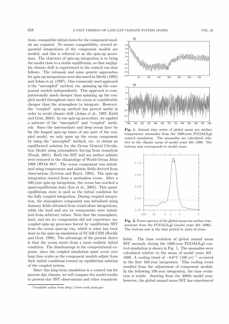
Fig. 1. Annual time series of global mean sea surfacetemperature anomalies from the 1000-year FGOALS glcontrol simulation. The anomalies are calculated rela-tive to the climate mean of model years 401–1000. Thebottom axis corresponds to model years.

Fig. 2. Power spectra of the global mean sea surface tem-perature from the FGOALS gl (model years 401–1000).The bottom axis is the time period in units of years.

fields. The time evolution of global annual meanSST anomaly during the 1000-year FGOALS gl con-trol simulation is shown in Fig. 1. The anomalies werecalculated relative to the mean of model years 401–1000. A cooling trend of −0.6◦C (100 yr)−1 occurredin the first 100-year integration. This cooling trendresulted from the adjustment of component models.In the following 100-year integration, the time evolu-tion is stable. Starting from the 200th model year,however, the global annual mean SST has experienced

aAvailable online from http://www.nodc.noaa.gov


Fig. 3. Mean sea level pressure in (a) northern summer JJA and (b) northern winter DJF averaged overthe last 50 years of the coupled run. For comparison, climatological distribution based NCEP/NCARreanalysis in 1979–1998 is shown in (c) JJA and (d) DJF.

a warming trend of 1.0◦C (100 yr)−1, which was causedby a move from the Lenovo DeepComp 6800 cluster toan IBM SP690 supercomputer, since a “branch” runrather than a ”continue” run setup was employed inthe successive integration on an IBM SP690. Startingfrom the 250th model year, the global mean SST hasexperienced a weak cooling trend which lasted up untilto the 400th model year. In the final 600 years, whichwas performed on the IBM SP690 supercomputer, theevolution of global mean SST is stable, with clear in-terannual variations (Fig. 1b).

The power spectrum of global mean SST anomalyis shown in Fig. 2. A statistically significant peakaround 3–4 year time period is evident. This spec-tral characteristic of model SST is not purely relatedto a strong 3.8-year periodicity in the ENSO variabil-ity as is shown below. Min et al. (2005) show peakpower around the periods of 2 and 3–9 years in ob-served global mean SST. The model has more energyin the 3.8-year period and less power in the periodslonger than 4 years.

4. The atmospheric simulation

The distribution of sea level pressure (SLP) in bo-real winter (December–February, DJF) and summer(June–August, JJA) averaged over the last 50 yearsof the millennial control integration is shown in Fig.3 together with the reanalysis field. The model cap-

tures the overall pattern of reanalysis SLP quite well,except for high-latitude regions in both hemispheres.The JJA subtropical highs in the North Pacific andNorth Atlantic are well simulated for both the posi-tion and strength. Subtropical highs on the SouthernHemisphere during JJA are well positioned, but theyare slightly weaker than the reanalysis. A large neg-ative bias appears in the high-latitudes of the South-ern Hemisphere, suggesting the model is not reliablehere, although the strong biases south of 60◦S mayalso be artifacts caused by large errors in the reanaly-sis SLP in this region (Marshall, 2002). During DJF,the Siberian High in the model is stronger especiallyin the western and northern parts of the high. TheAleutian Low is well reproduced, except that the cen-ter is located more westward. The Icelandic Low isweakly reproduced, with the center of the low locatedmore southward. The SLP is slightly underestimatedover the Southern Ocean.

The annual mean precipitation compared with theGPCP climatology is shown in Fig. 4. The model cap-tures the main features of observed annual mean pre-cipitation, as shown by precipitation maxima in theITCZ, South Pacific and storm track regions of theNorth Atlantic and Pacific and Southern Ocean. Themodel also captures the dry subtropical regions well.Relative to the GPCP climatology, the largest modelerror occurs in the shape of ITCZ. The South PacificConvergence Zone (SPCZ) stretches eastward zonally


Fig. 4. (a) Annual mean precipitation averaged over thelast 50 yrs of the coupled run, and (b) the climate meancondition based on GPCP in 1979–1999.

and appears as a secondary ITCZ in the model. Hencea “double ITCZ” structure dominates the precipita-tion climatology over the tropical oceans. This hasbeen a phenomenon for most coupled models that donot employ flux correction (Yu and Mechoso, 1999;Dai, 2006). Similar bias is also found in the stan-dard version of FGOALS g (Dai, 2006). The ”DoubleITCZ” phenomenon is related to the westward exten-sion of the eastern Pacific cold tongue. Associatedwith the ill-simulated “Double ITCZ” structure, morerainfall develops on both sides of the central Pacificstraddling the equator. Over the western tropical In-dian Ocean, the model produces too much precipita-tion, with errors up to 3 mm d−1. Over the easterntropical Indian Ocean, however, the model producesless precipitation, with errors up to −4 mm d−1. Theprecipitation bias over the South and East Asian mon-soon area appears as a dipole structure: excessive rain-fall is seen along 30◦N over East Asia, while deficientprecipitation develops over South Asia. An artificialrainfall center located to the eastern periphery of theTibetan Plateau is evident in the simulation. A simi-lar bias was found in the standard version of GAMIL,NCAR CCM3 model and NCAR CAM2 model (Yu etal., 2000; Zhang, 2006; Li et al., 2007a). Since theseAGCMs employ an identical convection parameteriza-tion scheme (Zhang and McFarlane, 1995), this com-

mon bias might be related to the treatment of moistconvection in the model, although the steep topogra-phy and the deep continental stratus clouds generatedby the Tibetan Plateau should also have contributions(Yu et al., 2000; Yu et al., 2004). The improved versionof GAMIL shows better results (Li et al., 2007a).

The Asian-Australian Monsoon (A-AM) is one ofthe most dominant monsoon systems in the world(Webster et al., 1998). Following Trenberth et al.(2000, 2006)), we show meridional structures of theoverturning A-AM monsoonal circulations. The A-AM domain is restricted to 60◦–180◦E, covering thewhole Asian-Australian monsoon system. The an-nual cycle of vertical pressure velocity ω at 500 hPais shown in Fig. 5 together with the reanalysis field.The January and July cross sections of the divergentmeridional-circulation component are shown in Fig. 6.

In the reanalysis (Fig. 5b), the ω annual cycleshows more intense phases of the monsoons in Januaryand July–August, with an additional upward motionbranch near 30◦N from April through August that re-flects the elevated Tibetan Plateau heat source and

Fig. 5. The annual cycle of vertical pressure velocity ωat 500 hPa from 50◦S to 50◦N in 10−2 Pa s−1 from (a)FGOALS gl and (b) NCEP/NCAR. Blue indicates up-ward motion and red for subsidence. The bottom axiscorresponds to January to December.


Fig. 6. Regional (60◦–180◦E) meridional cross sections of the divergent flow as vectors from 50◦Sto 50◦N from (a, c) FGOALS gl and (b, d) NCEP/NCAR for January (top) and July (bottom).The scale vector is given at the bottom.

the summer monsoon rainfall in China (e.g., Tao andChen, 1987; Zhou and Li, 2002). This general fea-ture is consistent with that revealed by ERA40 re-analysis (Trenberth et al., 2006). The correspondingcross section (Fig. 6) shows the dominant deep tro-pospheric overturning of the meridional circulation.While the January condition corresponds roughly tothe normal image of the Hadley Cell, for the July con-dition, strong upward motion is evident at 0◦–30◦N.The strong Hadley Cell is replaced by a meridionalcirculation of opposite sense, which is often referred toas the monsoonal meridional cell (Ye and Yang, 1979)and has been used as an observational metric for val-idating AGCMs (e.g., Zhou and Li, 2002). The deepmonsoon cell penetrates upward to 200 hPa.

In the model simulation (Fig. 5a), the ω annualcycle also shows more intense phases of the monsoonsin January and July–August. However, the addi-tional upward motion branch near 30◦N reflecting theEast Asian summer monsoon rainfall persists through-out the year, although it is more intense from Aprilthrough August as in the reanalysis. This upwardmotion bias is consistent with the bias in the rainfallfield. The corresponding cross section (Fig. 6a) showsa weaker subsidence north of 30◦N in January. Themonsoon meridional cell in the simulation penetratesupward to 200 hPa as in the reanalysis, however, it isweaker than the reanalysis, especially for the upwardmotion around 20◦N (cf., Fig. 6c and Fig. 6d).

The seasonal march of the East Asian summermonsoon displays a stepwise northward and northeast-ward advance (Tao and Chen, 1987). The seasonalmigration of the monsoon rain band is represented bythe rainfall zonally averaged between 100◦–120◦E. In

Fig. 7. Seasonal migration of the monsoon rain bandzonally averaged between 100◦–120◦E in (a) observation(GPCP data), and (b) simulation (in units of mm d−1).The bottom axis corresponds to January to December.

observations (Fig. 7a), prior to mid May, south-ern China experiences a pre-monsoon rainy season.The monsoon rain extends from southern Asia to theYangtze River valley in June, and finally penetrates tonorthern China (34◦–41◦N) in July. The rainy season


Fig. 8. (a) Simulated sea surface temperatures averagedover years 951–1000. (b) Difference between the simu-lated SST and HadISST climatological temperatures.

in northern China lasts for about one month and endsin August. From August to September, the monsoonrain belt rapidly moves back to South China (Fig. 7a).The seasonal migration of the monsoon rain band ispoorly reproduced in the simulation (Fig. 7b), mainlybecause an artificial rainfall center is located along30◦N and persists throughout the year. Consequently,the pre-monsoon rainy season over South China in thesimulation is not as strong as that in the observation.For the northward penetration of the monsoon rain-fall band in July, the model result is stronger than theobservation, as indicated by the isoline of 4 mm d−1.The deficiencies in the precipitation simulation are alsoreflected in the soil moisture contents in the contextof both horizontal distribution and seasonal migration(figures not shown). The standard version of GAMILis far better in simulating above observational features(Wang and Ji, 2006; Li et al., 2007a).

5. The oceanic simulation

The decadal average SST from years 951 to 1000 ofthe control run and the difference between the model

Fig. 9. Simulated sea ice concentration averaged overyears 951–1000 in the (a) northern and (b) southern po-lar regions. The thick solid line is the 10% concentrationlimit. (Units: %)

and the HadISST are shown in Fig. 8. The equatorialeastern Pacific cold tongue extends too far westwardin the simulation. A typical artificial structure con-sistent with rainfall, the “double ITCZ” stands out inthe annual mean climatology of SST (Fig. 8a). Overmost of the tropical oceans, the SST biases are lessthan 2 K. Associated with a westward extension ofthe eastern Pacific cold tongue; the central equato-rial Pacific is too cold by 1–2 K. The western Pacificwarm pool region has a weak cold bias of less than1 K. The marine stratus regions off the west coastsof North and South America and off West Africa aretoo warm by 1–3 K. Similar features are reported inthe NCAR CSM (Boville and Gent, 1998) and manyother coupled models (Dai, 2006). The warm SST bi-ases are related to problems in representing the marine


stratus clouds and oceanic upwelling at these regions.In the North Atlantic, a shift in the Gulf Stream isapparent with a warm bias off Labrador, while theSSTs are too cold near Norway. The subtropical west-ern Atlantic is too cold by 2–3 K. Large cold biasesalso develop in the subtropical and high latitudes ofthe North Pacific. These biases are accompanied byshifts in the sea-ice distribution, as shown below. Thehigh-latitude Southern Ocean is too warm by 2–3 K,with the largest bias occuring in the southern IndianOcean (Fig. 8). This is also the region where the SSTobservations are sparse (Rayner et al., 2003).

The distribution of annual-mean sea-ice concentra-tions averaged for model years 951–1000 is shown inFig. 9. The line of the 10% concentration limit inobservations has been given in Kiehl and Gent (2004)(see Fig. 8 of their paper). The sea-ice coverage inthe Northern Hemisphere is acceptable, with too muchsea-ice mainly in the Labrador Sea and Bering Sea.Over the Arctic Ocean, the sea-ice coverage is gener-ally too high. In the Southern Hemisphere, the extentof sea-ice coverage is too large. This excessive sea-icecoverage occurs in both the Atlantic and Pacific sec-tors of the Southern Ocean. Figure 8 shows that theSSTs are too cold in the sub-polar areas of the South-ern Ocean, which allows excessive sea-ice to grow inthe winter. Figure 9 suggests that, while the extentof sea ice is acceptable in FGOALS gl, the biases insea ice concentration are large. It is possible that thebiased sea ice concentration is due to biased sea ice dy-namics, to be specific, sea ice advection velocity beingtoo small.

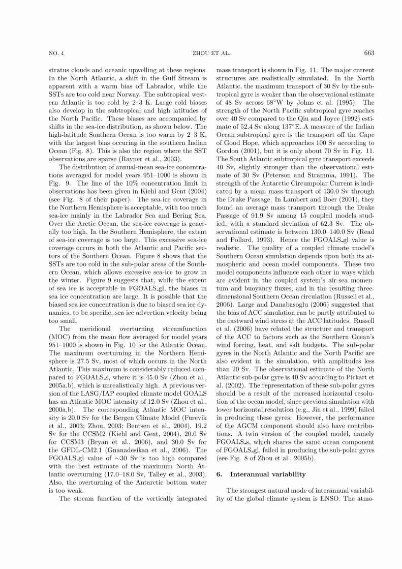
The meridional overturning streamfunction(MOC) from the mean flow averaged for model years951–1000 is shown in Fig. 10 for the Atlantic Ocean.The maximum overturning in the Northern Hemi-sphere is 27.5 Sv, most of which occurs in the NorthAtlantic. This maximum is considerably reduced com-pared to FGOALS s, where it is 45.0 Sv (Zhou et al.,2005a,b), which is unrealistically high. A previous ver-sion of the LASG/IAP coupled climate model GOALShas an Atlantic MOC intensity of 12.0 Sv (Zhou et al.,2000a,b). The corresponding Atlantic MOC inten-sity is 20.0 Sv for the Bergen Climate Model (Fureviket al., 2003; Zhou, 2003; Bentsen et al., 2004), 19.2Sv for the CCSM2 (Kiehl and Gent, 2004), 20.0 Svfor CCSM3 (Bryan et al., 2006), and 30.0 Sv forthe GFDL-CM2.1 (Gnanadesikan et al., 2006). TheFGOALS gl value of ∼30 Sv is too high comparedwith the best estimate of the maximum North At-lantic overturning (17.0–18.0 Sv, Talley et al., 2003).Also, the overturning of the Antarctic bottom wateris too weak.

The stream function of the vertically integrated

mass transport is shown in Fig. 11. The major currentstructures are realistically simulated. In the NorthAtlantic, the maximum transport of 30 Sv by the sub-tropical gyre is weaker than the observational estimateof 48 Sv across 68◦W by Johns et al. (1995). Thestrength of the North Pacific subtropical gyre reachesover 40 Sv compared to the Qiu and Joyce (1992) esti-mate of 52.4 Sv along 137◦E. A measure of the IndianOcean subtropical gyre is the transport off the Capeof Good Hope, which approaches 100 Sv according toGordon (2001), but it is only about 70 Sv in Fig. 11.The South Atlantic subtropical gyre transport exceeds40 Sv, slightly stronger than the observational esti-mate of 30 Sv (Peterson and Stramma, 1991). Thestrength of the Antarctic Circumpolar Current is indi-cated by a mean mass transport of 130.0 Sv throughthe Drake Passage. In Lambert and Boer (2001), theyfound an average mass transport through the DrakePassage of 91.9 Sv among 15 coupled models stud-ied, with a standard deviation of 62.3 Sv. The ob-servational estimate is between 130.0–140.0 Sv (Readand Pollard, 1993). Hence the FGOALS gl value isrealistic. The quality of a coupled climate model’sSouthern Ocean simulation depends upon both its at-mospheric and ocean model components. These twomodel components influence each other in ways whichare evident in the coupled system’s air-sea momen-tum and buoyancy fluxes, and in the resulting three-dimensional Southern Ocean circulation (Russell et al.,2006). Large and Danabasoglu (2006) suggested thatthe bias of ACC simulation can be partly attributed tothe eastward wind stress at the ACC latitudes. Russellet al. (2006) have related the structure and transportof the ACC to factors such as the Southern Ocean’swind forcing, heat, and salt budgets. The sub-polargyres in the North Atlantic and the North Pacific arealso evident in the simulation, with amplitudes lessthan 20 Sv. The observational estimate of the NorthAtlantic sub-polar gyre is 40 Sv according to Pickart etal. (2002). The representation of these sub-polar gyresshould be a result of the increased horizontal resolu-tion of the ocean model, since previous simulation withlower horizontal resolution (e.g., Jin et al., 1999) failedin producing these gyres. However, the performanceof the AGCM component should also have contribu-tions. A twin version of the coupled model, namelyFGOALS s, which shares the same ocean componentof FGOALS gl, failed in producing the sub-polar gyres(see Fig. 8 of Zhou et al., 2005b).

6. Interannual variability

The strongest natural mode of interannual variabil-ity of the global climate system is ENSO. The atmo-


Fig. 10. The annual-mean Atlantic meridional overturning streamfunc-tion (Sv) due to the mean flow averaged over the model year 951–1000.Contour interval is 5 Sv.

Fig. 11. The mean barotropic streamfunction (Sv) due to the meanflow averaged over the years 951–1000.

spheric part of ENSO, the Southern Oscillation, ap-pears as the leading mode of variability when an EOFanalysis is performed on the SLP. Figure 12 shows theleading EOF pattern of SLP in the model simulationand the NCEP/NCAR reanalysis. The EOF mode isshown as a correlation pattern between SLP and theprincipal component. The principal components werecalculated using the area-weighted monthly mean SLPanomalies within 30◦S–30◦N. The leading mode ac-counts for 16.6% of the total variance in the reanalysis.It shows a dipole pattern across the tropical Pacific,where positive SLP anomalies over the western Pacificand Indian Ocean are associated with negative SLP

anomalies spanning a large range of latitudes in theeastern Pacific and extending into the North Atlantic.The EOF1 pattern of FGOALS gl shows a similar ge-ographical distribution (Fig. 12a). It accounts for27.3% of the total variance, which is larger than that ofthe reanalysis. The main deficiency of the simulationis that the signal over the eastern Pacific is too weak.The negative anomalies extending into the North At-lantic are absent in the simulation. The negative SLPanomalies along the Antarctic continent in the simula-tion are stronger than that in the reanalysis. Impactsof ENSO on the Antarctic Oscillation have been foundin the reanalysis (Zhou and Yu, 2004). This impact is


Fig. 12. Upper panels: The distribution of correlation coefficient between the monthly mean globalSLP field and the principal component of EOF1 of monthly mean SLP calculated over the area be-tween 30◦S and 30◦N for (a) FGOALS gl for model years 951–1000 and (b) NCEP/NCAR reanalysis.Lower panels: The time series of the principal components for (c) FGOALS gl and NCEP/NCAR,and (d) the power spectra for the PCs.

Fig. 13. Similar as Fig. 12 except for the SST.

clearly too strong in FGOALS gl. In addition, the ob-served positive anomaly in the southeastern Pacificis weakly simulated by the FGOALS gl. Power spec-tra of the principal components (Fig. 12d) show thatfor periods shorter than 3 years, the FGOALS gl re-sult has more power, while in the period band of 3–10years; there is less power in FGOALS gl compared tothe reanalysis. The maximum power in the reanal-ysis is around 3.5 years and the secondary power is

around 2.8 years. In FGOALS gl, the maximum poweris found at a slightly shorter period of 2.7 years, withthe secondary peak around 3.5 years.

The correlation pattern between SST and the prin-cipal component of SST EOF1 is shown in Fig. 13.A typical El Nino pattern stands out in the observa-tion; the warm anomalies in the eastern tropical Pacificare seen to occur in conjunction with prominent warmanomalies in North Pacific SSTs off the west coast of


Fig. 14. (a) The power spectra and (b) wavelet power spectrum of thesimulated monthly Nino-3.4 index time series during model years 400–1000. The x-axis for panel (a) is the time period in unit of years. They-axis of panel (b) is the Fourier period (in years). The bottom axis isthe time (model year).

North America, as well as with cold anomalies in cen-tral North Pacific. When positive SST anomalies formin the equatorial eastern Pacific, SST anomalies of thesame polarity tend to develop in the tropical IndianOcean, while SST anomalies of reverse polarity de-velop in the western Pacific straddling the equator andextending to the subtropics. Warm anomalies also de-velop in the tropical Atlantic and southeastern Pacific.The simulated pattern closely resembles that of thestandard version of FGOALS g (Wang et al., 2005b;Yu et al., 2005). Compared with the observation, thetongue of warm water along the equator associatedwith El Nino events in the model is too narrow in themeridional direction and stretches too far westward,even arriving in the western Pacific warm pool. Thisis a common problem in many ocean-atmosphere cou-pled models (e.g., Collins et al., 2001; Zhou et al., 2002;Furevik et al., 2003). Another discrepancy of the simu-lation is the warm anomalies to the north of the warmtongue in the western Pacific. Apart from the abovediscrepancies, the simulation shows reasonable agree-

ment with the observation, e.g. positive anomalies areevident in the western tropical Indian Ocean and trop-ical Atlantic (Fig. 13a). The principal component ofthe observation has double spectral peaks on 2.8 and3.5 years, respectively. The 3.5-year peak seems moresignificant than the 2.8-year peak. The first principalcomponent (PC1) simulation exhibits a single spectralpeak around the center of 2.7 years. The El Nino fre-quency in FGOALS gl is slightly higher than that inthe observation. In addition, one typical feature of ElNino in the observation is its irregular frequency. Theoscillation of warm events in the model is too regu-lar (Fig. 13c), and a similar condition is found in thestandard version of FGOALS g (Guilyardi, 2006).

To reveal the possible low-frequency variability,a power spectrum analysis is performed upon themonthly Nino-3.4 index time series covering modelyears 400–1000 (Fig. 14a). It is not surprising to seethat most power concentrates within in the band of 3–4 years. However, one prominent feature, different tothat shown in Fig. 13d, is the multiple-peaks. Periods


Fig. 15. The spatial pattern of EOF1 of NDJFMA(November–April) mean SLP calculated over the re-gion poleward of 20◦N for (a) FGOALS gl and (b)NCEP/NCAR reanalysis. The shading is the regressionof anomalous surface air temperature upon the principalcomponent of EOF1.

either longer than 5 years or shorter than 3 years arealso evident in the long term integration, suggestingboth an irregular frequency and a period transition ofENSO in the coupled model simulation. This featureis further confirmed by employing the Morlet waveletanalysis, as shown in Fig. 14b. A prolonged time pe-riod occurs during model years 680–780. A relativelylonger time scale is also evident during model years800–900. Of importance is the irregular frequency dur-ing the 600-year integration, although previous analy-sis on the final 50-year simulation indicates a regularoscillation (cf. Fig. 13d). This difference suggests therole of internal variability in modulating the ENSOfrequency, since there was no change in the externalforcing agents during the 1000-year integration.

Another strong natural mode of interannual vari-ability of the global climate is the North At-lantic/Arctic Oscillation (NAO/AO), which have been

Fig. 16. The spatial pattern of EOF1 of NDJFMA(November–April) mean SLP calculated over the re-gion poleward of 20◦S for (a) FGOALS gl and (b)NCEP/NCAR reanalysis. The shading is the regressionof anomalous surface air temperature upon the principalcomponent of EOF1.

used as observational metrics for validating climatemodels (e.g. Zhou et al., 2002; Furevik et al.,2003). Recent research revealed the impacts ofNAO/AO on East Asian climate (Gong et al., 2001;Yu and Zhou, 2004; Li et al., 2005; Xin et al.,2006). Figure 15 shows the EOF1 pattern of ND-JFMA (November–April) mean SLP anomalies inFGOALS gl and NCEP/NCAR reanalysis. The lead-ing mode is the well-known Arctic Oscillation dipolepattern. In the reanalysis, anomalous high pressure inthe subtropics is associated with anomalous low pres-sure over the Arctic Ocean and the Nordic Seas (Fig.15b). Following the typical positive AO phase, warmsurface air temperature anomalies over high latitudesof the Eurasian continent are associated with lowerthan normal temperatures centered in the LabradorSea. The southeastern part of North America is dom-


inated by warm anomalies, while northwestern Africais controlled by cold anomalies. The main deficiencyof FGOALS gl in representing AO mode is an artifi-cial high pressure center over the North Pacific. Theanomalous low pressure over the Nordic Seas extendstoo far southward. As a consequence, warm surfaceair temperature anomalies are located in the westernpart of the Eurasian continent, and an artificial coldcenter is found north of the Bering Sea.

The Southern Hemisphere counterpart of the AOis the Antarctic Oscillation (AAO) or Southern Annu-lar Mode (Gong and Wang, 1999). Figure 16 showsthe EOF1 pattern of NDJFMA mean SLP anoma-lies over the Southern Hemisphere in FGOALS gl andNCEP/NCAR reanalysis. The leading mode is theAAO dipole pattern. Anomalous high pressure in thesubtropics is associated with anomalous low pressureover the Antarctic in the reanalysis (Fig. 16b). Warmsurface air temperature anomaly over the subtropicsis associated with lower than normal temperature cen-tered in the Antarctic. The FGOALS gl shows similarpatterns in the AAO mode and the associated surfaceair temperature anomalies as the reanalysis.

7. Summary and concluding remarks

In this paper we have described the mean climate,interannual variability, and long-term trend of a 1000-year control integration of the low resolution versionof the LASG/IAP coupled climate system model us-ing present-constant values of well-mixed greenhousegasses and no external forcing. The fast coupledmodel employs a low-resolution atmospheric compo-nent, GAMIL. The other parts of the model consistof ocean component named LICOM, the land com-ponent, CLM, and the sea ice component from NCARCCSM2. The low-resolution version of the LASG/IAPclimate system model has been run in a fully coupledmode for 1000 years. After the adjustment with acooling trend during the first 150 years, the model hasattained a stable state. However, a change in comput-ers led to further adjustments. During the final 600years of integration, the global mean SSTs have virtu-ally no trend, although the potential shifts of regionalsurface temperature and deep oceans warrant furthervalidation. This is a major achievement for long-termcoupled integrations. The final 600 years of integra-tion are recommended for internal climate variabilitystudies. The strengths and weaknesses of the controlsimulation are summarized as below.

(1) The model captures the main features in theobserved climate. However, the model performancesover the domain poleward of 60◦ in both hemispheresare generally poor, which is ascribed to the low AGCM

resolutions at high-latitudes. The main bias in precip-itation is the “double ITCZ” problem, which led torainfall bias over the maritime continent, tropical In-dian Ocean and the Asian monsoon domain. The biasof model precipitation over the South and East Asianmonsoon area appears as a dipole structure, with ex-cessive rainfall along 30◦N of East Asia and deficientrainfall over South Asia. The artificial rainfall cen-ter located on the eastern periphery of the TibetanPlateau persists throughout the year, which distortsboth horizontal distribution and seasonal migration ofmajor monsoon rain bands over East Asia.

(2) The South Pacific Convergence Zone stretchestoo far eastward in the model, appearing as an artifi-cial “double ITCZ” shape in the climatology of SST.The “double ITCZ” is associated with a westward ex-tension of the eastern Pacific cold tongue. While thecentral equatorial Pacific is too cold by 1–2 K, themarine stratus regions off the western coasts of Northand South America and off of Africa are too warm by1–3 K. Cold biases are evident in the subtropical andhigh latitudes of the North Pacific and the North At-lantic. The Gulf Stream has a warm bias off Labrador.While the extent of sea ice is acceptable, the bias insea ice concentration is large. Apart from the biasesin SST and sea ice simulations, the model is realis-tic in simulating the oceanic 3-dimensional circulation.The maximum meridional overturning streamfunctionin the Atlantic Ocean is 27.5 Sv, which is strongerthan the observational estimate of 17.0–18.0 Sv. Themass transport through the Drake Passage is realistic,with an intensity of 130 Sv. The model also showsreasonable performances in simulating the sub-polargyres over the North Pacific and the North Atlanticexcept with a weaker amplitude compared to the ob-servational estimates.

(3) For the large scale internal interannual vari-ability, focus has been put on the ENSO and annularmodes in both hemispheres. The model shows reason-able performance in simulating the atmospheric part ofENSO, the Southern Oscillation, although the signalover the eastern Pacific is weaker than the reanalysis.The Southern Oscillation accounts for larger variancein the model than in the reanalysis. As the standardversion of the model, a typical El Nino pattern standsout in the simulation; warm anomalies in the east-ern tropical Pacific develop in conjunction with warmanomalies in the North Pacific SSTs, off the west coastof North America, as well as with cold anomalies inthe central North Pacific. Positive SST anomalies de-velop in the western tropical Indian Ocean. However,the tongue of warm water along the equator associ-ated with El Nino events is too narrow in the merid-ional direction and stretches too far westward. The


simulated El Nino has a period of 2.7 years, whichis slightly higher than the observation. The oscilla-tion of warm events in the model is too regular duringmodel years 951–1000, as in the standard version ofthe model. However, an irregular frequency is foundduring the 600-year integration, suggesting the modu-lation of internal variability on the ENSO frequency.

(4) The model captures major features of annu-lar modes, with a better performance for the southernannular mode. The simulated AO mode has an artifi-cial high pressure center over the North Pacific, whichleads to a bias in the associated temperature anoma-lies.

The results presented in this study show that themain aspects of the low resolution coupled solutionare acceptable, although several features of the cou-pled climate are notably far from satisfaction com-pared to the observation or re-analysis and standardversion of the model. Whether or not the shortcom-ings of FGOALS gl climate are acceptable in light ofthe large gains in computational efficiency is a questionthat can only be answered by the individual modeler.This evaluation depends upon the nature of the phe-nomena under investigation. In addition, this papermainly evaluates the model performances in terms ofclimatology and interannual variability, but with pre-liminary analysis on long-term trends and period shiftof El Nino during long-term integration. Some aspectsof the low-frequency variability such as decadal to cen-tennial variations in the Atlantic meridional overturn-ing circulation and Asian Summer Monsoon need tobe quantified in a separate study.

Acknowledgements. This work was jointly sup-

ported by the Chinese Academy of Sciences through

the International Partnership Creative Group entitled

“The Climate System Model Development and Applica-

tion Studies”, the Major State Basic Research Develop-

ment Program of China (973 Program) under Grant No.

2005CB321703, and the National Natural Science Founda-

tion of China (Grant Nos. 40675050, 40221503, 40625014).

The long-term integration of the coupled model was fin-

ished on the Lenovo DeepComp 6800 supercomputer at

the Supercomputing Center of the Chinese Academy of Sci-

ences, and the IBM SP690 at the Institute of Atmospheric

Physics, Chinese Academy of Sciences. The authors ap-

preciate the contribution of Drs. R. C. Yu, Y. Q. Yu, H.

L. Liu, W. P. Zheng, J. Li, X. G Xin, and Mrs. H. Wan,

H. M. Li in the model development and validations.

REFERENCES

Adler, R. F., and Coauthors, 2003: The Version 2 GlobalPrecipitation Climatology Project (GPCP) monthlyPrecipitation analysis (1979–Present). J. Hydrome-

teorology, 4, 1147–1167.Bentsen, M., H. Drange, T. Furevik, and T. Zhou,

2004: Simulated variability of the Atlantic Merid-ional Overturning circulation. Climate Dyn., 22,701–720.

Blackmon, M. B., and Coauthors, 2001: The CommunityClimate System Model. Bull. Amer. Meteor. Soc.,82(11), 2357–2376.

Bonan, G. B., K. W. Oleson, M. Vertenstein, S. Levis,X. Zeng, Y. Dai, R. E. Dickinson, and Z.-L. Yang,2002: The land surface climatology of the Commu-nity Land Model coupled to the NCAR CommunityClimate Model. J. Climate, 15, 3123–3149.

Boville, B. A., and P. R. Gent, 1998: The NCAR Cli-mate System Model, Version One. J. Climate, 11,1115–1130.

Briegleb, B. P., C. M. Bitz, E. C. Hunke, W. H. Lipscomb,M. M. Holland, J. L. Schramm, and R. E. Moritz,2004: Scientific description of the sea ice compo-nent in the Community Climate System Model: Ver-sion Three. NCAR Tech. Note NCARTN-463+STR,70pp.

Bryan, F. O., G. Danabasoglu, N. Nakashiki, Y. Yoshida,D-H. Kim, J. Tsutsui, and S. C. Doney, 2006:Response of North Atlantic thermohaline circula-tion and ventilation to increasing carbon dioxide inCCSM3. J. Climate, 19(11), 2382–2397.

Collins, M., S. F. B. Tett, and C. Cooper, 2001: The in-ternal climate variability of. HadCM3, a version ofthe Hadley Centre coupled model without flux ad-justments. Climate Dyn., 17, 61–81.

Collins, W. D., and Coauthors, 2003: Description of theNCAR Community Atmosphere Model (CAM2). Na-tional Center for Atmospheric Research, Boulder,Colorado, 171pp.

Dai, A., 2006: Precipitation characteristics in eighteencoupled climate models. J. Climate, 19, 4605–4630.

Dai, A., A. Hu, G. A. Meehl, W. M. Washington, and W.G. Strand, 2005: Atlantic thermohaline circulationin a coupled model: Unforced variations vs. forcedchanges. J. Climate, 18, 3270–3293.

Delworth, T. L., R. J. Stouffer, K. W. Dixon, M. J. Spel-man, T. R. Knutson, A. J. Broccoli, P. J. Kushner,and R. T. Wetherald, 2002: Review of simulations ofclimate variability and change with the GFDL R30coupled climate model. Climate Dyn., 19, 555–574.

Furevik, T., M. Bentsen, H. Drange, I. K. T. Kindem,N. G. Kvamsto, and A. Sorteberg, 2003: Descrip-tion and evaluation of the Bergen climate model:ARPEGE coupled with MICOM. Climate Dyn., 21,27–51.

Frank, R., 2001: An atlas of surface flues based onthe ECMWF reanalysis: A climatological datasetto force global ocean general circulation models. Re-port No. 323, Max-Planck-Institute for Meteorology,Hamburg, 31pp.

Gnanadesikan, A., and Coauthors, 2006: GFDL’s CM2Global Coupled Climate Models. Part II: The base-line ocean simulation. J. Climate, 19, 675–697.


Gent, P. R., and J. C. McWilliams, 1990: Isopycnal mix-ing in ocean circulation models. J. Phys. Oceanogr.,20, 150–155.

Gong, D. Y., and W. S. Wang, 1999: Definition of Antarc-tic Oscillation index. Geophys. Res. Lett., 26, 459–462.

Gong, D. Y., S. H. Wang, and J. H. Zhu, 2001: EastAsian winter monsoon and Arctic Oscillation. Geo-phys. Res. Lett., 28, 2073–2076.

Gordon, A., 2001: Interocean exchange. Ocean Circula-tion and Climate. Vol. 77, International GeophysicsSeries, Academic Press, 303–314.

Guilyardi, E., 2006: El Nino-mean state-seasonal cycle in-teractions in a multi-model ensemble. Climate Dyn.,26, 329–348.

IPCC, 2007: Climate Change 2007: The Physical Sci-ence Basis. Contribution of Working Group I to theFourth Assessment Report of the IntergovernmentalPanel on Climate Change, Solomon et al., Eds., Cam-bridge University Press, Cambridge, United King-dom and New York, USA, 996pp.

Jacob, R., C. Schafer, I. Foster, M. Tobis, and J. An-derson, 2001: Computational design and perfor-mance of the Fast Ocean Atmosphere Model, Ver-sion One. Proc. International Conference on Com-putational Science, Alexandrov et al., Eds., Springer-Verlag, 175–184.

Jin, X. Z., X. H. Zhang, and T. J. Zhou, 1999: Fundamen-tal framework and experiments of the third genera-tion of IAP/LASG World Ocean General CirculationModel. Adv. Atmos. Sci., 16, 197–215.

Johns, W., T. Shay, J. Bane, and D. Watts, 1995: GulfStream structure, transport, and recirculation near68◦W. J. Geophys. Res., 100, 817–838.

Johns, T. C., R. E. Carnell, J. F. Crossley, J. M. Gregory,J. F. B. Mitchell, C. A. Senior, S. F. B. Tett, and R.A. Wood, 1997: The Second Hadley Centre coupledocean-atmosphere GCM: Model description, spinupand validation. Climate Dyn., 13, 103–134.

Jones, C., J. Gregory, R. Thorpe, P. Cox, J. Murphy, D.Sexton, and P. Vlades, 2005: Systematic optimiza-tion and climate simulations of FAMOUS, a fast ver-sion of HadCM3. Climate Dyn., 25, 189–204.

Kalnay, E., and Coauthors, 1996: The NCEP/NCAR 40-year reanalysis project. Bull. Amer. Meteor. Soc., 77,437–472.

Kiehl, J. T., and P. R. Gent, 2004: The Community Cli-mate System Model, Version Two. J. Climate, 17,3666–3682.

Lambert, S. J., and G. J. Boer, 2001: CMIP1 evaluationand inter-comparison of coupled climate models. Cli-mate Dyn., 17, 83–106.

Large, W. G., and G. Danabasoglu, 2006: Attributionand impacts of upper ocean biases in CCSM3. J. Cli-mate, 19, 2325–2346.

Levitus, S., and T. P. Boyer, 1994: World Ocean Atlas1994: Temperature and Salinity. U. S. Departmentof Commerce, Washington, D.C., 117pp.

Li, J., R. Yu, T. Zhou, and B. Wang, 2005: Why is there

an early spring cooling shift downstream of the Ti-betan Plateau. J. Climate, 18, 4660–4668.

Li, L. J., B. Wang, Y. Q. Wang, and H. Wan, 2007a:Improvements in climate simulation with modifi-cations to the Tiedtke convective parameterizationin the grid-point atmospheric model of IAP LASG(GAMIL). Adv. Atmos. Sci., 24, 323–335, DOI:10.1007/s00376-007-0323-3.

Li, L., B. Wang, and T. Zhou, 2007b: Contribu-tions of natural and anthropogenic forcings tothe summer cooling over eastern China: AnAGCM study. Geophys. Res. Lett., 34, L18807,doi:10.1029/2007GL030541.

Li, L., B. Wang, and T. Zhou, 2007c: Impacts of externalforcing on the 20th century global warming. ChineseScience Bulletin, 52, 3148–3154.

Li, Z. X., and S. Conil, 2003: A 1000-year simulation withthe IPSL ocean-atmosphere coupled model. Annalsof Geophysics, 46, 39–46.

Liu, H., X. Zhang, W. Li, Y. Yu, and R. Yu, 2004: Aneddy-permitting oceanic general circulation modeland its preliminary evaluations. Adv. Atmos. Sci.,21, 675–690.

Manabe, S., and R. J. Stouffer, 1996: Low-frequency vari-ability of surface air temperature in a 1000-year inte-gration of a coupled atmosphere-ocean-land surfacemodel. J. Climate, 9, 376–393.

Marshall, G. J., 2002: Trends in Antarctic geopotentialheight and temperature: A comparison between ra-diosonde and NCEP-NCAR reanalysis data. J. Cli-mate, 15, 659–674.

Meehl, A. M., 1995: Global coupled general circulationmodels. Bull. Amer. Meteor. Soc., 76, 951–957.

Min, S. K., S. Legutke, A. Hense, and W. T. Kwon, 2005:Internal variability in a 1000-yr control simulationwith the coupled climate model ECHO-G—I. Near-surface temperature, precipitation and mean sea levelpressure. Tellus, 57A, 605–621.

Montoya, M., A. Griesel, A. Levermann, J, Mignot, M.Hofmann, A. Ganopolski, and S. Rahmstorf, 2005:The earth system model of intermediate complex-ity CLIMBER-3a. Part I: Descrippdftion and per-formance for present day conditions. Climate Dyn.,25, 237–263.

Pacanowski, R. C., and G., Philander, 1981: Parameter-ization of vertical mixing in numerical models of thetropical ocean. J. Phys. Oceanogr., 11, 1442–1451.

Peterson, R., and L. Stramma, 1991: Upper-level cir-culation in the South Atlantic Ocean. Progress inOceanography, 26, 1–73.

Pickart, R., D. Torres, and R. Clarke, 2002: Hydrogra-phy of the Labrador Sea during active convection. J.Phys. Oceanogr, 32, 428–457.

Qiu, B., and T. Joyce, 1992: Interannual variability inthe mid- and low-latitude western North Pacific. J.Phys. Oceanogr, 22, 1062–1079.

Rayner, N. A., D. E. Parker, E. B. Horton, C. K. Folland,L. V. Alexander, D. P. Rowell, E. C. Kent, and A.Kaplan, 2003: Globally complete analyses of sea sur-


face temperature, sea ice and night marine air tem-perature, 1871–2000. J. Geophys. Res., 108, 4407,doi:10.1029/2002JD002670.

Read, J. F., and R. T. Pollard, 1993: Structure and trans-port of the Antarctic circumpolar current and Ag-ulhas return current at 40E. J. Geophys. Res., 98,12281–12295.

Rosati, A., and K., Miyakoda, 1988: A general circu-lation model for upper ocean circulation. J. Phys.Oceanogr., 18, 1601–1626.

Russell, J. L., R. J. Stouffer, and K. W. Dixon, 2006:Intercomparison of the southern ocean circulation inIPCC coupled model control simulations. J. Climate,19, 4560–4575.

Talley, L. D., J. L. Reid, and P. E. Robbins, 2003: Data-based meridional overturning streamfunctions for theglobal ocean. J. Climate, 16, 3213–3226.

Tao, S., and L. Chen, 1987: A review of recent research onthe East Asian summer monsoon in China. MonsoonMeteorology, C. P. Chang and T. N. Krishnamurti,Eds., Oxford University Press, 60–92.

Trenberth, K. E., D. P. Stepaniak, and J. M. Caron, 2000:The global monsoon as seen through the divergentatmospheric circulation. J. Climate, 13, 3969–3993.

Trenberth, K. E., J. W. Hurrell, and D. P. Stepaniak,2006: The Asian monsoon: Global perspective. TheAsian Monsoon, Springer/Praxis Publishing, NewYork, 67–87.

von Storch, J.-S., V. V. Kharin, U. Cubasch, G. C.Hegerl, D. Schriever, H. von Storch, and E. Zorita,1997: A description of a 1260-year control integrationwith the coupled ECHAM1/LSG general circulationmodel. J. Climate, 10, 1525–1543.

Wang, B., and Coauthors, 2004: Design of a new dy-namical core for global atmospheric models based onsome efficient numerical methods. Scence in China(Ser. A), 47, 4–21.

Wang, B., and Z. Z. Ji, 2006: Studies and Applicationsof New Numerical Methods in Atmospheric Sciences.Science Press, Beijing, 208pp. (in Chinese)

Wang, B., and Coauthors, 2005b: Recent progress in thedevelopment of the 4th generation of LASG/IAP cli-mate system model FGOALS and the associated ex-periments. 2005 Annual Meeting of the Institute ofAtmospheric Physics, Chinese Academy of Sciences,Beijing.

Wang, Y., L. A. Mysak, Z. Wang, and V. Brovkin, 2005a:The greening of the McGill paleoclimate model, PartI: Improved land surface scheme with vegetation dy-namics. Climate Dyn., 24, 469–480.

Wang, Z., and L. A. Mysak, 2000: A simple coupledatmosphere-ocean-sea ice-land surface model for cli-mate and paleoclimate studies. J. Climate, 13, 1150–1172.

Wang, Z., and L. A. Mysak, 2002: Simulation of thelast glacial inception and rapid ice sheet growth inthe McGill Paleoclimate Model. Geophys. Res. Lett.,29(23), doi: 10.1029/ 2002GL015, 120.

Webster, P. J., Magana, V. O., and Palmer, T. N.,

1998: Monsoon: Processes, predictability, and theprospects for prediction. J. Geophys. Res., 103,14451–14510.

Wen, X., T. Zhou, S. Wang, B. Wang, H. Wan, and J.Li, 2007: Performance of a reconfigured atmosphericgeneral circulation model at low resolution. Adv. At-mos. Sci., 24, 712–728, 10.1007/s00376-007-0712-7.

Wu, L., Z. Liu, R. Gallimore, R. Jacob, D. Lee, and Y.Zhong, 2003: Pacific decadal variability: the TropicalPacific mode and the North Pacific mode. J. Climate,16, 1101–1120.

Wu, L., D. Lee, and Z. Liu, 2005: The 1976/77 North Pa-cific climate shift: The role of subtropical ocean ad-justment and coupled ocean-atmosphere feedbacks.J. Climate, 18, 5125–5140.

Wu, G., H. Liu, Y. C. Zhao, and W. P. Li, 1996: A nine-layer atmospheric general circulation model and itsperformance. Adv. Atmos. Sci., 13, 1–18.

Xin, X., R. Yu, T. Zhou, and B. Wang, 2006: Droughtin Late Spring of South China in Recent Decades. J.Climate, 19, 3197–3206.

Ye, D. Z., and G. J. Yang, 1979: Mean meridional cir-culations over East Asia and the Pacific Ocean. I:summer; II: Winter. Chinese Journal of AtmosphericScientific Sciences, 3, 299–305. (in Chinese)

Yeager, S. G., C. A. Shields, W. G. Large, and J. J. Hack,2006: The Low-Resolution CCSM3. J. Climate, 19,2545–2566.

Yu, J. Y., and C. R. Mechoso, 1999: Links between an-nual variations of Peruvian stratocumulus clouds andof SST in eastern equatorial Pacific. J. Climate, 12,3305–3318.

Yu, R., and T. Zhou, 2004: Impacts of winter-NAO onMarch cooling trends over subtropical Eurasia conti-nent in the recent half century. Geophys. Res. Lett.,31, L12204, doi:10.1029/2004GL019814.

Yu, R., W. Li, X. Zhang, Y. Yu, and T. Zhou, 2000:Climatic features related to eastern China summerrainfalls in the NCAR CCM3. Adv. Atmos. Sci., 17,503–518.

Yu, Y., R. Yu, X. Zhang, and H. Liu, 2002: A FlexibleGlobal Coupled Climate Model. Adv. Atmos. Sci.,19, 169–190.

Yu, R., B. Wang, and T. Zhou, 2004: Climate effectsof the deep continental stratus clouds Generated byTibetan Plateau. J. Climate, 17, 2702–2713.

Yu, Y. Q., and Coauthors, 2005: IAP global coupled cli-mate model FGOALS and its application in climatechange. MOST-DOE Science Team Meeting, Beijing.

Zhang, G. J. and N. A. McFarlane, 1995: Sensitivity ofclimate simulations to the parameterization of cumu-lus convection in the Canadian Climate Centre gen-eral circulation model. Atmos.-Ocean, 33, 407–446.

Zhang, W. J., 2006: Spatial distribution and temporalvariation of the observed and simulated soil mois-ture over China. M. S. thesis, Institute of Atmo-spheric Physics, Chinese Academy of Sciences, Bei-jing, 119pp. (in Chinese)

Zhang, X., and J. E. Walsh, 2006: Toward a seasonally


ice-covered Arctic Ocean: Scenarios from the IPCCAR4 model simulations. J. Climate, 19, 1730–1747.

Zhou, T., 2003: Multi-spatial variability modes of the At-lantic Meridional Overturning Circulation. ChineseScience Bulletin, 48(Suppl. II), 30–35.

Zhou, T., and Z. X. Li, 2002: Simulation of the EastAsian summer monsoon by using a variable resolu-tion atmospheric GCM. Climate Dyn., 19, 167–180.

Zhou, T., and R. Yu, 2004: Sea-surface temperature in-duced variability of the Southern Annular Mode inan atmospheric general circulation model. Geophys.Res. Lett., 31, L24206,doi:10.1029/2004GL021473.

Zhou, T. and R. Yu, 2006: Twentieth century surface airtemperature over China and the globe simulated bycoupled climate models. J. Climate, 19(22), 5843–5858.

Zhou, T., X. Zhang�R. Yu, Y. Yu, and S. Wang, 2000c:The North Atlantic oscillation simulated by Version2 and 4 of IAP/LASG GOALS Model. Adv. Atmos.Sci., 17, 601–616.

Zhou, T., X. Zhang, and S. Wang, 2000a: The relation-ship between the thermohaline circulation and cli-mate variability. Chinese Science Bulletin, 45(11),

1052–1056.Zhou, T., X. Zhang, Y. Yu, R. Yu, and S. Wang, 2000b:

Response of IAP/LASG GOALS model to the cou-pling of air-sea freshwater exchange. Adv. Atmos.Sci., 17(3), 473–486.

Zhou, T., R. Yu, and Z. Li, 2002: ENSO-dependentand ENSO-independent variability over the mid-latitude North Pacific: Observation and Air-sea cou-pled model simulation. Adv. Atmos. Sci., 19, 1127–1147.

Zhou, T. J., R. C. Yu, Z. Z. Wang, and T. W. Wu, 2005a:The Atmospheric General Circulation Model SAMILand the Associated Coupled Model FGOALS s, Me-teorology Press, Beijing, 288pp. (in Chinese)

Zhou, T. J., and Coauthors, 2005b: The climate systemmodel FGOALS s using LASG/IAP spectral AGCMSAMIL at its atmospheric component. Acta Meteo-rologica Sinica, 63(5), 702–715. (in Chinese)

Zhou, T., Y. Yu, H. Liu, W. Li, X. You, and G. Zhou,2007: Progress in the development and applicationof climate ocean models and ocean-atmosphere cou-pled models in China. Adv. Atmos. Sci., 24(6), 1109–1120, DOI: 10.1007/s00376-007-1109-3729–738.

a fast version of lasg/iap climate system model and … in atmospheric sciences, vol. 25, no. 4,...

Documents