N A S A C O N T R A C T O R

R E P O R T

COCM

N A S A C R - 2 3 9 1

CO

<C

A FINITE ELEMENT SOLUTION ALGORITHM

FOR THE NAVIER-STOKES EQUATIONS

by A. J. Baker

Prepared by

BELL AEROSPACE COMPANY

Buffalo, N.Y. 14240

for Langley Research Center

NATIONAL AERONAUTICS AND SPACE ADMINISTRATION • WASHINGTON, D. C. • JUNE 1974

https://ntrs.nasa.gov/search.jsp?R=19740020922 2018-05-12T19:11:51+00:00Z

1. Report No. 2. Government Accession No.

NASA CR-23914. Title and Subtitle

A Finite Element Solution Algorithm for theNavier-Stokes Equations

7. Author(s)

A.J. Baker9. Performing Orgoniiotion Nome ond Address

Bell Aerospace CompanyP.O. Box OneBuffalo, New York 14240

12. Sponsoring Agency Nome ond Address

National Aeronautics and Space AdministrationWashington, D.C. 20546

3. Recipient's Catalog No.

5. Report Date

June 19?6. Performing Organization Code

8. Performing Organization Report No.

D9 198-9 5000110. Work Unit No.

11. Contract or Grant No.

NAS 1-11809

Contractor Report

14. Sponsoring Agency Code

15. Supplementory Notes

Final Report

16. AbstractA finite element solution algorithm is established for the two-dimensional Navier-Stokes equa-

tions governing the steady-state kinematics and thermodynamics of a variable viscosity, compressiblemultiple-species fluid. For an incompressible fluid, the motion may be transient as well. The primi-tive dependent variables are replaced by a vorticity-streamfunction description valid in domainsspanned by rectangular, cylindrical and spherical coordinate systems. Use of derived variables pro-vides a uniformly elliptic partial differential equation description for the Navier-Stokes system, and fowhich the finite element algorithm is established. Explicit non-linearity is accepted by the theory,since no psuedo-variational principles are employed, and there'is no requirement for either computa-tional mesh or solution domain closure regularity: Boundary condition constraints on the normal fluxand tangential distribution of all computational variables, as well as velocity, are routinely piecewiseenforceable on domain closure segments arbitrarily oriented with respect to a global reference frame.

A natural coordinate function description is established for the finite element approximationfunctions that renders matrix evaluation straightforward and accurate. The several explicitly non-linear terms in the equation system are shown to be expressible in terms of standard matrix forms.The consequence of integrating various terms by parts is thoroughly evaluated. The COMOC com-puter program system embodies the established finite element algorithm and matrix generator packagibuilt upon the natural function description. Numerical solutions for incompressible internal flowproblems have illustrated solution accuracy, convergence, and versatility. Flow fields with imbeddedregions of recirculation have been computed as well as transient solution domain closure shapes.

•Evaluation of pressure computations has been performed as well as extension to compressible flowfield solutions.

17. Key Words (V lected by Author(s))

Finite ElementNavier-Stokes EquationsNatural Coordinate FunctionsComputer Program

19. Security Ctossif. (of this report)

Unclassified

18. Distribution Statement

Unclassified - Unlimited

20. Security Clossif. (of this page) 21. No. ol

Unclassified 7

Pages 22. Price*

5 $3.75

For sale by the National Technical Information Service, Springfield, Virginia 22151

Page Intentionally Left Blank

CONTENTS

Page

SUMMARY 1INTRODUCTION 1NOMENCLATURE 3THE NAVIER-STOKES EQUATIONS FOR A MULTICOMPONENT VISCOUS FLUID . . 6DIFFERENTIAL EQUATION DEVELOPMENT FOR THE DESIRED PROBLEM

CLASS IN FLUID MECHANICS 8Continuity Equation 8Compatibility Equation 10The Curl of the Navier-Stokes Equation 10The x3 Component of the Navier-Stokes Equation 13The Species Continuity Equation 14The Energy Equation 14Recovery of Pressure 16

FINITE^ELEMENT SOLUTION ALGORITHM FOR THE NAVIER-STOKESEQUATIONS 18

FINITE ELEMENT MATRIX GENERATION , 22Planar Finite Elements for the Two-Dimensional Navier-Stokes Equations 25Planar Ring Finite Elements for the Axisymmetric Incompressible Navier-Stokes

Equations 31COMOC COMPUTER PROGRAM ' 34NUMERICAL RESULTS 34CONCLUDING REMARKS 54APPENDIX A: CARTESIAN TENSORS IN EUCLIDEAN SPACE 59APPENDIX B: OBSERVATIONS ON THE FINITE ELEMENT SOLUTION

ALGORITHM FOR THE NAVIER-STOKES EQUATIONS USINGLINEAR NATURAL COORDINATE APPROXIMATION (

FUNCTIONALS 62APPENDIX C: SYSTEM INVARIANCE UNDER COORDINATE

TRANSFORMATION 69REFERENCES 72

111

ILLUSTRATIONS

Figure Page

1 Intrinsic Finite Element Domains for Simplex Approximation Functions 232 Establishment of Vorticity Boundary Condition Statement 313 Discretization of Rectangular Duct into 144 Triangular Finite Elements 354 Computed Fully Developed Longitudinal Velocity Distributions, Re = 200 ... 365 Computed Fully Developed Streamfunction and Vorticity for Duct Flow,

Re = 200 : • 376 Longitudinal Velocity Distributions for Incompressible Duct Flow, Re = 200. . . 387 Computed Transient Temperature Distribution in Axisymmetric Quiescent

Duct 408 Discretization Influence on Vorticity and Streamfunction Near a Wall 419 Discretization Influence on Computed Streamfunction 4210 Flow Over a Rearward Facing Step 4311 Discretization of Rearward Facing Step in a Rectangular Duct into 211

Triangular Finite Elements 441 2 COMOC Computed Streamfunction and Vorticity Distribution for Transient

Flow Over a Rearward Facing Step 4513 COMOC Computed Steady-State Streamfunction and Vorticity for Flow Over

a Rearward Step in Irregular Shaped Duct, and Over a Rearward Step withInternal obstacle, Re = 200 47

14 Centerplane Pressure Decay in Steady-State Duct Flow, Re = 200 4915 Centerplane Pressure Distribution for Steady Flow Over a Rearward Facing

Step, Re = 200. . . 5016 Flow into a Compression Corner 521 7 Supersonic Flow Over a Rearward Facing Cone-Step 5218 Computed Steady-State Distributions for Compressible Flow Over a

Rearward Step, Re = 200, MOO = 0.6. . ; ; •. 5519 Finite Element Discretizations for Supersonic Boundary Flows •. . . 5620 Computed Steady-State Distributions for Supersonic Boundary Layer

Flow, Moo = 3.0 57B-l Two-Dimensional Finite Element ' . . . . . . . . 63B-2 Adjacent Finite Elements 65C-l Coordinate Systems for the Finite Element Solution Algorithm 70

TABLES

Number . Page

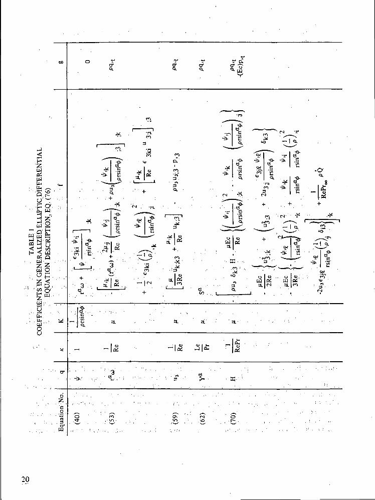
1 Coefficients in Generalized Elliptic Differential Equation Description,Equation (76) 20

2 Implicit Definition of Simplex Natural Coordinate Functions 243 Integrals of Natural Coordinate Function Products Over Finite Element

Domains 244 Standard Finite Element Matrix Forms for Simplex Functional in Two-

Dimensional Space 265 Additional Standard Matrix Forms for Simplex Functional in Axisymmetric

Space : 33

IV

A FINITE ELEMENT SOLUTION ALGORITHMFOR THE NAVIER-STOKES EQUATIONS

ByA.J. Baker

Bell Aerospace Company

SUMMARY

A fini te element solution algorithm is established for the two-dimensional Navier-Stokes equa-tions governing the steady-state kinematics and thermodynamics of a variable viscosity, compressiblemultiple-species fluid. For an incompressible fluid, the motion may be transient as well. The primi-tive dependent variables are replaced by a vorticity-streamfunction description valid in domains span-ned by rectangular, cylindrical and spherical coordinate systems. Use of derived variables provides auniformly elliptic partial differential equation description for the Navier-Stokes system, and forwhich the finite element algorithm is established. Explicit nonlinearity is accepted by the theory,since no psuedo-varjational principles are employed, and there is no requirement for either compu-tational mesh or solution domain closure regularity. Boundary condition constraints on the normalflux and tangential distribution of all computational variables, as well as velocity, are routinelypiecewise enforceable on domain closure segments arbitrarily oriented with respect to a global ref-erence frame.

A natural coordinate function description is established for the finite element approximationfunctions that renders matrix evaluation straightforward and accurate. The several explicitly non-linear terms in the equation system are shown to be expressible in terms of standard matrix forms.The consequence of integrating various terms by parts is thoroughly evaluated. The COMOC com-puter program system embodies the established finite element algorithm and matrix generator pack-age built upon the natural function description. Numerical solutions for incompressible internal flowproblems have illustrated solution accuracy, convergence, and versatility. Flow fields with imbeddedregions of recirculation have been computed as well as transient solution domain closure shapes.Evaluation of pressure computations has been performed as well as extension to compressible flowfield solutions.

INTRODUCTION

Numerical solution of a variety of field problems in mechanics has been made possible withthe advent of the large digital computer. Development of solution procedures for specific disciplineshas been highly problem oriented. As a result, little cross-fertilization has occurred that takes advan-tage of the uniform mathematical description for field problems in continuum mechanics. Specifi-cally, finite difference methods have been almost universally employed for computational fluid mech-anics, the electric analogy approach has been applied to heat conduction and seepage problems, whilethe finite element method has found wide acceptance for analysis of complex structural systems. Eachof these approaches can now be viewed in a unifying manner as application of specific criteria withinthe Method of Weighted Residuals (MWR) (Reference 1), and satisfaction in a weighted average senseof the governing differential equations written on the discretized equivalent of the pertinent depend-ent variables. The select choice of weighting and approximation functions renders each approach identi-

fiable, including classical integral approaches like von Karman-Pohlhausen and Integral Method ofStrips in boundary layer flow, and the many variations of Galerkin, Kantorovich and collocationmethods.

Over the years, the finite element procedure has proven highly adaptable to solution of linearelliptip boundary value problems involving complex boundary conditions applied on irregularlyshaped, non-coordinate surface solution domain closures. Its adaptation to quasilinear and/or nonlin-ear problem classes — for example, solution of the Navier-Stokes equations'— has been held in abey-ance, at least partially, by the, common misconception that the method was constrained to problemshaving a differential equation description that could be equivalently cast into an extremization prin-ciple. This in turn led to derivation of a plethora of psuedo-variational statements for nonstationaryfield problems (see for example Reference 2) in an attempt to render the finite element method direct-ly applicable to the broader problem class. Finite element solution of transient linear heat conductionin stationary continua drew much attention in the late 1960's (References 3, 4), and inclusion ofimplicit nonlinearity was eventually acceptable (Reference 5) within the constraints of "local" ex-tremization. Extension to the Navier-Stokes equations using these concepts appeared theoreticallydifficult without gross assumptions on the concept of a local potential. However, about 1970 theconnection between Galerkin criteria within MWR and equivalent extremization principles wasestablished, the key items being performance of an integration by parts, identification of a numericalLagrange multiplier, and Boolean assembly of the local finite element matrix equations into the glob-al description. It could be readily proved that such a development, for a linear equation, produced acomputational form that was identical to extremization of the equivalent stationary principle. How-ever, since no linearity constraint existed in its derivation, the theory for finite element solution ofnonlinear equations was established, especially for specific forms of the Navier-Stokes equations(References 6-8).

In this report, a finite element solution algorithm is established for the two-dimensionalNavier-Stokes equations governing the kinematics and thermodynamics of a variable viscosity, com-

' pressible, multiple-species fluid. The primitive dependent variables are replaced by a vorticity-streamfunction description, which provides a uniformly elliptic differential equation system descrip-tion for all computational variables. The preferred differential equation systems are established inrectangular, cylindrical and spherical Cartesian coordinate systems. The finite element algorithm isderived for the generalized, nonlinear elliptic boundary value problem of mathematical physics andcontains no requirements for either computational mesh or solution domain closure regularity.Boundary condition constraints on the normal flux and tangential distribution of all computationaldependent variables, as well as velocity, are routinely piecewise enforceable on domain closuresegments arbitrarily oriented with respect to a global reference frame. The intrinsic finite elementshapes for one-, two-, and three-dimensional domains spanned by linear approximation functions arethe line, triangle and tetrahedron respectively. The area-coordinate concept of structural mechanicshas been utilized to establish a natural coordinate function description for the finite element approx-imation to the Navier-Stokes equations. Adaptation of these functions represents a significant advancethat has for the first time allowed analytical formulation of the complexly nonlinear matrix repre-sentations for specific terms in the equation system — in particular, the vorticity transport equation.The consequence of integration by parts of select nonlinear terms in the differential equation systemis examined in detail, and the assumptive constraints are established according to which the generatedsurface integrals can be neglected or made to cancel. Establishment of the natural coordinate func-tion description has allowed recognition of the many standard matrix forms that constitute.the finiteelement algorithm for the nonlinear terms in the equation system and provides broad insight into themechanics of the algorithm.

The finite element solution algorithm for the characteristic equation system has been embod-ied into the COMOC (Computational Continuum Mechanics) computer program system, specific var-iants of which have produced solutions in three-dimensional subsonic and supersonic viscous flow fields(References 9, 10) and nonlinear transient heat conduction (Reference 11) in addition to the Navier-Stokes solutions to be discussed. The COMOC system consists of four basic macro-modules, the firstof which is Input wherein discretizations are formed and dependent variables initiated. The Geometrymodule establishes the non-standard element matrices for each finite element of the discretization andevaluates the matrix multipliers required for the standard matrices. All computations are performedin a local Cartesian coordinate system with automatic accounting for the lack of coordinate trans-formation invariance for other than rectangular Cartesian systems. The Integration module embodiessolution algorithms for large-order ordinary differential and algebraic equation systems, either ofwhich is produced by application of the finite element algorithm to the parent partial differentialequation system. For discretized-equivalent initial value problems, the basic operation is evaluationof the derivative vector on an element basis and assembly of the global vector using Boolean algebra.For solution of an algebraic system, the diffusion (that is, "stiffness" in elasticity) matrix is formedon an element basis and the equation system inhomogeniety evaluated, if present. Each is thenassembled into the global representation through Boolean algebra. The matrix equation system rankis established by evaluating boundary condition constraints, and the effective inverse found by equa-tion solver techniques. The final Output module serves its standard function.

The Navier-Stokes Variant of COMOC has been evaluated for several problems to assess solu-tion accuracy, convergence, versatility, and overall performance of the system. Accuracy studieswere performed for developing flow in a duct, and convergence of velocity with discretization isnumerically demonstrated. Factors affecting solution accuracy have been evaluated including non-uniform discretizations, the vorticity boundary condition, arid the use of a "condensed" mass matrixfor solving transient problems. A basic character of full Navier-Stokes solutions is prediction of im-bedded regions of recirculation, and the finite element algorithm is assessed to correctly predict suchphenomena for a sample problem without resorting to special boundary condition techniques. Astable solution for the rearward step problem has been obtained for the largest flow Reynolds numberreported in the literature. Variations on this problem have illustrated stable solutions for time-depend-ent solution domain closure configurations and solutions in multiply-connected domains. Evaluationof the accuracy of pressure computations for these problems is presented as well as extension to flowfields with variable density. The computed results have yielded a favorable assessment of the viabilityof the solution algorithm and its computational embodiment.

NOMENCLATURE

a boundary condition coefficient; unit vector

b body force unit vector

B body force

c expansion coefficient; specific heat

D diffusion coefficient

e general alternating tensor

E symmetric velocity gradient

EC Eckert Number

f function of known argument

Fr Froude Number

g mass flow; function of known argument

h metric coefficient

H stagnation enthalpy

i j,k rectangular Cartesian unit vectors

J determinant of Cartesian space metric v

k function of known argument; thermal conductivity

K generalized diffusion coefficient

L characteristic length; natural coordinate function; arc length

Le • .Lewis Number

M -Mach Number; number of finite elements

n unit normal vector; summation limit

N differential operator

p pressure

Pr Prandtl Number

Q,q generalized dependent variable; energy source term

-Ir, 0, 0} spherical Cartesian coordinate system

r position vector; radius

R domain of space variables; gas constant

Re Reynolds Number

s displacement :

S mass source term .

t time

T temperature; total stress tensor; tensor

u, U velocity

v vector

W weighting function

jx, y ,z | rectangular Cartesian coordinate system

x independent space variables

y rectangular Cartesian scalar componentsi •

Y mass fraction

jz, r, 61 cylindrical Cartesian coordinate system

a coefficient for spherical coordinates; mass fraction; direction cosine

-y ratio of specific heats

r finite element coefficient matrix

5 Kronecker delta

3R closure of solution domain

e alternating tensor; strain; vector

TJ differential operator

8 angle

K coefficient

X Lagrange multiplier

/z viscosity

v unit normal vector

p : density | i

a surface integral kernel

T stress tensor; domain integral kernel

0 angle; function

i// x3 scalar component of streamfunction

ty vector potential

co x3 scalar component of vorticity; wryness coefficient

vorticity vector

column matrix

square matrix

diagonal matrix

Superscripts and Subscripts

* approximate solution

temporal derivative

T matrix transposeA unit vector

-* vector

— average; constrained to domain closure

i,j ,k, 2 tensor indices

m pertaining to mtn subdomain (finite element)

oo reference condition

THE NAVIER-STOKES EQUATIONS FOR A MULTICOMPONENTVISCOUS FLUID

The complete description of a fluid dynamical state is contained within the solution of thesystem of coupled, nonlinear, second order partial differential equations describing the local con-servation of species, mass, linear (or angular) momentum, and energy, in conjunction with an appro-priate specification of constitutive behavior and applicable initial and boundary conditions. InCartesian tensor notation (see Appendix A) the conservation form of these differential equations isrespectively

a),t = -[pu iYa-pDY a , i] ;i + Sa (1)

(pu.), t = - [ p u i u j + p8 i j - r . . ] . j + pBi (3)

(pH - p) , t = - [pu. H - T . .U. - kT, .] . . + p Q (4)

The dependent variables have their usual fluid dynamic interpretation, with p the mass den-sity, Ya the mass fraction of the a*" species, Uj the local velocity vector, Sa the generation-term ofthe a*'1 species, Bj the applicable body force, r y the viscous stress tensor, H the stagnation enthalpy,p the pressure, T the temperature, and Q the local heat generation rate. In equations (1) - (4) thecomma denotes partial differentiation of a scalar, while the semicolon indicates the vector derivativeof a Cartesian tensor, the Cartesian equivalent of covariant differentiation of the contravarient com-ponents of a general tensor. The comma by t indicates the partial derivative with respect to time.

The solution of the equation system (1 ) - (4) requires specification of constitutive relation-ships between the dependent variables and the diffusion coefficient D, the stress tensor Ty, theviscosity p. and thermal conductivity k. A specification of an equation of state relating the thermo-dynamic variables is also required. For the laminar flow of a Newtonian fluid, the dynamic relationsare contained within Stokes' viscosity law

Eij=y ( U i ; j + Uj ;i) (6)

The thermodynamic properties are typically

p = p(p,Y?T) (7)

H = H (p, T, ui) =ylp dT (8)

Da = D ( Y a) U i ) (9) n = M(T) (12)

sa = S(Ya} (10) Q = Q(Ya,T) (13)

k = k(T) (11)

The functional dependence indicated in equations (7) - (13) can be determined experimen-tally. Equations (1) - (13) form a deterministic system for the dependent variables Ya, p, uj, and T,and represent a well posed, initial-boundary value problem in mathematical physics for proper speci-fication of these constraints.

Before transforming equations (1) - (13) into the desired form, it is convenient to nondimen-sionalize all variables to extract the useful non-dimensional groupings, the magnitudes of whichcharacterize various flow regimes. Denoting non-dimensional variables by an asterisk; let

xj = LXJ* (14) T = T^T* (20)

*(15) cP=cPooCP* (21)

1 = U^t* (16) k = ~- . (22)

P = PooP* (17)(23)

P = PooU20 0p* (18)

D = fef <24>M = ' M o o < f * d9) " P

where the subscript (°°) variables are suitably selected reference values for the dynamic and thermo-dynamic variables, L is the characteristic length dimension, and the Lewis and Prandtl numbers areto be defined. (Note: in problems corresponding to very slow viscous flow, the pressure, equation(18), must be non-dimensionalized by a viscous rather than dynamical reference state.)

Substituting equations (14) - (24) for the dimensional variables in equations (1) - (4), anddeleting the asterisk notation, yields the governing differential equations in non-dimensional form.

(25)

P,t = -[PuiJ ;i

; (26)

c 1 1 * u(puj),t = -[pu| Uj + p5y -^ TJJ J. j + — p bj (27)

(pH- (Ec) p), t = - [pUi H -1£ TJJ Uj --— MH.il . i -»- -^-rr pq (28)

Equations (25) - (28) introduce the important non-dimensional parameters for fluid dynamics as

Poo Uoo *-Reynolds Number: Re=-^— -

*

CDM

Prandtl Number: Pr = -^- (30)

Eckert Number: EC = — 22_ (31)CPooT~U^o

Froude Number: Fr = rr— (32). M»

Lewis Number: Le=£j°-Pr (33)

In equation (27) the assumption that the applicable body force is gravity is evidenced in the termcontaining bj, the unit vector parallel to the gravity vector. In. equation (28) Pro,, is equation (30)evaluated at the reference conditions. For a thermodynamically perfect fluid,

EC = (7 - D M 2 «, (34)

where 7 is the ratio of specific heats and M^ is the reference Mach Number, defined as

DIFFERENTIAL EQUATION DEVELOPMENT FOR THE DESIREDPROBLEM CLASS IN FLUID MECHANICS

The solution of equations (25) - (28) represents a formidable task. It is desired to restrict thegenerality of the description to the degree that the concomitant mathematical advantages are appli-cable to non-trivial problems. The essence of the development is restriction to two independentspace dimensions, but in which three-dimensional flows may exist.

Continuity Equationi

From mathematical physics it is known that a vector field is completely defined when itsdivergence and curl are known. The vector field of fluid mechanics is velocity, and equation (26)defines the divergence of velocity in terms of the density. Identifying the mass flow vector gj as puj,the divergence of gj vanishes for either incompressible or steady compressible flows. Henceforth,restrict consideration to these two distinct problem classes.

The vanishing divergence of gj allows specification of gj as the curl of some vector potential^ j. No analytical benefit accrues from this specification (as does occur, for example in Maxwell'sequations) in fluid mechanics, due primarily to the nonlinearity of equation (27). But a significantnumerical benefit can occur if the mass flow vector gj is planar, or if the three scalar components

of gj are independent of one independent variable, as occurs in problems possessing axisymmetry.In either case, equation (26), for incompressible or steady compressible flow, is identically satisfiedby the x3 scalar component of the vector potential ^j, in the form

1

In equation (36), e3 jj is the Cartesian alternating tensor, and J is the determinant of the space metric.

Since all problems of physical interest can be spanned by rectangular, cylindrical and/orspherical orthogonal coordinates, equation (36) can be written in terms of a scalar function i//, andthe gradient operator, as .

pUj — 63 jj i//, • + pU3 6j (37)rsina0 J

In equation (37), a is non-zero only for spherical coordinates when it is unity, r is set equal to unity .(and u3 = 0) for rectangular coordinates, and £3 corresponds to the azimuthal angle (6) in bothcylindrical and spherical coordinates with domain 0<x3 <2?r.

Equation (37) identically satisfies equation (26), in the three Cartesian coordinate systems,for both incompressible and steady compressible flow. For example, in spherical coordinates,

j) . = —;i I rs es i j ' / ' v j + P"3 Sis ..

1

~Ism<t>]

.0;3 J

Identifying Xj as | r, 0, 6 } and transforming the vector derivative to partial differentiation in sphericalcoordinates, yields

_!_ 3^\ / 1 rsin0 30\;i r2 sin<£ \rsin0 r 30/, r ' \rsin0 9 r / > 0

[• •

30 3r d'r 9rf>J

(pus),/)

r2si

= 0

since pu3 is independent of x3, i.e., 0. The proof in cylindrical and rectangular coordinates is similarlydirect.

Compatibility Equation

With the zero divergence of the mass flow vector gj ensured by identification of the stream-function, it remains to obtain its curl. It is useful to identify the vorticity vector fij

1

The x3 scalar component (co) of £2j, in the three orthogonal coordinate systems, is,

(38)

(39)

with a interpreted as before.

The vorticity scalar component GJ will be employed as an auxiliary dependent variable; there-fore, it is necessary that it be related to \//, the primary dependent flow variable. Substituting for Ujfrom equation (37), the desired relation is

, w = . ± ( _ l _ *, k \ (40)ra V prsina'0 / ^ •

where use has been made of the skew-symmetric properties of the alternating tensor contraction

In rectangular coordinates, equation (40) reduces to the familar Poisson equation involving theLaplacian operator. In the other two coordinate systems, equation (40) lacks certain metric co-efficients of being the Laplacian operator.

•>

The Curl of the Navier-Stokes Equation

•Since the problem class is restricted from full-dimensional generality, a specification of thex3 scalar component of the curl of gj yields the desired differential equation. Using equation (27),the curl equation is ,

T 1puH + PUJUJ + P 8 i j - j^ ry = 0 (42)

Since the pressure and (gravity) body force fields are conservative, their respective curls vanish iden-tically. (The elimination of pressure as a coupled dependent variable is a prime computational fea-ture of the transformation to vorticity - streamfunction variables.) Hence, equation (42) can besimplified to

(/3u i> tW = - eaki PUjuj ' D~ TU• *•

(43)

ro

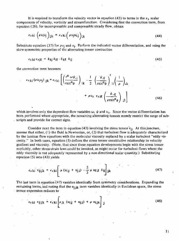
It is required to transform the velocity vector in equation (43) to terms in the x3 scalarcomponents of velocity, vorticity and streamfunction. Considering first the convection term, fromequation (26), for incompressible and compressible steady flow, obtain

e3 ki P uiUj 3.k = e 3 ki ( P ujuij \ y, (44)

Substitute equation (37) for pu; and Uj. Perform the indicated vector differentiation, and using theskew-symmetric properties of the alternating tensor contraction

jj (45)

the convection term becomes

rsina0 / ,k 2

1 \-p /,

,„ ,;3 (46)

which involves only the dependent flow variables co, \fr and u3 . Since the vector differentiation hasbeen performed where appropriate, the remaining alternating tensors merely restrict the range of sub-scripts and provide for correct signs.

Consider next the term in equation (43) involving the stress tensor TJJ. At this juncture,assume that either, (1) the fluid is Newtonian, or, (2) that turbulent flow is adequately characterizedby the laminar flow equations with the molecular viscosity replaced by a scalar turbulent "eddy vis-cosity." In both cases, equation (5) defines the stress tensor constitutive relationship to velocitygradient and viscosity. (Note, that since these equation developments begin with the stress tensorexplicitly, other stress-strain laws could be invoked, as might occur for turbulent flows where theeddy viscosity is not adequately represented by a non-directional scalar quantity.) Substitutingequation (5) into (43) yields

r 2 " 1e3ki M ("ij + uj;0 - — n u t $ 6y (47)

The last term in equation (47) vanishes identically from symmetry considerations. Expanding theremaining terms, and noting that the Uj-j^ term vanishes identically in Euclidean space, the stresstensor expression reduces to . .

eski rijjk = e 3 Ri P,k (uij + uj^) + u. uijk (48)

11

Considering equation (48) in detail, the last term can be written as

Using equation (39), obtain equivalently

(49) .

In the remaining terms in equation (48), substitute from equation (37) for the velocities Uj and'u;.Performing the indicated vector differentiations, and using the symmetry properties for alternatingtensor contractions, obtain

.k (uij + ujj) j -k -2 ,k*) -^ I

(50)

Combining equation (49) with equation (50), and expanding the last term for clarity, the stresstensor term in equation (43) becomes, in terms of vorticity and streamfunction,

' k i^ i j jk -prsma 0

•] (51)

There remains the left-hand side of equation (43) which is non-vanishing, within the assump-tions regarding the validity of i//, only for incompressible flow. For this case,

(52)

Combining equations (46), (51) and (52), the x3 scalar component of the curl of the Navier-Stokes equation (27), written entirely in terms of the vorticity, streamfunction and x3 componentof velocity u3, becomes

/ Mp ,

«,„ / J _ ) \\ prsina0 / ;3 /

Re prsmk.5 3 (53)

The form of equation (53) is desired for computational purposes, since the velocity vector andpressure have been explicitly eliminated. However, conceptual clarity results from transformation ofthe terms containing 1//4 into velocities. Contracting equation (37) with 63^ and using equation (41)yields • - " '

(547

12

Removing the \b,k the terms in equation (53), the equivalent form with velocities is

>J3 ( U j - U 3 5 j 3 ) . j

j

;k <5 5>

The convention on x3 in each coordinate system allows simplification of terms involving pu3 .For rectangular, cylindrical, and spherical coordinates, respectively, define

Xj= {x,y,0[

= lz'r'0f (56)

Then, for example, in cylindrical and spherical coordinates, respectively obtain

e3ki(PMj 3(Ui-u 36 i 3) j ) . k =p^ (pu3)*z

(57)r \ r >0 T

The x3 Component of the Navier-Stokes Equation

The determination of u3) in terms of co and i//,, is obtained from solution of the x3 componentof the Navier-Stokes equation, which is

(pU3), t = - (pUjU3) ; i - P,3 + T j j y . . (58).

assuming the body force distribution has no x3 component. The x3 derivative of pressure is includedin equation (58) to account for flow processes through "corkscrew" devices.-

Using equation (37) to replace puj and proceeding through the details of the vector derivativeof u3 , equation (58) becomes

^'i \— "3

sina0 ' ;i- />U 3 U 3 ;3 - p,3

rsinu

i I /.. .. \ 1 .. .. . .. .. i (59)

Note that u;;3 does not vanish identically. For example, in cylindrical coordinates

(60) u 3 ; 3 3 = - - u 3 (61)

For incompressible flow, the transient term may be retained; otherwise, only the steady state solu-tion is correctly specified.

The Species Continuity Equation

For multi-component flow, equation (25) describes each species mass fraction with respectto mutual convective, diffusive and reactive processes. Transformation to the desired computationalform simply involves replacement of puj by the streamfunction definition, equation (37). Since thedivergence of equation (37) vanishes, and Ya is not a function of x3, the desired equation becomes

e 3 i j i-Y" .j - pu3 Y"U + Y",: .:+Sa (62)J \rsina0 / ' \ ,/'•* \ Pr / '

The number of equations (62) equals the total number of species present, and the transient solutionis correctly specified only for species of identical molecular weight.

The Energy Equation

The form selected to express energy conservation, equation (28), is particularly well suitedfor numerical computation in the problem class being considered. The explicit pressure influence iscontained solely within the temporal dependence. Since the pressure, as an explicitly coupled de-pendent variable, has been eliminated from the momentum equations as well, solutions to steady-state problems for either incompressible or compressible flow are possible, without solution for thepressure field, provided that the implicit influence of pressure as a thermodynamic variable can besuitably approximated. This advantage is particularly noteworthy, since most numerical algorithmsfor fluid mechanics, which contain pressure as an explicitly coupled dependent variable, are speciallydesigned to "half-step" iterate between the flow field and the pressure distribution. Inefficiency ornumerical instability characterizes the attempt to march both variable types simultaneously.

To cast equation (28) into the desired computational form, replace the velocity vector by thestreamfunction definition, equation (37). The convection term becomes

l-± l + pu3 5 i3\ H (63)rsinu0 /

Using equations (5) and (6), the irreversible work term is

Using equations (37) and (41), the first right hand term becomes

14

Using equation (45) also, the second term becomes

Via =T** V

;i prsina0 \prsina0

prsina0(66)

The final term in equation (64) can be transformed using equation (26), to

uiuk;k = -uiuk£n">k

Its desired computational equivalent is

(67)

5j3 (68)

Combining equations (64) - (67), the irreversible work contribution to the energy equationbecomes

7^1-~ prsin 0)

+ —I >3prsina0

*?t p / . rsina0 rsiI'1

-2u3 e3kg l -I(69)

15

The computational form for the energy equation thus becomes

(PH),t = (Ec) p,t - - Ji H,kRe Pr

_JNk_" /'' *.j "\prsina0 \prsina0/

2 . 2u!;k -H u3 ; 3prsina0

rsina0 rsina0\ p /^

2uRePr,,

PQ (70)

For compressible flow, the time derivative terms must be set to zero. Equation (70) is valid aswritten for transient incompressible flow.

Recovery of Pressure ,

The pressure distribution is recovered from the vorticity-streamfunction characterization ofthis problem class by enforcing linear momentum conservation. Equation (27) can be transformed "to the Laplacian oh pressure by an-additional differentiation, and solved as boundary value problem.Since this is not a well-posed description for pressure, the preferable approach may be to integrateequation (27) after contraction with the infinitesimal displacement vector, dxj, yielding

Note that the left side of equation (71) is the integral of a perfect differential and thus independentof path. Hence, the pressure at any point in the field can be determined, in comparison to some re-ference value, by integration over an arbitrary (the easiest) path between the two points. Thus, theentire pressure field need not be computed to obtain selected pressures, for example, at an exteriorwall. Upon noting that the integrand in the last term of equation (71) is Xj independent, arid denotingintegrals of perfect differentials as A, equation (71) becomes

Ap = -/(puiUj) ;j dxj + -L + xb (72)

16,

To consider the convection contribution to equation (72), replace PUJUJ by equation (37).Performing the indicated differentiation, using equations (41) and (45), and noting x3 independenceof some integrands, obtain

p(rsina<>)

(73)

Ax 3rsina</> / ;

Recall that u3 -3 is transformed to equivalent terms in i// for each particular coordinate system.

The same procedures are used to transform the stress tensor contribution to computationalvariables. Integrating selected terms by parts, the following form can be obtained.

ij;jd xi prsina0 / ;j prsina0

. .' >J

dx:

Ax3(74)

Substituting equation (37) for the integrand of the time dependent contribution to equation (72),and combining terms, the following form results for determination of the pressure at any point inthe field.

17

Ap = A _i_ r/^jk^-kV 2. 63Jk^)k /_M^ [\prsina0/ ;j " 3 M isina0 \ p /

».n_L /^3 ik^>•* I Re \ prsina 4>

eii

prsina0

J_Re rsina 0

J_3t

dx;

Ax,_

Re2pu 3 : 3 (75)

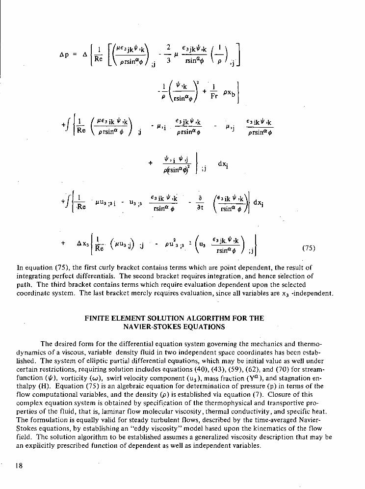
In equation (75), the first curly bracket contains terms which are point dependent, the result ofintegrating perfect differentials. The second bracket requires integration, and hence selection ofpath. The third bracket contains terms which require evaluation dependent upon the selectedcoordinate system. The last bracket merely requires evaluation, since all variables are x3 -independent.

FINITE ELEMENT SOLUTION ALGORITHM FOR THENAVIER-STOKES EQUATIONS

The desired form for the differential equation system governing the mechanics and thermo-dynamics of a viscous, variable density fluid in two independent space coordinates has been estab-lished. The system of elliptic partial differential equations, which may be initial value as well undercertain restrictions, requiring solution includes equations (40), (43), (59), (62), and (70) for stream-function (i//), vorticity (co), swirl velocity component (u3), mass fraction (Ya), and stagnation en-thalpy (H). Equation (75) is an algebraic equation for determination of pressure (p) in terms of theflow computational variables, and the density (p) is established via equation (7). Closure of thiscomplex equation system is obtained by specification of the thermophysical and transportive pro-perties of the fluid, that is, laminar flow molecular viscosity, thermal conductivity, and specific heat.The formulation is equally valid for steady turbulent flows, described by the time-averaged Navier-Stokes equations, by establishing an "eddy viscosity" model based upon the kinematics of the flowfield. The solution algorithm to be established assumes a generalized viscosity description that may bean explicitly prescribed function of dependent as well as independent variables.

18

The uniformity of the derived differential equation description for the computational de-pendent variables is evident as specific variants of the nonlinear elliptic partial differential equationof mathematical physics. Identifying q as a generalized dependent variable, the uniform descriptionbelonging to each of the equations (40), (43), (59), (62) and (70) is

N(q)5K[Kq,k];k - [e3kj - i- q] ;k + f(q,q ) k ,Xj) - g(p,q,t) = 0 (76)rsin"0

In equation (76), N(q) is the specified differential operator for q, the first right side term is theelliptic operator, the second term is the convection operator, and f and g are specified functions oftheir arguments, see Table 1 , corresponding to q identified with each dependent variable. Sinceequation (76) is elliptic, unique solutions are obtained only after specification of boundary con-ditions, the most useful and general form of which relates the function and its normal derivativeeverywhere on the closure, 3R, of the solution domain, R, as

T?(q) = aO > (Xj.t) q (xj.t) + a(2) (Xj,t) q (xj.t) ,knk - a(3) (Xj,t) = 0 (77)

In equation (77), the a(') (Xj,t) are user-specified coefficients enforcing the boundary conditionswhich may be time dependent, the superscript bar notation constrains Xj to 9R, and nk is the localoutward pointing unit normal vector. For g nonvanishing in equation (76), or for use as an esti-mated distribution to start an iteration to steady state, an initial distribution is also required; hence,assume given throughout R

q(Xj,0) = QQ(Xi) (78)

Formation of the finite element solution for the two-dimensional Navier-Stokes equationsis thus obtained by establishing the algorithm for the equation system (76) - (78) identified for eachdependent variable requiring solution. The theoretical foundation is the method of weighted resi-duals (MWR) (Reference 1) applied on a local basis. Discussion on the formulational aspects of thisalgorithm are reported for a considerably restricted problem class within the Navier-Stokes equations(References 6, 8) as well as for three-dimensional boundary-layer-type flow fields (References 7, 10).Since equation (76) is valid throughout R, it is valid in disjoint interior subdomains Rm, describedby (xj,t)e Rm x [0, oo ) called "finite elements," wherein URm = R. Form an approximate solutionto equation (76) within Rm x [0, °°), called q^ (X|,t), by expansion into a series solution of the form

= |uXi)}T(Q(t))m (79)

wherein the functionals Lk(xj) are members of a function set that is complete in Rm, and the un-known expansion coefficients, Qk(t), represent the time-dependent values of q^ (xj,t) at specificpoints called "nodes" interior to Rm and on the closure, 9Rm. Equation (79) is a scalar, the secondform introduces the column matrix notation and its transpose (superscript T), and the method ofselection of the Lk is user specifiable and problem class dependent. To establish the values takenby the expansion coefficients in equation (79), require that the local error in the approximate solu:

tion to both the differential equation (77), N(qm), and the boundary condition statement, nfarn).if applicable, that is, 3Rm coincident with 9R, equation (78), be orthogonal to the functional set in

19

zcd

B-

• ... -P ex.

3^_ E j OHi-§' S£ t*i-f*« -3 U< H wH - •< W

OS Q

' ' Z§0

:. C 3 p .

., ^^."" ' & f a -

uJ ; -

IS

. 3a-w

trQ.

o-Q.

CL

gV

a

i

• <u : <u I; oi -J 1

or-

20

equation (79). This is accomplished by enforcing the local variant of the Galerkin criterion ofclassical MWR, that is, premultiplication of equations (77) and (78) by the approximation functional,Lk(xj), and integration over the respective domains. Employing a Lagrange multiplier, X, these

/ 3 0 (80)

The number of equations (80) is identical to the number of node points associated with the finiteelement, Rm, that is, the number of elements in the column matrix {Q(t) ) m.

Equation (80) forms the basic operation of the finite element solution procedure. Establish-ment of the global solution algorithm, and determination of X, is accomplished by evaluating equa-tion (80) in each of the m finite elements of the discretized solution domain, R, and assembly ofthese Mxn equations into a global matrix system by Boolean algebra. The rank of the global systemis less than Mxn by connectivity of the finite element domains as well as by enforcement of thoseboundary condition statements on 3R where a(2 ), equation (77), vanishes identically. Determinationof A is accomplished by observing that the lead term in equation (76), when incorporated into equa-tion (80), can be integrated by parts; alternatively, using the generalized divergence theorem (Appen-dix A), obtain

L(Xj) ) K[Kq^ J dr = K L(xj) Kq^ nkda' - * L(xj) ) ,kKq^ drm ; °Km Km

(81)

On those portions of the closure 3R coincident with 9Rm, equation (81), the corresponding segmentof the closed surface integral will cancel the boundary condition contribution, equation (80), byidentifying X with K of equation (76) and a(2) with the generalized diffusion coefficient, K. FromTable 1 , for the Navier-Stokes equations, K typically involves the Reynolds number and a'2 ) is theviscosity, ju , . except for the vorticity-streamfunction compatibility equation (40), where they areunity and inverse density. The contributions to the closed surface integral, equation (81), where3Rm is not coincident with 3R remain for evaluation. Hence, combining equations (77) - (81), theglobally assembled finite element solution algorithm for the .representative elliptic partial differentialequation system description for the Navier-Stokes equations becomes

da + R

(82.)

Using Boolean algebra as the assembly (summation) operator, the rank of the global matrixequation system (82) is identical to the total number of node points within the solution domain R,and on the closure 3R, at which the dependent variable requires solution. Equation (82) is eithera first-order ordinary differential, or algebraic equation system dependent upon whether g, equation(76), vanishes identically. In either event, the equation system is large order and the matrix structure

21

is sparse and banded about the main diagonal, with bandwidth a function of both selected discreti-zation and the order of the employed approximation function, equation (79). Solution of thealgebraic system can be obtained by many procedures including direct inverse, Gauss elimination, andequation solver techniques, for example, banded Cholesky. If the equation description is ordinarydifferential, solution is obtained using either an explicit or implicit numerical integration algorithmfor an initial value problem.

FINITE ELEMENT MATRIX GENERATION

Implementation of the finite element theory into a computer code involves assembly ofEq. (82) for the required dependent variables, hence evaluation within each element of the discre-tized solution domain. The vast experience in structural mechanics has proven the viability of trun-cated power series as approximation functions. Highly tailored finite elements have been establishedfor specific problem classes in elasticity. But for now, the use of finer discretizations using linear(simplex) approximation functionals, Eq. (79), appears'useful for the broader problem class. Theintrinsic finite element shapes for one-, two, and three-dimensional spaces, spanned by simplexfunctionals, are the line, triangle, and tetrahedron. The preferred orientations for these elementsin a local coordinate system are shown in Figure 1.

Accurate determination of the element matrices of Eq. (82) is mandatory, and involves evalu-ation of various-order moment distributions over the domain of the finite element. A straightforwardapproach involving numerical matrix multiplications, after definition of a transformation matrix(Reference 8), is generally adequate for linear equations; however, it has proven highly susceptible toaccumulated round-off for the explicitly nonlinear matrices common to the Navier-Stokes equations.An alternate approach has been developed which expands upon the natural coordinate functiondescription for finite element solution of the energy conservation equation (Reference 11). Thesefunctionals, which are an adaptation of the area coordinates of structural mechanics (Reference12) are a linearly dependent set of normalized functions that are orthogonal to the respective closuresegments of the finite element domain. For an n-dimensional space, there are n+1 simplex naturalcoordinate functions. Table 2 contains the implicit definition of these functions in their respectivespaces. (The three-dimensional descriptions, while inappropriate for the particular Navier-Stokesequation system being studied, are included to complete the finite element theoretical foundationfor future reference.) As the direct consequence of the definition, the natural coordinate functionsvanish at all node points of the finite element except one where the value is unity. Hence, thesefunctions are the elements of the approximation function column matrix, j L ) , Eq. (79). Ofparticular impact for solution of the Navier-Stokes equations is that integration of arbitrary-orderproducts of scalar components of the j L } ,.over the domain of the finite element, are analyticallyevaluable in terms of the exponent distribution, Table 3, the determinant of the equation systemdefining the Lj, Table 2, and the dimensionality of the space of the problem.

It remains to evaluate the solution algorithm, Eq. (82), for the Navier-Stokes equations usingthe natural coordinate function description, which involves matrix formation over one- and two-dimensional finite elements. (The one-dimensional element is needed to evaluate the domain closureintegrals of the solution algorithm.) The evaluations are presented for the two-dimensional flow of afluid with arbitrary density and viscosity distribution, and the axisymmetric flow of a constant prop-erty fluid. Additional integrations by parts have proven useful for the functions f(q), Eq. (76), andthe mathematical consequences of these operations are established in Appendix B.

22

Figure la. One Dimensional Space Figure Ib. Two-Dimensional Space

*3

Figure Ic. Three-Dimensional Space

Figure 1. Intrinsic Finite Element Domains for Simplex Approximation Functions

23

TABLE 2IMPLICIT DEFINITION OF SIMPLEX NATURAL

COORDINATE FUNCTIONS

Dimensions

1

2

3

Element

Line

Triangle

Tetrahedron

Nodes

2

3

4

Natural Coordinate Definition

r. ou,LX, x2J (L2

"i 1 rXj X2 X3

Yl Y2 Y3

1 1 1X, X2 . X3

Yl Y2 Y3

^1 ^2 ^3

HI(LI) (1)I < =) l(L3J (v)

1 "X4

X4

Z4

M CM1-2 = *

)L3 / \y

( Uj z )\ • / \ /

TABLE 3INTEGRALS OF; NATURAL COORDINATE FUNCTION

PRODUCTS OVER FINITE ELEMENT DOMAINS

Dimensions

1

2

3

. Integrals*

IR ' 'f1"1" nl + n2 )!

/ ni n? n^ i ni ln^lni !1 i i i J ,i. .1. . n '1 Lj L2 L3 dxdy U ••••• —/P (n+ni +n2 + n3)!

1 ^1 *^2 ^3 ^4 ^1 ^ 2 • ^1 • -^4 •I I I I I rlvrlurli — n ; .

,/p (n+ nj +n2 +n3 +n4)!

* D = Determinant of coefficient matrix defining the

natural coordinate system, see Table 2.

n = Dimensionality of the finite element space

24

Planar Finite Elements for the Two-Dimensional Navier-Stokes Equations

With the advent of the natural coordinate function description for the finite element approxi-mation functions, matrix evaluation is straightforward. Moment generation is invariant under bothcoordinate translation and rotation in Euclidean space spanned by a rectangular Cartesian basis,(Appendix C). All computations are formed in the local (primed) coordinate system, Figure 1 ,defined by the tensor transformation law

x'j = aijXj + rj (83)

where rj is the position vector to the origin of the primed coordinate system, and the ay are thedirection cosines of the coordinate transformation. The integration kernels for two-dimensionalspace, Eq. (82), are

dr = tmdx', dxi (84a) da = tmdx', (84b)

where tm is the thickness of the m^n finite element. (Variable element thickness allows solution ofpredominantly two-dimensional flows in irregular depth channels, for example, rivers.) Since nodifference exists between differentiation of scalars and vectors, the semi-colon operator reduces tothe comma. Furthermore, no u3 velocity component can.exist in rectangular Cartesian space.

All expressions but the third, Eq. (82), are standard for all dependent variables. For thegeneralized diffusion term, using Eq. (79) for both qm and the generalized diffusion term, Km, andtransposing scalar quantities, obtain

|B10| [B211S]JQ} m (85)

The standard matrices, as used in Eq. (85) and the following, are defined in Table 4. If JQ} in Eq.(85) is identified, for example, with vorticity, then K~I equals the Reynolds number, Re, and the

elements of j K } m are the element node point values of viscosity, ju. The second term of Eq. (82),which accounts for convection processes, becomes

m

= |B10| H.T [B211A] {Q} m (86)

Equation (86) is eligible for integration by parts; however, no arbitrariness exists for its evaluation,Appendix B, so no benefit accrues from that operation. In contra-distinction to this, the contribu-tions to Eq. (82) stemming from the final term, involving a closed integration on 3Rjn, are non-vanishing for all Rm> but can be made to cancel in pairs upon Boolean assembly of the global algor-ithm, see Appendix B. Hence, the sole surface integrals requiring evaluation occur when dRm and 3Rare coincident, and a^1 ' and/or am'3 ' are non-vanishing. Therefore, the only contribution to Eq.(82), from all surface integrals, reduces to two terms,

25

TABLE 4

STANDARD FINITE ELEMENT MATRIX FORMS FOR SIMPLEX FUNCT1ONALS INTWO-DIMENSIONAL SPACE

MATRIXNAME< ! )

IB200S)

[B21 IS]

[B2I1A]

( A m l1AIOI

MATRIXFUNCTION

f{ (L| {t}TdT

JRKm

I.I 1, 1 TIM'k 'LI • k

T

JRKm

/ JU lUTdo1 JL} JLJ do

/ 111 .,„}L( do

MATRIX EVALUAT1ON(2)

("2 1 l] <3>

p -1 0]/ 1 \2 , nlx,p,')\X1P2/ L Oj

/X2P3 V 2 X2P3 /X2P3 \ /X2P3 \\X1P2 / ' XIP2 \X1P2 /' \X1P2 /

J ' f /X2P3\ 2 /X2P3\\X2P3 / ' \x m) • \x\P2)

, 1

" [o -i r-i- , 0 - 1 .2A -i i o

Amtm ( ' )3 (!)

t~i

2 1 0 1* * J2 : J2 )' j

(1) Matrix names are a 6 digit code covering dimensionality, nonlinearity, degree ofdifferentiation and special matrix properties, as [a, b, c, d, e, fj where:

a = A, B, C for spaces of one-, two-, and three-dimensions,

b = number of natural coordinate functions appearing in integral or matrix,

c, d, e = (0, 1) Boolean counters indicating (no, yes) differentiation of each function,

e or f = S, A, A for matrix symmetric, antisymmetric or general.

(2) Am = 'A (XIP2) (X2P3), the plane area of the (triangular) finite element, where thefour digit codes signify node point coordinates in the primed system, for example,

XIP2 = the X! prime coordinate of node 2,

X2P3 = the x, prime coordinate of node 3,

tm _ average thickness of the finite element,

Sm = length of side along which the boundary condition isapplied (=X1P2)

(3) Symmetric matrices are written in upper triangular form.

26

IM am( l)1rndo = KaJO [A200S] |Q}m (87)

l L }a m ( 3 >da = Kam(3)|A10} (88)

where the am are user-supplied boundary condition constraints.

One more standard matrix exists should the analysis be performed for the transient motion ofan incompressible fluid, that is, hydrodynamics. The function gm, Eq. (82), is non-vanishing for alldependent variables excepting streamfunction. The numerical evaluation for vorticity and massfraction takes the form:

W £> = / |L) pm \L\ T £{Q(t)} mdr = pm [B200S] (Q(t)} 'm (89)m Rm

In Eq. (89), the superscript bar signifies an element-averaged value for density, while the primedenotes that the dependent variable matrix contains the time derivatives of the node pointvalues of the respective functions. Hence, in this case, Eq. (82) is a system of ordinary differ-ential equations. For the energy equation, a more convenient form exists in terms of temper-ature as the time dependent variable. Hence, obtain

m

'm[B211S] |*}.'m (90)

Since the mechanics and thermodynamics of incompressible flow are separable, I\M 'm can be in-dependently evaluated using a finite difference formula for the derivative of a tabulated function.Thus, the second term in Eq. (90) is at most a source term, usually of negligible magnitude, sincethe Eckert number is typically small for the more common incompressible flow configurations.

Several additional matrix evaluations are required for fm to complete the description ofEq. (82) for specific dependent variables. Taking them in the order of occurrence in Table 1 (fm isthe approximation to fin Rm), for streamfunction, the second term simply cancels the convectionoperator of the standard equation form, Eq. (82). For the remaining term, obtain

/R |L}o,mdr = [B200S] \n \ m (91)

For solution of vorticity, the terms involving u3 are discarded, and the remaining terms can beeffectively integrated by parts to render the forms more tractable. Considering the density term, con-tributions stemming from the resultant surface integral can be made to vanish in pairs on all 3Rm inte- -'rior to 3R upon assembly of the global algorithm, as discussed in Appendix B. For locations where

27

3Rm coincides with 3R, no arbitrariness exists for evaluation of the surface integral. However, 3Rcoincides with \l> equal to a constant everywhere except at mass flow injection points. At theselocations, the density may usually be assumed constant, and either condition is sufficient to renderthe matrix identically zero. So, the sole term requiring evaluation is

[B211S] j i / / ( m [ B 2 1 1 A ] \ - p \ m (92)

where p"1 is selected as the preferred primative computational variable due to its universal appearance.Thus, the elements of j-Ll are the inverse of the node point densities of Rm.

JT1

After integration by parts of the viscosity gradient terms, no surface integral evaluations oninterior 3Rm are required, based on the analysis used for density. For those segments of 3Rm,coincident with 3R and for no mass injection, the flow is laminar, hence viscosity is only weaklytemperature dependent. At injection points, the density may be assumed constant, and either con-dition renders the surface integral terms identically zero. So, for variable viscosity, the sole contri-buting terms from fm for vorticity become

[B211S] {M}

(93)

m

mum

where the elements of the column matrix |/i) are the node point values of viscosity.

The sole term in fm for the species continuity equation is that due to sources of mass. Thisterm could be conveniently expressed as either element or node point dependent. The respectivematrix forms are,

|L} Sadr = Sm|B10} (94a)Rm

= [B200S] |Sa|m (94b)

For energy conservation, Eq. (70), the entire viscous dissipation term may be integrated byparts, and the resultant surface integrals on interior 3Rm vanish in pairs upon assembly and renderedzero on exterior surfaces. The various terms are combined to yield the following form

Rm

| [ B 2 1 1 S ] { } m [ B 2 1 1 S ] |^}m{M}mfB200S] ( [ m (95)

28

Finally, the source term, pQ,.in the energy equation would typically be node point dependent;hence

(L}pQmdr = [B200S] {pQ}m (96)Rm

It remains to establish the boundary condition specifications, at-1', Eq. (77), for thederived dependent variables, streamfunction and vorticity, in terms of known velocity anddensity distributions. The practical engineering specification is velocity scalar components per-pendicular and parallel to the domain closure 3R, and mass flux across appropriate closuresegments. The closure specifically need not be, and oftentimes is not, parallel to coordinatesurfaces of the global reference frame. Establishment is straightforward; contracting Eq. (37)with an alternator, and using Eq. (41), obtain

1— l//,u = e,:i,U: (97)p K 1K '

Referring to Figure Ib, identify the surface between nodes 1 and 2 of Rm as coinciding witha segment, 3Rm, of 3R whereupon a specified velocity and mass flux distribution exists. Assumethe velocity scalar components perpendicular (u^) and parallel (un) to the line are assigned ateach node point. Contract Eq. (97) with an infinitesimal displacement vector tangent to 3Rm

and integrate to obtain(2) (2) (2)

X' 1 ' Xl i *1 /

P J '~ Jo • o o

Using Eq. (79) for all variables, the integrals are directly evaluable, Table 3; hence for a spec-ified normal velocity on 3Rm, the equivalent streamfunction constraint is

(2) (i) g"1!"1 ' +u12)m

ill = W •*• - -"m ~m

G +(;)P'

Equation (99), in combination with the normal mass flux specification, determines both J/ and

— on 3Rm. In Eq. (99), Uj^ is defined positive for mass efflux from Rm, and £m is the length

of the closure segment between nodes 1 and 2.

The counterpart evaluation of Eq. (97), contracted with the outward pointing unit normalvector, n^, becomes

= e3ikuink = -u|| 000)

29

where UN is defined positive for alignment parallel to the x'^axis, Figure Ib.the equivalent stream function boundary condition constraint becomes

m

O)am

= "UN

= 0

Using Eq. (77),

(101)

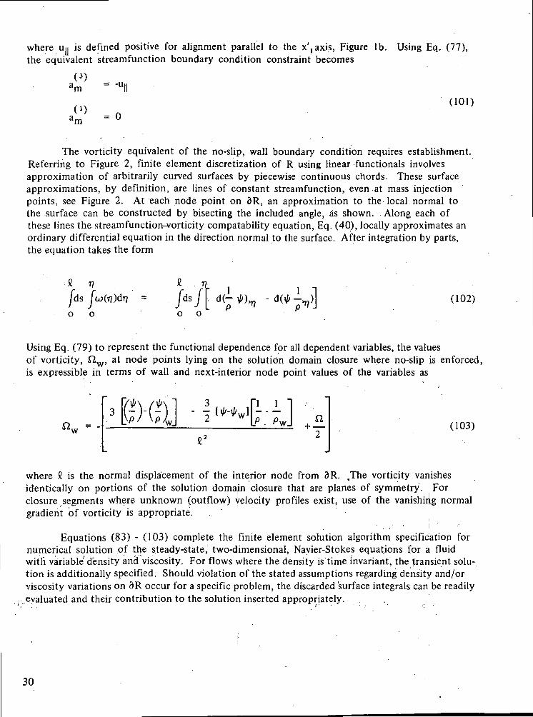
The vorticity equivalent of the no-slip, wall boundary condition requires establishment.Referring to Figure 2, finite element discretization of R using linear functional involvesapproximation of arbitrarily curved surfaces by piecewise continuous chords. These surfaceapproximations, by definition, are lines of constant streamfunction, even at mass injectionpoints, see Figure 2. At each node point on 3R, an approximation to the local normal tothe surface can be constructed by bisecting the included angle, as shown. Along each ofthese lines the stream fun ction-vorticity compatability equation, Eq. (40), locally approximates anordinary differential equation in the direction normal to the surface. After integration by parts,the equation takes the form

£ 17

dsf

(102)

Using Eq. (79) to represent the functional dependence for all dependent variables, the valuesof vorticity, £2W, at node points lying on the solution domain closure where no-slip is enforced,is expressible in terms of wall and next-interior node point values of the variables as

"w = -

3 ~ - -w_

(103)

where £ is the normal displacement of the interior node from 3R. .The vorticity vanishesidentically on portions of the solution domain closure that are planes of symmetry. Forclosure segments where unknown (outflow) velocity profiles exist, use of the vanishing normalgradient of vorticity is appropriate.

• . .• • • lEquations (83) - (103) complete the finite element solution algorithm specification for

numerical solution of the steady-state, two-dimensional, Nayier-Stokes equations for a fluidwith variable density and viscosity. For flows where the density is time invariant, the transient solu-tion is additionally specified. Should violation of the stated assumptions regarding density and/orviscosity variations on 3R occur for a specific problem, the discarded surface integrals can be readily.evaluated and their contribution to the solution inserted appropriately. , .

30

xl

Figure 2. Establishment of Vorticity Boundary Condition Statement

Planar Ring Finite Elements for the AxisymmetricIncompressible Navier-Stokes Equations

In axisymmetric space, moment generation is invariant only under coordinate rotation, seeAppendix C. The preferred element orientation remains in the primed coordinate systems, Figure 1,as defined by Eq. (83). The integration kernels become, Tespectively,

AT = 27rx2dxJ dx2

da = 27ix2dx{.

(104a)

(104b)

where x2 is the radial coordinate in the global reference frame of a point in Rm. Before integrationscan be performed, it is necessary to express x2 in the primed system; using Table 2 obtain

x2 = (105)

where x/1' is the radial coordinate of node point 1 in the global reference frame.

The finite element counterpart of the'generalized diffusion term, Eq. (82), now requires addi-tional consideration for streamfunction. Since the diffusion coefficient contains a metric coefficient,Table 1, the resultant differential operator is not the Laplacian in cylindrical coordinates. The explicitappearance of a Laplacian can be extracted by definition of a new variable, <t> = \l//x-2' whereupon thecompatibility equation, Eq. (40) takes the form

(106)

For the function 0, as well as the remainder of the dependent variables, the generalized diffusion termfor constant density and viscosity takes the form

31

= K/|LJ ^K™ {LjT^ {Q |mdr

B10| [B211S] |Q( m (107)

where Km is an element scalar stemming 'from the assumed constant properties, the elements of {RJ m

are the node radial coordinates in the global reference frame, and in axisymmetric space, the elementthickness tm defined in j BIO} , Table 4, is replaced by 2n. ,

The convection matrix becomesi//*.

f |L l«3ki— qnVr = / l L H * l ^ | L } , e 3 k i | L » T |Q | m dx ldx ijRm *2 " Rm

= { B I O } U}^[B211A] |Q}m . (108)

which is identical to the two-dimensional form with tm replaced by 2tr. The boundary conditionmatrices for the dependent variables are

i L ) a m U ) < l m d f f = KamO)[A200SA] J Q J m (109)m

K[ JL}am( 3 )da = Kam ^ JAIOA) (110)

In Eqs. (109) - (1 10), the suffix A in the matrix name refers to the axisymmetric counterpart of thestandard form, see Table 5. In each case, the first term is identical to the two-dimensional form withtm replaced by 2ir.

The transient algorithm is correctly specified for constant density flows. The axisymmetricfinite element evaluation for g , Eq. (82), becomes

7 ,- Rm

= pm[B200SA] (Q(t)|m (111)

The added complexity of the [B200SA] standard matrix, Table 5, stems from lack of translationalinyariance.

'' ' The sole source terms requiring evaluation. for constant property axisymmetric flows are inthe modified streamfunction equation, Eq. (106). For the vorticity term, obtain

a • (112)

Rm' ' • . ' - - ' . • - ' . - -

32

TABLE 5ADDITIONAL STANDARD MATRIX FORMS FOR SIMPLEX FUNCTIONALS

IN AXISYMMETRIC SPACE

MATRIXNAME

[A200SA]

{AIOA}

[B200SA]

FB200SCJ

MATRIXFUNCTION

r i, M . I T3Rm

/ W da9Rm

f JUJU T rRm

Rm L L CdT

MATRIX EVALUATION^1), (2)

^(

^(

^Slj

^

^

k

" I1! +(o)

!" [' ' •"2rj + r2

ri + 2r2

rl + r2

+ -2-y

-J

r^-i+ ~

+ r3+ r3+ 2r3^

p

'i.0

\

3 . 0

°V

)"2 2 "

6 22.

p. 1 2l\

. a -2 j )

(1) The lower case r refers to node radial coordinates in the global reference frame.

(2) Symmetric matrices are written in upper triangular form.

(3) fB200SCj is a diagonal matrix.

For constant density, the form for the remaining term is

( i L H L | T M m 4- dr-J 1 j i ' I J U1 px" 2

3

Rm

where [B200S] is the rectangular Cartesian matrix defined in Table 4 with tm replaced by 2?r. Theboundary condition statements for both streamfunction and vorticity are identical to the two dimen-sional specifications, with the addition of respective inverse node radii to the denominator ofEq. (99) and the numerator of Eq. (103).

33

COMOC COMPUTER PROGRAM ;

The COMOC (Computational Continuum Mechanics) general-purpose computer programsystem embodies the derived finite element solution algorithm for the general initial value, ellipticboundary value equation system, and is coded entirely in terms of generalized non-dimensionalindependent and dependent variables. In addition to producing the results to be discussed, it hasbeen'exercised for problems in transient heat conduction (Reference 11) and the three-dimensionalboundary layer equations (References 7 and 9). The program consists of four basic Modules.In the INPUT Module, the desired discretization is formed by specification of the plane coordinatesof-the triad of vertex nodes for each finite element. The non-vanishing boundary conditioncoefficients am' , Equation (82), are included as element information for each dependent variableto be solved, since in general the different Q's have individual specifications. The next two Modulesare basically DO loops on the finite elements of the discretization. In the GEOMETRY Module;the element standard matrices are formed and stored. The INTEGRATION Module embodies theintegration algorithm for the system of ordinary differential equations as well as access to an algebraicequation system solver. For either case, the basic element operation is formation of Eq. (82), andassembly of the element matrices into the global representation. The integration algorithm presentlyused by COMOC is an explicit, single-step, multi-stage finite difference procedure with a large regionof absolute stability (Reference 11). A banded Cholesky equation solver is used for the algebraicsystems. At user-selected points, the OUTPUT Module is called to record the arrays within thedependent variable vectors (Q } and other desired parameters.

NUMERICAL RESULTSj

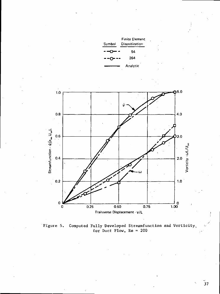
Numerical evaluation of the finite-element solution algorithm for the two-dimensional Navier-Stokes equations, as embodied in the COMOC computer program, has been performed to assess solu-tion accuracy, convergence, and versatility of the finite-element concept. A problem of particularvalue for accuracy studies is developing flow in a rectangular duct of an isothermal constant-densityfluid. This problem retains the full nonlinear character of the Navier-Stokes equ3nons,;and the out-flow boundary conditions of vanishing normal gradient for both stream function and'vorticity areanalytically exact for sufficient duct length. Figure 3 illustrates the basic 144 finite element discreti-zation of the duct flow problem; for Re = 200, based on duct width, the fully developed velocity flowfield should be attained within the duct (Reference 13). Additional discretizations studied havedoubled and halved the number of node rows, and doubled the number of node columns; these arereferred to, respectively, as the 264, 54 and 276 finite element discretizations. Figure 4 shows theCOMOC computed velocity distributions at the terminal node column of the solution domain for thefour studied discretizations. Since velocity is a constant within an element for linear streamfunctionapproximations, Equation (37), the velocity contours are correspondingly constructed. For all dis-cretizations, the analytic solution approximately bisects the computed constant velocity within eachelement, and convergence with discretization is illustrated. Within the constraint of element constantvelocity, solution accuracy is generally good for all discretizations, although refinement of the gridcertainly improves the solution for points not coincident with an approximate element centroid.Poorest improvement in accuracy occurs near the duct centerline where the 2.5% inaccuracy of the264 element solution is modestly poorer than either the 144 or 276 element solutions. It is recalledthat the 264 element solution doubles the node rows only, which yields element aspect (length/width)ratios of about 50 in this region. Propagation of vorticity to the duct centerline is consequential onlyfor x/L > 8.0, and its underprediction in the far downstream region is reflected in the lack of comput-ed velocity improvement. This is illustrated further in Figure 5 which presents computed streamfunc-

34

,C o

p8 .o d

OJ

ro

H 8

0.0) I.Z5 2.SO ».7S 5.00 «.ZS 7.SO ».7S 10.00 11.s I2.SO IJ.H 11.03 IS. a 17.il 11.75 29.00 H.2S

Longitudinal Coordinate - x/L

Figure 3. Discretization of Rectangular Duct into 144 Triangular Finite Elements

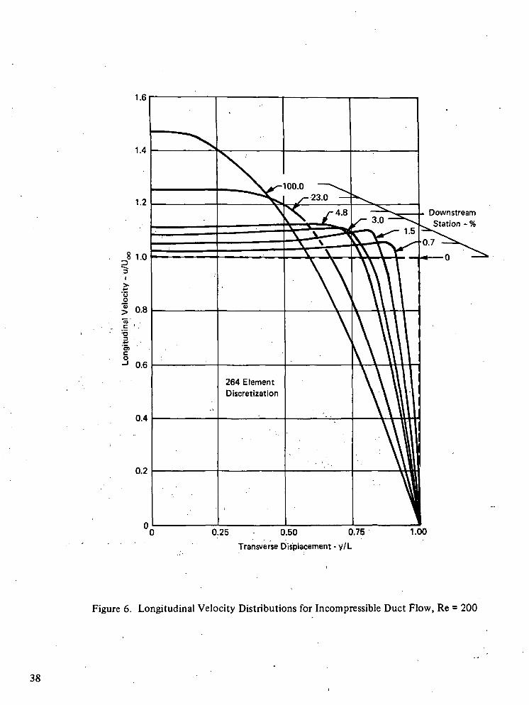
tion and vorticity in comparison to the analytic values. The improvement in computed vorticity withdiscretization is also illustrated, and the nodal .accuracy of the 54 element streamfunction solution isremarkable and reflects the well-posedness of streamfunction cast as a boundary value problem. Figure6 illustrates computed longitudinal velocity contours at various stations downstream of the duct inletfor the 264 element discretization. Velocity overshoot is predicted to occur over the first 4.8% ofthe duct length and is maximum at the 1.5% length station. The magnitude and location of velocityovershoot is in agreement with other solutions of the same problem (References 12, 14).

Solution accuracy, as well as computational speed for a transient problem, depends not onlyupon discretization but also upon the manner selected for assembly of the finite-element equivalentof the function, g, Equation (82). Initial value integration algorithms are typically derived for or-dinary differential equation systems that are explicitly uncoupled in the derivatives; that is, thestandard form is

{Q}' = f( |Q| , t ) (114)

Global assembly of the finite element solution algorithm, Equation (82), produces a transient equa-tion description wherein the derivatives are explicitly coupled by the [B200S].or [B200SA] finite-element matrices. Hence, Boolean assembly of the transient term yields a global description thatcontains a sparse symmetric matrix banded about the main diagonal modifying the { Q } ' matrix.The bandwidth is a function of discretization, and premultiplication of the entire equation system byits inverse (or equation solver equivalent) is needed to achieve the required form, Eq. (114). Theinverse is symmetric and a full matrix. Thus, this operation couples the time varying behavior ofnode point dependent variables to all nodes of the discretization. The inversion process can be madetrivial, and nearest-neighbor transient behavior maintained, by "condensing" the elements of the[B200S] and [B200SA] matrices, on rows, which fenders the global matrix diagonal. In two-dimen-sional space, this operation is a simple averaging, see Table 4. In axisymmetry, the geometry of thediscretization and lack of translational invariance produces the condensed matrix form listed as[B200SCJ in Table 5.

35

1.6 r-

Fmite ElementDiscretization

1 54144,276

264Analytic

0.25 0.50 0.75Transverse Displacement, y/L

1.00

Figure 4. Computed Fully Developed Longitudinal Velocity Distributions, Re = 200

36

Finite ElementSymbol Discretization

--O-— 264

———— Analytic

0.25 0.50 0.75

Transverse Displacement - y/L

1.00

Figure 5. Computed Fully Developed Streamfunction and Vorticity,for Duct Flow, Re = 200

37

264 ElementDiscretization

0.25 0.50 0.75

Transverse Displacement • y/L

1.00

Figure 6. Longitudinal Velocity Distributions for Incompressible Duct Flow, Re = 200

38

Both the consistent and condensed forms for the initial value matrix have been evaluated fortransient problems by COMOC. Employing the consistent form produces a significantly "stiffer"ordinary differential equation system as manifested by the small integration step-size accepted'byCOMOC. Solution accuracy appears generally acceptable except for spurious behavior during impul-sive starts in regions of initially uniform variable distributions. For uniformly positive fluxes intothese domains, wave-like depression of selective node point values below their initial values is observ-ed. Evaluation of this phenomenon, and absolute assessment of solution accuracy was made bystudying the heating of a quiescent fluid in an axisymmetric duct subject to external uniform heatingfrom the wall. For this problem, the flow equations are identically satisfied, and only the energyequation (70) requires solution after deletion of both the nonlinear source term, Equation (90), andthe convection term. Figure 7 shows a comparison between COMOC computed radial temperaturedistributions in the fluid, for two discretizations and both assembly options for the initial valuematrix, and an analytic solution (Reference 15). At the outer wall,—= 1, solution accuracy for therocoarse discretization and consistent matrix assembly is excellent. The depression below the initialuniform temperature at the interior radii nodes is illustrated to propagate into the interior region.The solution accuracy for the same discretization using the condensed matrix form, is noticeablypoorer at the wall, and although devoid of the depressions is only a local improvement elsewhere.However, doubling the discretization and employing the condensed form produces a comparable oruniformly more accurate solution everywhere.

',' .,•'' ,

For small-scale problems involving less than about 50 finite elements, experimentation indi-cates that computer CPU execution time for double discretization and condensed form solutions isabout equal to the corresponding consistent form solution. Even though the consistent form inversecan be stored, for larger problems, the lengthy multiplication process coupled with lower stabilityproduces execution times uniformly in excess of the corresponding.condensed, double-discretizationsolution. Hence, until integration algorithms for equation systems that are explicitly coupled in thederivatives are developed (for example, see Reference 16), it appears uniformly preferable to employfiner discretizations and the condensed matrix form for solution of transient problems by finiteelement techniques.

Abrupt non-uniformities in discretization near a no-slip surface of the domain closure havebeen observed to adversely affected solution accuracy, primarily through the vorticity boundary con-dition statement, Equation (103). Evaluation of solution deviations was accomplished using variationsof the duct flow discretization, Figure 3 after removal of the row of nodes at y/L = 0.95. The analyticsteady-state vorticity distribution was uniformly applied across the entire duct length as the initialcondition. The affect on computed streamfunction accuracy, of sequentially replacing nodes alongthe line y/L = 0.95, starting from the left, is illustrated in Figure 8a. At each abrupt change in dis-cretization, the streamfunction alternately over- and under - predicts the correct value by less thanabout ± 0.5%. This variation in streamfunction accuracy is probably acceptable for most practicalflow field predictions. However, near a no-slip wall, these minor errors in streamfunction canproduce an extremely large error in wall vorticity, as computed through Equation (103) and illus-trated in Figure 8b. In all cases, continuing the transient solution from these initial computationsproduced convergence to the correct solution for both streamfunction and vorticity. The directionof the diagonals of elements near a wall did not materially affect solution accuracy as long as theywere all of the same slope, that is, positive or negative. However, Figure 9 shows that alternatingthe slopes has a detrimental effect on computed streamfunction accuracy. As also illustrated, finerdiscretization improved solution accuracy. This evidence indicates that regular and uniform dis-cretizations near a no-slip wall are preferable.

39

SymbolRadial

DiscretizationInitial Value

Matrix

5 Consistent5 Condensed

10 CondensedSeries Solution (Ref. 15) —

1.10

1.08

1.06

I

&

I

1.04

1.02

1.00 hr

0.98 l

— = 1.0

>• — = 0.9

-=0.7

200 400Solution Time (sec)

600

Figure 7. Computed Transient Temperature Distribution inAxisymmetric Quiescent Duct

40

o

5a

oc3

£+•*CO

o

Q -50

;U

O

-100

8(a) Streamfunction Solution- '*

DiscretizationChange - x/L

10 15Longitudinal Station - x/L

8{b) Vorticity Solution

Figure 8. Discretization Influence on Vorticity and Streamfunction Near a Wall

41

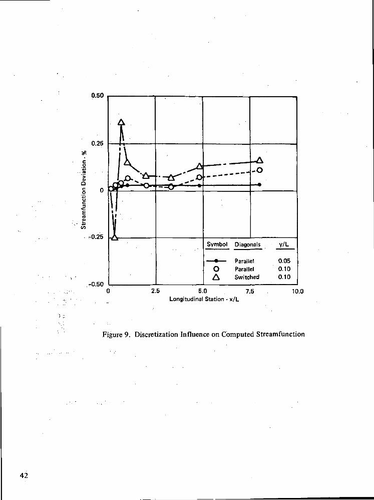
0.50

0.25

sR

o*

0>O

o|

**—

CO0)

-0.25

-0.50

!N.Jr^^

\t 'Iu

••-£s^"' o--O~ *

- . -

> » ^ ^

-A

-O

Symbol Diagonals y/L

— •— Parallel 0.05O Parallel 0.10A Switched 0.10

2.5 5.0 7.5Longitudinal Station - x/L

10.0

Figure 9. Discretization Influence on Computed Streamfunction

42

A crucial analysis for the class of flows governed by the full Navier-Stokes equations is pre-diction of regions of recirculation imbedded within an arbitrary flow field. For example, it isprecisely this phenomenon that prevents use of boundary layer theory in regions of separation inotherwise predominantly boundary layer flows. A great deal of laboratory and numerical experi-mentation has been conducted for the sample geometry illustrated in Figure 10, which is flow in aduct with a considerable enlargement in cross-sectional area. The fluid will not turn the corner,but instead provides a smooth area transition by self-generation of a recirculation region. Finitedifference numerical solution procedures for this problem typically require special handling of thecorner region to promote generation of the recirculation zone (References 14, 17). There is nosuch requirement for the finite element algorithm and all wall-node vorticities are computed in auniform fashion. Of critical importance for accurate computational representation of this problemis prediction of the points of attachment of the streamline dividing the recirculation region from themain flow, both at the step and at the downstream reattachment point, points A and B, Figure 10.For flow Reynolds numbers based upon step height larger than 20 (Reference 17) the attachmentat the step occurs just below the corner on the vertical face. The downstream attachment point isapproximately linear with Reynolds number in the range 20 < Re < 200 (Reference 18). The pointsof attachment are identified by a vorticity sign change, and the stream function solution mustnumerically bifurcate to predict recirculation.

(Symmetric)

//////ss//////////s//////

Figure 10. Flow Over a Rearward Facing Step ii i •i i

The finite element solution algorithm, as embodied in COMOC, has been assessed to; accuratelypredict the rearward step steady-state- flow field for Re = 200, treating the problem as transient.Shown in Figure 11, is the finite element discretization employed for the problem. The descriptionemploys 211 finite elements and is non-uniform to gain definition in the corner region. Figure 12shows computer-generated plots of computed streamfunction and vorticity distributions (upper andlower half planes) at various time stations in the transient solution. Figure 12a presents the essen-tially inviscid starting solution corresponding to impulsive application of a pressure gradient to aquiescent, fluid-filled duct. In Figure 12b, the streamfunction contours have drawn away'from thestep base and the resultant separation bubble is detected. This bubble rapidly proceeds up the stepface, Figure 12c, and then proceeds to grow in strength and size, Figure 12d. Figures 12e - 12h pre-

43

-0.50 Q.n 2.00 J.Z5 t.SO S.TC 7.00 B.Z5 ft. SO 12.00 IS.J5 K.SO 1S.1S 11.00 U.B !».» B.TS

Longitudinal Coordinate - x/L

Figure 11. Discretization of Rearward Facing Step in a Rectangular Duct into211 Triangular Finite Elements

sent growth of the recirculation region to an essential steady-state solution. Note in each figure thepredicted occurrence of a second recirculation region at the base of the step. Within this region, theflow field corresponds to flow into a forward facing step, and the fluid again shields itself fromabrupt changes in cross-sectional area by self-generation of smooth transitions.

The point of reattachment of the dividing streamline for essential steady state, Figure 12h is.,about 2.1 step-heights downstream. This prediction agrees within 10% of an extrapolation of datapresented in Reference 18 for two-dimensional flows and with the computations of Reference 19.for axisymmetric flow. No other numerical solution to the two-dimensional rearward step prob-lem at this Reynolds number is published; further, Dorodnitsyn (Reference 18) observed thatseveral independent solution techniques for the finite difference equivalent equations becomeunstable at Reynolds numbers approaching 200. The overall shape of the predicted recircula-tion zone, Figure 12h, is in general agreement with the experimental data of Reference 17 ob-tained for Re = 130.

Several additional experiments have been performed with the rearward step problem to evalu-ate: performance of the versatility of COMOC. Time dependent and non-coordinate surface boundaryconditions are explicitly acceptable subject to a present limitation in COMOC that rezoning is not anautomatic feature. Figure 13a shows a close-up of the steady-state rearward step solution,which servedas the initial condition for the experiments. In the first case, a portion of the duct wall was allowedto move outwards in a specified fashion somewhat similar to what might occur for pulsatile flow in anelastic vessel. Figure 13b shows the steady-state computed solution after the indentation had beenstopped and held stationary at 0.4 step heights relative displacement. Computed solution behavior

44.

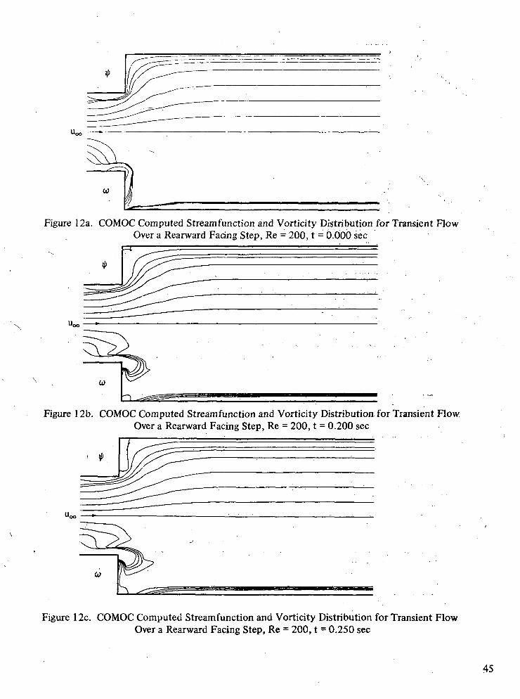
Figure 12a. COMOC Computed Stream function and Vorticity Distribution for Transient FlowOver a Rearward Facing Step, Re = 200, t = 0.000 sec

Figure 12b. COMOC Computed Stream function and Vorticity Distribution for Transient Flow,Over a Rearward Facing Step, Re = 200, t = 0.200 sec

Figure 12c. COMOC Computed Streamfunction and Vorticity Distribution for Transient FlowOver a Rearward Facing Step, Re = 200, t = 0.250 sec

45

Figure 12d. COMOC, Computed Stream function and Vorticity Distribution for Transient FlowOver a.Rearward Facing Step, Re'= 200, t = 0.500 sec

Figure 12e. COMOC Computed Streamfunction and Vorticity Distribution for .Transient FlowOver a Rearward Facing Step, Re = 200, t = 5.008 sec

Figure 12f. COMOC Computed Streamfunction and Vorticity Distribution for Transient FlowOver a Rearward Facing Step, Re = 200, t = 9.998 sec

col

Figure 12g. COMOC Computed Streamfunction and Vorticity Distribution for Transient FlowOver a Rearward Facing Step, Re = 200, t = 22.365 sec

Figure 12h. COMOC Computed Streamfunction and Vorticity Distribution for Transient FlowOver a Rearward Facing Step, Re = 200, t = 29.209 sec

46

Figure 13a. COMOC Computed Steady-State Streamfunction and Vorttcitv. for Flow over a Rearward Step, Re = 200

Figure 13b. COMOC Computed Steady-State Streamfunction and Vorticityfor Flow over a Rearward Step in Irregular Shaped Duct, Re = 200

Figure 13c. COMOC Computed Steady-State Streamfunction and Vorticityfor Flow over a Rearward Step with Internal Obstacle, Re = 200

47

was stable and the recirculation region has simply readjusted to fill the new interior domain. (Theindicated appearance of vorticity lines crossing is strictly a function of the high order curve fittingoperations in the automatic plot package.) The downstream point-of-attachment of the dividingstreamline was essentially unaffected by the changed wall shape. However, as shown in Figure 13c,the insertion of a blunt body into the solution domain drastically alters the predicted recirculationregion. The inserted obstacle was tapered downstream to preclude the shedding of vortices, henceallow attainment of the illustrated steady-state, time-independent solution. The computed vorticitysolution is markedly altered from Figure 13a, and the dividing streamline reattachment has movedto within about four step-heights downstream. The second recirculation region at the step baseis retained in both sample solutions; its apparent unstreamlined shape could be improved with addeddiscretization, and resolution could be improved if required. No independent measures are availableto assess the accuracy of either of these solutions, but the computed solutions do appear acceptableon^a physical basis. They amply illustrate the boundary shape variability that is automatically accept-able to COMOC.

Equation (75) has been evaluated for computation of static pressure distributions along thecenterplane of the duct flow problems. For two-dimensional steady flow with constant density andviscosity, Eq. (75) evaluated on the centerplane becomes

Ap = -A(- \2/,2)2 -•£- /",2dx, +-~-p Re -J pRe

In Eq. (115), the first term represents the purely dynamic pressure change due to streamline conver-gence. The second accounts for viscous dissipation, and the generic third derivative in streamfunctionhas been replaced in terms of vorticity through Eq. (40). The last term contains the viscous contribu-tion stemming from non-parallel flow. Evaluation of Eq. (115) between any two points provides thecorresponding pressure difference. For fully developed, parallel flow, only the middle term in Eq.(115) is non-vanishing and the expression is analytically exact. For general flows, evaluation of firstand second order derivatives of tabulated functions is required. In keeping with the use of linearfinite element approximation functions for computation of the flow field variables, low order dif-ference formulas appear appropriate. .

Shown in Figures 14 and 15 are the calculated static pressure distributions along the center-plane of the duct and the rearward step problems, for Re = 200, for the computed steady-state stream-function and vorticity distributions previously discussed. The total viscous contribution to Eq. (115)is separately noted in each case. For both problems, the dynamic contribution dominates the distri-bution. For the duct case, the viscous contribution near the centerplane is quite small for about 30%of the duct length. For fully developed parallel flow, the pressure decay is solely due to vorticity, andthe analytic pressure gradient for fully developed flow is also shown in Figure 14. The computed sol-ution for viscous contribution to pressure decay and total decay are observed to both be approachingthis value. Concerning accuracy, the computed streamfunction distribution predicts fully developedparallel flow to within 0.75% across the entire duct terminus. The maximum computed deviation(~ 25%) from fully developed vorticity occurs adjacent to the centerplane at the duct terminus. Theerror in computed vorticity signficantly affects the accuracy of viscous dominated pressure compu-tations which accounts for the slope dispairty at the duct terminus. In most practical flows of in-terest, viscous effects are strongest near the containing walls. For the duct flow case, the computedterminal vorticity distribution near the wall is accurate to within 2%; a corresponding improvementin accuracy of computed pressure in this region would accrue.

48

1.000O

0.975

0.950

ox

Q."a 0.925

0.900

Symbol Contributions

A Viscous

. O " Viscous and Dynamic

0.875

0.850

Fully Developed FlowPressure Decay

10 15 20Longitudinal Station - x/L

25 30

Figure 14. Centerplane Pressure Decay in Steady-State Duct Flow, Re = 200

49

Symbol Contributions

Viscous

O Viscous and Dynamic

-2.0 2.0 4.0 6.0 8.0 10.0 12.0

Longitudinal Station - x/L

Figure 15. Centerplane Pressure Distribution for Steady Flow Over a Rearward Facing Step,Re = 200

50

Solution of the Navier-Stokes equations is typically required for internal—that is, confined-flow problems as has been illustrated. A vast number of practical aerospace and aeronauticalflow field configurations correspond to external flow problems wherein a significant simplificationto the Navier-Stokes system exists as "boundary layer" theory. This equation system is parabolic forsteady flows over a wide range of Mach numbers, even for three-dimensional problems, and its solu-tion has been greatly explored, see Blottner (Reference 20). However, with the blown flap systemson todays aircraft, and/or the supersonic and hypersonic cruise speeds of the space shuttle and hyper-sonic research vehicle, there are numerous opportunities to form local regions of imbedded recircu-lation within a predominantly boundary-layer-type flow field. Classical examples for supersonicflows are shown in Figures 16 and 17 which illustrate how complex shock wave interaction can in-duce local separated flow regions. Such occurrences are of critical design importance since aerody-namic control is affected, and local heat transfer rates are significantly increased in these zones. At-tempts have been made to use the boundary layer equations for solution of shockwave-boundarylayer interaction problems (Reference 21), including the neglect of instability-producing negativeconvection terms (Reference 22). These methods have generally proven unsuccessful since thenumerical mathematics are basically incompatible with the physics of flow. The compression cornerproblem is somewhat more tractable since the approximate location of the shock, hence recirculationzone, is at least known. Extension of Navier-Stokes incompressible flow finite difference techniquesto this problem are reported (Reference 23), and a comprehensive numerical solution of the entiretransient, viscid-inviscid interaction region flow field is recently published (Reference 24). The rear-ward facing cone-step problem is particularly difficult; factors affecting the extent,of the recirculationregion are reported (Reference 25); and the results of a numerical study of the companion problemof base flow behind a wedge are published (Reference 26).

The developed finite element solution algorithm for the steady Navier-Stokes for a compress-ible fluid is potentially applicable to this problem class in conjunction with appropriate means forestablishing the required boundary conditions. For interaction problems, this typically includesknowledge of shock impingement location, as well as inflow distributions and outflow location andparameters. Inclusion of density as a computed variable is concomitant with addition of an equationof state, Eq. (7). From the definition of stagnation enthalpy, and for a perfect gas, a quadratic ex-pression for density is obtained after substitution of Eq. (37) for velocity. Only the positive root isadmissible which yields the following equation for density in terms of static pressure (ps), stagnationenthalpy (H) and streamfunction derivative.

)f '= - CP * V \-^~ I +2H (*,,) ' | (116)

The finite element solution requires establishment of density at node points of the solution domain.No complication arises from either pressure or enthalpy, since their nodal values are directly available.However, for linear approximation functipnals, the streamfunction derivative term becomes

= Mm lB211S]{* | m (117)

which is strictly element dependent. To establish a unique nodal value of density, Eq. (1 16) is evalu-ated within an element loop in COMOC, and nodal values of computed density summed into a global

51

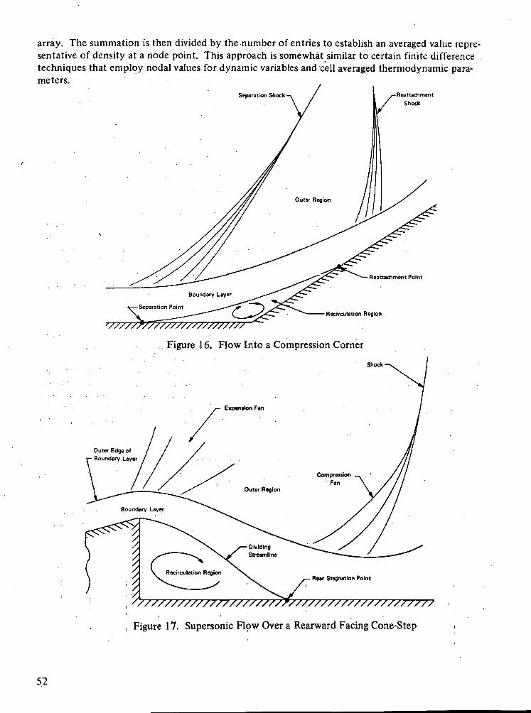
array. The summation is then divided by the number of entries to establish an averaged value repre-sentative of density at a node point. This approach is somewhat similar to certain finite differencetechniques that employ nodal values for dynamic variables and cell averaged thermodynamic para-meters.

Separation Shock Reattachment

Shock

Reattachment Point

Recirculation Region

•., Figure 16. Flow Into a Compression Corner

Shock -

Figure 17. Supersonic Flow Over a Rearward Facing Cone-Step

52

The utility of the finite element approach for analysis of compressible flows has been evaluatedin a cursory manner for two problems. Additional downstream discretization was added for the rear-ward step configuration, Figure 11, and the solution parameters scaled to simulate isoenergetic flow ofair ai M^ = 0.6, based upon a mass-averaged inlet velocity of 122 m/s (400 ft/s), and Re = 200 basedupon step height. Under these conditions, compressibility and temperature-dependent viscosity (viaSutherland's Law) should be measurable, but their combined effect should not measurably alter theessential Reynold's number invariance of the flow field. As with previous evaluations, the duct flowwas initiated impulsively and the computed recirculation zone allowed to develop during the transientsolution. Essential steady-state flow was achieved within 0.15 second; at this time, the downstreamduct terminus contained fully developed flow to within 0.125% maximum deviation, employing thevanishing normal gradient boundary condition for both streamfunction and vorticity. As expected,the contours of the computed distributions appeared very similar to those of Figure 12h. The down-stream attachment point of the dividing streamline was identically located; the attachment at the stephad moved to the comer, although a refined discretization would be required to accurately evaluateits location for this test case. As before, a second recirculation zone was predicted at the base of thestep. The null point of the primary recirculation zone occurred on the node column located sevenstep heights downstream of the step. Shown in Figure 18 are computed steady-state distributions ofthe dependent variables across the transverse dimension of the duct at this longitudinal station and atthe duct terminus. The streamfunction solution illustrates the small flow velocities occurring withinthe recirculation zone; a null point in vorticity is correspondingly indicated. Freestream densityoccurs within this region, and the "pinch" effect of the recirculation zone correspondingly increasedmain flow density by up to 5%. The computed viscosity distributions similarly show largest variationsoutside the recirculation region.

The finite element solution procedure may be useful for studies of imbedded recirculationzones within boundary layer flows, provided boundary conditions are available and shock locationsknown. The supersonic compression corner falls into this category, and a computational solutionmight involve establishing the vorticity-streamfunction equivalent of supersonic boundary layer flowas an initial condition, and then bending the plate surface, and skewing the discretization downstreamof the hinge, to the required angle. Illustrations of sample discretizations for such a procedure areshown in Figure 19, for the geometry studied by Carter (Reference 24). The existence of the shockin Figure 19b could be computationally simulated by the (jump) parallel-velocity boundary conditionfor streamfunction, Eq. (101). As an introductory step to analysis of this problem, the discretiza-tion of Figure 19a was employed by COMOC to solve for the vorticity-streamfunction equivalent ofsupersonic laminar boundary layer flow of air for Moo = 3.0, and Re = 7750, based upon distancefrom the plate leading edge to the midpoint of the solution domain. The inflow boundary conditionfor streamfunction, and slope of the top of the solution domain, were established using Eq. (99) anda similarity solution for boundary layer flow. The vorticity distribution at inflow was establishedfrom its definition, Eq. (39), vanished along the top, and was evaluated on the no-slip plate surfaceusing Eq. (103). The vanishing normal gradient, although locally incorrect for boundary layer flows,was employed downstream for both variables. Shown in Figure 20a is the computed essential steady-state vorticity distribution ({ n}' < 0.001) for the domain of Figure 19a. A high plateau of vorticityexists near the plate surface which drops off rapidly as freestream is approached. Figure 20b com-pares computed streamfunction and density distributions at x/L = 1.0 to corresponding valuesobtained from the similarity solution. Agreement is good except for density near the freestream,where use of Eq. (116) rounded the distribution. This may result from a poor local speed approxima-tion, using Eq. (117), for regions with large gradients in streamfunction; a finer discretization should

53

improve results. The accuracy of computed stream function at the downstream terminus wasnoticeably poorer, as a direct consequence of the applied gradient boundary condition. Judgingfrom these results, it appears adequate to extend the solution domain a distance of x/L = 1 down-stream of the region of interest for this problem. Furthermore, use of Eq. (116) appears valid forcompressible flows when combined with attention to discretization.

CONCLUDING REMARKS

A finite element algorithm for solution of problems in the two-dimensional Navier-Stokesequations has been established. Numerical evaluation within the COMOC computer program systemhas produced a favorable assessment of solution accuracy and convergence. The versatility of the codehas been illustrated for several problem variations. It appears that the finite element approach of com-putational fluid mechanics exhibits much of the required generality and flexibility to serve as aneffective design and communication tool between the engineer and scientist and the present and nextgeneration of digital computer systems.

54

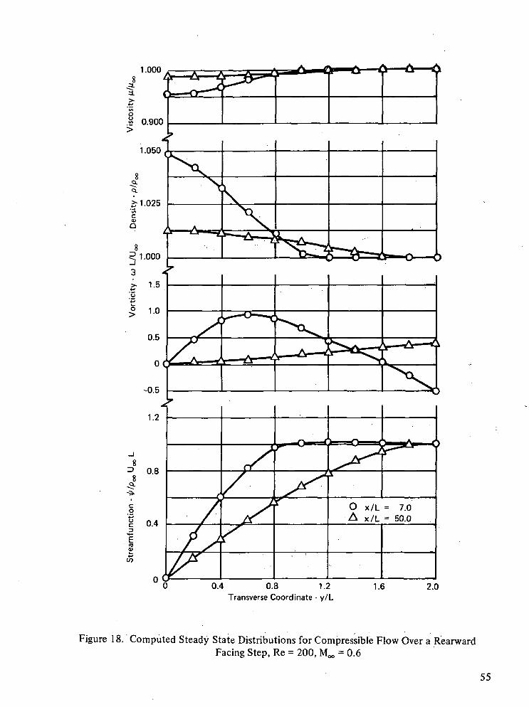
1.000

O x/L = 7.0A x/L = 50.0

0.4 0.8 1.2Transverse Coordinate - y/L

Figure 18. Computed Steady State Distributions for Compressible Flow Over a RearwardFacing Step, Re = 200, M^, = 0.6

55

0.12 +

0.00

0.6 0:7 0.8 0.9 1.0 1.1Longitudinal Coordinate - x/L

(a) Flat Plate, M = 3.0

1.2 1.3 1.4 1.5

0.404-

0.00

0.5 0.6 0.8 0.9 1.0 1.1

Longitudinal Coordinate - x/L(b) Compression Corner, Mx - 3.0

1.2 1.3 1.4 1.5

Figure 19. Finite Element Discretizations for Supersonic Boundary Flows

56

80

CO

C>

CM

O

pO

8O

q

ii

cO

>

0)

OOO

cto

inoo"

c0)Q•aCO

O"4-1Oc3

*4-

CO

CO

3O

03

CO

CX3

C/3

05

O

CO

O

iqci

°d/d •

o'o

CO

o

CO

3agoUo(N

60

57

APPENDIX ACARTESIAN TENSORS IN EUCLIDEAN SPACE

In the rectangular Cartesian coordinate description of Euclidean space, Xj = { x, y, z } , simplesubscript tensor notation and the summation convention are sufficient to describe the calculus oftensor fields. In general curvilinear coordinates, the completely general tensor formalism involvingco- and contra-variant scalar components and basis vectors is required, see Reference (27). Whendealing with orthogonal curvilinear (i.e., Cartesian) coordinate systems, simple tensor notation isinadequate and the full power of the general tensor is not needed since no distinction exists betweenthe two variant forms.

The appropriate mathematical tool for tensor field calculus operations in Cartesian coordin-ates is Cartesian tensor analysis in Euclidean space, Reference (28). The,basic concept of geometryis the infinitesimal displacement ds. Denoting yj as the rectangular Cartesian components of anarbitrary position vector7, and xj as the scalar components in any other Cartesian basis, an arbitraryvector can be written as

7= y- f i j = XjTj (A-l)

where a^ are the (constant) unit vectors (i, j, k) and e^ are any other orthogonal basis vector set. Theinfinitesimal displacement (squared) becomes

ds2 = dT-df = dyj£|-dyja: = dyj dy^ (A-2)

since contraction of Unit vectors in the rectangular basis yields the Kronecker delta.. A similar formis obtained for any orthogonal basis, with the exception that, since the basis vectors are not in gen-eral unit vectors, their contraction will yield scalar coefficients modifying the Kronecker delta. De-noting these as h: , the general form is

ds2 = (A-3)

where the subscript bar denotes the index is not included in the summation convention. The h: arecalled metric coefficients and are functions of the particular coordinate system-. For example, incylindrical coordinates with Xj = jz, r, 6\

In spherical coordinates with Xj = jr, 0, 0} , with <j> the polar angle with domain 0 <x2 <TT,

h^ = |l,r, rsin0} ^A_5^

It is desirable to establish an orthonormal basis for the general Cartesian description. Considering ageneral vector field "v (as described by the form of equation A-l), with scalar components Vj andbasis <Tj, multiply and divide by hj to obtain

7 = h: V: — = U-^-11 hi Vl (A-6)

59

In equation A-6, U: (= hj Vj) are called the physical components of the vector v", and 6j are unit vectorsof the orthonormal basis.

The fundamental calculus operation requiring identification is differentiation. Referring toequation A-6, the derivative of v" with respect to the Xj variables is, using the chain rule

9 A,

(A'7)

The last term in equation A-7 describes the change in the unit vector e-. with respect to x:. Sincethis is also a vector, it can be described by scalar components projected on the £j basis. The coeffi-cients of proportionality for this description are the physical components of the Christoffel symbolsof general tensors, contracted over index pairs. They have been termed "wryness" coefficients, Ref-erence (29); signifying them by wy^ and expressing fin the £j basis, equation A-7 becomes

37 :s»i;A-(^j.+ ^k.V*i -<*•«>dxjIn equation A-8, the spatial (vector) derivative of a vector is signified by the semicolon. The partialderivative of a scalar (component) is denoted by the comma. Since equation A-8 is a vector identitythe scalar components are identical. Hence

u i ; j ~ ui,j + wijkuk (A-9)

defines the vector derivative of the scalar components of a vector (first order tensor) in an arbitraryorthonormal basis. Equation A-9 can be readily generalized to the vector derivative of the scalarcomponents of an n*n order tensor, see Reference (28). . .

The properties of the wryness coefficients are readily determined. They are not scalar com-ponents of a third, order tensor -since they do not obey the tensor transformation law. All componentsvanish for the indices distinct. The coefficients are skew-symmetric in all index pairs. Hence, theonly nonvanishing terms are of the form

"kjk =-"jkk (A-10)

In particular, the singular nonvanishing coefficient in cylindrical coordinates is

"233 = 7- (A-ll)

In spherical coordinates, obtain .

"122 = W i 3 3 =— (A- 12)

60

J233

From equation A-9, the vector derivative of a scalar is simply the partial derivative withrespect to Xj, commonly referred to as the gradient. From equations A-l, A-3, and A-6, obtain

Equation A-14 defines the partial derivative, signified by the comma. Equating scalar coefficients,obtain by components

The operation of curl is the contraction of equation A-9 with the general alternating tensor ejjk,which is skew symmetric in all index pairs and has positive scalar components for (i, j, k) in thecyclic order (1, 2, 3). Hence,

curl ?.% = eijk uk .j (A-16)

The general alternating tensor is related to the Cartesian alternating tensor qjk, with unit magnitudescalar components, by the determinant of the space metric, which for Cartesian tensors is simply theproduct

J^ ht h2 h3 (A-l 7)

Equating scalar coefficients in equation A-16, and using equation A-17, obtain for the i* componentthe curl of the vector ~v

cur lv-^ = y e i j k u k ; j (A-l 8)

Equations A-3, A-9, A-10, A-l 5, and A-18 are sufficient to facilitate the calculus of Cartesiantensors in Euclidean space. Integral theorems, developed for rectangular Cartesian tensor fields,transform directly to general Cartesian tensor fields. Of particular interest, the divergence theorembecomes, for an arbitrary order Cartesian tensor field Tjjk. . . ,

(A-l 9)/R CTijk - • • ) ; « dr = R (Tijk . . . ) - ,<, da

where v% is the unit outward pointing normal vector to the closure 3R of the domain R. Similarly,for Stokes' theorem obtain

[ (curl Tiik . . . ) . i/p da = <£ T (Tijk . . . ) . te ds (A-20)J9R J J dL

where 9L is the bounding curve of the closure 3R and tj is the unit vector everywhere tangent to 9L.

61

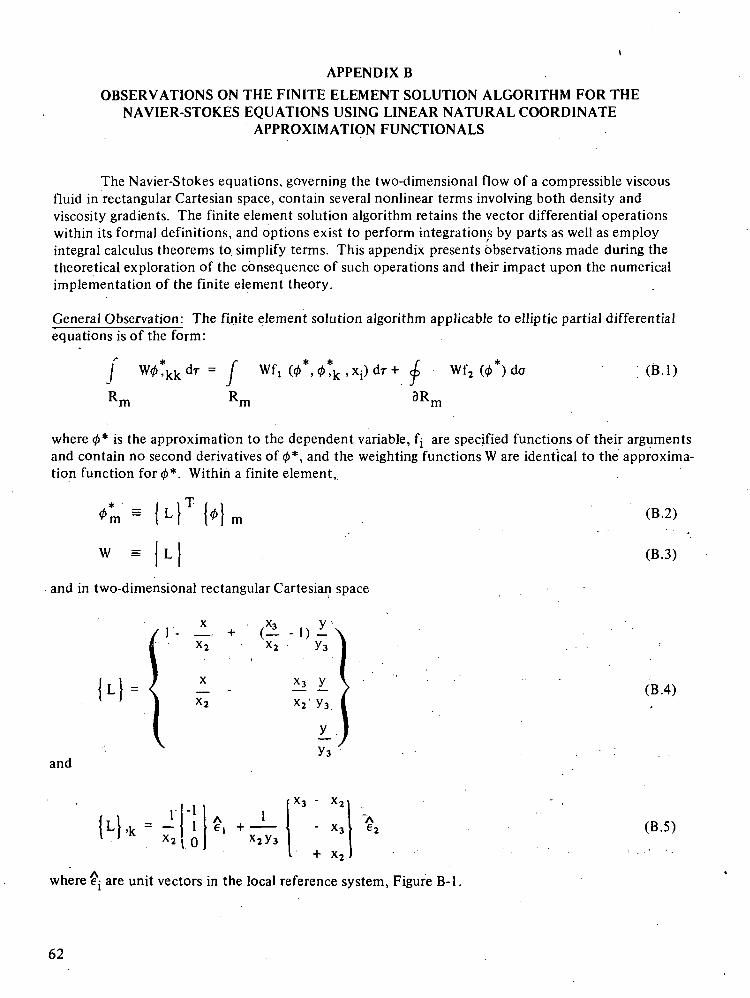
APPENDIX B

OBSERVATIONS ON THE FINITE ELEMENT SOLUTION ALGORITHM FOR THENAVIER-STOKES EQUATIONS USING LINEAR NATURAL COORDINATE

APPROXIMATION FUNCTIONALS

The Navier-Stokes equations, governing the two-dimensional flow of a compressible viscousfluid in rectangular Cartesian space, contain several nonlinear terms involving both density andviscosity gradients. The finite element solution algorithm retains the vector differential operationswithin its formal definitions, and options exist to perform integrations by parts as well as employintegral calculus theorems to simplify terms. This appendix presents observations made during thetheoretical exploration of the consequence of such operations and their impact upon the numericalimplementation of the finite element theory.

General Observation: The finite element solution algorithm applicable to elliptic partial differentialequations is of the form:

W0?kkdr = Wf, (0*,0?k ,x i)dr+ Wf2 da (B.I)

Rm Rm m

where 0* is the approximation to the dependent variable, fj are specified functions of their argumentsand contain no second derivatives of 0*, and the weighting functions W are identical to the approxima-tion function for 0*. Within a finite element,

= j Lm

W = L

and in two-dimensional rectangular Cartesian space

(B.2)

(B.3)

(M-

x x, y_ + (-i -1)1x2 x2 y3

x 2 ' y 3 .(B.4)

andV3

X3 - X2

X2

(B.5)

where €j are unit vectors in the local reference system, Figure B-l.

62

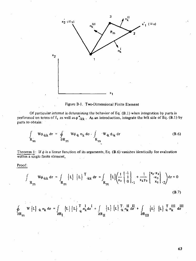
*2 « =

. Figure B-l. Two-Dimensional Finite Element

Of particular interest is determining the behavior of Eq. (B. 1) when integration by parts isperformed on terms of ft as well as0 tfck • As an introduction, integrate the left side of Eq. (B.I) byparts to obtain:

/ W0,Rm

kk dr =9Rm

, k n k d o - J W,k0,kdr

R,

(B.6)

m

Theorem 1: If 0 is a linear function of its arguments, Eq. (B.6) vanishes identically for evaluationwithin a single finite element,

Proof:

Rm Rm

,kkdr =/Rm

-1

0-x3 )dr = 0x^ I '2/

(B.7)

3Rm

W ILJ >lr nk do = f J L J l L J nuda1 + f \L\I I "• K j t I I J >k R ./ < 'dRi 3R,in 3Rm

T III III,1, ni, da

63

2y3|X3'X2, "X3 ,X2|

2x2y3

1(x2y3)2

sym

[B211S]m(0) m

(X3-X2)2 , -X3(X3-X2) , X2(X3-X2J

2x2

(B.8)

Rm Rm

• /RR

[L),k

-1, 1,0 . + m

(B.9)

Combining Eq. (B.8) and Eq. (B.9), the identity in zero is accomplished, Q.E.D.

Theorem 2: If 0 is a linear function of its arguments, the surface integral contributions resultingfrom integration by parts, Eq. (B.I), can be made to cancel in pairs upon assembly, by Booleanalgebra, of the global solution algorithm.

Proof: Along the line common to the finite elements defined by domains RI and RJJ, Figure B-2,specify the local value of the normal gradient of the function 0 as an algebraic average. The coin-cident portion of the closed surface integral for each domain becomes

64

= x, x

X2

(=Y)

Figure B-2. Adjacent Finite Elements

J W0,k nk da = f

3Rr

0,kn + - 0 , n dx (B.10)

f rJ W0,knkda =J

1 I II 1 II IIdx

o

I IISince nk = -nk , and using Eq. (B.2) - (B.5), along the common line,

/ < >" -* • (-J™ 4 10 V

(B. l l )

(B.12)

9R)dx =-r

II

( x 3 - x 2 > - x 3 , x 2 } j 0 } 1 - - — (x3-x2 ,-x3 ,x2 [ J0)n j

(B.13)

65

Upon Boolean assembly of Eq. (B. 12) and (B. 13), the first of each equation" is loaded into the globalvector on 10} at the location 0j. Hence, cancellation by pairs is achieved for the surface integral.contributions stemming from Eq. (B.6), Q.E.D..

Theorem 3: If 0 is a linear function of its arguments, and Eq. (B.I) involves a scalar nonlinearitythat is not differentiated, the surface integral contribution stemming from integration by parts canbe made to vanish in pairs upon Boolean assembly of the global solution vector.

Proof: The compatibility equation for the two-dimensional Navier-Stokes equation can be integratedb y . parts, a s . . . . . . . . .

R 3R

(B.14)

R

Using the averaging concept developed in the previous proof, obtain from Eq. (B.14) on an elementbasis:

= f- (L) nkdo (B.15)m

Along the line connecting nodes 1 and 2, Figure B-2, Eq. (B.15) becomes, using Eq. (B.4) and (B.5)within elements Rj and RJJ,

f ( ) da = —! 1 0"

2 0_sym 0

(B.I 6)

/ _sym

1 ° r 1 i /I *I • 1 , *II2 11 l7ln(+2**.-2**

(B.I 7)

The only elements of the finite element matrix I—1 involved in non-zero products in Eq. (B.I6)[P 'm

and (B.I7) are for node locations on the common line. Hence, upon Boolean assembly, the con-tributions from surface integrals involving a scalar nondifferentiated nonlinearity cancel by pairs,Q.E.D.

Observation: The convection term, involving the curl of the streamfunction (vector potentialfunction), appears in the differential equation and finite element description for each dependentvariable except streamfunction. An integration by_ parts is possible.

Theorem 4: Within the convection operator, and for 0 a linear function of its arguments, noarbitrariness exists for evaluation of the generated surface integral.

66

Proof: The typical convection term is, upon integration by parts,

W ke3k i

Rm 3Rm Rm

For the surface integral, using Eq. (B.2) - (B.5), obtain

da = f (L| (L}T {n}m6 3 k i{LlT , in kdo U m (B.19)

Note that the gradient operator on JL| is orthogonal to the local normal via the alternator. Fromthe natural coordinate function description, Eq. (B.4), such derivatives involve end point nodal valuesonly. Hence, for integration over the three sides of the finite element, Figure B-l, obtain

m

f2 1 0"2 0

L 0.

0-1

1

0 0 0]2 1 + M [20 MV io | [oo j ) | , } m

(B.20)

Evaluating the remaining term on the right side, and subtracting it from Eq. (B.20) produces theidentity. Hence, there is no arbitrariness in evaluating the terms stemming from this integration byparts, Q.E.D.

Straightforward evaluation of Eq. .(B.18) for linear functional yields

/ We3ki(c^,i),kdr = f { L } 6 3 k i { ^ } m ( L } , i 6 3 k i ( L } Tk d r In} (B.21)

Rm Rm

The alternator contraction produces the skew-symmetric matrix.

T>ke3ki

Equation (B.21) takes the form:

j[' -!

[I

(B.22)

-1 1

0 -1

1 OJ(B.23)

Observation: The finite element solution algorithm produces several nonlinear matrix forms thatare eligible for integration by parts. For example, in the differential equation for vorticity, anadditional convection term results for nonuniform density flows of the form:

67

Rm

This term vanishes identically, for linear functional approximations, unless an integration by partsis performed. Hence,

r L l i i r l 1/ ( ) dr = <p Weoi,: (—) , k —(i / / ,p ) 2 n{ da - / W,k e^i (~)>kT W.p) dr7 j JKI - K 2 * i J. K •>*•! p K 2R H D UO i\_^_ ^x**^m m m

(B.24)

Equation (B.24) vanishes identically for <//,£ evaluated solely within Rm. However,

Theorem 5: Using linear functional representations for all dependent variables, the surface integralcontribution to Eq. (B.24) can be made to cancel by pairs, upon Boolean assembly of the globalsolution algorithm, by averaging the available derivative operations over closure segments of therespective finite elements.

Proof: Referring to Figure B--2, along the common closure segment connecting nodes 1 and 2, thesurface integral contributions within Rj and RTT can be written as

f \ . I I — 1 I T - I I I I I 5V I I I I ' V I T I I I - - S 1 C I I I 5 I T I I "1 — • - \D.£J)

O

(B.26)2 J

3Rn o

Since the inner product on i//,g is commutative, and since the alternator e^[ removes arbitrarinessin the evaluation of JLj ,k , and since nj are antiparallel, then upon Boolean assembly of Eq. (B.25)

and (B.26) into the global vector, cancellation by pairs is achieved, Q:E.D.

Completion of the matrix form of Eq. (B.24) is straightforward.

) dr = - J

The inner contraction upon i//,g involves the matrix [B21 IS] , Eq. (B.8), while the alternator con-traction produces the negative of Eq. (B.22). Hence, the final form becomes:

T{ ( )dr = + 1 I<M [B211S] ji//l 1 0 -1 Ul (B.27)

JR 4 . - 1 1 Oj ^ Jm

68

APPENDIX C

SYSTEM INVARIANCE UNDER COORDINATE TRANSFORMATION

Use of a locally defined coordinate system for matrix moment evaluation is desirable from theaccuracy standpoint and mandatory for evaluation of the nonlinear terms in the Navier-Stokes equa-tions, The classical Method of Weighted Residuals (MWR) solution to a differential equation, N(q) =0, involves approximation of the dependent variable by a function, q*, and rendering the error ortho-gonal to the solution by formation of the residuals

f W:N(q*)dT = 0 (C.I)JR

The finite element algorithm transforms formation to a finite element Rm, and there are as many equa-tions (C. 1) as unknown expansion coefficients in qm on a local basis. The theoretical complicationstemming from gradient boundary conditions can be neglected for this development.

Use of natural coordinate functions in a local Cartesian basis is preferred; hence, it is necessaryto transform Eq. (C. 1) from the global basis of its derivation. Assuming use of truncated power series,and to within an arbitrary coordinate translation, see Figure C. 1, the global reference approximationfunction can be expressed as

qm(Xi) = [x-X]T[r]m{Q}m (C.2)

In Eq. (C.2), the elements of the coefficient matrix [Y ] m involve only node point coordinates1 of Rm

and are readily evaluated (reference 12). It is required to establish Eq. (C.2) in the xj basis, related toXj by the tensor transformation law

xj = fly (Xj-Xj) (C.3)

or equivalently, in matrix notation

j x ' } ' = [0],-{x-X| - ' (C.4)

In the primed coordinate system, Eq. (C.2) takes the form

q m (xj ) = |x'}T[r ']m |Q}m . (C.5)

Combining Eqs. (C.4) and (C.2), and comparing to Eq. (C.5) provides the definition of [T1] m as

ir']m = [0]'1 ir]m (C.6)

Identifying the weighting functions for the Galerkin criterion within MWR as

wm = [r]T jx-x} (C.7)J m

69

X 2

X2

X1

Figure C-l. Coordinate Systems for the Finite Element Solution Algorithm

70

and substituting Eqs. (C.4) - (C.I) into Eq. (C.I), the finite element residual expression for determina-tion of the matrix elements of JQ) becomes of the form

K= 0 (C.8)

m

It remains to cast the integration kernel dr into the primed coordinate system to allow evalua-tion of equation (C.8) entirely in a local basis. From tensor field theory (reference 27), integrationkernels in respective spaces spanned by Cartesian coordinate systems are linearly related by the determ-inant of the Jacobian of the transformation from a rectangular Cartesian basis, y^, as

dr' - T- drIII

where

[J] =

(C.9)

(CIO)

The determinant of the Jacobian for transformation to another rectangular Cartesian basis is unity.However, transformation to either cylindrical or spherical coordinates introduces nonvanishing coef-ficients. Hence, f o r t he three subject transformations obtain, respectively • . . . . !

di-' = dr

(C.I 1)= x,sinx2dT

For cylindrical coordinates and' axisymmetry,

x2 = x2O + x', sin a + x2 cos a (C.I 2)

where x2 ^ MS the radial coordinate of node 1 for Rm, Figure C.I . The equivalent expression fornatural coordinate functions defined by

qm

becomes

(C.I 3)

(C.14)

71

REFERENCES

1. Finlayson, B. A., and Scriven, L. E., "The Method of Weighted Residuals - A Review," App.Mech. Rev., \9, No. 9, 1966, 735-748.

2. Finlayson, B. A., and Scriven, L. E., "On the Search for Variational Principles," Int. J. HeatMass Trans., K), No. 6, 1967, 799-821.

3. Gurtin, M. E., "Variational Principles for Linear Initial-Value Problems," Q. App. Math, 22,1964,252.

4. Wilson, E. L., and Nickell, R. E., "Application of the Finite Element Method to HeatConduction Analysis," Nuc. Engr.,Design, 4, 1966, 276-286.

5. Baker, A. J., "A Numerical Solution Technique for Problems in Heat Transfer Employing theCalculus of Variations," Bell Aerospace Technical Note TCTN-1003, 1968.

6. Baker, A. J., "Numerical Solution to the Dynamics of Viscous Fluid Flow by a Finite ElementAlgorithm; A First Step Towards Computational Continuum Mechanics," ProceedingsInternational Association for Shell Structures Pacific Symposium on.HydromechanicallyLoaded Shells, 1971.

7. Baker, A. J., "Finite Element Computational Theory for Three-Dimensional Boundary LayerFlow," AIAA Paper 72-108, 1972.

8. Baker, A. J., "Finite Element Solution Algorithm for Viscous Incompressible FluidDynamics," Int. J. Num. Mtd. Engf., 6. No. 1, 1973,89-101.

9. Baker, A. J., and Zelazny, S. W., "A Theoretical Study of Mixing Downstream of TransverseInjection Into a Supersonic Boundary Layer," NASA CR-112254, 1972.

10. Hains, F. D and Baker, A. J., "Binary Diffusion of a Jet Imbedded in a Boundary Layer,"AIAA J., 10, No. 7, 1972, 938-940.

11. Baker, A. J., and Manhardt, P. D., "Finite Element Solution for Energy Conservation Using aHighly Stable Explicit Integration Algorithm," NASA CR-130149, 1972.

12. Zienkiewicz, O. C., The Finite Element Method in Engineering Science, McGraw Hill,London, 1971.

13. Schlichting, H., Boundary Layer Theory, McGraw Hill, New York, 1960.

14. Gosman, A. D., Pun, W. M., Runchal, A. K., Spalding, D. B., and Wolfshtein, M., Heat andMass Transfer in Recirculating Flows, Academic, London, 1969.

15. Carslaw, H. S., and Jaeger, J. C.. Conduction of Heat in Solids, 1st Ed., Oxford, London,1948,275.

72

16. Gear, C. W., "Simultaneous Numerical Solution of Differential - Algebraic Equations," IEEETrans., CT-18, 1971, 89-95.

17. Mueller, T. J. and O'Leary, R. A., "Physical and Numerical Experiments in LaminarIncompressible Separating and Reattaching Flows," AIAA Paper 70-763, 1970.

18. Dorodnitsyn, A. A., "Review of Methods for Solving the Navier-Stokes Equations,"Proceedings Third Int. Conf. on Num. Mtd. in Fluid Mechanics, 1973, 1-11.

19. Macagno, E. O. and Hung, T. K., "Computational and Experimental Study of a CaptiveAnnular Eddy," J. Flu. Mech. 28, 1, 1967, 43-64.

20. Blottner, F. G., "Finite Difference Methods of Solution of the Boundary Layer Equations,"AIAA J., 8, No. 2, 1970, 192-205.

21. Murphy, J. D., "A Critical Evaluation of Analytic Methods for Predicting Laminar BoundaryLayer Shock-Wave Interactions," NASA SP-228, 1969.

22. Reyhner, T. and Flugge-Lotz, I., "The Interaction of a Shock Wave with a Laminar BoundaryLayer," Int. J. Nonlinear Mech., 3, 1968, 173.

23. Roache, P. J. and Mueller, T. J., "Numerical Solutions of Laminar Separated Flows," AIAA J.,8, No. 3, 1970,530-538.

24. Carter, J. A., "Numerical Solutions of the Navier-Stokes Equations for The SupersonicLaminar Flow Over a Two-Dimensional Compression Corner," NASA TR R-385, 1972.

25. Ball, K.O.W., "A Summary of Factors Influencing the Extent of Separation of a LaminarBoundary Layer Due to a Compression Corner at Moderately Hypersonic Speeds,"ARL 71-0065, 1971.

26. Carpenter, P. W., "A Numerical Investigation into the Effects of Compressibility and TotalEnthalpy Difference on the Development of a Laminar Free Shear Layer," J. Flu. Mech.,50,4,1971,785-799. ,

27. Sedov, L. I., Foundations of the Nonlinear Mechanics ofContinua, Chap. 1, Pergamon,London,1966.

28. Jaunzemis, W., Continuum Mechanics, Chap. 1, MacMillan, New York 1967.

29. Ericksen, J.L. and Truesdell, C., "Exact Theory of Stress and Strain in Rods and Shells,'Arch, for Rat. Mech. and Anal.,_L 1958, 295-323.

U*. GOVERNMENT PRINTING OPFICEl 1*74-7 JJ-7H/* 7 REGION NO. 3-11

NATIONAL AERONAUTICS AND SPACE ADMINISTRATION

WASHINGTON. D.C. 2OS46

OFFICIAL BUSINESS

PENALTY FOR PRIVATE USE S3OO SPECIAL FOURTH-CLASS RATEBOOK

POSTAGE AND FEES PAIDNATIONAL AERONAUTICS AND

SPACE ADMINISTRATION451

POSTMASTER : If Undellverable (Section 158Postal Manual) Do Not Return

"The aeronautical and space activities of the United States shall beconducted so as to contribute . . . to the expansion of human knowl-edge of phenomena in the atmosphere and space. The Administrationshall provide for the widest practicable and appropriate disseminationof information concerning its activities and the results thereof."

—NATIONAL AERONAUTICS AND SPACE ACT OF 1958

NASA SCIENTIFIC AND TECHNICAL PUBLICATIONSTECHNICAL REPORTS: Scientific andtechnical information considered important,complete, and a lasting contribution to existingknowledge.

TECHNICAL NOTES: Information less broadin scope but nevertheless of importance as acontribution to existing knowledge.

TECHNICAL MEMORANDUMS:Information receiving limited distributionbecause of preliminary data, security classifica-tion, or other reasons. Also includes conferenceproceedings with either limited or unlimiteddistribution.

CONTRACTOR REPORTS: Scientific andtechnical information generated under a NASAcontract or grant and considered an importantcontribution to existing knowledge.

TECHNICAL TRANSLATIONS: Informationpublished in a foreign language consideredto merit NASA distribution in English.

SPECIAL PUBLICATIONS: Informationderived from or of value to NASA activities.Publications include final reports of majorprojects, monographs, data compilations,handbooks, sourcebooks, and specialbibliographies.

TECHNOLOGY UTILIZATIONPUBLICATIONS: Information on technologyused by NASA that may be of particularinterest in commercial and other non-aerospaceapplications. Publications include Tech Briefs,Technology Utilization Reports andTechnology Surveys.

Details on the availability of these publications may be obtained from:

SCIENTIFIC AND TECHNICAL INFORMATION OFFICE

NATIONAL A E R O N A U T I C S A N D S P A C E A D M I N I S T R A T I O N

Washington, D.C. 20546