A flexible mathematical model for matching of 3D surfaces andattributes

Devrim Akca, Armin GruenChair of Photogrammetry and Remote Sensing, Swiss Federal Institute of Technology (ETH) Zurich

ETH Hoenggerberg, CH-8093 Zurich, Switzerland, E-mail: <akca><agruen>@geod.baug.ethz.ch

ABSTRACT

An algorithm for the least squares matching of overlapping 3D surfaces is presented. It estimates the transformationparameters between two or more fully 3D surfaces, using the Generalized Gauss-Markoff model, minimizing the sum ofsquares of the Euclidean distances between the surfaces. This formulation gives the opportunity of matching arbitrarilyoriented 3D surfaces simultaneously, without using explicit tie points. Besides the mathematical model and executionaspects we give further extension of the basic model. The first extension is the simultaneous matching of sub-surfacepatches, which are selected in cooperative surface areas. It provides a computationally effective solution, since it matchesonly relevant multi-subpatches rather than the whole overlapping areas. The second extension is the matching of surfacegeometry and its attribute information, e.g. reflectance, color, temperature, etc., under a combined estimation model. Wegive practical examples for the demonstration of the basic method and the extensions.

Keywords: Least squares 3D surface matching, point clouds, registration, laser scanning, intensity matching

1. INTRODUCTION

For 3D object modeling data acquisition must be performed from different standpoints. The derived local point cloudsmust be transformed into a common system. This procedure is usually referred to as registration. In the past, severalefforts have been made concerning the registration of 3D point clouds. One of the most popular methods is the IterativeClosest Point (ICP) algorithm developed by Besl and McKay1, Chen and Medioni2, and Zhang3. The ICP is based on thesearch of pairs of nearest points in the two sets, and estimating the rigid transformation, which aligns them. Then, therigid transformation is applied to the points of one set, and the procedure is iterated until convergence. The ICP assumesthat one point set is a subset of the other. When this assumption is not valid, false matches are created, that negativelyinfluence the convergence of the ICP to the correct solution4.Several variations and improvements of the ICP method have been made5,6. From a computational expense point of viewit is highly time consuming due to the exhaustive search for the nearest point7. In Besl and McKay1, and Zhang’s3 worksthe ICP requires every point in one surface to have a corresponding point on the other surface. An alternative approach tothis search schema was proposed by Chen and Medioni2. They used the distance between the surfaces in the directionnormal to the first surface as a registration evaluation function instead of point–to–nearest point distance. This point-to-tangent plane distance idea was originally proposed by Potmesil8. In Dorai et al.9 the method of Chen and Medioni wasextended to an optimal weighted least-squares framework. Zhang3 proposed a thresholding technique using robuststatistics to limit the maximum distance between points. Masuda and Yokoya5 used the ICP with random sampling andleast median square error measurement that is robust to a partially overlapping scene. Okatani and Deguchi10 proposedthe best transformation of two range images to align each other by taking into account the measurement error properties,which are mainly dependent on both the viewing direction and the distance to the object surface.The ICP algorithm always converges monotonically to a local minimum with respect to the mean-square distanceobjective function1. It does not use the local surface gradients in order to direct the solution to a minimum. Originally, itwas not designed to register multi-scale range data. Several reviews and comparison studies about the ICP variantmethods are available in the literature11-13. In Neugebauer14 and Szeliski and Lavallee15 two gradient descent type ofalgorithms were given. They adopt the Levenberg-Marquardt method for the estimation.Since 3D point clouds derived by any method or device represent the object surface, the problem should be defined as asurface matching problem. In Photogrammetry, the problem statement of surface patch matching and its solution methodwas first addressed by Gruen16 as a straight extension of Least Squares Matching (LSM).

Videometrics VIII, edited by J.-Angelo Beraldin, Sabry F. El-Hakim, Armin Gruen, James S. Walton,Proc. of SPIE-IS&T Electronic Imaging, SPIE Vol. 5665 © 2005 SPIE and IS&T · 0277-786X/05/$15

184

There have been some studies on the absolute orientation of stereo models using Digital Elevation Models (DEM) ascontrol information. This work is known as DEM matching. The absolute orientation of the models using Digital TerrainModels (DTM) as control information was first proposed by Ebner and Mueller17, and Ebner and Strunz18. Afterwards,the functional model of DEM matching has been formulated by Rosenholm and Torlegard19. This method basicallyestimates the 3D similarity transformation parameters between two DEM patches, minimizing the sum of squares ofdifferences along the Z-axes. Several applications of DEM matching have been reported20-23.Maas24 successfully applied a similar method to register airborne laser scanner strips, among which vertical andhorizontal discrepancies generally show up due to GPS/INS accuracy problems. Another similar method has beenpresented for registering surfaces acquired using different methods, in particular, laser altimetry and photogrammetry25.Furthermore, techniques for 2.5D DEM surface matching have been developed, which correspond mathematically toLeast Squares Image Matching. The DEM matching concept can only be applied to 2.5D surfaces, whose analyticfunction is described in the explicit form as a single valued function, i.e. z=f (x, y). 2.5D surfaces are of limited value incase of generally formed objects.When the surface curvature is either homogeneous or isotropic, as it is the case with all second order surfaces, e.g. planeor sphere, the geometry based registration techniques will probably fail. In some studies surface geometry and intensity(or color) information has been combined in order to solve this problem26-29.The LSM16 concept has been applied to many different types of measurement and feature extraction problems due to itshigh level of flexibility and its powerful mathematical model: Adaptive Least Squares Image Matching, GeometricallyConstrained Multiphoto Matching, Image Edge Matching, Multiple Patch Matching with 2D images, Multiple Cuboid(voxel) Matching with 3D images, Globally Enforced Least Squares Template Matching, Least Squares B-spline Snakes.For a detailed survey the authors refer to Gruen30. If 3D point clouds derived by any device or method represent an objectsurface, the problem should be defined as a surface matching problem instead of the point cloud matching. In particular,we treat it as least squares matching of overlapping 3D surfaces, which are digitized/sampled point by point using a laserscanner device, the photogrammetric method or other surface measurement techniques. This definition allows us to finda more general solution for the problem as well as to establish a flexible mathematical model in the context of LSM.Our mathematical model is another generalization of the LSM16, as for the case of multiple cuboid matching in 3D voxelspace31,32.Our proposed method, Least Squares 3D Surface Matching (LS3D), estimates the 3D transformation parameters betweentwo or more fully 3D surface patches, minimizing the sum of squares of the Euclidean distances between the surfaces.This formulation gives the opportunity of matching arbitrarily oriented 3D surface patches. An observation equation iswritten for each surface element on the template surface patch, i.e. for each sampled point. The geometric relationshipbetween the conjugate surface patches is defined as a 7-parameter 3D similarity transformation. This parameter spacecan be extended or reduced, as the situation demands it. The constant term of the adjustment is given by the observationvector whose elements are Euclidean distances between the template and search surface elements. Since the functionalmodel is non-linear, the solution is iterative. The unknown transformation parameters are treated as stochastic quantitiesusing proper a priori weights. This extension of the mathematical model gives control over the estimation parameters.The details of the mathematical modeling of the proposed method, precision and reliability issues, convergence behavior,and the computational aspects are explained in the following section. The further extensions to the basic model are givenin the third section. Two practical examples for the demonstration of the basic method and the extensions are presentedin the fourth section.

2. LEAST SQUARES 3D SURFACE MATCHING (LS3D)

2.1. The basic estimation modelAssume that two different partial surfaces of the same object are digitized/sampled point by point, at different times(temporally) or from different viewpoints (spatially). Although the conventional sampling pattern is point based, anyother type of sampling pattern is also accepted. ),,( zyxf and ),,( zyxg are conjugate regions of the object in the leftand right surfaces respectively. The problem statement is finding the correspondent part of the template surface patch

),,( zyxf on the search surface ),,( zyxg .

),,(),,( zyxgzyxf = (1)

SPIE-IS&T/ Vol. 5665 185

According to Equation (1) each surface element on the template surface patch ),,( zyxf has an exact correspondentsurface element on the search surface ),,( zyxg , or vice-versa, if both of the surfaces would analytically be continuoussurfaces without any deterministic or stochastic discrepancies. In order to model the stochastic discrepancies, which areassumed to be random errors, and may come from the sensor, environmental conditions or measurement method, a trueerror vector ),,( zyxe is added as:

),,(),,(),,( zyxgzyxezyxf =− (2)

Equation (2) are observation equations, which functionally relate the observations ),,( zyxf to the parameters of),,( zyxg . The matching is achieved by least squares minimization of a goal function, which represents the sum of

squares of the Euclidean distances between the template and the search surface elements: ∑||d ||2=min and in Gauss form[dd ]=min, where d stands for the Euclidean distance. The final location is estimated with respect to an initial position of

),,( zyxg , the approximation of the conjugate search surface ),,(0 zyxg .To express the geometric relationship between the conjugate surface patches, a 7-parameter 3D similarity transformationis used:

)( 013012011 zryrxrmtx x +++=)( 023022021 zryrxrmty y +++= (3))( 033032031 zryrxrmtz z +++=

where rij = R(ω,φ,κ) are the elements of the orthogonal rotation matrix, [tx ty tz ]T is the translation vector, and m is theuniform scale factor.Depending on the deformation between the template and the search surfaces, any other type of 3D transformations couldbe used, e.g. 12-parameter affine, 24-parameter tri-linear, or 30-parameter quadratic family of transformations.In order to perform least squares estimation, Equation (2) must be linearized by Taylor expansion, ignoring 2nd andhigher order terms.

dzz

zyxgdyy

zyxgdxx

zyxgzyxgzyxezyxf∂

∂+∂

∂+∂

∂+=− ),,(),,(),,(),,(),,(),,(000

0 (4)

with

ii

ii

ii

dppzdzdp

pydydp

pxdx

∂∂=

∂∂=

∂∂= ,, (5)

where pi ∈ {tx , ty , tz , m, ω, φ, κ} is the i-th transformation parameter in Equation (3). Differentiation of Equation (3) gives:

κ+ϕ+ω++= dadadadmadtdx x 13121110

κ+ϕ+ω++= dadadadmadtdy y 23222120 (6)

κ+ϕ+ω++= dadadadmadtdz z 33323130

where ija are the coefficient terms, whose expansions are trivial. Using the following notation

zzyxgg

yzyxgg

xzyxgg zyx ∂

∂=∂

∂=∂

∂= ),,(,),,(,),,( 000 (7)

and substituting Equations (6), Equation (4) results in the following:

)),,(),,(()()(

)()(),,(0

332313322212

312111302010

zyxgzyxfdagagagdagagag

dagagagdmagagagdtgdtgdtgzyxe

zyxzyx

zyxzyxzzyyxx

−−κ+++ϕ++

+ω++++++++=−

(8)

In the context of the Gauss-Markoff model, each observation is related to a linear combination of the parameters, whichare variables of a deterministic unknown function. This function constitutes the functional model of the wholemathematical model. The terms },,{ zyx ggg are numeric 1st derivatives of this function ),,( zyxg .

186 SPIE-IS&T/ Vol. 5665

Equation (8) gives in matrix notation

P lAxe ,−=− (9)

where A is the design matrix, xT = [dtx dty dtz dm dω dφ dκ] is the parameter vector, and ),,(),,( 0 zyxgzyxf −=l isthe constant vector that consists of the Euclidean distances between the template and correspondent search surfaceelements. The template surface elements are approximated by the data points, on the other hand the search surfaceelements are represented in two different kind of piecewise forms (planar and bi-linear) optionally, which will beexplained in the following. In general both surfaces can be represented in any kind of piecewise form.With the statistical expectation operator E{} and the assumptions

}E{,),0N(~ T120

20

20 eeKPQ Qe ==σ=σσ −

llllllll (10)

the system (9) and (10) is a Gauss-Markoff estimation model. llll PPQ =, and llK stand for a priori cofactor, weightand covariance matrices respectively.The unknown transformation parameters are treated as stochastic quantities using proper a priori weights. This extensiongives advantages of control over the estimating parameters33. In the case of poor initial approximations for unknowns orbadly distributed 3D points along the principal component axes of the surface, some of the unknowns, especially thescale factor m, may converge to a wrong solution, even if the scale factors between the surface patches are same. Weintroduce the additional observation equations on the system parameters as

bbb P lxIe ,−=− (11)

where I is the identity matrix, lb is the (fictitious) observation vector for the system parameters, and Pb is the associatedweight coefficient matrix. The weight matrix Pb has to be chosen appropriately, considering a priori information of theparameters. An infinite weight value ((Pb)ii → ∞) excludes the i-th parameter from the system, assigning it as constant,whereas zero weight ((Pb)ii = 0) allows the i-th parameter to vary freely, assigning it as unknown parameter in theclassical meaning.The least squares solution of the joint system Equations (9) and (11) gives as the Generalized Gauss-Markoff model theunbiased minimum variance estimation for the parameters

)()(ˆ T1Tbbb lPPlAPPAAx ++= − solution vector (12)

rbbb vPvPvv TT

20ˆ

+=σ variance factor (13)

lxAv −= ˆ residual vector for surface observations (14)

bb lxIv −= ˆ residual vector for parameter observations (15)

where ^ stands for the Least Squares Estimator, and r is the redundancy. When the system converges, the solution vectorconverges to zero ( x̂ → 0). Then the residuals of the surface observations (v)i become the final Euclidean distancesbetween the estimated search surface and the template surface patches.

},...,1{,),,(),,(ˆ)( nizyxfzyxg iii =−= v (16)

The function values g0(x, y, z) in Equation (2) are actually stochastic quantities. This fact is neglected here to allow for theuse of the Gauss-Markoff model and to avoid unnecessary complications, as typically done in LSM16. Since thefunctional model is non-linear, the solution is obtained iteratively. In the first iteration the initial approximations for theparameters must be provided: pi

0 ∈ {tx0, ty

0, tz0, m0, ω0, φ0, κ0}. After the solution vector (12) is solved, the search surface

g0(x, y, z) is transformed to a new state using the updated set of transformation parameters, and the design matrix A andthe constant vector l are re-evaluated. The iteration stops if each element of the alteration vector x̂ in Equation (12) fallsbelow a certain limit:

}7,,2,1{,},,,,,,{, ...iddddmdtdtdtdpcdp zyxiii =κϕω∈< (17)

The numerical derivative terms {gx , gy , gz} are defined as local surface normals. Their calculation depends on theanalytical representation of the search surface elements.

SPIE-IS&T/ Vol. 5665 187

As a first method, let us represent the searchsurface elements as planar surface patches (Fig. 1-a), which are constituted by fitting a plane to 3neighboring knot points, in the non-parametricimplicit form

0),,(0 =+++= DCzByAxzyxg (18)

where A, B, C, and D are the parameters of theplane. The derivative terms are x-y-z components ofthe local surface normal vector n at that point:

[ ] [ ]222

TT

CBA

CBAggg zyx

++==n (19)

For the representation of the search surface elements as parametric bi-linear surface patches (Fig. 1-b), a bi-linearsurface is fitted to 4 neighboring knot points Pij :

uwwuwuwuwug 11100100 PP PP +−+−+−−= )1()1()1)(1(),(0 (20)

where u, w ∈ [0,1]2 and g0(u,w), Pij ∈ ℛ3. The vector g0(u,w) is the position vector of any point on the bi-linear surface.Again the numeric derivative terms {gx , gy , gz} are calculated from components of the local surface normal vector n onthe parametric bi-linear surface patch:

[ ]w

wugu

wugw

wugu

wugggg zyx ∂

∂×

∂∂

∂∂

×∂

∂==

),(),(),(),( 0000Tn (21)

where × stands for the vector cross product. With this approach a slightly better a posteriori sigma naught value couldbe obtained due to better surface modeling.

2.2. Precision and reliabilityThe standard deviations of the estimated transformation parameters and the correlations between themselves may giveuseful information concerning the stability of the system and quality of the data content16:

1T0 )(,ˆˆ −+=∈σ=σ bxxppppp qq PPAAQ (22)

where Qxx is the cofactor matrix for the estimated parameters. As pointed out in Maas24, the estimated standarddeviations of the transformation parameters are usually too optimistic due to the stochastic properties of the searchsurface, which are not taken into consideration. In order to localize and eliminate the occluded parts and the outliers asimple weighting scheme adapted from the Robust Estimation Methods is used:

σ<= else0

|)(|if1)( 0Kiii

vP (23)

In our experiments K is selected as >10, since it is aimed to suppress only the large outliers. Because of the highredundancy of a typical data arrangement, a certain amount of occlusions and/or smaller outliers do not have significanteffect on the estimated parameters. As a comprehensive strategy, Baarda’s data-snooping method can be favourably usedto localize the occluded or gross erroneous measurements.

2.3. Convergence of solution vectorIn a standard least squares adjustment calculus, the function of the unknowns is unique, exactly known, and analyticallycontinuous everywhere. Here the function ),,( zyxg is discretized by using a finite sampling rate, which leads to slowconvergence, oscillations, and even divergence in some cases with respect to the standard adjustment. The convergencebehaviour of the proposed method basically depends on the quality of the initial approximations and quality of the datacontent. For a good data configuration it usually achieves the solution after 5 or 6 iterations (Fig. 2), which is typical forLSM.

(a) (b)Fig. 1. Representation of surface elements in triangle plane form (a),and in parametric bi-linear form (b). Note that T{} stands for thetransformation operator.

u

wP00

P10

P01 P11

f (x,y,z)n

x

y z

T{g0(x,y,z)}

f (x,y,z)

n

x

y z

T{g0(x,y,z)}

188 SPIE-IS&T/ Vol. 5665

2.4. Computational aspectsThe computational effort increases with the number ofpoints in the matching process. The main portion of thecomputational complexity is to search the correspondentelement of the template surface on the search surface patch,whereas the adjustment part is a small system, and canquickly be solved using Cholesky decomposition followedby back-substitution. Searching the correspondence is analgorithmic problem, and needs professional softwareoptimization techniques and programming skills, which arenot within the scope of this paper.In the case of insufficient initial approximations, the numerical derivatives {gx , gy , gz} can also be calculated on thetemplate surface patch ),,( zyxf instead of on the search surface ),,( zyxg in order to speed-up the convergence. Thisspeed-up version apparently decreases the computational effort of the design matrix A as well, since the derivative terms{fx , fy , fz} are calculated only once in the first iteration, and the same values are used in the following iterations. Asopposed to the basic model, the number of the observation equations contributing to the design matrix A is here definedby the number of elements on the search surface patch ),,( zyxg .Two 1st degree C0 continuous surface representations are implemented. In the case of multi-resolution data sets, in whichpoint densities are significantly different on the template and search surface patches, higher degree C1 continuouscomposite surface representations, e.g. bi-cubic Hermit surface34, should give better results, of course increasing thecomputational expenses.

3. FURTHER EXTENSIONS TO THE BASIC MODEL

3.1. Simultaneous multi-subpatch matchingThe basic estimation model can be implemented in a multi-patch mode, that is the simultaneous matching of two or moresearch surfaces ),,( zyxgi , i=1,…,k to one template surface ),,( zyxf .

11111 , P lxAe −=−

22222 , P lxAe −=− (24)

kkkkk P lxAe ,−=−

Since the parameter vectors x1 ,…, xk do not have any joint components, the sub-systems of Equation (24) are orthogonalto each other. In the presence of auxiliary information those sets of equations could be connected via functionalconstraints, e.g. as in the Geometrically Constrained Multiphoto Matching16,35 or via appropriate formulation of multiple(>2) overlap conditions.An ordinary point cloud includes enormously redundant information. A straightforward way to register such two pointclouds could be matching of the whole overlapping areas. This is computationally expensive. We propose multi-subpatchmode as a further extension to the basic model, which is capable of simultaneous matching of sub-surface patches, whichare selected in cooperative surface areas. They are joined to the system by the same 3D transformation parameters. Thisleads to the observation equations

1111 , P lxAe −=−

2222 , P lxAe −=− (25)

kkkk P lxAe ,−=−

with i=1,…, k subpatches. They can be combined as in Equation (9), since the common parameter vector x joints themto each other. The individual subpatches may not include sufficient information for the matching of whole surfaces, buttogether they provide a computationally effective solution, since they consist of only relevant information rather than

iterations1 2 3 4 5

ω

0

-100

100 tzκ

txφ ty

1 2 3 4 5 6 7 8

κ

ω

φtx ty

(a) (b)dpi /ci

tz

Fig. 2. Typical examples for fast (a) and slow (b) convergence.Note that here the scale factor m is fixed to unity.

SPIE-IS&T/ Vol. 5665 189

using the full data set. One must carefully select the distribution and size of the subpatches in order to get ahomogeneous quality of the transformation parameters in all directions of the 3D space.

3.2. Simultaneous matching of surface geometry and intensityIn case of lack of sufficient geometric information (homogeneity or isotropicy of curvatures) the procedure may fail,since there is not a unique solution geometrically, e.g. in case of matching of two planes or spherical objects. An objectsurface may have some attribute information attached to it. Intensity, color, and temperature are well known examples.Most of the laser scanners can supply intensity information in addition to the Cartesian coordinates for each point, or anadditional camera may be used to collect texture. We propose another further extension that can simultaneously matchintensity information and geometry under a combined estimation model. In this approach the intensity image of the pointcloud also contributes observation equations to the system, considering the intensities as supplementary information tothe range image.Rather than adopting a feature-based or step-wise approach our method sets up quasi-surfaces from intensity informationin addition to the actual surfaces. A hypothetical example of forming the quasi-surfaces is given in Fig. 3. The procedurestarts with the calculation of surface normal vectors at each data point. The actual surface will include noise and surfacespikes (Fig. 3-b), which lead to unrealistic calculation for the normal vectors. To cope with the problem a movingaverage or median type filtering process could be employed. But still some noise would remain depending on thewindow size.An optimum solution is the least squares fitting of a global trend surface to the whole point cloud (Fig. 3-c). It willsuppress the noise component and preserves the global continuity of the normal vectors along the surface. We opt for theparametric bi-quadratic trend surface, which is sufficient to model the quadric type of surfaces, e.g. plane, sphere,ellipsoid, etc. For the template surface patch ),,( zyxf we may write:

∑ ∑== =

2

0

2

0),(

i j

jiij wuwuF b (26)

2222

221

220

2121110

2020100),( wuwuuuwuwuwwwuF bbbbbbbbb ++++++++= (27)

where u, w ∈ [0,1]2, F(u,w) ∈ ℛ3 is the position vector of any point on the trend surface, and bij ∈ ℛ3 are the algebraiccoefficients, which are estimated by the least squares fitting. For each point the normal vector nf is calculated on thetrend surface F(u,w) and attached to the actual surface f (x, y, z) (Fig. 3-d):

wu

wuff wu

FFFF

nn××

== ),( (28)

where Fu and Fw are the tangent vectors along the u and w-axes respectively. Finally the quasi-surface fc (x, y, z) is formedin such a way that each point of the actual surface f (x, y, z) is mapped along its normal vector nf up to a distanceproportional to its intensity value cf (Fig. 3-e).

ffc czyxfzyxf λ+= n),,(),,( (29)

where λ is an appropriate scalar factor for the conversion from the intensity range to the Cartesian space. Rather than theactual surface f (x, y, z) the trend surface F(u,w) can also be defined as the datum, which leads to

ffc cwuFzyxf λ+= n),(),,( (30)

This isolates the geometric noise component from the quasi-surface fc (x, y, z), but strongly smoothes the geometry.Equations (29) and (30) assume a fairly simplistic radiometric model (intensities are mapped perpendicular to thegeometric surface). We will refine this model in subsequent work.The same procedure is performed for the search surface ),,( zyxg as well:

ggc czyxgzyxg λ+= n),,(),,( (31)

Equation (2) should also be valid for the quasi-surfaces under the assumption that similar illumination conditions existfor the both template and search surfaces:

190 SPIE-IS&T/ Vol. 5665

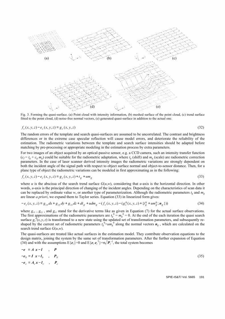
Fig. 3. Forming the quasi-surface. (a) Point cloud with intensity information, (b) meshed surface of the point cloud, (c) trend surfacefitted to the point cloud, (d) noise-free normal vectors, (e) generated quasi-surface in addition to the actual one.

),,(),,(),,( zyxgzyxezyxf ccc =− (32)

The random errors of the template and search quasi-surfaces are assumed to be uncorrelated. The contrast and brightnessdifferences or in the extreme case specular reflection will cause model errors, and deteriorate the reliability of theestimation. The radiometric variations between the template and search surface intensities should be adapted beforematching by pre-processing or appropriate modeling in the estimation process by extra parameters.For two images of an object acquired by an optical-passive sensor, e.g. a CCD camera, such an intensity transfer function(cf = tg + cg mg) could be suitable for the radiometric adaptation, where tg (shift) and mg (scale) are radiometric correctionparameters. In the case of laser scanner derived intensity images the radiometric variations are strongly dependent onboth the incident angle of the signal path with respect to object surface normal and object-to-sensor distance. Then, for aplane type of object the radiometric variations can be modeled in first approximating as in the following:

ggccc umtzyxgzyxezyxf ++=− ),,(),,(),,( (33)

where u is the abscissa of the search trend surface G(u,w), considering that u-axis is the horizontal direction. In otherwords, u-axis is the principal direction of changing of the incident angles. Depending on the characteristics of scan data itcan be replaced by ordinate value w, or another type of parameterization. Although the radiometric parameters tg and mgare linear a priori, we expand them to Taylor series. Equation (33) in linearized form gives:

}));{),,((),,((),,( 000gggccggczcycxc umtzyxgzyxfudmdtdzgdygdxgzyxe n++−−++++=− (34)

where gcx , gcy , and gcz stand for the derivative terms like as given in Equation (7) for the actual surface observations.The first approximations of the radiometric parameters are tg

0 = mg0 = 0. At the end of the each iteration the quasi search

surface gc0(x, y, z) is transformed to a new state using the updated set of transformation parameters, and subsequently re-

shaped by the current set of radiometric parameters tg0+umg

0 along the normal vectors ng , which are calculated on thesearch trend surface G(u,w).The quasi-surfaces are treated like actual surfaces in the estimation model. They contribute observation equations to thedesign matrix, joining the system by the same set of transformation parameters. After the further expansion of Equation(34) and with the assumptions E{ec}=0 and E{ec ec

T}=σ02Pc

-1, the total system becomes

P lxAe ,−=−

bbb P lxIe ,−=− (35)

cccc P lxAe ,−=−

(a) (b) (c)

(d) (e)

SPIE-IS&T/ Vol. 5665 191

where ec , Ac , and Pc are the true error vector, the design matrix, and the associated weight coefficient matrix for thequasi-surface observations respectively, and lc is the constant vector that contains the Euclidean distances between thetemplate and correspondent search quasi-surfaces elements. The hybrid system in Equation (35) is of the combinedadjustment type that allows simultaneous matching of geometry and intensity.In our experiments, weights for the quasi-surface observations are selected as (Pc)ii < (P)ii , and the intensitymeasurements of the (laser) sensor are considered to be uncorrelated with the distance measurements (E{ec eT}=0) for thesake of simplicity of the stochastic model.

4. EXPERIMENTAL RESULTS

Two practical examples are given to show the capabilities of the method. All experiments were carried out using ownself-developed C/C++ software that runs on Microsoft Windows® OS. In all experiments the initial approximations ofthe unknowns were provided by interactively selecting 3 common points on both surfaces before matching. Since in alldata sets there was no scale difference, the scale factor m was fixed to unity by infinite weight value ((Pb)ii → ∞). Theiteration criteria values ci were selected as 1.0e-4 meters for the elements of the translation vector and 1.0e-3 gon for therotation angles.The first example is the registration of three point clouds of a plant (Fig. 4). The scanning was performed by the HDS2500 (Leica Geosystems) laser scanner. The average point spacing is 12 millimeters. The point clouds Fig. 4-a and 4-cwere matched to Fig. 4-b by use of the LS3D surface matching. In this experiment the whole overlapping areas werematched. The numerical results of the matching of the first and third point clouds are given at parts I and II of Table 1respectively. Even though it is a very complex environment, the matching process is quite successful. Relativelyhomogeneous and small magnitudes of the theoretical precisions of the parameters show an excellent fit along alldirections. However the theoretical precisions are too optimistic.

(a) (b) (c)

(d)

Fig. 4. Example “plant”. (a), (b), (c) First, second and third point cloud, (d) composite point cloud after the LS3D surface matching.Note that laser scanner derived intensities are back-projected onto the point clouds.

192 SPIE-IS&T/ Vol. 5665

Table 1: Numerical results of “plant” example

# surf.mode ∑points Iter. 0σ̂ tztytx σσσ ˆ/ˆ/ˆ κϕω σσσ ˆ/ˆ/ˆ

(mm) (mm) (1.0e-02 gon)I P 245041 6 2.78 0.03 / 0.03 / 0.01 0.01 / 0.01 / 0.03

B 5 2.79 0.03 / 0.03 / 0.01 0.01 / 0.01 / 0.03II P 323936 7 2.54 0.02 / 0.02 / 0.01 0.01 / 0.01 / 0.02

B 6 2.52 0.02 / 0.02 / 0.01 0.01 / 0.01 / 0.02III P 20407 6 2.11 0.09 / 0.09 / 0.04 0.05 / 0.04 / 0.08

B 5 2.09 0.09 / 0.09 / 0.04 0.05 / 0.04 / 0.08IV P 37983 8 2.01 0.04 / 0.04 / 0.02 0.03 / 0.03 / 0.07

B 8 2.00 0.04 / 0.05 / 0.02 0.03 / 0.03 / 0.07P: plane surface representation, B: bi-linear surface representation

(a) (b) (c)

(d)Fig. 5. Example “Neuschwanstein”. (a) Left point cloud, (b) right point cloud, (c) coverage of the template patch (inner quadrangle)and the search patch (outer quadrangle), which are selected on the left and right point clouds respectively, (d) composite point cloudafter the simultaneous matching of geometry and intensity by LS3D. Note that laser scanner derived intensities are back-projectedonto the point clouds.

A further matching process was carried outusing the simultaneous multi-subpatchapproach of the LS3D. For the first point cloud5 and for the third point cloud 7 occlusion-freecooperative subpatches were selected. Theresults of the matching of the first and thirdpoint clouds are given at parts III and IV ofTable 1 respectively. Although the precisionvalues increase while the system redundancydecreases, they are still optimistic mainly dueto the stochastic properties of the searchsurfaces.

SPIE-IS&T/ Vol. 5665 193

The second experiment refers to simultaneous matching of surface geometry and intensity. Two scans of a wall paintingin Neuschwanstein Castle in Bavaria, Germany, were matched (Fig. 5). The scanning was performed using the IMAGER5003 (Zoller+Fröhlich) laser scanner. The average point spacing is 3 millimeters. Laser scanner derived reflectancevalues were used as intensity information. The actual surface observations are considered as the unit weight (P)ii=1.Consequently weights for the quasi-surface observations are selected as (Pc)ii=0.75. The iteration criteria values ci wereselected as 2.0e-4 meters for the elements of the translation vector and 5.0e-3 gon for the rotation angles. The searchsurface, selected on the right point cloud, was matched to the template one, which was selected on the left point cloud(Fig. 5-c). The numerical results are given in Table 2.

Table 2: Numerical results of “Neuschwanstein” example

# surf.mode datum ∑points Iter. RMSE tztytx σσσ ˆ/ˆ/ˆ κϕω σσσ ˆ/ˆ/ˆ

(mm) (mm) (1.0e-02 gon)V P f/g 45652 14 1.16 0.26 / 0.06 / 0.07 0.15 / 0.16 / 0.53

B f/g 12 1.18 0.26 / 0.06 / 0.07 0.15 / 0.16 / 0.53VI P F/G 45652 12 1.16 0.25 / 0.06 / 0.07 0.15 / 0.15 / 0.50

B F/G 12 1.18 0.25 / 0.06 / 0.07 0.15 / 0.15 / 0.50f/g: datum are the actual surfaces f /g(x, y, z), F/G: datum are the trend surfaces F/G(u,w)RMSE: root mean square error of the residuals of the actual surface observations

5. CONCLUSIONS

An algorithm for the least squares matching of overlapping 3D surfaces is presented. Our proposed method, the LeastSquares 3D Surface Matching (LS3D), estimates the transformation parameters between two or more fully 3D surfaces,using the Generalized Gauss Markoff model, minimizing the sum of squares of the Euclidean distances between thesurfaces. The mathematical model is a generalization of the least squares image matching method and offers highflexibility for any kind of 3D surface correspondence problem. The least squares concept allows for the monitoring of thequality of the final results by means of precision and reliability criterions. By appropriately selecting the 3Dtransformation method and the surface representation type, it is able to match multi-resolution, multi-temporal, multi-scale, and multi-sensor data sets.The capabilities of the technique are illustrated by a practical example. There are several ways to extend the technique.Here we give two of them, which are simultaneous matching of surface geometry and intensity under a combinedestimation model and simultaneous multi-subpatch matching. Future studies will include more practical examples todemonstrate the full power of the technique.The technique can be applied to a great variety of data co-registration problems. Since it reveals the sensor noise leveland accuracy potential of any kind of surface measurement method or device, it can be used for comparison andvalidation studies. In addition time dependent (temporal) variations of the object surface can be inspected, tracked, andlocalized using the statistical analysis tools of the method.

ACKNOWLEDGEMENTS

The laser scanner data set “plant” is courtesy of Leica Geosystems HDS Inc., and data set “Neuschwanstein” is courtesyof Zoller+Fröhlich GmbH Elektrotechnik. The first author is financially supported by an ETH-Zurich Internal ResearchGrant, which is gratefully acknowledged.

REFERENCES

1. P.J. Besl, N.D. McKay, A method for registration of 3D shapes. IEEE Trans. Pattern Anal. Mach. Intel., 14(2), 239-256, 1992.2. Y. Chen, G. Medioni, Object modelling by registration of multiple range images. Img. and Vis. Comp., 10(3), 145-155, 1992.3. Z. Zhang, Iterative point matching for registration of free-form curves and surfaces. Int. J. of Comp. Vis., 13(2), 119-152, 1994.4. A. Fusiello, U. Castellani, L. Ronchetti, V. Murino, Model acquisition by registration of multiple acoustic range views. Computer

Vision – ECCV 2002, LNCS, vol. 2351, Springer, 805-819, 2002.5. T. Masuda, N. Yokoya, A robust method for registration and segmentation of multiple range images. Comp. Vis. and Img.

Under., 61(3), 295-307, 1995.

Since the object is a plane, onlysurface geometry is not enough for thematching. Using the combinedmatching of surface geometry andintensity approach of the LS3D asuccessful solution has been achieved.The datum as the trend surface optiongives a better convergence rate.

194 SPIE-IS&T/ Vol. 5665

6. R. Bergevin, M. Soucy, H. Gagnon, D. Laurendeau, Towards a general multi-view registration technique. IEEE Trans. PatternAnal. Mach. Intel., 18(5), 540-547, 1996.

7. V. Sequeira, K. Ng, E. Wolfart, J.G.M. Goncalves, D. Hogg, Automated reconstruction of 3D models from real environments.ISPRS J. of Photog. & Rem. Sensing, 54(1), 1-22, 1999.

8. M. Potmesil, Generating models of solid objects by matching 3D surface segments. Int. Joint Conf. on Artificial Intelligence,Karlsruhe, 1089-1093, 1983.

9. C. Dorai, J. Weng, A.K. Jain, Optimal registration of object views using range data. IEEE Trans. Pattern Anal. Mach. Intel.,19(10), 1131-1138, 1997.

10. I.S. Okatani, K. Deguchi, A method for fine registration of multiple view range images considering the measurement errorproperties. Comp. Vis. and Img. Under., 87(1-3), 66-77, 2002.

11. O. Jokinen, H. Haggren, Statistical analysis of two 3-D registration and modeling strategies. ISPRS J. of Photog. & Rem.Sensing, 53(6), 320-341, 1998.

12. J.A. Williams, M. Bennamoun, S. Latham, Multiple view 3D registration: A review and a new technique. IEEE Int. Conf.Systems, Man, and Cybernetics, Tokyo, 497-502, 1999.

13. R.J. Campbell, P.J. Flynn, A survey of free-form object representation and recognition techniques. Comp. Vis. and Img. Under.,81(2), 166-210, 2001.

14. P.J. Neugebauer, Reconstruction of real-world objects via simultaneous registration and robust combination of multiple rangeimages. Int. J. of Shape Modeling, 3(1-2), 71-90, 1997.

15. R. Szeliski, S. Lavallee, Matching 3-D anatomical surfaces with non-rigid deformations using octree-splines. Int. J. of Comp.Vis., 18(2), 171-186, 1996.

16. A. Gruen, Adaptive least squares correlation: a powerful image matching technique. South Afr. J. of Photog., Rem. Sensing andCartography, 14(3), 175-187, 1985.

17. H. Ebner, F. Mueller, Processing of Digital Three Line Imagery using a generalized model for combined point determination. Int.Arch. of Photog. and Rem. Sensing, 26(3/1), 212-222, 1986.

18. H. Ebner, G. Strunz, Combined point determination using Digital Terrain Models as control information. Int. Arch. of Photog.and Rem. Sensing, 27(B11/3), 578-587, 1988.

19. D. Rosenholm, K. Torlegard, Three-dimensional absolute orientation of stereo models using Digital Elevation Models. Photog.Eng. & Rem. Sensing, 54(10), 1385-1389, 1988.

20. G.E. Karras, E. Petsa, DEM matching and detection of deformation in close-range Photogrammetry without control. Photog.Eng. & Rem. Sensing, 59(9), 1419-1424, 1993.

21. L. Pilgrim, Robust estimation applied to surface matching. ISPRS J. of Photog. & Rem. Sensing, 51(5), 243-257, 1996.22. H.L. Mitchell, R.G. Chadwick, Digital Photogrammetric concepts applied to surface deformation studies. Geomatica, 53(4), 405-

414, 1999.23. Z. Xu, Z. Li, Least median of squares matching for automated detection of surface deformations. Int. Arch. of Photog. and Rem.

Sensing, 33(B3), 1000-1007, 2000.24. H.G. Maas, Least-Squares Matching with airborne laserscanning data in a TIN structure. Int. Arch. of Photog. and Rem.

Sensing, 33(3A), 548-555, 2000.25. Y. Postolov, A. Krupnik, K. McIntosh, Registration of airborne laser data to surfaces generated by Photogrammetric means. Int.

Arch. of Photog. and Rem. Sensing, 32(3/W14), 95-99, 1999.26. S. Weik, Registration of 3-D partial surface models using luminance and depth information. IEEE Int. Conf. 3D Digital Imaging

and Modeling, Ottawa, 93-100, 1997.27. A.E. Johnson, S.B. Kang, Registration and integration of textured 3D data. Img. and Vis. Comp., 17(2), 135-147, 1999.28. H.G. Maas, On the use of pulse reflectance data for laserscanner strip adjustment. Int. Arch. of Photog. and Rem. Sensing,

34(3/W4), 2001.29. J. Vanden Wyngaerd, L. Van Gool, Combining texture and shape for automatic crude patch registration. IEEE Int. Conf. 3D

Digital Imaging and Modeling, Banff, 179-186, 2003.30. A. Gruen, Least squares matching: a fundamental measurement algorithm. In: K. Atkinson (ed.), Close Range Photogrammetry

and Machine Vision, Whittles, 217-255, 1996.31. H.G. Maas, A high-speed solid state camera system for the acquisition of flow tomography sequences for 3D least squares

matching. Int. Arch. of Photog. and Rem. Sensing, 30(5), 241-249, 1994.32. H.G. Maas, A. Gruen, Digital photogrammetric techniques for high resolution three dimensional flow velocity measurements.

Opt. Eng., 34(7), 1970-1976, 1995.33. A. Gruen, Photogrammetrische Punktbestimmung mit der Buendelmethode. IGP ETH Zurich, Mitteilungen Nr.40, 1986.34. G.J. Peters, Interactive computer graphics application of the parametric bi-cubic surface to engineering design problems. In:

Computer Aided Geometric Design, Academic Press, 259-302, 1974.35. A. Gruen, E.P. Baltsavias, Geometrically Constrained Multiphoto Matching. Photog. Eng. & Rem. Sensing, 54(5), 633-641,

1988.

SPIE-IS&T/ Vol. 5665 195