a fluid mechanical view on abdominal aortic aneurysms
TRANSCRIPT
HAL Id: hal-00998006https://hal-polytechnique.archives-ouvertes.fr/hal-00998006
Submitted on 8 Jul 2014
HAL is a multi-disciplinary open accessarchive for the deposit and dissemination of sci-entific research documents, whether they are pub-lished or not. The documents may come fromteaching and research institutions in France orabroad, or from public or private research centers.
L’archive ouverte pluridisciplinaire HAL, estdestinée au dépôt et à la diffusion de documentsscientifiques de niveau recherche, publiés ou non,émanant des établissements d’enseignement et derecherche français ou étrangers, des laboratoirespublics ou privés.
A fluid mechanical view on abdominal aortic aneurysmsV. Duclaux, F. Gallaire, Christophe Clanet
To cite this version:V. Duclaux, F. Gallaire, Christophe Clanet. A fluid mechanical view on abdominal aorticaneurysms. Journal of Fluid Mechanics, Cambridge University Press (CUP), 2010, 664, pp.5-32.10.1017/s0022112010003782. hal-00998006
J. Fluid Mech. (2010), vol. 664, pp. 5–32. c© Cambridge University Press 2010
doi:10.1017/S0022112010003782
5
A fluid mechanical view on abdominalaortic aneurysms
VIRGINIE DUCLAUX1, FRANCOIS GALLAIRE2,AND CHRISTOPHE CLANET3†
1IRPHE, UMR 6594, 49 rue F. Joliot-Curie, 13384 Marseille, France2LFMI, Ecole Polytechnique Federale de Lausanne, 1015 Lausanne, Switzerland
3LadHyX, UMR 7646, Ecole Polytechnique, 91178 Palaiseau, France
(Received 22 September 2008; revised 7 July 2010; accepted 12 July 2010)
Abdominal aortic aneurysms are a dilatation of the aorta, localized preferentiallyabove the bifurcation of the iliac arteries, which increases in time. Understandingtheir localization and growth rate remain two open questions that can have either abiological or a physical origin. In order to identify the respective role of biologicaland physical processes, we address in this article these questions of the localizationand growth using a simplified physical experiment in which water (blood) is pumpedperiodically (amplitude a, pulsation ω) in an elastic membrane (aorta) (length L, cross-section A0 and elastic wave speed c0) and study the deformation of this membranewhile decharging in a rigid tube (iliac artery; hydraulic loss K). We first showthat this pulsed flow either leads to a homogenous deformation or inhomogenousdeformation depending on the value of the non-dimensional parameter c2
0/(aLω2K).These different regimes can be related to the aneurysm locations. In the second part,we study the growth of aneurysms and show that they only develop above a criticalflow rate which scales as A0c0/
√K .
Key words: biomedical flows, flow–vessel interactions
1. Introduction1.1. Definitions and history
The use of the word aneurysm (dilate in Greek) in medicine seems to go back to Guyde Chauliac (1373), medical doctor of four popes and considered as the ‘father’ ofmediaeval surgery. He used this word in La grande Chirurgie to designate the localdilatation of an artery. The study of aneurysms progressed with the development ofmedical techniques, starting with the stethoscope of Laennec (1819), who writes:
We use aneurysm to designate either the dilation of an artery or the presence of a sack connected to
the artery. The first case is called true aneurysm by surgeons while the second is referred to as false
aneurysm.
We learn from these definitions that aneurysms develop on arteries and can beclassified in two different types which are now called fusiform (‘true’), illustrated infigure 1(b) with an abdominal aortic aneurysm (AAA), and saccular (‘false’) illustrated
† Email address for correspondence: [email protected]

6 V. Duclaux, F. Gallaire and C. Clanet
(a) (b) (c)
1
2
3
4
5
6
7
Figure 1. (Colour online) (a) Three-dimensional angiography of an aorta without aneurysm:(1) heart, (2) aortic arch, (3) coronary arteries, (4) thoracic aorta, (5) kidneys, (6) abdominalaorta and (7) iliac arteries. (b) Angiography of an aorta with an abdominal aortic aneurysm.(c) Angiography of a cerebral aneurysm.
in figure 1(c) with a cerebral aneurysm. We focus on fusiform aneurysms and use asa paradigm the AAA (Roberts 1959; Glagov 1961).
1.2. Physiological characteristics
The main geometrical features of the aorta are presented in figure 1(a): at theexit of the left ventricle, the aortic arch conducts the aorta from the heart to thespinal column. The thoracic and abdominal aortas designate the ‘straight’ portionsof the aorta located above and below the diaphragm, respectively. At the end ofthe spinal column, the aorta splits into two iliac arteries, which irrigate each of thelegs. For humans, the aorta is the longest artery (L ≈ 40 cm) and we observe fromthis angiography that its diameter (D ≈ 2 cm) is much larger than the secondaryconnecting vessels. To a first approximation, the aorta will thus be considered as aplain tube without branching until the iliac arteries.
We observe in figure 1(b) that the AAA develops above the bifurcation of theiliac arteries. According to recent studies (Lasheras 2007), AAA rarely appears inindividuals under 50 years of age, but their incidence increases drastically at the ageof 55 and peaks in the early 80s. A large screening study conducted in Norway in1994–1995 showed that AAA are present in 8.9 % of men and 2.2 % of women over60 years of age.
The exact reasons for the development of AAA are still unknown (Alexander 2004,McAuley et al. 2002). However, atherosclerosis and hypertension have been recognizedas important risk factors. Atherosclerosis can be responsible for the alteration of thewall properties while hypertension can be responsible for the overpressure leading toa local deformation of the aorta.
With regard to the growth rate of the aneurysms and the risk of rupture, theyboth increase with the size of the aneurysm: the study by Guirguis & Barber (1991),dedicated to the growth after 12 months of four classes of aneurysms (diameters lessthan 4 cm, from 4 to 5 cm, from 5 to 6 cm and more than 6 cm), shows that theyhave grown of 0.2, 0.3, 0.4 and 0.8 cm, respectively. With regard to the risk of rupture,
A fluid mechanical view on abdominal aortic aneurysms 7
the same study reveals that the risk factor for aneurysms of diameters less than 4 cm,from 4 to 5 cm and larger than 5 cm is 1, 2 and 20 %, respectively.
1.3. Physical properties and orders of magnitude
The blood is composed of different cells, the larger ones being the leucocytes(dmax ≈ 22 µm in diameter) and the more numerous being the red blood cells (meandiameter 7 µm, Humphrey & Delange 2004). Depending on the size R0 of the vesselin which the blood is flowing, it can behave either as a Newtonian (R0/dmax 1) or asa non-Newtonian (R0/dmax < 1) liquid (Reinke 1986). In the limit of large vessels suchas the aorta (R0/dmax ≈ 450), the blood behaves as a Newtonian liquid of kinematicviscosity ν ≈ 4.10−6 m2 s−1 (Pedley 1980; Chandran & Yearwood 1981; Ku 1997).
The non-intrusive velocity measurements in the human aorta obtained by Chenget al. (2003) using the magnetic resonance imaging (MRI) reveal that the meanvelocity is always smaller than the metre per second (U ≈ 0.8 m s−1) and that thevelocity profile is close to a top hat with thin boundary layers O(1) mm.
The wall of arteries is composed of three layers, the intima, the media and theadventia. The media is composed of elastin, which enables the dilatation of the arterywhen exposed to a transmural pressure increase. For mammals, the order of magnitudeof the pressure variation over a cardiac cycle is of the order of δp ≈ ρgH , where H isthe size of the mammal (McDonald 1960, 1968), which means that δp ≈ 104 Pa for ahuman. The corresponding relative variations of the cross-section of the arteries areof the order of 10 %: δA/A ≈ 0.1. To describe the elastic behaviour of the arteries,the physiologists use the distensibility D ≡ A−1δA/δp, which can be evaluated using
the previous estimations to 10−5 m2 N−1
for a human (McDonald 1968; Fung 1990).Lighthill (1975) showed that this deformation can be localized and can propagatewithout dispersion along the aorta with the wave speed c0 = 1/
√ρD ≈ 10 m s−1, much
larger than the flow velocity.To model the aortic flow in a laboratory experiment, one needs to respect the
non-dimensional numbers which characterize the actual flow. For a Newtonian liquidflowing in a tube of radius R0 with the mean velocity U , the flow is first characterizedby the Reynolds number Re ≡ UR0/ν ≈ 103, which compares inertial effects (ρR2
0U2)
to viscous forces ρνUR0. In this limit of high Reynolds numbers, inertia dominatesand viscous effects are concentrated in thin boundary layers close to the walls.
In the case of a pulsating flow (pulsation ω), Stokes’ second problem gives a scalingof the boundary layer size δ ≈
√ν/ω. The ratio R0/δ gives the relative size of the
boundary layer compared with the size of the tube. In physiological applications, thisratio is known as the Womersley number Wo ≡ R0
√ω/ν (Womersley 1957). For the
aorta, we evaluate Wo ≈ 20. The boundary layer is thus small compared with the sizeof the artery, and we recover the observation done considering the plug-like velocityprofiles measured by Cheng et al. (2003).
Finally, since the artery is elastic, one needs to respect the ratio between the elasticwave propagation c0 and the velocity of the flow U . This ratio Sh ≡ U/c0 is classicallycalled the Shapiro number (Paıdoussis 2006). For the aorta Sh ≈ 0.1.
In conclusion, in order to reproduce the physiological flow, the experiment must beconducted in the limit
Re 1, Wo 1, Sh 1. (1.1)
1.4. Objectives
Abdominal aortic aneurysms have been found to be systematically localized beforethe iliac bifurcation and are characterized by a growth rate which increases with their

8 V. Duclaux, F. Gallaire and C. Clanet
W
T
S
ECST
C
P0
P1 P2
L0x
H
M
Ud
a, ω A(x,t)
Figure 2. (Colour online) Sketch of the experiment: T= tank, W= water, ST= stroke(oscillatory motion of the amplitude a and the angular frequency ω), C= computer, S = servo,EC= electrical cylinder, P1 and P2 = pressure sensors and M= elastic membrane. We alsouse d for the local membrane thickness, U for the local flow velocity and A for the localcross-section. Finally, P0 stands for the atmospheric pressure and H is the vertical distancebetween the membrane and the tank.
size and a characteristic period of development of the order of a year. To determinethe respective role of biology and mechanics in AAA, we reproduce, in a scaledmodel, the pulsating flow of a Newtonian liquid in an elastic membrane and identifythe mechanical conditions under which aneurysms can form.
The experimental set-up is presented in § 2. The dynamics of the aorta on the timescale of the heart beat is presented in § 3, where the question of the localization isaddressed. The development and growth rate of the aneurysms is addressed in § 4,prior to the conclusion in § 5.
2. Experimental set-up and protocolIn this section, we first give an overview of the experiment and then detail each of
the main parts before presenting the diagnostic tools used to quantify the dynamicsof the deformation of the membrane.
2.1. Overview
The experimental set-up is sketched in figure 2: the water (blood) (W) is containedin a tank (T) with a free surface maintained at the constant atmospheric pressureP0. Using a computer (C) we move, via the servo (S), an electric cylinder (EC) whichpumps the water in the stroke (heart) (ST) with the amplitude a and the frequencyω. We define the amplitude with respect to the liquid motion at the exit of the stroke,which means that the velocity of the liquid as it enters the membrane (aorta) (M)is of the order of aω. Two valves in the stroke impose the motion of the liquid inthe anticlockwise direction as indicated by the arrows. Two pressure sensors (P1) and(P2) enable the measure of the pressure variation across the membrane. At the exitof the elastic membrane, the liquid returns to the tank via a rigid tube (iliac artery).The tank is located above the membrane, at a height H ≈ 1 m which imposes a meanpressure jump across the membrane of the order of ρgH . This positive pressure jumpensures that as long as the velocity in the membrane remains smaller than
√2gH ,

A fluid mechanical view on abdominal aortic aneurysms 9
L R0 ≡√
A0/π d0 c0 E
(cm) (mm) (mm) (m s−1) (MPa)
Elastin: 2.4Human aorta 40 7.4–11.3 ≈1 5.15; 6 Collagen: 114(Fung 1997; Global: 5.3Groenink et al. 1999)Latex membrane 0–200 9.5 0.7 6 1.07Michelin
Human iliac artery 5 ≈ 5.5 ≈ 0.7 9 ; 11.5 Global: 10(Gray 1918; Li et al. 1981;Medynsky et al. 1998)
Table 1. Characteristics of human arteries and latex membrane.
the membrane is always under tension. Since arteries work in this inflated regime, thewhole study is conducted in this limit.
2.2. An elastic membrane for the aorta
As an elastic membrane, we have used latex tyre tubes from Michelin, the propertiesof which are presented in table 1 and compared with the properties of the humanaorta and iliac arteries. The elastic membrane is characterized by its length L, initialunstretched cross-section A0, initial thickness d0 and Young modulus E. We alsoreport in table 1 the value of the elastic wave speed c0 ≡
√d0 E/2ρR0 (Lighthill 1975),
defined with ρ as the density of the contained liquid and R0 ≡√
A0/π as the initialradius of the membrane.
Note in table 1 that the geometrical properties (L, R0, d0) as well as the dynamicalcharacteristic (c0) of the latex membrane are compatible with the characteristics ofthe human aorta reported in the literature. We also underline the higher rigidity ofthe iliac artery which is modelled in our experiment using the limit of a rigid tube(see § 2.2.4).
2.2.1. Experimental characterization of the elasticity of the membrane
To characterize the elastic properties of the latex membrane, we have used anhydraulic traction machine, presented in figure 3(a): a rectangular piece of material(length L0, width b0 and thickness h0) is initially clamped between cylindrical jaws.A controlled traction force F is then exerted via the jaws on the membrane andthe corresponding equilibrium length L is measured. The relation between the stressσ ≡ F/(hb) and the relative extension ε ≡ (L − L0)/L0 is presented in figure 3(b).In this graph, the force F and the length L are measured while the cross-sectionhb is deduced from the initial cross-section h0b0 via the incompressibility relationhb = h0 b0 L0/L, which assumes a Poisson coefficient νp =1/2.
In the limit of small relative deformation ε < 2, the stress is proportional to thedeformation σ ≈ 106ε. This is the Hookean regime from which one deduces thevalue of the Young modulus E ≈ 1 MPa presented in table 1. For a higher relativedeformation, the stress is a stronger function of the deformation as plastic effectsappear (Carpenter & Pedley 2003).
2.2.2. A pressure law for the cylindrical membrane
Let us now consider a cylindrical membrane such as the one presented schematicallyin figure 4(a). When there is no pressure jump across the membrane (P = P0) the

10 V. Duclaux, F. Gallaire and C. Clanet
F(a) (b)
F
h
108
σ =
F/h
b (P
a)
107
106
105
1040.01 0.1 1 10
b
L
ε = (L – L0)/L0
Figure 3. Characterization of the elastic properties of the membrane: (a) scheme of thetraction experiment, (b) results obtained for the traction stress σ ≡ F/(hb) as a function of therelative elongation ε ≡ (L − L0)/L0.
105
104
103
F
d P
F
P0
Rβ
0.01 0.1 1 10
p (P
a)
R/R0 – 1
p*
(a)
(b)
Figure 4. A pressure law for the cylindrical membrane: (a) scheme for the equilibrium, (b)experimental evolution of the transmural pressure p with the relative deformation R/R0 − 1(). The solid line corresponds to the theoretical curve (2.2).
radius of the membrane is R0. When the pressure across the membrane increasesp ≡ P − P0 > 0, the new equilibrium radius R results from the balance between thepressure and elastic stresses. For a small element of the angular extension β , thisequilibrium reads
p =d0
R0
σ (ε)
(1 + ε)2, (2.1)

A fluid mechanical view on abdominal aortic aneurysms 11
f Ejected volume Ω Reynolds no. Womersley no. Shapiro no.(Hz) (cm3 cycle−1) Re = UR0/ν Wo = R
√ω/ν Sh= U/c0
Human heart 1.25–3 ∼80 700–2500 ∼20 0.1–0.25Electric cylinder 0.1–10 5.6–168 900–104 7–40 0.1–0.16
Table 2. Properties of the human heart (Shapiro 1977; Chandran & Yearwood 1981; Fung1990; Ku 1997; Groenink et al. 1999; Humphrey & Delange 2004) and the present experiment.
where ε ≡ R/R0 − 1. The experimental evolution p(R/R0) is shown in figure 4(b)by solid squares. At small relative extensions (ε < 1), the radius of the membraneincreases with the pressure. This evolution stops at R = 2 R0, where the pressurereaches a maximum p ≈ 18 500 Pa. If the pressure is increased above this criticalpressure, one observes a jump on the radius from R =2 R0 to R ≈ 6 R0. For an evenhigher pressure, since the membrane becomes stiffer, the radius increases with a lowersensitivity to the pressure.
Using the Hookean expression of the stress σ = Eε, the pressure–radius equation(2.1) reduces to
p = Ed0
R0
ε
(1 + ε)2. (2.2)
This relation is shown by a thin solid line in figure 4(b). The comparison with theexperimental data shows that the linear Hookean approximation does capture theevolution of the pressure up to the pressure maximum p. It predicts correctlythe extension at which the maximum occurs (dp/dR = 0 when R/R0 = 2) as wellas the absolute value of the critical pressure. Since the Hookean model does notaccount for the stiffening of the membrane at large relative deformations (observed infigure 3b), it fails to describe the increase of the pressure observed in the range ε > 5.However, since the whole study is conducted in the range of deformations R/R0 2,we will use the Hookean approximation (2.2) to describe the pressure–radius relation.In terms of the cross-section A, this relation can be rewritten
p (A) = 2ρc20
(√A0
A− A0
A
). (2.3)
Under this form, the relation has already been used (Paquerot & Lambrakos 1994)and discussed in Olsen & Shapiro (1967). In Olsen & Shapiro (1967), the authorsprefer a pressure law derived from statistical physics given by p = 1/2ρc2
0[1−(A0/A)2].Both expressions are equal in the limit A/A0 = 1 + εA, where p = ρc2
0εA (εA 1).However, the essential difference between the two expressions is that one predicts amaximum (see (2.3)) while the other predicts a saturation. Since the maximum andthe corresponding instability is observed experimentally as shown in figure 4(b) wehave decided to work with the Hookean model (2.3).
2.3. An electrical cylinder for the heart
Concerning the heart, we report in table 2 its main mechanical characteristics: beatfrequency f ≡ ω/2π and ejected volume per beat Ω . These values are comparedwith those obtained artificially from the electric cylinder (IDC-Motion EC3-B23)controlled with a computer. Both the frequency and the ejected volume range of thephysiological system are covered by the experimental counterpart. These parameter

12 V. Duclaux, F. Gallaire and C. Clanet
2×10⁴
1.5×10⁴
U P
P0 5×10³
1×10⁴
0
P –
P0
– ρ
gH (
Pa)
(b)(a)
U2 (m2 s–2)
0.2 0.4 0.6 0.8 1.0 1.2 1.4
H
Figure 5. (Colour online) Resistance to the flow: (a) scheme of the experimental set-updedicated to the description of the resistance, (b) measurement of the pressure in the membranep ≡ P − P0 − ρgH as a function of the square of the mean velocity U 2. The proportionalityp = KρU 2 is illustrated for three different rigid tubes which lead to K = 8 (), K =14 ( )and K = 40 ( ).
ranges have been chosen to generate a flow in the elastic membrane in close similaritywith that observed in the aorta.
The similarity between both flows is achieved by using similar non-dimensionalnumbers: Reynolds, Womersley and Shapiro numbers. Their typical range ofvariations is indicated in table 2. The Reynolds number Re ≡ UR0/ν = Ωf/πR0ν
is typically O(103) in the human aorta (Chandran & Yearwood 1981; Fung 1990;Groenink et al. 1999) whereas the range of the experiment is 900–104. The Womersleynumber Wo ≡ R0/
√ν/ω is O(20) in the aorta (Fung 1990; Ku 1997; Humphrey &
Delange 2004) and ranges between 7 and 40 in our experiment. Finally, the Shapironumber Sh ≡ U/c0 compares the velocity of the flow to the propagation velocity ofthe elastic waves on the aorta. The Shapiro number is small in the aorta (typically0.1, Pedley 1980) and the same range is achieved in our experiment.
2.4. A rigid tube as iliac artery
As seen in table 1 and mentioned in § 2.2, the iliac arteries are stiffer than the aorta.Moreover, the network of subsequent arteries and vessel behaves as a ‘resistance’ forthe flow in the aorta (McDonald 1960). To model these two effects, we connect theelastic membrane to a rigid tube the diameter (and length) of which is used to changethe ‘resistance’ to the flow. Experimentally, this connection is achieved using a hoseclamp.
In analogy with Ohm’s law, the resistance is classically defined as the relationbetween the pressure and the velocity in the membrane.
To measure this resistance, we have conducted a specific experiment presented infigure 5(a): first, the elastic membrane is filled with water and set into tension by astatic pressure Ps ≡ P0+ρgH imposed by the rigid tube which connects the membraneto an overflow standing at a height H above the elastic tube. A mean velocity U isthen imposed and we measure the corresponding pressure difference p ≡ P −Ps . Theevolution p(U ) is presented in figure 5(b). We observed a linear relation between thepressure difference and the square of the mean velocity: p = KρU 2. The constantof proportionality K changes from 8 to 14 and then 40 as we have varied the rigidtube length and diameter. Since the Reynolds number of the flow in the experiment

A fluid mechanical view on abdominal aortic aneurysms 13
Membrane
Laser diode δx δx
δRδRα
(a) (b) (c)
Figure 6. Experimental method used to measure the deformation of the membrane: (a)scheme of the set-up, (b) example of the observation in the case of a homogeneous deformation,(c) example of the observation in the case of an inhomogeneous deformation.
is large (>103), one is not surprised to obtain such a relationship for the resistance(Prandtl & Tietjens 1957).
Furthermore, with a mean velocity of the order of the metre per second, thecorresponding pressure losses for the three different resistances are 8000, 14 000 and40 000 Pa. These values are comparable to the pressure loss measured in a humanaorta, ≈ 104 Pa (McDonald 1960).
2.5. Experimental methods
In the limit of small deformations, the law of the membrane (2.3) shows that therelative deformation δR/R0 is related to the pressure fluctuations δp via the relationδR/R0 ∼ δp/ρc2
0. The evaluation δp ∼ ρU 2 leads to δR/R0 ∼ (U/c0)2 ≈ 1–10 %. For
a centimetric elastic membrane (c0 ≈ 6 m s−1) and a typical metre per second flow, wededuce that the radial deformations are millimetric. Since the length of the aorta isof the order of 1 m, the ratio between the length scale of the domain and the lengthscale of the deformation is 103. This is out of the scope of a classical video camera∼102. We thus use a geometrical magnification to reduce the scale ratio to 102 inorder to observe the dynamical deformations of the membrane with a video camera.This geometrical zoom is presented in figure 6(a): it consists of a comb of lasersheets inclined of an angle α with respect to the membrane. As shown in figure 6(b,c),each laser sheet intersects the cylindrical membrane and produces a bright ellipticaltrace. In figure 6(b,c), the image at the top represents the membrane prior to thedeformation (the edges of the membrane are marked by long dashed lines) whilethe image at the bottom presents the membrane after the deformation (the edges ofthe membrane after the deformation are underlined by short dashed lines). The radialdeformation being millimetric δR ≈ 1 mm, we observed that it induces a displacementof the laser trace δx ≈ 1 cm. The geometrical relation between the two variationsis δx =2δR/ tan α. The displacements are reduced to a translation in the case of ahomogeneous deformation (figure 6b) or lead to a more complex figure in the caseof an inhomogeneous deformation (figure 6c).
3. Dynamics on the time scale of the heart beatIn this section, we consider the dynamics of the deformation of the elastic
membrane on the time scale of a few periods of forcing. We first present theexperimental results and then the model and numerics are developed to account for theobservations.

14 V. Duclaux, F. Gallaire and C. Clanet
(a)
(b) (c)0 0
6 st
5.9 st
1 m
x x
1 m
Figure 7. Spatio-temporal diagrams: (a) view from above of the whole membrane L = 1 m,R0 = 1 cm; (b) spatio-temporal diagram obtained during 6 s at the frequency f =0.5 Hz withthe amplitude a = 270 mm; (c) spatio-temporal diagram obtained during 5.9 s at the frequencyf = 3 Hz with the amplitude a =45 mm.
3.1. Experimental evidence of two distinct regimes
The experimental results presented in this section have all been obtained with theresistance (of the iliac artery): K = 8. In order to describe the time evolution of thedeformation of the membrane, we use spatio-temporal diagrams: starting from aglobal view of the membrane such as the one presented in figure 7(a) we extractthe centred horizontal line and construct a new image where its different linescorrespond to the selected line at different times equally spaced. An example of sucha spatio-temporal diagram is presented in figure 7(b). This diagram extends over 6 sand corresponds to the experimental conditions: f =0.5 Hz, amplitude a = 270 mm(velocity aω =0.85 m s−1). At a given spatial location we observe that the deviationof the light oscillates in time with the period of ≈2 s. We also measure an amplitudeof the deviation of ≈ 1 cm which implies a radius variation δR ≈ 1 mm.
Considering the spatial evolution of the deviations, figure 7(b) presents asynchronous translation of the different beams: the membrane thus undergoes anhomogeneous deformation. Let us now consider the spatio-temporal diagram shownin figure 7(c) obtained at the same velocity (0.85 m s−1) but with different forcingconditions: f =3 Hz and a = 45 mm. The time evolution of the light deviation at agiven location contains more harmonics than in figure 7(b). Furthermore, instead of asynchronous translation of the beams, we observe strong oscillations at the entranceand the exit of the membrane and almost no oscillations at an intermediate positionx ≈ 0.6 m. We also observe that the oscillations at the two ends oscillate out of phase.
We retain from the qualitative analysis of these spatio-temporal diagrams thatdepending on the value of the forcing parameters, the membrane can undergo eitheran homogeneous deformation or an inhomogeneous one.
The transition between the two regimes of deformation illustrated in figures 7(b)and 7(c) can be quantified. First, keeping the length of the membrane constant(L =50 cm), figure 8(a) shows the evolution of the critical amplitude of forcing a
with the frequency f . As the frequency increases from 0.65 to 1.5 Hz, the critical

A fluid mechanical view on abdominal aortic aneurysms 15
0
50
100
150
200
250
300(a) (b)
0.2 0.4 0.6 0.8 1.0 1.2 1.4 1.6
f * (Hz) f * (Hz)
a* (m
m)
L*
(cm
)
0
10
20
30
40
50
60
1 2 3 4 5
Inhomogeneous
Homogeneous
L = 50 cm a = 27 mm
Inhomogeneous
Homogeneous
Figure 8. Quantitative analysis of the transition between the homogeneous andinhomogeneous deformation regimes: (a) evolution of the critical amplitude a (denotedby solid squares) with the frequency f for a fixed length of the membrane L = 50 cm; (b)evolution of the critical length L (denoted by solid squares) as a function of the frequency f
for a fixed amplitude a =27 mm.
Qin(t) Qout(t)Ω(t)A(t)
L
Figure 9. Windkessel model: Qin(t) is the inlet flow rate, Qout (t) is the outlet flow rate, Ω(t)is the volume of the fluid contained in the membrane and A(t) is the mean cross-section.
amplitude above which an inhomogeneous membrane is observed decreases from 270to 27 mm.
Now keeping the amplitude of forcing constant (a = 27 mm), figure 8(b) displaysthe evolution of the critical length L as a function of the forcing frequency f . Ata given frequency, we observe an homogeneous deformation on ‘short’ membranesand an inhomogeneous deformation above L. As f increases from 1.5 to 4 Hz, thecritical length decreases from 50 to 10 cm.
3.2. Model
To discuss the homogeneous character of the deformation, we first consider theWindkessel model (Frank 1905) which consists of a lumped (space averaged) modelof the flow in the elastic membrane as shown in figure 9. In this limit, the cross-sectionof the membrane only depends on time through mass conservation which reads
LdA
dt= Qin(t) − Qout (t). (3.1)
In this equation, Qin(t) is imposed by the ‘heart’ while Qout (t) is related to the pressurep in the membrane via the relation
Qout (t) = Aout
√p
Kρ, (3.2)
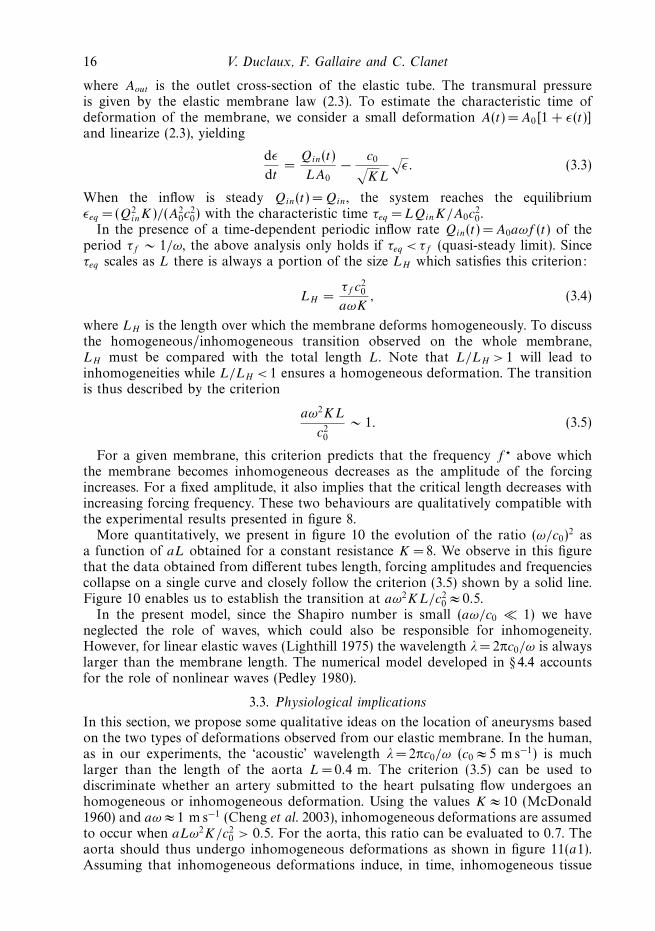
16 V. Duclaux, F. Gallaire and C. Clanet
where Aout is the outlet cross-section of the elastic tube. The transmural pressureis given by the elastic membrane law (2.3). To estimate the characteristic time ofdeformation of the membrane, we consider a small deformation A(t) = A0[1 + ε(t)]and linearize (2.3), yielding
dε
dt=
Qin(t)
LA0
− c0√KL
√ε. (3.3)
When the inflow is steady Qin(t) = Qin, the system reaches the equilibriumεeq = (Q2
inK)/(A20c
20) with the characteristic time τeq = LQinK/A0c
20.
In the presence of a time-dependent periodic inflow rate Qin(t) = A0aωf (t) of theperiod τf ∼ 1/ω, the above analysis only holds if τeq < τf (quasi-steady limit). Sinceτeq scales as L there is always a portion of the size LH which satisfies this criterion:
LH =τf c2
0
aωK, (3.4)
where LH is the length over which the membrane deforms homogeneously. To discussthe homogeneous/inhomogeneous transition observed on the whole membrane,LH must be compared with the total length L. Note that L/LH > 1 will lead toinhomogeneities while L/LH < 1 ensures a homogeneous deformation. The transitionis thus described by the criterion
aω2KL
c20
∼ 1. (3.5)
For a given membrane, this criterion predicts that the frequency f above whichthe membrane becomes inhomogeneous decreases as the amplitude of the forcingincreases. For a fixed amplitude, it also implies that the critical length decreases withincreasing forcing frequency. These two behaviours are qualitatively compatible withthe experimental results presented in figure 8.
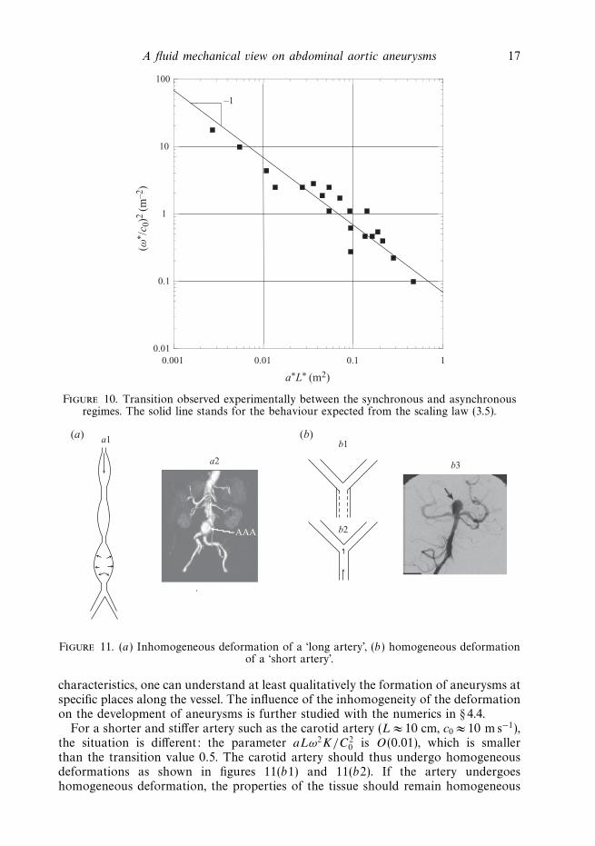
More quantitatively, we present in figure 10 the evolution of the ratio (ω/c0)2 as
a function of aL obtained for a constant resistance K =8. We observe in this figurethat the data obtained from different tubes length, forcing amplitudes and frequenciescollapse on a single curve and closely follow the criterion (3.5) shown by a solid line.Figure 10 enables us to establish the transition at aω2KL/c2
0 ≈ 0.5.In the present model, since the Shapiro number is small (aω/c0 1) we have
neglected the role of waves, which could also be responsible for inhomogeneity.However, for linear elastic waves (Lighthill 1975) the wavelength λ=2πc0/ω is alwayslarger than the membrane length. The numerical model developed in § 4.4 accountsfor the role of nonlinear waves (Pedley 1980).
3.3. Physiological implications
In this section, we propose some qualitative ideas on the location of aneurysms basedon the two types of deformations observed from our elastic membrane. In the human,as in our experiments, the ‘acoustic’ wavelength λ= 2πc0/ω (c0 ≈ 5 m s−1) is muchlarger than the length of the aorta L = 0.4 m. The criterion (3.5) can be used todiscriminate whether an artery submitted to the heart pulsating flow undergoes anhomogeneous or inhomogeneous deformation. Using the values K ≈ 10 (McDonald1960) and aω ≈ 1 m s−1 (Cheng et al. 2003), inhomogeneous deformations are assumedto occur when aLω2K/c2
0 > 0.5. For the aorta, this ratio can be evaluated to 0.7. Theaorta should thus undergo inhomogeneous deformations as shown in figure 11(a1).Assuming that inhomogeneous deformations induce, in time, inhomogeneous tissue
A fluid mechanical view on abdominal aortic aneurysms 17
0.01
0.1
1
10
100
0.001 0.01 0.1 1
–1
a*L* (m2)
(ω* /
c 0)2 (m
–2)
Figure 10. Transition observed experimentally between the synchronous and asynchronousregimes. The solid line stands for the behaviour expected from the scaling law (3.5).
a1
a2
AAA
(a) (b)
b3
b1
b2
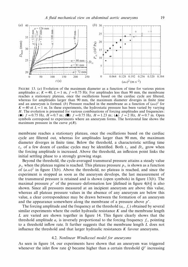
Figure 11. (a) Inhomogeneous deformation of a ‘long artery’, (b) homogeneous deformationof a ‘short artery’.
characteristics, one can understand at least qualitatively the formation of aneurysms atspecific places along the vessel. The influence of the inhomogeneity of the deformationon the development of aneurysms is further studied with the numerics in § 4.4.
For a shorter and stiffer artery such as the carotid artery (L ≈ 10 cm, c0 ≈ 10 m s−1),the situation is different: the parameter aLω2K/C2
0 is O(0.01), which is smallerthan the transition value 0.5. The carotid artery should thus undergo homogeneousdeformations as shown in figures 11(b1) and 11(b2). If the artery undergoeshomogeneous deformation, the properties of the tissue should remain homogeneous

18 V. Duclaux, F. Gallaire and C. Clanet
40
35
30
25
20
15
10
5
0 100 200 300
Location (mm)
Dia
met
er (
mm
)
400 500
Figure 12. Diameter (mm) of the membrane as a function of the position x along themembrane, obtained by two simultaneous experimental diagnostics: a lateral close viewdelivered by a digital camera (reproduced in the figure inlet), and a set of discrete datapoints retrieved from the view from above of the displacement of the laser sheet device. Bothshapes are well fitted by Gaussian functions.
and there is no reason for the appearance of an inhomogeneity along the artery. Inthis limit, if an inhomogeneity appears, it should be observed ‘outside’ the artery. Theaneurysm presented in figure 11(b3) can be seen as an aneurysm developing outsidean artery.
4. Dynamics on the time scale of life4.1. Experimental observations
The time required for the development of an AAA is of the order of years and,therefore, of the order of millions of cardiac cycles. The aim of this section is toanalyse if similar growing processes can be identified in our experiment and underwhich circumstances saturation is encountered or catastrophic growth (aneurysm)triggered.
In order to detect and characterize growing bulges on the membrane and to measurethe precise membrane shape as a function of time and space, the laser sheet devicedescribed in § 2 is used.
When a small deformation occurs as in the case shown in figure 12, the discreteset of data points is fitted by a Gaussian function of the form D(x, t) = Db(t) +D(t) exp[−(x − xc(t))
2/δ(t)2], where Db(t) is the base diameter away from the bulge,D(t) is the bulge amplitude, xc(t) is the bulge centre position, and δ(t) is the bulgewidth. An alternative determination is obtained through a fit of a lateral close viewdelivered by a digital camera, as seen in the inset of figure 12, where the two fitsare shown in the same graph at a given time. Both fitting functions agree to acertain extent, 24.5 + 3.64 exp[−(x − 205.45)2/820] for the imaging technique and24.32 + 4.29 exp[−(x − 201.79)2/490] for the best fit over the laser deviations. Thesediscrepancies are related not only to the experimental techniques but also to thepresence of the bottom wall which breaks the axisymmetry. In this example, therelative discrepancy on the maximum diameter Dmax = Db + D is less than 1 %. Inthe sequel, the laser sheet device is used for determining the above shape parameters.
The long time (over more than 100 ‘cardiac’ periods) evolution of the maximumdiameter for K = 40, L = 1 m and f = 0.75 Hz is shown in figure 13(a) for variousforcing amplitudes a. A threshold is visible: For amplitudes less than 90 mm, the
A fluid mechanical view on abdominal aortic aneurysms 19
40 30
25
20
15
10
5
0
Dm
ax (
mm
)(a) (b)
P∞
(103
Pa)
D∞
35
30
25
20
50
a =
135
mm
a =
117
mm
a = 126 mm
a = 90 mm
a = 72 mm
a = 81 mm
a =
108
mm
a =
99
mm
100 150
t (s) (aω)2 (m s–2)
200 250 0.064 0.128 0.192 0.256 0.320 0.3840
Figure 13. (a) Evolution of the maximum diameter as a function of time for various pistonamplitudes a; K =40, L = 1 m, f = 0.75 Hz. For amplitudes less than 90 mm, the membranereaches a stationary plateau, once the oscillations based on the cardiac cycle are filtered,whereas for amplitudes larger than 90 mm, the maximum diameter diverges in finite timeand an aneurysm is formed. (b) Pressure reached in the membrane as a function of (aω)2 forK = 40 et L = 1 m. In these experiments, the hydrostatic pressure has been varied by varyingH . The evolution is presented for various combinations of forcing amplitudes and frequencies:() f = 0.75 Hz, H =0.7 m; () f = 0.75 Hz, H = 1.23 m; () f =2 Hz, H = 0.7 m. Opensymbols correspond to experiments where an aneurysm forms. The horizontal line shows themaximum pressure in the curve p(R).
membrane reaches a stationary plateau, once the oscillations based on the cardiaccycle are filtered out, whereas for amplitudes larger than 90 mm, the maximumdiameter diverges in finite time. Below the threshold, a characteristic settling timet∞ of a few dozen of cardiac cycles may be identified. Both t∞ and D∞ grow whenthe forcing amplitude is increased. Above the threshold, an inflexion point links theinitial settling phase to a strongly growing stage.
Beyond the threshold, the cycle-averaged transmural pressure attains a steady valuep∞ when the plateau regime is reached. This plateau pressure p∞ is shown as a functionof (a.ω)2 in figure 13(b). Above the threshold, no plateau is reached, and since theexperiment is stopped as soon as the aneurysm develops, the last measurement ofthe transmural pressure is retained and is shown (open symbols) in figure 13(b). Themaximal pressure p∗ of the pressure–deformation law [defined in figure 4(b)] is alsoshown. Since all pressures measured at an incipient aneurysm are above this value,whereas all plateau pressure values in the absence of any aneurysm are below thisvalue, a clear correspondence may be drawn between the formation of an aneurysmand the appearance somewhere along the membrane of a pressure above p∗.
The forcing amplitude and the frequency at the threshold (ac, fc) obtained by severalsimilar experiments where the outlet hydraulic resistance K and the membrane lengthL are varied are shown together in figure 14. This figure clearly shows that thethreshold amplitude ac is inversely proportional to the forcing frequency fc, pointingto a threshold inflow rate. It further suggests that the membrane length L does notinfluence the threshold and that larger hydraulic resistances K favour aneurysms.
4.2. Nonlinear Windkessel model for aneurysms
As seen in figure 14, our experiments have shown that an aneurysm was triggeredwhenever the inlet flow rate Q became higher than a certain threshold Q∗ increasing

20 V. Duclaux, F. Gallaire and C. Clanet
0.1
1
10
101 102 103
–1
f* (H
z)
a* (mm)
Figure 14. Amplitude and frequency threshold above which a bulge grows without boundsfor several hydraulic outlet resistances and lengths. () K = 40, L = 1 m; () K = 14, L = 1 m;() K =14, L =0.5 m.
with decreasing hydraulic resistance K and independent of the length of themembrane. In this section, we derive a nonlinear Windkessel model accounting forthis scaling.
The main difference with the study conducted in § 3.2 is that we now consider largedeformations so that the membrane law (2.3) is not linearized.
The outflow rate Qout is related to the pressure inside the membrane by (3.2) andthus gives
Qout (t) =Aout
√2 c0√
K
√√A/A0 − 1
A/A0
(4.1)
Therefore, the Windkessel model becomes
dA
dt=
Qin(t)
L− Aout
√2 c0√
KL
√√A/A0 − 1
A/A0
≡ f (t, A). (4.2)
In the present aneurysm regime, the deformations are large and the time scale τe
characterizing the deformation of the membrane is large compared with the periodof the forcing (in figure 13(a) ωτe ∼ 100 and in physiology ωτe ∼ year s−1 ∼ 107).
A multiple scale analysis can be followed, introducing the fast time scale τ = t/ε
with ε = 1/ωτe, we write
A = A(0)(τ, t) + εA(1)(τ ) (4.3)
this yields
1
ε
∂A(0)
∂τ+
∂A(0)
∂t+
∂A(1)
∂τ= f (τ, A(0) + εA(1)) = f (τ, A(0)) + O(ε). (4.4)

A fluid mechanical view on abdominal aortic aneurysms 21
At order 1/ε, ∂A(0)/∂τ = 0, meaning that the amplitude does not depend on the fasttime scale. At leading order this amplitude is therefore the average over one period
(1/T )∫ T
0A(t) dt =A(0). At the next order
∂A(1)
∂τ= f (τ, A(0)) − dA(0)
dt. (4.5)
If the average over one period of the right-hand side is not zero, it is easy to see thatA(1) grows at least linearly. In that case, the initial separation between the amplitudeand the fluctuation becomes invalid in a time of order 1/ε. Therefore, necessarily∫ T
0
(f (τ, A(0)) − dA(0)
dt
)dτ = 0, (4.6)
that is
dA(0)
dt=
1
T
∫ T
0
f (τ, A(0)) dτ. (4.7)
With f (τ, A(0)) given by (4.2), this yields
dA(0)
dt=
1
T L
∫ T
0
Qin(τ ) dτ − Aout
√2 c0√
KL
√√A(0)/A0 − 1
A(0)/A0
. (4.8)
This equation can be further non-dimensionalized by introducing A(0) = A0A,
t = ((L√
K/2)/c0)t and Qin = (√
K/2/A0c0)(1/T )∫ T
0Qin(τ ) dτ , the reduced average
incoming flow rate:
dA
dt= Qin −
√√A − 1
A. (4.9)
Equation (4.9) shows that a steady state is attained (dA/dt = 0) only if the two
terms on the right-hand side cancel. Since the function
√(√
A − 1)/A reaches the
maximum value 1/2 for A= 4 the balance is possible only if Qin < 1/2. Above thiscritical inflow, the amplitude grows without bound and enters the aneurysm regime.
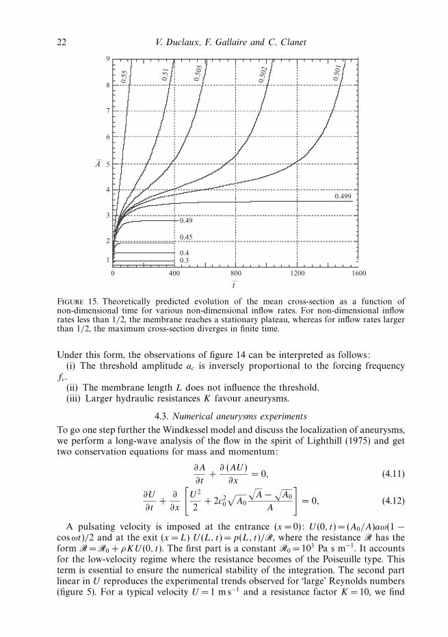
This analysis is confirmed by the numerical integration of (4.9) performed infigure 15 for different values of Qin. The two different behaviours (steady andaneurysm) are recovered and we also notice the similarity in the time evolution of thecross-section with the one measured experimentally (figure 13a).
A quantitative comparison of the non-dimensional threshold Qc = 1/2 is providedin figure 16, with a remarkable agreement regarding the exact prefactor if one bearsin mind the extreme simplicity of the Windkessel model considered here. Despite thetwo main limitations of the model, the time-averaging procedure resulting from theseparation of scales and the global character of the model, which fully neglectsthe inhomogeneities described in § 3, the agreement is excellent.
With dimensions, the critical mean flow Qc = 1/2 above which aneurysms areexpected is
Qc = A0acωc =A0c0√
2K. (4.10)
22 V. Duclaux, F. Gallaire and C. Clanet
0
1
2
3
4
5
6
7
8
9
A–
t–400
0.30.4
0.45
0.49
0.499
0.50
1
0.50
2
0.50
5
0.51
0.55
800 1200 1600
Figure 15. Theoretically predicted evolution of the mean cross-section as a function ofnon-dimensional time for various non-dimensional inflow rates. For non-dimensional inflowrates less than 1/2, the membrane reaches a stationary plateau, whereas for inflow rates largerthan 1/2, the maximum cross-section diverges in finite time.
Under this form, the observations of figure 14 can be interpreted as follows:(i) The threshold amplitude ac is inversely proportional to the forcing frequency
fc.(ii) The membrane length L does not influence the threshold.(iii) Larger hydraulic resistances K favour aneurysms.
4.3. Numerical aneurysms experiments
To go one step further the Windkessel model and discuss the localization of aneurysms,we perform a long-wave analysis of the flow in the spirit of Lighthill (1975) and gettwo conservation equations for mass and momentum:
∂A
∂t+
∂ (AU )
∂x= 0, (4.11)
∂U
∂t+
∂
∂x
[U 2
2+ 2c2
0
√A0
√A −
√A0
A
]= 0, (4.12)
A pulsating velocity is imposed at the entrance (x =0): U (0, t) = (A0/A)aω(1 −cosωt)/2 and at the exit (x = L) U (L, t) =p(L, t)/R, where the resistance R has theform R = R0 + ρKU (0, t). The first part is a constant R0 = 103 Pa s m−1. It accountsfor the low-velocity regime where the resistance becomes of the Poiseuille type. Thisterm is essential to ensure the numerical stability of the integration. The second partlinear in U reproduces the experimental trends observed for ‘large’ Reynolds numbers(figure 5). For a typical velocity U = 1 m s−1 and a resistance factor K = 10, we find

A fluid mechanical view on abdominal aortic aneurysms 23
2 4 6 8 10 12 14
(f c
LK
/2)/
c 0
L/2ac
0
0.5
1.0
1.5
Figure 16. Non-dimensional critical frequency at the onset of an aneurysmfc = ((L
√K/2)/c0)fc as a function of 1/2ac , half the inverse of the non-dimensional critical
amplitude ac = ac/L for the aneurysms reported in figure 14. The predicted linear dependencewith slope 1/2π is shown by the solid line.
that the second component of the resistance is 10 times larger than the constant R0.The numerical resistance is thus close to that observed experimentally.
Equations (4.11) and (4.12) are solved using a finite-difference Lax–Friedrich scheme(see the Appendix) and a constant ratio U/(dx/dt) = 1/2 satisfying the Courant–Friedrichs–Lewy (CFL) condition. In this expression, dx and dt represent the spaceand time discretization intervals, respectively. As discussed by Hirsch (1989), this CFLcondition is a necessary condition for convergence of the numerical integration.
In order to mimic the formation of aneurysms with our numerical model, we haveobserved that is was compulsory to introduce a more elastic region of the membrane,as shown in figure 17, so as to prevent numerical instabilities at the outlet boundarycondition. In the following, we have used a defect of width δ = L/4 (figure 17)and wave speed c1 = c0/
√2, located in the middle of the membrane. Note that the
intensity of this defect could have been kept very low at the expense of a reducedtime step. This in turn would have increased artificially the numerical dissipation ofthe Lax–Friedrich scheme and spuriously damped the dynamics.
Typical results are shown in figure 18 for a numerical membrane with K = 60,L = 4 m, f = 1 Hz and c2
0 = 35 m2 s−2. As in the experiment, two regimes areeasily identified. For amplitudes less than 252 mm, the membrane reaches amean stationary plateau of the cross-section A∞ whereas for amplitudes largerthan 252 mm, the maximum diameter diverges in finite time. Again, beyond thethreshold, a characteristic settling time teq of a few dozen of cardiac cycles may beidentified.

24 V. Duclaux, F. Gallaire and C. Clanet
C02(x)
xd
R(x,t)
δ
∆
Figure 17. Typical inhomogeneous membrane properties used in the numerical experiments.
2.0(×10–3)
a = 360 mm a = 270 mm
a = 243 mm
1.8
1.6
1.4
1.2
Am
ax (m
2 )
1.0
0.8
0.6
0.4
0.2
0 10 20 30 40
t50 60 70 80
a = 216 mm
a = 162 mm
a = 90 mm
a = 234 mm
Figure 18. Evolution of the maximum cross-section as a function of time for various pistonamplitudes a; K = 60, L =4 m, f = 1 Hz, c2
0 = 35 m2 s−2. For amplitudes less than 252 mm,the membrane reaches a stationary plateau once the oscillations based on the cardiac cycleare filtered, whereas for amplitudes larger than 252 mm, the maximum cross-section divergesin finite time.
The numerical calculations are complementary to the experimental measurements,since they enable one to easily vary L and K . A comparison of the threshold forunbounded growth obtained in the numerical model and the experiment is providedin figure 19 in the non-dimensional 1/2ac–fc plane. Here, fc = fcL
√K/2/c0 and
ac = ac/L, in accordance with the previous section. The linear relationship, predictedby the nonlinear Windkessel model, is again verified here and it shows that aneurysmsare formed whenever the flow rate Q =A0aω becomes larger than Qc ∼ A0c0/
√2K .
There is however a discrepancy in the proportionality factor between the experimentand the numerical model. Several plausible interpretations may be proposed. Thetemporal flow rate signal in the numerical experiments differs from the experimentallyimposed flow rate. Whereas a sinusoidal signal is used in the numerical integration,the experimental signal is more like a truncated sinus wave. It is likely that for a givenamplitude and frequency, the peak experimental influx is larger than the numericalinflux. Another difference lies in the fact that the membrane used in the numericalmodel does contain a localized defect.

A fluid mechanical view on abdominal aortic aneurysms 25
20
18
16
14
12
10f–c
8
6
4
2
0 5 10 15 20 25
1/2a–c
30 35 40 45 50
Figure 19. Non-dimensional threshold amplitude and frequency (denoted by open circles)for aneurysm in the numerical model (integration of the system (4.11) and (4.12)) for variouslengths L and hydraulic resistances K; the dashed line refers to the predicted linear dependencewith slope 1/2π (4.10).
4.4. Influence of the nonhomogeneous deformations of the membraneonto the aneurysm threshold
Section 3 was devoted to the analysis of various regimes of deformation of themembrane below the aneurysm threshold. It was shown that if the forcing timebecomes smaller than the Windkessel settling time, the membrane could not fill andempty as a whole and becomes non-homogeneous. In the present section, we aimat considering the effect of such inhomogeneities onto the formation of aneurysmand to answer the question if they are particular regions in the membrane whichencounter aneurysm at first as a consequence of focalization. From an experimentalpoint of view, we have always observed aneurysms forming close to the end of themembrane, but we should remember that the length of the membrane could not bemuch varied, preventing a more systematic analysis. The numerical model should inprinciple enable a detailed study, but unfortunately it is not appropriate to yield adirect answer. Indeed, it is not possible to use a uniform membrane since in that caseaneurysms would form at the end point and destabilize the boundary condition.
It is however possible to study the influence of the forcing-induced inhomogeneitiesin an indirect manner. For a given membrane, the position xd and the amplitude∆ =(c2
0 − c2min)/c
20 of the defect (see figure 17) can be varied until the aneurysm is
triggered. Such a numerical experiment is shown in figure 20.Figure 20(a1) shows that for the same defect intensity and width, the position of the
centre of the defect has an influence on the aneurysm threshold. Indeed, for a defectlocated in the middle of the membrane xd =L/2, an aneurysm is formed, whereas fordefects located upstream or downstream, the membrane reaches a mean equilibriumaveraged shape shown in figure 20(a2). This time-averaged mean shape displays abulge at the position of the defect, since the membrane is locally more distensible. Thecorresponding shape for xd =L/2 is not plotted since an aneurysm takes place, but forlower values of the defect intensity, the resulting bulge surpasses (not shown) thoseobtained for xd = L/3 and xd = 2L/3, and one may infer that, prior to aneurysm, the

26 V. Duclaux, F. Gallaire and C. Clanet
2.2
(a)
(b) (d )
(c)A
(m
2 )A
(m
2 )2.00
0.16
0.12
0.08
0.04
2.0
1.8
1.6
1.4
1.2
1.0
0.8
0.6
0.4
1.6
L /3
(×10–3)
(×10–3) (×10–3)2L /3
1.4
1.2
1.0
0.8
0.6
0.4
0.2
1.6
1.4
1.2
1.0
0.8
0.6
0.4
0.2
0
0 0.4 0.8 1.4 1.6 2.0 0 0.4 0.8 1.4
minmin
moymoy
max
max
1.6 2.0
0 0.4 0.8 1.2 1.6 2.010 20
t (s)x
xx
30 40
x = 2L/3
x = L/3
x = L/2
∆*
Figure 20. Numerical experiments on the influence of the position of the defect for amembrane with L = 2 m, f = 1 Hz, a = 360 mm, K = 200. (a) Time evolution of the maximalcross-section along the membrane, for three different positions of the same defect (∆ = 0.12).(b) Maximal (max), minimal (min) and time-averaged (moy) mean cross-sections foran homogeneous membrane (∆=0), and the two imperfect membranes at equilibrium:xd = L/3,∆ = 0.12 and xd = 2L/3,∆ = 0.12. (c) Threshold value of ∆∗ required for thetriggering of an aneurysm as a function of the position of the defect. The hashed zonecould not be reached for numerical stability reasons. (d ) Maximal, minimal and time-averagedmean cross-sections for an homogeneous membrane (∆=0), displaying highs and lows. Thelowest ∆∗ is obtained in the crest whereas the highest ∆∗ is obtained in the trough.
maximum deformation with a localized defect increases with the mean deformationof the reference perfect membrane at the position of the defect. The influence ofthe defect location on the threshold for aneurysm is investigated quantitatively infigure 20(b1,b2), where the lowest required defect intensity is obtained for the positionof the maximum focalization in the membrane without defect. Conversely, locationswhere the focalization is not active correspond to high threshold defect intensities. Inthis figure, positions of the defect close to the ends of the membrane could not beexplored for numerical instability reasons.

A fluid mechanical view on abdominal aortic aneurysms 27
0.2
(a)
(b)
0.1
1.5
1.0
0.5
0.20 0.4x
0.6 0.8 1.0
0
(×10–3)
A (
m2 )
∆*
Figure 21. Numerical experiments on the influence of the position of the defect, similar tofigure 20(b), with L =1 m, f = 1 Hz, a = 360 mm, K = 200.
A similar analysis with the same trends is provided in figure 21 for anothermembrane length L. The lowest required defect intensity ∆∗ is observed at thelocation of the reference membrane crests whereas the highest ∆∗ is obtained inthe trough. This confirms the influence of focalization onto the threshold for theformation of an aneurysm.
4.5. Physiological implications
Using formula (4.10) with a suitable prefactor to fit the experimental data andparameters suited to the aorta, A0 = 3 × 10⁻⁴ m2, c0 = 5 m s−1, K = 10, the thresholdinflow becomes Qc = 50 ml s−1. This value is lower than the cardiac flux 80 ml cycle−1,but note that only 50–70 % of the flux goes into the aorta, the remaining flowing intothe coronary and carotid arteries so that the order of magnitude of our threshold isclose to the typical aortic blood flow rate.
Let us now discuss the possible link between our simple scaling law on the criticalflow rate and the well-accepted risk factors for aneurysms:
(a) the age of the patient, inducing a rigidification of the aorta and other largearteries;
(b) hypertension, also associated with the rigidification of the aorta andaugmentation of the mean and peak systolic pressure;
(c) atherosclerosis, i.e. the local deposition of lipidic calcified constituents leadingto a stenosis;
(d) Marfan syndrome, a congenital disease that leads to a reduced elastin in thearteries wall.
28 V. Duclaux, F. Gallaire and C. Clanet
Regarding risk factors (a) and (b), the rigidification of iliac arteries leads to anincreasing K , favouring aneursyms. The rigidification of the aorta however also leadsto an increasing c0, which should at first glance help to avoid aneurysms. However,the increased mean pressure produced by the heart to drive the flow through the morerigid membrane is associated with an increase in the peak diastolic pressure. Thispoint needs to be explored in a subsequent study. Atherosclerosis (c) may lead to astenosis in the illiac increasing K . Alternatively, if the stenosis takes place in the aorta,the induced recirculation in the wake of the stenosis may lead to an enhancement ofthe shear in this lee region (Lasheras 2007), locally altering the mechanical propertiesof the aorta wall and ultimately weakening the elasticity properties in a finite region(Ku et al. 1997). As shown in the preceding subsection, this weakened region isan excellent candidate for aneurysm formation. Finally, in the presence of Marfansyndrome (d ), the reduced elastin fraction leads to a lower c0 that favours aneurysmformation.
4.6. Further comments on the relevance of the study
Note that the criterion (4.10) for aneurysm formation is based on the existence ofa local maximum in the pressure law P (R). In this paragraph, we refer to generalfeatures of membrane stability and use them to discuss the relevance of our resultswith respect to real aneurysms.
For a cylindrical membrane characterized by a pressure law P (R) and filled with aliquid which moves from high- to low-pressure regions, it is straight forward to showthat stable cylinders correspond to dP/dR > 0 while membranes such that dP/dR < 0are unstable. A consequence of this remark is that capillary jets for which P (R) = γ /R
(γ > 0 represents the surface tension) are always unstable since dP/dR = −γ /R2.This conclusion is correct in the long wavelength limit and is known as the Savart–Plateau–Rayleigh instability (Savart 1833; Plateau 1849; Rayleigh 1879).
For an elastic membrane law such as (2.2), one finds dP/dR =Ed0/R20[(2 −
R/R0)/(R/R0)]. The membrane is thus expected to be stable in the range R/R0 < 2and to turn unstable above this critical value, as shown in § 4. More generally, theexistence of this stable to unstable transition is associated with the existence of amaximum in the P (R) curve.
Now, let us show that the existence and typical geometry of aneurysms imposesthe existence of such a maximum: since an aneurysm is a dilatation of a cylindricalartery which develops over the years, it does not evolve significantly on the time scaleτ of few hundreds of heart beat cycles, and on this time scale, we can thus thinkof it as a steady deformation of the artery. Associating a mean pressure p with themean flow, one can see that two states of different radii coexist in the membraneat the same mean pressure, similar to the case of an elastic membrane shown infigure 22(b). These two states E1 and E2 are reported in the general pressure–radiusdiagram in figure 22(a). These two states of different radii are stable on the timescale τ which imposes that dP/dR is positive in E1 and E2. The segments [AB]and [CD] have thus positive slopes. Assuming that P (R) is continuous, i.e. a slowlyvarying (in space and time) membrane law can be used, one deduces that the portion[BC] will necessary contain a region of the negative slope. This shows the existenceof a maximum between E1 and E2 which is at the origin of the shape instabilitywhich has led from the initial straight cylinder to the bulgy one.
For such an elastic membrane as we have used, this maximum originates directlyin the cylindrical geometry and can be treated as a mechanical analogue of coexistentphases and treated with a Maxwell rule (Chater & Hutchinson 1984a,b). For a real

A fluid mechanical view on abdominal aortic aneurysms 29
P(R
)
p–
R1 R2 R
A
B D
C
R2R1
(a)
(b)
E1 E2
Figure 22. (Colour online) (a) General picture for the pressure–radius relation P (R) on amembrane which presents a stationary dilatation (b).
artery, the maximum has probably a different origin, resulting from the competitionof geometrical and elastic nonlinearities. Still, as stressed above, the existence ofaneurysms indicates that it should exist.
5. ConclusionAbdominal aortic aneurysms are a dilatation of the aorta localized preferentially
close to the bifurcation of the iliac arteries and which increases in time. Understandingtheir localization and growth rate remain two open questions which can havebiological or physical origin or both. In order to identify the respective roles ofthe biological and physical processes, we have addressed these two questions ofthe localization and growth using a simplified physical experiment consisting of thepulsating flow in an elastic membrane in similarity with the flow in a human aorta.
We first show that submitted to an oscillating flow, the elastic membrane canundergo either an homogeneous deformation or an inhomogeneous deformation. Weshow that the transition between these two types of deformations is sensitive to boththe frequency and the amplitude of the forcing. We propose a scaling argument tounderstand this transition and suggest a connection with the localization of realaneurysms.
Concerning the formation and development of bulges along the elastic membrane,we propose a simple model that captures the physics of the shape transition: in ourelastic membrane, an ‘aneurysm’ forms whenever the time-averaged inflow is highenough for the time-averaged diameter of the membrane to double from its basevalue. At this specific dilatation, the relation between the inner pressure and thediameter presents a maximum, a property needed to observe the instability.

30 V. Duclaux, F. Gallaire and C. Clanet
The modifications brought to this global view by the influence of the localinhomogeneities in space has been tentatively discussed with the numerics and it isshown that the places where bulges develop are strongly related to the inhomogeneityof the deformation.
While discussing the possible application of this simple model to real aneurysms,we show that the critical flow rate criterion is compatible with most of known riskfactors.
At this point, we have to underline that even if this simple model is promising,important biological factors such as the remodelling of the membrane properties havenot been considered, and must be included in future work.
Similarly, we underline that in our experiments the time-dependent flow rate isprescribed, independent of the state of the latex tube or the downstream resistance.However, the heart does not exactly behave as a pure flow source, and if the peripheralresistance is changed, both the pressure and the flow pulses also change. This feedbackloop will also be an interesting complement to the present model.
We thank B. Levy and A. Tedgui from INSERM U 541, Hopital Lariboisiereas well as P. Boutouyrie Inserm – U652 HEGP for the time they have allowed todiscussions on the appropriate way to model aneurysms in a physics laboratory.
Appendix. Detailed numerical schemeEquations (4.11) and (4.12) are discretized on a uniform finite difference grid with
spacing dx according to
Ap+1n =
Ap
n−1 + Ap
n+1
2+
dt
2dx
(U
p
n+1Ap
n+1 − Up
n−1Ap
n−1
), (A 1)
Up+1n =
Up
n−1 + Up
n+1
2+
dt
2dx
⎛⎝(
Up
n+1
)2
2+ c2
n+12√
πR0
√A
p
n+1 −√
A0
Ap
n+1
−(U
p
n−1
)2
2· · · − c2
n−12√
πR0
√A
p
n−1 −√
A0
Ap
n−1
), (A 2)
where n refers to the spatial index, p refers to the temporal index and dt is the timediscretization interval. Note that in these equations c0 has been replaced by c(x), afunction of x, which enables us to consider the membrane with non-uniform elasticity.The limit conditions used at the entrance are
Ap+11 = A
p
1 +dt
dx
(U
p
2 Ap
2 − Up
1 Ap
1
), (A 3)
Up+11 =
Dp+1
Ap
1
, (A 4)
where Dp+1 = D(0, t = (p + 1)δt) = A0aω (−1 + cos[ω(p + 1)δt]) /2. At the exit weimpose
Ap+1N = A
pN +
dt
dx
(U
pNA
pN − U
p
N−1Ap
N−1
), (A 5)
Up+1N = −2ρc2
N
√πR0
√A
pN −
√A0
RApN
, (A 6)
with R = R0 + ρKU (0, t).

A fluid mechanical view on abdominal aortic aneurysms 31
REFERENCES
Alexander, J. J. 2004 The pathobiology of aortic aneurysms. J. Surg. Res. 117, 163–175.
Carpenter, P. W. & Pedley, T. J. 2003 Flow in Collapsible Tubes and Past Other Highly ComplaintBoundaries. Kluwer.
Chandran, K. B. & Yearwood, T. L. 1981 Experimental study of physiological pulsatile flow in acurved tube. J. Fluid Mech. 111, 59–85.
Chater, E. & Hutchinson, J. W. 1984a On the propagation of bulges and buckles. J. Appl. Mech.51, 269–277.
Chater, E. & Hutchinson, J. W. 1984b Mechanical analogs of coexistent phases. In PhaseTransformations and Material Instabilities in Solids, pp. 21–36. Academic Press Inc. ISBN0-12-309770-3.
de Chauliac, G. 1373 La grande chirurgie (ed. C. Michel). Imprimeur de l’Universite de Montpellier.
Cheng, C. P., Herfkens, R. J. & Taylor, C. A. 2003 Abdominal aortic hemodynamic conditionsin healthy subjects aged 50–70 at rest and during lower limb exercise: in vivo quantificationusing MRI. Atherosclerosis 168, 323–331.
Frank, O. 1905 Der Puls in den Arterien. Z. Biol. 45, 441–553.
Fung, Y. C. 1990 Biomechanics: Motion, Flow, Stress and Growth. Springer.
Fung, Y. C. 1997 Biomechanics: Circulation. Springer.
Gray, H. 1918 Anatomy of the Human Body. Lea and Febiger.
Glagov, S., Rowley, D. A. & Kohut, R. 1961 Atherosclerosis of human aorta and its coronaryand renal arteries. Arch. Pathol. Lab. Med. 72, 558–568.
Groenink, M., Langevaka, S. E., Vanbavel, Ed., van der Wall, E. E., Mulder, B. J. M., van der
Wal, A. C. & Spaan, J. A. E. 1999 The influence of aging and aortic stiffness on permanentdilation and breaking stress of the thoracic descending aorta. Cardiovasc. Res. 43, 471–480.
Guirguis, E. M. & Barber, G. G. 1991 The natural history of abdominal aortic aneurysms. Am.J. Surg. 162, 481–483.
Hirsch, C. 1989 Numerical Computation of Internal and External Flows. Wiley.
Humphrey, J. D. & Delange, S. L. 2004 An Introduction to Biomechanics (Solids and Fluids, Analysisand Design). Springer.
Ku, D. N. 1997 Blood flow in arteries. Annu. Rev. Fluid Mech. 29, 399–434.
Ku, D. N., Zeigler, M. N. & Downing, J. M. 1990 One-dimensional steady inviscid flow througha stenotic collapsible tube. J. Biomech. Engng 112, 444–450.
Laennec, R. T. H. 1819 De l’auscultation Mediate ou Traite du Diagnostic des Maladies des Poumonset du Coeur, Fonde Principalement Sur ce Nouveau Moyen d’exploitation. J. A. Brosson &J. S. Chaud.
Lasheras, J. C. 2007 The biomechanics of arterial aneurysms. Annu. Rev. Fluid Mech. 39, 293–319.
Li, J. K., Malbin, J., Riffle, R. A. & Noodergraaf, A. 1981 Pulse wave propagation. Circ. Res.49, 442–452.
Lighthill, J. 1975 Mathematical Biofluiddynamics. SIAM.
McAuley, L. M., Fisher, A., Hill, A. B. & Joyce, J. 2002 Les Implants EndovasculairesComparativement a la Chirurgie Sanglante Dans la Reparation de L’anevrisme de L’aorteAbdominale: Pratique au Canada et Examen Systematique. Rapport Technologique no. 33.Office canadien de coordination de l’evaluation des technologies de la sante.
McDonald, D. A. 1960 Blood Flow in Arteries. Edward Arnold.
McDonald, D. A. 1968 Regional pulse-wave velocity in the arterial tree. J. Appl. Physiol. 24, 73–78.
Medynsky, A. O., Holdsworth, D. W., Sherebrin, M. H., Rankin, R. N. & Roach, M. R. 1998Elastic response of human iliac arteries in-vitro to balloon angioplasty using high-resolutionCT1. J. Biomech. 31, 747–751.
Olsen, J. H. & Shapiro, A. H. 1967 Large amplitude unsteady flow in liquid-filled elastic tubes.J. Fluid Mech. 29, 513–538.
Paıdoussis, M. P. 2006 Wave propagation in physiological collapsible tubes and a proposal for aShapiro number. J. Fluids Struct. 22, 721–725.
Paquerot, J. F. & Lambrakos, S. G. 1994 Monovariable representation of blood flow in a largeelastic artery. Phys. Rev. E 49, 3432–3439.
Pedley, T. J. 1980 The Fluid Mechanics of Large Blood Vessels. Cambridge University Press.
32 V. Duclaux, F. Gallaire and C. Clanet
Plateau, J. A. F. 1849 Statique experimentale et theorique des liquides soumis aux seules forcesmoleculaires. Acad. Sci. Brux. Mem. 23, 5.
Prandtl, L. & Tietjens, O. G. 1957 Applied Hydro and Aeromechanics. Dover.
Rayleigh, Lord. 1879 On the instability of jets. Proc. Lond. Math. Soc. 10, 4–13.
Reinke, W., Johnson, P. C. & Gaehtgens, P. 1986 Effect of shear rate variation on apparentviscosity of human blood in tubes of 29 to 94 microns diameter. Circ. Res. 59, 124–132.
Roberts, J. C., Moses, C. & Wilkins, R. H. 1847 Autopsy studies in atherosclerosis: distributionand severity of atherosclerosis in patients dying without any morphologic evidence ofatherosclerotic catastrophe. Circulation 20, 511–519.
Savart, F. 1833 Memoire sur la constitution des veines liquides lancees par des orifices circulairesen mince paroi. Ann. de Chim. 53, 337–386.
Shapiro, A. H. 1977 Steady flow in collapsible tubes. ASME J. Biomech. Engng 99, 126–147.
Womersley, J. R. 1957 Oscillatory flow in arteries: the constrained elastic tube as a model ofarterial flow and pulse transmission. Phys. Med. Biol. 2, 178–187.