a fourth-order accurate finite-volume method with structured

SIAM J. SCI. COMPUT. c© 2012 Society for Industrial and Applied MathematicsVol. 34, No. 2, pp. B179–B201

A FOURTH-ORDER ACCURATE FINITE-VOLUME METHOD WITHSTRUCTURED ADAPTIVE MESH REFINEMENT FOR SOLVING

THE ADVECTION-DIFFUSION EQUATION∗

QINGHAI ZHANG† , HANS JOHANSEN‡ , AND PHILLIP COLELLA‡

Abstract. We present a fourth-order accurate algorithm for solving Poisson’s equation, the heatequation, and the advection-diffusion equation on a hierarchy of block-structured, adaptively refinedgrids. For spatial discretization, finite-volume stencils are derived for the divergence operator andLaplacian operator in the context of structured adaptive mesh refinement and a variety of boundaryconditions; the resulting linear system is solved with a multigrid algorithm. For time integration, wecouple the elliptic solver to a fourth-order accurate Runge–Kutta method, introduced by Kennedyand Carpenter [Appl. Numer. Math., 44 (2003), pp. 139–181], which enables us to treat the nonstiffadvection term explicitly and the stiff diffusion term implicitly. We demonstrate the spatial andtemporal accuracy by comparing results with analytical solutions. Because of the general formulationof the approach, the algorithm is easily extensible to more complex physical systems.

Key words. Poisson’s equation, the heat equation, the advection-diffusion equation, adaptivemesh refinement, additive Runge–Kutta method, finite volume, conservation form

AMS subject classifications. 76R99, 65M08, 65L06

DOI. 10.1137/110820105

1. Introduction. The advection-diffusion equation governs numerous physicalprocesses. Morton [17] lists ten sample applications ranging from semiconductor sim-ulation to financial modelling. He also observes that “Accurate modelling of theinteraction between convective and diffusive processes is the most ubiquitous andchallenging task in the numerical approximation of partial differential equations.”This observation is partly due to the fact that algorithms and analysis tend to bevery different in the two limiting cases of elliptic and hyperbolic equations. Also,even for very simple initial and boundary conditions, the true solution may containmultiple length-scales that vary drastically across the spatial domain; see (3.1) in [18]for such an example.

A finite-volume (FV) formulation is often preferred for applications where con-servation is a primary concern. In its simplest form, the FV formulation is derivedby applying the divergence theorem over the cells of a regular computational grid:

(1.1)1

hD

∫Vi

∇ · �Fdx =1

h

D∑d=1

(〈Fd〉i+ 1

2ed − 〈Fd〉i− 1

2ed

),

where a face-averaged quantity is defined as

(1.2) 〈Fd〉i+ 12e

d ≡ 1

hD−1

∫A

i+12ed

Fd dA.

∗Submitted to the journal’s Computational Methods in Science and Engineering section January5, 2011; accepted for publication (in revised form) January 17, 2012; published electronically April12, 2012.

http://www.siam.org/journals/sisc/34-2/82010.html†Applied Numerical Algorithms Group, High Performance Computing Research Department,

Lawrence Berkeley National Laboratory, Berkeley, CA 94720, and Department of Mathematics, Uni-versity of California, Davis, CA 95616 ([email protected]).

‡Applied Numerical Algorithms Group, High Performance Computing Research Department,Lawrence Berkeley National Laboratory, Berkeley, CA 94720 ([email protected], [email protected]).

B179

B180 QINGHAI ZHANG, HANS JOHANSEN, AND PHILLIP COLELLA

Here h denotes the uniform mesh spacing, i ∈ ZD a cell multi-index, and ed ∈ Z

D

the vector with its dth component equal to one and all other components zero. Let1l ∈ Z

D be the vector whose elements are all equal to one; then Vi = [ih, (i + 1l)h]denotes a grid cell, and Ai− 1

2ed = [ih, (i+1l− ed)h] and Ai+ 1

2ed = [(i+ ed)h, (i+1l)h]

denote the two faces of cell Vi along the dth dimension.The relationship (1.1) is exact; approximations are obtained from replacing the

integrals over faces (1.2) by quadratures. Traditionally, FV methods have been basedon using the midpoint rule for the face integrals, which leads to a second-order accu-rate discretization. More recently, there has been increasing interest in using methodsbased on higher-order accurate FV methods of this form, with quadratures using themidpoint rule plus corrections computed using the transverse derivatives of the fluxes,or, for the case of fluxes that are linear functions of the unknowns, using deconvolutionof face-averages from cell averages, following the ideas in [8, 21]. This has been donefor Poisson’s equation [1], for hyperbolic problems on mapped grids [7], and for non-linear hyperbolic conservation laws on locally refined grids [14]. For time-dependentproblems, a method-of-lines approach has been employed, using the high-order dis-cretization methods in space and the classical explicit fourth-order accurate Runge–Kutta method in time. In this paper, we demonstrate that the approach describedabove can be used for advection-diffusion problems based on a semi-implicit timediscretization. In particular, we use a fourth-order accurate additive Runge–Kuttamethod described in [12], treating the advection terms explicitly and the diffusionterms implicitly, with the spatial discretization performed on locally refined grids.The resulting method is fourth-order accurate, with a time-step stability constraintrequired only for the explicitly treated advection term.

2. FV formulation. The advection-diffusion equation is defined as

(2.1)∂φ

∂t= −∇ · (uφ) + νΔφ+ f,

where the constant diffusivity ν, the velocity field u = u(x, t), and the forcing termf = f(x, t) are known a priori. To generate an FV discretization, we average (2.1)over each control volume, Vi, and apply the divergence theorem as in (1.1) to obtaina system of ordinary differential equations (ODEs) on Z

D:

(2.2a)d 〈φ〉idt

= Ladv(〈φ〉 , t)i + Ldiff(〈φ〉)i + 〈f〉i ,

(2.2b) Ladv(〈φ〉 , t)i = − 1

h

D∑d=1

(〈udφ〉i+ 1

2 ed − 〈udφ〉i− 1

2ed

),

(2.2c) Ldiff(〈φ〉)i = ν 〈Δφ〉i =ν

h

D∑d=1

(⟨∂φ

∂xd

⟩i+ 1

2 ed

−⟨∂φ

∂xd

⟩i− 1

2ed

),

where a cell-averaged quantity is defined as

(2.3) 〈q〉i ≡1

hD

∫Vi

q(x, t)dx.

Note that (2.2a)–(2.2c) are still exact relationships with no discretization error.

FOURTH-ORDER AMR FOR ADVECTION-DIFFUSION EQUATION B181

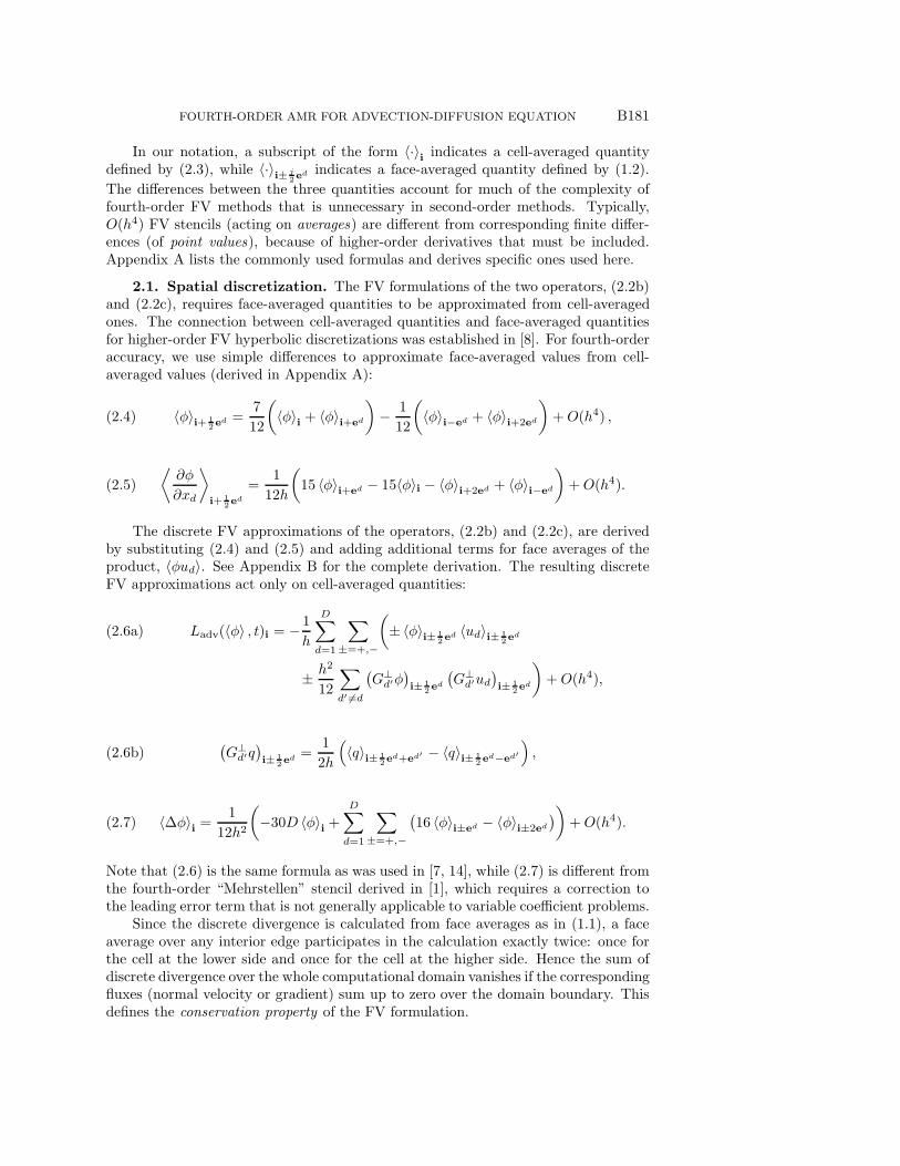
In our notation, a subscript of the form 〈·〉i indicates a cell-averaged quantitydefined by (2.3), while 〈·〉i± j

2ed indicates a face-averaged quantity defined by (1.2).

The differences between the three quantities account for much of the complexity offourth-order FV methods that is unnecessary in second-order methods. Typically,O(h4) FV stencils (acting on averages) are different from corresponding finite differ-ences (of point values), because of higher-order derivatives that must be included.Appendix A lists the commonly used formulas and derives specific ones used here.

2.1. Spatial discretization. The FV formulations of the two operators, (2.2b)and (2.2c), requires face-averaged quantities to be approximated from cell-averagedones. The connection between cell-averaged quantities and face-averaged quantitiesfor higher-order FV hyperbolic discretizations was established in [8]. For fourth-orderaccuracy, we use simple differences to approximate face-averaged values from cell-averaged values (derived in Appendix A):

(2.4) 〈φ〉i+ 12e

d =7

12

(〈φ〉i + 〈φ〉i+ed

)− 1

12

(〈φ〉i−ed + 〈φ〉i+2ed

)+O(h4) ,

(2.5)

⟨∂φ

∂xd

⟩i+ 1

2ed

=1

12h

(15 〈φ〉i+ed − 15〈φ〉i − 〈φ〉i+2ed + 〈φ〉i−ed

)+O(h4).

The discrete FV approximations of the operators, (2.2b) and (2.2c), are derivedby substituting (2.4) and (2.5) and adding additional terms for face averages of theproduct, 〈φud〉. See Appendix B for the complete derivation. The resulting discreteFV approximations act only on cell-averaged quantities:

Ladv(〈φ〉 , t)i = − 1

h

D∑d=1

∑±=+,−

(±〈φ〉i± 1

2 ed 〈ud〉i± 1

2ed(2.6a)

± h2

12

∑d′ �=d

(G⊥

d′φ)i± 1

2 ed

(G⊥

d′ud)i± 1

2ed

)+O(h4),

(2.6b)(G⊥

d′q)i± 1

2 ed =

1

2h

(〈q〉i± 1

2ed+ed′ − 〈q〉i± 1

2 ed−ed′

),

(2.7) 〈Δφ〉i =1

12h2

(−30D 〈φ〉i +

D∑d=1

∑±=+,−

(16 〈φ〉i±ed − 〈φ〉i±2ed

))+O(h4).

Note that (2.6) is the same formula as was used in [7, 14], while (2.7) is different fromthe fourth-order “Mehrstellen” stencil derived in [1], which requires a correction tothe leading error term that is not generally applicable to variable coefficient problems.

Since the discrete divergence is calculated from face averages as in (1.1), a faceaverage over any interior edge participates in the calculation exactly twice: once forthe cell at the lower side and once for the cell at the higher side. Hence the sum ofdiscrete divergence over the whole computational domain vanishes if the correspondingfluxes (normal velocity or gradient) sum up to zero over the domain boundary. Thisdefines the conservation property of the FV formulation.


2.2. Boundary conditions. At nonperiodic domain boundaries, “ghost cells”are used with the standard interior stencils to evaluate the advection and Laplacianoperators. For example, let 〈φ〉i denote the cell-averaged scalar of the interior cellabutting a high-side boundary, and let 〈φ〉i+ed & 〈φ〉i+2ed denote those of the twoghost cells to be calculated. In the case of Dirichlet boundary conditions, we specify〈φ〉i+ 1

2ed = 〈g〉i+ 1

2 ed and use an extrapolation based on the integrals of interpolating

polynomials; this leads to the following ghost cell formulas for the fourth-order case:

(2.8a) 〈φ〉i+ed =1

3

(−13 〈φ〉i + 5 〈φ〉i−ed − 〈φ〉i−2ed + 12 〈g〉i+ 1

2ed

)+O(h4),

(2.8b) 〈φ〉i+2ed =1

3

(−70 〈φ〉i + 32 〈φ〉i−ed − 7 〈φ〉i−2ed + 48 〈g〉i+ 1

2ed

)+O(h4).

A fifth-order interpolation leads to(2.9a)

〈φ〉i+ed =1

12

(−77 〈φ〉i + 43 〈φ〉i−ed − 17 〈φ〉i−2ed + 3 〈φ〉i−3ed + 60 〈g〉i+ 1

2ed

)+O(h5)

〈φ〉i+2ed =1

12


2 ed

)(2.9b)

+O(h5).

Similarly, for Neumann-type boundary conditions we specify 〈 ∂φ∂xd

〉i+ 12 e

d = 〈g〉i+ 12 e

d ,

and a fourth-order interpolation yields

(2.10a) 〈φ〉i+ed =1

11

(9 〈φ〉i + 3 〈φ〉i−ed − 〈φ〉i−2ed + 12 〈g〉i+ 1

2 ed

)+O(h4),

(2.10b) 〈φ〉i+2ed =1

11

(−30 〈φ〉i + 56 〈φ〉i−ed − 15 〈φ〉i−2ed + 48 〈g〉i+ 1

2 ed

)+O(h4),

while a fifth-order interpolation yields(2.11a)

〈φ〉i+ed =1

10

(5 〈φ〉i + 9 〈φ〉i−ed − 5 〈φ〉i−2ed + 〈φ〉i−3ed + 12 〈g〉i+ 1

2ed

)+O(h5),

(2.11b)

〈φ〉i+2ed =1

10


2ed

)+O(h5).

We use fourth-order formulas (2.8) and (2.10) for the advection operator, and fifth-order formulas (2.9) and (2.11) for the Laplacian operator.

2.3. Nested refinement. The uniform grid discretization above can also beextended to structured adaptive mesh refinement (AMR), i.e., a locally refined, nestedhierarchy of rectangular grids. Our notation is based on previous O(h2) structuredAMR work (see [13]), but we will reiterate parts of the notation for the purpose ofexplaining the present algorithm.

On a family of nested discretizations of a rectangular domain {Γl}lmax

l=0 , Γl ⊂ ZD,

control volumes V li = [ihl, (i+1l)hl] are represented with multi-indices i ∈ Γl, with hl


denoting the uniform mesh spacing and nlref = hl−1/hl the refinement ratio between

levels Γl and Γl−1. To relate geometric regions and variables on different levels of thehierarchy to one another, we define a coarsening operator for indices,

Cnlref(i) =

(⌊i1

nlref

⌋, . . . ,

⌊iD

nlref

⌋).

Similarly, we define the refining operator as C−1nlref

(Γl−1) = Γl.

At any given point in time, our computed solution will be defined on the compu-tational domain {Ωl}lmax

l=0 , Ωl ⊂ Γl, Cnlref(Ωl) ⊂ Ωl−1, Ω0 = Γ0. The Ωl’s are assumed

to satisfy “proper nesting” conditions: that C−1nlref

(Cnlref(Ωl)) = Ωl (coarsening or refin-

ing levels does not change the region covered), and that there are at least sn pointsin any direction in Ωl separating Cnl+1

ref(Ωl+1) (the finer level coarsened to l) from

C−1nlref

(Ωl−1)− Ωl (the coarser level refined to l). In the case of periodic domains, this

condition is assumed to hold with respect to the periodic extensions of the grids. Inthe present work, we assume sn = 3 to support the interpolation stencils below.

The primary dependent variables on each level are defined only on the part of Ωl

not covered by finer grids:

(2.12a) φcomp = {φl}lmax

l=0 , φl : Ωlvalid → R,

(2.12b) Ωlvalid = Ωl − C−1

nl+1ref

(Ωl+1), Ωcomp =

lmax⋃l=0

Ωlvalid.

We generalize the definitions of the operators Ldiff, Ladv to operate on φcomp, butwith the flux calculations modified to account for the changes in grid resolution atrefinement boundaries. First, we extend the φl’s to all of Ωl by averaging down fromthe finer levels:

(2.13) 〈φ〉li =1

(nlref)

D

∑j∈C−1

nlref

({i})〈φ〉l+1

j on Cnl+1ref

(Ωl+1), l = lmax − 1, . . . , 0 .

Then, for each level, we compute approximate values of 〈φ〉 over control volumesoutside of Ωl to facilitate the evaluation of Ladv and Ldiff on all of Ωl

valid. Theconstrained least-squares approach described in [14] is adopted to derive these “coarse-fine” interpolation stencils.

Specifically, we interpolate O(hP+1)-order accurate values for j ∈ C−1nlref

({i}) by

computing a polynomial interpolant of the form

(2.14) Pi(x) =∑

p:pd≥0, p1+···+pD≤P

apxp, xp =

D∏d=1

xpd

d ,

subject to the constraint that the coarse 〈φ〉l are the averages of fine values 〈φ〉l+1j as

required by (2.13). The coefficients ap are computed as the least-squares approxima-tion to an overdetermined system of linear equations 〈φ〉j = 〈Pi〉j, j ∈ N (i), where

N (i) is a collection of nearby points in Ωl. The number of the chosen points ex-ceeds the number of terms in the sum in (2.14); the points must also be chosen so


〈F1〉2i− 12e1

〈F1〉2i+e2− 12e1

�� 〈F1〉i+ 12e1

〈F2〉i− 12e2

〈F2〉i+ 12e2

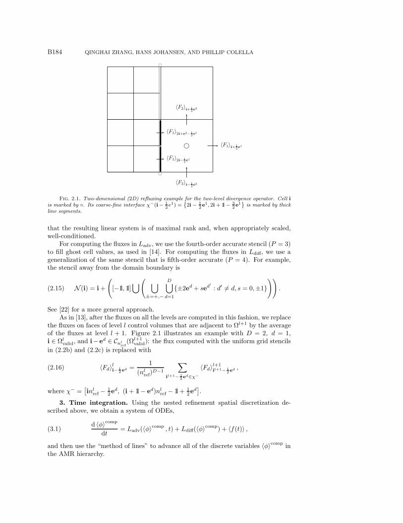
Fig. 2.1. Two-dimensional (2D) refluxing example for the two-level divergence operator. Cell iis marked by ◦. Its coarse-fine interface χ−(i− 1

2e1) =

{2i− 1

2e1, 2i+ 1l− 3

2e1

}is marked by thick

line segments.

that the resulting linear system is of maximal rank and, when appropriately scaled,well-conditioned.

For computing the fluxes in Ladv, we use the fourth-order accurate stencil (P = 3)to fill ghost cell values, as used in [14]. For computing the fluxes in Ldiff, we use ageneralization of the same stencil that is fifth-order accurate (P = 4). For example,the stencil away from the domain boundary is

(2.15) N (i) = i+

([−1l, 1l]

⋃( ⋃±=+,−

D⋃d=1

{±2ed + sed′: d′ = d, s = 0,±1}

)).

See [22] for a more general approach.As in [13], after the fluxes on all the levels are computed in this fashion, we replace

the fluxes on faces of level l control volumes that are adjacent to Ωl+1 by the averageof the fluxes at level l + 1. Figure 2.1 illustrates an example with D = 2, d = 1,i ∈ Ωl

valid, and i− ed ∈ Cnlref(Ωl+1

valid): the flux computed with the uniform grid stencils

in (2.2b) and (2.2c) is replaced with

(2.16) 〈Fd〉li− 12 e

d =1

(nlref)

D−1

∑il+1− 1

2 ed∈χ−

〈Fd〉l+1il+1− 1

2ed ,

where χ− =[inl

ref − 12e

d, (i + 1l− ed)nlref − 1l + 1

2ed].

3. Time integration. Using the nested refinement spatial discretization de-scribed above, we obtain a system of ODEs,

(3.1)d 〈φ〉comp

dt= Ladv(〈φ〉comp , t) + Ldiff(〈φ〉comp) + 〈f(t)〉 ,

and then use the “method of lines” to advance all of the discrete variables 〈φ〉comp inthe AMR hierarchy.


Our approach is to use an additive, implicit-explicit Runge–Kutta method in-troduced by Kennedy and Carpenter [12] for convection-diffusion-reaction equations.In particular, we select ARK4(3)6L[2]SA, a six-stage, fourth-order accurate, L-stablemethod, with an explicit treatment for the advection operator Ladv and source termf and an implicit treatment for the diffusion term Ldiff. Although this method hasbeen shown to suffer from the well-known problem of order reduction in the stiff limit[12, 15], it does have a good region of stability for the explicit terms, as shown in thenext section.

We integrate (3.1) by setting 〈φ〉(1) = 〈φ〉n, and then we calculate the five subse-

quent stage values 〈φ〉(s), s = 2, 3, 4, 5, 6, by solving

(3.2)(I −ΔtγLdiff

)〈φ〉comp,(s) = 〈φ〉n +ΔtL,

where

L =

s−1∑j=1

a[E]s,j

(Ladv

(〈φ〉comp,(j)

, t(j))+ 〈f〉 (t(j))

)+

s−1∑j=1

a[I]s,jLdiff

(〈φ〉comp,(j)

),

t(s) = tn+csΔt, and γ = a[I]s,s is a constant for all stages. The coefficients {a[E]

i,j }, {a[I]i,j},

{bj}, {cj} are defined in [12]; for completeness they are also provided in Appendix Cas decimal values [20].

At each intermediate stage s = 2, 3, 4, 5, 6, we must solve the Helmholtz-type lin-ear system (3.2), with its right-hand side explicitly calculated from values of previousstages. As discussed in [19, p. 441], the negation of the fourth-order discrete operator〈Δφ〉 defined in (2.7) is of essentially positive type [3], which carries the essential prop-erties of M-matrices such as positive definiteness. Consequently, the Helmholtz-typeoperator

(I − ΔtγLdiff

)also has eigenvalues of positive real parts; this can be veri-

fied by Fourier analysis. A standard multigrid method with Gauss–Seidel red-blackrelaxation [4] is employed in solving (3.2), with a V-cycle performed on each level ofthe AMR hierarchy. In the fourth-order case, writing the results of the red relaxationdirectly to the black points is incorrect, since the stencil as defined by (2.7) involvesboth red and black points. Instead we use an auxiliary storage to hold the results ofthe red relaxation in preparation for the ensuing black relaxation. As confirmed bythe numerical tests in section 5, this works well for both the Laplacian operator andthe Helmholtz-type operator.

Once all six stage values are known, the final calculation,

(3.3) 〈φ〉n+1 = 〈φ〉(6) +Δt6∑

j=1

(bj − a

[E]6,j

)(Ladv

(〈φ〉(j) , t(6)

)+ 〈f〉 (t(6))

),

provides the next time step value of 〈φ〉n+1, and the time integration procedure is

repeated.As the solution evolves in time, we allow the adaptive mesh grid hierarchy to

evolve as well. At the end of each time step, the grid hierarchy can be refined to trackemerging new features and/or coarsened to reduce computational expense. Typicallythe cells to be changed are “tagged” according to the evaluation of certain criteria;these criteria, specified by the user, are usually based on physical quantities or esti-mated errors. This dynamic grid generation is done in the standard fashion describedin [2, 13], by averaging down from finer grids to coarser grids as the former disappear,


and interpolating conservatively from coarser grids to newly refined regions. Theprincipal difference in the present AMR algorithm is the higher-order, conservativecoarse-fine interpolation and its supporting multigrid-based solver, as described aboveand in section 2.3.

4. Analysis. In this work, solution error refers to the difference between thetrue and the computed solutions. In contrast, truncation error relates to approximat-ing the advection and Laplacian operators, and it is caused by replacing continuousoperators with discrete finite-difference stencils in forming the ODE system (3.1).

4.1. Error analysis. Away from the coarse-fine interface and nonperiodic phys-ical domain boundaries, the truncation errors for these two operators are both O(h4);cf. (2.6) and (2.7). However, as discussed in the previous section, fourth- and fifth-order coarse-fine interpolations of the solution 〈φ〉 are used, respectively, for evalu-ating the advection and diffusion operators near the coarse-fine interface. Hence thetruncation error of both operators is O(h3) for control volumes near the coarse-fineinterface. A similar statement holds for a nonperiodic physical domain boundary, dueto the extrapolation formulas in section 2.2. These observations are consistent withthe discussion in Appendix B that the truncation error is O(h3) at the coarse-fineinterface due to refluxing. Nonetheless, we expect the 1-norm of the truncation errorto be O(h4), since the truncation error is O(h3) only on a set of codimension 1.

For Poisson’s equation, it is well known [10] that the accuracy of the solution errorwith respect to the ∞-norm is one order higher than that of the truncation error, solong as the lower-order truncation error is restricted to a set of codimension 1. Asfor diffusion processes with large higher-order derivatives and high Reynolds number(Re ≥ 105), the lower-order truncation errors on a set of codimension 1 might leadto solution errors of the same order [24, sect. 2]. However, since this work aims toaddress moderately stiff problems (with moderate to large ν), we expect the solutionerrors to be fourth-order accurate for all norm types.

4.2. Stability analysis. Using discrete Fourier analysis, we can convert theODE system (3.1), with constant velocity u and 〈f〉 = 0 on a periodic domain, to asystem of decoupled ODEs of the form

(4.1)dy

dt= λy =

(λd + iλa

)y,

where λd, iλa are the eigenvalues of the diffusion and advection operators:

(4.2a) λd = −4ν

h2

D∑d=1

sin2θd2

(1 +

1

3sin2

θd2

),

(4.2b) λa =|ud,max|

h

D∑d=1

sin θd

(1 +

2

3sin2

θd2

),

with θd ∈ (0, π). Note that in deriving (4.2) we have repeatedly applied the trigono-metric identities cos θ = 1− 2 sin2 θ

2 and sin θ = 2 sin θ2 cos

θ2 . The maximum value of

the scaled advection eigenvalue is then estimated as

(4.3) (λaΔt)max = CrD

(sin θ0 +

2

3sin θ0 sin

2 θ02

)max

≈ 1.37222DCr,


(a) overview (b) near the origin

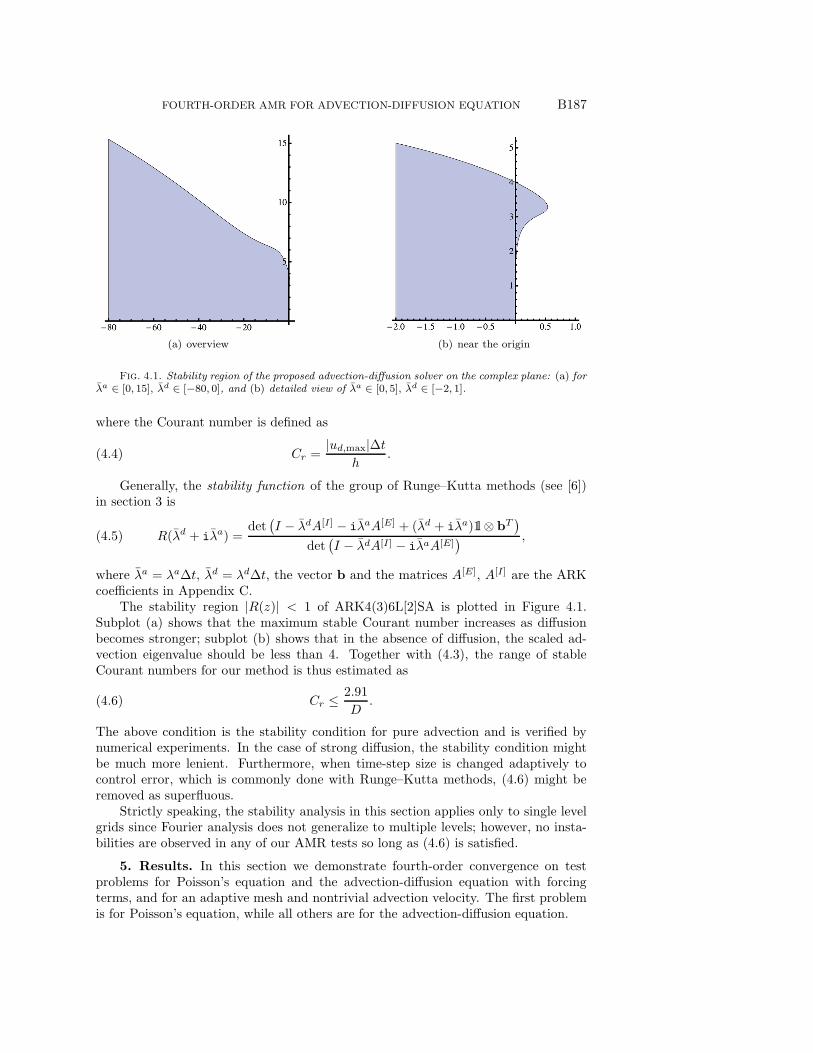
Fig. 4.1. Stability region of the proposed advection-diffusion solver on the complex plane: (a) forλa ∈ [0, 15], λd ∈ [−80, 0], and (b) detailed view of λa ∈ [0, 5], λd ∈ [−2, 1].

where the Courant number is defined as

(4.4) Cr =|ud,max|Δt

h.

Generally, the stability function of the group of Runge–Kutta methods (see [6])in section 3 is

(4.5) R(λd + iλa) =det

(I − λdA[I] − iλaA[E] + (λd + iλa)1l⊗ bT

)det

(I − λdA[I] − iλaA[E]

) ,

where λa = λaΔt, λd = λdΔt, the vector b and the matrices A[E], A[I] are the ARKcoefficients in Appendix C.

The stability region |R(z)| < 1 of ARK4(3)6L[2]SA is plotted in Figure 4.1.Subplot (a) shows that the maximum stable Courant number increases as diffusionbecomes stronger; subplot (b) shows that in the absence of diffusion, the scaled ad-vection eigenvalue should be less than 4. Together with (4.3), the range of stableCourant numbers for our method is thus estimated as

(4.6) Cr ≤ 2.91

D.

The above condition is the stability condition for pure advection and is verified bynumerical experiments. In the case of strong diffusion, the stability condition mightbe much more lenient. Furthermore, when time-step size is changed adaptively tocontrol error, which is commonly done with Runge–Kutta methods, (4.6) might beremoved as superfluous.

Strictly speaking, the stability analysis in this section applies only to single levelgrids since Fourier analysis does not generalize to multiple levels; however, no insta-bilities are observed in any of our AMR tests so long as (4.6) is satisfied.

5. Results. In this section we demonstrate fourth-order convergence on testproblems for Poisson’s equation and the advection-diffusion equation with forcingterms, and for an adaptive mesh and nontrivial advection velocity. The first problemis for Poisson’s equation, while all others are for the advection-diffusion equation.


Ω0

0 18

14

38

12

58

34

78

1

0

18

14

38

12

58

34

78

1

Ω10 Ω1

1

Ω12 Ω1

3 Ω14

Ω16Ω2

0

Fig. 5.1. A static locally refined grid hierarchy for Problem 1. The coarsest level (� = 0) coversthe problem domain [0, 1]D. The light gray area represents the intermediate level (� = 1), which isdecomposed by the dashed lines into seven rectangles, all of which range from 3/8 to 5/8 in the thirddimension. The finest level (� = 2), represented by the dark gray square, is obtained by shrinkingΩ1

5 to half of its length in each dimension.

5.1. Problem 1: Composite sinusoidal waves. We first address a test prob-lem similar to one in [1] for Poisson’s equation on the problem domain [0, 1]D withthe exact solution

(5.1) φ(x) =∑k

D∏d=1

sin(kπxd),

where {k} is a set of even integers representing different frequencies. Since the AMRLaplacian operator may depend on data from both coarser and finer levels, we use astatic, three-level grid layout with a refinement ratio of nref = 2, as shown in Figure5.1. The right-hand side of Poisson’s equation is initialized exactly by using an ana-lytical expression for 〈Δφ〉i derived from (5.1). The values of Dirichlet and Neumannboundary conditions in section 2.2 are calculated from sixth-order quadratures usingthe exact solution.

The truncation error and solution error are shown in Tables 5.1 and 5.2. Acrossdifferent types of boundary conditions, there are no differences in errors or convergencerates. As discussed in section 4.1, although the truncation error of Poisson’s equationis of third order, the solution can still be fourth-order accurate, even in the ∞-normsense. In addition, Figure 5.2 demonstrates satisfactory multigrid convergence, usingonly two relaxation pre- and postsweeps during the multigrid V-cycle across the locallyrefined grid hierarchy.

5.2. Problem 2: Traveling sinusoidal waves. For this test, we use an expres-sion of the form φ =

∏d sin(kdxd−udt) as an exact solution to the advection-diffusion


Table 5.1

Truncation and solution errors of the AMR elliptic solver applied to Problem 1 in two and threedimensions, with periodic boundary conditions and wave numbers {k} = {2, 4}. The static locallyrefined hierarchy is shown in Figure 5.1.

Base grid h 1/64 Rate 1/128 Rate 1/256 Rate 1/512

2D truncation L∞ 3.57e-01 2.97 4.56e-02 2.99 5.73e-03 3.00 7.17e-042D solution L∞ 1.59e-05 4.14 9.00e-07 3.97 5.74e-08 3.98 3.63e-093D truncation L∞ 6.84e-01 3.00 8.56e-02 3.00 1.07e-02 3.00 1.34e-033D solution L∞ 1.68e-05 3.98 1.06e-06 4.00 6.66e-08 4.00 4.16e-09

Table 5.2

Truncation and solution errors of the AMR elliptic solver applied to Problem 1 in two dimen-sions, with Dirichlet- or Neumann-type boundary conditions and wave numbers {k} = {2, 4}. Thestatic locally refined hierarchy is shown in Figure 5.1.

Base grid h 1/64 Rate 1/128 Rate 1/256 Rate 1/512Dirichlet

Truncation L∞ 3.80e-01 2.97 4.86e-02 2.99 6.10e-03 3.00 7.64e-04Truncation L1 1.46e-02 3.99 9.22e-04 4.00 5.76e-05 3.97 3.68e-06Solution L∞ 1.50e-05 4.05 9.11e-07 3.98 5.78e-08 3.99 3.64e-09Solution L1 4.40e-06 4.00 2.74e-07 3.98 1.73e-08 3.99 1.09e-09

NeumannTruncation L∞ 3.80e-01 2.97 4.86e-02 2.99 6.10e-03 3.00 7.64e-04Truncation L1 1.14e-02 4.00 7.10e-04 4.00 4.42e-05 3.96 2.84e-06Solution L∞ 1.72e-05 4.09 1.01e-06 3.94 6.61e-08 3.97 4.21e-09Solution L1 4.83e-06 3.93 3.17e-07 3.97 2.02e-08 3.99 1.28e-09

0 2 4 6 8 10 12 14−10

−8

−6

−4

−2

0

2

4

(a) 2D

0 2 4 6 8 10 12 14 16−10

−8

−6

−4

−2

0

2

4

(b) 3D

Fig. 5.2. Multigrid convergence for Problem 1. The horizontal and vertical axes are the numberof iterations and base-10 logarithm of max-norm of the residual, respectively. +, ×, ◦, � representthe four grids from coarsest to finest.

equation with constant velocity, with corresponding forcing term in (2.1) as

f(x, t) =

(∑d

νk2d

)∏d

sin(kdxd − udt)(5.2)

+∑d

⎧⎨⎩ud (kd − 1) cos(kdxd − udt)

∏d′ �=d

sin(kd′xd′ − ud′t)

⎫⎬⎭ .


Table 5.3

Solution error and convergence rates for traveling waves test, Problem 2, on fixed two-levelgrids with periodic boundary conditions.

Base grid h 1/32 Rate 1/64 Rate 1/128

2D L∞ 1.20e-03 3.97 7.71e-05 3.99 4.87e-062D L1 7.27e-06 3.95 4.72e-07 3.98 2.99e-082D L2 8.59e-06 3.95 5.56e-07 3.98 3.52e-083D L∞ 2.36e-03 3.93 1.55e-04 3.98 9.80e-063D L1 1.10e-06 3.94 7.21e-08 3.98 4.56e-093D L2 1.43e-06 3.94 9.29e-08 3.98 5.87e-09

Table 5.4

Solution error and convergence rates for traveling waves test, Problem 2, on fixed two-level grids,with Dirichlet and Neumann boundary conditions applied to the low-side and high-side boundaries,respectively.


2D L∞ 1.00e-03 3.96 6.44e-05 3.99 4.06e-062D L1 2.16e-04 3.95 1.39e-05 3.96 8.93e-072D L2 3.07e-04 3.96 1.97e-05 3.97 1.25e-063D L∞ 2.53e-03 4.00 1.58e-04 4.02 9.75e-063D L1 4.55e-04 3.97 2.90e-05 4.00 1.82e-063D L2 6.43e-04 3.96 4.12e-05 3.99 2.59e-06

On a unit domain [0, 1]D, we use a static locally refined hierarchy consisting of twolevels, with the fine level covering [ 14 ,

34 ]

D, and nref = 4. In both 2D and three-dimensional (3D) domains, the initial condition is calculated as the exact average 〈φ〉ievaluated at t0 = 0, which is then advanced to te = 1 with the time step chosensuch that Cr = 1.0. The other parameters are ν = 0.01, u = (1.0, 0.5, 0.25), andk = (2π, 4π, 6π). Errors are calculated between the computed and analytic solutions;Tables 5.3 and 5.4 indicate fourth-order convergence of the solution in all norms andfor all types of boundary conditions.

5.3. Problem 3: Gaussian patch in solid body rotation. Given the exactsolution to the heat equation,

(5.3) φ(x, t) =

(t

t0+ 1

)−D2

exp

(− |r− rc|24ν(t+ t0)

),

where rc is center of the patch, we can construct a solution to the advection-diffusionequation with the velocity field defined by solid body rotation. Although solid bodyrotation does not satisfy periodic boundary conditions, for short times the solutionis near zero at the velocity discontinuity, and we can consider it an approximatesolution. Choosing t0 = −r20/(4ν ln(ε)) for ε ≈ 10−16 guarantees that φ is less than10−16 beyond r0 = 0.10, and that φ = 1 at the center of the patch at t = 0.

With the unit square [0, 1]2 as the periodic domain, we adaptively refine the meshby nref = 4 in the cells satisfying | 〈φ〉i | ≥ 10−6 on level 0 to create level 1, and with| 〈φ〉i | ≥ 10−3 on level 1 to create level 2. At the end of each time step, these cellsare organized into finer-level patches, allowing them to move and grow in time asthe solution advects and diffuses. The initial setup is shown in Figure 5.3(a); thecenter of the solid body rotation is at (0, 1/2) with angular velocity |ω| = 2π. Theinitial patch is centered at (r, θ) = (1/2,−π/6) relative to the center of rotation, with


(a) initial setup

(b) final result

Fig. 5.3. Initial setup and final results for Problem 3, a Gaussian patch in solid body rota-tion. On the three-level adaptive hierarchy, light blue and black boxes represent level 1 and level 2,respectively.


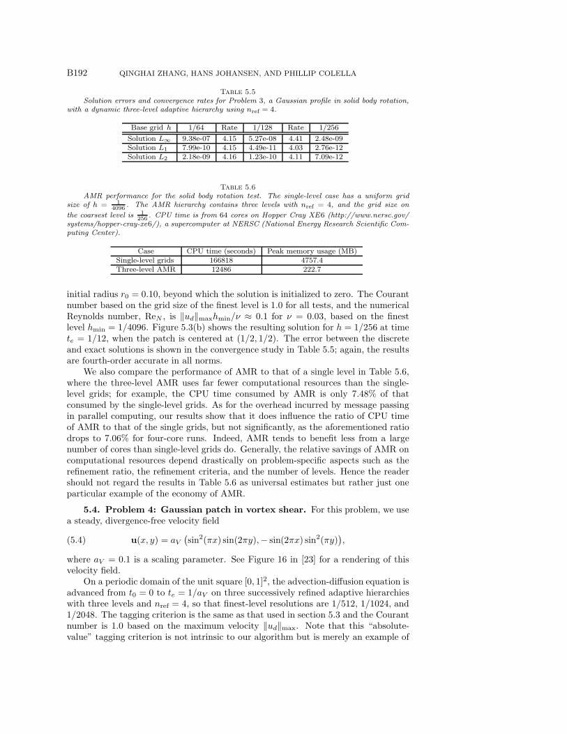
Table 5.5

Solution errors and convergence rates for Problem 3, a Gaussian profile in solid body rotation,with a dynamic three-level adaptive hierarchy using nref = 4.


Solution L∞ 9.38e-07 4.15 5.27e-08 4.41 2.48e-09Solution L1 7.99e-10 4.15 4.49e-11 4.03 2.76e-12Solution L2 2.18e-09 4.16 1.23e-10 4.11 7.09e-12

Table 5.6

AMR performance for the solid body rotation test. The single-level case has a uniform gridsize of h = 1

4096. The AMR hierarchy contains three levels with nref = 4, and the grid size on

the coarsest level is 1256

. CPU time is from 64 cores on Hopper Cray XE6 (http://www.nersc.gov/systems/hopper-cray-xe6/), a supercomputer at NERSC (National Energy Research Scientific Com-puting Center).

Case CPU time (seconds) Peak memory usage (MB)Single-level grids 166818 4757.4Three-level AMR 12486 222.7

initial radius r0 = 0.10, beyond which the solution is initialized to zero. The Courantnumber based on the grid size of the finest level is 1.0 for all tests, and the numericalReynolds number, ReN , is ‖ud‖maxhmin/ν ≈ 0.1 for ν = 0.03, based on the finestlevel hmin = 1/4096. Figure 5.3(b) shows the resulting solution for h = 1/256 at timete = 1/12, when the patch is centered at (1/2, 1/2). The error between the discreteand exact solutions is shown in the convergence study in Table 5.5; again, the resultsare fourth-order accurate in all norms.

We also compare the performance of AMR to that of a single level in Table 5.6,where the three-level AMR uses far fewer computational resources than the single-level grids; for example, the CPU time consumed by AMR is only 7.48% of thatconsumed by the single-level grids. As for the overhead incurred by message passingin parallel computing, our results show that it does influence the ratio of CPU timeof AMR to that of the single grids, but not significantly, as the aforementioned ratiodrops to 7.06% for four-core runs. Indeed, AMR tends to benefit less from a largenumber of cores than single-level grids do. Generally, the relative savings of AMR oncomputational resources depend drastically on problem-specific aspects such as therefinement ratio, the refinement criteria, and the number of levels. Hence the readershould not regard the results in Table 5.6 as universal estimates but rather just oneparticular example of the economy of AMR.

5.4. Problem 4: Gaussian patch in vortex shear. For this problem, we usea steady, divergence-free velocity field

(5.4) u(x, y) = aV(sin2(πx) sin(2πy),− sin(2πx) sin2(πy)

),

where aV = 0.1 is a scaling parameter. See Figure 16 in [23] for a rendering of thisvelocity field.

On a periodic domain of the unit square [0, 1]2, the advection-diffusion equation isadvanced from t0 = 0 to te = 1/aV on three successively refined adaptive hierarchieswith three levels and nref = 4, so that finest-level resolutions are 1/512, 1/1024, and1/2048. The tagging criterion is the same as that used in section 5.3 and the Courantnumber is 1.0 based on the maximum velocity ‖ud‖max. Note that this “absolute-value” tagging criterion is not intrinsic to our algorithm but is merely an example of


various possible criteria. In our implementation, a user can customize this criterionaccording to the specific application.

The test is also carried out on a single-level grid with uniform grid size of 1/4096;the results on this fine grid are then used as the “best” solution for calculating errorson the adaptive hierarchies. Based on this single-level grid, the numerical Reynoldsnumber is ReN = ‖ud‖maxhmin/ν ≈ 2.44 × 10−2 for ν = 0.001. This parameter ischosen on purpose to test the stiff stability of the ARK4(3)6L[2]SA scheme. Twosnapshots of the solution on the finest adaptive hierarchy are shown in Figure 5.4, att = 2 and te = 10, and the corrected convergence results are shown in Table 5.7.

Let hi (i = 1, 2, . . . , N) denote the grid size of the finest level in the ith hierarchyand N the total number of successively refined AMR hierarchies. Let r = hi/hi+1 bethe hierarchy refinement ratio. To calculate the convergence rate p from numericalresults of these hierarchies, we first write

φh = φExact + aphp +O(hp+1),

where the coefficient ap is independent of h. Standard Richardson extrapolationestimates the convergence rate via differences between successive hierarchies:

(5.5) p ≈ logr‖φhi − φhi+1‖‖φhi+1 − φhi+2‖

.

Alternatively, a variant of Richardson extrapolation estimates the convergence ratesby treating the finest solution as the “exact” solution. Define

(5.6a) Ei = ‖φhi − φhmin‖, i = 1, 2, . . . , N,

(5.6b) ei =Ei−1

Ei=rp(N−i+2) − 1

rp(N−i+1) − 1, i = 2, . . . , N,

where the grid size of the exact solution is hmin = hN/r, and ei is the computed errorratio of two successive hierarchies. Equation (5.6b) can be solved for rp, and then p.For i = N and i = N − 1, we have

(5.7) p ≈ logr(eN − 1), p ≈ logr

(√e2N−1 + 2eN−1 − 3 + eN−1 − 1

)− 1.

The difference between the estimated convergence rates by (5.5) and (5.7) is negligiblein the asymptotic range, but might be substantial if the grid sizes are not small enough.

In this test, N = 3, r = 2, and we first compute the solution error by (5.6a) andthen the convergence rates by (5.6b) and (5.7). As shown in Table 5.7, the resultingconvergence rates are 4 or greater. Note that the error estimate at the finest grid iseight orders of magnitude smaller (10−8) than the maximum solution value, whichwith the convergence rate would indicate that the convergence is in the asymptoticrange. For the coarsest grid, h = 1/512, the rates are greater than the asymptoticfourth order, which might be an indication of ARK4(3)6L[2]SA losing accuracy dueto stiffness of the system at the largest time step of the coarsest grid, as discussedin [12, 15]. At the coarser grid resolution and time step, the solution is slightlyunderresolved due to the rapid diffusion of the Gaussian peak.


(a) Problem 4 solution at t = 2

(b) Problem 4 solution at t = te = 10

Fig. 5.4. Solution for Problem 4 at two time instances on a three-level adaptive hierarchy. Theinitial condition is a Gaussian blob, the same as that shown in Figure 5.3(a) except that its centeris located at (1/2, 3/4). As it diffuses, the advection velocity stretches and shears the solution at (a)t = 2 and (b) t = 10. Light blue and black boxes represent level 1 and level 2, respectively.


Table 5.7

Solution error (5.6a) and estimated convergence rates (5.7) of Problem 4 at te = 10 withhmin = 1/4096.

Finest grid h 1/512 Rate 1/1024 Rate 1/2048

Solution L∞ 5.75e-06 5.19 1.58e-07 4.06 8.89e-09Solution L1 1.51e-08 5.01 4.71e-10 4.04 2.71e-11Solution L2 2.36e-08 5.05 7.11e-10 4.04 4.06e-11

6. Conclusions and future research. We have presented a fourth-order accu-rate algorithm for solving the advection-diffusion equation with AMR. The algorithm’sAMR-enabled multigrid solver is general and can be applied to Poisson’s equation andthe heat equation in two and three dimensions, with a variety of boundary conditions,without modification. Although the spatial discretization was chosen to be fourth-order accurate, the algorithm—based on approximating fluxes using quadratures—isgeneral and can be extended to higher orders in space and applied across a variety ofgeneralized mixed hyperbolic, elliptic, and parabolic equations. The uniqueness of ourapproach lies in the combination of fourth-order FV stencils, AMR, the ARK timeintegrator, and multigrid solvers, all of which are general and capable of handlingvariable-coefficient problems and are fundamental components of solvers for morecomplicated PDEs.

Our immediate research concern is a fourth-order accurate adaptive algorithmfor solving the incompressible Navier–Stokes equations, using a projection algorithmsuch as a generalization of the one in [13]. For periodic domains, we expect this tobe a straightforward task; see [11, 16] for related work. However, in the presence ofsolid-wall boundaries, the lack of commutativity between the Laplacian operator andthe Hodge projection operator is a nontrivial technical barrier [5] to be overcome inextending the present method to that case. In addition, we will need to adapt themethod in [14] to support refinement in time and robust limiters near discontinuities.

Appendix A. From cell-averaged to face-averaged quantities.Face-averaged and cell-averaged quantities can be expressed in terms of point

values with second-order correction terms:

(A.1) 〈φ〉i+ 12e

d = φi+ 12e

d +h2

24

∑d′ �=d

∂2φ

∂x2d′

∣∣∣∣∣∣i+ 1

2 ed

+O(h4)

and

(A.2) 〈φ〉i = φi +h2

24

D∑d=1

∂2φ

∂x2d

∣∣∣∣∣i

+O(h4),

where φi+ 12e

d and φi denote the point values at the center of Ai+ 12e

d and Vi, respec-tively.

The derivation is as follows. Let

(A.3) Φ(x) =

∫ x

ξ

φ(x′) dx′

denote an indefinite integral with its lower limit ξ fixed. The average of φ over theinterval [i− 1

2 , i+12 ]h can be obtained by

(A.4) h 〈φ〉i = δΦi(y) = Φi+ 12− Φi− 1

2= Φ

((i+

1

2

)h

)− Φ

((i− 1

2

)h

).


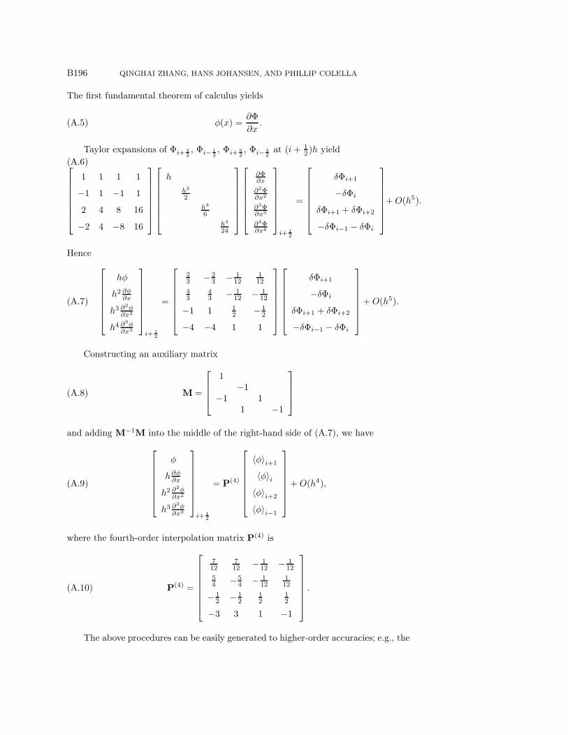
The first fundamental theorem of calculus yields

(A.5) φ(x) =∂Φ

∂x.

Taylor expansions of Φi+ 32, Φi− 1

2, Φi+ 5

2, Φi− 3

2at (i+ 1

2 )h yield

(A.6)⎡⎢⎢⎢⎢⎢⎢⎣

1 1 1 1

−1 1 −1 1

2 4 8 16

−2 4 −8 16

⎤⎥⎥⎥⎥⎥⎥⎦

⎡⎢⎢⎢⎢⎢⎢⎣

h

h2

2

h3

6

h4

24

⎤⎥⎥⎥⎥⎥⎥⎦

⎡⎢⎢⎢⎢⎢⎢⎣

∂Φ∂x

∂2Φ∂x2

∂3Φ∂x3

∂4Φ∂x4

⎤⎥⎥⎥⎥⎥⎥⎦i+ 1

2

=

⎡⎢⎢⎢⎢⎢⎢⎣

δΦi+1

−δΦi

δΦi+1 + δΦi+2

−δΦi−1 − δΦi

⎤⎥⎥⎥⎥⎥⎥⎦+O(h5).

Hence

(A.7)

⎡⎢⎢⎢⎢⎢⎢⎣

hφ

h2 ∂φ∂x

h3 ∂2φ∂x2

h4 ∂3φ∂x3

⎤⎥⎥⎥⎥⎥⎥⎦i+ 1

2

=

⎡⎢⎢⎢⎢⎢⎢⎣

23 − 2

3 − 112

112

43

43 − 1

12 − 112

−1 1 12 − 1

2

−4 −4 1 1

⎤⎥⎥⎥⎥⎥⎥⎦

⎡⎢⎢⎢⎢⎢⎢⎣

δΦi+1

−δΦi

δΦi+1 + δΦi+2

−δΦi−1 − δΦi

⎤⎥⎥⎥⎥⎥⎥⎦+O(h5).

Constructing an auxiliary matrix

(A.8) M =

⎡⎢⎢⎣

1−1

−1 11 −1

⎤⎥⎥⎦

and adding M−1M into the middle of the right-hand side of (A.7), we have

(A.9)

⎡⎢⎢⎢⎢⎢⎢⎣

φ

h∂φ∂x

h2 ∂2φ∂x2

h3 ∂3φ∂x3

⎤⎥⎥⎥⎥⎥⎥⎦i+ 1

2

= P(4)

⎡⎢⎢⎢⎢⎢⎢⎣

〈φ〉i+1

〈φ〉i〈φ〉i+2

〈φ〉i−1

⎤⎥⎥⎥⎥⎥⎥⎦+O(h4),

where the fourth-order interpolation matrix P(4) is

(A.10) P(4) =

⎡⎢⎢⎢⎢⎢⎢⎣

712

712 − 1

12 − 112

54 − 5

4 − 112

112

− 12 − 1

212

12

−3 3 1 −1

⎤⎥⎥⎥⎥⎥⎥⎦.

The above procedures can be easily generated to higher-order accuracies; e.g., the


fifth-order interpolation matrix is

(A.11) P(5) =

⎡⎢⎢⎢⎢⎢⎢⎢⎢⎢⎣

4960

920 − 13

60 − 120

130

54 − 5

4 − 112

112 0

− 94

12

32

14 − 1

4

−3 3 1 −1 0

7 −4 −4 1 1

⎤⎥⎥⎥⎥⎥⎥⎥⎥⎥⎦,

where the additional column is associated with 〈φ〉i+3. Note that the formulas of

fourth order and fifth order coincide for ∂φ∂x .

In a multidimensional space, averaging the first row of (A.9) over all other dimen-sions yields (2.4). Using the second row of (A.11) and averaging an equation similarto (A.9) yield (2.5).

Appendix B. Discrete advection and Laplacian operators.We denote the cell center of Vi by xi =

(i+ 1

21l)h, and the face centers by

xi± 12 e

d = xi ± h2e

d. Let xc = xi+ 12e

d be the center of Ai+ 12e

d . Then the Taylor series

of a function φ about xc can be expressed using standard multi-index notation [9]:

(B.1) φ(x) =∑|j|≤3

1

j!(x− xc)

j φ(j)(xc) +O(h4) =∑|j|≤3

1

j!ηjφ(j)(xc) +O(h4) ,

where η = x− xc, so that ηd = 0 and |η| ≈ O(h) on Ai+ 12e

d .

Then the convolution of two functions φ, ψ : RD → R is

φ(x)ψ(x) =

⎛⎝∑

|j|≤3

1

j!ηjφ(j)(xc)

⎞⎠⎛⎝∑

|k|≤3

1

k!ηkψ(k)(xc)

⎞⎠+O(h4)

=∑

k:|k|≤3

1

k!ηk

∑j:j≤k

(k

j

)φ(j)(xc)ψ

(k−j)(xc) +O(h4),

and the average over Ai+ 12e

d (dropping indices on A and evaluation at xc) is

1

hD−1

∫A

φψ dx =1

hD−1

∫A

∑k:|k|≤3

1

k!ηk

∑j:j≤k

(k

j

)φ(j)ψ(k−j) dx+O(h4)

=∑

k:|k|≤3

1

k!

(1

hD−1

∫A

ηk dx

) ∑j:j≤k

(k

j

)φ(j)ψ(k−j) +O(h4) .

Note that if k is odd in any component or kd = 0, then the contribution of the integralof ηk is 0. Hence, the only nonzero terms come from the choices of k = 0, j = 0 and


k = 2ed′, j = 0, ed

′, 2ed

′with d′ = d. Thus,

1

hD−1

∫A

φψ dx

= φψ +h2

24

∑d′ �=d

(φ(2e

d′ )ψ + ψ(2ed′ )φ)+h2

12

∑d′ �=d

(φ(e

d′ )ψ(ed′ ))+O(h4)

=

(φ+

h2

24

∑d′ �=d

φ(2ed′ ))(

ψ +h2

24

∑d′ �=d

ψ(2ed′))+h2

12

∑d′ �=d

(φ(e

d′ )ψ(ed′ ))+O(h4)

= 〈φ〉i+ 12e

d 〈ψ〉i+ 12e

d +h2

12

∑d′ �=d

(φ(e

d′ )ψ(ed′ ))+O(h4) ,

where we have used (A.1) to convert the first two terms in parentheses to face-averagedquantities.

The last term, representing the product of “transverse gradients,” can be approx-imated with

G⊥d′φ

∣∣i+ 1

2ed =

1

2h

(〈φ〉i+ 1

2ed+ed′ − 〈φ〉i+ 1

2ed−ed′

)=

∂φ

∂xd′

∣∣∣∣i+ 1

2 ed

+O(h2) ,

leading to O(h4) overall for the average flux formula:(B.2)

〈φψ〉i+ 12e

d = 〈φ〉i+ 12e

d 〈ψ〉i+ 12e

d+h2

12

∑d′ �=d

(G⊥

d′φ∣∣i+ 1

2 ed G

⊥d′ψ

∣∣i+ 1

2ed

)+C3(xi+ 1

2ed)h4+O(h5).

Substituting ud for ψ yields the discrete advection operator in (2.6a); the O(h4)accuracy in (2.6a) is due to the cancellation caused by the symmetry of the differencestencils, i.e., C3(xi+ 1

2ed)− C3(xi− 1

2ed) = O(h).

As for the discrete Laplacian operator, we identify �F = ∇φ in (1.1) to obtain

(B.3) 〈Δφ〉i =1

h

D∑d=1

(⟨∂φ

∂xd

⟩i+ 1

2 ed

−⟨∂φ

∂xd

⟩i− 1

2ed

).

From the second row of the fifth-order interpolation matrix (A.11), we have⟨∂φ

∂x

⟩i+ 1

2ed

=1

12h

(15 〈φ〉i+ed−15 〈φ〉i−〈φ〉i+2ed+〈φ〉i−ed

)+C4

(xi+ 1

2 ed

)h4+O(h5),

which leads to an equation identical to (2.7):

〈Δφ〉i =1

12h2

D∑d=1

(16 〈φ〉i+ed + 16 〈φ〉i−ed − 30 〈φ〉i − 〈φ〉i+2ed − 〈φ〉i−2ed

)+O(h4),

where we have used the fact that

C4(xi+ 12e

d)− C4(xi− 12 e

d) = h∂C4

∂xd

∣∣∣∣xi

+O(h3).

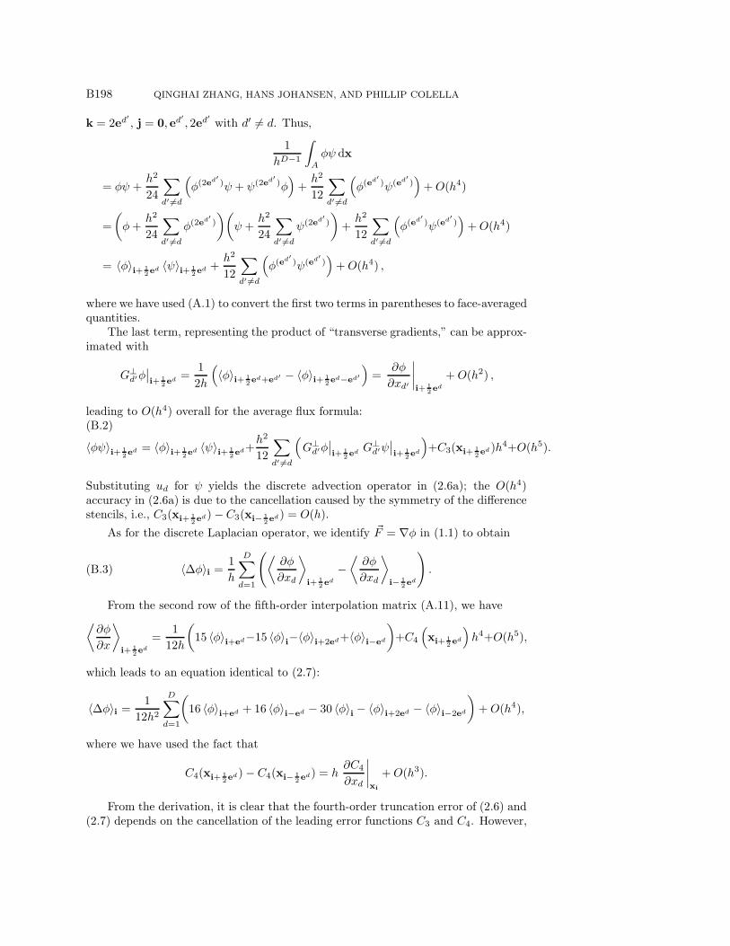
From the derivation, it is clear that the fourth-order truncation error of (2.6) and(2.7) depends on the cancellation of the leading error functions C3 and C4. However,


for a coarse cell close to the coarse-fine interface where the coarse flux is replaced bythe average of the fine fluxes, the truncation error is only third-order accurate due tothe lack of this cancellation.

Appendix C. ARK4 coefficients. Kennedy and Carpenter [12] studied a groupof implicit-explicit Runge–Kutta schemes from third- to fifth-order accurate with thefollowing form:

(C.1)

c[E] A[E]

(b[E]

)T(b[E])T

=

0 0 0 0 · · · 0 0

2γ 2γ 0 0 · · · 0 0

c3 a[E]31 a

[E]32 0 · · · 0 0

......

......

. . ....

...

cs−1 a[E]s−1,1 a

[E]s−1,2 a

[E]s−1,3 · · · 0 0

1 a[E]s,1 a

[E]s,2 a

[E]s,3 · · · a

[E]s,s−1 0

b1 b2 b3 · · · bs−1 γ

b1 b2 b3 · · · bs−1 bs

,

(C.2)

c[I] A[I]

(b[I]

)T(b[I])T

=

0 0 0 0 · · · 0 0

2γ γ γ 0 · · · 0 0

c3 a[I]31 a

[I]32 γ · · · 0 0

......

......

. . ....

...

cs−1 a[I]s−1,1 a

[I]s−1,2 a

[I]s−1,3 · · · γ 0

1 b1 b2 b3 · · · bs−1 γ

b1 b2 b3 · · · bs−1 γ

b1 b2 b3 · · · bs−1 bs

.

The coefficients of the particular method used in this work, ARK4(3)6L[2]SA,are, in decimal form [20], γ = 0.25, c[E] = c[I] = c, b[E] = b[I] = b,

c = (0.0, 0.5, 0.332, 0.62, 0.85, 1.0)T ,

b1 = 0.15791629516167136,

b2 = 0,

b3 = 0.18675894052400077,

b4 = 0.6805652953093346,

b5 = −0.27524053099500667,


a[E]31 = 0.221776,

a[E]32 = 0.110224,

a[E]41 = −0.04884659515311857,

a[E]42 = −0.17772065232640102,

a[E]43 = 0.8465672474795197,

a[E]51 = −0.15541685842491548,

a[E]52 = −0.3567050098221991,

a[E]53 = 1.0587258798684427,

a[E]54 = 0.30339598837867193,

a[E]61 = 0.2014243506726763,

a[E]62 = 0.008742057842904185,

a[E]63 = 0.15993995707168115,

a[E]64 = 0.4038290605220775,

a[E]65 = 0.22606457389066084,

a[I]31 = 0.137776,

a[I]32 = −0.055776,

a[I]41 = 0.14463686602698217,

a[I]42 = −0.22393190761334475,

a[I]43 = 0.4492950415863626,

a[I]51 = 0.09825878328356477,

a[I]52 = −0.5915442428196704,

a[I]53 = 0.8101210538282996,

a[I]54 = 0.283164405707806.

Acknowledgments. The first author, Qinghai Zhang, would like to thank DanGraves, Terry Ligocki, Dan Martin, Peter McCorquodale, Peter Schwartz, David Tre-botich, and Brian Van Straalen for helpful discussions during the process of this work.

REFERENCES

[1] M. Barad and P. Colella, A fourth-order accurate local refinement method for Poisson’sequation, J. Comput. Phys., 209 (2005), pp. 1–18.

[2] M. J. Berger and P. Colella, Local adaptive mesh refinement for shock hydrodynamics, J.Comput. Phys., 82 (1989), pp. 64–84.

[3] A. Brandt, Algebraic multigrid theory: The symmetric case, Appl. Math. Comput., 19 (1986),pp. 23–56.

[4] W. L. Briggs, V. E. Henson, and S. F. McCormick, A Multigrid Tutorial, 2nd ed., SIAM,Philadelphia, 2000.

[5] D. L. Brown, R. Cortez, and M. L. Minion, Accurate projection methods for the incom-pressible Navier-Stokes equations, J. Comput. Phys., 168 (2001), pp. 464–499.


[6] M. P. Calvo, J. de Frutos, and J. Novo, Linearly implicit Runge-Kutta methods foradvection-reaction-diffusion equations, Appl. Numer. Math., 37 (2001), pp. 535–549.

[7] P. Colella, M. R. Dorr, J. A. F. Hittinger, and D. F. Martin, High-order, finite-volumemethods in mapped coordinates, J. Comput. Phys., 230 (2011), pp. 2952–2976.

[8] P. Colella and P. R. Woodward, The piecewise parabolic method (PPM) for gas-dynamicalsimulations, J. Comput. Phys., 54 (1984), pp. 174–201.

[9] L. C. Evans, Partial Differential Equations, American Mathematical Society, Providence, RI,1998.

[10] H. Johansen and P. Colella, A Cartesian grid embedded boundary method for Poisson’sequation on irregular domains, J. Comput. Phys., 147 (1998), pp. 60–85.

[11] S. Y. Kadioglu, R. Klein, and M. L. Minion, A fourth-order auxiliary variable projectionmethod for zero-Mach number gas dynamics, J. Comput. Phys., 227 (2009), pp. 2012–2043.

[12] C. A. Kennedy and M. H. Carpenter, Additive Runge-Kutta schemes for convection-diffusion-reaction equations, Appl. Numer. Math., 44 (2003), pp. 139–181.

[13] D. F. Martin, P. Colella, and D. Graves, A cell-centered adaptive projection method forthe incompressible Navier-Stokes equations in three dimensions, J. Comput. Phys., 227(2008), pp. 1863–1886.

[14] P. McCorquodale and P. Colella, A high-order finite-volume method for hyperbolic con-servation laws on locally refined grids, Commun. Appl. Math. Comput. Sci., 6 (2011),pp. 1–25.

[15] M. L. Minion, Semi-implicit spectral deferred correction methods for ordinary differential equa-tions, Commun. Math. Sci., 1 (2003), pp. 471–500.

[16] M. L. Minion, Semi-implicit projection methods for incompressible flow based on spectral de-ferred corrections, Appl. Numer. Math., 48 (2004), pp. 369–387.

[17] K. W. Morton, Numerical Solution of Convection-Diffusion Problems, Appl. Math. Math.Comput. 12, Chapman & Hall, London, 1996.

[18] M. Stynes, Steady-state convection-diffusion problems, Acta Numer., 14 (2005), pp. 445–508.[19] U. Trottenberg, C. W. Oosterlee, and A. Schuller, Multigrid, Academic Press, San

Diego, CA, 2001.[20] J. Wilkening, Math 228A: Numerical Solutions of Differential Equations, lecture notes,

http://math.berkeley.edu/∼wilken/228A.F07/ (2007).[21] S. T. Zalesak, A physical interpretation of the Richtmyer two-step Lax-Wendroff scheme,

and its generalization to higher spatial order, in Advances in Computer Methods for Par-tial Differential Equations V, R. Vichnevetsky and R. S. Stepleman, eds., Proceedings ofthe Fifth IMACS International Symposium on Computer Methods for Partial DifferentialEquations, 1984, pp. 491–496.

[22] Q. Zhang, High-order, multidimensional, and conservative coarse-fine interpolation for adap-tive mesh refinement, Comput. Methods Appl. Mech. Engrg., 200 (2011), pp. 3159–3168.

[23] Q. Zhang and P. L.-F. Liu, A new interface tracking method: The polygonal area mappingmethod, J. Comput. Phys., 227 (2008), pp. 4063–4088.

[24] Q. Zhang and P. L.-F. Liu, Handling solid-fluid interfaces for viscous flows: Explicit jumpapproximation vs. ghost cell approaches, J. Comput. Phys., 229 (2010), pp. 4225–4246.

a fourth-order accurate finite-volume method with structured

Documents