a framework for learning predictive structures from multiple tasks
TRANSCRIPT
Journal of Machine Learning Research 6 (2005) 1817–1853 Submitted 5/05; Revised 8/05; Published 11/05
A Framework for Learning Predictive Structures from
Multiple Tasks and Unlabeled Data
Rie Kubota Ando [email protected] T.J. Watson Research CenterYorktown Heights, NY 10598, U.S.A.
Tong Zhang [email protected]
Yahoo Research
New York, NY, U.S.A.
Editor: Peter Bartlett
Abstract
One of the most important issues in machine learning is whether one can improve theperformance of a supervised learning algorithm by including unlabeled data. Methods thatuse both labeled and unlabeled data are generally referred to as semi-supervised learning.Although a number of such methods are proposed, at the current stage, we still don’t havea complete understanding of their effectiveness. This paper investigates a closely relatedproblem, which leads to a novel approach to semi-supervised learning. Specifically weconsider learning predictive structures on hypothesis spaces (that is, what kind of classifiershave good predictive power) from multiple learning tasks. We present a general frameworkin which the structural learning problem can be formulated and analyzed theoretically, andrelate it to learning with unlabeled data. Under this framework, algorithms for structurallearning will be proposed, and computational issues will be investigated. Experiments willbe given to demonstrate the effectiveness of the proposed algorithms in the semi-supervisedlearning setting.
1. Introduction
In machine learning applications, one can often find a large amount of unlabeled datawithout difficulty, while labeled data are costly to obtain. Therefore a natural questionis whether we can use unlabeled data to build a more accurate classifier, given the sameamount of labeled data. This problem is often referred to as semi-supervised learning.
In general, semi-supervised learning algorithms use both labeled and unlabeled data totrain a classifier. Although a number of methods have been proposed, their effectivenessis not always clear. For example, Vapnik introduced the notion of transductive inference(Vapnik, 1998), which may be regarded as an approach to semi-supervised learning. Al-though some success has been reported (e.g., see Joachims, 1999), there has also beencriticism pointing out that this method may not behave well under some circumstances(Zhang and Oles, 2000). Another popular semi-supervised learning method is co-training(Blum and Mitchell, 1998), which is related to the bootstrap method used in some NLPapplications (Yarowsky, 1995) and to EM (Nigam et al., 2000). The basic idea is to labelpart of unlabeled data using a high precision classifier, and then put the “automatically-
c©2005 Rie Kubota Ando and Tong Zhang.
Ando and Zhang
labeled” data into the training data. However, it was pointed out by Pierce and Cardie(2001) that this method may degrade the classification performance when the assumptionsof the method are not satisfied (that is when noise is introduced into the labels throughnon-perfect classification). This phenomenon is also observed in some of our experimentsreported in Section 5.
Another approach to semi-supervised learning is based on a different philosophy. Thebasic idea is to define good functional structures using unlabeled data. Since it does notbootstrap labels, there is no label noise which can potentially corrupt the learning procedure.An example of this approach is to use unlabeled data to create a data-manifold (graphstructure), on which proper smooth function classes can be defined (Szummer and Jaakkola,2002; Zhou et al., 2004; Zhu et al., 2003). If such smooth functions can characterize theunderlying classifier very well, then one is able to improve the classification performance.
It is worth pointing out that smooth function classes based on graph structures do notnecessarily have good predictive power. Therefore a more general approach, based on thesame underlying principle, is to directly learn a good underlying smooth function class (thatis, what good classifiers are like). If the learning procedure takes advantage of unlabeleddata, then we obtain a semi-supervised learning method that is specifically aimed at findingstructures with good predictive power.
This motivates the general framework we are going to develop in this paper. That is,we want to learn some underlying predictive functional structures (smooth function classes)that can characterize what good predictors are like. We call this problem structural learn-ing. Our key idea is to learn such structures by considering multiple prediction problemssimultaneously. At the intuitive level, when we observe multiple predictors for differentproblems, we have a good sample of the underlying predictor space, which can be analyzedto find the common structures shared by these predictors. Once important predictive struc-tures on the predictor space are discovered, we can then use the information to improveupon each individual prediction problem. A main focus of this paper is to formalize thisintuitive idea and analyze properties of structural learning more rigorously.
The idea that one can benefit by considering multiple problems together has appearedin the statistical literature. In particular, Bayesian hierarchical modeling is motivated fromthe same principle. However, the framework developed in this paper is under the frequentistsetting, and the most relevant statistical studies are shrinkage methods in multiple-outputlinear models (see Section 3.4.6 of Hastie et al., 2001). In particular, the algorithm proposedin Section 3 has a form similar to a shrinkage method proposed by Breiman and Friedman(1997). However, the framework presented here (as well as the specific algorithm in Sec-tion 3) is more general than the earlier statistical studies. In the machine learning literature,related work is sometime referred to as multi-task learning, for example, see (Baxter, 2000;Ben-David and Schuller, 2003; Caruana, 1997; Evegniou and Pontil, 2004; Micchelli andPonti, 2005) and references therein. We shall call our procedure structural learning since itis a more accurate description of what our method does in the semi-supervised learning set-ting. That is, we transfer the predictive structure learned from multiple tasks (on unlabeleddata) to the target supervised problem. In the literature, this idea is also referred to asinductive transfer. The success of this approach depends on whether the learned structureis helpful for the target supervised problem.
1818
Learning Predictive Structures
It follows that although this work is motivated by semi-supervised learning, the generalstructural learning (or multi-task learning) problem considered in the paper is of indepen-dent interest. For semi-supervised learning, as we shall show later, the multiple predictionproblems needed for structural learning can be generated from unlabeled data. However,the basic framework can also be applied to other applications where we have multiple pre-diction problems that are not necessarily derived from unlabeled data (as in the earlierstatistical and machine learning studies). Because of this, the first part of the paper focuseson the development of a general structural learning paradigm as well as our algorithm. Themain implication is that one can reliably learn a good underlying structure if it is shared bymultiple prediction problems. In the second part, we shall demonstrate how to apply theidea of learning structure to semi-supervised learning, and demonstrate the effectiveness ofthe proposed method in this context.
A short version of this paper, mainly reporting some empirical results, appeared inACL (Ando and Zhang, 2005). This version includes a more complete derivation of theproposed algorithm, with theoretical analysis and several additional experimental results.In Section 2, we formally introduce the structural learning problem under the frameworkof standard machine learning. We then propose a specific algorithm that finds a commonlow-dimensional feature space shared by the multi-problems. The algorithm will be stud-ied in Section 3, with theoretical analysis given in Appendix A. Section 4 shows how toapply structural learning in the context of semi-supervised learning. The basic idea is touse unlabeled data to generate auxiliary prediction problems that are useful for discoveringimportant predictive structures. Such structures can then be estimated using the algorithmdeveloped in Section 3. We will also give intuitive justifications on why the structure sharedby the artificially created auxiliary problems is helpful for the supervised problem. Experi-ments are provided in Section 5 to illustrate the effectiveness of the algorithm proposed inSection 3 on several semi-supervised tasks. Section 6 presents a high level summary of themain ideas developed in the paper.
2. The Structural Learning Problem
This section introduces the problem of learning predictive functional structures. Althoughrelated ideas have been explored in some earlier statistical and machine learning studies,for completeness, we shall include a self-contained description. The framework consideredhere will be the basis of our algorithm presented in Section 3.
2.1 Supervised Learning
In the standard formulation of supervised learning, we seek a predictor that maps an inputvector x ∈ X to the corresponding output y ∈ Y. Usually, one selects the predictor from aset H of functions based on a finite set of training examples {(Xi, Yi)} that are independentlygenerated according to some unknown probability distribution D. The set H, often calledthe hypothesis space, consists of functions from X to Y that can be used to predict theoutput in Y of an input datum in X . Our goal is to find a predictor f so that its errorwith respect to D is as small as possible. In this paper, we assume that the quality of the
1819
Ando and Zhang
predictor p is measured by the expected loss with respect to D:
R(f) = EX,Y L(f(X), Y ).
Given a set of training data, a frequently used method for finding a predictor f ∈ H is tominimize the empirical error on the training data (often called empirical risk minimizationor ERM):
f = arg minf∈H
n∑
i=1
L(f(Xi), Yi).
It is well-known that with a fixed sample size, the smaller the hypothesis space H, theeasier it is to learn the best predictor in H. The error caused by learning the best predictorfrom finite sample is called the estimation error. However, the smaller the hypothesis spaceH, the less accurate the best predictor in H becomes. The error caused by using a restrictedH is often referred to as the approximation error. In supervised learning, one needs to selectthe size of H to balance the trade-off between approximation error and estimation error.This is typically done through model selection, where we learn a set of predictors from aset of candidate hypothesis spaces Hθ, and then pick the best choice on a validation set.
2.2 Learning Good Hypothesis Spaces
In practice, a good hypothesis space should have a small approximation error and a smallestimation error. The problem of choosing a good hypothesis space is central to the perfor-mance of the learning algorithm, but often requires specific domain knowledge or assump-tions of the world.
Assume that we have a set of candidate hypothesis spaces. If one only observes a singleprediction problem X → Y on the underlying domain X , then a standard approach tohypothesis space selection (or model selection) is by cross validation. If one observes multipleprediction problems on the same underlying domain, then it is possible to make betterestimate of the underlying hypothesis space by considering these problems simultaneously.
We now describe a simple model for structural learning, which is the foundation ofthis paper. A similar point of view can also be found in (Baxter, 2000). Consider mlearning problems indexed by ` ∈ {1, . . . , m}, each with n` samples (X`
i , Y`i ) indexed by
i ∈ {1, . . . , n`}, which are independently drawn from a distribution D`. For each problem`, assume that we have a set of candidate hypothesis spaces H`,θ indexed by a commonstructural parameter θ ∈ Γ that is shared among the problems.
Now, for the `-th problem, we are interested in finding a predictor f` : X → Y inH`,θ that minimizes the expected loss over D`. For notational simplicity, we assume thatthe problems have the same loss function (although the requirement is not essential in ouranalysis). Given a fixed structural parameter θ, the predictor for each problem can beestimated using empirical risk minimization (ERM) over the hypothesis space H`,θ:
f`,θ = arg minf∈H`,θ
n∑
i=1
L(f(X`i), Y
`i ), (` = 1, . . . , m). (1)
The purpose of structural learning is to find an optimal structural parameter θ such thatthe expected risks of the predictors f`,θ (each with respect to the corresponding distributionD`), when averaged over ` = 1, . . . , m, are minimized.
1820
Learning Predictive Structures
If we use cross-validation for structural parameter selection, then we can immediatelynotice that a more stable estimate of the optimal θ can be obtained by considering multiplelearning tasks together. In particular, if for each problem `, we have a validation set(X`
j , Y`j ) for j = 1, . . . , n`, then for structural learning, the total number of validation data
is∑m
`=1 n`. Therefore effectively, we have more data for the purpose of selecting the optimalshared hypothesis space structure. This implies that even if the sample sizes are small forthe individual problems, as long as m is large, we are able to find the optimal θ accurately.A PAC style analysis will be provided in Appendix A, where we can state a similar resultwithout cross-validation.
In general, we expect that the hypothesis space H`,θ determines the functional structureof the learned predictor. The θ parameter can be a continuous parameter that encodes ourassumption of what a good predictor should be like. If we have a large parameter space,then we can explore many possible functional structures. This argument (more rigorousresults are given in Appendix A) implies that it is possible to discover the optimal sharedstructure when the number of problems m is large.
2.3 Good Structures on the Input Space
The purpose of this section is to provide an intuitive discussion on why in principle, thereexist good functional structures (good hypothesis spaces) shared by multiple tasks. Concep-tually, we may consider the simple case H`,θ = Hθ, where different problems share exactlythe same underlying hypothesis space.
Given an arbitrary input space X without any known structure, we argue that it is oftenpossible to learn what a good predictor looks like from multiple prediction problems. Thekey reason is that in practice, not all predictors are equally good (or equally likely to beobserved). In real world applications, one usually observes “smooth” predictors where thesmoothness is with respect to a certain intrinsic underlying distance on the input space.In general, if two points are close in this intrinsic distance, then the values that a goodpredictor produces at these points are also likely to be similar. In particular, completelyrandom predictors are likely to be bad predictors, and are rarely observed in practicalapplications.
In machine learning, the smoothness condition is often enforced by the hypothesis spacewe select. For example, kernel methods constrain the smoothness of a function using acertain reproducing kernel Hilbert space (RKHS) norm. For such functions (in a RKHS),closeness of two points under a certain metric often implies closeness in predictive values.One may also consider more complicated smoothness conditions that explore the observeddata-manifold (e.g. graph-based semi-supervised learning methods mentioned in the intro-duction). Such a smoothness condition will be useful if it correlates well with predictiveability.
In general, a good distance measure on X induces a good hypothesis space which enforcessmoothness with respect to the underlying distance. However, in reality, it is often notclear what is the best distance measure in the underlying space. For example, in naturallanguage processing, the space X consists of discrete points such as words, for which noappropriate distance can be easily defined. Even for continuous vector-valued input points,it is difficult to justify that the Euclidean distance is better than something else. Even after
1821
Ando and Zhang
a good distance function can be selected, it is not clear whether we can define appropriatesmoothness conditions with respect to the distance.
If we observe multiple tasks, then important common structures can be discovered simplyby analyzing the multiple predictors learned from the data. If these tasks are very similarto the actual learning task which we are interested in, then we can benefit significantlyfrom the discovered structures. Even if the tasks are not directly related, the discoveredstructures can still be useful. This is because in general, predictors tend to share similarsmoothness conditions with respect to a certain distance that is intrinsic to the underlyinginput space.
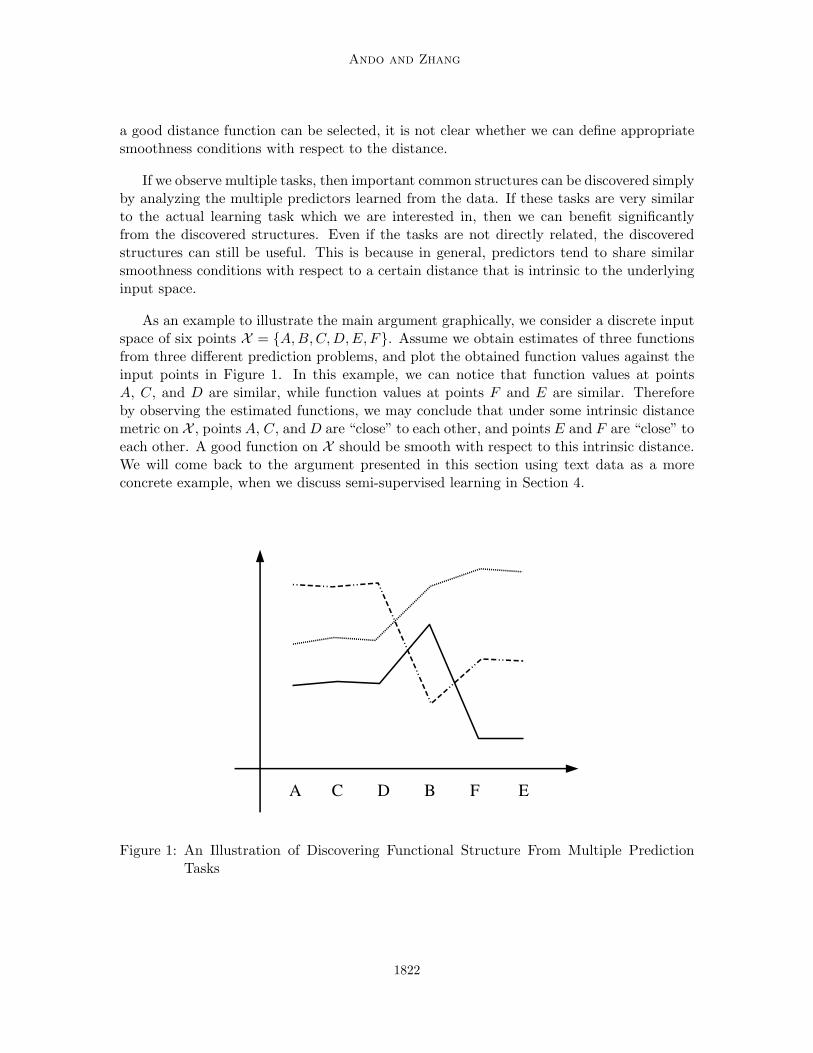
As an example to illustrate the main argument graphically, we consider a discrete inputspace of six points X = {A, B, C, D, E, F}. Assume we obtain estimates of three functionsfrom three different prediction problems, and plot the obtained function values against theinput points in Figure 1. In this example, we can notice that function values at pointsA, C, and D are similar, while function values at points F and E are similar. Thereforeby observing the estimated functions, we may conclude that under some intrinsic distancemetric on X , points A, C, and D are “close” to each other, and points E and F are “close” toeach other. A good function on X should be smooth with respect to this intrinsic distance.We will come back to the argument presented in this section using text data as a moreconcrete example, when we discuss semi-supervised learning in Section 4.
Figure 1: An Illustration of Discovering Functional Structure From Multiple PredictionTasks
1822
Learning Predictive Structures
2.4 A More Abstract Form of Structural Learning
We may also pose structural learning in a slightly more abstract form, which is useful whenwe don’t use empirical risk minimization as the learner.
Assume that for each problem `, we are given a learning algorithm A` that takes a setof training samples S` = {(X`
i , Y`i )}i=1,...,n`
and a structural parameter θ ∈ Γ, and produce
a predictor f`,θ: f`,θ = A`(S`, θ). Note that if the algorithm estimates the predictor from a
hypothesis space H`,θ by empirical risk minimization, then we have f`,θ ∈ H`,θ.
Assume further that there is a procedure that estimates the performance of the learnedpredictor f`,θ using possibly additional information T` (which for example, could be a val-
idation set) as O`(S`, T`, θ). Then in structural learning, we find θ by using a regularizedestimator
θ = arg minθ∈Γ
[
r(θ) +m∑
`=1
O`(S`, T`, θ)
]
, (2)
where r(θ) is a regularization parameter that encodes our belief on what θ value is preferred.The number of problems m behaves like the sample size in standard learning. This is ourfundamental estimation method for structural learning. Once we obtain an estimate θ ofthe structural parameter, we can use the learning algorithm A`(S`, θ) to obtain predictorf`,θ for each `.
As an example, assume that we estimate the accuracy of f`,θ using a validation set
T` = {(X`j , Y
`j )}j=1,...,n`
, then we may simply let O(S`, T`, θ) = α`∑n`
j=1 L(f`,θ(X`j), Y
`j ),
where α` > 0 are weighting parameters. It is also possible to estimate the accuracy of thelearned predictor based on the training set alone using the standard learning theory forempirical risk minimization. This approach will be employed in Section 3, and leads topractical algorithms that can be formulated as optimization problems.
3. Algorithms
In this section, we develop a specific learning algorithm under the standard machine learningframework. The basis of our learner is joint empirical risk minimization, which will be an-alyzed in Appendix A. We consider linear prediction models since they have been shown tobe effective in many practical applications. These methods include state-of-the-art machinelearning algorithms such as kernel machines and boosting.
3.1 Joint Empirical Risk Minimization
Based on the framework outlined in Section 2, we are interested in finding a hypothesis spaceH·,θ, using an estimator of the form (2). As being pointed out in Section 2, conceptuallythis could be achieved using a validation set. However, such an approach can lead to aquite difficult computational procedure since we have to optimize the empirical risk on thetraining data for each possible value of θ, and then choose an optimal θ on the validationset. Therefore for complicated structures with continuous θ parameter such as the modelwe consider in Section 3, this approach is not feasible.
A more natural method is to perform a joint optimization on the training set, withrespect to both the predictors {f`}, and the structural parameter θ. To this end, we will
1823
Ando and Zhang
consider the model given by equation (1), and pose it as a joint optimization problem overthe m problems, where θ is the shared structural parameter:
[θ, {f`}] = arg minθ∈Γ,{f`∈H`,θ}
m∑
`=1
1
n`
n∑
i=1
L(f`(X`i), Y
`i ). (3)
Since the shared structural parameter θ depends on m problems, it can be more reliablyestimated by joint minimization. For completeness, we include a theoretical analysis inAppendix A.
3.2 Structural Learning with Linear Predictors
In order to derive a practical algorithm from (3), we shall consider a specific joint modelwhich can be solved numerically. Specifically, we employ linear prediction models for themultiple tasks, and assume that the underlying structure is a shared low-dimensional sub-space. Although not necessarily most general, this model leads to a simple and intuitivecomputational procedure. As we shall also see later, it is quite effective for semi-supervisedlearning problems that we are interested in.
Given the input space X , a linear predictor is not necessarily linear on the original space,but rather can be regarded as a linear functional on a high dimensional feature space F .We assume there is a known feature map Φ : X → F . A linear predictor f is determined bya weight vector w: f(x) = wTΦ(x). In order to apply the structural learning framework,we consider a parameterized family of feature maps. In this setting, the goal of structurallearning may be regarded as learning a good feature map. For the specific formulation whichwe consider in this paper, we assume that the overall feature map contains two components:one component is with a known high-dimensional feature map, and the other component isa parameterized low-dimensional feature map. That is, the linear predictor has a form
f(x) = wTΦ(x) + vTΨθ(x),
where w and v are weight vectors specific for each prediction problem, and θ is the commonstructure parameter shared by all problems.
In order to simplify numerical computation, we further consider a simple linear form offeature map, where θ = Θ is an h × p dimensional matrix, and Ψθ(x) = ΘΨ(x), with Ψ aknown p-dimensional vector function. We now can write the linear predictor as:
fΘ(w,v;x) = wTΦ(x) + vT ΘΨ(x).
This hypothesis space (with appropriate regularization conditions) is analyzed in Appendix Aafter Theorem 4. We point out there that the key idea of this formulation is to discover ashared low-dimensional predictive structure parameterized by Θ.
Applying (2) with O(S`, T`, θ) given by regularized empirical risk, we obtain the followingformulation:
[{w`, v`}, Θ] = arg min{w`,v`},Θ
[
r(Θ) +m∑
`=1
(
g(w`,v`) +1
n`
n∑
i=1
L(fΘ(w`,v`;X`i), Y
`i )
)]
, (4)
1824
Learning Predictive Structures
where g(w,v) is an appropriate regularization condition on the weight vector (w,v), andr(Θ) is an appropriate regularization condition on the structural parameter Θ. In this for-mulation, we weight each problem equally (by dividing the number of instances n`) so thatno problem will dominate the others. One may also choose other weighting schemes. Notethat the regularized ERM method in (4) has the same form as (3). The main differenceis that we replaced the hard-constrained regularization (picking the predictors from a hy-pothesis space) by its computationally more convenient version of penalized regularization.Up to appropriately defined Lagrangian multipliers, these two formulations are equivalent.
If we consider kernel learning, and assume that the feature map Φ(x) belongs to areproducing kernel Hilbert space, then equation (4) can be kernelized. There are severalways to do so. One possibility is to kernelize in the w parameter — we simply replacethe vector parameter w` by n` dual parameters α`
j (j = 1, . . . , n`), and the linear score
wT` Φ(X`
i) by∑n`
j=1 α`jK(X`
j ,X`i). For simplicity, we do not consider kernel methods in this
paper.
3.3 Alternating Structure Optimization
It is possible to solve (4) using general purpose optimization methods. However, in thissection, we show that by exploring the special structure of the formulation, we can developa more interesting and conceptually appealing computational procedure. In general, weshould pick L and g such that the formulation is convex for fixed Θ. However, the jointoptimization over {w`,v`} and Θ will become non-convex. Therefore, one typically can onlyfind a local minimum with respect to Θ. This usually doesn’t lead to serious problems sincegiven the local optimal structural parameter Θ, the solution {w`,v`} will still be globallyoptimal for every `. Moreover, the algorithm which we propose later in section uses SVDfor dimension reduction. At the conceptual level, the possible local optimality of Θ is nota major issue simply because the SVD procedure itself is already good at finding globallyoptimal low dimensional structure.
With fixed Θ, the computation of {w`,v`} for each problem ` becomes decoupled, andvarious optimization algorithms can be applied for this purpose. The specific choice ofsuch algorithms is not important for the purpose of this paper. In our experiments, forconvenience and simplicity, we employ stochastic gradient descent (SGD), widely used inthe neural networks literature. It was recently argued that this simple method can alsowork well for large scale convex learning formulations (Zhang, 2004).
In the following, we consider a special case of (4) which has a simple iterative SVDsolution. Let Φ(x) = Ψ(x) = x ∈ Rp with square regularization of weight vectors. Thenwe have
[{w`, v`}, Θ] = arg min{w`,v`},Θ
m∑
`=1
(
1
n`
n∑
i=1
L((w` + ΘTv`)TX`
i , Y`i ) + λ`‖w`‖2
2
)
, (5)
s.t. ΘΘT = Ih×h ,
with given constants {λ`}. Note that in this formulation, the regularization condition r(Θ)in (4) is absorbed into the orthonormal constraint ΘΘT = Ih×h, and thus does not need tobe explicitly included.
1825
Ando and Zhang
In order to solve this optimization problem, we may introduce an auxiliary variable u`
for each problem ` such that u` = w` + ΘTv`. Therefore we may eliminate w using u toobtain:
[{u`, v`}, Θ] = arg min{u`,v`},Θ
m∑
`=1
(
1
n`
n∑
i=1
L(uT` X`
i , Y`i ) + λ`‖u` − ΘTv`‖2
2
)
, (6)
s.t. ΘΘT = Ih×h .
At the optimal solution, we let w` = u` − ΘT v`.In order to solve (6), we use the following alternating optimization procedure:
• Fix (Θ,v), and optimize (6) with respect to u.
• Fix u, and optimize (6) with respect to (Θ,v).
• Iterate until convergence.
One may also propose other alternating optimization procedures. For example, in the firststep, we may fix Θ and optimize with respect to (u,v).
In the alternating optimization procedure outlined above, with a convex choice of L,the first step becomes a convex optimization problem. There are many well-establishedmethods for solving it (as mentioned earlier, we use SGD for its simplicity). We shall focuson the second step, which is crucial for the derivation of our method. It is easy to see thatthe optimization of (6) with fixed {u`} = {u`} is equivalent to the following problem:
[{v`}, Θ] = arg min{v`},Θ
∑
`
λ`‖u` − ΘTv`‖22, s.t. ΘΘT = Ih×h. (7)
Using simple linear algebra, we know that with fixed Θ,
minv`
‖u` − ΘTv`‖22 = ‖u`‖2
2 − ‖Θu`‖22,
and the optimal value is achieved at v` = Θu`. Now by eliminating v` and use the aboveequality, we can rewrite (7) as
Θ = arg maxΘ
m∑
`=1
λ`‖Θu`‖22, s.t. ΘΘT = Ih×h.
Let U = [√
λ1u1, . . . ,√
λmum] be an p × m matrix, we have
Θ = arg maxΘ
tr(ΘUUT ΘT ), s.t. ΘΘT = Ih×h,
where tr(A) is the trace of matrix A. It is well-known that the solution of this problem isgiven by the SVD (singular value decomposition) of U: let U = V1DV T
2 be the SVD of U(assume that the diagonal elements of D are arranged in decreasing order), then the rowsof Θ are given by the first h rows of V T
1 (left singular vectors corresponding to the largest hsingular values of U). We now summarize the above derivation into an algorithm describedin Figure 2, which solves (5) by alternating optimization of u and (Θ,v).
1826
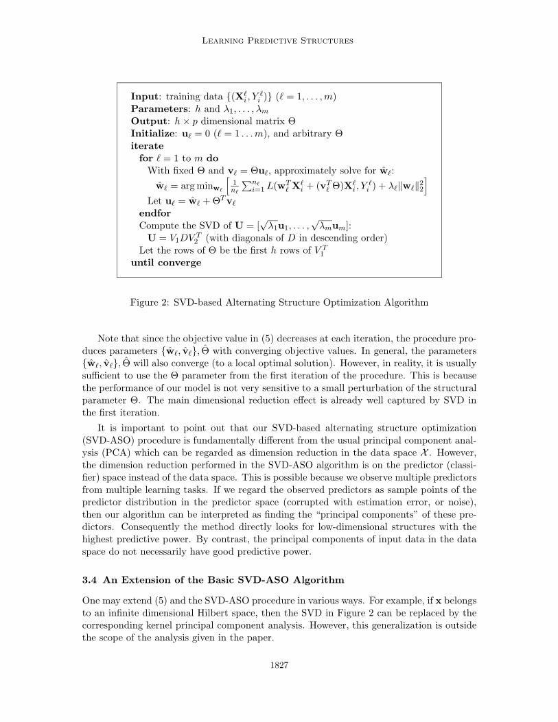
Learning Predictive Structures
Input: training data {(X`i , Y
`i )} (` = 1, . . . , m)
Parameters: h and λ1, . . . , λm
Output: h × p dimensional matrix ΘInitialize: u` = 0 (` = 1 . . . m), and arbitrary Θiterate
for ` = 1 to m doWith fixed Θ and v` = Θu`, approximately solve for w`:
w` = arg minw`
[
1n`
∑n`
i=1 L(wT` X`
i + (vT` Θ)X`
i , Y`i ) + λ`‖w`‖2
2
]
Let u` = w` + ΘTv`
endforCompute the SVD of U = [
√λ1u1, . . . ,
√λmum]:
U = V1DV T2 (with diagonals of D in descending order)
Let the rows of Θ be the first h rows of V T1
until converge
Figure 2: SVD-based Alternating Structure Optimization Algorithm
Note that since the objective value in (5) decreases at each iteration, the procedure pro-duces parameters {w`, v`}, Θ with converging objective values. In general, the parameters{w`, v`}, Θ will also converge (to a local optimal solution). However, in reality, it is usuallysufficient to use the Θ parameter from the first iteration of the procedure. This is becausethe performance of our model is not very sensitive to a small perturbation of the structuralparameter Θ. The main dimensional reduction effect is already well captured by SVD inthe first iteration.
It is important to point out that our SVD-based alternating structure optimization(SVD-ASO) procedure is fundamentally different from the usual principal component anal-ysis (PCA) which can be regarded as dimension reduction in the data space X . However,the dimension reduction performed in the SVD-ASO algorithm is on the predictor (classi-fier) space instead of the data space. This is possible because we observe multiple predictorsfrom multiple learning tasks. If we regard the observed predictors as sample points of thepredictor distribution in the predictor space (corrupted with estimation error, or noise),then our algorithm can be interpreted as finding the “principal components” of these pre-dictors. Consequently the method directly looks for low-dimensional structures with thehighest predictive power. By contrast, the principal components of input data in the dataspace do not necessarily have good predictive power.
3.4 An Extension of the Basic SVD-ASO Algorithm
One may extend (5) and the SVD-ASO procedure in various ways. For example, if x belongsto an infinite dimensional Hilbert space, then the SVD in Figure 2 can be replaced by thecorresponding kernel principal component analysis. However, this generalization is outsidethe scope of the analysis given in the paper.
1827
Ando and Zhang
In our experiments, we use another extension, where features (components of x) aregrouped into different types and the SVD dimension reduction is computed separately foreach group. This is important since in applications, features are not homogeneous. If weknow that some features are more similar to each other (e.g. they have the same type),then it is reasonable to perform a more localized dimension reduction among these similarfeatures. To formulate this idea, we divide input features into G groups, and rewrite eachinput data-point X`
i as [X`i,t]t=1,...,G, where t is the feature type which specifies which group
the feature is in. Each X`i,t ∈ Rpt , and thus X`
i ∈ Rp with p =∑G
t=1 pt. We associate
each group t with a structural parameter Θt ∈ Rht×pt , which is a projection operator ofthis feature type into ht dimensional space. Equation (5) can be replaced by the followingstructural learning method:
[{w`,t, v`,t}, {Θt}] = arg min{w`,t,v`,t}{Θt}
m∑
`=1
(
1
n`
n∑
i=1
L(G∑
t=1
(w`,t + ΘTt v`,t)
TX`i,t, Y
`i )
+
G∑
t=1
λ`,t‖w`,t‖22
)
, (8)
s.t. ∀t ∈ {1, . . . , G} : ΘtΘTt = Iht×ht
.
Similarly as before, we can introduce auxiliary variables u`,t = w`,t + ΘTt v`,t, and perform
alternating optimization over u and (Θ,v). The resulting algorithm is essentially the sameas the SVD-ASO method in Figure 2, but with the SVD dimension reduction step performedseparately for each feature group t.
Some other extensions of the basic algorithm can also be useful for certain applications.For example, we may choose to regularize only those components of w` which correspondto the non-negative part of u` (we may still regularize the negative part of u`, but using thecorresponding components of u` instead of w`). The reason for doing so is that the positiveweights of a linear classifier are usually directly related to the target concept, while thenegative components often yield much less specific information. The resulting method canbe easily formulated and solved by a variant of the basic SVD-ASO algorithm. In effect, inthe SVD computation, we only use the positive components of u`.
4. Semi-Supervised Learning
We are now ready to illustrate how to apply the structural learning paradigm developedearlier in the paper to the semi-supervised learning setting. The basic idea is to createauxiliary problems using unlabeled data, and then employ structural learning to revealpredictive structures intrinsic to the underlying input space X .
4.1 Learning from Unlabeled Data Through Structural Learning
We systematically create multiple prediction problems from unlabeled data. We call thesecreated prediction problems auxiliary problems, while we call the original supervised predic-tion problem (which we are interested in) the target problem.
Our method consists of the following two steps:
1828
Learning Predictive Structures
1. Learn a good structural parameter θ by performing a joint empirical risk minimizationon the auxiliary problems, using originally unlabeled data that are automatically‘labeled’ with auxiliary class labels.
2. Learn a predictor for the target problem by empirical risk minimization on the origi-nally labeled data, using θ computed in the first step. In particular, in our bi-linearformulation (Section 3), we fix Θ and optimize (8) with respect to w and v for thetarget problem.
The first step seeks a hypothesis space Hθ through learning the predictive functional struc-ture shared by auxiliary predictors. If auxiliary problems are, to some degree, related tothe target task, then the obtained hypothesis space Hθ, which improves the average perfor-mance of auxiliary predictors, will also help the target problem. Therefore, the relevancyof auxiliary problems plays an important role in our method. We will return to this issuein the next section.
An alternative to the above two-step procedure is to perform a joint empirical riskminimization on the target problem (with labeled data) and on the auxiliary problems (withunlabeled data) at once. However, in our intended applications, the number of labeled dataavailable for the target problem is usually small. Therefore the inclusion of the targetpredictor in the joint ERM will not have a significant impact.
4.2 Auxiliary Problem Creation
Our approach to semi-supervised learning requires auxiliary problems with the followingcharacteristics:
• Automatic labeling: we need to automatically generate various “labeled” data for theauxiliary problems from unlabeled data.
• Relevancy: auxiliary problems should be related to the target problem (that is, theyshare a certain predictive structure) to some degree.
We consider two strategies for automatic generation of auxiliary problems: one in a com-pletely unsupervised fashion, and the other in a partially supervised fashion. Some of theexample auxiliary problems introduced in this section are used in our experiments describedin Section 5.
We have briefly discussed the relationship of PCA and SVD-ASO in Section 3. In theabove mentioned framework of semi-supervised learning, the standard PCA (applied tounlabeled data) can also be roughly regarded as a result of generating k auxiliary problemsfrom k unlabeled data points so that the i-th problem has only one positive example (thei-th data point). In general, the strategies which we will suggest below are more flexibleand more effective.
For clarity, we introduce the following two mini target tasks as running examples.
Text genre categorization Consider the task of assigning one of the three categories in{ science, sports, economy } to text documents. For this problem, suppose that we usefrequencies of content words as features.
1829
Ando and Zhang
Word tagging Consider the task of assigning one of the three part-of-speech tags { noun,verb, other } to words in English sentences. For instance, the word “test” in “... a testprocedure ...” should be assigned the tag noun, and that in “We will test it ...” should beassigned the tag verb. For this problem, suppose that we use strings of the current andsurrounding words as features.
4.2.1 Unsupervised-Strategy: Predicting Observable Sub-structures
In the first strategy, we regard some observable substructures of the input data X as aux-iliary class labels, and try to predict these labels using other parts of the input data. Forinstance, for the word tagging task mentioned above, at each word position, we can createauxiliary problems by regarding the current word as auxiliary labels, which we want topredict using the surrounding words. We create one binary classification problem for eachpossible word value, and hence can obtain many auxiliary problems using this idea.
More generally, if we have a feature representation of the input data, then we may masksome features as unobserved, and learn classifiers to predict these ‘masked’ features (orsome functional mapping of the masked features, e.g., bi-grams of left and current words)based on other features that are not masked. In the actual implementation, we just replacethe masked feature values by zero, which has the same effect.
The automatic-labeling requirement is satisfied since the auxiliary labels are observableto us. To see why this technique may naturally meet the relevancy requirement, we notethat feature components that can predict a certain masked feature are correlated to themasked feature, and thus are correlated among themselves. Therefore this technique helpsus to identify correlated features with predictive power.
However, for optimal performance, it is clear that we should choose to mask (and pre-dict) features that have good correlation to the target classes as auxiliary labels. Thecreation of auxiliary problems following this strategy is thus as easy or hard as designingfeatures for usual supervised learning tasks. We can often make an educated guess basedon task-specific knowledge. A wrong guess would result in adding some irrelevant features(originating from irrelevant θ-components), but it would not hurt ERM learners severely.On the other hand, potential gains from a right guess can be significant. Also note thatgiven the abundance of unlabeled data, we have a wider range of choices than standardfeature engineering in the supervised setting. For example, high-order features that sufferfrom the data sparseness problem in the supervised setting may be used in auxiliary prob-lems due to the vast amount of unlabeled data that can provide more reliable statistics.The low-dimensional predictive structure discovered from the high-order features can thenbe used in the supervised task without causing the data-sparseness problem. This is be-cause the rare features will be properly combined in the projection matrix Θ, so that thecombined low-dimension directions will appear more frequently (and more correlated to theclass-label). The example provided in Section 4.3 demonstrates this point.
The following examples illustrate auxiliary problems potentially useful for our examplemini tasks.
Ex 1. Predict frequent words for text genre categorization. It is intuitive thatcontent words that occur frequently in a document are often good indicators of the genreof that document. Let us split content words into two sets W1 and W2 (after removing
1830
Learning Predictive Structures
appropriate stop words). An auxiliary task we define is as follows. Given document x,predict the word that occurs most frequently in x, among the words in set W1. The learneronly uses the words in W2 for this prediction. This task breaks down to |W1| binaryprediction problems, one for each content word in W1.
1
For example, let
W1 = {“stadium”, “scientist”, “stock”} ,
W2 = {“baseball”, “basketball”, “physics”, “market”} .
We treat members of W1 as unobserved, and learn to predict whether the word “stadium”occurs more frequently in a document than “scientist” and “stock” by observing the occur-rences of “baseball”, “basketball”, “physics”, and “market”. Similarly, the second problemis to predict whether “scientist” is more frequent than “baseball” and “stock”. Essentially,through this auxiliary problem, we learn the textual context in W2 that implies that theword “stadium” occurs frequently in W1. Assuming that “stadium” is a strong indicator ofsports, the problem indirectly helps to learn the correlation of W2 members to the targetclass sports from unlabeled data.
Ex 2. Predict word strings for word tagging. As we have already discussed above,an example auxiliary task for word tagging is to predict the word string at the currentposition by observing the corresponding words on the left and the right. Using this idea,we can obtain |W | binary prediction problems where W is a set of all possible word strings.Another example is to predict the word on the left by observing the words at the currentand right positions. The underlying assumption is that word strings (at the current andleft positions) have strong correlations to the target problem – whether a word is noun orverb.
4.2.2 Partially Supervised-Strategy: Predicting the Behavior of TargetClassifier
The second strategy is motivated by co-training. We use two (or more) distinct featuremaps: Φ1 : X → F and Φ2 : X → F . First, we train a classifier for the target task, usingthe feature map Φ1 and the labeled data. The auxiliary tasks are to predict the behavior ofthis classifier (such as predicted labels, assigned confidence values, and so forth), by usingthe other feature map Φ2. Note that unlike co-training, we only use the classifier as ameans of creating auxiliary problems that meet the relevancy requirement, instead of usingit to bootstrap labels. The semi-supervised learning procedure following this strategy issummarized as follows.
1. Train a classifier T1 with labeled data Z for the target task, using feature map Φ1.
2. Generate labeled data for auxiliary problems by applying T1 to unlabeled data.
3. Learn structural parameter θ by performing joint ERM on the auxiliary problems,using only the feature map Φ2.
1. One may also consider variations of this idea, such as predicting whether a content word in W1 appearsmore often than a certain threshold, or in the top-k most frequent list of x.
1831
Ando and Zhang
4. Train a final classifier with labeled data Z, using θ computed above and some appro-priate feature map Ψ.
Ex 3. Predict the prediction of classifier T1. The simplest auxiliary task created byfollowing this strategy is the prediction of the class labels proposed by classifier T1. Whenthe target task is c-way classification, c binary classification problems are obtained in thismanner. For example, suppose that we train a classifier using only one half of content wordsfor the text genre categorization task. Then, one of auxiliary problems will be to predictwhether this classifier would propose sports category or not, based on the other half ofcontent words only.
Ex 4. Predict the top-k choices of the classifier. Another example is to predictthe combinations of k (a few) classes to which T1 assigns the highest confidence values.Through this problem, fine-grained distinctions (related to intrinsic sub-classes of targetclasses) can be learned. From a c-way classification problem, c!/(c − k)! binary predictionproblems can be created. For instance, predict whether T1 assigns the highest confidencevalues to sports and economy in this order.
Ex 5. Predict the range of confidence values produced by the classifier. Yetanother example is to predict the proposed labels in conjunction with the range of confidencevalues. For instance, predict whether T1 would propose sports with confidence greater than0.5.
4.3 Discussions
We have introduced two strategies for creating auxiliary problems in this section. One isunsupervised, and the other partially supervised.
For the unsupervised strategy, we try to predict some sub-structures of the input usingsome other parts of the input. This idea is related to the discussion in Section 2.3, wherewe have argued that there are often good structures (or smoothness conditions) intrinsicto the input space. These structures can be discovered from auxiliary problems. For textdata, some words or linguistic usages will have similar meanings. The smoothness conditionis related to the fact that interesting predictors for text data (often associated with someunderlying semantic meanings) will take similar values when a linguistic usage is substitutedby one that is closely related. This smoothness structure can be discovered using structurallearning, and specifically by the method we proposed in Section 3. In this case, the spaceof smooth predictors corresponds to the most predictive low dimensional directions whichwe may discover using the SVD-ASO algorithm. An example of computed Θ is given inSection 5.2.8, which supports the argument. It is also easy to see that this reasoning isnot specific to text. Therefore the idea can be applied to other data such as images. Inthe following, we will briefly explain the underlying intuition on why the un-supervisedauxiliary problems we create are helpful for the supervised task, and leave the developmentof a more rigorous and general theory to future investigation.
Suppose we split the features into two parts W1 and W2, and then predict W1 based onW2. Suppose features in W1 are correlated to the class labels (but not necessarily correlatedamong themselves). Then, the auxiliary prediction problems are related to the target task,and thus can reveal useful structures of W2. Under appropriate conditions, features in W2
1832
Learning Predictive Structures
with similar predictive performance tend to map to similar low-dimensional vectors throughΘ. This effect can be empirically observed in Section 5.2.8. We shall only use a simple butconcrete example to illustrate the main idea. Assume that words are divided into fivedisjoint sets Tj : −2 ≤ j ≤ 2 , with binary label y ∈ {−1, 1}. Assume also for simplicitythat every document contains only two words x1 and x2, where x1 ∈ W1 = ∪j=−1,0,1Tj ,and x2 ∈ W2 = ∪j=−2,2Tj . Assume further that given class label y = ±1, x1 and x2 areindependent, where x1 is uniformly distributed over T0 ∪Ty and x2 is uniformly distributedover T2y. Then by predicting x1 = ` based on x2 with least squares, we obtain for eachy ∈ {±1}, identical weight-components for all words in T2y (due to the exchangeability ofwords in each T2y). Thus after dimension reduction, only two rows of Θ have non-zerosingular values. The Θ-feature reduces all words in T2 to a single vector in R2, and allwords in T−2 into another single vector in R2. This gives a helpful grouping effect (wordswith similar predictive performance are grouped together). It is clear that in this example,we gain predictive ability by using unsupervised structure discovery. This is because theoriginal word-spaces T2 and T−2 may be extremely large, which means that one will not beable to learn very well from a small number of training examples (since each word does notoccur often enough). By grouping all words in T2 (also in T−2) together, we obtain a featurethat is completely correlated to the class label due to our data generation process. Thereforethe grouping effect makes the originally hard problem much easier to learn. This examplecan be extended to a more general theory, which we shall leave to further exploration. Theconsequence of the example is observable in practice, as demonstrated in Section 5.2.8.
Although the above discussion implies that it is possible to find useful predictive struc-tures even if we do not intentionally create problems to mimic the target problem, it isalso clear that auxiliary problems more closely related to the target problem will be morebeneficial. This is our motivation to propose the partially supervised strategy for creatingauxiliary problems. Using this idea, it is always possible to create relevant auxiliary prob-lems that are closely related to the supervised problem without knowing the effectivenessof the individual features. In practical applications, we observe that it can be desirable tocreate as many auxiliary problems as possible, as long as there is some reason to believein their relevancy to the target task. This is because the risk is relatively minor, while thepotential gain from a good structure is large.
Moreover, the auxiliary problems introduced above (and used in our experiments ofthe next section) are merely possible examples. One advantage of this approach to semi-supervised learning is that one may design a wide variety of auxiliary problems for learningvarious aspects of the target problem from unlabeled data. Structural learning provides atheoretical foundation and a general framework for carrying out possible new ideas.
5. Experiments
We study the performance of our structural learning-based semi-supervised method on textcategorization, natural language tagging/chunking, and image classification tasks. Theexperimental results show that we are able to improve state-of-the-art supervised learningmethods even for some problems with relatively large number of labeled data (e.g. 200Klabeled data for named entity recognition).
1833
Ando and Zhang
5.1 Implementation
We experiment with the following semi-supervised learning procedure:
1. If required for auxiliary label generation, train classifiers Ti using labeled data Z andappropriate feature maps Ψi.
2. For all the auxiliary problems, assign auxiliary labels to unlabeled data.
3. Compute structure matrix Θ by performing the SVD-ASO procedure (Section 3) usingall auxiliary problems on the data generated above. We use the extended version totake advantage of natural feature splits, and iterate once.
4. Fix Θ and obtain the final classifier by optimizing (8) with respect to w and v, usinglabeled data Z.
In all settings (including baseline methods), the loss function is a modification of theHuber’s robust loss for regression:
L(p, y) =
{
max(0, 1 − py)2 if py ≥ −1−4py otherwise
,
with square regularization (λ = 10−4). It is known that the modified Huber loss works wellfor classification, and has some advantages, although one may select other loss functionssuch as SVM or logistic regression. The specific choice is not important for the purposeof this paper. The training algorithm is stochastic gradient descent (SGD) as in (Zhang,2004). We fix ht (dimension of Θt) to 50, and use it for all the settings unless otherwisespecified.
5.2 Text Categorization Experiments
We report text categorization performance on the 20-newsgroup corpus and the Reuters-RCV1 corpus (also known as “new Reuters”).
5.2.1 Feature Representation
Our feature representation uses word frequencies after removing function words and commonstopwords, and normalizes feature vectors into unit vectors.
5.2.2 Auxiliary Problems for Text Categorization
We experiment with the following types of auxiliary problems:
• Freq: predicts the most frequent word by observing one half of the words (as in Section4.2.1. Ex 1).
• Top-k: predicts combinations of the top-k choices of the classifier trained with labeleddata (as in Section 4.2.2. Ex 4).
• Multi-k: for the multi-category target task, predicts the top-k choices of the classifier(trained with labeled data), regarding them as multi-category auxiliary labels. The
1834
Learning Predictive Structures
number k is set to the average number of categories per instance, obtained from thelabeled data.
Feature splits are randomly generated.
5.2.3 Data
20-newsgroup corpus The 20-newsgroup corpus is one of the standard data sets for textcategorization, which consists of 20K documents from 20 newsgroups, with 1K documentsper group. The task is to classify documents into these 20 newsgroups ranging over a varietyof topics – computer hardware, baseball, bikes, religions, middle east issues, and so on. Inpre-processing, we removed the header lines (subjects, newsgroup names, senders, and soforth) from all documents. We held out 1K documents as the test set, and arbitrarily splitthe rest of the corpus into the training set (2K documents) and the unlabeled data set (17Kdocuments).
Reuters-RCV1 corpus (new Reuters) From the Reuters-RCV1 corpus, we randomlygenerate disjoint sets of labeled (1K), unlabeled (20K), and test (3K) examples. TheReuters-RCV1 corpus differs from the 20-newsgroup corpus in several ways. The num-ber of categories is 102, which is five times larger than that of the 20-newsgroup corpus;the categories are organized into three-level hierarchies; each document may be assignedmultiple categories — about three categories per document on average. The Reuters-RCV1corpus preserves the natural distribution of the categories whereas the 20-newsgroup corpushas a completely uniform distribution, generated by intentionally choosing the same numberof documents from each newsgroup.
5.2.4 Evaluation Metric
To measure the performance of the final classifier on the test sets, for singly-labeled tasks,we choose one category that produces the highest confidence value (inner product) andreport classification accuracy. For multiply-labeled tasks, we choose categories that producepositive confidence values, and report the micro-averaged F-measure.
5.2.5 Text Categorization Performance Results
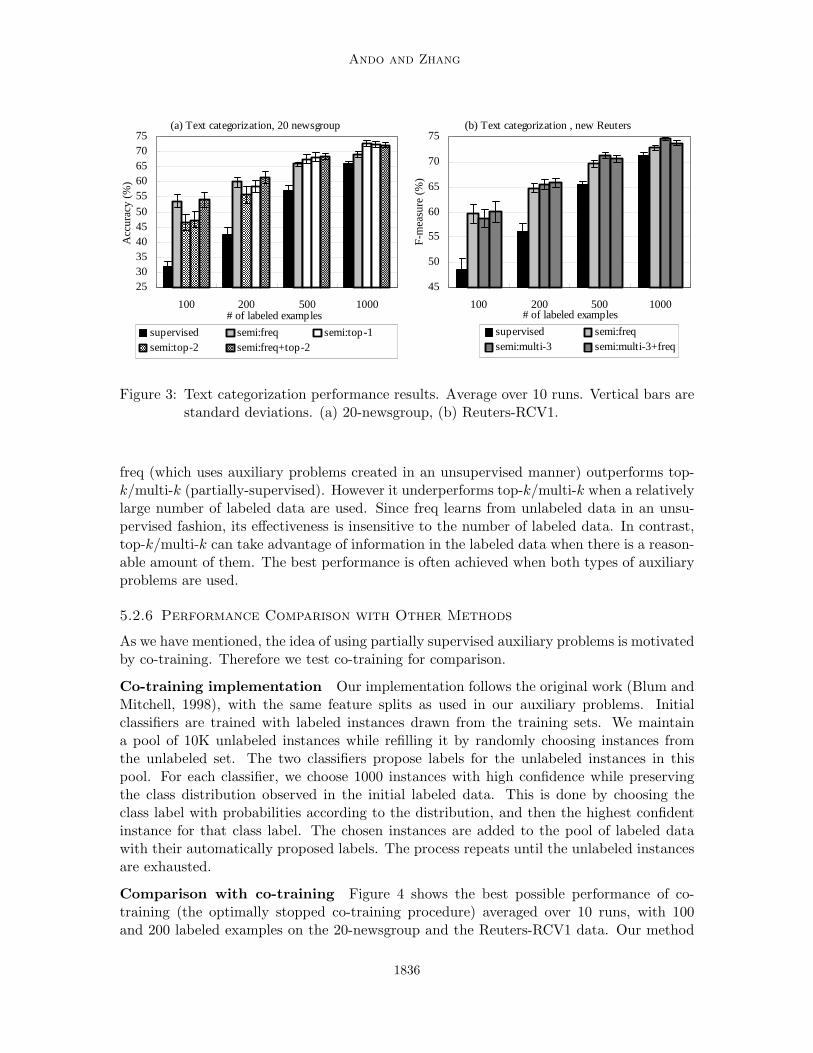
20-newsgroup results Figure 3 (a) shows the accuracy results on the 20-newsgroup datain comparison with the supervised setting as the baseline. We show the averaged results over10 runs, each with labeled examples randomly drawn from the training set. The verticalbars are ‘one’ standard deviations. The symbol ‘semi’ stands for semi-supervised, followedby the types of auxiliary problems used. The semi-supervised methods obtain significantperformance improvements (up to 22.2%) over the supervised method in all settings.
Reuters-RCV1 results Figure 3 (b) shows micro-averaged F-measure on the Reuters-RCV1 data in comparison to the supervised baseline. The performance trend is similarto that of the 20-newsgroup experiments. Significant performance improvements (up to11.6%) over the supervised method are obtained in all settings.
Auxiliary problems: unsupervised vs. partially-supervised From the resultsin Figure 3, we observe that when a relatively small number of labeled data are used,
1835
Ando and Zhang
(a) Text categorization, 20 newsgroup
253035404550
5560657075
100 200 500 1000# of labeled examples
Acc
urac
y (%
)
supervised semi:freq semi:top-1semi:top-2 semi:freq+top-2
(b) Text categorization , new Reuters
45
50
55
60
65
70
75
100 200 500 1000# of labeled examples
F-m
easu
re (
%)
supervised semi:freqsemi:multi-3 semi:multi-3+freq
Figure 3: Text categorization performance results. Average over 10 runs. Vertical bars arestandard deviations. (a) 20-newsgroup, (b) Reuters-RCV1.
freq (which uses auxiliary problems created in an unsupervised manner) outperforms top-k/multi-k (partially-supervised). However it underperforms top-k/multi-k when a relativelylarge number of labeled data are used. Since freq learns from unlabeled data in an unsu-pervised fashion, its effectiveness is insensitive to the number of labeled data. In contrast,top-k/multi-k can take advantage of information in the labeled data when there is a reason-able amount of them. The best performance is often achieved when both types of auxiliaryproblems are used.
5.2.6 Performance Comparison with Other Methods
As we have mentioned, the idea of using partially supervised auxiliary problems is motivatedby co-training. Therefore we test co-training for comparison.
Co-training implementation Our implementation follows the original work (Blum andMitchell, 1998), with the same feature splits as used in our auxiliary problems. Initialclassifiers are trained with labeled instances drawn from the training sets. We maintaina pool of 10K unlabeled instances while refilling it by randomly choosing instances fromthe unlabeled set. The two classifiers propose labels for the unlabeled instances in thispool. For each classifier, we choose 1000 instances with high confidence while preservingthe class distribution observed in the initial labeled data. This is done by choosing theclass label with probabilities according to the distribution, and then the highest confidentinstance for that class label. The chosen instances are added to the pool of labeled datawith their automatically proposed labels. The process repeats until the unlabeled instancesare exhausted.
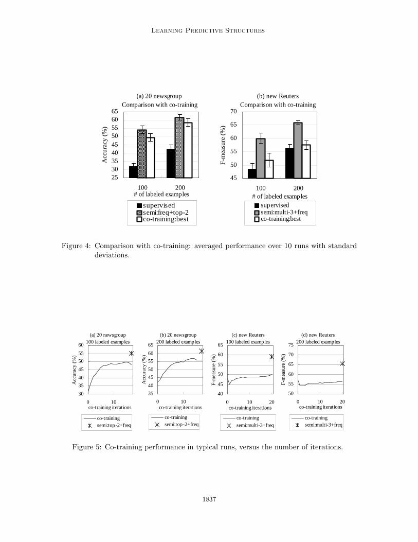
Comparison with co-training Figure 4 shows the best possible performance of co-training (the optimally stopped co-training procedure) averaged over 10 runs, with 100and 200 labeled examples on the 20-newsgroup and the Reuters-RCV1 data. Our method
1836
Learning Predictive Structures
(a) 20 newsgroupComparison with co-training
253035404550556065
100 200# of labeled examples
Acc
urac
y (%
)
supervisedsemi:freq+top-2co-training:best
(b) new ReutersComparison with co-training
45
50
55
60
65
70
100 200# of labeled examples
F-m
easu
re (
%)
supervisedsemi:multi-3+freqco-training:best
Figure 4: Comparison with co-training: averaged performance over 10 runs with standarddeviations.
(a) 20 newsgroup100 labeled examples
30
35
40
45
50
55
60
0 10co-training iterations
Acc
urac
y (%
)
co-trainingsemi:top-2+freq
(b) 20 newsgroup200 labeled examples
35
40
45
50
55
60
65
0 10co-training iterations
Acc
urac
y (%
)
co-trainingsemi:top-2+freq
(c) new Reuters100 labeled examples
40
45
50
55
60
65
0 10 20co-training iterations
F-m
easu
re (
%)
co-training
semi:multi-3+freq
(d) new Reuters200 labeled examples
50
55
60
65
70
75
0 10 20co-training iterations
F-m
easu
re (
%)
co-trainingsemi:multi-3+freq
Figure 5: Co-training performance in typical runs, versus the number of iterations.
1837
Ando and Zhang
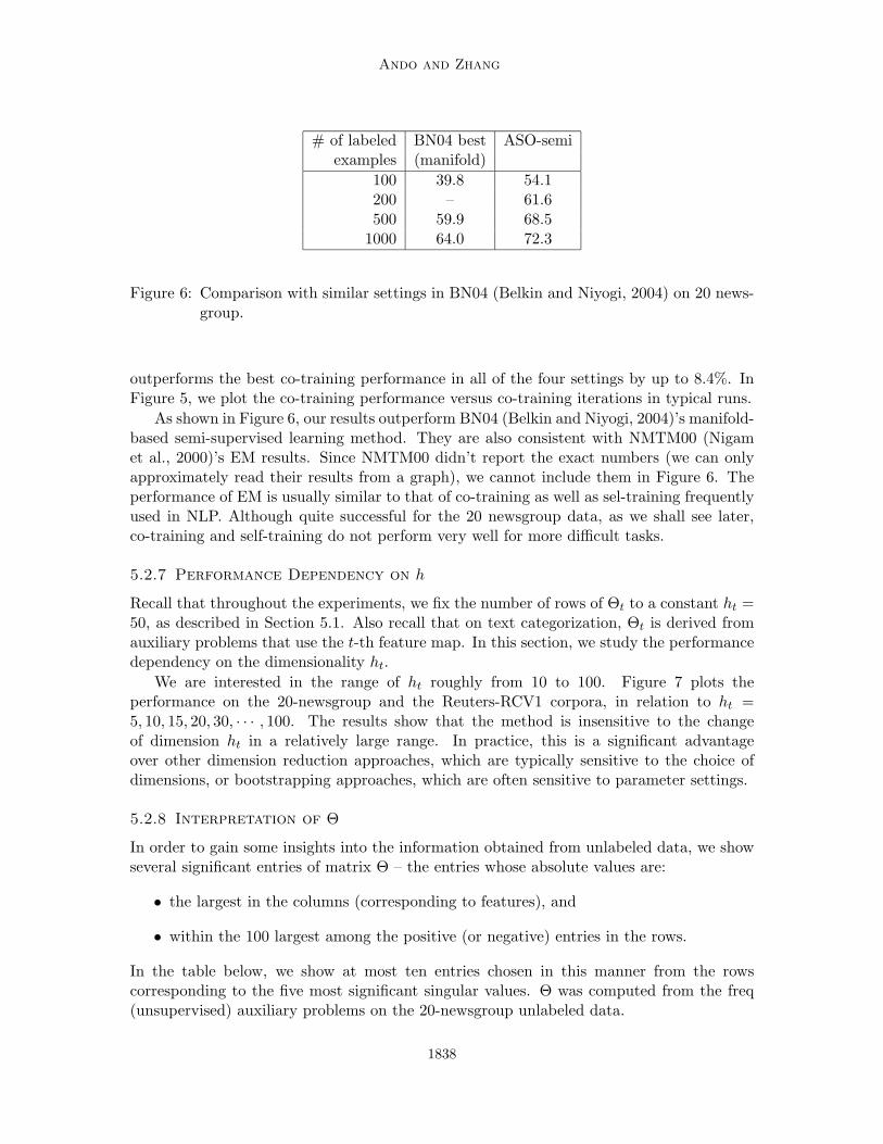
# of labeled BN04 best ASO-semiexamples (manifold)
100 39.8 54.1200 – 61.6500 59.9 68.5
1000 64.0 72.3
Figure 6: Comparison with similar settings in BN04 (Belkin and Niyogi, 2004) on 20 news-group.
outperforms the best co-training performance in all of the four settings by up to 8.4%. InFigure 5, we plot the co-training performance versus co-training iterations in typical runs.
As shown in Figure 6, our results outperform BN04 (Belkin and Niyogi, 2004)’s manifold-based semi-supervised learning method. They are also consistent with NMTM00 (Nigamet al., 2000)’s EM results. Since NMTM00 didn’t report the exact numbers (we can onlyapproximately read their results from a graph), we cannot include them in Figure 6. Theperformance of EM is usually similar to that of co-training as well as sel-training frequentlyused in NLP. Although quite successful for the 20 newsgroup data, as we shall see later,co-training and self-training do not perform very well for more difficult tasks.
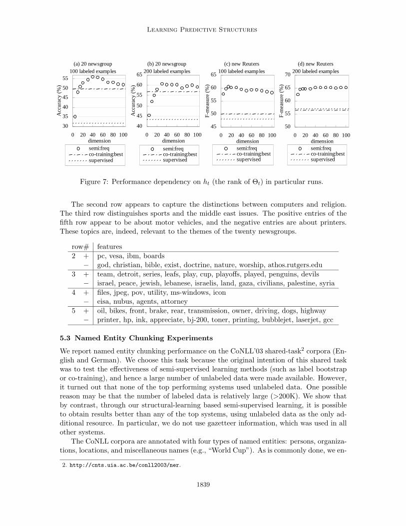
5.2.7 Performance Dependency on h
Recall that throughout the experiments, we fix the number of rows of Θt to a constant ht =50, as described in Section 5.1. Also recall that on text categorization, Θt is derived fromauxiliary problems that use the t-th feature map. In this section, we study the performancedependency on the dimensionality ht.
We are interested in the range of ht roughly from 10 to 100. Figure 7 plots theperformance on the 20-newsgroup and the Reuters-RCV1 corpora, in relation to ht =5, 10, 15, 20, 30, · · · , 100. The results show that the method is insensitive to the changeof dimension ht in a relatively large range. In practice, this is a significant advantageover other dimension reduction approaches, which are typically sensitive to the choice ofdimensions, or bootstrapping approaches, which are often sensitive to parameter settings.
5.2.8 Interpretation of Θ
In order to gain some insights into the information obtained from unlabeled data, we showseveral significant entries of matrix Θ – the entries whose absolute values are:
• the largest in the columns (corresponding to features), and
• within the 100 largest among the positive (or negative) entries in the rows.
In the table below, we show at most ten entries chosen in this manner from the rowscorresponding to the five most significant singular values. Θ was computed from the freq(unsupervised) auxiliary problems on the 20-newsgroup unlabeled data.
1838
Learning Predictive Structures
(a) 20 newsgroup100 labeled examples
30
35
40
45
50
55
0 20 40 60 80 100dimension
Acc
urac
y (%
)
semi:freqco-training:bestsupervised
(d) new Reuters200 labeled examples
50
55
60
65
70
0 20 40 60 80 100dimension
F-m
easu
re (
%)
semi:freqco-training:bestsupervised
(b) 20 newsgroup200 labeled examples
40
45
50
55
60
65
0 20 40 60 80 100dimension
Acc
urac
y (%
)
semi:freqco-training:bestsupervised
(c) new Reuters100 labeled examples
45
50
55
60
65
0 20 40 60 80 100dimension
F-m
easu
re (
%)
semi:freqco-training:bestsupervised
Figure 7: Performance dependency on ht (the rank of Θt) in particular runs.
The second row appears to capture the distinctions between computers and religion.The third row distinguishes sports and the middle east issues. The positive entries of thefifth row appear to be about motor vehicles, and the negative entries are about printers.These topics are, indeed, relevant to the themes of the twenty newsgroups.
row# features
2 + pc, vesa, ibm, boards− god, christian, bible, exist, doctrine, nature, worship, athos.rutgers.edu
3 + team, detroit, series, leafs, play, cup, playoffs, played, penguins, devils− israel, peace, jewish, lebanese, israelis, land, gaza, civilians, palestine, syria
4 + files, jpeg, pov, utility, ms-windows, icon− eisa, nubus, agents, attorney
5 + oil, bikes, front, brake, rear, transmission, owner, driving, dogs, highway− printer, hp, ink, appreciate, bj-200, toner, printing, bubblejet, laserjet, gcc
5.3 Named Entity Chunking Experiments
We report named entity chunking performance on the CoNLL’03 shared-task2 corpora (En-glish and German). We choose this task because the original intention of this shared taskwas to test the effectiveness of semi-supervised learning methods (such as label bootstrapor co-training), and hence a large number of unlabeled data were made available. However,it turned out that none of the top performing systems used unlabeled data. One possiblereason may be that the number of labeled data is relatively large (>200K). We show thatby contrast, through our structural-learning based semi-supervised learning, it is possibleto obtain results better than any of the top systems, using unlabeled data as the only ad-ditional resource. In particular, we do not use gazetteer information, which was used in allother systems.
The CoNLL corpora are annotated with four types of named entities: persons, organiza-tions, locations, and miscellaneous names (e.g., “World Cup”). As is commonly done, we en-
2. http://cnts.uia.ac.be/conll2003/ner.
1839
Ando and Zhang
code chunk information into word tags to cast the chunking problem to that of word tagging,and perform Viterbi-style decoding. We use the official training/development/test splits, asprovided by the shared-task organizers. Our unlabeled data sets consist of 27 million words(English) and 35 million words (German), respectively. They were chosen from the samesources – Reuters and ECI Multilingual Text Corpus – as the training/development/testsets but disjoint from them.
5.3.1 Feature Representation
Our feature representation is a slight modification of a simpler configuration reported in(Zhang and Johnson, 2003), which uses: token strings, parts-of-speech, character types,several characters at the beginning and the ending of the tokens, in a 5-token windowaround the current position; token strings in a 3-syntactic chunk window; labels of twotokens on the left to the current position; bi-grams of the current token and the label onthe left; and the labels assigned to previous occurrences of the current word. These featuresare easily obtained without deep linguistic processing.
5.3.2 Auxiliary Problems for Named Entity Chunking
We use four types of auxiliary problems and their combinations:
• Word prediction: predicts the word at the current (or left or right) position, using thefeatures derived from the other tokens.
• Top-2: predicts the top-2 choices of the classifier. We split features into “left-contextvs. the others” and “right-context vs. the others”. The rest is the same as Ex 4 inSection 4.2.2.
SVD is applied to each of the feature types separately. As for the word-prediction auxiliaryproblems, we only consider the instances whose current words are either nouns or adjectivessince named entities mostly consist of these types. Also, we leave out all but 1000 auxiliaryproblems of each type that have the largest numbers of positive examples. This is to ensurethat auxiliary predictors can be adequately learned from unlabeled data.
5.3.3 Performance Results on the CoNLL English/German Corpora
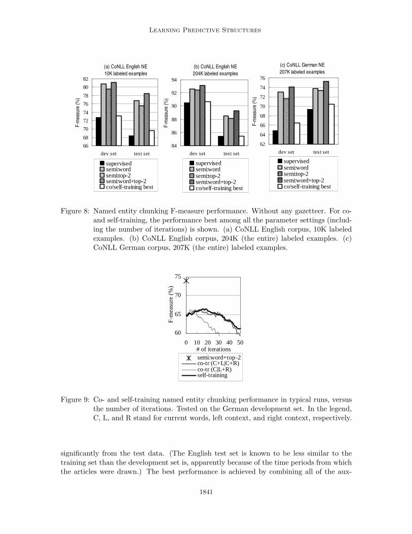
Figures 8 (a) and (b) show the English F-measure results – (a) with small (10K-word)labeled data, and (b) with the entire training set (204K words). German results using theentire training set are shown in Figure 8 (c). Precision and recall results in the same settingsare found in Figure 15.
Note that to facilitate comparisons with the supervised baselines, we do not use anygazetteers or any name lexicons. Thus, there are only two kinds of information sources:labeled data and unlabeled data. We confirm that performance improvements gained byunlabeled data are significant in all of the semi-supervised settings: up to 10.10% gainswith small English labeled data, up to 3.86% with larger English labeled data, and up to9.22% improvements on the German data.
We note that word-prediction (unsupervised) auxiliary problems are particularly effec-tive when the number of labeled examples is relatively small or the training data differ
1840
Learning Predictive Structures
(a) CoNLL English NE
10K labeled examples
66
68
70
72
74
76
78
80
82
dev set test set
F-m
easu
re (
%)
supervisedsemi:wordsemi:top-2semi:word+top-2co/self-training best
(b) CoNLL English NE
204K labeled examples
84
86
88
90
92
94
dev set test set
F-m
easu
re (
%)
supervisedsemi:wordsemi:top-2semi:word+top-2co/self-training best
(c) CoNLL German NE
207K labeled examples
62
64
66
68
70
72
74
76
dev set test set
F-m
easu
re (
%)
supervisedsemi:wordsemi:top-2semi:word+top-2co/self-training best
Figure 8: Named entity chunking F-measure performance. Without any gazetteer. For co-and self-training, the performance best among all the parameter settings (includ-ing the number of iterations) is shown. (a) CoNLL English corpus, 10K labeledexamples. (b) CoNLL English corpus, 204K (the entire) labeled examples. (c)CoNLL German corpus, 207K (the entire) labeled examples.
60
65
70
75
0 10 20 30 40 50# of iterations
F-m
easu
re (
%)
semi:word+top-2co-tr (C+L|C+R)co-tr (C|L+R)self-training
Figure 9: Co- and self-training named entity chunking performance in typical runs, versusthe number of iterations. Tested on the German development set. In the legend,C, L, and R stand for current words, left context, and right context, respectively.
significantly from the test data. (The English test set is known to be less similar to thetraining set than the development set is, apparently because of the time periods from whichthe articles were drawn.) The best performance is achieved by combining all of the aux-
1841
Ando and Zhang
iliary problems. This performance trend is in line with that in the text categorizationexperiments.
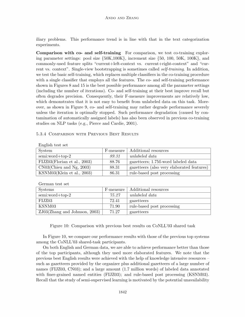
Comparison with co- and self-training For comparison, we test co-training explor-ing parameter settings: pool size {50K,100K}, increment size {50, 100, 50K, 100K}, andcommonly-used feature splits “current+left-context vs. current+right-context” and “cur-rent vs. context”. Single-view bootstrapping is sometimes called self-training. In addition,we test the basic self-training, which replaces multiple classifiers in the co-training procedurewith a single classifier that employs all the features. The co- and self-training performanceshown in Figures 8 and 15 is the best possible performance among all the parameter settings(including the number of iterations). Co- and self-training at their best improve recall butoften degrades precision. Consequently, their F-measure improvements are relatively low,which demonstrates that it is not easy to benefit from unlabeled data on this task. More-over, as shown in Figure 9, co- and self-training may rather degrade performance severelyunless the iteration is optimally stopped. Such performance degradation (caused by con-tamination of automatically assigned labels) has also been observed in previous co-trainingstudies on NLP tasks (e.g., Pierce and Cardie, 2001).
5.3.4 Comparison with Previous Best Results
English test set
System F-measure Additional resources
semi:word+top-2 89.31 unlabeled data
FIJZ03(Florian et al., 2003) 88.76 gazetteers; 1.7M-word labeled data
CN03(Chieu and Ng, 2003) 88.31 gazetteers (also very elaborated features)
KSNM03(Klein et al., 2003) 86.31 rule-based post processing
German test set
Systems F-measure Additional resources
semi:word+top-2 75.27 unlabeled data
FIJZ03 72.41 gazetteers
KSNM03 71.90 rule-based post processing
ZJ03(Zhang and Johnson, 2003) 71.27 gazetteers
Figure 10: Comparison with previous best results on CoNLL’03 shared task
In Figure 10, we compare our performance results with those of the previous top systemsamong the CoNLL’03 shared-task participants.
On both English and German data, we are able to achieve performance better than thoseof the top participants, although they used more elaborated features. We note that theprevious best English results were achieved with the help of knowledge intensive resources –such as gazetteers provided by the organizer plus additional gazetteers of a large number ofnames (FIJZ03, CN03); and a large amount (1.7 million words) of labeled data annotatedwith finer-grained named entities (FIJZ03); and rule-based post processing (KSNM03).Recall that the study of semi-supervised learning is motivated by the potential unavailability
1842
Learning Predictive Structures
of such labor intensive resources. Hence, we feel that our results, which were obtained byusing unlabeled data as the only additional resource, are very encouraging.
5.4 Part-of-Speech Tagging
We report part-of-speech (POS) tagging results on the Brown corpus. This corpus, anno-tated with 46 parts-of-speech, is one of the standard corpora for POS tagging research. Wearbitrarily split the corpus into the labeled set (23K words), unlabeled set (1M words), andthe test set (60K words).
The same auxiliary problems and feature representation (as in the named entity chunkingexperiments) are used, except for part-of-speech and syntactic chunk information. Followingthe convention, we use error rate to measure the performance. It can be seen from Figure11 that over 20% error reductions are achieved by learning from unlabeled data.
supervised 8.9
semi:left+curr 7.0 (21.3%)semi:top-1 6.9 (22.5%)semi:left+curr+top-1 6.9 (22.5%)
Figure 11: Part-of-speech tagging error rates (%). The numbers in parentheses are errorreduction ratio with respect to the supervised baseline.
5.5 Hand-Written Digit Image Classification
This experiment uses the MNIST data downloaded from http://yann.lecun.com/exdb/mnist/.It consists of a training set (60K examples) and a test set (10K examples) of 28-by-28 gray-scale hand-written digits. The task is to classify the image data into 10 digits,‘0’– ‘9’.
We use a feature representation composed of location-sensitive bags of pixel blocks,similar to the bag-of-word model in text categorization. It consists of normalized counts ofpixel blocks of various shapes in the four regions (top-left, top-right, bottom-right, bottom-left). (Normalization was done by scaling the vector for each shape/region into a unitvector.) The pixel blocks are black-white patterns of 16 pixels in the shape of: squares(4×4),rectangles(2 × 8, 8 × 2), crossing lines (from top-left to bottom-right; from top-right tobottom-left), and dotted lines (horizontal and vertical). Using these features and trainedwith the entire training set (60K examples), the error rate in the supervised setting is0.82%. This matches/surpasses state-of-the-art algorithms on the same data (reported onthe MNIST data website) without additional image processing or transformation such asdistortion or deskewing.
Auxiliary problems we used are partially-supervised. Feature splits were made by halv-ing each image: features derived from top-left+top-right regions vs. those from bottom-left+bottom-right; top-left+bottom-left vs. top-right+bottom-right; and top-left+bottom-right vs. top-right+bottom-left.
In each run, labeled examples were randomly chosen from the training set, with theremaining training set used as unlabeled data. ASO-semi (Figure 12) consistently produced
1843
Ando and Zhang
significant performance improvements over the supervised baseline.3 It also outperformsa manifold-based semi-supervised learning method BN04 (Belkin and Niyogi, 2004) exceptwhen the number of labeled data is 100. The method in BN04 performs well for smalllabeled data. However, a disadvantage is that their method (which also requires dimensionreduction) is more sensitive to the number of reduced dimensions. For example, with 100labeled data, they achieved an error rate of 6.4 with 20 dimensions, but an error rate of22.0 with 10 dimensions, and an error rate of 14.4 with 50 dimensions.
#labeled supervised ASO-semi BN04 best (2nd best)
100 14.22 ± 2.90 9.13 ± 1.95 6.4 (14.4)500 3.93 ± 0.22 3.05 ± 0.20 3.5 (3.6)
1000 2.83 ± 0.16 2.26 ± 0.11 3.2 (3.4)5000 1.64 ± 0.07 1.47 ± 0.07 2.7 (2.9)
Figure 12: Error rates (%); average over 10 runs and standard deviation. MNIST hand-writtendigit image classification results on the test set. BN04 results (Belkin and Niyogi, 2004)are on the unlabeled portion of the training set.
(a) 20-newsgroup# of labeled examples 100 200 500 1000
supervised 32.0 42.7 56.9 66.0semi:freq 53.6 (+21.6) 60.0 (+17.3) 65.8 (+8.9) 69.1 (+3.1)semi:top-1 46.6 (+14.6) 55.9 (+13.2) 67.6 (+10.7) 72.9 (+6.9)semi:top-2 47.4 (+15.4) 58.4 (+15.7) 68.3 (+11.4) 72.5 (+6.5)semi:top-2+freq 54.1 (+22.1) 61.6 (+18.9) 68.5 (+11.6) 72.3 (+6.3)
(b) Reuters-RCV1 corpus# of labeled examples 100 200 500 1000
supervised 48.5 56.3 65.4 71.4semi:freq 59.6 (+11.1) 64.8 (+8.5) 69.6 (+4.2) 72.8 (+1.4)semi:multi-3 58.7 (+10.2) 65.5 (+9.2) 71.2 (+5.8) 74.6 (+3.2)semi:multi-3+freq 60.1 (+11.6) 65.8 (+9.5) 70.7 (+5.3) 73.7 (+2.3)
Figure 13: Text categorization. Average over 10 runs. For each run, labeled exampleswere randomly drawn from the training set. (a) Accuracy on the 20-newsgroupcorpus, (b) F-measure (micro-averaged) on Reuters-RCV1 corpus. Numbers inparentheses are performance improvements obtained from unlabeled data. Thebest performance in each column is italicized.
3. By contrast, co-training (with the same feature splits) sometimes rather degraded performance.
1844
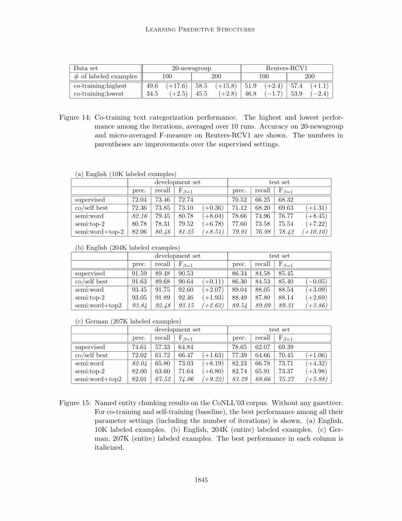
Learning Predictive Structures
Data set 20-newsgroup Reuters-RCV1# of labeled examples 100 200 100 200
co-training:highest 49.6 (+17.6) 58.5 (+15.8) 51.9 (+2.4) 57.4 (+1.1)co-training:lowest 34.5 (+2.5) 45.5 (+2.8) 46.8 (−1.7) 53.9 (−2.4)
Figure 14: Co-training text categorization performance. The highest and lowest perfor-mance among the iterations, averaged over 10 runs. Accuracy on 20-newsgroupand micro-averaged F-measure on Reuters-RCV1 are shown. The numbers inparentheses are improvements over the supervised settings.
(a) English (10K labeled examples)development set test set
prec. recall Fβ=1 prec. recall Fβ=1
supervised 72.04 73.46 72.74 70.52 66.25 68.32co/self best 72.36 73.85 73.10 (+0.36) 71.12 68.20 69.63 (+1.31)semi:word 82.16 79.45 80.78 (+8.04) 78.66 74.96 76.77 (+8.45)semi:top-2 80.78 78.31 79.52 (+6.78) 77.60 73.58 75.54 (+7.22)semi:word+top-2 82.06 80.46 81.25 (+8.51) 79.91 76.98 78.42 (+10.10)
(b) English (204K labeled examples)development set test set
prec. recall Fβ=1 prec. recall Fβ=1
supervised 91.59 89.48 90.53 86.34 84.58 85.45co/self best 91.63 89.68 90.64 (+0.11) 86.30 84.53 85.40 (−0.05)semi:word 93.45 91.75 92.60 (+2.07) 89.04 88.05 88.54 (+3.09)semi:top-2 93.05 91.89 92.46 (+1.93) 88.49 87.80 88.14 (+2.69)semi:word+top2 93.84 92.48 93.15 (+2.62) 89.54 89.09 89.31 (+3.86)
(c) German (207K labeled examples)development set test set
prec. recall Fβ=1 prec. recall Fβ=1
supervised 74.61 57.33 64.84 78.65 62.07 69.39co/self best 72.02 61.72 66.47 (+1.63) 77.39 64.66 70.45 (+1.06)semi:word 82.04 65.80 73.03 (+8.19) 82.23 66.78 73.71 (+4.32)semi:top-2 82.00 63.60 71.64 (+6.80) 82.74 65.91 73.37 (+3.98)semi:word+top2 82.01 67.52 74.06 (+9.22) 83.29 68.66 75.27 (+5.88)
Figure 15: Named entity chunking results on the CoNLL’03 corpus. Without any gazetteer.For co-training and self-training (baseline), the best performance among all theirparameter settings (including the number of iterations) is shown. (a) English,10K labeled examples. (b) English, 204K (entire) labeled examples. (c) Ger-man, 207K (entire) labeled examples. The best performance in each column isitalicized.
1845
Ando and Zhang
6. Discussions
This paper presents a general framework for learning predictive functional structures frommultiple tasks. The idea is based on the concept that if multiple problems share a commonpredictive structure, then the structure can be more reliably estimated by considering theseproblems together. The process of learning the shared functional structure is referred toas structural learning. In the learning theory framework, structural learning is to discovera common structure of the hypothesis spaces shared by the problems. The main theoret-ical justification of this approach is that the shared structural parameter can be reliablyestimated when m is large. Using the optimally estimated structural parameter, bettergeneralization performance (averaged over the problems) can be achieved.
Moreover, we showed that the framework of structural learning can be applied to semi-supervised learning. This is achieved by creating auxiliary problems from unlabeled datathat can reveal important underlying predictive structures of the data. Some examples ofauxiliary problems were provided, and experimental results demonstrated that the discov-ered structures are very useful. Rigorously speaking, the theory we developed in Appendix Adoes not directly apply to semi-supervised learning. This is because in our theory, the per-formance is measured by averaged generalization ability over multiple prediction problems.However, in the setting of semi-supervised learning, we are only interested in the perfor-mance of the original supervised task, and not any of the auxiliary problems. For semi-supervised learning, a more relevant consequence of our analysis is that the shared structurecan be stably estimated from multiple tasks. The usefulness of the shared structure is adifferent issue which is not directly answered by Appendix A. An intuitive justificationof auxiliary problems we created is given in Section 4.3, although a more complete theoryrequires further investigation.
In summary, our approach to semi-supervised learning makes a bet on the existence ofa shared predictive structure useful both for the supervised problem and for the auxiliaryproblems. The method proposed in Section 3 is robust since even if the discovered structuredoes not help on the supervised problem, the only potential negative effect is the introduc-tion of some non-predictive features. Using typical discriminative learning methods withappropriate regularization, a small number of bad features only have a minor impact on theperformance. However, if some of the features discovered from the auxiliary problems areuseful, then the performance improvement can be significant.
The method derived in Section 3 has the intuitive interpretation of discovering lowdimensional predictive structures on the classifier space. In our model, the most predictivedimensions correspond to the principal components of the multiple classifiers. Althoughour algorithm is based on the joint empirical risk minimization method which has a strongfoundation in learning theory (see Appendix A), in principle, we can consider a more generalapproach of mining structures in the classifier space. Based on this general principle, onecan design other structural learning algorithms that are not necessarily based on the jointempirical risk minimization method proposed in the paper. In fact, this general principle,which we may call structural mining, is the heart of our analysis. We shall thus concludethis paper by comparing some underlying concepts of structural mining to those of data-mining in Figure 16. In the table, a predictor can be regarded as a real-valued functiondefined on the data-space. The final row points out that we may also consider a data point
1846
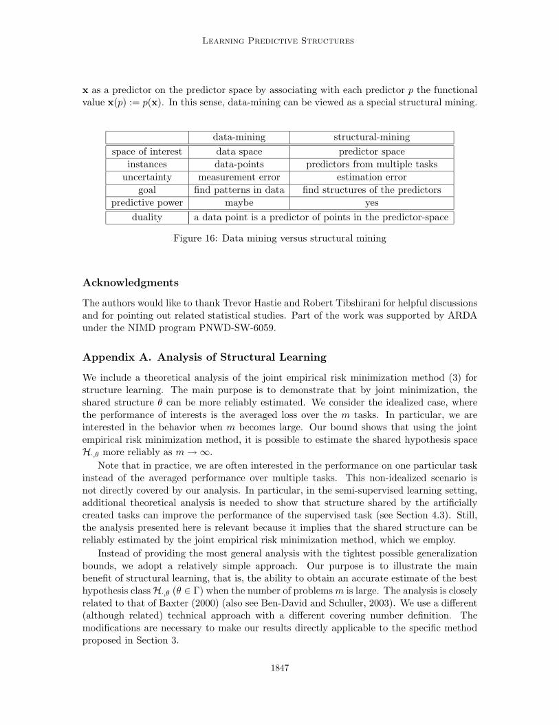
Learning Predictive Structures
x as a predictor on the predictor space by associating with each predictor p the functionalvalue x(p) := p(x). In this sense, data-mining can be viewed as a special structural mining.
data-mining structural-mining
space of interest data space predictor space
instances data-points predictors from multiple tasks
uncertainty measurement error estimation error
goal find patterns in data find structures of the predictors
predictive power maybe yes
duality a data point is a predictor of points in the predictor-space
Figure 16: Data mining versus structural mining
Acknowledgments
The authors would like to thank Trevor Hastie and Robert Tibshirani for helpful discussionsand for pointing out related statistical studies. Part of the work was supported by ARDAunder the NIMD program PNWD-SW-6059.
Appendix A. Analysis of Structural Learning
We include a theoretical analysis of the joint empirical risk minimization method (3) forstructure learning. The main purpose is to demonstrate that by joint minimization, theshared structure θ can be more reliably estimated. We consider the idealized case, wherethe performance of interests is the averaged loss over the m tasks. In particular, we areinterested in the behavior when m becomes large. Our bound shows that using the jointempirical risk minimization method, it is possible to estimate the shared hypothesis spaceH·,θ more reliably as m → ∞.
Note that in practice, we are often interested in the performance on one particular taskinstead of the averaged performance over multiple tasks. This non-idealized scenario isnot directly covered by our analysis. In particular, in the semi-supervised learning setting,additional theoretical analysis is needed to show that structure shared by the artificiallycreated tasks can improve the performance of the supervised task (see Section 4.3). Still,the analysis presented here is relevant because it implies that the shared structure can bereliably estimated by the joint empirical risk minimization method, which we employ.
Instead of providing the most general analysis with the tightest possible generalizationbounds, we adopt a relatively simple approach. Our purpose is to illustrate the mainbenefit of structural learning, that is, the ability to obtain an accurate estimate of the besthypothesis class H·,θ (θ ∈ Γ) when the number of problems m is large. The analysis is closelyrelated to that of Baxter (2000) (also see Ben-David and Schuller, 2003). We use a different(although related) technical approach with a different covering number definition. Themodifications are necessary to make our results directly applicable to the specific methodproposed in Section 3.
1847
Ando and Zhang
For clarity, in the following analysis, we simplify (3) as
[θ, {f`}] = arg minθ∈Γ,{f`∈Hθ}
m∑
`=1
n∑
i=1
L(f`(X`i), Y
`i ), (9)
where we only consider the case n1 = n2 = · · · = nm = n, and H1,θ = H2,θ = · · · =Hm,θ = Hθ. This simplification is not critical, but allows us to consider the behavior of (9)as m → ∞ under fixed n.
For simplicity, we use a covering-number approach in our analysis. The treatment isvery similar to the case of m = 1, which is the standard empirical risk minimization. Weneed to introduce some definitions in order to state the main theorem.
Definition 1 Consider a set V with a distance function d : V × V → {0} ∪ R+. Givenε > 0, the ε-covering number of V , denoted by N (ε, V, d(·, ·)), is the minimal number ofballs B(f) = {g : d(f, g) ≤ ε} of radius ε needed to cover V .
Definition 2 Let S(n) = {(X1, Y1), . . . , (Xn, Yn)} be a set of n points. We define the`2(S
(n)) distance between any two functions f(x, y) and g(x, y) on S(n) as
`2(S(n))(f, g) =
(
1
n
n∑
i=1
|f(Xi, Yi) − g(Xi, Yi)|2)1/2
.
Let F be a class of functions of (x, y). The empirical `2-covering number of F is thecovering number N (ε,F , `2(S
(n))) of F with respect to the `2(S(n)) distance. The uniform
`2 covering number is given by
N2(ε,F , n) = supS(n)
N (ε,F , `2(S(n))),
where the supremum is over all samples S(n) of size n.
Definition 3 Define distance d∞ between hypothesis spaces Hθ (θ ∈ Γ) as
d∞(θ1, θ2) = supf∈Hθ2
infg∈Hθ1
supx,y
|f(x, y) − g(x, y)|.
We define the d∞-covering number of Γ as N (ε, Γ, d∞).
The following theorem gives a (one-sided) uniform convergence result for the joint ERMmethod (9).
Theorem 4 For each ` = 1, . . . , m, let S` = {(X`i , Y
`i ), . . . , (X`
n, Y `n)} be a set of n points
for problem `, independently drawn from a distribution D`. Assume that L(f(x), y) is abounded Lipschitz function of f(x) ∈ Hθ. That is, there are θ-independent constants γ andM such that ∀θ1, θ2 ∈ Γ and ∀f1 ∈ Hθ1 , f2 ∈ Hθ2:
∀(x, y) : |L(f1(x), y) − L(f2(x), y)| ≤ γ|f1(x) − f2(x)|,∀(x1, y1), (x2, y2) : |L(f1(x1), y1) − L(f1(x2), y2)| ≤ M.
1848
Learning Predictive Structures
Then there is a universal constant C such that ∀η ∈ [0, 1], with probability 1 − η, we have∀θ, {f` ∈ Hθ}:
1
m
m∑
`=1
R`(f`) ≤1
m
m∑
`=1
R`(f`, S`) + γC infε0≥0
[
ε0 +
∫ ∞
ε0
√
lnN (ε)
ndε
]
+ M
√
ln 1η
nm,
where R` and R` are the true and empirical risks for problem `:
R`(f`) = E(X`,Y `)∼D`L(f`(X
`), Y `), R`(f`, S`) =1
n
n∑
i=1
L(f`(X`i), Y
`i ),
and
lnN (ε) = supθ
lnN2(ε,Hθ, n) +1
mlnN (ε, Γ, d∞).
We shall delay the proof to the end of this appendix, and discuss the implicationsof the theorem first. In summary, this result justifies the joint ERM method (9), whichminimizes the empirical risk on the right hand side of Theorem 4. The theorem impliesthat this method implicitly minimizes an upper bound of the true risk (averaged over the mproblems) on the left hand side, which leads to a theoretical guarantee of the performanceof this method.
The statistical complexity of the joint ERM method depends on the joint entropylnN (ε), which has two components: the first term supθ lnN2(ε,Hθ, n) is the learning com-plexity associated with individual estimation problems (with fixed θ). The second term1m lnN (ε, Γ, d∞) is the complexity of estimating the best structural parameter θ. The mostimportant consequence of our analysis is that the complexity of the structural space Γ,measured by the discounted entropy 1
m lnN (ε, Γ, d∞), approaches zero when m → ∞. Thisimplies that we are able to find a near optimal (as measured by the generalization bound)shared structural parameter θ when m is large.
This theorem can be used to analyze the method we propose in Section 3, where in (4)and (5), a bi-linear structural model of the following form is used:
HΘ =
{
wTΦ(x) + vT ΘΨ(x) : ‖w‖2 ≤ A
supx ‖Φ(x)‖2, ‖v‖2 ≤ B
supx ‖Ψ(x)‖2
}
,
Γ ={Θ ∈ Rh×p : ΘΘT = Ih×h},
where Φ(x) and Ψ(x) are pre-defined vector functions (feature maps) of x; v is an h-dimensional vector; Ψ(x) is a p-dimensional vector; and Θ is an orthonormal h × p dimen-sional matrix. We also use Ih×h to denote the h-dimensional identity matrix.
For this model, the matrix Θ, shared by the different prediction problems, is the struc-tural parameter. When we fix Θ, the hypothesis space HΘ is parameterized by weightvectors w and v, where w can be a high dimensional vector (regularized using A), andv is a low dimensional vector (of dimensionality h). The idea of this model is to find acommon low-dimensional predictive structure (shared by the m problems) parameterizedby the projection matrix Θ. If we can discover such a structure, then we only need to use
1849
Ando and Zhang
a very small A to regularize the w vector, which leads to improved generalization perfor-mance. In other words, there is a trade-off between the dimensionality h of the commonlow-dimensional predictive structure, and the regularization size A. The optimal trade-offis through the shared structural parameter Θ, which can be more reliably estimated usingstructural learning formulation (3) when m is large.
This intuitive argument can be more rigorously justified using Theorem 4 with appro-priate covering number estimates. Specifically, it can be shown that there are universalconstants C1, C2 and C3 such that
supθ
lnN2(ε,Hθ, n) ≤ C1A2
ε2+ C2h ln
(
1 +B
ε
)
, lnN (ε, Γ, d∞) ≤ C3hp ln
(
1 +B
ε
)
.
We shall not include a detailed proof of these estimates (which is not essential for the purposeof this paper) but only outline the basic ideas used in our derivation. The term C1A
2/ε2
follows from a simple estimate of the Rademacher complexity of the sub function classin HΘ corresponding to wTΦ(x) as A/
√n, and a straight-forward application of Sudak’s
minoration (e.g., see Ledoux and Talagrand, 1991, Chapter 12). The two ln(1+B/ε) termscan be obtained by explicit discretization of the corresponding finite dimensional parameterspaces — one for the h-dimensional sub function class in HΘ corresponding to vT ΘΨ(x)(with fixed Θ and variable v), and the other for a direct discretization of the hp-dimensionalvariable Θ. We simply note that a bounded set in a d-dimensional parameter space can becovered by O(ε−d) grid points with width no greater than ε in every direction.
By using the above covering number estimates, the complexity term in Theorem 4becomes
lnN (ε) ≤ C1A2
ε2+ C2h ln
(
1 +B
ε
)
+1
mC3hp ln
(
1 +B
ε
)
.
The third term is the complexity of estimating the structural parameter Θ, which vanishesas m → ∞. The first and second terms characterize the trade-off between the regulariza-tion size A for the w parameter, and the dimensionality h for the v parameter. With theestimated Θ, the model approximates the underlying true predictor better for a fixed reg-ularization size A (and thus a fixed complexity term lnN (ε) in Theorem 4), which impliesbetter generalization behavior.
Proof of Theorem 4 Given training data S = ∪`S`, we define a vector function class onS:
FS = {f = [f`] : f(X`i) = f`(X
`i), f` ∈ Hθ, θ ∈ Γ},
where we use the notation [f`] = [f`]`=1,...,m = [f1, . . . , fm]. Similarly, define
FLS = {[L(f(X`
i ), Y`i )]`=1,...,m : f ∈ FS}.
We introduce two lemmas.
Lemma 5 We have the following bounds:
ln N (2γε,FLS , `2(S)) ≤ ln N (2ε,FS , `2(S)) ≤
m∑
`=1
supθ
ln N (ε,Hθ, `2(S`)) + lnN (ε, Γ, d∞).
1850
Learning Predictive Structures
Proof The first inequality is a direct consequence of the Lipschitz condition in Theorem 4.We shall prove the second inequality. Consider an ε-cover of Γ in the d∞ metric. Forsimplicity, we denote the cover by θ1, . . . , θNΓ
, where NΓ = N (ε, Γ, d∞). For each θj , wecan find an ε-cover of Hθj
on S` as f`,j,1, . . . , f`,j,N`, where N` = N (ε,Hθ, `2(S`)).
Now given any f = [f`] ∈ FS , where f` ∈ Hθ for some θ ∈ Γ, we can find 1 ≤ J ≤ NΓ,and f ′ = [f ′
`] ∈ FS such that each f ′` ∈ HθJ
and `2(S)(f, f ′) ≤ ε. We can further approx-imate each f ′
` by a f`,J,K`where 1 ≤ K` ≤ N` such that `2(S`)(f
′`, f`,J,K`
) ≤ ε. It followsthat if we let f = [f`,J,K`
]`=1,...,m, then `2(S)(f ′, f) ≤ ε. Therefore we have `2(S)(f, f) ≤ 2ε.This means that FS has a 2ε-cover of the form f = [f`,J,K`
] (J = 1, . . . , NΓ, K` = 1, . . . , N`
for ` = 1, . . . , m). The size of this cover is NΓ∏
` N`.
Lemma 6 Let
Q(S) = sup[f`]∈FS
1
m
m∑
`=1
(R`(f`) − R`(f`, S`)),
then ∀η ∈ [0, 1], with probability 1 − η:
Q(S) ≤ ES Q(S) + M
√
ln 1η
mn.
Proof For a given 1 ≤ ¯≤ m and 1 ≤ i, we create a new dataset S = ∪`S` by changingthe i-th datum of the ¯-th problem in S = ∪`S` from (X
¯
i, Y
¯
i) to (X
¯
i, Y
¯
i) (and keep all the
other data points identical). Then it is easy to verify that
Q(S) − Q(S) ≤ supθ
supf∈Hθ
1
mn|L(f(X
¯
i ), Y¯
i ) − L(f(X¯
i ), Y¯
i )| ≤ M
mn.
The lemma is a direct consequence of McDiarmid’s concentration inequality (McDiarmid,1989).
We are now ready to prove the main theorem. Consider a sequence of binary randomvariables σ = {σ`
i} such that each σ`i = ±1 is independent with probability 1/2. The
Rademacher complexity of FLS under empirical sample S, is given by
R(FLS , S) = Eσ sup
f∈FS
(
1
mn
m∑
`=1
n∑
i=1
σ`iL(f(X`
i), Y`i )
)
.
It is well known that there exists a universal constant C (a variant of Corollary 2.2.8 invan der Vaart and Wellner, 1996):
R(FLS , S) ≤ C
2infε0
[
ε0 +1√mn
∫ ∞
ε0
√
lnN2(2ε,FLS , nm)dε
]
.
1851
Ando and Zhang
Applying Lemma 5, we obtain
R(FLS , S) ≤ C
2infε0
[
ε0 +
∫ ∞
ε0
√
lnN (ε/γ)
ndε
]
=γC
2infε0
[
ε0 +
∫ ∞
ε0
√
lnN (ε)
ndε
]
.
Using the standard symmetrization argument (for example, see Lemma 2.3.1 of (van derVaart and Wellner, 1996)), we have
ES Q(S) ≤ 2ES R(FLS , S) = γC inf
ε0
[
ε0 +
∫ ∞
ε0
√
lnN (ε)
ndε
]
.
The theorem is now a direct consequence of Lemma 6.
References
R. K. Ando and T. Zhang. A high-performance semi-supervised learning method for textchunking. In ACL 05, 2005.
J. Baxter. A model for inductive bias learning. Journal of Artificial Intelligent Research,pages 149–198, 2000.
M. Belkin and P. Niyogi. Semi-supervised learning on Riemannian manifolds. MachineLearning, Special Issue on Clustering:209–239, 2004.
S. Ben-David and R. Schuller. Exploiting task relatedness for multiple task learning. InCOLT 03, 2003.
A. Blum and T. Mitchell. Combining labeled and unlabeled data with co-training. Inproceedings of the eleventh annual conference on Computational learning theory, pages92–100, 1998.
L. Breiman and J. Friedman. Predicting multivariate responses in multiple linear regression.J. Roy. Statist. Soc. B., 59:3–37, 1997. with discussion.
R. Caruana. Multi-task learning. Machine Learning, pages 41–75, 1997.
H. L. Chieu and H. T. Ng. Named entity recognition with a maximum entropy approach.In Proceedings CoNLL-2003, pages 160–163, 2003.
T. Evegniou and M. Pontil. Regularized multi–task learning. In Proc. Conf. on KnowledgeDiscovery and Data Mining, 2004.
R. Florian, A. Ittycheriah, H. Jing, and T. Zhang. Named entity recogintion throughclassifier combination. In Proceedings CoNLL-2003, pages 168–171, 2003.
T. Hastie, R. Tibshirani, and J. Friedman. The Elements of Statistical Learning. Springer,2001.
T. Joachims. Transductive inference for text classification using support vector machines.In Proceedings of the Sixteenth International Conference on Machine Learning, pages200–209, 1999.
1852
Learning Predictive Structures
D. Klein, J. Smarr, H. Nguyen, and C. D. Manning. Named entity recognition withcharacter-level models. In Proceedings CoNLL-2003, pages 188–191, 2003.
M. Ledoux and M. Talagrand. Probability in Banach spaces. Springer-Verlag, Berlin, 1991.ISBN 3-540-52013-9. Isoperimetry and processes.
C. McDiarmid. On the method of bounded differences. In Surveys in Combinatorics, pages148–188. Cambridge University Press, 1989.
C. A. Micchelli and M. Ponti. Kernels for multi–task learning. In NIPS 2004, 2005. toappear.
K. Nigam, A. K. McCallum, S. Thrun, and T. Mitchell. Text classification from labeledand unlabeled documents using EM. Machine Learning, Special issue on informationretrieval:103–134, 2000.
D. Pierce and C. Cardie. Limitations of co-training for natural language learning fromlarge datasets. In Proceedings of the 2001 Conference on Empirical Methods in NaturalLanguage Processing (EMNLP-2001), 2001.
M. Szummer and T. Jaakkola. Partially labeled classification with Markov random walks.In NIPS 2001, 2002.
A. W. van der Vaart and J. A. Wellner. Weak convergence and empirical processes. SpringerSeries in Statistics. Springer-Verlag, New York, 1996. ISBN 0-387-94640-3.
V. N. Vapnik. Statistical learning theory. John Wiley & Sons, New York, 1998.
D. Yarowsky. unsupervised word sense disambiguation rivaling supervised methods. Inproceedings of ACL 95, pages 189–196, 1995.
T. Zhang. Solving large scale linear prediction problems using stochastic gradient descentalgorithms. In ICML 04, pages 919–926, 2004.
T. Zhang and D. E. Johnson. A robust risk minimization based named entity recognitionsystem. In Proceedings CoNLL-2003, pages 204–207, 2003.
T. Zhang and F. J. Oles. A probability analysis on the value of unlabeled data for classifi-cation problems. In ICML 00, pages 1191–1198, 2000.
D. Zhou, O. Bousquet, T. N. Lal, J. Weston, and B. Schlkopf. Learning with local andglobal consistency. In NIPS 2003, pages 321–328, 2004.
X. Zhu, Z. Ghahramani, and J. Lafferty. Semi-supervised learning using gaussian fields andharmonic functions. In ICML 2003, 2003.
1853