Learning Model Predictive Control for Iterative Tasks. A Data-DrivenControl Framework.

Ugo Rosolia and Francesco Borrelli

Abstract— A Learning Model Predictive Controller (LMPC)for iterative tasks is presented. The controller is reference-free and is able to improve its performance by learning fromprevious iterations. A safe set and a terminal cost functionare used in order to guarantee recursive feasibility and non-decreasing performance at each iteration. The paper presentsthe control design approach, and shows how to recursivelyconstruct terminal set and terminal cost from state and inputtrajectories of previous iterations. Simulation results show theeffectiveness of the proposed control logic.

I. INTRODUCTION

Control systems autonomously performing a repetitive taskhave been extensively studied in the literature [1], [2], [3],[4], [5], [6]. One task execution is often referred to as“iteration” or “trial”. Iterative Learning Control (ILC) is acontrol strategy that allows learning from previous iterationsto improve its closed-loop tracking performance. In ILC,at each iteration, the system starts from the same initialcondition and the controller objective is to track a givenreference, rejecting periodic disturbances [1], [3]. The mainadvantage of ILC is that information from previous iterationsare incorporated in the problem formulation at the nextiteration and are used to improve the system performance.The possibility of combining MPC with ILC has beenexplored in [7], where the authors proposed a Model-basedPredictive Control for Batch processes (MPCB). The BMPCis based on a time-varying MIMO system that has a dynamicmemory of past batches tracking error. The effectiveness ofthis approach has been shown through experimental resultson a nonlinear system [7], and in [8] the authors provedthat the tracking error of the BMPC converges to zero as thenumber of iterations increases. In [9] a model-based iterativelearning control has been proposed. The authors incorporatedthe tracking error of the previous iterations in the control lawand used an observer to deal with stochastic disturbancesand noises. Also in this case, the authors showed that thetracking error asymptotically converges to zero. Anotherstudy on Model Predictive Control (MPC) for repetitivetasks has appeared in [2]. The authors successfully achievezero tracking error using a MPC which uses measurementsfrom previous iterations to modify the cost function. In [10]the authors use the trajectories of previous iterations tolinearize the model used in the MPC algorithm. The authorsproved zero steady-state tracking error in presence of modelmismatch. In the aforementioned papers the control goal is to

Ugo Rosolia and Francesco Borrelli are with the Department of Mechani-cal Engineering, University of California at Berkeley , Berkeley, CA 94701,USA {ugo.rosolia, fborrelli} @ berkeley.edu

minimize a tracking error under the presence of disturbances.The reference signal is known in advance and does notchange at each iteration.

In this paper we are interested in repetitive tasks where thereference trajectory it is not known. In general, a referencetrajectory that maximize the performance over an infinitehorizon may be challenging to compute for a system withcomplex nonlinear dynamics or with parameter uncertainty.These systems include race and rally cars where the envi-ronment and the dynamics are complex and not perfectlyknown [11], [12], or bipedal locomotion with exoskeletonswhere the human input is unknown apriori and can changeat each iteration [13], [14].

Our objective is to design a reference-free iterative controlstrategy able to learn from previous iterations. At eachiteration the cost associated with the closed-loop trajectoryshall not increase and state and input constraints shall besatisfied. Nonlinear Model Predictive control is an appealingtechnique to tackle this problem for its ability to handlestate and inputs constraints while minimizing a finite-timepredicted cost [15]. However, the receding horizon naturecan lead to infeasibility and it does not guaranty improvedperformance at each iteration [16].

The contribution of this paper is threefold. First we presenta novel reference-free learning MPC design for an iterativecontrol task. At each iteration, the initial condition, theconstraints and the objective function do not change. The j-th iteration cost is defined as the objective function evaluatedfor the j-th closed loop system trajectory. Second, we showhow to design a terminal safe set and a terminal cost functionin order to guarantee that (i): the j-th iteration cost does notincrease compared to the j-1-th iteration cost (non-increasingcost at each iteration), (ii): state and input constraints aresatisfied at iterations j if they were satisfied at iterationj-1 (recursive feasibility), (iii): the closed-loop equilibriumis asymptotically stable. Third, we assume that the systemconverges to a steady state trajectory as the number ofiteration j goes to infinity and we prove the local optimalityof such trajectory.

This paper is organized as follows: in Section II weformally define an iterative task and its j-th iteration cost.The control strategy is illustrated in Section III. Firstly, weshow the recursive feasibility and stability of the controllogic and, afterwards, we prove the convergence properties.Finally, in Section IV and V, we test the proposed controllogic on an infinite horizon linear quadratic regulator withconstraints and on a minimum time Dubins car problem.Section VI and VII provide final remarks.

II. PROBLEM DEFINITION

Consider the discrete time system

xt+1 = f(xt, ut), (1)

where the dynamic update f(·, ·) is continuous, x ∈ Rn andu ∈ Rm are the system state and input, respectively, subjectto the constraints

xt ∈ X , ut ∈ U , ∀t ∈ Z0+. (2)

At the j-th iteration the vectors

uj = [uj0, uj1, ..., u

jt , ...], (3a)

xj = [xj0, xj1, ..., x

jt , ...], (3b)

collect the inputs applied to system (1) and the correspondingstate evolution. In (3), xjt and ujt denote the system state andthe control input at time t of the j-th iteration. We assumethat at each j-th iteration the closed loop trajectories startfrom the same initial state,

xj0 = xS , ∀j ≥ 0. (4)

The goal is to design a controller which solves thefollowing infinite horizon optimal control problem at eachiteration:

J∗0→∞(xS) = minu0,u1,...

∞∑k=0

h(xk, uk) (5a)

s.t. xk+1 = f(xk, uk), ∀k ≥ 0 (5b)x0 = xS , (5c)xk ∈ X , uk ∈ U , ∀k ≥ 0 (5d)

where equations (5b) and (5c) represent the system dynamicsand the initial condition, and (5d) are the state and input con-straints. The stage cost, h(·, ·), in equation (5a) is continuousand it satisfies

h(xF , 0) = 0 and h(xjt , ujt ) � 0 ∀ xjt ∈ Rn \ {xF },

ujt ∈ Rm \ {0},(6)

where the final state xF is assumed to be a feasible equilib-rium for the unforced system (1)

f(xF , 0) = xF . (7)

Throughout the paper we assume that a local optimal solutionto Problem (5) exists and it is denoted as:

x∗ = [x∗0, x∗1, ..., x

∗t , ...],

u∗ = [u∗0, u∗1, ..., u

∗t , ...].

(8)

Remark 1: The stage cost, h(·, ·), in (6) is strictly positiveand zero at xF . Thus, an optimal solution to (5) convergesto the final point xF , i.e. limt→∞ x∗t = xF .

Remark 2: In practical applications each iteration has afinite-time duration. It is common in the literature to adoptan infinite time formulation at each iteration for the sakeof simplicity. We follow such an approach in this paper.

Our choice does not affect the practicality of the proposedmethod.

Next we introduce the definition of the sampled safe setand of the iteration cost. Both which will be used later toguarantee stability and feasibility of the learning MPC.

A. Sampled Safe SetDefinition 1 (one-step controllable set to the set S): For

the system (1) we denote the one-step controllable set tothe set S as

K1(S) = Pre(S) ∩ X . (9)

where

Pre(S) , {x ∈ Rn : ∃u ∈ U s.t. f(x, u) ∈ S}. (10)

K1(S) is the set of states which can be driven into thetarget set S in one time step while satisfying input and stateconstraints. N -step controllable sets are defined by iteratingK1(S) computations.

Definition 2 (N -Step Controllable Set KN (S)): For agiven target set S ⊆ X , the N -step controllable set KN (S)of the system (1) subject to the constraints (2) is definedrecursively as:

Kj(S) , Pre(Kj−1(S))∩X , K0(S) = S, j ∈ {1, . . . , N}(11)

From Definition 2, all states x0 of the system (1) belongingto the N -Step Controllable Set KN (S) can be driven, bya suitable control sequence, to the target set S in N steps,while satisfying input and state constraints.

Definition 3 (Maximal Controllable Set K∞(O)): For agiven target set O ⊆ X , the maximal controllable set K∞(O)for system (1) subject to the constraints in (2) is the union ofall N -step controllable sets KN (O) contained in X (N ∈ N).We will use controllable sets KN (O) where the target Ois a control invariant set [17]. They are special sets, sincein addition to guaranteeing that from KN (O) we reach Oin N steps, one can ensure that once it has reached O, thesystem can stay there at all future time instants. These setsare called control invariant set.Note that xF in (7) is a control invariant since it is anequilibrium point.

Definition 4 (N -step (Maximal) Stabilizable Set): For agiven control invariant set O ⊆ X , the N -step (maximal)stabilizable set of the system (1) subject to the constraints (2)is the N -step (maximal) controllable set KN (O) (K∞(O)).

Since the computation of Pre-set is numerically challeng-ing for nonlinear systems, there is extensive literature onhow to obtain an approximation (often conservative) of theMaximal Stabilizable Set [18].

In this paper we exploit the iterative nature of the controldesign and define the sampled Safe Set SSj at iteration j as

SSj =

{ ⋃i∈Mj

∞⋃t=0

xit

}. (12)

SSj is the collection of all state trajectories at iteration ifor i ∈ M j . M j in equation (12) is the set of indexes kassociated with successful iterations k for k ≤ j, defined as:

M j ={k ∈ [0, j] : lim

t→∞xkt = xF

}. (13)

From (13) we have that M i ⊆ M j ,∀i ≤ j, which impliesthat

SSi ⊆ SSj ,∀i ≤ j. (14)

Figure 1 shows an example of the sampled safe set phaseplot, for a two state system.

Remark 3: Note that SSj can be interpreted as a sampledsubset of the Maximal Stabilizable Set K∞(xF ) as for everypoint in the set, there exists a feasible control action whichsatisfies the state constraints and steers the state towardsxF .

xF

Safe Set

Fig. 1. The circled dots represent the sampled safe set (SS) in a twodimensional phase plane, collecting three successful trajectories.

B. Iteration Cost

At time t of the j-th iteration the cost-to-go associatedwith the closed loop trajectory (3b) and input sequence (3a)is defined as

Jjt→∞(xjt ) =

∞∑k=t

h(xjk, ujk), (15)

where h(·, ·) is the stage cost of the problem (5). We definethe j-th iteration cost as the cost (15) of the j-th trajectoryat time t = 0,

Jj0→∞(xj0) =

∞∑k=0

h(xjk, ujk). (16)

Jj0→∞(xj0) quantifies the controller performance at eachj-th iteration.

Remark 4: In equations (16)-(15), xjk and ujk are therealized state and input at the j-th iteration, as defined in (3).

Remark 5: At each j-th iteration the system is initializedat the same starting point xj0 = xS ; thus we haveJj0→∞(xj0) = Jj0→∞(xS).

Finally, we define the function Qj(·), defined over thesample safe set SSj as:

Qj(x) =

min(i,t)∈F j(x)

J it→∞(x), if x ∈ SSj

+∞, if x /∈ SSj, (17)

where F j(·) in (17) is defined as

F j(x) ={

(i, t) : i ∈ [0, j], t ≥ 0 with x = xit;

for xit ∈ SSj}.

(18)

Remark 6: The function Qj(·) in (17) assigns to everypoint in the sampled safe set, SSj , the minimum cost-to-goalong the trajectories in SSj i.e.,

∀x ∈ SSj , Qj(x) = J i∗

t∗→∞(x) =

∞∑k=t∗

h(xi∗

k , ui∗

k ), (19)

where the indices pair (i∗, t∗) is the minimizer in (17):

(i∗, t∗) = argmin(i,t)∈F j(x)

J it→∞(x), for x ∈ SSj . (20)In the next section we exploit the fact that at each

iteration we solve the same problem to design a controllerthat guarantees a non-increasing iteration cost (i.e.Jj0→∞(·) ≤ Jj−1

0→∞(·)) and which converges to a localoptimal solution of (5) (i.e. limj→∞ xj = x∗ andlimj→∞ uj = u∗).

III. LMPC CONTROL DESIGNIn this section we present the design of the proposed

Learning Model Predictive Control (LMPC). We first assumethat there exists an iteration where the LMPC is feasible atall time instants. Then we prove that the proposed LMPC isguaranteed to be recursively feasible, i.e. feasible at all timeinstants of every successive iteration. Moreover, the trajec-tories from previous iterations are used to guarantee non-increasing iterations cost between two successive iterations.Finally, we show that the proposed approach converges to alocal optimum of the infinite horizon control problem (5).

A. LMPC FormulationThe LMPC tries to compute a solution to the infinite time

optimal control problem (5) by solving at time t of iterationj the finite time constrained optimal control problem

J LMPC,jt→t+N (xjt ) = min

ut|t,...,ut+N−1|t

[ t+N−1∑k=t

h(xk|t, uk|t)+

+Qj−1(xt+N |t)

](21a)

s.t.xk+1|t = f(xk|t, uk|t), ∀k ∈ [t, · · · , t+N − 1] (21b)

xt|t = xjt , (21c)xk|t ∈ X , uk ∈ U , ∀k ∈ [t, · · · , t+N − 1] (21d)

xt+N |t ∈ SSj−1, (21e)

where (21b) and (21c) represent the system dynamics andinitial condition, respectively. The state and input constraintsare given by (21d). Finally (21e) forces the terminal state intothe set SSj−1 defined in equation (12).Let

u∗,jt:t+N |t = [u∗,jt|t , · · · , u∗,jt+N−1|t]

x∗,jt:t+N |t = [x∗,jt|t , · · · , x∗,jt+N |t]

(22)

be the optimal solution of (21) at time t of the j-th iterationand J LMPC,j

t→t+N (xjt ) the corresponding optimal cost. Then, attime t of the iteration j, the first element of u∗,jt:t+N |t isapplied to the system (1)

ujt = u∗,jt|t . (23)

The finite time optimal control problem (21) is repeatedat time t + 1, based on the new state xt+1|t+1 = xjt+1

(21c), yielding a moving or receding horizon control strategy.

Assumption 1: At iteration j = 1 we assume thatSSj−1 = SS0 is a non-empty set and that the trajectoryx0 ∈ SS0 is feasible and convergent to xF .

Assumption 1 is not restrictive in practice for a numberof applications. For instance, with race cars one can alwaysrun a path following controller at very low speed to obtaina feasible state and input sequence.

In the next section we prove that, under Assumption 1,the LMPC (21) and (23) in closed loop with system (1)guarantees recursively feasibility and stability, and non-increase of the iteration cost at each iteration.

Remark 7: From (12), SSj at the j-th iteration is the setof all successful trajectories performed in the first j trials.We assume that these trajectories can be recorded and storedat each iteration. Checking if a state is in SSj is a simplesearch. However, the optimization problem (21) becomeschallenging to solve even in the linear case due to the integernature of the constraints (21e). In Section VI.A we commenton practical approaches to improve the computational timeto solve (21).

B. Recursive feasibility and stability

As mentioned in Section II, for every point in the set SSjthere exists a control sequence that can drive the systemto the terminal point xF . The properties of SSj and Qj(·)are used in the next proof to show recursive feasibility andasymptotic stability of the equilibrium point xF .

Theorem 1: Consider system (1) controlled by the LMPCcontroller (21) and (23). Let SSj be the sampled safe set atiteration j as defined in (12). Let assumption 1 hold, then

the LMPC (21) and (23) is feasible ∀ t ∈ Z0+ and iterationj ≥ 1. Moreover, the equilibrium point xF is asymptoticallystable for the closed loop system (1) and (23) at everyiteration j ≥ 1.The proof follows from standard MPC arguments.

Proof: By assumption SS0 is non empty. From (14) wehave that SS0 ⊆ SSj−1 ∀j ≥ 1, and consequently SSj−1 isa non empty set. In particular, there exists a trajectory x0 ∈SS0 ⊆ SSj−1. From (4) we know that xj0 = xS ∀j ≥ 0. Attime t = 0 of the j-th iteration the N steps trajectory

[x00, x

01, ..., x

0N ] ∈ SSj−1, (24)

and the related input sequence,

[u00, u

01, ..., u

0N−1], (25)

satisfy input and state constrains (21b)-(21c)-(21d). There-fore (24)-(25) is a feasible solution to the LMPC (21) and(23) at t = 0 of the j-th iteration.Assume that at time t of the j-th iteration the LMPC (21)and (23) is feasible and let x∗,jt:t+N |t and u∗,jt:t+N |t be theoptimal trajectory and input sequence, as defined in (22).From (21c) and (23) the realized state and input at time t ofthe j-th iteration are given by

xjt = x∗,jt|t ,

ujt = u∗,jt|t .(26)

Moreover, the terminal constraint (21e) enforces x∗,jt+N |t ∈SSj−1 and, from (19),

Qj−1(x∗,jt+N |t) = J i∗

t∗→∞(x∗,jt+N |t) =

∞∑k=t∗

h(xi∗

k , ui∗

k ). (27)

Note that xi∗

t∗+1 = f(xi∗

t∗ , ui∗

t∗) and, by the definition of Qj(·)and F j(x) in (17)-(18), xi

∗

t∗ = x∗,jt+N |t. Since the state updatein (1) and (21b) are assumed identical we have that

xjt+1 = x∗,jt+1|t. (28)

At time t+ 1 of the j-th iteration the input sequence

[u∗,jt+1|t, u∗,jt+2|t, ..., u

∗,jt+N−1|t, u

i∗

t∗ ], (29)

and the related feasible state trajectory

[x∗,jt+1|t, x∗,jt+2|t, ..., x

∗,jt+N−1|t, x

i∗

t∗ , xi∗

t∗+1] (30)

satisfy input and state constrains (21b)-(21c)-(21d).Therefore, (29)-(30) is a feasible solution for the LMPC(21) and (23) at time t+ 1.We showed that at the j-th iteration, ∀j ≥ 1 , (i): the LMPCis feasible at time t = 0 and (ii): if the LMPC is feasible at

time t, then the LMPC is feasible at time t + 1. Thus, weconclude by induction that the LMPC in (21) and (23) isfeasible ∀j ≥ 1 and t ∈ Z0+.

Next we use the fact the Problem (21) is time-invariant ateach iteration j and we replace J LMPC,j

t→t+N (·) with J LMPC,j0→N (·).

In order to show the asymptotic stability of xF we have toshow that the optimal cost, J LMPC,j

0→N (·), is a Lyapunov functionfor the equilibrium point xF (7) of the closed loop system(1) and (23) [17]. Continuity of J LMPC,j

0→N (·) can be shown as in[16]. Moreover from (5a), J LMPC,j

0→N (x) � 0 ∀ x ∈ Rn \ {xF }and J LMPC,j

0→N (xF ) = 0. Thus, we need to show that J LMPC,j0→N (·)

is decreasing along the closed loop trajectory.From (28) we have x∗,jt+1|t = xjt+1, which implies that

J LMPC,j0→N (x∗t+1|t) = J LMPC,j

0→N (xjt+1). (31)

Given the optimal input sequence and the related optimaltrajectory in (22), the optimal cost is given by

J LMPC,j0→N (xjt ) = min

ut|t,...,ut+N−1|t

[N−1∑k=0

h(xk|t, uk|t)+

+Qj−1(xN |t)

]=

= h(x∗,jt|t , u∗,jt|t ) +

N−1∑k=1

h(x∗,jt+k|t, u∗,jt+k|t) +Qj−1(x∗,jt+N |t) =

= h(x∗,jt|t , u∗,jt|t ) +

N−1∑k=1

h(x∗,jt+k|t, u∗,jt+k|t) + J i

∗

t∗→∞(x∗,jt+N |t) =

= h(x∗,jt|t , u∗,jt|t ) +

N−1∑k=1

h(x∗,jt+k|t, u∗,jt+k|t) +

∞∑k=t∗

h(xi∗

k , ui∗

k ) =

= h(x∗,jt|t , u∗,jt|t ) +

N−1∑k=1

h(x∗,jt+k|t, u∗,jt+k|t) + h(xi

∗

t∗ , ui∗

t∗) +

+Qj−1(xi∗

t∗+1) ≥≥h(x∗,jt|t , u

∗,jt|t ) + J LMPC,j

0→N (x∗,jt+1|t),(32)

where i∗ is defined in (20).Finally, from equations (23), (26) and (31)-(32) we con-

clude that the optimal cost is a decreasing Lyapunov functionalong the closed loop trajectory,

J LMPC,j0→N (xjt+1)− J LMPC,j

0→N (xjt ) ≤ −h(xjt , ujt ) < 0,

∀ xjt ∈ Rn \ {xF }, ∀ ujt ∈ Rm \ {0}

(33)Equation (33), the positive definitiveness of h(·) and thecontinuity of J LMPC,j

0→N (·) imply that xF is asymptotically stable.�

C. Convergence properties

In this Section we assume that the LMPC (21) and (23)converges to a steady state trajectory. We show two results.First, the j-th iteration cost Jj0→∞(·) does not worsen asj increases. Second, the steady state trajectory is a localoptimal solution of the infinite horizon control problem(5). In this Section we use the fact the Problem (21) istime-invariant at each iteration j and we replace J LMPC,j

t→t+N (·)with J LMPC,j

0→N (·).

Theorem 2: Consider system (1) in closed loop with theLMPC controller (21) and (23). Let SSj be the sampled safeset at the j-th iteration as defined in (12). Let assumption1 hold, then the iteration cost Jj0→∞(·) does not increasewith the iteration index j.

Proof: First, we find a lower bound on the j-th iterationcost Jj0→∞(·), ∀ j > 0. Consider the realized state andinput sequence (3) at the j-th iteration, which collects thefirst element of the optimal state and input sequence to theLMPC (21) and (23) at time t, ∀t ∈ Z0+, as shown in (26).By the definition of the iteration cost in (15), we have

Jj−10→∞(xS) =

∞∑t=0

h(xj−1t , uj−1

t ) =

=

N−1∑t=0

h(xj−1t , uj−1

t ) +

∞∑t=N

h(xj−1t , uj−1

t ) ≥

≥N−1∑t=0

h(xj−1t , uj−1

t ) +Qj−1(xj−1N ) ≥

≥ minu0,...,uN−1

[N−1∑k=0

h(xk, uk) +Qj−1(xN )

]=

= J LMPC,j0→N (xj0).

(34)Then we notice that, at the j-th iteration, the optimal cost ofthe LMPC (21) and (23) at t = 0, J LMPC,j

0→N (xj0), can be upperbounded along the realized trajectory (3) using (33)

J LMPC,j0→N (xj0) ≥ h(xj0, u

j0) + J LMPC,j

0→N (xj1) ≥

≥ h(xj0, uj0) + h(xj1, u

j1) + J LMPC,j

0→N (xj2) ≥

≥ limT→∞

[T−1∑k=0

h(xjk, ujk) + J LMPC,j

0→N (xjT )

].

(35)

Note that J LMPC,j0→N (·) evaluated along the j-th closed loop

trajectory (3b) is a decreasing function convergent to zero.Furthermore, the sum of the stage costs, h(·, ·), in (35) isupper-bounded by the j-th iteration cost at time t = 0

J LMPC,j0→N (xj0), and therefore the limit in (35) is well defined.

Moreover, from Theorem 1 xF is asymptotically stable forthe closed loop system (1) and (23) (i.e. limt→∞ xjt = xF ),thus

J LMPC,j0→N (xj0) ≥ lim

T→∞

[T−1∑k=0

h(xjk, ujk) + J LMPC,j

0→N (xjT )

]=

=

∞∑k=0

h(xjk, ujk) = Jj0→∞(xS).

(36)

From equations (34)-(36) we conclude that

Jj−10→∞(xS) ≥ J LMPC,j

0→N (xj0) ≥ Jj0→∞(xS), (37)

thus the iteration cost is non-increasing. �

Theorem 3: Consider system (1) in closed loop with theLMPC controller (21) and (23). Let SSj be the sampled safeset at the j-th iteration as defined in (12). Let assumption1 hold and assume that the closed loop system (1) and(23) converges to a steady state trajectory x∞, for iterationj → ∞. Then, the steady state input u∞ = limj→∞ uj

and the related steady state trajectory x∞ = limj→∞ xj

is a local optimal solution for the infinite horizon optimalcontrol problem (5), i.e., x∞ = x∗ and u∞ = u∗.

Proof: By assumption, the closed loop system (1) and(23) converges to a steady state trajectory, x∞. By definitionboth the sampled safe set SSj and the terminal cost functionQj(·) converge to steady state quantities, denoted as SS∞and Q∞(·), respectively. In particular, from definition (12),we have that x∞ ∈ SS∞. From (33) we have that

J LMPC,∞0→N (x∞t ) ≥ h(x∞t , u

∞t ) + J LMPC,∞

0→N (x∞t+1) ≥

≥h(x∞t , u∞t ) + h(x∞t+1, u

∞t+1) + J LMPC,∞

0→N (x∞t+2) ≥

≥ limT→∞

[T−1∑k=0

h(x∞t+k, u∞t+k) + J LMPC,∞

0→N (x∞t+T )

].

(38)Moreover, from Theorem 1 we have that xF is asymptotically

stable for the closed loop system (1) and (23), thus

J LMPC,∞0→N (x∞t ) ≥ lim

T→∞

[T∑k=0

h(x∞t+k, u∞t+k) + J LMPC,∞

0→N (x∞t+T )

]=

=

∞∑k=0

h(x∞t+k, u∞t+k) =

=

N−1∑k=0

h(x∞t+k, u∞t+k) +

∞∑k=N

h(x∞t+k, u∞t+k).

(39)Note that in equation (39) x∞t+k ∈ SS∞, thus

J LMPC,∞0→N (x∞t ) ≥

N−1∑k=0

h(x∞t+k, u∞t+k) +

∞∑k=N

h(x∞t+k, u∞t+k) ≥

≥N−1∑k=0

h(x∞t+k, u∞t+k) +Q∞(x∞t+N ).

(40)In (40) the cost associated with the feasible trajectory

x∞t:t+N = [x∞t , x∞t+1, ..., x

∞t+N ] (41)

is a lower bound on the optimal cost J LMPC,∞0→N (x∞t ). Therefore,

the trajectory x∞t:t+N and the related input sequence

u∞t:t+N = [u∞t , u∞t+1, ..., u

∞t+N−1] (42)

is an optimal solution to the LMPC (21) and (23) at time tof the j-th iteration for j →∞.Next, we prove that x∞0:N+1 and u∞0:N+1 is a locally optimalsolution to the LMPC (21) and (23) where N is replacedwith N + 1. Consider the Hamiltonian

H(x, u, λ) = h(x, u) + f(x, u)Tλ, (43)

where h(x, u) and f(x, u) are the stage cost and the systemdynamics defined in equations (21) and (1), respectively. Theminimum principle [19] states that, if the state trajectory isoptimal, it exists a sequence of costate λ∞k such that:

x∞k+1 = Hλ(x∞k , u∞k , λ

∞k+1) (44a)

λ∞k = Hx(x∞k , u∞k , λ

∞k+1) (44b)

u∞k = argminuk

H(x∞k , uk, λ∞k+1). (44c)

Therefore, for the optimal solution to the LMPC (21) and(23) at time t = 0 of the j-th iteration for j → ∞, definedin (41)-(42),

x∞0:N = [x∞0 , x∞1 , ..., x

∞N ]

u∞0:N = [u∞0 , u∞1 , ..., u

∞N−1],

(45)

it exists a sequence of costate

[λ∞1 , λ∞2 , ..., λ

∞N ], (46)

that satisfies the minimum principle (44). Moreover, for theoptimal solution of the LMPC (21) and (23) at time t = 1of the j-th iteration for j →∞,

x∞1:1+N = [x∞1 , x∞2 , ..., x

∞N+1]

u∞1:1+N = [u∞1 , u∞2 , ..., u

∞N ],

(47)

there exists a vector λ∞ such that

[λ∞2 , λ∞3 , ..., λ

∞N+1] (48)

satisfies the minimum principle (44). Therefore, from equa-tions (43) and (44c) we have that

u∞k = h(x∞k , u∞k ) + f(x∞k , u

∞k )Tλ∞k+1 ∀k ∈ [0, N − 1]

u∞k = h(x∞k , u∞k ) + f(x∞k , u

∞k )T λ∞k+1 ∀k ∈ [1, N ],

(49)from this

λ∞k+1 = λ∞k+1, ∀k ∈ [1, N − 1]. (50)

Finally, we conclude that the N + 1 steps trajectory

x∞0:N+1 = [x∞0 , x∞1 , ..., x

∞N+1]

u∞0:N+1 = [u∞0 , u∞1 , ..., u

∞N ],

(51)

and the costate sequence

λ∞ = [λ∞1 , λ∞2 = λ∞2 , ..., λ

∞N = λ∞N , λ

∞N+1] (52)

satisfy the minimum principle. Therefore at time t = 0 ofthe j-th iteration for j → ∞, the trajectory and its relatedinput sequence,

x∞0:N+1 = [x∞0 , x∞1 , ..., x

∞N+1]

u∞0:N+1 = [u∞0 , u∞1 , ..., u

∞N ],

(53)

is a local optimal solution for the LMPC (21) and (23) withhorizon N+1 steps. Next, we show that the above procedurecan be iterated to prove local optimality of the N + 2 stepstrajectory x∞[0:N+2] and the related input sequence u∞[0:N+2]

for the LMPC (21) and (23) with N = N + 2. Let

[λ∞3 , λ∞4 , ..., λ

∞N+2] (54)

be the costate associated with the solution of the LMPC attime t = 2 of the j-th iteration for j →∞

x∞2:2+N = [x∞2 , x∞3 , ..., x

∞N+2]

u∞2:2+N = [u∞2 , u∞3 , ..., u

∞N+1].

(55)

We have, from equations (43) and (44c), and optimality ofthe trajectory in (53), that

u∞k = h(x∞k , u∞k ) + f(x∞k , u

∞k )T λ∞k+1 ∀k ∈ [0, N ]

u∞k = h(x∞k , u∞k ) + f(x∞k , u

∞k )T λ∞k+1 ∀k ∈ [2, N + 1],

(56)

from thisλ∞k+1 = λ∞k+1, ∀k ∈ [2, N ]. (57)

Therefore the N + 2 steps trajectory and the related costate

x∞0:N+2 = [x∞0 , x∞1 , ..., x

∞N+2]

u∞0:N+2 = [u∞0 , u∞1 , ..., u

∞N+1],

[λ∞1 , λ∞2 , λ

∞3 = λ∞3 , ..., λ

∞N+1 = λ∞N+1, λ

∞N+2]

(58)

satisfy the minimum principle and it is locally optimal forthe LMPC (21) and (23) with horizon N + 2 steps. Iteratingthis procedure we conclude that x∞ and its related inputsequence, u∞, is a local optimal solution to the LMPC (21)and (23) defined over the infinite horizon and thus is a localoptimal solution of the infinite horizon control problem (5),

x∞ = x∗,

u∞ = u∗.(59)

�

Remark 8: Given a locally optimal solution to the LMPC(21) and (23) defined over infinite horizon, x∞, we havethat limt→∞ xjt = xF . Therefore, the terminal constraints(21e) is trivially satisfied and the terminal cost, Qj−1(·),vanishes. Thus, every local optimal solution to the LMPC(21) and (23) for N → ∞ is a locally optimal solutionfor the infinite horizon control problem (5). Obviously,the terminal constraint and terminal cost are necessary toguarantee the properties of the LMPC (21) and (23) provedin Theorems (1)-(3).

IV. EXAMPLES

A. Constrained LQR controller

In this section, we test the proposed LMPC on the follow-ing infinite horizon linear quadratic regulator with constraints(CLQR)

J∗0→∞(xS) = minu0,u1,...

∞∑k=0

[||xk||22 + ||uk||22

](60a)

s.t. xk+1 =

[1 10 1

]xk +

[01

]uk, ∀k ≥ 0 (60b)

x0 = [−3.95 − 0.05]T , (60c)[−4−4

]≤ xk ≤

[44

]∀k ≥ 0 (60d)

− 1 ≤ uk ≤ 1 ∀k ≥ 0. (60e)

Firstly, we compute a feasible solution to (60) using anopen loop controller that drives the system close to the origin

and, afterwards, an unconstrained LQR feedback controller.This feasible trajectory is used to construct the sampled safeset, SS0, and the terminal cost, Q0(·), needed to initializethe first iteration of the LMPC (21) and (23).

The LMPC (21) and (23) is implemented with thequadratic running cost h(xk, uk) = ||xk||22 + ||uk||22, anhorizon length N = 4, and the states and input constraints(60d)-(60e). The LMPC (21) and (23) is reformulated as aMixed Integer Quadratic Programming and it is implementedin YALMIP [20] using the solver bonmin [21]. Each j-thiteration has an unknown fixed-time duration, tj , defined as

tj = min{t ∈ Z0+ : J LMPC,j

0→N (xjt ) ≤ ε}. (61)

with ε = 10−8. Furthermore, each j-th closed loop trajectoryis used to enlarge the sampled safe set used at the j+1-thiteration.

After 9 iterations, the LMPC converges to steady statesolution x∞ = x9 with a tollerance of γ:

maxt∈[0,t9]

||x9t − x8

t ||2 < γ (62)

with γ = 10−10. Table I reports the number of points in thesampled safe set at each j-th iteration, until convergence isreached.

TABLE INUMBER OF POINTS IN THE SAMPLED SAFE SET.

Iteration Number of Pointsj = 1 62j = 2 77j = 3 92j = 4 107j = 5 122j = 6 137j = 7 152j = 8 167j = 9 182

We observe that the iteration cost is non-increasing overthe iterations and the LMPC (21) and (23) improves theclosed loop performance, as shown in Table II.

We compare this steady state trajectory with the exactsolution of the CLQR (60), which is computed using thealgorithm in [17]. In Table III is reported the deviation error,

σt = ||x∞t − x∗t ||2, (63)

which quantifies, at each time step t, the distance betweenthe optimal trajectory x∗ of the CLQR (60) and steadystate trajectory x∞ at which the LMPC (21) and (23) hasconverged. We notice that the maximum deviation error ismax[σ0, . . . , σt∞ ] = 1.62 × 10−5, and that the 2-norm ofthe difference between the exact optimal cost and the cost

TABLE IICOST OF THE LMCPC AT EACH j-TH ITERATION

Iteration Iteration Costj = 0 57.1959612323j = 1 49.9313760802j = 2 49.9166093038j = 3 49.9163668249j = 4 49.9163602456j = 5 49.9163600500j = 6 49.9163600443j = 7 49.9163600441j = 8 49.9163600440j = 9 49.9163600440

associated with the steady state trajectory is ||J∗0→∞(x∗0) −J∞0→∞(x∞0 )||2 = 1.565 × 10−20. Therefore, we confirmthat the LMPC (21) and (23) has converged to a locallyoptimal solution that in the specific case is the global optimalsolution.

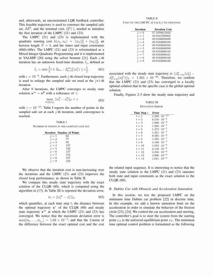
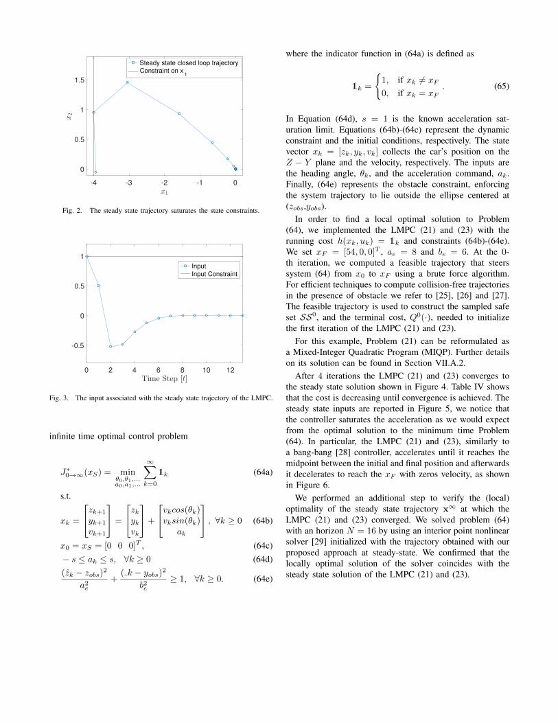
Finally, Figures 2-3 show the steady state trajectory and

TABLE IIIDEVIATION ERROR.

Time Step t Errort = 1 1.299 · 10−14

t = 2 8.516 · 10−8

t = 3 1.008 · 10−8

t = 4 1.392 · 10−7

t = 5 1.473 · 10−7

t = 6 1.231 · 10−7

t = 7 8.395 · 10−8

t = 8 1.376 · 10−7

t = 9 4.180 · 10−7

t = 10 1.043 · 10−6

t = 11 2.140 · 10−6

t = 12 3.494 · 10−6

t = 13 4.996 · 10−6

t = 14 1.641 · 10−6

the related input sequence. It is interesting to notice that thesteady state solution to the LMPC (21) and (23) saturatesboth state and input constraints as the exact solution to theCLQR (60).

B. Dubins Car with Obstacle and Acceleration Saturation

In this section, we test the proposed LMPC on theminimum time Dubins car problem [22] in discrete time.In this example, we add a known saturation limit on theacceleration in order to simulate the behavior of the frictioncircle [23], [24]. We control the car acceleration and steering.The controller’s goal is to steer the system from the startingpoint xS to the unforced equilibrium point xF . The minimumtime optimal control problem is formulated as the following

-4 -3 -2 -1 0x1

0

0.5

1

1.5

x2

Steady state closed loop trajectory

Constraint on x1

Fig. 2. The steady state trajectory saturates the state constraints.

0 2 4 6 8 10 12Time Step [t]

-0.5

0

0.5

1

Input

Input Constraint

Fig. 3. The input associated with the steady state trajectory of the LMPC.

infinite time optimal control problem

J∗0→∞(xS) = minθ0,θ1,...a0,a1,...

∞∑k=0

1k (64a)

s.t.

xk =

zk+1

yk+1

vk+1

=

zkykvk

+

vkcos(θk)vksin(θk)

ak

, ∀k ≥ 0 (64b)

x0 = xS = [0 0 0]T , (64c)− s ≤ ak ≤ s, ∀k ≥ 0 (64d)(zk − zobs)2

a2e

+( k − yobs)2

b2e≥ 1, ∀k ≥ 0. (64e)

where the indicator function in (64a) is defined as

1k =

{1, if xk 6= xF

0, if xk = xF. (65)

In Equation (64d), s = 1 is the known acceleration sat-uration limit. Equations (64b)-(64c) represent the dynamicconstraint and the initial conditions, respectively. The statevector xk = [zk, yk, vk] collects the car’s position on theZ − Y plane and the velocity, respectively. The inputs arethe heading angle, θk, and the acceleration command, ak.Finally, (64e) represents the obstacle constraint, enforcingthe system trajectory to lie outside the ellipse centered at(zobs,yobs).

In order to find a local optimal solution to Problem(64), we implemented the LMPC (21) and (23) with therunning cost h(xk, uk) = 1k and constraints (64b)-(64e).We set xF = [54, 0, 0]T , ae = 8 and be = 6. At the 0-th iteration, we computed a feasible trajectory that steerssystem (64) from x0 to xF using a brute force algorithm.For efficient techniques to compute collision-free trajectoriesin the presence of obstacle we refer to [25], [26] and [27].The feasible trajectory is used to construct the sampled safeset SS0, and the terminal cost, Q0(·), needed to initializethe first iteration of the LMPC (21) and (23).

For this example, Problem (21) can be reformulated asa Mixed-Integer Quadratic Program (MIQP). Further detailson its solution can be found in Section VII.A.2.

After 4 iterations the LMPC (21) and (23) converges tothe steady state solution shown in Figure 4. Table IV showsthat the cost is decreasing until convergence is achieved. Thesteady state inputs are reported in Figure 5, we notice thatthe controller saturates the acceleration as we would expectfrom the optimal solution to the minimum time Problem(64). In particular, the LMPC (21) and (23), similarly toa bang-bang [28] controller, accelerates until it reaches themidpoint between the initial and final position and afterwardsit decelerates to reach the xF with zeros velocity, as shownin Figure 6.

We performed an additional step to verify the (local)optimality of the steady state trajectory x∞ at which theLMPC (21) and (23) converged. We solved problem (64)with an horizon N = 16 by using an interior point nonlinearsolver [29] initialized with the trajectory obtained with ourproposed approach at steady-state. We confirmed that thelocally optimal solution of the solver coincides with thesteady state solution of the LMPC (21) and (23).

TABLE IVCOST OF THE LMCPC AT EACH j-TH ITERATION

Iteration Iteration Costj = 0 39j = 1 21j = 2 18j = 3 17j = 4 16j = 5 16

0 5 10 15 20 25 30 35 40 45 50 55

Z-axis

0

10

20

30

40

50

Y-axis

Steady State Trajectory x∞

Trajectory 0-th iteration x0

Fig. 4. Comparison between the first feasible trajectory x0 and the steadystate trajectory x∞.

0 5 10 15

Time Step [t]

-1.0

0.0

1.0

a∞ k

0 5 10 15

Time Step [t]

-0.5

0

0.5

θ∞ k

Fig. 5. The acceleration a∞k and steering θ∞k inputs associated with thesteady state trajectory x∞.

C. Dubins Car with Obstacle and Unknown AccelerationSaturation

Consider the minimum time Dubins car problem (64)presented in the previous example. We assume in this sectionthat the saturation limit s is unknown. We use a sigmoid

5 10 15

Time Step [t]

0

1

2

3

4

5

6

7

v∞ k

Fig. 6. The velocity profile v∞k of the steady state trajectory x∞.

function ak√1+a2k

as a continuously differentiable approxima-

tion of the saturation function and reformulate (64) as

J∗0→∞(xS) = minθ0,θ1,...a0,a1,...

∞∑k=0

1k (66a)

s.t.

xk =

zk+1

yk+1

vk+1

=

zkykvk

+

vkcos(θk)vksin(θk)s ak√

1+a2k

, ∀k ≥ 0 (66b)

x0 = xS = [0 0 0]T , (66c)(zk − zobs)2

a2e

+(yk − yobs)2

b2e≥ 1, ∀k ≥ 0. (66d)

where the indicator functino 1k is defined in (65). The statevector xk = [zk, yk, vk] collects the car position of car onthe Z-Y plane and the velocity, respectively. The inputsare the acceleration ak and the heading angle θk. Finally, srepresents the unknown saturation limit. As in the previousexample, we set xF = [54, 0, 0]T , ae = 8 and be = 6. Thevehicle model uses a saturation limit s = 1. This is unknownto the controller.

We apply the proposed LMPC on an augmented systemto simultaneously estimated the saturation coefficient and tosteer the system (66b) to the terminal point xF . In order toarchive this, we define a saturation coefficient estimate, sk,and an error estimate ek = s− sk. The idea of augmentingthe system with an estimator and a related error dynamicsis standard in adaptive control strategies [30] [31]. Theobjective of the controller is a trade off between estimatingthe saturation coefficient and steering the system to theterminal point xF . The LMPC solves at time t of the j-th

iteration the following problem,

J LMPC,j0→N (xjt ) = min

θ0,...,θNa0,...,aNδ0,...,θN

[N−1∑k=0

wee2k + 1k

]+Qj−1(xN )

(67a)s.t.

xk+1 =f(xk, uk) =

zkykvkskek

+

vkcos(θk)vksin(θk)sk+1

ak√1+a2k

δk−δk

, ∀k ≥ 0

(67b)

x0 = xjt , (67c)(zk − zobs)2

a2e

+(yk − yobs)2

b2e≥ 1, ∀k ≥ 0, (67d)

xN ∈ SSj−1, (67e)

where N = 4 and the weight on the error estimate we = 10.The indicator function 1k in (67a) is defined as

1k =

{1, if xk /∈ XF0, if xk ∈ XF

. (68)

where

XF =

{x =

zyvse

∈ R5 :

zyv

= xF , s ∈ R, e = 0

}. (69)

f(·, ·) in (67b) represents the dynamics updateof the augmented system and the state vectorxk = [zk, yk, vk, sk, ek] collects the estimate position onthe Z-Y plane, the car’s velocity, the saturation coefficientestimator and the estimator error, respectively. The inputvector uk = [ak, θk, δk] collects the acceleration, the steeringand the estimate difference between two consecutive timesteps, respectively. Equation (67c) represents the initialcondition and (67d) the obstacle avoidance constraint.Constraint (67e) enforces the terminal state into the SSj−1

defined in equation (12). Finally, in (67) we have used asimplified notation to equation (21).Let at time t of the j-th iteration u∗,jt:t+N |t be the optimalsolution to (67), then we apply the first element of u∗,jt:t+N |tto the system in (67b)

ujt = u∗,jt|t . (70)

We assume that at time t of the j-th iteration the system statexjt = [zjt , y

jt , v

jt ] is measured and we estimate ejt inverting

the system dynamics (66b) and (67b)

ejt =

yjt−y

jt−(yjt−1−y

jt-1)

ajt−1√

1+(ajt−1

)2

, If at−1√1+a2t−1

6= 0

ejt−1 otherwise

. (71)

Remark 9: Consider a local optimal solutionx∗ = [z∗, y∗, v∗, s∗, e∗]T to problem (67) definedover the infinite horizon. If e∗k = 0, ∀k > 0, (i.e., thealgorithm has successfully identified the friction saturationcoefficient), then x∗ = [z∗, y∗, v∗] is a local optimalsolution for the original problem (64).

Initialization of the LMPC (67) is discussed in the Ap-pendix. For this example, Problem (21) can be reformulatedas a Mixed-Integer Quadratic Program (MIQP). Furtherdetails on its solution can be found in Section VII.A.2.

After 7 iterations, the LMPC (67), (70) converges to asteady state solution. Figure 8 illustrates the evolution ofthe sampled safe set through the iterations and Table Vshows that the iteration cost is decreasing until convergenceis reached.

1 2 3 4 5 6 7 8 9

Iteration [j]

0

0.05

0.1

0.15

0.2

0.25

0.3

0.35

0.4

0.45

||ej 1:tj||1

Fig. 7. Evolution of the 1-norm of the estimation error through theiterations.

Figure 7 shows the behavior of the 1-norm of the errorvector

ej1:∞ = [ej1, . . . , ejt , . . . ]. (72)

as a function of the iteration j. We notice that the LMPC(67), (70) correctly learns from the previous iterations de-creasing the estimation error, until it identifies the unknownsaturation coefficient (i.e. e∞k = 0 ∀k > 0).

0 5 10 15 20 25 30 35 40 45 50 55

Z-axis

0

10

20

30

40

50

Y-axis

Sampled safe set at the 1st iterations

0 5 10 15 20 25 30 35 40 45 50 55

Z-axis

0

10

20

30

40

50

Y-axis

Sampled safe set at the 2nd iterations

0 5 10 15 20 25 30 35 40 45 50 55

Z-axis

0

10

20

30

40

50

Y-axis

Sampled safe set at the 5th iterations

0 5 10 15 20 25 30 35 40 45 50 55

Z-axis

0

10

20

30

40

50

Y-axis

Sampled safe set at steady state

Fig. 8. Sampled safe set evolution over the iterations.

0 5 10 15

Time Step [t]

-1.0

0.0

1.0

a∞ k

0 5 10 15

Time Step [t]

-0.5

0

0.5

θ∞ k

Fig. 9. The acceleration a∞k and steering θ∞k inputs associated with thesteady state trajectory x∞.

The steady state inputs are reported in Figure 9. One canobserve that the LMPC (67), (70) saturates the accelerationconstraints. The controller accelerates until it reaches the

0 5 10 15 20 25 30 35 40 45 50 55

Z-axis

0

10

20

30

40

50

Y-axis

Steady State Trajectory x∞

Trajectory 0-th iteration x0

Fig. 10. Steady state trajectory of the LMPC on the Z − Y plane.

midpoint between the initial and final position and it de-celerates afterwards, as we would expect from the optimalsolution to a minimum time problem [28]. Figure 10 showsthe steady state trajectory x∞, and the feasible trajectory

x0 at the 0-th iteration. The LMPC (67) and (70) steers thesystem from the staring point xS to the final point xF in 16steps as the optimal solution to (64) computed in the previousexample.

TABLE VOPTIMAL COST OF THE LMPC AT EACH j-TH ITERATION

Iteration Iteration Costj = 0 65.000000000000000j = 1 33.634529488066327j = 2 24.216166714512450j = 3 19.625000000001727j = 4 19.625000000000004j = 5 17.625000000022546j = 6 17.625000000000000j = 7 16.625000000000000j = 8 16.625000000000000

V. PRACTICAL CONSIDERATIONS

A. Computation

The sampled safe set (12) is a set of discrete pointsand therefore the terminal constraint in (21e) is aninteger constraint. Consequently, the proposed approachis computationally expensive also for linear system asthe controller has to solve a mixed integer programmingproblem at each time step. In the following we discuss twodifferent approaches to improve the computational burdenassociated with the proposed control logic.

1) Convexifing the terminal constraint: Thecomputational burden associated with the finite timeoptimal control problem (21) can be reduced relaxing thesampled safe to its convex hull, and the Q(·) functionto be its barycentric approximation. For more details onbarycentric approximation we refer to [17]. This relaxedproblem is convex if the system dynamics is linear andthe stage cost is convex. Furthermore, for linear systemand convex stage cost, the relaxed approach preserves theproperties showed in Theorems 1-3 of [32]. When thesystem is nonlinear, it is still possible to apply the convexrelaxation but guarantees are, in general, lost. In [33], thisrelaxed approach has been successfully applied in real timeto the nonlinear minimum time autonomous racing problem,where the LMPC is used to improve the vehicle’s lap timeover the iterations. A video of a more recent implementationon the Berkeley Autonomous Racing Car (BARC) platformcan be found here: https://automatedcars.space/home/

2016/12/22/learning-mpc-for-autonomous-racing .

2) Parallelize Computations: The structure of the LMPCcan be exploited to design an algorithm that: i) use a subsetof the sampled safe in the (21), ii) can be parallelized. Inparticular, one can compute an upper and lower bound tothe optimal solution of problem (21). These bounds allow toreduce the complexity of (21) without loosing the guaranteesproven in Theorems 1-3. More details are discussed next.

First, we notice that at time t, ∀t > 0 it is possible tocompute an upper bound on the optimal cost of problem(21), using the solution computed at time t−1. In particular,from equations (6) and (33) we have,

J LMPC,j0→N (xjt )− J

LMPC,j0→N (xjt−1) ≤ −h(xjt−1, u

jt−1) ≤ 0, (73)

which implies that at time t an upper bound on the optimalcost is given by

J LMPC,j0→N (xjt ) ≤ J

LMPC,j0→N (xjt−1). (74)

In order to compute a lower bound, let (22) be the optimalsolution to (21), then at the j-th iteration

J LMPC,jt→t+N (xjt ) =

t+N−1∑k=t

h(x∗,jk|t , u∗,jk|t) +Qj−1(x∗,jt+N |t). (75)

As Problem (67) is time-invariant and h(·, ·) is positivedefinite (6), we have

J LMPC,j0→N (xjt ) ≥ Qj−1(x∗,jt+N |t), ∀x

∗,jt+N |t ∈ SS

j−1. (76)

Combining the upper bound (74) and the lower bound (76),we obtain

Qj−1(x∗,jt+N |t) ≤ JLMPC,j0→N (xjt ) ≤ J

LMPC,j0→N (xjt−1). (77)

Therefore at optimum we have that

Qj−1(x∗,jt+N |t) ≤ JLMPC,j0→N (xjt−1). (78)

Define RSj−1t as the set of points which satisfy condition

(78),

RSj−1t = {x ∈ SSj−1

t : Qj−1(x) ≤ J LMPC,j0→N (xjt−1)}, (79)

then, from equation (78), we deduce that for t > 0

x∗,jt+N |t ∈ RSj−1t ⊆ SSj−1. (80)

The set RS can be used in place of SS in order to reducecomputational complexity.

The following Algorithm 1 uses this idea to solve theLMPC (21), (23). Algorithm 1 was used for the Dubins Carexample with the nonlinear solver Ipopt [29].

Algorithm 1: Compute ujt at time t of the j-th iteration

Read measurements and update xjt and t.if t > 0 then

Compute RSj−1t

elseSet RSj−1

t = SSj−1

endn = 0for all x ∈ RSj−1

t doIn (21), set SSj−1 = xSolve (21) using a nonlinear optimization solver.Set un = u∗,jt|t and Jn = J LMPC,j

t→t+N (xjt )n = n+ 1

endFind n∗ = arg minn JnApply ujt = un∗

B. Uncertainty

The paper uses a deterministic framework and the the-oretical guaranties have been demonstrated only for thedeterministic case. This is the case of the vast majority ofseminal papers on MPC [16], [34], [35], [36]. In the presenceof disturbances, as for all deterministic MPC schemes, all theguarantees are lost. However, one can build on the proposedresults to formulate a stochastic iterative learning MPC. Forinstance if disturbance is modeled as a Gaussian process thechance constraint can be converted to deterministic secondorder cone constraint [37], which can be handled with theproposed control logic. Furthermore, the proposed controllogic can be extended to a robust iterative learning MPCwhen the disturbance is bounded and the system is linear.Under these assumptions the robust MPC can be formulatedin a deterministic control problem tightening the constraints[38]. In particular, the robust MPC can be designed on anominal model where the tightening of the state constraintsis computed to guarantee that the original system satisfiesthe nominal constraints for all the disturbance values [38].This is topic of further investigation.

VI. CONCLUSIONS

In this paper, a reference-free learning nonlinear modelpredictive control that exploits information from the previousiterations to improve the performance of the closed loopsystem over iterations is presented. A safe set and a terminalcost, learnt from previous iterations, allow to guarantee therecursive feasibility and stability of the closed loop system.Moreover, we showed that if the closed-loop system con-verges to steady state trajectory then this trajectory is locally

optimal for the infinite horizon optimal control problem,regardless of the LMPC optimization horizon. We testedthe proposed control logic on an infinite horizon linearquadratic regulator with constraints (CLQR) to shown thatthe proposed control logic converges to the optimal solutionof the infinite optimal control problem. Finally, we tested thecontrol logic on nonlinear minimum time problem optimalcontrol problem and we showed that the properties of theproposed LMPC can be used to simultaneously estimateunknown system parameters and to generate a state trajectorythat pushes system performance.

VII. ACKNOWLEDGMENTS

We thank the reviews for their feedback on the manuscript.

VIII. APPENDIX

In order to compute a feasible trajectory that steers system(67b) from the initial state x0 = [x0, s0, e0]T into XF weused a greedy approach described next. First, we set δk =0, ∀k = 1, · · · , N − 1. Therefore, from (67b), we have that

sk = s0, ∀k = 1, · · · , N − 1 (81a)ek = e0, ∀k = 1, · · · , N − 1. (81b)

Afterwards, we selected an initial guess for the saturationcoefficient estimate s0 = 0.25 and given the following inputstructure

θk = θ, ∀k = 1, · · · , Ns (82a)

θk = −θ, ∀k = Ns + 1, · · · , N − 1 (82b)ak = a, ∀k = 1, · · · , Ns (82c)ak = 0, ∀k = Ns + 1, · · · , N − Ns (82d)

aN−1 = −a, ∀k = N − Ns + 1, · · · , N (82e)

we generated a set of trajectories using different sets of pa-rameters θ, Ns, Ns, a, N . Among the generated trajectories,we used the one minimizing the following quantity

||

zN−1

yN−1

vN−1

sN−1

eN−1

− xFsN−1

eN−1

||22 (83)

to warm-start a nonlinear optimization problem which al-lowed us to find the following N − 1 step trajectory

x00:N−1 =

[x0

0, · · · , x0N−1 =

xFsN−1

eN−1

], (84)

and the related input sequence

(θ0k, a

0k), ∀k = 1, · · · , N − 1. (85)

Afterwards the input sequence (85) are applied to the system(64b) to compute

x00:N−1 = [x0

0, · · · , x0N−1]. (86)

Then realized trajectories x00:N−1 and x0

0:N−1 are used tocompute the error, which from equations (64b) and (67b), isgiven by

ek+1 =

yk+1−yk+1−(yk−yk)

ak√1+a2

k

, If ak√1+a2k

6= 0

ek else(87)

∀k = 0, · · · , N − 2.Finally, we selected

θ0N = a0

N = 0 (88a)

δ0N = eN−1 (88b)

to regulate e0N−1 to zero steering x0

N−1 into XF . Concluding,the N steps trajectory which extends the trajectory in (84)using (88),

x00:N =

[x0

0, · · · , x0N =

xFsN0

] (89)

steers system (67b) into XF and it can be used to build SS0

and Q0(·).

REFERENCES

[1] D. A. Bristow, M. Tharayil, and A. G. Alleyne, “A survey of iterativelearning control,” IEEE Control Systems, vol. 26, no. 3, pp. 96–114,2006.

[2] K. S. Lee and J. H. Lee, “Model predictive control for nonlinearbatch processes with asymptotically perfect tracking,” Computers &Chemical Engineering, vol. 21, pp. S873–S879, 1997.

[3] J. H. Lee and K. S. Lee, “Iterative learning control applied tobatch processes: An overview,” Control Engineering Practice, vol. 15,no. 10, pp. 1306–1318, 2007.

[4] Y. Wang, F. Gao, and F. J. Doyle, “Survey on iterative learning control,repetitive control, and run-to-run control,” Journal of Process Control,vol. 19, no. 10, pp. 1589–1600, 2009.

[5] C.-Y. Lin, L. Sun, and M. Tomizuka, “Matrix factorization for designof q-filter in iterative learning control,” in 2015 54th IEEE Conferenceon Decision and Control (CDC). IEEE, 2015, pp. 6076–6082.

[6] ——, “Robust principal component analysis for iterative learningcontrol of precision motion systems with non-repetitive disturbances,”in 2015 American Control Conference (ACC). IEEE, 2015, pp. 2819–2824.

[7] K. S. Lee, I.-S. Chin, H. J. Lee, and J. H. Lee, “Model predictive con-trol technique combined with iterative learning for batch processes,”AIChE Journal, vol. 45, no. 10, pp. 2175–2187, 1999.

[8] K. S. Lee and J. H. Lee, “Convergence of constrained model-basedpredictive control for batch processes,” IEEE Transactions on Auto-matic Control, vol. 45, no. 10, pp. 1928–1932, 2000.

[9] J. H. Lee, K. S. Lee, and W. C. Kim, “Model-based iterative learningcontrol with a quadratic criterion for time-varying linear systems,”Automatica, vol. 36, no. 5, pp. 641–657, 2000.

[10] J. R. Cueli and C. Bordons, “Iterative nonlinear model predictivecontrol. stability, robustness and applications,” Control EngineeringPractice, vol. 16, no. 9, pp. 1023–1034, 2008.

[11] R. Sharp and H. Peng, “Vehicle dynamics applications of optimalcontrol theory,” Vehicle System Dynamics, vol. 49, no. 7, pp. 1073–1111, 2011.

[12] A. Rucco, G. Notarstefano, and J. Hauser, “An efficient minimum-time trajectory generation strategy for two-track car vehicles,” IEEETransactions on Control Systems Technology, vol. 23, no. 4, pp. 1505–1519, 2015.

[13] Y.-L. Hwang, T.-N. Ta, C.-H. Chen, and K.-N. Chen, “Using zeromoment point preview control formulation to generate nonlinear trajec-tories of walking patterns on humanoid robots,” in Fuzzy Systems andKnowledge Discovery (FSKD), 2015 12th International Conferenceon. IEEE, 2015, pp. 2405–2411.

[14] S. Kuindersma, F. Permenter, and R. Tedrake, “An efficiently solvablequadratic program for stabilizing dynamic locomotion,” in 2014 IEEEInternational Conference on Robotics and Automation (ICRA). IEEE,2014, pp. 2589–2594.

[15] C. E. Garcia, D. M. Prett, and M. Morari, “Model predictive control:theory and practice a survey,” Automatica, vol. 25, no. 3, pp. 335–348,1989.

[16] D. Q. Mayne, J. B. Rawlings, C. V. Rao, and P. O. Scokaert,“Constrained model predictive control: Stability and optimality,” Au-tomatica, vol. 36, no. 6, pp. 789–814, 2000.

[17] F. Borrelli, Constrained optimal control of linear and hybrid systems.Springer, 2003, vol. 290.

[18] E. G. Gilbert and K. T. Tan, “Linear systems with state and controlconstraints: The theory and application of maximal output admissiblesets,” IEEE Transactions on Automatic control, vol. 36, no. 9, pp.1008–1020, 1991.

[19] D. P. Bertsekas, Dynamic programming and optimal control. AthenaScientific Belmont, MA, 1995, vol. 1, no. 2.

[20] J. Lofberg, “Yalmip: A toolbox for modeling and optimization inmatlab,” in Computer Aided Control Systems Design, 2004 IEEEInternational Symposium on. IEEE, 2004, pp. 284–289.

[21] P. Bonami, L. T. Biegler, A. R. Conn, G. Cornuejols, I. E. Grossmann,C. D. Laird, J. Lee, A. Lodi, F. Margot, N. Sawaya et al., “Analgorithmic framework for convex mixed integer nonlinear programs,”Discrete Optimization, vol. 5, no. 2, pp. 186–204, 2008.

[22] L. E. Dubins, “On curves of minimal length with a constraint onaverage curvature, and with prescribed initial and terminal positionsand tangents,” American Journal of mathematics, vol. 79, no. 3, pp.497–516, 1957.

[23] Y. Gao, T. Lin, F. Borrelli, E. Tseng, and D. Hrovat, “Predictive controlof autonomous ground vehicles with obstacle avoidance on slipperyroads,” in ASME 2010 dynamic systems and control conference.American Society of Mechanical Engineers, 2010, pp. 265–272.

[24] R. Rajamani, Vehicle dynamics and control. Springer Science &Business Media, 2011.

[25] F. Bullo, E. Frazzoli, M. Pavone, K. Savla, and S. L. Smith, “Dynamicvehicle routing for robotic systems,” Proceedings of the IEEE, vol. 99,no. 9, pp. 1482–1504, 2011.

[26] Y. Kuwata, G. A. Fiore, J. Teo, E. Frazzoli, and J. P. How, “Motionplanning for urban driving using rrt,” in Intelligent Robots and Systems,2008. IROS 2008. IEEE/RSJ International Conference on. IEEE,2008, pp. 1681–1686.

[27] S. Karaman and E. Frazzoli, “Incremental sampling-based algorithmsfor optimal motion planning,” Robotics Science and Systems VI, vol.104, 2010.

[28] D. Liberzon, Calculus of variations and optimal control theory: aconcise introduction. Princeton University Press, 2012.

[29] H. Pirnay, R. Lopez-Negrete, and L. T. Biegler, “Optimal sensitivitybased on ipopt,” Mathematical Programming Computation, vol. 4,no. 4, pp. 307–331, 2012.

[30] H. Bai, M. Arcak, and J. T. Wen, “Adaptive motion coordination:Using relative velocity feedback to track a reference velocity,” Auto-matica, vol. 45, no. 4, pp. 1020–1025, 2009.

[31] G. C. Goodwin, R. L. Leal, D. Q. Mayne, and R. H. Middleton,“Rapprochement between continuous and discrete model referenceadaptive control,” Automatica, vol. 22, no. 2, pp. 199–207, 1986.

[32] U. Rosolia and F. Borrelli, “Learning Model Predictive Control forIterative Tasks: A Computationally Efficient Approach for LinearSystem,” ArXiv e-prints, Feb. 2017.

[33] U. Rosolia, A. Carvalho, and F. Borrelli, “Autonomous Racing usingLearning Model Predictive Control,” ArXiv e-prints, Oct. 2016.

[34] A. Zheng and M. Morari, “Stability of model predictive control withmixed constraints,” IEEE Transactions on Automatic Control, vol. 40,no. 10, pp. 1818–1823, 1995.

[35] C. E. Garcia, D. M. Prett, and M. Morari, “Model predictive control:theory and practicea survey,” Automatica, vol. 25, no. 3, pp. 335–348,1989.

[36] S. L. de Oliveira Kothare and M. Morari, “Contractive model predic-tive control for constrained nonlinear systems,” IEEE Transactions onAutomatic Control, vol. 45, no. 6, pp. 1053–1071, 2000.

[37] G. C. Calafiore and L. El Ghaoui, “Linear programming with prob-ability constraints-part 1,” in American Control Conference, 2007.ACC’07. IEEE, 2007, pp. 2636–2641.

[38] B. Kouvaritakis and M. Cannon, Model Predictive Control: Classical,Robust and Stochastic. Springer, 2015.

Ugo Rosolia received the B.S. and M.S. (cumlaude) degrees in mechanical engineering from thePolitecnico di Milano, Milan, Italy, in 2012 and2014, respectively. He is currently pursuing thePh.D. degree in mechanical engineering with theUniversity of California at Berkeley, Berkeley, CA,USA.

He was a Visiting Scholar with Tongji Uni-versity, Shanghai, China, for the Double DegreeProgram PoliTong from 2010 to 2011. During hisM.S. degree, he was a Visiting Student for two

semesters with the University of Illinois at Urbana-Champaign, Urbana, IL,USA, sponsored by a Global E3 Scholarship. He was a Research Engineerwith Siemens PLM Software, Leuven, Belgium, in 2015, where he wasinvolved in the optimal control algorithms. His current research interestsinclude nonlinear optimal control for the centralized and decentralizedsystem, the iterative learning control, and the predictive control.

Francesco Borrelli received the Laurea degree incomputer science engineering from the Universityof Naples Federico II, Naples, Italy, in 1998,and the Ph.D. degree from ETH-Zurich, Zurich,Switzerland, in 2002.

He is currently an Associate Professor withthe Department of Mechanical Engineering, Uni-versity of California, Berkeley, CA, USA. Heis the author of more than 100 publications inthe field of predictive control and author of thebook Constrained Optimal Control of Linear and

Hybrid Systems (Springer Verlag). His research interests include constrainedoptimal control, model predictive control and its application to advancedautomotive control and energy efficient building operation.

Dr. Borrelli was the recipient of the 2009 National Science FoundationCAREER Award and the 2012 IEEE Control System Technology Award.In 2008, he was appointed the chair of the IEEE technical committee onautomotive control.