J Dyn Diff EquatDOI 10.1007/s10884-009-9153-6

A General Approach for Front-Propagation in FunctionalReaction-Diffusion Equations

Alessandro Calamai · Cristina Marcelli ·Francesca Papalini

Received: 13 March 2008 / Revised: 9 June 2009© Springer Science+Business Media, LLC 2009

Abstract We investigate the persistence of front propagation for functional reaction-diffusion equations

vτ = vxx + F(v)

where F is a given operator. By combining the upper and lower solution method with fixedpoint techniques, we prove a general existence theorem for traveling waves. Our result appliesto reaction-diffusion equation with delayed or non-local reaction term.

Keywords Delayed reaction-diffusion equations · Non-local reaction-diffusion equations ·Traveling waves · Monostable reaction-term · Upper and lower-solutions method ·Fixed point

Mathematics Subject Classification (2000) 35K57 · 34K10 · 35B40 · 35R10

1 Introduction

The study of the existence and qualitative properties of traveling fronts for reaction-diffusionequations is a widely investigated field of research, due to several applications in variousbiological phenomena (see e.g. [14]). The usual Fisher–KPP equation modeling a reaction-diffusion process (see [4,10]) is

A. Calamai · C. Marcelli · F. Papalini (B)Dipartimento di Scienze Matematiche, Università Politecnica delle Marche, Via Brecce Bianche,60131 Ancona, Italye-mail: papalini@dipmat.univpm.it

A. Calamaie-mail: calamai@dipmat.univpm.it

C. Marcellie-mail: marcelli@dipmat.univpm.it

123

J Dyn Diff Equat

vτ = vxx + f (v), τ ≥ 0, x ∈ R

where f ∈ C1[0, 1] satisfies f (0) = f (1) = 0, f (v) > 0 in (0, 1). The study of travelingwave solutions (t.w.s.) connecting the stationary states 0 and 1 has a great relevance in theinvestigation of the asymptotic behavior (for τ large) of a generic solution of the associatedinitial value problem since it is known that in certain cases the solution evolves (in somesense) towards the t.w.s. having minimal speed (see [9]). More in detail, a t.w.s. is a solutionof the equation having a constant profile: v(τ, x) = u(x − cτ) for some function u ∈ C2(R)

(the wave profile) and constant c (the wave speed). It is well-known that each t.w.s. is mono-tone, and that there is a threshold value c∗ such that there exist fronts having speed c ifand only if c ≥ c∗ and the stable t.w.s. corresponds to the minimal speed c∗. This value isunknown in general, but the following estimate holds (see, e.g., [1]):

2√

f ′(0) ≤ c∗ ≤ 2

√

supu∈(0,1]

f (u)

u.

Of course, when f is concave, the inequalities in the previous formula are actually equalitiesand c∗ = 2

√f ′(0). The research in this field has been carried out also for equations having

non-constant diffusivity or in the presence of a convective term. We refer to the monographs[3,5,14,16] and references therein contained.

Recently, some models of non-local reaction-diffusion equations have been proposed byGourley (see [6]), in which the reaction term contains a convolution integral

vτ = vxx + v(τ, x)

⎛

⎝1 −+∞∫

−∞�(x − y)v(τ, y) dy

⎞

⎠

where the kernel� is even, non-negative, summable in R with unitary integral (normalized).The classical local Fisher equation (with f (v) = v(1 − v)) can be considered as a particularcase, arising when the kernel � is the Dirac delta function.

In this setting the non-local term has the meaning of a weighted average of the density vand models interactions between individuals competing not only with those localized at theirown point, but also with individuals in other points of the domain. A prototype kernel is theso-called Laplace exponential distribution

�(ξ) := b

2e−b|ξ |, b > 0

naturally arising from the model of the consumption of resources. Note that for large val-ues of b the interaction is strong with close points, so the value 1

b can be considered as ameasure of the non-locality (see [6]). To the best of our knowledge, no rigorous analysis isavailable for such equations. Actually, in [6] an approximate model has been investigatedfrom a qualitative point of view.

Another field having an increasing interest, is that of reaction-diffusion equations or sys-tems with time-delay, in which the reaction term also depends on v(τ − T, x). In this areaseveral results have been obtained, but mainly for specific forms of the reaction term (see,e.g., [2,7,8,17]). Moreover, some of the most recent ones present some problematic aspect(see Remark 4.2).

The aim of the present paper is to propose a general unifying approach for dealing withfunctional reaction-diffusion equations, including both the non-local equations and the de-layed ones, and to enlarge the class of reaction terms to which one can apply the general

123

J Dyn Diff Equat

existence result. More precisely, we consider the following general boundary value problem{

u′′ + cu′ + F(u) = 0u(−∞) = 1, u(+∞) = 0

where F : C(R) → C(R) is a given functional operator. Assuming the existence of a pairof well-ordered upper and lower-solutions, we prove a general existence result (see Theo-rem 4.3). Moreover, we show how it can be applied to reaction-diffusion equations havingnon-local or delayed terms, showing that under certain limitations on the wave speed c, apair of upper and lower-solutions can be actually found (see Theorems 5.2, 5.3, 5.7).

In particular, our existence result can be fruitfully applied to delayed reaction-diffusionequation of the type

vτ (τ, x) = vxx (τ, x)+ g(v(τ, x))v(τ − T, x)

or non-local equations of the type

vτ (τ, x) = vxx (τ, x)+ g(v(τ, x))

+∞∫

−∞�(x − σ)v(τ, σ ) dσ,

where g is a generic Lipschitz function satisfying

0 < g(u) ≤ g(0)(1 − u) for every u ∈ [0, 1).

We underline that both in the non-local setting and in the delayed one, we obtain the exis-tence of t.w.s. when the speed c lies in a certain interval [c∗

1, c∗2]. We show that in both cases,

when the model tends to the usual Fisher–KPP one, for instance when the delay tends to 0 orthe kernel in the non-local equation tends to the Dirac delta function, then the left endpointc∗

1 tends to the threshold value c∗ of the non-functional equation and the right endpoint c∗2

diverges to +∞.Our approach is based on fixed point techniques combined to the method of upper and

lower-solutions, following an idea considered by Ma in [11] (see Sect. 2). In Sects. 3 and 4,we present general existence results, which are applied to non-local or delayed equations inSect. 5. Finally, in Sect. 6, we discuss the results and the open problems.

2 An Auxiliary Problem

This section is devoted to some preliminary results related to an auxiliary linear problem.Let c ∈ R, β > 0 be fixed. Given h ∈ L∞(R), in what follows we will consider the

function uh : R → R defined by

uh(t) := −eα1t

t∫

−∞h(s)e−α1s ds − eα2t

+∞∫

t

h(s)e−α2s ds, t ∈ R, (2.1)

where α1 < 0 < α2 are the solutions of the algebraic equation x2 + cx − β = 0.The following result concerns some properties of the function uh .

Lemma 2.1 Let h ∈ L∞(R). Then

(i) uh is a C1-function on R, with u′h a.e. differentiable, and

u′′h(t)+ cu′

h(t)− βuh(t) = (α2 − α1)h(t) for a.e. t ∈ R;

123

J Dyn Diff Equat

(ii) if h(t) ≤ 0 for a.e. t ∈ R, then uh(t) ≥ 0 for every t ∈ R.(iii) if −β ≤ h(t) ≤ 0 for a.e. t ∈ R, then 0 ≤ uh(t) ≤ α2 −α1 and |u′

h(t)| ≤ 2β for everyt ∈ R;

(iv) if h is monotone increasing, then uh is monotone decreasing.(v) if h is continuous for |t | large and if h(±∞) exist, then uh(±∞) exist too and

uh(±∞) = −h(±∞) α2−α1β

.

Proof First observe that uh is absolutely continuous on every compact interval of R, henceit is differentiable for a.e. t ∈ R with

u′h(t) = −α1eα1t

t∫

−∞h(s)e−α1s ds − α2eα2t

+∞∫

t

h(s)e−α2s ds a.e. t ∈ R. (2.2)

The right-hand side of (2.2) is a continuous function on R, call it γ (t). So, since uh isabsolutely continuous in every compact interval, fixed t ∈ R we have uh(t) = uh(0) +∫ t

0 u′h(s)ds = uh(0) + ∫ t

0 γ (s)ds hence uh ∈ C1(R) and (2.2) holds for every t ∈ R.Therefore, u′

h is absolutely continuous in every compact interval and

u′′h(t) = −α2

1eα1t

t∫

−∞h(s)e−α1s ds − α2

2eα2t

+∞∫

t

h(s)e−α2s ds + (α2 − α1)h(t) a.e. t ∈ R.

Recalling that α1 and α2 satisfy the equation x2 + cx − β = 0, one gets u′′h(t) + cu′

h(t) −βuh(t) = (α2 − α1)h(t) for a.e. t ∈ R, and assertion (i) is proved.

Property (ii) is immediate. Let us prove (iii). If h(t) ≥ −β for a.e. t ∈ R, then for everyt ∈ R we have

uh(t) ≤ β

⎛

⎝eα1t

t∫

−∞e−α1sds + eα2t

+∞∫

t

e−α2sds

⎞

⎠ = β

(− 1

α1+ 1

α2

)= α2 − α1

(recall that α1α2 = −β). Furthermore, if −β ≤ h(t) ≤ 0 for a.e. t ∈ R, recalling thatα1 < 0 < α2, we have

|u′h(t)| ≤ β

⎛

⎝α2eα2t

+∞∫

t

e−α2s ds − α1eα1t

t∫

−∞e−α1s ds

⎞

⎠ = 2β for every t ∈ R.

As for property (iv), let us fix T > 0 and observe that

uh(t + T ) = −eα1t

t+T∫

−∞h(s)e−α1(s−T ) ds − eα2t

+∞∫

t+T

h(s)e−α2(s−T ) ds

= −eα1t

t∫

−∞h(σ + T ) e−α1σ dσ − eα2t

+∞∫

t

h(σ + T ) e−α2σ dσ.

with σ = s − T . Thus,

uh(t+T )−uh(t) = −eα1t

t∫

−∞(h(s+T )−h(s)) e−α1sds−eα2t

+∞∫

t

(h(s+T )− h(s)) e−α2sds.

123

J Dyn Diff Equat

Hence, if h is increasing, then h(s + T ) − h(s) ≥ 0 a.e. s ∈ R and consequently uh(t +T )− uh(t) ≤ 0 for any t ∈ R, i.e. uh is decreasing.

Finally, let us prove (v). By the L’Hopital rule,

limt→±∞ uh(t)= lim

t→±∞

(h(t)e−α1t

α1e−α1t− h(t)e−α2t

α2e−α2t

)=h(±∞)

(1

α1− 1

α2

)=h(±∞)

α2 − α1

−β .

�

Let BC(R) denote the space of all bounded continuous maps u : R → R. For everyρ > 0, we can introduce a norm ‖ · ‖ρ in the space BC(R) by defining

‖u‖ρ := supt∈R

|u(t)|e−ρ|t | < +∞. (2.3)

From now on, BCρ(R) will denote the space BC(R) endowed with the norm ‖ · ‖ρ . As it iseasy to check, BCρ(R) is a Banach space.

Let us define the linear operator S in BCρ(R) by

S(h)(t) = 1

α2 − α1uh(t), t ∈ R,

where uh was defined in (2.1).By virtue of property (iii) of Lemma 2.1, if h(t) ∈ [−β, 0] for every t ∈ R, then 0 ≤

S(h)(t) ≤ 1 for every t ∈ R. Moreover, from the linearity of S and property (ii) of thesame Lemma we conclude that S is monotone decreasing with respect the partial orderingin BC(R) induced by the cone K := {h ∈ BC(R) : h(t) ≥ 0 for every t ∈ R}, i.e.

h1(t) ≤ h2(t) for every t ∈ R ⇒ S(h1)(t) ≥ S(h2(t)) for every t ∈ R. (2.4)

Finally, from property (i) of Lemma 2.1, it follows that S(h) is a solution of the followingsecond order linear differential equation:

u′′(t)+ cu′(t)− βu(t) = h(t), a.e. t ∈ R. (2.5)

The next Lemma states that S is continuous with respect to the norm ‖ · ‖ρ for ρ > 0small enough.

Lemma 2.2 The operator S is continuous in BCρ(R) for every ρ < min{−α1, α2}. Moreprecisely, there exists a constant k = k(ρ) such that

‖S(h1)− S(h2)‖ρ ≤ k‖h1 − h2‖ρ for every h1, h2 ∈ BC(R). (2.6)

123

J Dyn Diff Equat

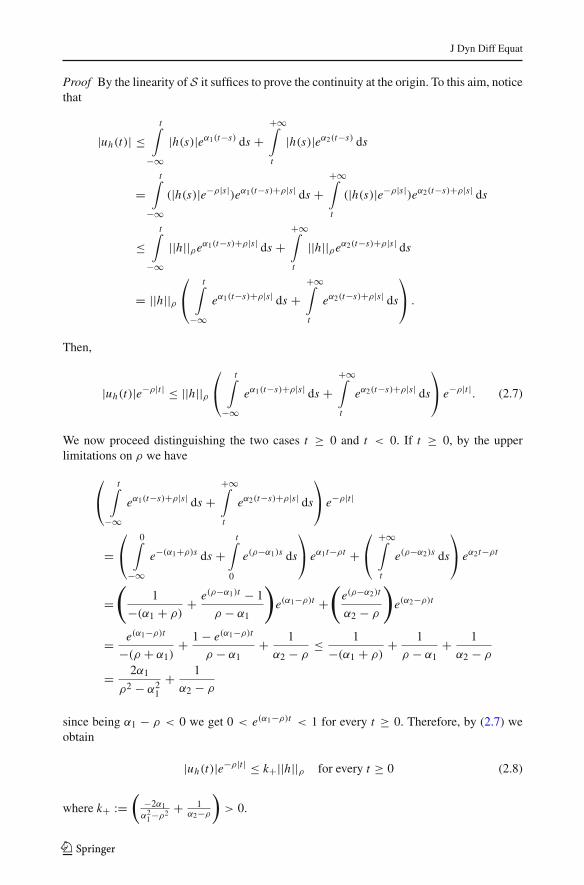
Proof By the linearity of S it suffices to prove the continuity at the origin. To this aim, noticethat

|uh(t)| ≤t∫

−∞|h(s)|eα1(t−s) ds +

+∞∫

t

|h(s)|eα2(t−s) ds

=t∫

−∞(|h(s)|e−ρ|s|)eα1(t−s)+ρ|s| ds +

+∞∫

t

(|h(s)|e−ρ|s|)eα2(t−s)+ρ|s| ds

≤t∫

−∞||h||ρeα1(t−s)+ρ|s| ds +

+∞∫

t

||h||ρeα2(t−s)+ρ|s| ds

= ||h||ρ⎛

⎝t∫

−∞eα1(t−s)+ρ|s| ds +

+∞∫

t

eα2(t−s)+ρ|s| ds

⎞

⎠ .

Then,

|uh(t)|e−ρ|t | ≤ ||h||ρ⎛

⎝t∫

−∞eα1(t−s)+ρ|s| ds +

+∞∫

t

eα2(t−s)+ρ|s| ds

⎞

⎠ e−ρ|t |. (2.7)

We now proceed distinguishing the two cases t ≥ 0 and t < 0. If t ≥ 0, by the upperlimitations on ρ we have

⎛

⎝t∫

−∞eα1(t−s)+ρ|s| ds +

+∞∫

t

eα2(t−s)+ρ|s| ds

⎞

⎠ e−ρ|t |

=⎛

⎝0∫

−∞e−(α1+ρ)s ds +

t∫

0

e(ρ−α1)s ds

⎞

⎠ eα1t−ρt +⎛

⎝+∞∫

t

e(ρ−α2)s ds

⎞

⎠ eα2t−ρt

=(

1

−(α1 + ρ)+ e(ρ−α1)t − 1

ρ − α1

)

e(α1−ρ)t +(

e(ρ−α2)t

α2 − ρ

)

e(α2−ρ)t

= e(α1−ρ)t

−(ρ + α1)+ 1 − e(α1−ρ)t

ρ − α1+ 1

α2 − ρ≤ 1

−(α1 + ρ)+ 1

ρ − α1+ 1

α2 − ρ

= 2α1

ρ2 − α21

+ 1

α2 − ρ

since being α1 − ρ < 0 we get 0 < e(α1−ρ)t < 1 for every t ≥ 0. Therefore, by (2.7) weobtain

|uh(t)|e−ρ|t | ≤ k+||h||ρ for every t ≥ 0 (2.8)

where k+ :=(

−2α1α2

1−ρ2 + 1α2−ρ

)> 0.

123

J Dyn Diff Equat

Analogously, if t < 0 we have⎛

⎝t∫

−∞eα1(t−s)+ρ|s| ds +

+∞∫

t

eα2(t−s)+ρ|s| ds

⎞

⎠ e−ρ|t |

=⎛

⎝t∫

−∞e−(α1+ρ)s ds

⎞

⎠ e(α1+ρ)t +⎛

⎝0∫

t

e−(α2+ρ)s ds ++∞∫

0

e(ρ−α2)s ds

⎞

⎠ e(α2+ρ)t

=(

e−(α1+ρ)t

−(α1 + ρ)

)

e(α1+ρ)t +(

−1 − e−(α2+ρ)t

α2 + ρ+ 1

α2 − ρ

)

e(α2+ρ)t

= 1

−(α1 + ρ)+ 1 − e(α2+ρ)t

α2 + ρ+ e(α2+ρ)t

α2 − ρ≤ 1

−(α1 + ρ)+ 1

α2 + ρ+ 1

α2 − ρ

= 1

−(α1 + ρ)+ 2α2

α22 − ρ2

.

since being α2 + ρ > 0 we get 0 < e(α2+ρ)t < 1 for every t < 0. Thus, by (2.7)

|uh(t)|e−ρ|t | ≤ k−||h||ρ for every t < 0 (2.9)

where k− :=(

1−(α1+ρ) + 2α2

α22−ρ2

). Hence, setting k := 1

α2−α1max{k+, k−}, by (2.8), (2.9)

and the definition of S we conclude

‖S(h)‖ρ ≤ k‖h‖ρ.�

In the sequel we will need to consider the operator S for varying values of c. In suchsituations, we will write Sc to emphasize the dependence on the value c. The followingproposition concerns the behavior of the operator S with respect to c.

Proposition 2.3 Let (cn)n be a sequence of numbers converging to some c∗ ∈ R. Moreover,let (hn)n be a sequence in BC(R) of equibounded functions, pointwise convergent to someh∗. Then, the sequence (Scn (hn))n pointwise converges to Sc∗(h∗).

Proof Since the sequence (hn)n is equibounded, then there exists a positive valueK > 0 such that |hn(t)| ≤ K for every t ∈ R and n ∈ N. So, denoted byα1(cn) < 0, α2(cn) >

0 the two roots of the algebraic equation x2 + cn x − β = 0, we have α1(cn) → α1(c∗) < 0and α2(cn) → α2(c∗) > 0 and by the dominated convergence theorem

t∫

−∞hn(s)e

−α1(cn)s ds →t∫

−∞h∗(s)e−α1(c∗)s ds ,

+∞∫

t

hn(s)e−α2(cn)s ds →

+∞∫

t

h∗(s)e−α2(c∗)s ds

as n → +∞. Hence, recalling the definition of the operator Sc we obtain Scn (hn)(t) →Sc∗(h∗)(t) for every t ∈ R. �

123

J Dyn Diff Equat

Our approach for finding heteroclinic solutions is based on the method of super and sub-solutions, which will serve as barriers. The following result states conditions which guaranteethat a function φ is a lower [upper] bound for the operator S.

Lemma 2.4 Let φ ∈ BC(R) be given. Assume that there exist −∞ = τ0 < τ1 < · · · <τN < τN+1 = +∞ such that φ ∈ C2(τi , τi+1), with φ′, φ′′ bounded in (τi , τi+1), for everyi = 0, . . . , N. Moreover, assume that for every i = 0, . . . , N + 1 the (finite) limits φ′(τ−

i )

and φ′(τ+i ) exist (of course for i = 0 just the right limit and for i = N + 1 just the left one).

Define h0 by

h0(t) = φ′′(t)+ cφ′(t)− βφ(t), for every t ∈ R, t �= τi , i = 1, . . . , N .

Then we have

(i) φ′(τ−i ) ≤ φ′(τ+

i ) for every i = 1, . . . , N ⇒ S(h0)(t) ≥ φ(t) for every t ∈ R;(ii) φ′(τ−

i ) ≥ φ′(τ+i ) for every i = 1, . . . , N ⇒ S(h0)(t) ≤ φ(t) for every t ∈ R.

Proof Let us prove statement (i) (the other one being analogous). Fix t ∈ R \ {τi , i =1, . . . , n} and k such that t ∈ (τk, τk+1). We have

uh0(t) = −eα1t

t∫

−∞(φ′′(s)+ cφ′(s)− βφ(s))e−α1s ds +

− eα2t

+∞∫

t

(φ′′(s)+ cφ′(s)− βφ(s))e−α2s ds

= −eα1tk−1∑

i=0

⎛

⎝τi+1∫

τi

(φ′′(s)+ cφ′(s)− βφ(s))e−α1s ds

⎞

⎠+

− eα1t

t∫

τk

(φ′′(s)+ cφ′(s)− βφ(s))e−α1s ds +

− eα2t

τk+1∫

t

(φ′′(s)+ cφ′(s)− βφ(s))e−α2s ds +

− eα2tN∑

i=k+1

⎛

⎝τi+1∫

τi

(φ′′(s)+ cφ′(s)− βφ(s))e−α2s ds

⎞

⎠ .

Integrating by parts on each interval (τi , τi+1) and recalling that α1 < 0 < α2 are thesolutions of the equation x2 + cx − β = 0, we get

τi+1∫

τi

(φ′′(s)+ cφ′(s)− βφ(s))e−α1s ds = (α1 + c)[φ(τi+1)e−α1τi+1 − φ(τi )e

−α1τi ] +

+ φ′(τ−i+1)e

−α1τi+1 − φ′(τ+i )e

−α1τi

123

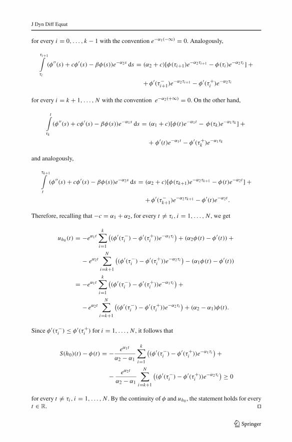
J Dyn Diff Equat

for every i = 0, . . . , k − 1 with the convention e−α1(−∞) = 0. Analogously,

τi+1∫

τi

(φ′′(s)+ cφ′(s)− βφ(s))e−α2s ds = (α2 + c)[φ(τi+1)e−α2τi+1 − φ(τi )e

−α2τi ] +

+φ′(τ−i+1)e

−α2τi+1 − φ′(τ+i )e

−α2τi

for every i = k + 1, . . . , N with the convention e−α2(+∞) = 0. On the other hand,

t∫

τk

(φ′′(s)+ cφ′(s)− βφ(s))e−α1s ds = (α1 + c)[φ(t)e−α1t − φ(τk)e−α1τk ] +

+ φ′(t)e−α1t − φ′(τ+k )e

−α1τk

and analogously,

τk+1∫

t

(φ′′(s)+ cφ′(s)− βφ(s))e−α2s ds = (α2 + c)[φ(τk+1)e−α2τk+1 − φ(t)e−α2t ] +

+φ′(τ−k+1)e

−α2τk+1 − φ′(t)e−α2t .

Therefore, recalling that −c = α1 + α2, for every t �= τi , i = 1, . . . , N , we get

uh0(t) = −eα1tk∑

i=1

((φ′(τ−

i )− φ′(τ+i ))e

−α1τi)+ (α2φ(t)− φ′(t))+

− eα2tN∑

i=k+1

((φ′(τ−

i )− φ′(τ+i ))e

−α2τi)− (α1φ(t)− φ′(t))

= −eα1tk∑

i=1

((φ′(τ−

i )− φ′(τ+i ))e

−α1τi)+

− eα2tN∑

i=k+1

((φ′(τ−

i )− φ′(τ+i ))e

−α2τi)+ (α2 − α1)φ(t).

Since φ′(τ−i ) ≤ φ′(τ+

i ) for i = 1, . . . , N , it follows that

S(h0)(t)− φ(t) = − eα1t

α2 − α1

k∑

i=1

((φ′(τ−

i )− φ′(τ+i ))e

−α1τi)+

− eα2t

α2 − α1

N∑

i=k+1

((φ′(τ−

i )− φ′(τ+i ))e

−α2τi) ≥ 0

for every t �= τi , i = 1, . . . , N . By the continuity of φ and uh0 , the statement holds for everyt ∈ R. �

123

J Dyn Diff Equat

3 An Existence Result

Consider the following functional equation:

u′′(t)+ cu′(t)+ F(u)(t) = 0, t ∈ R (3.1)

where c > 0, and F : C(R) → C(R) is a given operator.In the sequel we assume that there exists β > 0 such that the following conditions hold:

(H1) 0 ≤ u(t) ≤ 1 for every t ∈ R ⇒ 0 ≤ F(u)(t)+ βu(t) ≤ β for every t ∈ R.

(H2) u monotone decreasing ⇒ F(u)+ βu monotone decreasing.

Fixed a value β > 0 in such a way that conditions (H1) and (H2) hold, define F : C(R) →C(R) by

F(u)(t) = −F(u)(t)− βu(t), t ∈ R.

By using the operator F , Eq. (3.1) can be equivalently written as follows:

u′′(t)+ cu′(t)− βu(t) = F(u)(t), t ∈ R. (3.2)

Setting M := 2β√c2+4β

, let us consider the following subset of BC(R):

:= {u ∈ C(R) : 0 ≤ u(t) ≤ 1 for all t ∈ R, u is decreasing, |u(t1)− u(t2)| ≤ M |t1 − t2|for all t1, t2 ∈ R}.

By assumption (H1), we have F(u) ∈ BC(R) for every u ∈ , so we can define thecomposition operator

G(u) := S(F(u)), for u ∈ .Notice that a function u ∈ is a fixed point for the operator G if and only if it is a solution

of Eq. (3.2). Hence the study of the existence of solutions of (3.1) reduces to the existenceof fixed points for the operator G, as we do in the following theorem.

Theorem 3.1 Assume that conditions (H1) and (H2) are satisfied. Moreover, assume thatthe operator F : BCρ(R) → BCρ(R) is continuous for some 0 < ρ < min{−α1, α2}. Then,Eq. (3.1) has a solution in .

Proof First note that as an immediate consequence of conditions (H1), (H2) and statements(iii)–(iv) of Lemma 2.1, we have

G() ⊆ .

Moreover, G is continuous in with respect to the norm ‖ · ‖ρ , indeed if (un)n is a sequencein converging to u ∈ , then

‖G(un)− G(u)‖ρ = ‖S(F(un)− S(F(u))‖ρ ≤ k ‖F(un)− F(u)‖ρ≤ k‖F(un)− F(u)‖ρ + kβ‖un − u‖ρ

where k = k(ρ) is the constant given by Lemma 2.2. Then, the continuity of G follows fromthe continuity of F .

Observe now that is a nonempty, convex subset of the Banach space BCρ(R), so inorder to apply the Schauder fixed point theorem it remains to show that is compact.

123

J Dyn Diff Equat

To this purpose, let (un)n be a given sequence in . By the definition of we get that(un)n is equibounded and equiuniformly continuous. So, by the Ascoli-Arzelà theorem, itsrestriction to the interval I1 = [−1, 1] admits a subsequence (un1,k )k uniformly convergentin I1 to a function v1(t). Similarly, in the interval I2 = [−2, 2] the sequence (un1,k )k admitsa further subsequence (un2,k )k uniformly convergent in I2 to a function v2(t). Of course,v2(t) = v1(t) for t ∈ I1. By induction, for every m ∈ N the sequence (unm−1,k )k admitsa further subsequence (unm,k )k uniformly convergent in Im to a function vm(t) satisfyingvm(t) = vm−1(t) for t ∈ Im−1.

Consider now the “diagonal” subsequence (unk,k )k and the function v : R → R definedby v(t) = vm(t) if t ∈ Im . Clearly, v is well defined, continuous and decreasing; moreover0 ≤ v(t) ≤ 1 for any t ∈ R, and |v(t1)− v(t2)| ≤ M |t1 − t2| for and any t1, t2 ∈ R; that is,v belongs to .

Finally, fix ε > 0 and choose L ∈ N such that e−ρ|t | < ε2 for any t with |t | > L . We have

|unk,k (t)− v(t)|e−ρ|t | ≤ 2e−ρ|t | < ε, (3.3)

for any t with |t | > L . On the other hand, since {unL ,k (t)} converges to vL(t) = v(t)uniformly on IL , and since {unk,k } is a subsequence of {unL ,k (t)}, we have

supt∈[−L ,L]

|unk,k (t)− v(t)| → 0, k → ∞.

Hence, there exists k > L such that for any k > k one has

|unk,k (t)− v(t)|e−ρ|t | ≤ |unk,k (t)− v(t)| < ε for every t ∈ [−L , L].Consequently, taking (3.3) into account we get

||unk,k − v||ρ < ε for every k > k

i.e. the sub-sequence (unk,k )k converges to v with respect to the norm ‖ · ‖ρ and then iscompact.

By applying the Schauder fixed point Theorem we achieve the existence of a fixed pointfor the operator G and this concludes the proof. �

The following Proposition concerning the asymptotical properties of the decreasing solu-tions of Eq. (3.1), will be used in the sequel.

Proposition 3.2 Assume that conditions (H1) and (H2) are satisfied. Moreover, assume thatthe operator F : BCρ(R) → BCρ(R) is continuous for some 0 < ρ < min{−α1, α2} andhas constant sign, i.e.

F(u)(t) ≤ 0 (or F(u)(t) ≥ 0) for every decreasing, non-negative u ∈ C(R),

and every t ∈ R. (3.4)

Then, if u ∈ C2(R) is a decreasing solution of Eq. (3.1), with 0 ≤ u(t) ≤ 1, it satisfies

u′(±∞) = u′′(±∞) = 0,

and the constant c has the same sign as the operator F.

Proof Fix τ < t . Integrating the Eq. (3.1) in (τ, t) we obtain

u′(t) = u′(τ )− c(u(t)− u(τ ))−t∫

τ

F(u)(s) ds

123

J Dyn Diff Equat

and by the assumption (3.4) we deduce the existence in R∪{±∞} of the limit limt→+∞u′(t),which has to be null by the boundedness of the function u(t). Similarly we can prove thatu′(−∞) = 0. Moreover, from the previous equation, taking the limits as t → +∞, τ → −∞one derives that c has the sign of the operator F .

Finally, by assumptions (H1)-(H2) we have that F(u)(t)+βu(t) is a decreasing boundedfunction, so there exist in R the limits F(u)(±∞). Hence, by Eq. (3.1) there exist inR also the limits u′′(±∞), which have to be null owing to the boundedness of u′ as|t | → +∞. �

4 Boundary Value Problem

In this section, we finally investigate the solvability of the following boundary value problem:{

u′′(t)+ cu′(t)+ F(u)(t) = 0, a.e. t ∈ R

u(−∞) = 1, u(+∞) = 0.(4.1)

Note that the solution of Eq. (3.1) found in the proof of Theorem 3.1 may be trivial,i.e. constant. In order to obtain heteroclinic solutions we need further conditions, such as theexistence of suitable super and sub-solutions. To this end, let us now introduce the followingdefinition.

Definition 4.1 A decreasing function φ ∈ BC(R) is said to be a super-solution [respectivelysub-solution] of (3.1) if there exist at most finitely many points, denoted by −∞ = τ0 <

τ1 < · · · < τN < τN+1 = +∞, such that:

(i) φ ∈ C2(τi , τi+1), with φ′, φ′′ bounded, for every i = 0, . . . , N ;(ii) the limits φ′(τ−

i ), φ′(τ+

i ) exist and satisfy φ′(τ−i ) ≥ φ′(τ+

i ) [φ′(τ−i ) ≤ φ′(τ+

i )],i = 1, · · · , N ;

(iii) the following differential inequality holds:

φ′′(t)+ cφ′(t)+ F(φ)(t) ≤ 0 [φ′′(t)+ cφ′(t)+ F(φ)(t) ≥ 0]for every t �= τi , i = 1, . . . , N .

Remark 4.2 The enlargement of the class of admissible super and sub-solutions to possiblenon-smooth functions is motivated by the difficulty to find well-ordered smooth super andsub-solutions, due to the lack of monotonicity of F (see [13] for recent comparison resultsfor non-functional equations). In this setting, the relation between the left and right deriv-atives in the non-smoothness points (condition (ii)) is fundamental. Recently, some papersappeared using a more general definition, without requiring (ii) (see [7,8,12,15,17]), but thearguments there used do not work (see [18]).

The following theorem provides sufficient conditions for the solvability of problem (4.1).

Theorem 4.3 Assume that there exists β > 0 such that conditions (H1) and (H2) are satis-fied. Moreover, assume that the following condition holds:

(H3) u1(t) ≤ u2(t) for every t ∈ R ⇒ F(u1)(t) + βu1(t) ≤ F(u2)(t) + βu2(t) forevery t ∈ R.

For fixed 0 < ρ < min{−α1, α2}, assume that the operator F : C(R) → C(R) is continu-ous with respect to the norm ‖ · ‖ρ . Finally, assume that there exist a pair φ, ψ of sub and

123

J Dyn Diff Equat

super-solutions of (3.1) such that 0 ≤ φ(t) ≤ ψ(t) ≤ 1 for every t ∈ R. Then, Eq. (3.1)admits a decreasing solution u ∈ , such that

φ(t) ≤ u(t) ≤ ψ(t) for every t ∈ R.

If φ and ψ further satisfy

φ(−∞) = 1, ψ(+∞) = 0,

then u solves the boundary value problem (4.1) too.

Proof Let and G be as in Sect. 3. Consider the following subset of BC(R):

= {u ∈ : φ(t) ≤ u(t) ≤ ψ(t)}.Of course, is also nonempty and convex. Moreover, since it is a closed subset of, whichis compact, is also compact in the Banach space BCρ(R).

Observe now that G() ⊆ . Indeed, we already proved that G() ⊆ , so it suffices toshow that

φ(t) ≤ G(u)(t) ≤ ψ(t) for every u ∈ , t ∈ R. (4.2)

Let us prove that G(u)(t) ≥ φ(t) for every t ∈ R (the other inequality being similar). Noticethat condition (H3) implies that F(u)(t) ≤ F(φ)(t) for every t ∈ R. So, defined η : R → R

by η(t) = φ′′(t) + cφ′(t) − βφ(t), a.e. t ∈ R, we have η ∈ L∞(R), and F(φ)(t) ≤ η(t)a.e. t ∈ R as φ is a sub-solution. Moreover, S(η)(t) ≥ φ(t) for every t ∈ R by Lemma 2.4.Consequently, by the monotonicity the of operator S we get

G(u)(t) = S(F(u))(t) ≥ S(F(φ))(t) ≥ S(η)(t) ≥ φ(t) for every t ∈ R.

Thus, G() ⊆ . Moreover, we already proved in Theorem 3.1 that G is continuous in .So, by applying again the Schauder fixed point theorem it follows that G has a fixed pointu ∈ , which results to be a solution of Eq. (3.1).

Moreover, if 0 ≤ φ(t) ≤ u(t) ≤ ψ(t) ≤ 1 for every t ∈ R, the conditions φ(−∞) = 1and ψ(+∞) = 0 respectively imply that u(−∞) = 1 and u(+∞) = 0 and, consequently, uis a solution of problem (4.1). �

Concerning the properties of the set of the values of the speed c for which problem (4.1)admits solutions, we are able to prove that it is closed provided that the problem is autono-mous, in the sense specified by the following definition.

Definition 4.4 We will say that the boundary value problem (4.1) is autonomous, if thefollowing property holds:

u(t) is a solution to (4.1) ⇒ u(t + k) is a solution to (4.1) too, for every k ∈ R.

Proposition 4.5 Let F : C(R) → C(R) be a continuous operator with respect to the norm‖ ·‖ρ , satisfying assumptions (H1)-(H2) and (3.4). Assume that problem (4.1) is autonomousand

There exist limt→±∞ F(u)(t) �= 0 for every decreasing function u ∈ C(R)

such that u(±∞) ∈ (0, 1). (4.3)

Let C denote the set of the admissible speeds for problem (4.1), i.e.

C := {c > 0 : problem (4.1) admits a decreasing solution}.Then C is a closed set (possibly empty).

123

J Dyn Diff Equat

Proof As we already observed in the previous section, a decreasing function u is a solutionto Eq. (3.1) if and only if it is a fixed point for the operator G. Since now the parameter cis not fixed, from now on we use the notation Gc to make explicit the dependence on thespeed c.

Assume that C is nonempty and take a sequence (cn)n in C converging to a value c∗.Let un(t) denote a decreasing solution to problem (4.1) for c = cn , satisfying un(0) = 1

2(this is possible since the problem is autonomous). By Lemma 2.1, part (iii), we deduce that|u′

n(t)| ≤ 2β√c2

n+4β≤ √

β for every t ∈ R. Hence, by the same argument used in the proof of

Theorem 3.1 for proving that is compact, one can show that there exists a sub-sequence,again denoted (un)n , uniformly converging in every compact set to a decreasing function u∗.

By the continuity of operator F and assumption (H1), we get that (F(un))n is an equi-bounded sequence pointwise convergent to F(u∗). So, by Proposition 2.3 we deduce

Gc∗(u∗)(t) = limn→+∞Gcn (un)(t) = lim

n→+∞un(t) = u∗(t).

Therefore, the function u∗ is a fixed point for the operator Gc∗ and this means that it is asolution of Eq. (3.1) for c = c∗. Moreover, u∗(0) = 1

2 , so u∗ is not one of the trivial solutionsu(t) ≡ 0 or u(t) ≡ 1.

Let us denote by �− := u∗(−∞) ≥ 12 and �+ := u∗(+∞) ≤ 1

2 . Since by Proposition 3.2we have (u∗)′(−∞) = (u∗)′′(−∞) = 0, then by assumption (4.3) we deduce �− = 1 and�+ = 0. Hence u∗ is a solution to problem (4.1) for c = c∗. �Remark 4.6 Notice that in the previous Proposition we have just proved that C is closed, butactually we neither know if it is connected (an interval) nor if it is bounded or unbounded(see Sect. 6 for a more detailed discussion on this subject).

5 Applications and Examples

In this section, we present some non-local reaction-diffusion equations which can be handledby means of the approach we introduced here. More in detail, as mentioned in the Introduc-tion, we refer to models whose reaction term has a retarded component or depends on aconvolution integral.

5.1 Reaction-Diffusion Equations with Delay

For fixed T ∗ > 0, let f : C([−T ∗, 0]) → [0,+∞) be a given continuous operator (withrespect to the usual topology in C([−T ∗, 0])). Let us consider the following partial differ-ential equation

∂v

∂τ= ∂2v

∂x2 + f (vτ (x)) (5.1)

where vτ (x) ∈ C([−T ∗, 0]) is the function defined by vτ (x)(θ) := v(τ + θ, x), for θ ∈[−T ∗, 0].

In the sequel we will assume that the constant functions 0 and 1 are stationary states forthe Eq. (5.1), that is

f (1) = f (0) = 0

(here and later on, k denotes the constant function w(θ) ≡ k, θ ∈ [−T ∗, 0]).

123

J Dyn Diff Equat

When searching for traveling wave solutions connecting the equilibria 0 and 1, put t :=x − cτ, u(t) = u(x − cτ) and consider the functional boundary value problem

{u′′(t)+ cu′(t)+ f (ut,c) = 0u(−∞) = 1, u(+∞) = 0

(5.2)

where ut,c ∈ C([−T ∗, 0]) is the function defined by

ut,c(θ) := u(t − cθ).

In order to treat such a problem by means of the approach presented here, we deal withreaction terms having the following structure:

f (w) = f1(w) · f2(w(0))

where f1 : C([−T ∗, 0]) → [0,+∞), f2 : R → [0,+∞) are continuous and satisfy thefollowing conditions.

(F1-A): f1(0) = 0, f1(k) > 0 for every k > 0;(F1-B): f1 is increasing, that is f1(u) ≤ f1(v) whenever u(θ) ≤ v(θ) for every

θ ∈ [−T ∗, 0];(F2-A): f2(1) = 0, f2(s) > 0 for every s ∈ [0, 1);(F2-B): f2 is Lipschitzian with Lipschitz constant L .

For every c > 0 let Fc : C(R) → C(R) denote the operator defined by

Fc(u)(t) := f (ut,c) = f1(u(t − cθ)) f2(u(t)).

Of course, the operator Fc is continuous (with respect to the norm ‖ · ‖ρ).The following Lemma concerns the applicability of the method presented in the previous

sections.

Lemma 5.1 Assume that the operator f satisfies the properties listed above. Then for everyc > 0 the operator Fc satisfies assumptions (H1)-(H3) with the constant β := L f1(1) > 0.

Proof As for property (H1), since f (w) ≥ 0 for everyw ∈ C([−T ∗, 0]), of course Fc(u)(t)+βu(t) ≥ 0 for every u ∈ C(R). Moreover, by (F2-A) and (F2-B) we have f2(s) ≤ L(1 − s)for every s ∈ [0, 1], so being f1(ut,c) ≤ f1(1) by (F1-B), we deduce f1(ut,c) f2(u(t)) ≤β(1 − u(t)), that is Fc(u)(t)+ βu(t) ≤ β.

If u is monotone decreasing, then for fixed t1 < t2 we have u(t1 − cθ) ≥ u(t2 − cθ)for every θ ∈ [−T ∗, 0], that is ut1,c(θ) ≥ ut2,c(θ) for every θ ∈ [−T ∗, 0]. Hence, byassumption (F1-B) we get f1(ut1,c) ≥ f1(ut2,c). Moreover, by (F2-B) we have f2(u(t1)) ≥f2(u(t2))− L[u(t1)− u(t2)], so

f1(ut1,c) f2(u(t1)) ≥ f1(ut2,c) f2(u(t2))− L f1(ut2,c)[u(t1)− u(t2)]≥ f1(ut2,c) f2(u(t2))− β[u(t1)− u(t2)].

Hence,

f1(ut1,c) f2(u(t1))+ βu(t1) ≥ f1(ut2,c) f2(u(t2))+ βu(t2)

i.e. condition (H2).Finally, if u, v ∈ C(R) satisfy u(t) ≤ v(t) for every t ∈ R then f1(ut,c) ≤ f1(vt,c) and

f2(v(t)) ≥ f2(u(t))− L[v(t)− u(t)], so

f1(vt,c) f2(v(t)) ≥ f1(ut,c) f2(u(t))− L f1(ut,c)[v(t)− u(t)]≥ f1(ut,c) f2(u(t))− β[v(t)− u(t)],

123

J Dyn Diff Equat

that is f (vt,c)+ βv(t) ≥ f (ut,c)+ βu(t), i.e. condition (H3). �

The following existence result shows that a pair of ordered super- and sub-solutions canbe found under very mild assumptions on the non-functional term f2, provided that the func-tional term f1 depends on a simple discrete delay. Moreover, we also obtain an estimate ofthe rate of decay as t → +∞. In this context, we adopt the notation

u(t) ≈ e−λt ⇔ u(t)eλt → � ∈ (0,+∞) as t → +∞. (5.3)

Theorem 5.2 Let

f1(wt,c) := w(t + cT ) for some T ∈ [0, T ∗],and let f2 satisfy conditions (F2-A), (F2-B), and

f2(s) ≤ f2(0)(1 − s) for every s ∈ [0, 1]. (5.4)

Then, for every c > 2√

f2(0) there exists a positive value T0 = T0(c) such that if 0 ≤ T ≤ T0

the boundary value problem (5.2) with f (w) = f1(w)· f2(w(0)) admits a decreasing solutionu. Moreover, u(t) ≈ e−λt as t → +∞, for some λ ≤ 1

2 (c −√c2 − 4 f2(0)).

Proof In view of Lemma 5.1 and Theorem 4.3, we only need to find a pair of ordered superand sub-solutions. To this aim, put K := f2(0) and let us consider the function

H(�, c, T ) := �2 − c�+ K e−c�T , for �, T ≥ 0; c > 2√

K . (5.5)

Since H is a continuous function satisfying H(0, c, T ) = K > 0 and H( c2 , c, T ) = c2

4 −c2

2 + K e− c22 T ≤ K − c2

4 < 0, the set

Ac,T :={� ∈

(0,

c

2

): H(�, c, T ) = 0

}

is a nonempty closed set. Put

λ = λ(c, T ) := max Ac,T . (5.6)

As a consequence of the previous definition, for every c, T there exists a positive valueε = ε(c, T ) < λ, such that

H(λ+ ε, c, T ) = (λ+ ε)2 − c(λ+ ε)+ K e−c(λ+ε)T < 0. (5.7)

Now, given M > 1, consider the function

φ(t) := max{0, (1 − Me−εt )e−λt }.Let t∗ denote the positive value such that Me−εt∗ = 1. Observe that 0 = φ′(t∗−) <

φ′(t∗+), moreover if t < t∗ then φ′(t) = φ′′(t) = 0, so φ′′(t) + cφ′(t) + f (φt,c) ≥ 0.Instead, if t > t∗ (and t + cT > t∗ too) then

φ′(t) = −λe−λt + M(ε + λ)e−(ε+λ)t ; φ′′(t) = λ2e−λt − M(ε + λ)2e−(ε+λ)t .

If L denotes the Lipschitz constant for f2, put h := LK we have

f2(s) ≥ K (1 − hs) for every s ∈ [0, 1]. (5.8)

123

J Dyn Diff Equat

Then,

φ′′(t)+ cφ′(t)+ f (φt,c) ≥ φ′′(t)+ cφ′(t)+ Kφ(t + cT )[1 − hφ(t)]= e−λt {λ2 − M(ε + λ)2e−εt − cλ+ cM(ε + λ)e−εt +

+ K (1 − Me−εt e−εcT )e−cλT [1 − h(1 − Me−εt )e−λt ]}≥ e−λt {(λ2 − cλ+ K e−cλT )− Me−εt [(ε + λ)2 − c(ε + λ) +

+ K e−c(ε+λ)T ] − K he−λt e−λcT }= e−λt {H(λ, c, T )− Me−εt H(λ+ ε, c, T )− K he−λ(t+cT )}≥ Me−(λ+ε)t

{−H(λ+ ε, c, T )− L

Me−λcT

},

since H(λ, c, T ) = 0 and (λ− ε)t > 0. By (5.7) we deduce that there exists a positive valueM0 such that if M ≥ M0 the last term in the previous chain of inequalities is positive, andthis implies that φ is a sub-solution for every M ≥ M0.

In order to find a super-solution, consider the function

ψ(t) := 1

1 + αeλtwith α > 0 and λ = λ(c, T ) defined in (5.6).

Of course, ψ is a decreasing function satisfying ψ(−∞) = 1, ψ(+∞) = 0.Observe that

ψ ′(t) = −αλ eλt

(1 + αeλt )2, ψ ′′(t) = αλ2eλt

(1 + αeλt )3(αeλt − 1).

Therefore, by (5.4) we have

ψ ′′(t)+ cψ ′(t)+ f (ψt,c) ≤ ψ ′′(t)+ cψ ′(t)+ Kψ(t + cT )[1 − ψ(t)]= αλ2eλt (αeλt − 1)

(1 + αeλt )3− αλceλt

(1 + αeλt )2+ K

αeλt

(1 + αeλt )(1 + αeλt ecλT )

= αeλt

(1 + αeλt )3(1 + αeλt ecλT )

{λ2(αeλt − 1)(1 + αeλt ecλT )− λc(1 + αeλt ) ·

·(

1 + αeλt ecλT)

+ K (1 + αeλt )2}.

Hence, putting A(t) := αeλt

(1+αeλt )3(1+αeλt ecλT )> 0 and recalling that λ2 − cλ+ K e−cλT = 0,

the last term in the previous chain of equalities becomes

A(t){α2e2λt ecλT (λ2 − cλ+ K e−cλT )+αeλt [λ2 − cλ+ ecλT (−λ2 − cλ+ 2K e−cλT )]+

+ (K−cλ−λ2)} = A(t)

{−αeλt [K e−cλT +ecλT (2λc−3K e−cλT )]−(2cλ−K−K e−cλT )

}.

(5.9)

Let us now consider the function h(c) := cλ(c, 0) = c2 (c − √

c2 − 4K ), for c > 2√

K .Observe that h(c) is a strictly decreasing function, indeed

h′(c) = 1

2

(c −

√c2 − 4K

)+ c

2

(1 − c√

c2 − 4K

)= 1

2

[2c − c2

√c2 − 4K

−√

c2 − 4K

]

= c√

c2 − 4K − c2 + 2K√c2 − 4K

< 0.

123

J Dyn Diff Equat

Then,

c · λ(c, 0) = h(c) > K = limc→+∞ h(c), for every c > 2

√K . (5.10)

So, put

γ (c, T ) := K e−cλT + ecλT (2λc − 3K e−cλT ), δ(c, T ) := 2cλ− K − K e−cλT ,

by (5.10) we have γ (c, 0) = δ(c, 0) = 2(h(c)− K ) > 0. Hence, for every c > 2√

K thereexists a positive value T0 = T0(c) such that γ (c, T ), δ(c, T ) > 0 if T ∈ [0, T0]. Therefore,for such values of T we get that the term in (5.9) is negative for every t ∈ R and this meansthat ψ is a super-solution.

Let us now show that if we take α < 1 − 1M , then φ(t) < ψ(t) for every t ∈ R. Such a

relation is trivial for t ≤ t∗, whereas for every t ≥ t∗, since e−λt < e−εt ≤ e−εt∗ = 1M , we

have

(1 − Me−εt )(e−λt + α) ≤ e−λt + α ≤ 1

M+ α < 1,

hence φ(t) = (1 − Me−εt )e−λt < 11+αeλt = ψ(t) for every t ≥ t∗.

Therefore, by applying Theorem 4.3, we deduce that the differential equation in (5.2)admits a decreasing solution u satisfying φ(t) ≤ u(t) ≤ ψ(t) for every t ∈ R. This imme-diately implies that u(+∞) = 0, so it remains to show that u(−∞) = 1.

In order to do this, observe that by Proposition 3.2 we have u′(−∞) = u′′(−∞) = 0, soalso limn→+∞ f (u−n,c) = 0. Put � := u(−∞), it is easy to see that the sequence of function(u−n,c(θ))n uniformly converges to the constant function u(θ) ≡ �. Indeed, for every fixedε > 0, let tε be such that |u(t)− �| < ε for every t < tε . So, if we take n = nε > cT ∗ − tεthen for every n ≥ nε and θ ∈ [−T ∗, 0] we have −n − cθ ≤ −nε + cT ∗ < tε , so

|u−n,c(θ)− �| = |u(−n − cθ)− �| < ε for every θ ∈ [−T ∗, 0], n ≥ nε .

Thus, by the continuity of f we get f (�) = 0 and being � > 0, by assumptions (F1-A) and(F2-A) we deduce � = 1.

Finally, as regards the rate of decay, since φ(t), ψ(t) ≈ e−λt as t → +∞, also u(t) does.Moreover, since H(λ(c, 0), c, T ) < 0, we have λ ≤ λ(c, 0) = 1

2 (c − √c2 − 4K ). �

In the previous theorem, we fixed a generic speed c > 2√

K and show that if the delayT is sufficiently small there exists a front having speed c. In the following result we changepoint of view, indeed we show that for every fixed delay T > 0 there exists a bounded intervalsuch that if the speed c belongs to it then there exists a traveling wave having speed c.

Theorem 5.3 Under the same assumption of Theorem 5.2, for every 0 < T < 1f2(0)

log 43

there exists a value c∗ = c∗(T ) > 2√

f2(0) such that for every c ∈ [2√f2(0), c∗] the

boundary value problem (5.2) with f (w) = f1(w) · f2(w(0)) admits a decreasing solutionu. Moreover, u(t) ≈ e−λt as t → +∞ (see (5.3), where λ ≤ 1

2 (c − √c2 − 4 f2(0)), andc∗(T ) → +∞ as T → 0.

Proof Put, as above, K := f2(0), and considered the function H(�, c, t) defined in (5.5),

observe that H(√

K2 , 2

√K , T ) = K

4 −K +K e−K T = K (e−K T − 34 ) > 0, due to the assump-

tion on the upper limitation of T . Then, λ(2√

K , T ) >√

K2 , i.e. 2

√K · λ(2√

K , T ) > K .Therefore, there exists a value c∗ = c∗(T ) > 2

√K such that

c · λ(c, T ) > K for every c ∈ (2√K , c∗). (5.11)

123

J Dyn Diff Equat

The proof of the present result proceeds as that of Theorem 5.2 until formula (5.9). Fromthere on, observe that by (5.11) we get

K e−cλT + ecλT (2cλ− 3K e−cλT ) > K e−cλT + 2K ecλT − 3K

= K e−cλT (1 + 2e2cλT − 3ecλT ) > 0

and 2cλ − K e−cλT − K > K (1 − e−cλT ) > 0, implying again that ψ is a super-solution.Hence, from now on the proof proceeds as that of the previous theorem.

The assertion for c = 2√

K and c = c∗ is a consequence of the closure of the range ofthe admissible speeds proved in Proposition 4.5.

Finally, as regards the behavior of c∗ for T small, observe that

c∗∗(T ) := sup{c : c λ(c, T ) > K }is a continuous function of T taking value on R ∪ {+∞} and c∗∗(0) = +∞, by virtue of(5.10). So, the assertion follows. �

We present now an example of applications of the results in this section.

Example 5.4 Let us consider the delayed reaction-diffusion equation

vτ (τ, x) = vxx (τ, x)+ Kv(τ − T, x) (1 − v(τ, x))p , with p ≥ 1.

Put

f (w) := Kw(−T ) (1 − w(0))p , for w ∈ C([−T, 0],we can apply Theorems 5.2 and 5.3 to deduce the existence of travelling fronts.

5.2 Non-Functional Fisher–KPP Equations

Despite the present research is motivated by the study of non-local reaction-diffusion equa-tions, we wish to show how we can fruitfully treat also the non-functional case by means ofour approach.

Let us consider the classical equation

u′′ + cu′ + f (u) = 0 (5.12)

where f : [0, 1] → R is a Lipschitzian Fisher-type term, that is satisfying f (u) > 0 in(0, 1), f (0) = f (1) = 0. We define F : C(R) → C(R) by

F(u)(t) ={

f (u(t)) if u(t) ∈ [0, 1]0 otherwise.

Notice that F is a continuous operator with respect the norm ‖ · ‖ρ , for every ρ > 0, sincef is a continuous function.

Set β := supu �=v∣∣∣ f (u)− f (v)

u−v∣∣∣ the Lipschitz constant of f , it is immediate to verify that

the operator F satisfies the assumptions (H1) − (H3). Moreover, as an application ofTheorem 4.3, we can derive the following result, which is well-known.

Proposition 5.5 Let f be a function as above, differentiable in a right neighborhood of 0with f ′(0) > 0, such that there exist f ′′(0) > −∞ and

0 < f (u) ≤ f ′(0)u for every u ∈ (0, 1). (5.13)

123

J Dyn Diff Equat

Then, for every c ≥ 2√

f ′(0) there exists a decreasing solution u of the problem{

u′′ + cu′ + f (u) = 0u(−∞) = 1, u(+∞) = 0.

Moreover, u(t) ≈ e−λt as t → +∞ (see (5.3)), where λ = 12 (c −√c2 − 4 f ′(0)).

Proof Since f ′′(0) > −∞, then there exists positive values ν, δ > 0 such that f ′(u) ≥f ′(0)− νu for every u ∈ [0, δ), with f ′(0) > 0 owing to assumption (5.13). So, integrating,we deduce

f (u) ≥ f ′(0)u − ν

2u2 = f ′(0)u

(1 − ν

2 f ′(0)u

)for every u ∈ [0, δ).

Therefore, considered the function φ(t) := δmax{0, (1 − Me−εt )e−λt } ≤ δ (with λ =12 (c −√c2 − 4 f ′(0))), by means of the same proof of Theorem 5.2 (rewritten for T = 0),one deduce that the function φ is a sub-solution.

Moreover, let us consider now the function ψ(t) := min{1, e−λt }. Observe that 0 =ψ ′(0−) > ψ ′(0+) and since f (1) = 0, it is immediate to verify that ψ ′′(t) + cψ ′(t) +f (ψ(t)) = 0 for every t < 0. Instead, if t > 0 then

ψ ′′(t)+ cψ ′(t)+ f (ψ(t)) ≤ ψ ′′(t)+ cψ ′(t)+ f ′(0)ψ(t) = e−λt (λ2 − cλ+ f ′(0)) = 0.

Therefore, ψ is a super-solution. Finally, one can easily verify that φ(t) < ψ(t) for everyt ∈ R. Hence, by applying Theorem 4.3 we deduce the existence of a decreasing solutionu(t) satisfying φ(t) ≤ u(t) ≤ ψ(t) for every t ∈ R, implying u(+∞) = 0 with u ≈ e−λt ast → +∞. Being f (u) > 0 for every u ∈ (0, 1) and applying Proposition 3.2, we necessarilyhave u(−∞) = 1 and this concludes the proof. �5.3 Reaction-Diffusion Equations With Convolution Integrals

Let us consider the non-local reaction-diffusion equation

vτ (τ, x) = vxx (τ, x)+ f0(v(τ, x))

+∞∫

−∞�(x − σ)v(τ, σ ) dσ,

where � : R → R is a continuous, non-negative map satisfying

+∞∫

−∞�(s) ds = 1,

and f0 : R → [0,+∞) is a continuous function satisfying the following conditions:

(F0-A): f0(1) = 0, f0(s) > 0 for every s ∈ [0, 1);(F0-B): f0 is Lipschitzian with Lipschitz constant L .

When searching for traveling wave solutions v(τ, x) = u(x − cτ), the change of vari-able t = x − cτ leads to consider the functional boundary value problem (recall that theconvolution product is commutative)

{u′′(t)+ cu′(t)+

( ∫ +∞−∞ �(s)u(t − s) ds

)f0(u(t)) = 0

u(−∞) = 1, u(+∞) = 0.(5.14)

123

J Dyn Diff Equat

In order to treat such a problem by means of the approach presented here, define F : C(R) →C(R) by

F(u)(t) =⎛

⎝+∞∫

−∞�(s)u(t − s) ds

⎞

⎠ f0(u(t)), t ∈ R.

Notice that F is a continuous operator.The following Lemma concerns the applicability of the method presented in the previous

sections.

Lemma 5.6 Assume that the function f0 satisfies the properties listed above. Then, the oper-ator F satisfies assumptions (H1)-(H3) with β ≥ L.

Proof As for property (H1), assume 0 ≤ u(t) ≤ 1 for any t ∈ R. Then, F(u)(t)+βu(t) ≥ 0for any t . Moreover, by (F0-A) and (F0-B) we have f0(s) ≤ L(1− s) for every s ∈ [0, 1], so

⎛

⎝+∞∫

−∞�(s)u(t − s) ds

⎞

⎠ f0(u(t)) ≤ L(1 − u(t)),

and, being β ≥ L , we deduce

−F(u)(t)− βu(t)+ β ≥ (β − L)(1 − u(t)) ≥ 0

for any t . Hence, condition (H1) holds.Assume now that u ∈ C(R) is monotone decreasing and let us show that F(u) + βu is

monotone decreasing too. Fixed t1 < t2 we have u(t1) ≥ u(t2), so

+∞∫

−∞�(s)u(t1 − s) ds ≥

+∞∫

−∞�(s)u(t2 − s) ds,

and by (F0-B) we have f0(u(t1)) ≥ f0(u(t2))− L(u(t1)− u(t2)). Therefore,

F(u)(t2)−F(u)(t1) =⎛

⎝+∞∫

−∞�(s)u(t2−s) ds

⎞

⎠ f0(u(t2))−⎛

⎝+∞∫

−∞�(s)u(t1−s) ds

⎞

⎠ f0(u(t1))

≤⎛

⎝+∞∫

−∞�(s)u(t2 − s) ds

⎞

⎠ [ f0(u(t2))− f0(u(t1))]

≤ L

⎛

⎝+∞∫

−∞�(s)u(t2 − s) ds

⎞

⎠ [u(t1)− u(t2)] ≤ β[u(t1)− u(t2)]

since β ≥ L . Hence, condition (H2) is satisfied. The proof of the validity of (H3) isanalogous. �

In order to present a concrete application of our existence result, let us consider the par-ticular function

�0(t) = b

2e−b|t |, t ∈ R, for some b > 0. (5.15)

123

J Dyn Diff Equat

The following result states that imposing some further conditions on the function f0 and theconstants b, c, a pair of ordered super and sub-solutions can be found and consequently theboundary value problem (5.14) admits solutions.

Theorem 5.7 Let �0 be defined by (5.15) and let f0 satisfy conditions (F0-A) - (F0-B).Assume that b > 2

√f0(0) and

f0(s) ≤ f0(0)(1 − s) for every s ∈ [0, 1]. (5.16)

Then, for every c ∈ [c∗1, c∗

2], where

c∗1 :=

√

2

(b2 − b

√b2 − 4 f0(0)

), c∗

2 :=√

2

(b2 + b

√b2 − 4 f0(0)

), (5.17)

the boundary value problem (5.14) admits a decreasing solution u. Moreover, u(t) ≈ e−λt

as t → +∞ (see (5.3)), for a suitable λ < c/2.

Proof In view of Lemma 5.6 and Theorem 4.3, we only need to find a pair of ordered superand sub-solutions.

First of all, observe that it suffices to prove the assertion for c ∈ (c∗1, c∗

2). Indeed, in thepresent framework all the assumptions of Proposition 4.5 are satisfied and then the range ofthe values of c for which the boundary value problem (5.14) is solvable is closed. So, fromnow on we fix a constant c ∈ (c∗

1, c∗2).

From now on, put K := f0(0). Moreover, if L denotes the Lipschitz constant of f0, puth := L

K ≥ 1, we have

f0(s) ≥ K (1 − hs) for every s ∈ [0, 1]. (5.18)

Given M > 1, consider the function

φ(t) := max

{0,

1

h(1 − Me−εt )e−λt

},

where 0 < ε < λ and λ < λ+ ε < b. Let t∗ denote the positive value such that Me−εt∗ = 1.Observe that 0 = φ′(t∗−) < φ′(t∗+), moreover if t < t∗ then φ′(t) = φ′′(t) = 0, and ift > t∗ then

φ′(t) = −λh

e−λt + M

h(λ+ ε)e−(λ+ε)t ; φ′′(t) = λ2

he−λt − M

h(λ+ ε)2e−(λ+ε)t .

To show that φ is a sub-solution, taking (5.18) into account, we have to prove that

φ′′(t)+ cφ′(t)+⎛

⎝+∞∫

−∞�0(s)φ(t − s) ds

⎞

⎠ f0(φ(t)) ≥ φ′′(t)+ cφ′(t)+

+⎛

⎝+∞∫

−∞�0(s)φ(t − s) ds

⎞

⎠ K (1 − h φ(t)) ≥ 0

for every t in R. Now, for t < t∗ we have

φ′′(t)+ cφ′(t)+⎛

⎝+∞∫

−∞�0(s)φ(t − s) ds

⎞

⎠ K (1 − h φ(t)) = K

+∞∫

−∞�0(s)φ(t − s) ds ≥ 0.

123

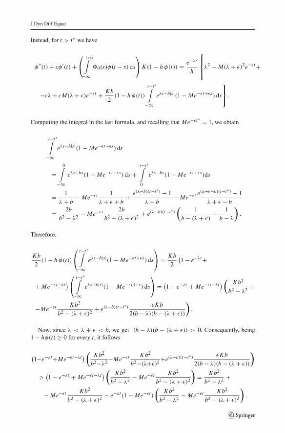
J Dyn Diff Equat

Instead, for t > t∗ we have

φ′′(t)+ cφ′(t)+⎛

⎝+∞∫

−∞�0(s)φ(t − s) ds

⎞

⎠ K (1 − h φ(t)) = e−λt

h

⎧⎪⎨

⎪⎩λ2 − M(λ+ ε)2e−εt+

−cλ+ cM(λ+ ε)e−εt + K b

2(1 − h φ(t))

t−t∗∫

−∞eλs−b|s|(1 − Me−εt+εs) ds

⎫⎬

⎭.

Computing the integral in the last formula, and recalling that Me−εt∗ = 1, we obtain

t−t∗∫

−∞eλs−b|s|(1 − Me−εt+εs) ds

=0∫

−∞eλs+bs(1 − Me−εt+εs) ds +

t−t∗∫

0

eλs−bs(1 − Me−εt+εs)ds

= 1

λ+ b− Me−εt 1

λ+ ε + b+ e(λ−b)(t−t∗) − 1

λ− b− Me−εt e(λ+ε−b)(t−t∗) − 1

λ+ ε − b

= 2b

b2 − λ2 − Me−εt 2b

b2 − (λ+ ε)2+ e(λ−b)(t−t∗)

(1

b − (λ+ ε)− 1

b − λ

).

Therefore,

K b

2(1 − h φ(t))

⎛

⎝t−t∗∫

−∞eλs−b|s|(1 − Me−εt+εs) ds

⎞

⎠ = K b

2

(1 − e−λt+

+ Me−εt−λt )⎛

⎝t−t∗∫

−∞eλs−b|s|(1 − Me−εt+εs) ds

⎞

⎠ = (1 − e−λt + Me−εt−λt )(

K b2

b2 − λ2 +

−Me−εt K b2

b2 − (λ+ ε)2+ e(λ−b)(t−t∗) εK b

2(b − λ)(b − (λ+ ε))

).

Now, since λ < λ + ε < b, we get (b − λ)(b − (λ + ε)) > 0. Consequently, being1 − hφ(t) ≥ 0 for every t , it follows

(1−e−λt+Me−εt−λt )

(K b2

b2−λ2 −Me−εt K b2

b2−(λ+ε)2 +e(λ−b)(t−t∗) εK b

2(b − λ)(b − (λ+ ε))

)

≥ (1 − e−λt + Me−εt−λt )(

K b2

b2 − λ2 − Me−εt K b2

b2 − (λ+ ε)2

)= K b2

b2 − λ2 +

− Me−εt K b2

b2 − (λ+ ε)2− e−λt (1 − Me−εt )

(K b2

b2 − λ2 − Me−εt K b2

b2 − (λ+ ε)2

).

123

J Dyn Diff Equat

Since 1b2−λ2 ≤ 1

b2−(λ+ε)2 and 0 ≤ 1 − Me−εt ≤ 1 for t > t∗, we have

e−λt (1 − Me−εt )

(K b2

b2 − λ2 − Me−εt K b2

b2 − (λ+ ε)2

)

≤ e−λt (1 − Me−εt )2(

K b2

b2 − (λ+ ε)2

)≤ e−λt K b2

b2 − (λ+ ε)2.

Finally,

(1−e−λt+Me−εt−λt)

(K b2

b2−λ2 −Me−εt K b2

b2 − (λ+ ε)2+e(λ−b)(t−t∗) εK b

2(b − λ)(b−(λ+ε)))

≥ K b2

b2 − λ2 − Me−εt K b2

b2 − (λ+ ε)2− e−λt K b2

b2 − (λ+ ε)2.

Hence, we get

λ2 − M(λ+ ε)2e−εt − cλ+ cM(λ+ ε)e−εt + K b

2(1 − h φ(t))

⎛

⎝t−t∗∫

−∞eλs−b|s|(1+

− Me−εt+εs) ds

⎞

⎠ ≥ λ2 − M(λ+ ε)2e−εt − cλ+ cM(λ+ ε)e−εt + K b2

b2 − λ2 +

− Me−εt K b2

b2 − (λ+ ε)2− e−λt K b2

b2 − (λ+ ε)2= λ2 − cλ+ K b2

b2 − λ2 +

−Me−εt((λ+ ε)2 − c(λ+ ε)+ K b2

b2 − (λ+ ε)2

)− e−λt K b2

b2 − (λ+ ε)2

= Q(λ)− Me−εt Q(λ+ ε)− e−λt K b2

b2 − (λ+ ε)2,

where Q(s) := s2 − cs + K b2

b2−s2 .We claim that for a suitable choice of λ, ε and M the last term in the previous chain of

inequalities is non-negative. Indeed, notice that Q(0) = K . Moreover, conditions b > 2√

Kand (5.17) imply that c < 2b and Q(c/2) < 0. Consequently, there exist positive numbersλ = λ(c, b, K ), ε = ε(c, b, K ) satisfying ε < λ, λ+ ε < c/2, such that

Q(λ) = 0 and Q(λ+ ε) < 0. (5.19)

Moreover, since t > t∗ > 0, we have 0 < e−(λ−ε)t < 1, so

Q(λ)− Me−εt Q(λ+ ε)− e−λt K b2

b2 − (λ+ ε)2= e−εt [−M Q(λ+ ε) +

− e−(λ−ε)t K b2

b2 − (λ+ ε)2

]≥ e−εt

[−M Q(λ+ ε)− K b2

b2 − (λ+ ε)2

]≥ 0

provided that M > 0 is large enough.Therefore, with the above choice of λ, ε,M = M(b, K , λ, ε) = M(c, b, K ), the function

φ(t) = max{0, 1h (1 − Me−εt )e−λt } is a sub-solution.

In order to find a super-solution, consider the function

ψ(t) := min{1, e−λt }

123

J Dyn Diff Equat

where the constantλ > 0 is the same as above. Observe that 0 = ψ ′(0−) > ψ ′(0+), moreoverif t < 0 then ψ ′(t) = ψ ′′(t) = 0, and if t > 0 then ψ ′(t) = −λe−λt , ψ ′′(t) = λ2e−λt .

To show that ψ is a super-solution we have to prove that

ψ ′′(t)+ cψ ′(t)+⎛

⎝+∞∫

−∞�0(s)ψ(t − s) ds

⎞

⎠ f0(ψ(t))

≤ ψ ′′(t)+ cψ ′(t)+⎛

⎝+∞∫

−∞�0(s)ψ(t − s) ds

⎞

⎠ K (1 − ψ(t)) ≤ 0

for every t in R. Now, for t < 0 we have ψ ′′(t)+cψ ′(t)+( ∫ +∞

−∞ �0(s)ψ(t − s) ds)

K (1−ψ(t)) = 0.

Instead, for t > 0 we have

ψ ′′(t)+ cψ ′(t)+⎛

⎝+∞∫

−∞�0(s)ψ(t − s) ds

⎞

⎠ K (1 − ψ(t))

= λ2e−λt − cλe−λt + K (1 − e−λt )e−λt

+∞∫

−∞�0(s)e

λsds

= e−λt

⎛

⎝λ2 − cλ+ K (1 − e−λt )

+∞∫

−∞�0(s)e

λs ds

⎞

⎠ .

Since 0 ≤ 1 − e−λt ≤ 1 for t > 0, taking account of (5.19), we deduce

λ2 − cλ+ K (1 − e−λt )

+∞∫

−∞�0(s)e

λs ds ≤ λ2 − cλ+ Kb

2

+∞∫

−∞eλs−b|s| ds

= λ2 − cλ+ K b2

b2 − λ2 = Q(λ) = 0.

Then, the function ψ(t) is a super-solution.Finally, note that φ(t) < ψ(t) for every t ∈ R. In fact, this is trivial for t ≤ t∗, whereas

for every t ≥ t∗ we have

φ(t) = 1

h(1 − Me−εt )e−λt < e−λt = ψ(t).

Therefore, by applying Theorem 4.3 we deduce that the differential equation in (5.14)admits a decreasing solution u satisfying φ(t) ≤ u(t) ≤ ψ(t) for every t ∈ R. This immedi-ately implies that u(+∞) = 0. Finally, by arguing as in the proof of Theorem 5.2, one canprove that u(−∞) = 1 and the proof is complete. �

Similarly to what we done in the case of delayed equation, we present now an example ofapplication of the previous result.

123

J Dyn Diff Equat

Example 5.8 Let us consider the non-local reaction-diffusion equation

vτ (τ, x) = vxx (τ, x)+ K b

2(1 − v(τ, x))p

+∞∫

−∞e−b|x−σ |v(t, σ ) dσ, with p ≥ 1.

Put f0(s) := (1 − s)p , we can apply Theorem 5.7 and deduce the existence of travellingfronts.

Remark 5.9 As we mentioned in the Introduction, the classical Fisher–KPP equation with thereaction term f (u) = K u(1−u) can be viewed as a particular case of the equation governedby the convolution integral when the kernel is the Dirac delta function and can be obtainedtaking the limit as b → +∞. Notice that the threshold values c∗

1 = c∗1(b, K ), c∗

2 = c∗2(b, K )

given by (5.17) satisfy

limb→+∞ c∗

1(b, K ) = 2√

K and limb→+∞ c∗

2(b, K ) = +∞

in accordance with the circumstance that the classical Fisher–KPP equation in this case admitst.w.s. if and only if c ≥ c∗ = 2

√f ′(0) = 2

√K .

6 Final Discussion

First of all, we clarify that we limit ourselves to search for monotone fronts since whenconsidering functions takings values in [0, 1] they are the only possible solutions. In fact,if the functional F satisfies the rather natural condition that F(u)(t) ≥ 0 on R for everyfunction u taking values on [0, 1], it is easy to verify that each possible solution is monotonedecreasing. Indeed, if u′(t) > 0 for every t in some interval J ⊂ R, then c ≥ 0 by virtueof Proposition 3.2 and from Eq. (3.1) we derive that u′′(t) ≤ 0 for every t ∈ J , implyingthat u′(t) > 0 for every t ∈ (−∞, sup J ), in contradiction with the boundary conditionu(−∞) = 1.

Nevertheless, in some nondimensionalised model, the dynamic can also have non-mono-tone t.w.s., presenting a hump exceeding the value 1, as it is was shown in reference [6], bymeans of a formal asymptotic analysis. A biological interpretation of this phenomenon waspresented in reference [6] in the context of biological invasion. Indeed, when an invasionfront moves out, individuals at the front are in competition only with those behind themand so the population can get above the carrying capacity level, which is the maximum theenvironment can sustain in the long term.

Comparing with the wide literature and the deep study developed for classical (non-func-tional) reaction-diffusion equations, clearly this research is far from being complete, sincethere are still many open problems and various aspects should be clarified. First of all, thequestion of the uniqueness of the profiles. Indeed, in the classical case, it is well known thatfor every admissible wave speed c the profile is unique (up to a shift of the variable). We donot deal with this topic in the present paper and this question remains open. Secondly, in theclassical case the range C of the admissible wave speed is a closed half-line [c∗,+∞), whilein Proposition 4.5 we have just proved that it is a closed set and actually it is not clear whetherit is an interval (connected) and moreover whether it is unbounded. Perhaps the first questioncan be handled by using some comparison argument, whereas the possible unboundedness ismore delicate. Indeed, we have not any non-existence result and consequently we are neitherable to characterize the set C, nor able to prove that it is bounded. However, in the applications

123

J Dyn Diff Equat

presented in Sect. 5 (see Theorem 5.3, Theorem 5.7 and Remark 5.9) we have proved thatthe range C contains a compact interval whose right-hand extremum tends to +∞ when thefunctional model approaches (in some sense) the classical one.

References

1. Aronson, D.G., Weinberger, H.F.: Multidimensional nonlinear diffusion arising in population genet-ics. Adv. Math. 30, 33–76 (1987)

2. Faria, T., Trofimchuk, S.: Nonmonotone travelling waves in a single species reaction-diffusion equationwith delay. J. Differ. Equ. 228, 357–376 (2006)

3. Fife, P.C.: Mathematical Aspects of Reacting and Diffusing Systems, Lecture Notes in Biomathematics28. Springer, Berlin (1979)

4. Fisher, R.A.: The wave of advance of advantageous genes. Ann. Eugen. 7, 355–369 (1937)5. Gilding, B.H., Kersner, R.: Travelling Waves in Nonlinear Diffusion-Convection-Reaction. Birkhäuser,

Basel (2004)6. Gourley, S.A.: Travelling front solutions of a nonlocal Fisher equation. J. Math. Biol. 41, 272–284 (2000)7. Huang, J., Zou, X.: Existence of traveling wavefronts of delayed reaction diffusion systems without

monotonicity. Discr. Cont. Dyn. Syst. 9(4), 925–936 (2003)8. Huang, J., Zou, X.: Travelling wave solutions in delayed reaction diffusion systems with partial monoto-

nicity. Acta Math. Appl. Sin. 22(2), 243–256 (2006)9. Kamin, S., Rosenau, P.: Convergence to the travelling wave solution for a nonlinear reaction-diffusion

equation. Atti Accad. Naz. Lincei, Cl. Sci. Fis. Mat. Nat. IX. Ser. 15(3–4), 271–280 (2004)10. Kolmogorov, A.N., Petrovskii, I.G., Piskunov, N.S.: Étude de l’équation de la diffusion avec croissance

de la quantité de matière et son application à un problème biologique. Moscow Univ. Math. Bull. 1,1–25 (1937)

11. Ma, S.: Traveling wavefronts for delayed reaction-diffusion systems via a fixed point theorem. J. Differ.Equ. 171, 294–314 (2001)

12. Ma, S.: Traveling waves for non-local delayed diffusion equations via auxiliary equations. J. Differ.Equ. 237(2), 259–277 (2007)

13. Marcelli, C., Papalini, F.: Comparison results and existence of bounded solutions to strongly nonlinearsecond order differential equations. Top. Methods Nonlinear Anal. 34(1), 91–110 (2009)

14. Murray, J.D.: Mathematical Biology. Springer, Berlin (1993)15. So, J.W., Wu, J., Zou, X.: A reaction-diffusion model for a single species with age structure. I. Travel-

ling-wave fronts on unbounded domains. Proc. R. Soc. Lond. A 457, 1–13 (2001)16. Volpert, A., Volpert, V.: Travelling Wave Solutions of Parabolic Systems. Translation of Mathematical

Monograph, vol. 140. American Mathematical Society, Providence, RI (1994)17. Wu, J., Zou, X.: Traveling Wave Fronts of Reaction-Diffusion Systems with Delay. J. Dyn. Differ.

Equ. 13(3), 651–687 (2001)18. Wu, J., Zou, X.: Erratum: Traveling Wave Fronts of Reaction-Diffusion Systems with Delay. J. Dyn.

Differ. Equ. 20(2), 531–533 (2008)

123