a generalized likelihood ratio approach to the detection of jumps in linear systems min luo
TRANSCRIPT

A Generalized Likelihood Ratio A Generalized Likelihood Ratio Approach to the Detection of Approach to the Detection of
Jumps in Linear SystemsJumps in Linear Systems
Min Luo

OutlinesOutlines
Kalman filter GLR Adaptive filtering An example
FOR MORE INFO...
Alan S.Willsky, “A Generalized Likelihood Ratio Approach to the Detection and Estimation of Jumps in Linear System”, IEEE Transaction on Automatic Control, Feb, 1976
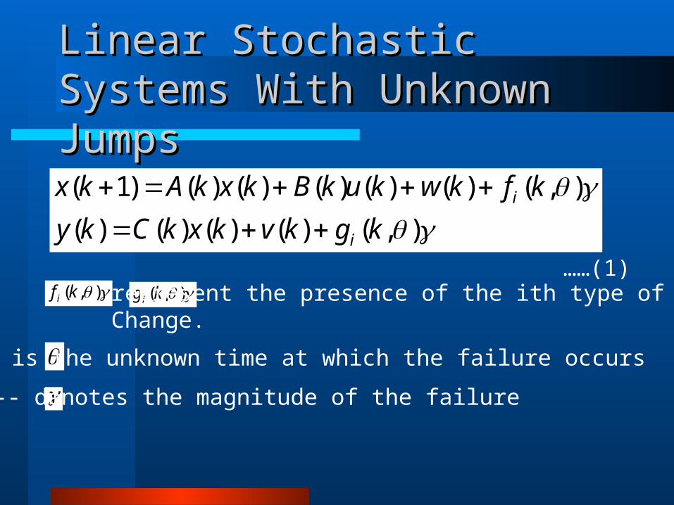
Linear Stochastic Systems With Linear Stochastic Systems With Unknown JumpsUnknown Jumps
),()()()()(
),()()()()()()1(
kgkvkxkCky
kfkwkukBkxkAkx
i
i
),(kf i ),(kg i represent the presence of the ith type of abruptChange.
--- is the unknown time at which the failure occurs
--- denotes the magnitude of the failure
……(1)

Kalman FilterKalman Filter
Design a Kalman filter based on normal operation:
)|1(ˆ)()1()1(
)1()1()|1(ˆ)1|1(ˆ
)()()|(ˆ)()|1(ˆ
kkxkCkykr
krkKkkxkkx
kukBkkxkAkkx
..….(2)
Kalman FilterKalman Filter
),()()(
),1()|1(ˆ)|1(ˆ
),()|(ˆ)|(ˆ
),()()(
kkrkr
kkkxkkx
kkkxkkx
kkxkx
iN
iN
iN
iN
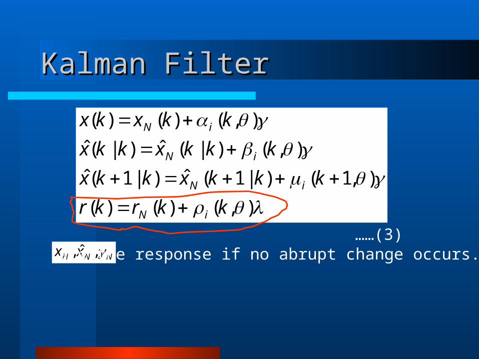
NNN xx ,ˆ, are the response if no abrupt change occurs.……(3)

Kalman FilterKalman Filter
),(),(),()(),(
),()(),1(
),(),1()1()1(
),1()1()1(),1(
),(),()(),1(
kgkkkCk
kkAk
kgkkCkK
kKCkKIk
kfkkAk
iiii
ii
ii
ii
iii
……(4)

Matched FilterMatched Filter
),()()( kkrkr iN
N --- zero-mean white Gaussian with covariance )(kV
Thus, we have a standard detection problem in white noise. Thesolution to this problem involves mathched filtering operation.
……(5)

Generalized Likelihood Ratio TestGeneralized Likelihood Ratio Test
We say that a test is a generalized likelihood ratio test for testing between hypotheses
g
00 : H 11 : Hand when
0
1)(ˆ 1
Nyg
)(ˆ)(ˆ
1
1N
N
y
ywhen
)(sup
)(sup)(ˆ
1
11
0
1
yp
ypy N
where
……(6)

Generalized Likelihood Ratio TestGeneralized Likelihood Ratio Test
))(ˆ(sup))](ˆ[(sup 1100
NN yPygE
Where the constant is such that
The precise optimal properties of the GLR test in thegeneral case are unknown, but for many special cases, the GLR test is optimal.
……(7)

Online GLROnline GLR
Compute the maximum likelihood estimates based onr(1),…, r(k) and the hypothesis H1.
)](ˆ,[)](ˆ,[)(ˆ 1 kkdkkCk
)(ˆ),(ˆ kk
……(8)

Online GLROnline GLR
),()(),(),,( 1'
jjVjikC i
k
ji
……(9)
),()(),(),,( 1'
jrjVjikd i
k
ji
Deterministic C:
Linear combination of residuals:

Online GLROnline GLR
The MLE )(ˆ k is the value k that maximizes
),(),(),(),,( 1' kdkCkdik
0
1
))(ˆ,(
H
H
kk
The decision rule is:
…(10)
…(11)

Online GLROnline GLR
• Data Window At any time , we restrict our optimization over to an interval of the form
k NkMk
We now consider the case in which we hypothesize if
--- an unknown scalar
},...,{ 1 Ni fff --- a given set of hypothesized “failure directions”

Online GLROnline GLR
is unknown, the GLR for this change is
),,(
),,(),,(
2
ika
ikbik
),,(),,(2),,( 2 ikaikbik
If
If is known, the likelihood of a type i change having occurred at time
…(12)

Online GLROnline GLR
ii fkCfika ),(),,( '
),(),,( ' kdfikb i
…(13)The decision as to the failure:
0
1
),,(
H
H
ik
…(14)

GLR Algorithm SummaryGLR Algorithm Summary
Kalman FilterKalman Filter
Matched FilterMatched Filter
Likelihood CalculationLikelihood Calculation
GLR Algorithm
Adaptive Filtering Adaptive Filtering
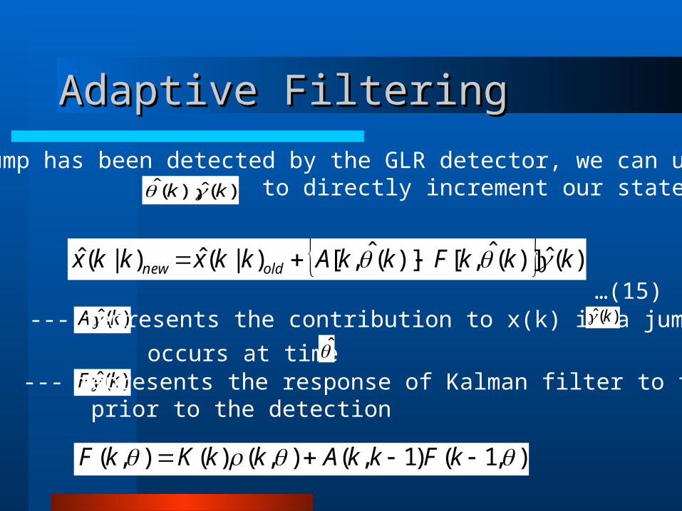
)(ˆ),(ˆ kk Once a jump has been detected by the GLR detector, we can useMLE’s to directly increment our state estimate.
)(ˆ)](ˆ,[)](ˆ,[)|(ˆ)|(ˆ kkkFkkAkkxkkx oldnew
),1()1,(),()(),( kFkkAkkKkF
)(ˆ kA --- represents the contribution to x(k) if a jump )(ˆ k
occurs at time )(ˆ kF --- represents the response of Kalman filter to the jump
prior to the detection
…(15)

Direct Compensation Direct Compensation
Kalm an F ilte rx
+
if
+
Cnewx
newy
S y s tem
+
_
y
rG L R
FAxx
Implementation of direct compensation technique

Some Comments of Adaptive Some Comments of Adaptive FilteringFilteringIncrease the estimation error covariance to reflect the degradation
in the quality of the estimate caused by the jump.
)](ˆ,[)](ˆ,[)](ˆ,[)](ˆ,[)](ˆ,[)|()|( 1 kkFkkAkkCkkFkkAkkPkkP oldnew
)](ˆ,[1 kkC is error covariance for )(ˆ k…(16)

Final IssueFinal Issue
Tradeoff between fast detection and accurate estimation of jump:
Different size of finite data window of GLR decides
• small --> accurate estimation of the jump• --> quick detection
)](ˆ,[1 kkC
)(ˆ kk

Detection Probability CalculationDetection Probability Calculation
The choice of a decision threshold and a window length requires the tradeoff among detection delay time, the Pf of the false alarm,and the of correct detection of a jump of magnitude at time .
),( vPD
dLHLlpP
dLHLlpP
D
F
)|(),(
)|(
,,1
0
…(17)

Apply GLR to a Tracking ProblemApply GLR to a Tracking Problem
The problem is to design a tracking filter which uses position measurements taken at 30s intervals to track the motion of a vehicle along a straight line.
10
1)1,(
tkkA
1
0B kjkj sftQjwkwE )/173.0())()(( 2
01C kjkj ftRjvkvE 2)600())()((

ExampleExample
The vehicle is subject to occasional step change of unknownmagnitude in either position or velocity. The tracking filter is a Kalman filter operating in steady state and requires 60-90 min to completely respond to such jumps.
The GLR system was implemented with the detection law:
6.10),(
0
1
H
H
k

ExampleExample
6,12 NM
6)(ˆ12 kkk
Jump identification is made at the first time the above formula is satisfied:
11)(ˆ kk
The optimization of is constrained to)(ˆ k
PF=0.005, PD>0.9

(a) Filter residuals for a 1320ftjump in position at 5 min
(b) Likelihood ratio for (a) using GLR

ConclusionConclusion
Develop an adaptive filtering technique for discrete-time linear stochastic systems subject to abrupt jumps in state variables.
The estimation system consists of Kalman filter and a detection-compensation system based on GLR testing.
Conclusion Conclusion
Once a jump is detected, we can adjust the filter in one of three ways:– Directly increment the state estimate– Increase the estimation error covariance and
thus allow the filter to adjust itself to the jump– Adjust both

Process Analysis and Abnormal Situation Detection:
From theory to Practice
ProblemProblem
Large volumes historical data The data are highly correlated The information stored in one variable is
small Measurements are often missing
on many variables

Possible SolutionPossible Solution
PCA PLS (projection to latent structures)
Outline:• Discusses the use of latent variable models• Multivariate statistical process monitoring• Abnormal situation detection• Fault diagnosis

Multivariate Nature of Fault Multivariate Nature of Fault DetectionDetection Univariate chart(Shewhart)
Problem:Most of the time the variables are notindependent of one another, and none of themadequately defines product quality by itself.
Multivariate chart

Separate Control Chart Per Separate Control Chart Per VariableVariable

Statistical Process ControlVersus Statistical Quality Control
Statistical quality control (SQC) One can ignore the hundreds of
process variables that are measured much more frequently than the product quality data.
Statistical process control (SPC) One must look at all the process
data as well.

Statistical Process ControlStatistical Process Control
Advantage of monitoring process data:Easier to diagnose the source of the
problemQuality data may not be available at
certain stages of the process

Latent Variables
These variables are highly correlated and theeffective dimension of the space in which theymove is very small (usually less than ten).
Consider the historical process data to consistof an (n by k ) matrix of process variablemeasurements X and a corresponding ( n by k)matrix of product quality data Y.

Latent VariablesLatent Variables
ETPX '
FTQY '
T is (n by A) matrix of latent variable scores.P(k by A), Q(m by A) are loading matrices that show how latent variables are related to X, Y variables.
Advantage:By working in this low-dimensional space of the latentvariables, the problems of process analysis, monitoring and optimization are greatly simplified.

Latent Variable MethodsLatent Variable Methods
PCA PLS Reduced rank regression (RRR) Canonical variate analysis(CCR) or
Canonical correlation regression (CVR)

Exploration and Analysis of Process Databases
By examining the behavior of the process data
in the projection spaces defined by the smallnumber of latent variables, regions of stableoperation, sudden changes, or slow processdrifts may be readily observed.

Checking Data Quality for Process Modeling
Identify outliers, check data for clusters Select data for the training part of
multivariate control charts

Process Monitoring and Fault Diagnosis
A model is built to relate X and Y using available historical or specially collected data. Monitoring charts are then constructed for future values of X.
Two complementary multivariate control chartsfor process monitoring :
1. Hotelling’s T2 chart

T2 Chart
A
i t
iA
is
tT
12
22
itsis the estimated variance of the corresponding latent variable.
This chart will check if a new observation vector of measurements on k process variables projects on the hyperplane within the limits determined by the reference data.

SPEX Chart
2. SPEx chart
2
1,, )ˆ(
k
iinewinew xxSPEx
is computed from the reference PLS or PCA model.inewx ,ˆ
This latter plot will detect the occurrence of any new events that cause the process to move away from the hyperplane defined by the reference model.
Fault DiagnosisFault Diagnosis
PLS or PCA models are used to construct themultivariate charts, they provide the user withthe capacity for diagnosing assignable causes.
Contribution plots are used to detect variablesresponsible for an out-of-control signal onSPEx ,T2.

Three Charts for Multivariate Process Monitoring

Troubleshooting and Monitoringof Batch Processes–
three-dimensional data arrayX(n by k by L)
k process variables are measured at L time intervalsfor each of n batches.

Multiway Extensions of PCA/ PLS
The matrix is unfolded into a two-dimensionalarray such that each row corresponds to a batch.
Mean centering of the variables effectively subtracts the trajectory, thus converting a nonlinear problemto one that can be tackled with linear methods such as PCA and PLS.

Multiway Extensions of PCA/ PLS
plot the loadings of each variable, for each time interval,for the first principal component of a PCA analysis wherethe batch data are unfolded.

the scores of the first two principal components for 61 completed batches

Online SPC Charts
When data are available in a historical database on many past normal batches, multivariate PCA and PLS models can be developed to establish online SPC charts for monitoring the progress of each new batch.

Online SPC Charts
Online monitoring of batch 56

Startup and Grade Transition Problems Process transitions are very frequent These transitions lead to problems The use of multivariate statistical
methods can improve process transitions

Multivariate Sensor and ImageAnalysis for Online Monitoring Similar banks of multivariate sensors
and color imaging cameras are used online to monitor and control industrial processes.
How to handle the huge amount of highly correlated data collected from these sensors and how to efficiently extract the subtle information contained in the data.

Observability/Detectability of FaultsThe model should be tested with
known faults to determine the “observability” of these faults.– SPE chart and the Hotelling’s T2 at A
components are used to monitor the process.
– If not both models signal the problem.– It needs more represented variable or it
requires that certain process variables be given a higher weight in the model.

Frequency of Sampling
For model building, it is important that the model is built with data collected with the same sampling frequency as will be used for the online operation of the model.
The choice of the monitoring interval also depends on how quickly the faults we are trying to detect manifest themselves.

Soft Sensors/Inferential Models
Soft sensors can either replace the hardware
sensor or be used in parallel with it to provide redundancy and verify whether the hardware sensor is drifting or has failed.
These inferential models are usually built by fitting either empirical or theoretically based models to plant data.

Using empirical models for soft sensors, latent variable models such as PLS offer some important advantages over standard regression models or neural networks.

Concluding Remarks
The use of latent variable model for extracting useful information from historical databases.
Wide acceptance in industry, particularly for the problems of process analysis, monitoring, and soft sensors.