Geosci. Model Dev., 6, 1977–1988, 2013www.geosci-model-dev.net/6/1977/2013/doi:10.5194/gmd-6-1977-2013© Author(s) 2013. CC Attribution 3.0 License.

GeoscientificModel Development

Open A

ccess

A generic biogeochemical module for Earth system models:Next Generation BioGeoChemical Module (NGBGC), version 1.0

Y. Fang1, M. Huang2, C. Liu3, H. Li 1, and L. R. Leung2

1Hydrology Group, Energy and Environment Directorate, Pacific Northwest National Laboratory, Richland, WA 99352, USA2Climate Physics Group, Fundamental and Computational Sciences Directorate, Pacific Northwest National Laboratory,Richland, WA 99352, USA3Geochemistry Group, Fundamental and Computational Sciences Directorate, Pacific Northwest National Laboratory,Richland, WA 99352, USA

Correspondence to:Y. Fang (yilin.fang@pnnl.gov)

Received: 22 April 2013 – Published in Geosci. Model Dev. Discuss.: 13 June 2013Revised: 18 September 2013 – Accepted: 30 September 2013 – Published: 13 November 2013

Abstract. Physical and biogeochemical processes regulatesoil carbon dynamics and CO2 flux to and from the atmo-sphere, influencing global climate changes. Integration ofthese processes into Earth system models (e.g., communityland models (CLMs)), however, currently faces three ma-jor challenges: (1) extensive efforts are required to modifymodeling structures and to rewrite computer programs to in-corporate new or updated processes as new knowledge isbeing generated, (2) computational cost is prohibitively ex-pensive to simulate biogeochemical processes in land mod-els due to large variations in the rates of biogeochemicalprocesses, and (3) various mathematical representations ofbiogeochemical processes exist to incorporate different as-pects of fundamental mechanisms, but systematic evaluationof the different mathematical representations is difficult, ifnot impossible. To address these challenges, we propose anew computational framework to easily incorporate phys-ical and biogeochemical processes into land models. Thenew framework consists of a new biogeochemical module,Next Generation BioGeoChemical Module (NGBGC), ver-sion 1.0, with a generic algorithm and reaction database sothat new and updated processes can be incorporated into landmodels without the need to manually set up the ordinary dif-ferential equations to be solved numerically. The reactiondatabase consists of processes of nutrient flow through theterrestrial ecosystems in plants, litter, and soil. This frame-work facilitates effective comparison studies of biogeochem-ical cycles in an ecosystem using different conceptual modelsunder the same land modeling framework. The approach was

first implemented in CLM and benchmarked against simu-lations from the original CLM-CN code. A case study wasthen provided to demonstrate the advantages of using the newapproach to incorporate a phosphorus cycle into CLM. Toour knowledge, the phosphorus-incorporated CLM is a newmodel that can be used to simulate phosphorus limitation onthe productivity of terrestrial ecosystems. The method pre-sented here could in theory be applied to simulate biogeo-chemical cycles in other Earth system models.

1 Introduction

Terrestrial ecosystems store almost three times as much car-bon as the atmosphere; hence changes in the terrestrial car-bon budgets have important implications for the future cli-mate through carbon cycle feedbacks. Accurate modeling ofcarbon cycling at regional to global scales must incorporatemechanism-based, robust representations of soil carbon andnutrient cycling processes as well as other biogeochemicalprocesses that are coupled with the carbon cycle.

A number of biogeochemistry modules have been devel-oped and used in Earth system models (ESMs) to simulatethe fluxes of carbon, nitrogen, energy, and water into andout of an ecosystem (e.g., CLM-CN, which originated fromBiome-BGC (Thornton et al., 2007), CENTURY/DAYCENT(Parton et al., 2001, 1988), and other terrestrial biospheremodels that participated in the Carbon Land Model Inter-comparison Project (CLAMP) (Randerson et al., 2009), the

Published by Copernicus Publications on behalf of the European Geosciences Union.

1978 Y. Fang et al.: A generic biogeochemical module for Earth system models

International Land Model Benchmarking Project (ILAMB)(Luo et al., 2012), etc.). In these previous modules, bio-geochemical processes are represented by a set of ordinarydifferential equations (ODEs), and each of the equations isa sum of the contributions from various individual biogeo-chemical processes. Although schematic diagrams are pre-sented in the literature for C and N flows among differentcompartments, e.g., within the plants, above ground or in thesoil, it is difficult to deconvolute each differential equation totrack the contribution from individual processes. Not know-ing the detailed processes simulated in a model makes it dif-ficult to update or add new processes to the module. Further-more, many land surface models such as the current CLMonly include C and N cycling, even though P cycling has beenshown to be important in regulating terrestrial biogeochemi-cal processes (Buendia et al., 2010; Goll et al., 2012; Wanget al., 2010; Yang et al., 2013). In addition, anthropogenicsulfur (S), which is not included in the current CLM, canalso disturb the biogeochemical cycling in terrestrial ecosys-tems through competition for labile forms of organic car-bon between nitrate-reducing and sulfate-reducing bacteria(Bünemann and Condron, 2007; Gu et al., 2012). AlthoughP models and S models have been developed in the literature(Bünemann and Condron, 2007; Goll et al., 2012; Mitchelland Fuller, 1988; Wang et al., 2010), including them in CLMin its current code structure requires a nontrivial amount ofwork.

All of the biogeochemistry modules, as reviewed in arecent report of the Intergovernmental Panel on ClimateChange (IPCC, 2007), assume that organic carbon decompo-sition driven by microbial communities follows a first-orderchemical decay process, neglecting feedback interactions be-tween microbial activities and the controlling processes andfactors such as the form of substrates, microbial function,community, and abundance (Todd-Brown et al., 2012). Thephysiology of microbial communities is affected by climatechange, which in turn leads to changes in microbial decom-position rates (Bradford et al., 2008). To better representhow microbial processes influence biogeochemical cycling,integrating microbial communities into terrestrial ecosystemmodels has been called upon in recent years to reduce un-certainty in model prediction (Allison and Martiny, 2008;McGuire and Treseder, 2010). Recent advances in soil mi-crobiology are now allowing us to better understand the dy-namics of microbial communities and how they affect bio-geochemical processes in soils. The simple representationof soil biogeochemical processes in current models can nolonger handle the complexity that results from the integra-tion of microbial community dynamics.

One of the major challenges of integrating microbial dy-namics is that currently each biogeochemistry module is de-veloped in an ad hoc way with little flexibility to modify orincorporate new biogeochemical processes because they arehardwired in the computer source codes. When additionaland/or different biogeochemical and physical processes are

to be included, the source codes have to be significantly mod-ified, including code changes to output new state variables.For example, a recent modeling study has found that incor-porating microbial processes can improve the global soil car-bon projections (Wieder et al., 2013). The modeled processesin that study are compared to the conventional processes inFig. 1. It can be seen that in order to use this simple newmodel, ODEs for carbon state variables in litter and soil haveto be manually modified and six more ODEs for the microbeshave to be added. Users have to manually discern the ODEsand keep track of the state variables, stoichiometries, andtheir relationship to each process. This is easy when fluxesbetween different pools only pass through a single microbialpopulation, but in reality the conversion of pools involvesmicrobial consortia. It is tractable when each process onlyinvolves at most two state variables as currently representedin CLM, although a significant effort is required to track eachvariable and process. It becomes a significant burden for theprogrammers and modelers when complex reaction pathwaysthat involve more variables and processes have to be inte-grated. Users also need to be familiar with the code beforethey can make efficient updates to it. Maintenance and modi-fication of the current software hierarchy is time consuming,labor intensive, and error prone. These difficulties can be re-solved using the new biogeochemical module presented inthis study.

In this paper, we propose a generic, reaction-based algo-rithm to integrate soil biogeochemical processes into landsurface models using processes simulated in CLM as an ex-ample. CLM is a land model driven by atmospheric forc-ing. It simulates coupled biogeophysical and biogeochemicalprocesses, which include solar and longwave radiation inter-actions with vegetation canopy and soil, momentum and tur-bulent fluxes from canopy and soil, heat transfer in soil andsnow, canopy hydrology, soil hydrology, snow hydrology,stomatal physiology and photosynthesis, river transport, andcarbon–nitrogen cycling that includes prognostic vegetationphenology (Lawrence et al., 2011). The carbon–nitrogen bio-geochemical module in CLM is referred to as CLM-CN. It isbased on the terrestrial biogeochemistry Biome-BGC modelwith a prognostic carbon and nitrogen cycle (Thornton et al.,2002; Thornton and Rosenbloom, 2005). In CLM-CN, thephotosynthetic carbon is partitioned into vegetation pools. Itsimulates a total of around 100 state variables in plant poolsfor leaf, live stem, dead stem, live coarse root, dead coarseroot, fine root, growth storage pools for leaf and fine rootgrowth, a coarse woody debris pool, three litter pools andfour soil pools. Hundreds of physical and biogeochemicalprocesses are used to represent the carbon and nitrogen cy-cles. The equation of the conservation of carbon and nitrogenmass in each pool is solved using an explicit method, i.e., thestate of a system at a later time is calculated from the state ofthe system at the current time. Detailed technical descriptionof the model can be found in Oleson et al. (2010).

Geosci. Model Dev., 6, 1977–1988, 2013 www.geosci-model-dev.net/6/1977/2013/

Y. Fang et al.: A generic biogeochemical module for Earth system models 1979

Fig. 1. Diagram of soil C models.(a) Conventional model and(b) microbial model. Lit, SOM, and Mic stand for C pools for litter,soil organic, and microbial biomass, respectively. Dashed arrowsare plant inputs. Solid arrows are fluxes between pools.

The new biogeochemical module developed in this papercan be readily used to update or incorporate new C, N, Pand other nutrient cycle models into CLM and other Earthsystem models and to evaluate the effects of alternative pro-cess pathways and mechanisms on climate changes. Similarto modeling geochemical reactions using the reaction-basedapproach that has been commonly used in modeling subsur-face reactive transport (Aguilera et al., 2005; Chilakapati etal., 2000; Yeh et al., 2001), the new biogeochemical mod-ule treats terrestrial C, N, and P cycles as reaction pathwaysand these pathways are explicitly modeled using the reaction-based approach. The reaction-based approach requires a self-consistent reaction network, the forming of which with cor-rect stoichiometries is a major challenge not only for mod-eling, but also for process characterization and understand-ing because of the complexity and a large number of biogeo-chemical processes and reactions involved in terrestrial car-bon cycling. To solve this problem from the modeling pointof view, a reaction database that can be used to conciselystore all biogeochemical reactions in plants, litter, and soil

that can potentially affect carbon cycling processes is devel-oped here. In the following sections, we will first introducethe reaction-based approach, followed by using this approachto develop the generic biogeochemical module in CLM. Asa validation, the results from the new module incorporatedinto CLM were compared with the original CLM-CN. Theresults were then compared to those using the decompositionmodel of soil organic matter in CENTURY (Parton et al.,1988) under the CLM modeling framework. A procedure tointegrate new processes into the new biogeochemical moduleis demonstrated using global P cycling as an example (Wanget al., 2010). The model that includes the phosphorus dynam-ics can be used to evaluate the effect of phosphorus on pro-ductivity of terrestrial ecosystems.

2 Methods

2.1 Reaction-based approach

A dynamic reaction system may be defined by reaction path-ways or networks (Yeh et al., 2001). In the reaction-basedapproach, the mass balance of each state variable of the reac-tion system can be written as

d Ci

dt=

N∑k=1

(νik − µik)Rk, (1)

in whichCi is the mass of theith state variable,t is time,Rk

is the rate of thekth reaction,vik is the reaction stoichiometryof the ith state variable in thekth reaction associated withthe products,µik is the reaction stoichiometry of theith statevariable in thekth reaction associated with the reactants, andN is the number of reactions. Equation (1) states that therate of change in the mass of any state variable is due to allreactions that produce or consume that state variable. Thewhole system can be written in a matrix form as

[I ]{

dC

dt

}= [A] {R} . (2)

If M is the total number of state variables in the system,

then [I ] is anM × M unit matrix,{

dCdt

}is a vector of length

M, and [A] is anM×N matrix, the columnk of which con-sists of stoichiometries of allC

′

is involved in reactionk withrateRk, which are allowed to vary during the simulation toaccount for the effects of moisture, temperature, etc. on thereaction stoichiometries.

The reaction rates in subsurface ecosystems typically spana wide range of magnitude, which makes it inefficient todirectly integrate Eq. (1). To overcome this difficulty, thefast reactions are often assumed to occur instantaneously, sothe ODEs for the fast reactions can then be described us-ing thermodynamic equilibrium approaches represented byalgebraic equations (AEs). Automatic code generators are al-ready available to serve this purpose (Aguilera et al., 2005;

www.geosci-model-dev.net/6/1977/2013/ Geosci. Model Dev., 6, 1977–1988, 2013

1980 Y. Fang et al.: A generic biogeochemical module for Earth system models

Chilakapati et al., 2000). However, many of them dependon third-party commercial software. In this paper, we usea systematic way to derive ODEs and decouple them fromfast reactions using matrix row and column operation (ma-trix decomposition) as detailed in Fang et al. (2003). A sim-ple system with one slow reaction and one fast (equilibrium)reaction, and three state variables are used to illustrate themethod:

aA ↔ bB, R1 (R1)

and

A ↔ cC, R2. (R2)

We define the flux of a substance as a derivative of thatsubstance with respect to time, and it has the dimension ofamount of substance per unit volume transformed per unittime. The reaction rate for a single reaction differs from theflux of a substance by the reciprocal of its stoichiometricnumber in that reaction. The rate of a reaction is alwayspositive, and it can be calculated either as linear or non-linear function. Assuming Reaction (R1) is a slow reactionwith reaction rateR1 and Reaction (R2) is a fast adsorp-tion/desorption reaction with reaction rateR2, the simple sys-tem in matrix form can be written as1 0 0

0 1 00 0 1

dAdtdBdtdCdt

=

−a −1b 00 c

{R1R2

}. (3)

Equation (3) can be expanded as

dA

dt= −aR1 − R2, (4)

dB

dt= bR1 (5)

anddC

dt= cR2. (6)

Direct integration of the above ODEs is impractical dueto the large rate ofR2, which requires very small time steps.To solve the problem, a direct thermodynamic equilibriumapproach, such as a sorption isotherm (Wang et al., 2010),may be employed to model the fast Reaction (R2). The sys-tem can now be solved with two ODEs and one algebraicequation andR2 is no longer in any of the ODEs. This canbe done by performing column reduction by determining apivot (nonzero) element in the fast reaction column in matrix[A] of Eq. (2) and using a matrix row operation to convertthe column containing the pivot element into a unit column.Element–1 or c in the second column of the reaction matrixin Eq. (3) can be a pivot element. Ifc is chosen as a pivotelement, the third row of the matrix equation is first dividedby c and then added to the first row to convert the second col-umn of the reaction matrix into a unit column. Equation (3)now becomes1 0 1

c

0 1 00 0 1

c

dAdtdBdtdCdt

=

−a 0b 00 1

{R1R2

}. (7)

Fig. 2.Diagram of model structure. Rectangles represent model in-put/output, ovals represent executable programs.

Expanding Eq. (7), we obtain the following:

d(A + 1/cC)

dt= −aR1, (8)

dB

dt= bR1 (9)

anddC

dt= cR2. (10)

Equation (10) is the only ODE that containsR2 and it canbe replaced with an algebraic equation (which can be a func-tion of A and C) and solved together with Eqs. (8) and (9). Aand C can be solved using Newton–Raphson iteration after(A+1/cC) is solved with explicit time integration.

If the system contains no fast processes, ODEs can beformed by simply expanding the matrix equation providedby the user. Otherwise, column reduction will be performedto generate ODEs containing only slow reactions similar tothe procedure above for the simple example. The equationscan be solved either using an explicit method or the Newton–Raphson iteration approach. The solver developed in Fang etal. (2003) was modified and is called NGBGC (Next Gener-ation BioGeoChemical Module) hereafter in this study.

2.2 Development of the generic biogeochemicalmodule

The new biogeochemical module, NGBGC, is designed toflexibly handle any number of biogeochemical processes andstate variables that are to be included in any ESM withoutchanging algorithms and codes related to ODEs for biogeo-chemistry in CLM. In addition, NGBGC can be convenientlyused to derive the mathematical equations to describe theseprocesses. A conceptual diagram in Fig. 2 shows the pro-cedure from preparing input (steps above the dotted line) torunning NGBGC inside CLM. The preprocessing part runs aPERL script on a reaction network written in a text file. ThePERL script generates reaction stoichiometry and supporting

Geosci. Model Dev., 6, 1977–1988, 2013 www.geosci-model-dev.net/6/1977/2013/

Y. Fang et al.: A generic biogeochemical module for Earth system models 1981

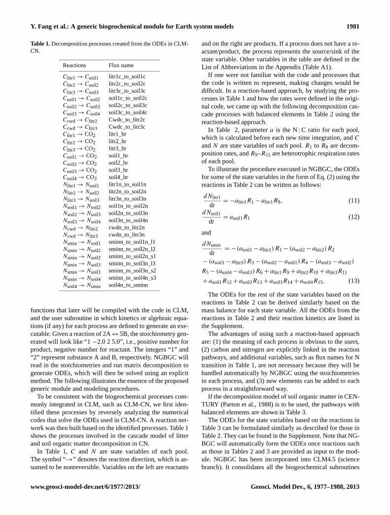
Table 1.Decomposition processes created from the ODEs in CLM-CN.

Reactions Flux name

Clitr1 → Csoil1 litr1c_to_soil1cClitr2 → Csoil2 litr2c_to_soil2cClitr3 → Csoil3 litr3c_to_soil3cCsoil1 → Csoil2 soil1c_to_soil2cCsoil2 → Csoil3 soil2c_to_soil3cCsoil3 → Csoil4 soil3c_to_soil4cCcwd → Clitr2 Cwdc_to_litr2cCcwd → Clitr3 Cwdc_to_litr3cClitr1 → CO2 litr1_hrClitr2 → CO2 litr2_hrClitr3 → CO2 litr3_hrCsoil1 → CO2 soil1_hrCsoil2 → CO2 soil2_hrCsoil3 → CO2 soil3_hrCsoil4 → CO2 soil4_hrNlitr1 → Nsoil1 litr1n_to_soil1nNlitr2 → Nsoil2 litr2n_to_soil2nNlitr3 → Nsoil3 litr3n_to_soil3nNsoil1 → Nsoil2 soil1n_to_soil2nNsoil2 → Nsoil3 soil2n_to_soil3nNsoil3 → Nsoil4 soil3n_to_soil4nNcwd → Nlitr2 cwdn_to_litr2nNcwd → Nlitr3 cwdn_to_litr3nNsmin→ Nsoil1 sminn_to_soil1n_l1Nsmin→ Nsoil2 sminn_to_soil2n_l2Nsmin→ Nsoil2 sminn_to_soil2n_s1Nsmin→ Nsoil3 sminn_to_soil3n_l3Nsmin→ Nsoil3 sminn_to_soil3n_s2Nsmin→ Nsoil4 sminn_to_soil4n_s3Nsoil4 → Nsmin soil4n_to_sminn

functions that later will be compiled with the code in CLM,and the user subroutine in which kinetics or algebraic equa-tions (if any) for each process are defined to generate an exe-cutable. Given a reaction of 2A↔ 5B, the stoichiometry gen-erated will look like “1−2.0 2 5.0”, i.e., positive number forproduct, negative number for reactant. The integers “1” and“2” represent substance A and B, respectively. NGBGC willread in the stoichiometries and run matrix decomposition togenerate ODEs, which will then be solved using an explicitmethod. The following illustrates the essence of the proposedgeneric module and modeling procedures.

To be consistent with the biogeochemical processes com-monly integrated in CLM, such as CLM-CN, we first iden-tified these processes by reversely analyzing the numericalcodes that solve the ODEs used in CLM-CN. A reaction net-work was then built based on the identified processes. Table 1shows the processes involved in the cascade model of litterand soil organic matter decomposition in CN.

In Table 1,C and N are state variables of each pool.The symbol “→” denotes the reaction direction, which is as-sumed to be nonreversible. Variables on the left are reactants

and on the right are products. If a process does not have a re-actant/product, the process represents the source/sink of thestate variable. Other variables in the table are defined in theList of Abbreviations in the Appendix (Table A1).

If one were not familiar with the code and processes thatthe code is written to represent, making changes would bedifficult. In a reaction-based approach, by studying the pro-cesses in Table 1 and how the rates were defined in the origi-nal code, we came up with the following decomposition cas-cade processes with balanced elements in Table 2 using thereaction-based approach.

In Table 2, parametera is the N: C ratio for each pool,which is calculated before each new time integration, andC

andN are state variables of each pool.R1 to R8 are decom-position rates, andR9–R15 are heterotrophic respiration ratesof each pool.

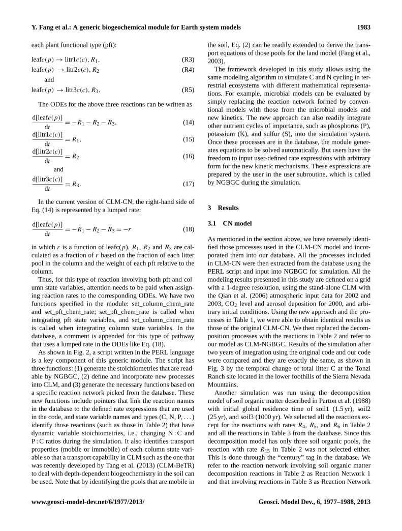
To illustrate the procedure executed in NGBGC, the ODEsfor some of the state variables in the form of Eq. (2) using thereactions in Table 2 can be written as follows:

dNlitr1

dt= −alitr1R1 − alitr1R9, (11)

dNsoil1

dt= asoil1R1 (12)

and

dNsmin

dt= −(asoil1− alitr1)R1 − (asoil2− alitr2)R2

− (asoil3− alitr3)R3 − (asoil2− asoil1)R4 − (asoil3− asoil2)

R5 − (asoil4− asoil3)R6 + alitr1R9 + alitr2R10+ alitr3R11

+ asoil1R12+ asoil2R13+ asoil3R14+ asoil4R15. (13)

The ODEs for the rest of the state variables based on thereactions in Table 2 can be derived similarly based on themass balance for each state variable. All the ODEs from thereactions in Table 2 and their reaction kinetics are listed inthe Supplement.

The advantages of using such a reaction-based approachare: (1) the meaning of each process is obvious to the users,(2) carbon and nitrogen are explicitly linked in the reactionpathways, and additional variables, such as flux names for Ntransition in Table 1, are not necessary because they will behandled automatically by NGBGC using the stoichiometriesin each process, and (3) new elements can be added to eachprocess in a straightforward way.

If the decomposition model of soil organic matter in CEN-TURY (Parton et al., 1988) is to be used, the pathways withbalanced elements are shown in Table 3.

The ODEs for the state variables based on the reactions inTable 3 can be formulated similarly as described for those inTable 2. They can be found in the Supplement. Note that NG-BGC will automatically form the ODEs once reactions suchas those in Tables 2 and 3 are provided as input to the mod-ule. NGBGC has been incorporated into CLM4.5 (sciencebranch). It consolidates all the biogeochemical subroutines

www.geosci-model-dev.net/6/1977/2013/ Geosci. Model Dev., 6, 1977–1988, 2013

1982 Y. Fang et al.: A generic biogeochemical module for Earth system models

Table 2.CLM-CN decomposition cascade model.

Reactions Rate

(asoil1–alitr1) Nsminn+ Clitr1+ alitr1 Nlitr1 → Csoil1+ asoil1 Nsoil1 R1(asoil2–alitr2) Nsminn+ Clitr2+ alitr2 Nlitr2 → Csoil2+ asoil2 Nsoil2 R2(asoil3–alitr3) Nsminn+ Clitr3+ alitr3 Nlitr3 → Csoil3+ asoil3 Nsoil3 R3(asoil2–asoil1) Nsminn+ Csoil1+ asoil1 Nsoil1 → Csoil2+ asoil2 Nsoil2 R4(asoil3–asoil2) Nsminn+ Csoil2+ asoil2 Nsoil2 → Csoil3+ asoil3 Nsoil3 R5(asoil4–asoil3) Nsminn+ Csoil3+ asoil3 Nsoil3 → Csoil4+ asoil4 Nsoil4 R6Ccwd+ acwd Ncwd → Clitr2+ acwd Nlitr2 R7Ccwd+ acwd Ncwd → Clitr3+ acwd Nlitr3 R8Clitr1+ alitr1 Nlitr1 → CO2+ alitr1 Nsmin R9Clitr2+ alitr2 Nlitr2 → CO2+ alitr2 Nsmin R10Clitr3+ alitr3 Nlitr3 → CO2+ alitr3 Nsmin R11Csoil1+ asoil1 Nsoil1 → CO2+ asoil1 Nsmin R12Csoil2+ asoil2 Nsoil2 → CO2+ asoil2 Nsmin R13Csoil3+ asoil3 Nsoil3 → CO2+ asoil3 Nsmin R14Csoil4+ asoil4 Nsoil4 → CO2+ asoil4 Nsmin R15

Table 3.CENTURY decomposition model of soil organic matter.

Reactions Rate

(asoil2–asoil1) Nsmin+ Csoil1+ asoil1 Nsoil1 → Csoil2+ asoil2 Nsoil2 R1(asoil3–asoil1) Nsmin+ Csoil1+ asoil1 Nsoil1 → Csoil3+ asoil3 Nsoil3 R2(asoil1–asoil2) Nsmin+ Csoil2+ asoil2 Nsoil2 → Csoil1+ asoil1 Nsoil1 R3(asoil3–asoil2) Nsmin+ Csoil2+ asoil2 Nsoil2 → Csoil3+ asoil3 Nsoil3 R4(asoil1–asoil3) Nsmin+ Csoil3+ asoil3 Nsoil3 → Csoil1+ asoil1 Nsoil1 R5

(6 in CLM-CN, 3 for carbon and 3 for nitrogen) used in theoriginal CLM-CN code to solve the ODEs of the state vari-ables into one with a little over 100 lines of code. Unlike theoriginal code, this single subroutine to describe biogeochem-ical processes will not be modified when a new or updatedbiogeochemical process is to be incorporated, so it can sig-nificantly simplify the programming and more effective ODEsolvers for new computational platforms can be introducedeasily by modifying a single subroutine.

2.3 Development of process database and script tool

A reaction database is developed so that the reaction networkas illustrated in Tables 2 and 3 can be extracted for a specificsimulation problem. The database is generic and can be ex-panded when new understandings become available.

Each biogeochemical process in the database has a uniquename that is used to track the rate definition in the code anda tag to denote its source so that users have the flexibility tochoose those processes either from a particular model (e.g.,CLM-CN, CENTURY, etc.) currently used by the modelingcommunity or to introduce new or updated processes. For ex-ample, the microbial model shown in Fig. 1 can be added tothe database with the tag “microbial_model”. The entry in thedatabase for carbon flux from the litter pool 1 to the microbialpool 1 in the model can be written aslit1_c(c)↔ lmic1_c(c)

!litr1_to_lmic microbial_model, where(c) means the reac-tion is in the soil column of the model grid,litr1_to_lmicis the rate name that will be used in the user subroutine, andmicrobial_modelis the tag. The rate law can be first-order ki-netics, Michaelis–Menten kinetics, or any other expressionsfitted from the experiment. They are written by the user inthe user subroutine.

For users to efficiently update the database, the reactionsare grouped into three types: reactions within plants, reac-tions from plants to soil, and reactions in the soil. The for-mat is provided in the comments of the database so that onecan easily update the database with new and updated bio-geochemical processes by only modifying the user subrou-tine for the kinetics of the new processes. A database con-taining those processes reversely identified from CLM-CNcan be found in the Supplement. Application of the databaseis demonstrated in the Results section and the simulationresults using the reaction-based approach are benchmarkedagainst those from the existing biogeochemical module, suchas CLM-CN.

For each process in the database, state variables are sepa-rated into plant functional type (p) or column averaged type(c). For instance, the following pathways represent the con-tribution to the columnc in litter pools from the leaf pool of

Geosci. Model Dev., 6, 1977–1988, 2013 www.geosci-model-dev.net/6/1977/2013/

Y. Fang et al.: A generic biogeochemical module for Earth system models 1983

each plant functional type (pft):

leafc(p) → litr1c(c),R1, (R3)

leafc(p) → litr2c(c),R2 (R4)

and

leafc(p) → litr3c(c),R3. (R5)

The ODEs for the above three reactions can be written as

d[leafc(p)]

dt= −R1 − R2 − R3, (14)

d[litr1c(c)]

dt= R1, (15)

d[litr2c(c)]

dt= R2 (16)

and

d[litr3c(c)]

dt= R3. (17)

In the current version of CLM-CN, the right-hand side ofEq. (14) is represented by a lumped rate:

d[leafc(p)]

dt= −R1 − R2 − R3 = −r (18)

in which r is a function of leafc(p). R1, R2 andR3 are cal-culated as a fraction ofr based on the fraction of each litterpool in the column and the weight of each pft relative to thecolumn.

Thus, for this type of reaction involving both pft and col-umn state variables, attention needs to be paid when assign-ing reaction rates to the corresponding ODEs. We have twofunctions specified in the module: set_column_chem_rateand set_pft_chem_rate; set_pft_chem_rate is called whenintegrating pft state variables, and set_column_chem_rateis called when integrating column state variables. In thedatabase, a comment is appended for this type of pathwaythat uses a lumped rate in the ODEs like Eq. (18).

As shown in Fig. 2, a script written in the PERL languageis a key component of this generic module. The script hasthree functions: (1) generate the stoichiometries that are read-able by NGBGC, (2) define and incorporate new processesinto CLM, and (3) generate the necessary functions based ona specific reaction network picked from the database. Thesenew functions include pointers that link the reaction namesin the database to the defined rate expressions that are usedin the code, and state variable names and types (C, N, P, . . . )identify those reactions (such as those in Table 2) that havedynamic variable stoichiometries, i.e., changing N: C andP: C ratios during the simulation. It also identifies transportproperties (mobile or immobile) of each column state vari-able so that a transport capability in CLM such as the one thatwas recently developed by Tang et al. (2013) (CLM-BeTR)to deal with depth-dependent biogeochemistry in the soil canbe used. Note that by identifying the pools that are mobile in

the soil, Eq. (2) can be readily extended to derive the trans-port equations of those pools for the land model (Fang et al.,2003).

The framework developed in this study allows using thesame modeling algorithm to simulate C and N cycling in ter-restrial ecosystems with different mathematical representa-tions. For example, microbial models can be evaluated bysimply replacing the reaction network formed by conven-tional models with those from the microbial models andnew kinetics. The new approach can also readily integrateother nutrient cycles of importance, such as phosphorus (P),potassium (K), and sulfur (S), into the simulation system.Once these processes are in the database, the module gener-ates equations to be solved automatically. But users have thefreedom to input user-defined rate expressions with arbitraryform for the new kinetic mechanisms. These expressions areprepared by the user in the user subroutine, which is calledby NGBGC during the simulation.

3 Results

3.1 CN model

As mentioned in the section above, we have reversely identi-fied those processes used in the CLM-CN model and incor-porated them into our database. All the processes includedin CLM-CN were then extracted from the database using thePERL script and input into NGBGC for simulation. All themodeling results presented in this study are defined on a gridwith a 1-degree resolution, using the stand-alone CLM withthe Qian et al. (2006) atmospheric input data for 2002 and2003, CO2 level and aerosol deposition for 2000, and arbi-trary initial conditions. Using the new approach and the pro-cesses in Table 1, we were able to obtain identical results asthose of the original CLM-CN. We then replaced the decom-position processes with the reactions in Table 2 and refer toour model as CLM-NGBGC. Results of the simulation aftertwo years of integration using the original code and our codewere compared and they are exactly the same, as shown inFig. 3 by the temporal change of total litter C at the TonziRanch site located in the lower foothills of the Sierra NevadaMountains.

Another simulation was run using the decompositionmodel of soil organic matter described in Parton et al. (1988)with initial global residence time of soil1 (1.5 yr), soil2(25 yr), and soil3 (1000 yr). We selected all the reactions ex-cept for the reactions with ratesR4, R5, andR6 in Table 2and all the reactions in Table 3 from the database. Since thisdecomposition model has only three soil organic pools, thereaction with rateR15 in Table 2 was not selected either.This is done through the “century” tag in the database. Werefer to the reaction network involving soil organic matterdecomposition reactions in Table 2 as Reaction Network 1and that involving reactions in Table 3 as Reaction Network

www.geosci-model-dev.net/6/1977/2013/ Geosci. Model Dev., 6, 1977–1988, 2013

1984 Y. Fang et al.: A generic biogeochemical module for Earth system models

Table 4.Additional phosphorus dynamics.

Reactions Rate or isotherm Notes

Plabile ↔ Psorbed [Psorbed] =Spmax [Plabile]Kplab+[Plabile]

Equilibrium

Psorbed→ Pssorbed r = τp,sorb[Psorbed] KineticPssorbed→ Poccluded r = τp,ssorb[Pssorbed] Kinetic

Psoil2 → Plabile r =vpmax

(λpup−λptase

)λpup−λptase+Kptase

τs,soil2p[Psoil2] Kinetic

Psoil3 → Plabile r =vpmax

(λpup−λptase

)λpup−λptase+Kptase

τs,soil3p[Psoil3] Kinetic

Fig. 3. Comparison of temporal change of total litter C at the TonziRanch site of the original model (CLM-CN) with our new model(CLM-NGBGC).

2 hereafter. Spatial distribution of net primary productivity(NPP) and carbon in the soil organic matter soil1 pool aftertwo years of simulation is shown in Figs. 4 and 5, respec-tively. The total NPP calculated using Reaction Network 2 is89 % of that using Reaction Network 1.

3.2 CNP model

Recent contributions of global mapping of P (Yang et al.,2013) has made it possible to integrate global P cycling intoland models. There is no P cycling model in the current CLMframework. To integrate phosphorus cycling into CLM, theallocation of P to live aboveground and belowground and theflow of P in plant litter and different organic soil pools areassumed to follow the allocation of N in CLM-CN: (1) thephenology transition flux of C, N, and P maintains a constantstoichiometry, (2) P is allocated to an additional storage poolafter the P needs are satisfied for plant tissues, and (3) thescheme of occurrence of retranslocation of P follows that ofN. The stoichiometric relationship of P during decomposi-tion follows that of N in Tables 2 and 3. For instance, R1 inTable 2 is now written as

(bsoil1− blitr1)Plabile+ (asoil1− alitr1)Nsmin+ Clitr1

+ alitr1Nlitr1 + blitr1Plitr1

→ Csoil1+ asoil1Nsoil1+ bsoil1Psoil1, (19)

wherePlabile is the labile pool of P in the soil and parameterb is the P: C ratio for each pool.

Five extra processes described in Wang et al. (2010) wereused to represent the dynamics of labile, sorbed, stronglysorbed, and occluded phosphorus in soil, and biochemicalmineralization (breakdown) of slow and passive soil organicP pools through a group of enzymes collectively known asphosphatases (Wang et al., 2007). These processes are shownin Table 4. Sorbed P was assumed to be in equilibrium withlabile P, and their relationship is described using the Lang-muir isotherm (Wang et al., 2007).

τp,sorb (0.01) andτp,ssorb(0.01) are rate constants for thesorbed and strongly sorbed P pools in yr−1, respectively.Spmax (50.0) andKplab (64.0) are the maximum amount ofsorbed P (g P m−2) and an adsorption constant (g P m−2), re-spectively.vpmax (0.1) is the maximum specific biochemicalmineralization rate (yr−1) andKptase(150.0) is an empiricalconstant (gN(gP)−1). λpup (25.0) andλptase(15.0) are the Ncost for P uptake and phosphatase production (gN(gP)−1),respectively.

P enters the system through dust deposition and weather-ing and leaves by leaching. Weathering is not soil texture-dependent, but fixed at a constant rate. The dust depositionrate is 0.0017 g P m−2 yr−1. The soil P leaching rate is calcu-lated as

r = k [Plabile] . (20)

In this study,k is assumed to be 0.04 yr−1.The C: P ratios of six plant tissues, leaf, live stem, dead

stem, live coarse root, dead coarse root, and fine root, wereestimated from Wang et al. as roughly 15 times the C: N ra-tios. The initial C: P ratios for litter and the newly formedsoil organic pool are four times their C: N ratios, and theC : P ratios of the other soil organic pools are seven timestheir C: N ratios.

All parameters for this P cycling model were within theranges reported in the literature, and were assumed to be con-stant, independent of soil texture or biome in the modeling.Maintenance respiration dependency on P was not consid-ered either. Therefore, this example is for demonstration pur-pose only.

Note that P sorption is a fast process and consequently wastreated as an equilibrium process and represented by an alge-braic equation. The total number of ODEs derived was oneless than the total number of state variables. To complete the

Geosci. Model Dev., 6, 1977–1988, 2013 www.geosci-model-dev.net/6/1977/2013/

Y. Fang et al.: A generic biogeochemical module for Earth system models 1985

Fig. 4. NPP distribution using Reaction Network 1 (left) and Reaction Network 2 (right).

Fig. 5.Spatial distribution of C in soil1 pool using Reaction Network 1 (left) and Reaction Network 2 (right).

system, one algebraic equation represented by the Langmuirisotherm is included in the solution process. Using the de-composition approach, the ODE regarding labile P was writ-ten as

d

dt(Plabile+ Psorbed) =

∑k

(νik − µik)Rk. (21)

These ODEs for P only were then linked with other ODEsinvolving C and N. After each integration, the combinedmass of labile and sorbed P was obtained. The individualmass of labile and sorbed P was solved using Newton iter-ation for the Langmuir equation. As described before, oncethe reaction database was updated to include P, and new re-action rate laws such as those in Table 4 were written in auser-defined subroutine of kinetics, the entire set of ODEswas automatically formulated and solved by the NGBGC. Ifa depth-dependent P were to be considered, only labile P inEq. (21) would be transported.

Total gross photosynthesis (GPP) for the original CNmodel was scaled or down-regulated by the N limitation.GPP down-regulation for this CNP model is controlled by theminimum of the N-limiting factor and the P-limiting factor,which are calculated as

xN = min

(1,

Ns min

FNdemand1t

)(22)

and

xP = min

(1,

Plabile

FPdemand1t

), (23)

in whichx is the nutrient-limiting factor,Nsmin is the amountof mineral N in soil,Plabile is the amount of labile P in thesoil, F is the amount of minimal nutrient required to sus-tain a given NPP, and1t is the integration time step of themodel. Using the generic approach, this model was imple-mented within a few days and incorporated into the currentCLM framework.

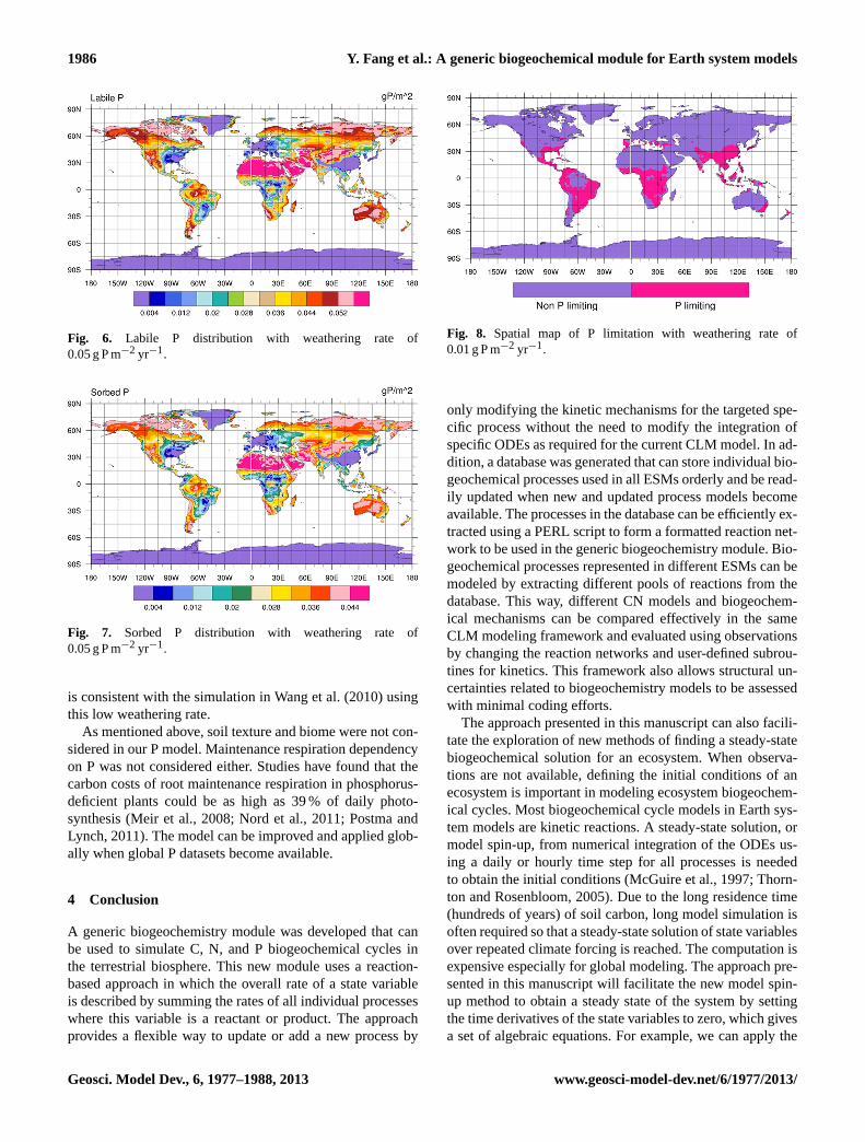
With the P weathering rate of 0.05 g P m−2 yr−1, almostno P limiting on productivity was shown. Figures 6 and 7show the distribution of labile and sorbed P after two yearsof simulated time. Total labile and sorbed P account for 18 %and 14 % of total P in soil, respectively.

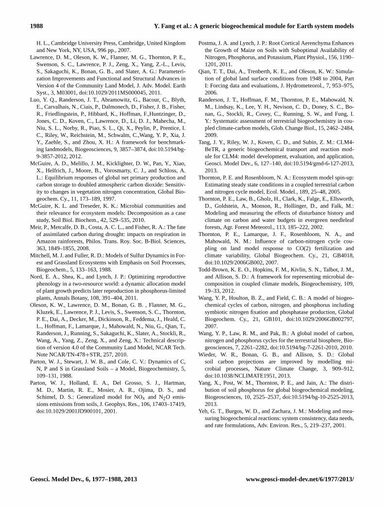
When the weathering rate is decreased to0.01 g P m−2 yr−1, Fig. 8 shows the P-limited regions.P limiting on NPP of tropical evergreen forest and savannah

www.geosci-model-dev.net/6/1977/2013/ Geosci. Model Dev., 6, 1977–1988, 2013

1986 Y. Fang et al.: A generic biogeochemical module for Earth system models

Fig. 6. Labile P distribution with weathering rate of0.05 g P m−2 yr−1.

Fig. 7. Sorbed P distribution with weathering rate of0.05 g P m−2 yr−1.

is consistent with the simulation in Wang et al. (2010) usingthis low weathering rate.

As mentioned above, soil texture and biome were not con-sidered in our P model. Maintenance respiration dependencyon P was not considered either. Studies have found that thecarbon costs of root maintenance respiration in phosphorus-deficient plants could be as high as 39 % of daily photo-synthesis (Meir et al., 2008; Nord et al., 2011; Postma andLynch, 2011). The model can be improved and applied glob-ally when global P datasets become available.

4 Conclusion

A generic biogeochemistry module was developed that canbe used to simulate C, N, and P biogeochemical cycles inthe terrestrial biosphere. This new module uses a reaction-based approach in which the overall rate of a state variableis described by summing the rates of all individual processeswhere this variable is a reactant or product. The approachprovides a flexible way to update or add a new process by

Fig. 8. Spatial map of P limitation with weathering rate of0.01 g P m−2 yr−1.

only modifying the kinetic mechanisms for the targeted spe-cific process without the need to modify the integration ofspecific ODEs as required for the current CLM model. In ad-dition, a database was generated that can store individual bio-geochemical processes used in all ESMs orderly and be read-ily updated when new and updated process models becomeavailable. The processes in the database can be efficiently ex-tracted using a PERL script to form a formatted reaction net-work to be used in the generic biogeochemistry module. Bio-geochemical processes represented in different ESMs can bemodeled by extracting different pools of reactions from thedatabase. This way, different CN models and biogeochem-ical mechanisms can be compared effectively in the sameCLM modeling framework and evaluated using observationsby changing the reaction networks and user-defined subrou-tines for kinetics. This framework also allows structural un-certainties related to biogeochemistry models to be assessedwith minimal coding efforts.

The approach presented in this manuscript can also facili-tate the exploration of new methods of finding a steady-statebiogeochemical solution for an ecosystem. When observa-tions are not available, defining the initial conditions of anecosystem is important in modeling ecosystem biogeochem-ical cycles. Most biogeochemical cycle models in Earth sys-tem models are kinetic reactions. A steady-state solution, ormodel spin-up, from numerical integration of the ODEs us-ing a daily or hourly time step for all processes is neededto obtain the initial conditions (McGuire et al., 1997; Thorn-ton and Rosenbloom, 2005). Due to the long residence time(hundreds of years) of soil carbon, long model simulation isoften required so that a steady-state solution of state variablesover repeated climate forcing is reached. The computation isexpensive especially for global modeling. The approach pre-sented in this manuscript will facilitate the new model spin-up method to obtain a steady state of the system by settingthe time derivatives of the state variables to zero, which givesa set of algebraic equations. For example, we can apply the

Geosci. Model Dev., 6, 1977–1988, 2013 www.geosci-model-dev.net/6/1977/2013/

Y. Fang et al.: A generic biogeochemical module for Earth system models 1987

Newton–Raphson method to the algebraic equations to solvethe steady-state solution. This is especially useful when thedecomposition of carbon pools is represented by nonlinearkinetics.

The approach represents a cost-effective way for the CLMcommunity to model biogeochemical processes and providesan efficient way to integrate new and updated process mod-els. In addition, the reaction database approach provides amutually understandable venue to communicate with biogeo-chemists for improvement of model process representationsand even inspire new research.

5 Code availability

The source code of the generic algorithm and PERL scriptcan be obtained upon request. Contact: yilin.fang@pnnl.gov.

Appendix A

Table A1. List of abbreviations.

acwd N : C (gN g−1C) ratio in coarse woody debris poolalitr1 N : C (gN g−1C) ratio in litter pool 1alitr2 N : C (gN g−1C) ratio in litter pool 2alitr3 N : C (gN g−1C) ratio in litter pool 3asoil1 N : C (gN g−1C) ratio in soil organic matter pool 1asoil2 N : C (gN g−1C) ratio in soil organic matter pool 2asoil3 N : C (gN g−1C) ratio in soil organic matter pool 3asoil4 N : C (gN g−1C) ratio in soil organic matter pool 4blitr1 P: C (gP g−1C) ratio in litter pool 1bsoil1 P: C (gP g−1C) ratio in soil organic matter pool 1Ccwd carbon in coarse woody debris poolClitr1 carbon in litter pool 1Clitr2 carbon in litter pool 2Clitr3 carbon in litter pool 3Csoil1 carbon in soil organic matter pool 1Csoil2 carbon in soil organic matter pool 2Csoil3 carbon in soil organic matter pool 3Csoil4 carbon in soil organic matter pool 4Ncwd nitrogen in coarse woody debris poolNlitr1 nitrogen in litter pool 1Nlitr2 nitrogen in litter pool 2Nlitr3 nitrogen in litter pool 3Nsoil1 nitrogen in soil organic matter pool 1Nsoil2 nitrogen in soil organic matter pool 2Nsoil3 nitrogen in soil organic matter pool 3Nsoil4 nitrogen in soil organic matter pool 4Nsmin mineral nitrogen in soilPlitr1 phosphorus in litter pool 1Plabile phosphorus in the labile soil poolPsoil1 phosphorus in soil organic matter pool 1Psoil2 phosphorus in soil organic matter pool 2Psoil3 phosphorus in soil organic matter pool 3Psorbed sorbed phosphorus pool in soilPssorbed strongly sorbed phosphorus pool in soilPoccluded occluded phosphorus pool in soil

Supplementary material related to this article isavailable online athttp://www.geosci-model-dev.net/6/1977/2013/gmd-6-1977-2013-supplement.zip.

Acknowledgements.This research has been accomplished throughfunding support from Pacific Northwest National Laboratory’sLaboratory Directed Research and Development Program. Aportion of this research was performed using PNNL InstitutionalComputing at Pacific Northwest National Laboratory. PNNL isoperated by Battelle for the US Department of Energy underContract DE-AC05-76RL01830.

Edited by: D. Lunt

References

Aguilera, D. R., Jourabchi, P., Spiteri, C., and Regnier, P.: Aknowledge-based reactive transport approach for the simulationof biogeochemical dynamics in Earth systems, Geochem. Geo-phys. Geosyst., 6, Q07012, doi:10.1029/2004GC000899, 2005.

Allison, S. D. and Martiny, J. B. H.: Resistance, resilience, and re-dundancy in microbial communities, Proc. Natl. Aca. Sci. USA,105, 11512–11519, 2008.

Bradford, M. A., Davies, C. A., Frey, S. D., Maddox, T. R.,Melillo, J. M., Mohan, J. E., Reynolds, J. F., Treseder, K. K.,and Wallenstein, M. D.: Thermal adaptation of soil microbialrespirationto elevated temperature, Ecol. Lett., 11, 1316–1327,doi:10.1111/j.1461-0248.2008.01251.x, 2008.

Buendía, C., Kleidon, A., and Porporato, A.: The role of tectonicuplift, climate, and vegetation in the long-term terrestrial phos-phorous cycle, Biogeosciences, 7, 2025–2038, doi:10.5194/bg-7-2025-2010, 2010.

Bünemann, E. K. and Condron, L. M.: Phosphorus and Sulphur Cy-cling in Terrestrial Ecosystems, in: Soil Biology, Nutrient Cy-cling in Terrestrial Ecosystems, edited by: Marschner, P. andRengel Z., Springer, New York, 65–92, 2007.

Chilakapati, A., Yabusaki, S., Szecsody, J., and MacEvoy, W.:Groundwater flow, multicomponent transport and biogeochem-istry: development and application of a coupled process model,J. Contaminant Hydrol., 43, 303–325, 2000.

Fang, Y., Yeh, G. T., and Burgos, W. D.: A generalparadigm to model reaction-based biogeochemical pro-cesses in batch systems, Water Resour. Res., 39, 1083,doi:10.1029/2002WR001694, 2003.

Goll, D. S., Brovkin, V., Parida, B. R., Reick, C. H., Kattge, J., Re-ich, P. B., van Bodegom, P. M., and Niinemets, Ü.: Nutrient lim-itation reduces land carbon uptake in simulations with a modelof combined carbon, nitrogen and phosphorus cycling, Biogeo-sciences, 9, 3547–3569, doi:10.5194/bg-9-3547-2012, 2012.

Gu, C., Laverman, A. M., and Pallud, C. E.: Environmental con-trols on nitrogen and sulfur cycles in surficial aquatic sediments,Front. Microbiol., 3, 45, doi:10.3389/fmicb.2012.00045, 2012.

IPCC: Contribution of Working Group I to the Fourth AssessmentReport of the Intergovernmental Panel on Climate Change: ThePhysical Science, edited by: Solomon, S., Qin, D., Manning, M.,Chen, Z., Marquis, M., Averyt, K. B., Tignor, M., and. Miller,

www.geosci-model-dev.net/6/1977/2013/ Geosci. Model Dev., 6, 1977–1988, 2013

1988 Y. Fang et al.: A generic biogeochemical module for Earth system models

H. L., Cambridge University Press, Cambridge, United Kingdomand New York, NY, USA, 996 pp., 2007.

Lawrence, D. M., Oleson, K. W., Flanner, M. G., Thornton, P. E.,Swenson, S. C., Lawrence, P. J., Zeng, X., Yang, Z.-L., Levis,S., Sakaguchi, K., Bonan, G. B., and Slater, A. G.: Parameteri-zation Improvements and Functional and Structural Advances inVersion 4 of the Community Land Model, J. Adv. Model. EarthSyst., 3, M03001, doi:10.1029/2011MS000045, 2011.

Luo, Y. Q., Randerson, J. T., Abramowitz, G., Bacour, C., Blyth,E., Carvalhais, N., Ciais, P., Dalmonech, D., Fisher, J. B., Fisher,R., Friedlingstein, P., Hibbard, K., Hoffman, F.,Huntzinger, D.,Jones, C. D., Koven, C., Lawrence, D., Li, D. J., Mahecha, M.,Niu, S. L., Norby, R., Piao, S. L., Qi, X., Peylin, P., Prentice, I.C., Riley, W., Reichstein, M., Schwalm, C.,Wang, Y. P., Xia, J.Y., Zaehle, S., and Zhou, X. H.: A framework for benchmark-ing landmodels, Biogeosciences, 9, 3857–3874, doi:10.5194/bg-9-3857-2012, 2012.

McGuire, A. D., Melillo, J. M., Kicklighter, D. W., Pan, Y., Xiao,X., Helfrich, J., Moore, B., Vorosmarty, C. J., and Schloss, A.L.: Equilibrium responses of global net primary production andcarbon storage to doubled atmospheric carbon dioxide: Sensitiv-ity to changes in vegetation nitrogen concentration, Global Bio-geochem. Cy., 11, 173–189, 1997.

McGuire, K. L. and Treseder, K. K.: Microbial communities andtheir relevance for ecosystem models: Decomposition as a casestudy, Soil Biol. Biochem., 42, 529–535, 2010.

Meir, P., Metcalfe, D. B., Costa, A. C. L., and Fisher, R. A.: The fateof assimilated carbon during drought: impacts on respiration inAmazon rainforests, Philos. Trans. Roy. Soc. B-Biol. Sciences,363, 1849–1855, 2008.

Mitchell, M. J. and Fuller, R. D.: Models of Sulfur Dynamics in For-est and Grassland Ecosystems with Emphasis on Soil Processes,Biogeochem., 5, 133–163, 1988.

Nord, E. A., Shea, K., and Lynch, J. P.: Optimizing reproductivephenology in a two-resource world: a dynamic allocation modelof plant growth predicts later reproduction in phosphorus-limitedplants, Annals Botany, 108, 391–404, 2011.

Oleson, K. W., Lawrence, D. M., Bonan, G. B. , Flanner, M. G.,Kluzek, E., Lawrence, P. J., Levis, S., Swenson, S. C., Thornton,P. E., Dai, A., Decker, M., Dickinson, R., Feddema, J., Heald, C.L., Hoffman, F., Lamarque, J., Mahowald, N., Niu, G., Qian, T.,Randerson, J., Running, S., Sakaguchi, K., Slater, A., Stockli, R.,Wang, A., Yang, Z., Zeng, X., and Zeng, X.: Technical descrip-tion of version 4.0 of the Community Land Model, NCAR Tech.Note NCAR/TN-478+STR, 257, 2010.

Parton, W. J., Stewart, J. W. B., and Cole, C. V.: Dynamics of C,N, P and S in Grassland Soils – a Model, Biogeochemistry, 5,109–131, 1988.

Parton, W. J., Holland, E. A., Del Grosso, S. J., Hartman,M. D., Martin, R. E., Mosier, A. R., Ojima, D. S., andSchimel, D. S.: Generalized model for NOx and N2O emis-sions emissions from soils, J. Geophys. Res., 106, 17403–17419,doi:10.1029/2001JD900101, 2001.

Postma, J. A. and Lynch, J. P.: Root Cortical Aerenchyma Enhancesthe Growth of Maize on Soils with Suboptimal Availability ofNitrogen, Phosphorus, and Potassium, Plant Physiol., 156, 1190–1201, 2011.

Qian, T. T., Dai, A., Trenberth, K. E., and Oleson, K. W.: Simula-tion of global land surface conditions from 1948 to 2004, PartI: Forcing data and evaluations, J. Hydrometeorol., 7, 953–975,2006.

Randerson, J. T., Hoffman, F. M., Thornton, P. E., Mahowald, N.M., Lindsay, K., Lee, Y. H., Nevison, C. D., Doney, S. C., Bo-nan, G., Stockli, R., Covey, C., Running, S. W., and Fung, I.Y.: Systematic assessment of terrestrial biogeochemistry in cou-pled climate-carbon models, Glob. Change Biol., 15, 2462–2484,2009.

Tang, J. Y., Riley, W. J., Koven, C. D., and Subin, Z. M.: CLM4-BeTR, a generic biogeochemical transport and reaction mod-ule for CLM4: model development, evaluation, and application,Geosci. Model Dev., 6, 127–140, doi:10.5194/gmd-6-127-2013,2013.

Thornton, P. E. and Rosenbloom, N. A.: Ecosystem model spin-up:Estimating steady state conditions in a coupled terrestrial carbonand nitrogen cycle model, Ecol. Model., 189, 25–48, 2005.

Thornton, P. E., Law, B., Gholz, H., Clark, K., Falge, E., Ellsworth,D., Goldstein, A., Monson, R., Hollinger, D., and Falk, M.:Modeling and measuring the effects of disturbance history andclimate on carbon and water budgets in evergreen needleleafforests, Agr. Forest Meteorol., 113, 185–222, 2002.

Thornton, P. E., Lamarque, J. F., Rosenbloom, N. A., andMahowald, N. M.: Influence of carbon-nitrogen cycle cou-pling on land model response to CO(2) fertilization andclimate variability, Global Biogeochem. Cy., 21, GB4018,doi:10.1029/2006GB002, 2007.

Todd-Brown, K. E. O., Hopkins, F. M., Kivlin, S. N., Talbot, J. M.,and Allison, S. D.: A framework for representing microbial de-composition in coupled climate models, Biogeochemistry, 109,19–33, 2012.

Wang, Y. P., Houlton, B. Z., and Field, C. B.: A model of biogeo-chemical cycles of carbon, nitrogen, and phosphorus includingsymbiotic nitrogen fixation and phosphatase production, GlobalBiogeochem. Cy., 21, GB101, doi:10.1029/2006GB002797,2007.

Wang, Y. P., Law, R. M., and Pak, B.: A global model of carbon,nitrogen and phosphorus cycles for the terrestrial biosphere, Bio-geosciences, 7, 2261–2282, doi:10.5194/bg-7-2261-2010, 2010.

Wieder, W. R., Bonan, G. B., and Allison, S. D.: Globalsoil carbon projections are improved by modelling mi-crobial processes, Nature Climate Change, 3, 909–912,doi:10.1038/NCLIMATE1951, 2013.

Yang, X., Post, W. M., Thornton, P. E., and Jain, A.: The distri-bution of soil phosphorus for global biogeochemical modeling,Biogeosciences, 10, 2525–2537, doi:10.5194/bg-10-2525-2013,2013.

Yeh, G. T., Burgos, W. D., and Zachara, J. M.: Modeling and mea-suring biogeochemical reactions: system consistency, data needs,and rate formulations, Adv. Environ. Res., 5, 219–237, 2001.

Geosci. Model Dev., 6, 1977–1988, 2013 www.geosci-model-dev.net/6/1977/2013/