a genetic algorithm for period vehicle routing problem with practical application josÉ lassance de...
TRANSCRIPT
A GENETIC ALGORITHM FOR PERIOD VEHICLE ROUTING PROBLEM WITH PRACTICAL
APPLICATION
JOSÉ LASSANCE DE CASTRO SILVA
FELIPE PINHEIRO BEZERRA
CYTEDHAROSA 20121
UNIVERSIDADE FEDERAL DO CEARÁ
PRÓ-REITORIA DE PESQUISA E PÓS-GRADUAÇÃO
PROGRAMA DE MESTRADO EM LOGÍSTICA E PESQUISA OPERACIONAL
Outline
Motivating Problem Problem Definition Solution Method Aproach Computational Experiments Conclusions and Future Research Directions
Motivating Problem
Practical application:
Wholesaler Distributor
Ice cream and ice pops division
Sales team
Marketing mix:
Product
Pricing
Promotion
Placement3

Motivating Problem
Practical application:
SALES TEAM ROUTINE AT CUSTOMER STORE
• Observe visibility and promotion elements
• Inspect equipments (freezers)
• Clean the equipments and rearrange the products inside them
• Remove strange products
• Analyse supply, assortment and prices
• Negotiate improvements and orders
• Place order
4
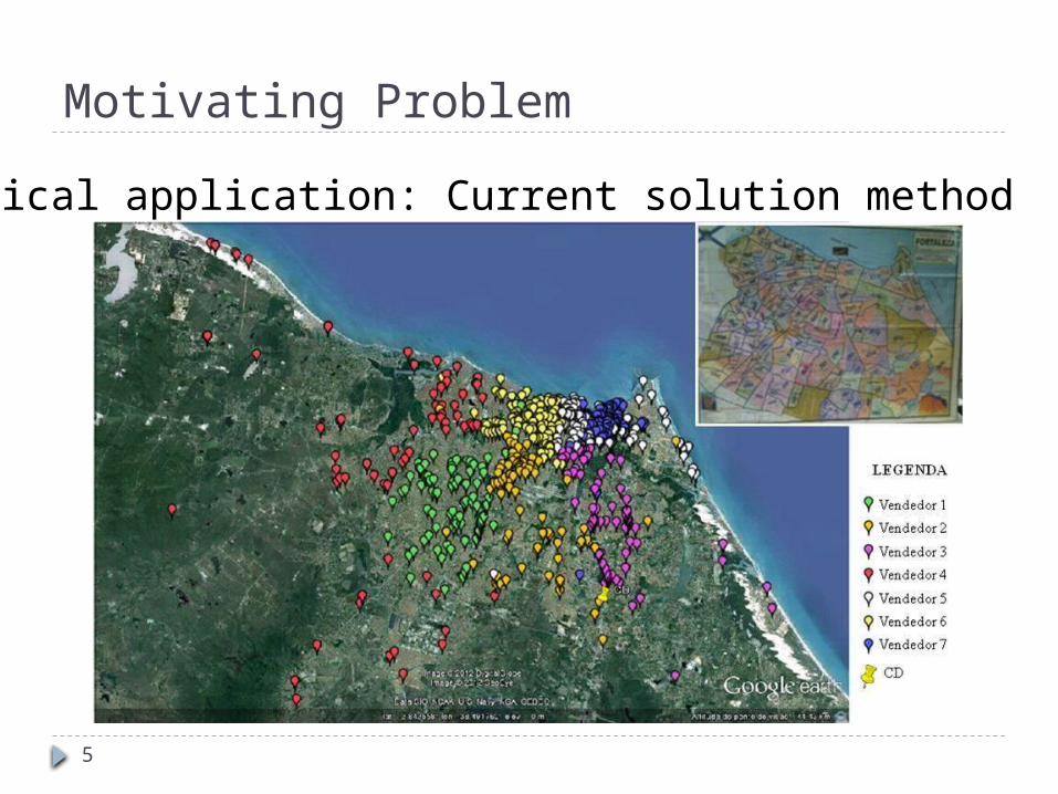
Motivating Problem
Practical application: Current solution method
5

Motivating Problem
Practical application: Current solution method
Advantages:
Out of route serving
Intuitive inclusion of new customers
Sales representative´s familiarity with territory
6
Motivating Problem
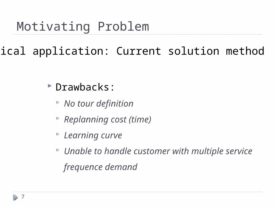
Practical application: Current solution method
Drawbacks:
No tour definition
Replanning cost (time)
Learning curve
Unable to handle customer with multiple service
frequence demand
7
Motivating Problem
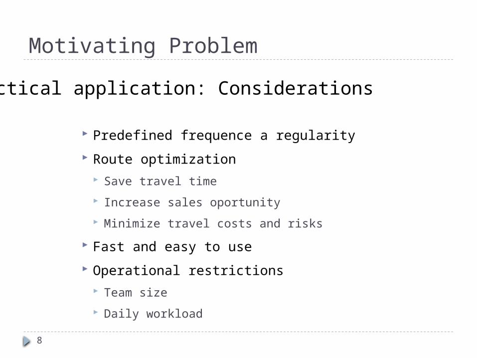
Practical application: Considerations
Predefined frequence a regularity
Route optimization
Save travel time
Increase sales oportunity
Minimize travel costs and risks
Fast and easy to use
Operational restrictions
Team size
Daily workload8
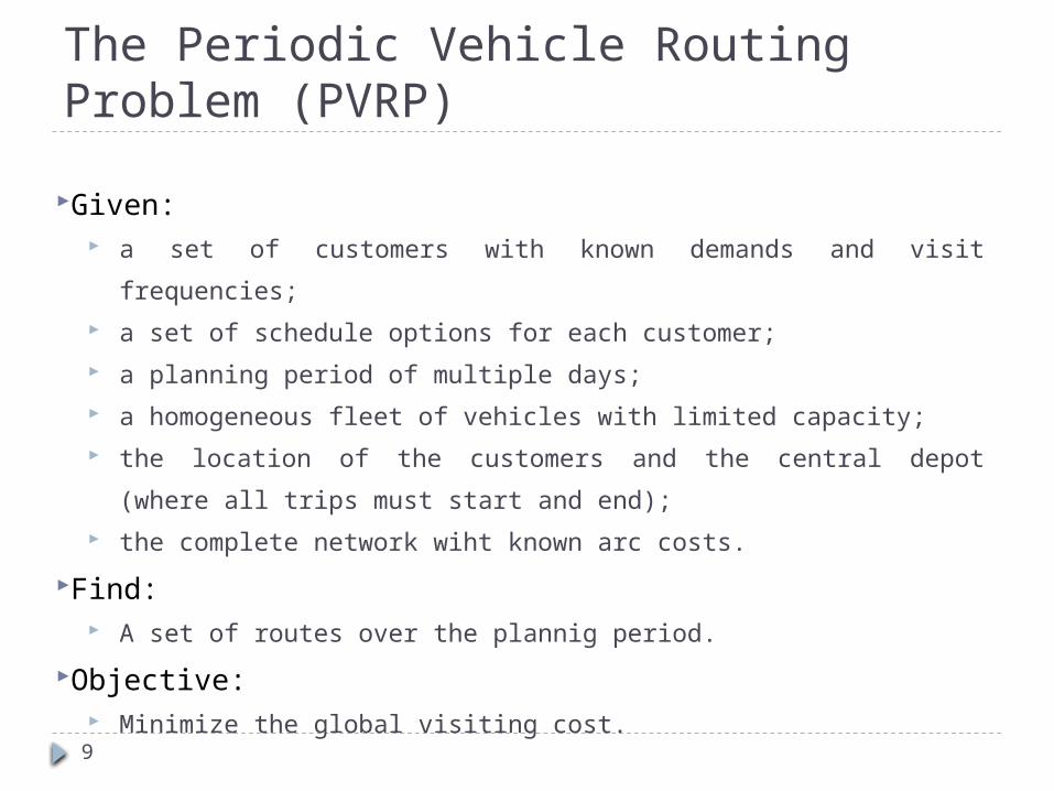
The Periodic Vehicle Routing Problem (PVRP)
Given: a set of customers with known demands and visit frequencies;
a set of schedule options for each customer;
a planning period of multiple days;
a homogeneous fleet of vehicles with limited capacity;
the location of the customers and the central depot (where all trips must start and end);
the complete network wiht known arc costs.
Find: A set of routes over the plannig period.
Objective: Minimize the global visiting cost.
9
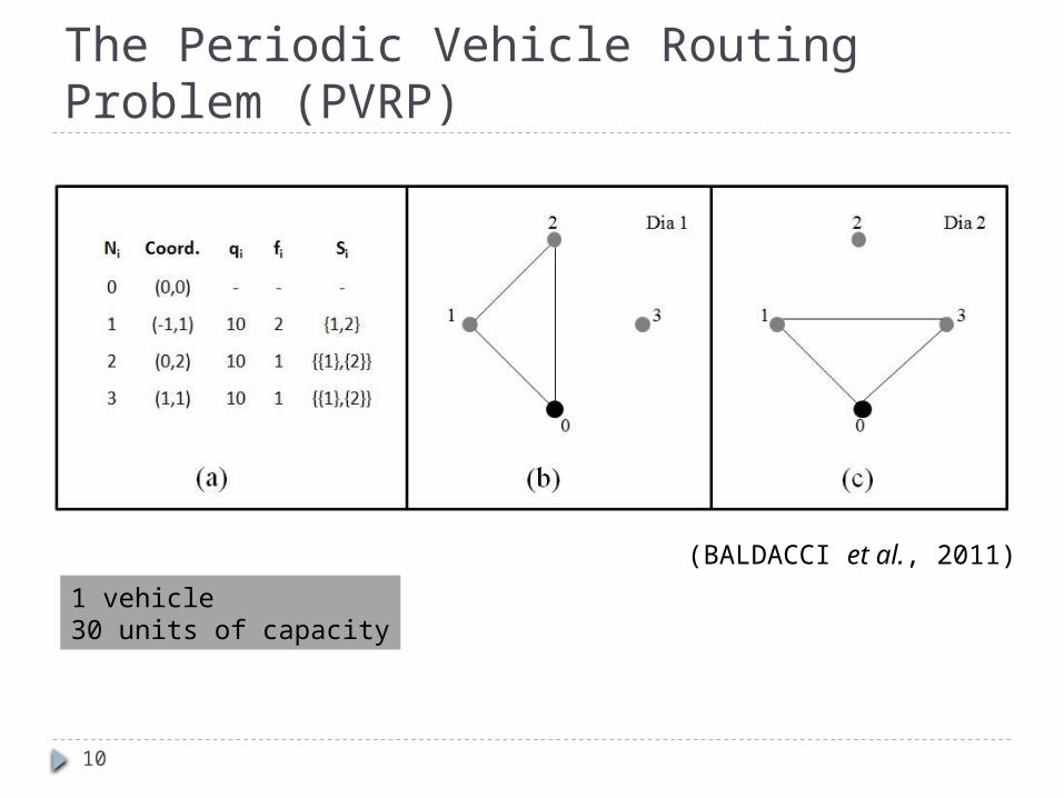
The Periodic Vehicle Routing Problem (PVRP)
(BALDACCI et al., 2011)
10
1 vehicle30 units of capacity

Select a visit schedule for each customer;
Define the customers that should be visited by each
vehicle on each day;
Route the vehicles for each day.
Three simultaneous decisions:
11
The Periodic Vehicle Routing Problem (PVRP)
It´s a generalization of the VRP: NP-Hard.

Solution Method Aproach
Genetic Algorithms: Concepts
Holland (1975)
Metaheuristic
Natural selection
Population based
Cromossomes/individuals
Recombinations
Fitness12
Solution Method Aproach
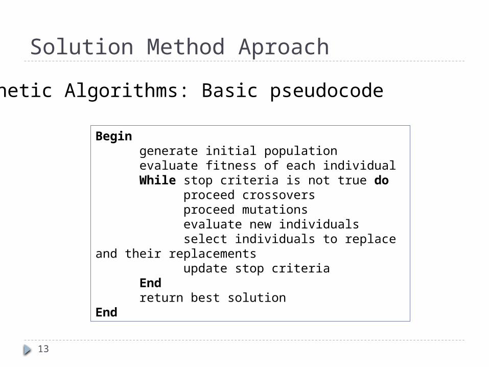
Genetic Algorithms: Basic pseudocode
Begin generate initial population evaluate fitness of each individual While stop criteria is not true do proceed crossovers proceed mutations evaluate new individuals select individuals to replace and their replacements update stop criteria End return best solutionEnd
13

Solution Method Aproach
Genetic Algorithms: Key points
Solution representation
Fitness function
Population control
Selection method
Genetic operators
Use of hibridization
Stop criteria
Parameters definition14

Solution Method Aproach
Proposed genetic algorithm:
Solution representation
Grand Tour
No trip delimiters
Prins (2004), Chu et al. (2004) e Vidal et al. (2012)
(VIDAL et al. 2012)15
Solution Method Aproach
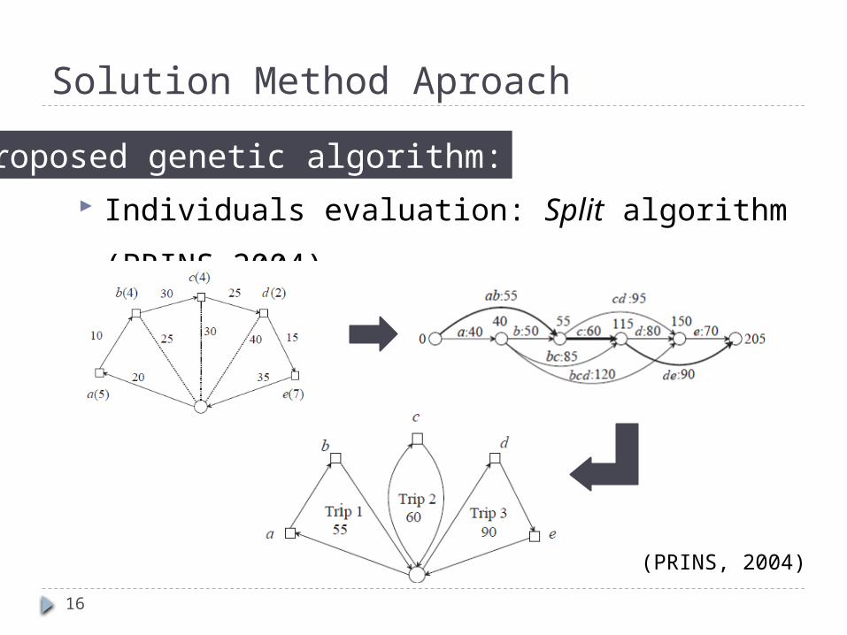
Proposed genetic algorithm:
Individuals evaluation: Split algorithm (PRINS 2004)
(PRINS, 2004)
16
Solution Method Aproach
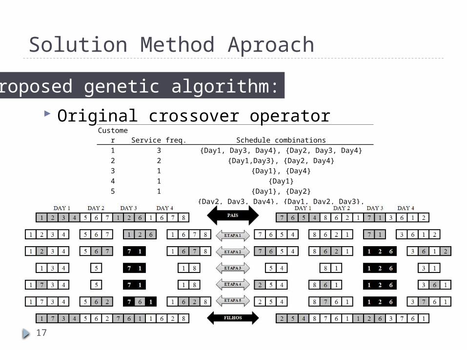
Proposed genetic algorithm:
Original crossover operatorCustomer Service freq. Schedule combinations
1 3 {Day1, Day3, Day4}, {Day2, Day3, Day4}2 2 {Day1,Day3}, {Day2, Day4}3 1 {Day1}, {Day4}4 1 {Day1}5 1 {Day1}, {Day2}6 3 {Day2, Day3, Day4}, {Day1, Day2, Day3}, {Day1, Day2, Day4}7 2 {Day1,Day3}, {Day2, Day4}8 1 {Day2}, {Day3}
17
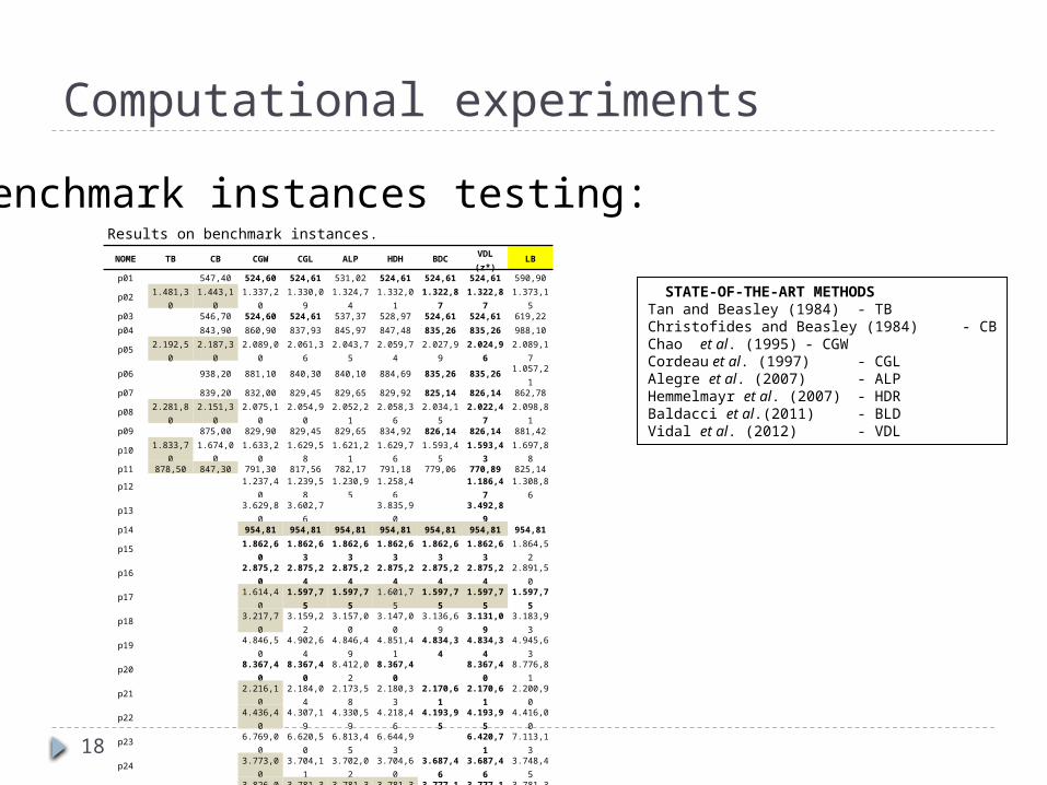
Computational experiments
Benchmark instances testing:NOME TB CB CGW CGL ALP HDH BDC VDL (z*) LB
p01 547,40 524,60 524,61 531,02 524,61 524,61 524,61 590,90
p02 1.481,30 1.443,10 1.337,20 1.330,09 1.324,74 1.332,01 1.322,87 1.322,87 1.373,15
p03 546,70 524,60 524,61 537,37 528,97 524,61 524,61 619,22
p04 843,90 860,90 837,93 845,97 847,48 835,26 835,26 988,10
p05 2.192,50 2.187,30 2.089,00 2.061,36 2.043,75 2.059,74 2.027,99 2.024,96 2.089,17
p06 938,20 881,10 840,30 840,10 884,69 835,26 835,26 1.057,21
p07 839,20 832,00 829,45 829,65 829,92 825,14 826,14 862,78
p08 2.281,80 2.151,30 2.075,10 2.054,90 2.052,21 2.058,36 2.034,15 2.022,47 2.098,81
p09 875,00 829,90 829,45 829,65 834,92 826,14 826,14 881,42
p10 1.833,70 1.674,00 1.633,20 1.629,58 1.621,21 1.629,76 1.593,45 1.593,43 1.697,88p11 878,50 847,30 791,30 817,56 782,17 791,18 779,06 770,89 825,14
p12 1.237,40 1.239,58 1.230,95 1.258,46 1.186,47 1.308,86
p13 3.629,80 3.602,76 3.835,90 3.492,89
p14 954,81 954,81 954,81 954,81 954,81 954,81 954,81
p15 1.862,60 1.862,63 1.862,63 1.862,63 1.862,63 1.862,63 1.864,52
p16 2.875,20 2.875,24 2.875,24 2.875,24 2.875,24 2.875,24 2.891,50
p17 1.614,40 1.597,75 1.597,75 1.601,75 1.597,75 1.597,75 1.597,75
p18 3.217,70 3.159,22 3.157,00 3.147,00 3.136,69 3.131,09 3.183,93
p19 4.846,50 4.902,64 4.846,49 4.851,41 4.834,34 4.834,34 4.945,63
p20 8.367,40 8.367,40 8.412,02 8.367,40 8.367,40 8.776,81
p21 2.216,10 2.184,04 2.173,58 2.180,33 2.170,61 2.170,61 2.200,90
p22 4.436,40 4.307,19 4.330,59 4.218,46 4.193,95 4.193,95 4.416,00
p23 6.769,00 6.620,50 6.813,45 6.644,93 6.420,71 7.113,13
p24 3.773,00 3.704,11 3.702,02 3.704,60 3.687,46 3.687,46 3.748,45
p25 3.826,00 3.781,38 3.781,38 3.781,38 3.777,15 3.777,15 3.781,38
p26 3.834,00 3.795,32 3.795,33 3.795,32 3.795,32 3.795,32 3.810,61
p27 23.401,60 23.017,45 22.561,33 22.153,31 21.912,85 21.833,87 22.378,36
p28 23.105,10 22.569,40 22.562,44 22.418,52 22.242,51 22.242,51 22.693,78
p29 24.248,20 24.012,92 23.752,15 22.864,23 22.543,76 22.543,75 23.021,93
p30 80.982,10 77.179,33 76.793,99 75.579,23 74.464,26 73.875,19 76.639,43
p31 80.279,10 79.382,35 77.944,79 77.459,14 76.322,04 76.001,57 78.309,61
p32 83.838,70 80.908,95 81.055,52 79.487,97 78.072,88 77.598,00 80.756,82
DESVIO 12,4% 6,2% 2,9% 1,8% 1,6% 1,6% 0,1% 0,0% 5,4%
STATE-OF-THE-ART METHODSTan and Beasley (1984) - TBChristofides and Beasley (1984) - CBChao et al. (1995) - CGWCordeau et al. (1997) - CGLAlegre et al. (2007) - ALPHemmelmayr et al. (2007) - HDRBaldacci et al.(2011) - BLDVidal et al. (2012) - VDL
Results on benchmark instances.
18
Computational experiments
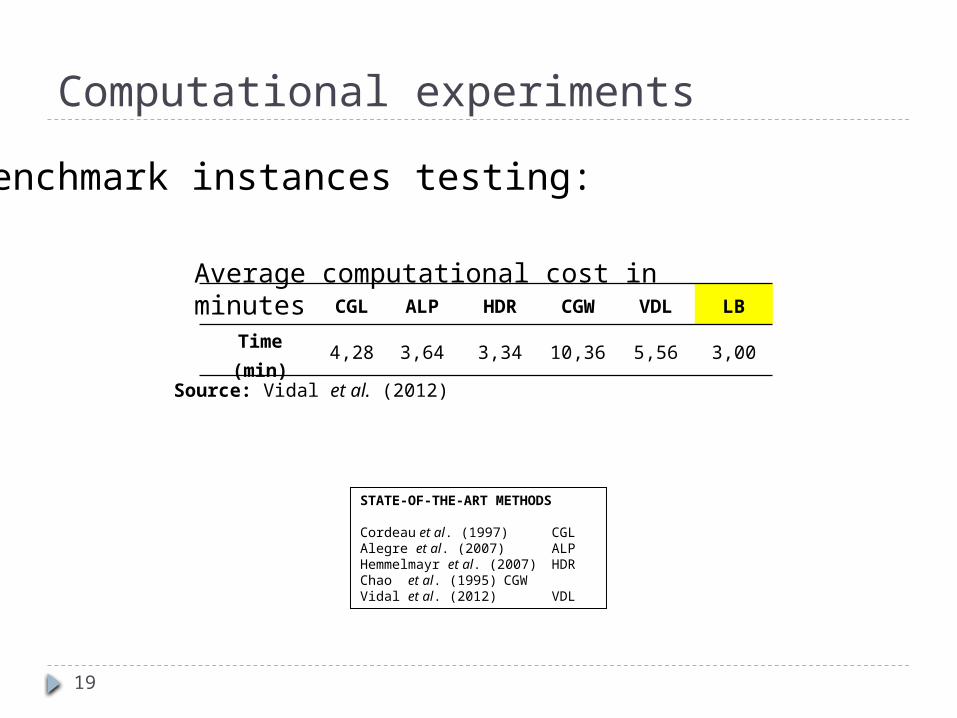
Benchmark instances testing:
CGL ALP HDR CGW VDL LB
Time (min) 4,28 3,64 3,34 10,36 5,56 3,00
STATE-OF-THE-ART METHODS
Cordeau et al. (1997) CGLAlegre et al. (2007) ALPHemmelmayr et al. (2007) HDRChao et al. (1995) CGWVidal et al. (2012) VDL
Source: Vidal et al. (2012)
Average computational cost in minutes
19

Computational experiments
Benchmark instances testing:
Fair results
Low computational costs
20

Computational experiments
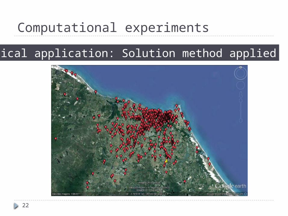
Practical application: Solution method applied
Briefing
629 Stores
7 sales representatives
Weekly visits, from monday through friday
5 schedule options, except for 36 customers
Service time: 15 minutes
Maximum daily workload: 8 hours (480 minutes)
Travel speed: 30km/h
21
Computational experiments
Practical application: Solution method applied
22

Computational experiments
Practical application: Solution method applied
Adjustments:
Demand = service time
Restrictions = daily workload in mimutes
Travel time
Penalties for not using every “vehicle” daily
23

Computational experiments
Practical application: Solution method applied
Current method
Proposed method A
Proposed method B
Daily workload considered (min) 480,00 480,00 425,00
Total distance (km) 1.337,40 956,80 1.188,84
Savings (km) - 380,60 148,56
Savings (%) - 28,46 11,11
Current method
Proposed method A
Proposed method B
Daily workload considered 480,00 480,00 425,00
Daily workload proposed 346,00 324,25 337,51
Total service time 269,57 269,57 269,57
Total travel time 76,42 54,67 67,93
Total downtime 134,00 155,75 142,49
Minimum daily workload 195,46 15,39 35,65
Maximum daily workload 550,28 464,42 409,86
Standart deviation 75,41 167,49 87,02
Distance savings over planning period
Average daily workload composition per salesman (minutes).
24

Computational experiments
Practical application: Solution method applied
Initial findings:
Downtime awareness
Trade-off between savings and workload balancing
“How much does the workload balancing cost?”
25
Computational experiments
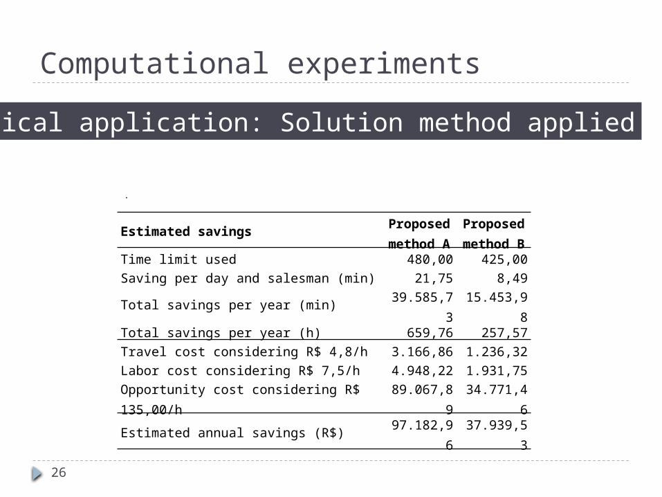
Practical application: Solution method applied
Estimated savingsProposed method A
Proposed method B
Time limit used 480,00 425,00
Saving per day and salesman (min) 21,75 8,49
Total savings per year (min) 39.585,73 15.453,98
Total savings per year (h) 659,76 257,57
Travel cost considering R$ 4,8/h 3.166,86 1.236,32
Labor cost considering R$ 7,5/h 4.948,22 1.931,75
Opportunity cost considering R$ 135,00/h 89.067,89 34.771,46
Estimated annual savings (R$) 97.182,96 37.939,53
.
26

Computational experiments
Practical application: Solution method applied
Current method Proposed method Savings
Week dayDistance
(Km)Workload
(Min)Distance
(Km)Workload
(Min)Distance Workload
monday 252,55 2.545,11 228,51 2.197,03 10% 14%
tuesday 246,03 2.427,06 221,08 2.542,16 10% -5%
wednesday 284,17 2.323,34 235,75 2.256,50 17% 3%
thursday 277,66 2.445,33 254,90 2.384,80 8% 2%
friday 277,02 2.369,04 248,59 2.432,19 10% -3%
Total 1.337,44 12.109,87 1.188,84 11.812,68 11% 2%
Comparisons between current solution method and proposed solution method
27
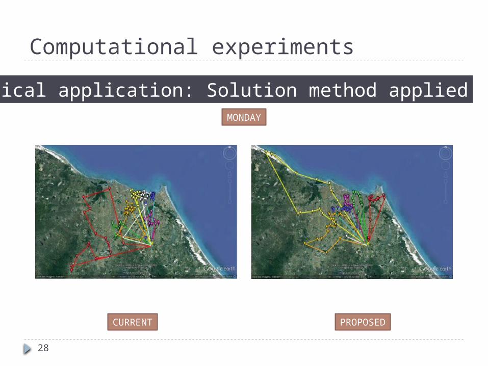
Computational experiments
Practical application: Solution method appliedMONDAY
CURRENT PROPOSED
28
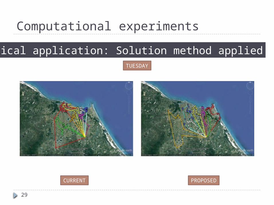
Computational experiments
Practical application: Solution method applied
29
TUESDAY
CURRENT PROPOSED
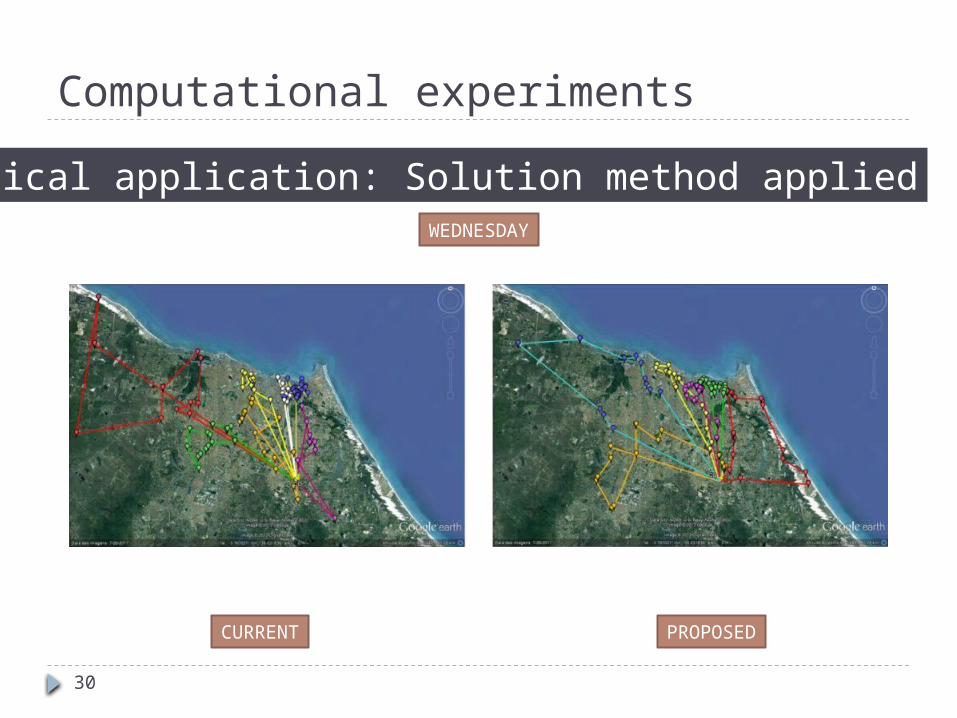
Computational experiments
Practical application: Solution method applied
30
WEDNESDAY
CURRENT PROPOSED

Computational experiments
Practical application: Solution method applied
31
THURSDAY
CURRENT PROPOSED

Computational experiments
Practical application: Solution method applied
32
FRIDAY
CURRENT PROPOSED
Conclusions
Good solution method for the PVRP
Good results for the practical case: Route optimization
Reliable procedure
Service level guaranteed
Cost control
Easy set-up
Decision making tool
33

Future Research Directions
Testing another insertion methods (i.e. GENI)
Population diversity control
Apply more mutation operators
Multicriteria analisys for fitness evaluation
Automatic and/or dynamic calibration
Meta-AGs
AI
34
Future Research Directions
Direct aproach for balancing
Spatial route clustering for each vehicle during
planning period
35

THANK YOU!
36
JOSÉ LASSANCE DE CASTRO SILVA <[email protected]>
FELIPE PINHEIRO BEZERRA <[email protected]>
CYTEDHAROSA 2012
UNIVERSIDADE FEDERAL DO CEARÁ
PRÓ-REITORIA DE PESQUISA E PÓS-GRADUAÇÃO
PROGRAMA DE MESTRADO EM LOGÍSTICA E PESQUISA OPERACIONAL