a gentle tutorial on statistical inversion using the...

A Gentle Tutorial on Statistical Inversion

using the Bayesian Paradigm

Tan Bui-Thanh∗

Institute for Computational Engineering and Sciences, The University of Texas at Austin

Contents

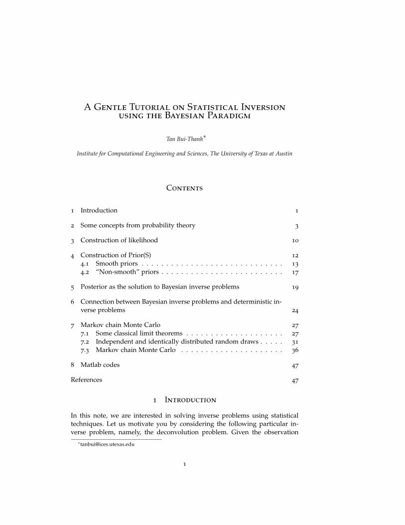
1 Introduction 1

2 Some concepts from probability theory 3

3 Construction of likelihood 10

4 Construction of Prior(S) 12

4.1 Smooth priors . . . . . . . . . . . . . . . . . . . . . . . . . . . . . 13

4.2 “Non-smooth” priors . . . . . . . . . . . . . . . . . . . . . . . . . 17

5 Posterior as the solution to Bayesian inverse problems 19

6 Connection between Bayesian inverse problems and deterministic in-verse problems 24

7 Markov chain Monte Carlo 27

7.1 Some classical limit theorems . . . . . . . . . . . . . . . . . . . . 27

7.2 Independent and identically distributed random draws . . . . . 31

7.3 Markov chain Monte Carlo . . . . . . . . . . . . . . . . . . . . . 36

8 Matlab codes 47

References 47

1 Introduction

In this note, we are interested in solving inverse problems using statisticaltechniques. Let us motivate you by considering the following particular in-verse problem, namely, the deconvolution problem. Given the observation∗[email protected]

1

mailto:[email protected]

1. Introduction

signal g(s), we would like to reconstruct the input signal f (t) : [0, 1] → R,where the observation and the input obey the following relation

(1) g(sj) =

1∫0

a(sj, t) f (t) dt, 0 ≤ j ≤ n.

Here, a : [0, 1] × [0, 1] → R is known as the blurring kernel. So, in fact wedon’t know the output signal completely, but at a finite number of observa-tion points. A straightforward approach you may think of is to apply somenumerical quadrature on the right side of (1), and then recover f (t) at thequadrature points by inverting the resulting matrix. If you do this, you realizethat the matrix is ill-conditioned, and it is not a good idea to invert it. Thereare techniques to go around this issue, but let us not pursue them here. In-stead, we recast the deconvolution task into an optimization problem such as

(2) minf (t)

n

∑j=0

g(sj)−1∫

0

a(sj, t) f (t) dt

2

.

However, the ill-conditioning nature of our inverse problem does not go away.Indeed, (2) may have multiple solutions and multiple minima. In addition, asolution to (2) may not depend continuously on g(sj), 0 ≤ j ≤ n. So what isthe point of recast? Clearly, if the cost function (also known as the data misfit)is a parabola, then the optimal solution is unique. This immediately suggeststhat one should add a quadratic term to the cost function to make it morelike a parabola, and hence making the optimization problem easier. This isessentially the idea behind the Tikhonov regularization, which proposes to solvethe nearby problem

minf (t)

n

∑j=0

g(sj)−1∫

0

a(sj, t) f (t) dt

2

+κ

2

∥∥∥R1/2 f∥∥∥2

,

where κ is known as the regularization parameter, and ‖·‖ is some appropriatenorm. Perhaps, two popular choices for R1/2 are ∇ and ∆, the gradient andLaplace operator, respectively, and we discuss them in details in the following.

Now, in practice, we are typically not able to observe g(sj) directly but itsnoise-corrupted value

gobs(sj) = g(sj) + ej, 0 ≤ j ≤ n,

where ej, j = 0, . . . , n, are some random noise. You can think of the noise asthe inaccuracy in observation/measurement devices. The question you may

2

2. Some concepts from probability theory

ask is how to incorporate this kind of randomness in the above deterministicsolution methods. There are works in this direction, but let us introduce astatistical framework based on the Bayesian paradigm to you in this note.This approach is appealing since it can incorporate most, if not all, kinds ofrandomness in a systematic manner.

A large portion of this note follows closely the presentation of two excellentbooks by Somersalo et al. [1, 2]. The pace is necessary slow since we developthis note for readers with minimal knowledge in probability theory. The onlyrequirement is to either be familiar with or adopt the conditional probabilityformula concept. This is the corner stone on which we build the rest of thetheory. Clearly, the theory we present here is by no means complete since thesubject is vast, and still under development.

Our presentation is in the form of dialogue, which we hope it is easierfor the readers to follow. We shall give a lot of little exercises along the wayto help understand the subject better. We also leave a large number of sidenotes, mostly in term of little questions, to keep the readers awake and makeconnections of different parts of the notes. On the other hand, we often dis-cuss deeper probability concepts in the footnotes to serve as starting pointsfor those who want to dive into the rigorous probability theory. Finally, wesupply Matlab codes at the end of the note so that the readers can use themto reproduce most of the results and to start their journey into the wonderfulworld of Bayesian inversion.

2 Some concepts from probability theory

We begin with the definition of randomness.

2.1 definition. An even is deterministic if its outcome is completely predictable.

2.2 definition. A random event is the complement of a deterministic event,that is, its outcome is not fully predictable.

2.3 example. If today is Wednesday, then “tomorrow is Thursday” is deter-ministic, but whether it rains tomorrow is not fully predictable.

As a result, randomness means lack of information and it is the directconsequence of our ignorance. To express our belief1 on random events, weuse probability; probability of uncertain events is always less than 1, an eventthat surely happens has probability 1, and an event that never happens has0 probability. In particular, to reflect the subjective nature, we call it subjective

1Different person has different belief which leads to different solution of the Bayesian inferenceproblem. Specifically, one’s belief is based on his known information (expressed in terms of σ-algebra) and “weights” on each information (expressed in terms of probability measure). That is,people working with different probability spaces have different solutions.

3


probability or Bayesian probability since it represents belief, and hence depend-ing upon one’s experience/knowledge to decide what is reasonable to believe.

2.4 example. Let us consider the event of tossing a coin. Clearly, this is arandom event since we don’t know whether head or tail will appear. Nev-ertheless, we believe that out of n tossing times, n/2 times is head and n/2times is tail.2 We express this belief in terms of probability as: the (subjective)probability of getting a head is 1

2 and the (subjective) probability of getting atail is 1

2 .

We define (Ω,F , P) as a probability space. One typically call Ω the samplespace, F a σ-algebra containing all events A ⊂ Ω, and P a probability measuredefined on F . We can think of an event A as information and the probabilitythat A happens, i.e. P [A], is the weight assigned to that information. Werequire that

0 ≤ P [A]def=∫A

dω ≤ 1, P [∅] = 0, P [Ω] = 1.

2.5 example. Back to the tossing coin example, we trivially have Ω = head, tail,F = ∅, head , tail , Ω. The weights are P [∅] = 0, P [tail] = P [head] =12 , and P [head, tail] = 1.

Two events A and B are independent3 if

P [A ∩ B] = P [A]×P [B] .

One of the central ideas in Bayesian probability is the conditional probabil-ity4. The conditional probability of A on/given B is defined as5

(3) P [A|B] = P[A∩B]P[B] ,

which can also be rephrased as the probability that A happens provided B hasThis is the corner stone formula to buildmost of results in this note, make sure thatyou feel comfortable with it. already happened.

2.6 example. Assume that we want to roll a dice. Denote B as the event ofgetting of face bigger than 4, and A the event of getting face 6. Using (3) we

2One can believe that out of n tossing times, n/3 times is head and 2n/3 times is tail if he usesan unfair coin.

3Probability theory is often believed to be a part of measure theory, but independence is whereit departs from the measure theory umbrella.

4A more general and rigorous tool is conditional expectation, a particular of which is condi-tional probability.

5This was initially introduced by Kolmogorov, a father of modern probability theory.

4


have

P [A|B] = 1/61/3

= 1/2.

We can solve the problem using a more elementary argument. B happenswhen we either get face 5 or face 6. The probability of getting face 6 when Bhas already happened is clearly 1

2 .

The conditional probability can also be understood as the probability whenthe sample space is restricted to B.

2.7 exercise. Determine P [A|B] in Figure 1.

Ω

B

A

(a) P [A|B] =

Ω

B

A

(b) P [A|B] =

Figure 1: Demonstration of conditional probability.

2.8 exercise. Show that the following Bayes formula for conditional probabil-ity holds

(4) P [A|B] = P[B|A]P[A]P[B] .

By inspection, if A and B are mutually independent, we have

P [A|B] = P [A] , P [B|A] = P [B] .

The probability space (Ω,F , P) is an abstract object which is useful fortheoretical developments, but far from practical considerations. In practice, itis usually circumvented by probability densities over the state space, which areeasier to handle and have certain physical meanings. We shall come back tothis point in a moment.

5


2.9 definition. The state space S is the set containing all the possible out-comes.

In this note, the state space S (and also T) is the standard Euclidean spaceRn, where n is the dimension. We are in position to introduce the key player,the random variable.

2.10 definition. A random variable M is a map6 from the sample space Ω tothe state space S

M : Ω 3 ω 7→ M (ω) ∈ S.

We call M (ω) a random variable since we are uncertain about its outcome.In other words, we admit our ignorance about M by calling it a random vari-able. This ignorance is in turn a direct consequence of the uncertainty in theoutcome of elementary event ω.

The usual convention is to use lower case letter m = M (ω) as an arbitraryrealization of the (upper case letter) random variable M, and we utilize thisconvention throughout the note.

2.11 definition. The probability distribution (or distribution or law for short)of a random variable M is defined as

(5) µM (A) = P[

M−1 (A)]= P [M ∈ A] , ∀A ∈ S,

where we have used the popular notation7

M−1 (A)def= M ∈ A def

= ω ∈ Ω : M (ω) ∈ A .

From the definition, we can see that the distribution is a probability mea-sure8 on S. In other words, the random variable M induces a probability mea-sure, defined as µM, on the state space S. The key property of the inducedprobability measure µM is the following. The probability for an event A inthe state space to happen, denoted as µM (A), is defined as the probabilityfor an event B = M−1 (A) in the sample space to happen (see Figure 2 foran illustration). The distribution and the probability density9 πX of M obey the

6Measurable map is the rigorous definition, but we avoid technicalities here since it involvesoperations on σ-algebra.

7Rigorously, A must be a measurable subset of S.8In fact, it is the push-forward measure by the random variable M.9Here, the density is understood with respect to the Lebesgue measure on S = Rn. Rigorously,

πM is the Radon-Nikodym derivative of µM with respect to the Lebesgue measure. As a result,πM should be understood as equivalent class on L1 (S).

6


following relation

(6) µM (A)def=∫

A πM (m) dm def=∫M∈A dω, ∀A ⊂ S .

where the second equality of the definition is from (5). The meaning of ran- Do you see this?

dom variable M (ω) can now be seen in Figure 2. It maps the event B ∈ Ωinto the set A = M (B) in the state space such that the area under the densityfunction πM (m) and above A is exactly the probability that B happens.

SP[B]

B A = M(B)Ω

πM (m)

Figure 2: Demonstration of random variable: µM (A) = P [B].

We deduce the change of variable formula

µM (dm) = π (m) dm = dω .

We will occasionally simply write π (m) instead of πM (m) if there is no am-biguity.

2.12 remark. In theory, we introduce the probability space (Ω,F , P) in orderto compute the probability of a subset10 A in the state space S, and this isessentially the meaning of (5). However, once we know the probability den-sity function πM (m), we can operate directly on the state space S without theneed for referring back to probability space (Ω,F , P), as shown in definition(6). This is the key observation, a consequence of which is that we simply ig-

10Again, it needs to be measurable.

7


nore the underlying probability space in practice, since we don’t need themin computation of probability in the state space. However, to intuitively un-derstand the source of randomness, we need to go back to the probabilityspace where the outcome of all events, except Ω, is uncertain. As a result,the pair (S, πM (m)) contains complete information describing our ignoranceabout the outcome of random variable M. To the rest of this note, we shallwork directly on the state space.

2.13 remark. At this point, you may wonder what is the point of introducingthe abstract probability space (Ω,F , P) to make life more complicated? Well,its introduction is two fold. First, as discussed above, the probability spacenot only shows the origin of randomness but also provides the probabilitymeasure P for the computation of the randomness; it is also used to definerandom variables and furnishes a decent understanding about them. Second,the concepts of distribution and density in (5) and (6), which are introducedfor random variable M, a map from Ω to S, are valid for maps11 from anarbitrary space V to another space W. Here, W plays the role of S, and Vthe role of Ω on which we have a probability measure. For example, later inSection 3, we introduce the parameter-to-observable map h (m) : S→ Rr, thenS plays the role of Ω and Rr of S in (5) and (6).

2.14 definition. The expectation or the mean of a random variable M is thequantity

(7) E [M]def=∫S

mπ (m) dm def=∫Ω

M (ω) dω = m,

and the variance is

Var [M]def= E

[(M−m)2

]def=∫S

(m−m)2 π (m) dm def=∫Ω

(M (ω)−m)2 dω.

As we will see, the Bayes formula for probability densities is about the jointdensity of two or more random variables. So let us define the joint distributionand joint density of two random variables here.

2.15 definition. Denote µMY and πMY as the joint distribution and density,respectively, of two random variables M with values in S and Y with values inT defined on the same probability space, then the joint distribution functionand the joint probability density, in the light of (6), satisfy

(8) µMY (M ∈ A , Y ∈ B) def=

∫A×B

πMY (m, y) dmdy, ∀A× B ⊂ S× T,

11Again, they must be measurable.

8


where the notation A× B ⊂ S× T simply means that A ∈ S and B ∈ T.

We say that M and Y are independent if

µMY (M ∈ A , Y ∈ B) = µM (A) µY (B) , ∀A× B ⊂ S× T,

or if

πMY (m, y) = πM (m)πY (y) .

2.16 definition. The marginal density of M is the probability density of Mwhen Y may take on any value, i.e.,

πM (m) =∫T

πMY (m, y) dy.

Similarly, the marginal density of Y is the density of Y regardless of M,namely,

πY (y) =∫S

πMY (m, y) dm.

Before deriving the Bayes formula, we define conditional density π (m|y)in the same spirit as (6) as

µM|y (M ∈ A |y) =∫A

π (m|y) dm.

Let us prove the following important result.

2.17 theorem. The conditional density of M given Y is given by

π (m|y) = π(m,y)π(y) .

Proof. From the definition of conditional probability (3), we have

µM|Y (m ∈ A |y) = P [M ∈ A |Y = y] (definition (5))

= lim∆y→0

P [M ∈ A , y ≤ y′ ≤ y + ∆y]P [y ≤ y′ ≤ y + ∆y]

(definition (3))

= lim∆y→0

∫A π (m, y) dm∆y

π (y)∆y(definitions (6), (8))

=∫A

π (m, y)π (y)

dm,

9

3. Construction of likelihood

which ends the proof.

By symmetry, we have

π (m, y) = π (m|y)π (y) = π (y|m)π (m) ,

from which the well-known Bayes formula follows

(9) π (m|y) = π(y|m)π(m)π(y) .

2.18 exercise. Prove directly the Bayes formula for conditional density (9)using the Bayes formula for conditional probability (4).

2.19 definition (Likelihood). We call π (y|m) the likelihood. It is the proba-bility density of y given M = m.

2.20 definition (Prior). We call π (m) the prior. It is the probability densityof M regardless of Y. The prior encodes, in the Bayesian framework, all infor-mation before any observations/data are made.

2.21 definition (Posterior). The density π (m|y) is called the posterior, thedistribution of parameter m given the measurement y, and it is the solution ofthe Bayesian inverse problem under consideration.

2.22 definition. The conditional mean is defined asCan you write the conditional mean usingdω?

E [M|y] =∫S

mπ (m|y) dm.

2.23 exercise. Show that

E [M] =∫T

E [M|y]π (y) dy.

3 Construction of likelihood

In this section, we present a popular approach to construct the likelihood. Webegin with the additive noise case. The ideal deterministic model is given by

y = h (m) ,

where y ∈ Rr. But due to random additive noise E, we have the followingstatistical model instead

(10) Yobs = h (M) + E,

10

3. Construction of likelihood

where Yobs is the actual observation rather than Y = f (M). Since the noisecomes from external sources, in this note, it is assumed to be independent ofM. In the likelihood modeling, we pretend to have realization(s) of M and thetask is to construct the distribution of Yobs. From (10), one can see that therandomness in Yobs is the randomness in E shifted by an amount h (m), seeFigure 3, and hence πYobs |m

(yobs|m

)= πE

(yobs − h (m)

). More rigorously,

h(m)

Figure 3: Likelihood model with additive noise.

assume that both Yobs and E are random variables on a same probability space,we have∫

A

πYobs |m

(yobs|m

)dyobs def

= µYobs |m (A)(5)= µE (A− h (m))

=∫

A−h(m)

πE (e) dechange of variable

=∫A

πE

(yobs − h (m)

)dy, ∀A ⊂ S,

which implies

πYobs |m

(yobs|m

)= πE

(yobs − h (m)

).

We next consider multiplicative noise. The statistical model in this case

11

4. Construction of Prior(S)

reads

(11) Yobs = Eh (M) .

3.1 exercise. Show that the likelihood for multiplicative noise model (11) hasthe following form

πYobs |m

(yobs|m

)=

πE

(yobs/h (m)

)h (m)

, h (m) 6= 0.

3.2 exercise. Can you generalize the result for the noise model e = g(

yobs, h (x))

?

4 Construction of Prior(S)

As discussed previously, the prior belief depends on a person’s knowledgeand experience. In order to obtain a good prior, one sometimes needs to per-form some expert elicitation. Nevertheless, there is no universal rule and onehas to be careful in constructing a prior. In fact, prior construction is a sub-ject of current research, and it is problem-dependent. For concreteness, let usconsider the following one dimensional deblurring (deconvolution) problem

g(sj) =

1∫0

a(sj, t) f (t) dt + e(sj), 0 ≤ j ≤ n,

where a (s, t) = 1√2πβ2

exp(− 12β2 (t− s)2) is a given kernel, and sj = j/n, j =

0, . . . , n the mesh points. Our task is to reconstruct f (t) : [0, 1] → R fromthe noisy observations g

(sj), j = 0, . . . , n. To cast the function reconstruc-

tion problem, which is in infinite dimensional space, into a reconstructionproblem in Rn, we discretize f (t) on the same mesh and use simple rectan-gle method for the integral. Let us define Yobs = [g (s0) , . . . , g (sn)]

T , M =

( f (s0), . . . , f (sn))T , and Ai,j = a(si, sj)/n, then the discrete deconvolution

problem reads

Yobs = AM + E.

Here, we assume E ∼ N(0, σ2 I

), where I is the identity matrix in R(n+1)×(n+1).

Since Section 3 suggests the likelihood of the form

π(

yobs|m)= N

(yobs −Am, σ2 I

),

12


the Bayesian solution to our inverse problem is, by virtue of the Bayes formula(9), given by

(12) πpost

(m|yobs

)∝ N

(yobs −Am, σ2 I

)× πprior (m) ,

where we have ignored the denominator π(

yobs)

since it does not depend onthe parameter of interest m. We now start our prior elicitation.

4.1 Smooth priors

In this section, we believe that the unknown function f (t) is smooth, whichcan be translated into, among other possibilities, the following simplest re-quirement on the pointwise values f (si), and hence mi,

(13) mi =12(mi−1 + mi+1) ,

that is, the value of f (s) at a point is more or less the same of its neighbor.But, this is by no means the correct behavior of the unknown function f (s).We therefore admit some uncertainty in our belief (13) by adding an innovativeterm Wj such that

Mi =12(Mi−1 + Mi+1) + Wj,

where W ∼ N(0, γ2 I

). The standard deviation γ determines how much the

reconstructed function f (t) departs from the smoothness model (13). In termsof matrices, we obtain

LM = W,

where L is given by

L =12

−1 2 −1

−1 2 −1. . . . . . . . .

−1 2 −1

∈ R(n−1)×(n+1),

which is the second order finite difference matrix approximating the Laplacian∆ f . Indeed,

(14) ∆ f (sj) ≈ n2 (LM)j .

13


The prior distribution is therefore given by (using the technique in Section 3)

(15) πpre ∝ exp(− 1

γ2 ‖LM‖2)

.

But L has rank of n − 1, and hence πpre is a degenerate Gaussian densityin Rn+1. The reason is that we have not specified the smoothness of f (s) atthe boundary points. In other words, we have not specified any boundaryconditions for the Laplacian ∆ f (s). This is a crucial point in prior elicitationvia differential operators. One needs to make sure that the operator is positivedefinite by incorporating some well-posed boundary conditions. Throughoutthe lecture notes, unless otherwise stated, ‖·‖ denotes the usual Euclideannorm.12

Let us first consider the case with zero Dirichlet boundary condition, thatis, we believe that f (s) is smooth and (close to) zero at the boundaries, then

M0 =12(M−1 + M1) + W0 =

12

M1 + W0, W0 ∼ N(

0, γ2)

Mn =12(Mn−1 + Mn+1) + Wn =

12

Mn−1 + Wn, Wn ∼ N(

0, γ2)

.

Note that we have extended f (s) by zero outside the domain [0, 1] since we“know” that it is smooth. Consequently, we have LD M = W with

(16) LD =12

2 −1−1 2 −1

−1 2 −1. . . . . . . . .

−1 2 −1−1 2

∈ R(n+1)×(n+1),

which is the second order finite difference matrix corresponding to zero Dirich-let boundary conditions. The prior density in this case reads

(17) πDprior (m) ∝ exp

(− 1

2γ2 ‖LDm‖2)

.

It is instructive to draw some random realizations from πDprior (we are

ahead of ourselves here since sampling will be discussed in Section 7), andwe show five of them in Figure 4 together with the prior standard deviationcurve. As can be seen, all the draws are almost zero at the boundary and theprior variance (uncertainty) is close to zero as well. This is not surprising sinceWhy are they not exactly zero?

our prior belief says so. How do we compute the standard deviation curve?

12The `2-norm if you wish

14


Well, it is straightforward. We first compute the pointwise variance as

Var[Mj] def= E

[M2

j

]= eT

j

∫Rn+1

m2πDprior dm

ejdef= γ2eT

j

(LT

DLD

)−1ej,

where ej is the jth canonical basis vector in Rn+1, and we have used the factthat the prior is Gaussian in the last equality. So we in fact plot the squareroot of the diagonal of γ2 (LT

DLD)−1, the covariance matrix, as the standard

deviation curve. One can see that the uncertainty is largest in the middle of the Do we really have the complete continuouscurve?domain since it is farthest from the constrained boundary. The points closer

to the boundaries have smaller variance, that is, they are more correlated tothe “known” boundary data, and hence less uncertain.

0 0.1 0.2 0.3 0.4 0.5 0.6 0.7 0.8 0.9 1−40

−30

−20

−10

0

10

20

30

Standard deviation

Figure 4: Prior random draws from πDprior together with the standard deviation

curve.

Now, you may ask why f (s) must be zero at the boundary, and you areright! There is no reason to believe that must be the case. However, we don’tknow the exact values of f (s) at the boundary either, even though we believethat we may have non-zero Dirichlet boundary condition. If this is the case,we have to admit our ignorance and let the data from the likelihood correctus in the posterior. To be consistent with the Bayesian philosophy, if we donot know anything about boundary conditions, let them be, for convenience,

15


Gaussian random variables such as

M0 ∼ N(

0,γ2

δ20

), Mn ∼ N

(0,

γ2

δ2n

).

Hence, the prior can now be written as

(18) πRprior (m) ∝ exp

(− 1

2γ2 ‖LRm‖2)

,

where

LR =12

2δ0 0−1 2 −1

−1 2 −1. . . . . . . . .

−1 2 −10 2δn

∈ R(n+1)×(n+1).

A question that immediately arises is how to determine δ0 and δn. Since theboundary values are now independent random variables, we are less certainabout them compared to the previous case. But to which uncertain level wewant them to be? Well, let’s make every values equally uncertain, meaning wehave the same ignorance about the values at these points, that is, we wouldlike to have the same variances everywhere. To approximately accomplish this,we require

Var [M0] =γ2

δ20= Var [Mn] =

γ2

δ2n= Var

[M[n/2]

]= γ2eT

[n/2]

(LT

RLR

)−1e[n/2],

where [n/2] denotes the largest integer smaller than n/2. It follows that

δ20 = δ2

n =1

eT[n/2]

(LT

RLR)−1 e[n/2]

.

However, this requires to solve a nonlinear equation for δ0 = δn, since LRdepends on them. To simplify the computation, we use the following approx-imationIs it sensible to do so?

δ20 = δ2

n =1

eT[n/2]

(LT

DLD)−1 e[n/2]

.

Again, we draw five random realizations from πRprior and put them to-

gether with the standard deviation curve in Figure 5. As can be observed, the

16


uncertainty is more or less the same at every point and prior realizations areno longer constrained to have zero boundary conditions.

0 0.1 0.2 0.3 0.4 0.5 0.6 0.7 0.8 0.9 1−40

−30

−20

−10

0

10

20

30

40

50

60

Standard deviation

Figure 5: Prior random draws from πRprior together with the standard deviation

curve.

4.1 exercise. Consider the following general scheme

mi = λimi−1 + (1− λi)mi+1 + Ei, 0 ≤ λi ≤ 1.

Convince yourself that by choosing a particular set of λi, you can recover allthe above prior models. Replace BayesianPriorElicitation.m by a genericcode with input parameters λi. Experience new prior models by using differ-ent values of λi (those that don’t reproduce priors presented in the text).

4.2 exercise. Construct a prior with a non-zero Dirichlet boundary conditionat s = 0 and zero Neumann boundary condition at s = 1. Draw a few samplestogether with the variance curve to see whether your prior model indeedconveys your belief.

4.2 “Non-smooth” priors

We first consider the case in which we believe that f (s) is still smooth but mayhave discontinuities at known locations on the mesh. Can we design a prior toconvey this belief? A natural approach is to require that Mj is equal to Mj−1

17


plus a random jump, i.e.,

Mj = Mj−1 + Ej,

where Ej ∼ N(0, γ2), and for simplicity, let us assume that M0 = 0. The prior

density in this case would be

(19) πpren (m) ∝ exp(− 1

2γ2 ‖LNm‖2)

,

where

LN =

1−1 1

. . . . . .−1 1

∈ Rn×n.

But, if we think that there is a particular big jump, relative to others, from

Mj−1 to Mj, then the mathematical translation of this belief is Ej ∼ N(

0, γ2

θ2

)with θ < 1. The corresponding prior in this case reads

(20) πOprior (m) ∝ exp

(− 1

2γ2 ‖JLNm‖2)

,

with

J = diag

1, . . . , 1, θ︸︷︷︸jth index

, 1, . . . , 1

.

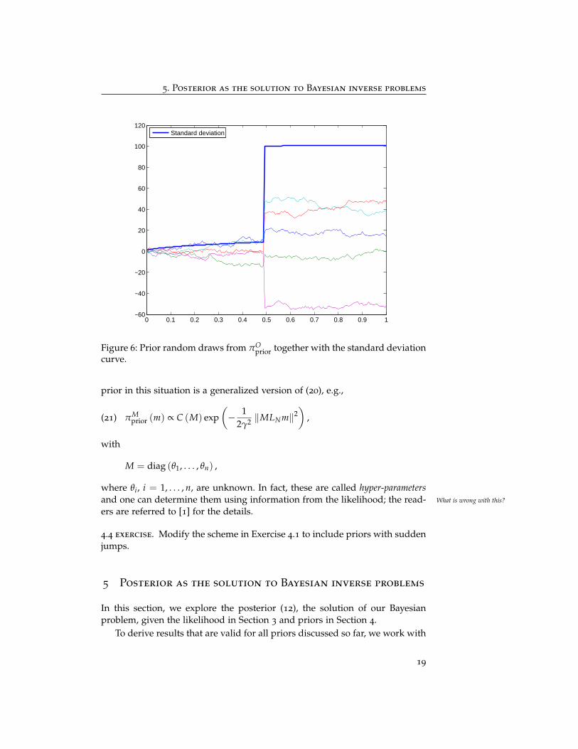
Let’s draw some random realizations from πOprior (m) in Figure 6 with n = 160,

j = 80, β = 1, and θ = 0.01. As desired, all realizations have a sudden jumpat j = 80, and the standard deviation of the jump is 1/θ = 100. In addition,compared to priors in Figure 4 and 5, the realizations from πO

prior (m) are lesssmooth, which confirms that our belief is indeed conveyed.

4.3 exercise. Use BayesianPriorElicitation.m to construct examples with2 or more sudden jumps and plot a few random realizations to see whetheryour belief is conveyed.

A more interesting and more practical situation is the one in which wedon’t know how many jump discontinuities and their locations. A natural

18

5. Posterior as the solution to Bayesian inverse problems

0 0.1 0.2 0.3 0.4 0.5 0.6 0.7 0.8 0.9 1−60

−40

−20

0

20

40

60

80

100

120

Standard deviation

Figure 6: Prior random draws from πOprior together with the standard deviation

curve.

prior in this situation is a generalized version of (20), e.g.,

(21) πMprior (m) ∝ C (M) exp

(− 1

2γ2 ‖MLNm‖2)

,

with

M = diag (θ1, . . . , θn) ,

where θi, i = 1, . . . , n, are unknown. In fact, these are called hyper-parametersand one can determine them using information from the likelihood; the read- What is wrong with this?

ers are referred to [1] for the details.

4.4 exercise. Modify the scheme in Exercise 4.1 to include priors with suddenjumps.

5 Posterior as the solution to Bayesian inverse problems

In this section, we explore the posterior (12), the solution of our Bayesianproblem, given the likelihood in Section 3 and priors in Section 4.

To derive results that are valid for all priors discussed so far, we work with

19


the following generic prior

πprior (m) ∝ exp(− 1

2γ2

∥∥∥Γ−12 m∥∥∥2)

,

where Γ−12 ∈ LD, LA, HLN, each of which again presents a different belief.

The Bayesian solution (12) can be now written as

πpost

(m|yobs

)∝ exp

−[

12σ2

∥∥∥yobs −Am∥∥∥2

+1

2γ2

∥∥∥Γ−12 m∥∥∥2]

︸︷︷︸T(m)

,

where T (m) is the familiar (to you I hope) Tikhonov functional; it is sometimescalled the potential. We re-emphasize here that the Bayesian solution is theposterior probability density, and if we draw samples from it, we want toknow what the most likely function m is going to be. In other words, weask for the most probable point m in the posterior distribution. This point isknown as the Maximum A Posteriori (MAP) estimator/point, namely, the pointat which the posterior density is maximized. Let us denote this point as mMAP,and we have

mMAPdef= arg max

mπpost

(m|yobs

)= arg min

mT (m) .

Hence, the MAP point is exactly the deterministic solution of the Tikhonovfunctional!

Since both likelihood and prior are Gaussian, the posterior is also a Gaus-sian. For our case, the resulting posterior Gaussian readsThis is fundamental. If you have not seen

this, prove it!

πpost

(m|yobs

)∝ exp

(−1

2

∥∥∥∥m− 1σ2 H−1ATyobs

∥∥∥∥2

H

)

= exp(−1

2

(m− 1

σ2 H−1ATyobs, H(

m− 1σ2 H−1ATyobs

)))def= exp

(−1

2

(m− 1

σ2 H−1ATyobs, Γ−1post

(m− 1

σ2 H−1ATyobs)))

where

H = 1σ2ATA+ 1

γ2 Γ−1 ,

is the Hessian of the Tikhonov functional (aka the regularized misfit), and we

have used the weighted norm ‖·‖2H =

∥∥∥H12 ·∥∥∥2

.

20


5.1 exercise. Show that the posterior is indeed a Gaussian, i.e.,

πpost

(m|yobs

)∝ exp

(−1

2

∥∥∥∥m− 1σ2 H−1ATyobs

∥∥∥∥2

H

).

The other important point is that the posterior covariance matrix is pre-cisely the inverse of the Hessian of the regularized misfit, i.e.,

Γpost = H−1 .

Last, but not least, we have showed that the MAP point is given by

mMAP =1σ2 H−1ATyobs =

1σ2

(1σ2A

TA+1

γ2 Γ−1)−1ATyobs,

which is, again, exactly the solution of the Tikhonov functional for linear in-verse problem.

5.2 exercise. Show that mMAP is also the least squares solution of the follow-ing over-determined system[

1σA

1γ Γ−

12

]m =

[ 1σ yobs

0

]5.3 exercise. Show that the posterior mean, which is in fact the conditionalmean, is precisely the MAP point.

Since the covariance matrix, generalization of the variance in multi-dimensionalspaces, represents the uncertainty, quantifying the uncertainty in the MAP es-timator is ready by simply computing the inverse the Hessian matrix. Let’s usnow numerically explore the Bayesian posterior solution.

We choose β = 0.05, n = 100, and γ = 1/n. The truth underlying functionthat we would like to invert for is given by

f (t) = 10(t− 0.5) exp(−50(t− 0.5)2

)− 0.8 + 1.6t.

The noise level is taken to be the 5% of the maximum value of f (s), i.e. σ =0.05 maxs∈[0,1] | f (s)|.

We first consider the belief described by πDprior in which we think that

f (s) is zero at the boundaries. Figures 7 plots the MAP estimator, the truthfunction f (s), and the predicted uncertainty. As can be observed, the MAP isin good agreement with the truth function inside the interval [0, 1], thoughit is far from recovering f (s) at the boundaries. This is the price we have topay for not admitting our ignorance about the boundary values of f (s). The

21


likelihood in fact sees this discrepancy in the prior knowledge and tries tomake correction by lifting the MAP away from 0, but not enough to be a goodreconstruction. The reason is that our incorrect prior is strong enough suchthat the information from the data yobs cannot help much.

0 0.1 0.2 0.3 0.4 0.5 0.6 0.7 0.8 0.9 1−1

−0.8

−0.6

−0.4

−0.2

0

0.2

0.4

0.6

0.8

1

MAP

truth

uncertainty

Figure 7: The MAP estimator, the truth function, and the predicted uncertainty(95% credibility region) using πD

prior.

5.4 exercise. Can you make the prior less strong? Change some parameter tomake prior contribution less! Use BayesianPosterior.m to test your answer. Isthe prediction better in terms of satisfying the boundary conditions? Is theuncertainty smaller? If not, why?

On the other hand, if we admit this ignorance and use the correspondingprior πD

prior, we see much better reconstruction in Figure 8. In this case, we in

fact let the information from the data yobs determine the appropriate valuesfor the Dirichlet boundary conditions rather than setting them to zero. Bydoing this, we allow the likelihood and the prior to be well-balanced leadingto good reconstruction and uncertainty quantification.

5.5 exercise. Play with BayesianPosterior.m by varying γ, the data misfit(or the likelihood) contribution, and σ, the regularization (or the prior) contri-bution.

22


0 0.1 0.2 0.3 0.4 0.5 0.6 0.7 0.8 0.9 1−1

−0.8

−0.6

−0.4

−0.2

0

0.2

0.4

0.6

0.8

1

MAP

truth

uncertainty

Figure 8: The MAP estimator, the truth function, and the predicted uncertainty(95% credibility region) using πA

prior.

5.6 exercise. Use your favorite deterministic inversion approach to solve theabove deconvolution problem and then compare it with the solution in Figure8.

Now consider the case in which the truth function has a jump discontinuityat j = 70. Assume we also know that the magnitude of the jump is 10. Inparticular, we take the truth function f (s) as the following step function

f (s) =

0 if s ≤ 0.710 otherwise

.

Since we otherwise have no further information about f (s), let us be moreconservative by choosing γ = 1 and θ = 0.1 at j = 70 in πO

prior as we discussedin (20). Figure 9 shows that we are doing pretty well in recovering the jumpand other parts of the truth function.

A question you may ask is whether we can do better? The answer is yes bytaking smaller γ if the truth function does not vary much everywhere except at Why?

the jump discontinuity. We take this prior information into account by takingγ = 1.e− 8, for example, then our reconstruction is almost perfect in Figure10.

23

6. Connection between Bayesian inverse problems and deterministic

inverse problems

0 0.1 0.2 0.3 0.4 0.5 0.6 0.7 0.8 0.9 1−4

−2

0

2

4

6

8

10

12

14

MAP

truth

uncertainty

Figure 9: The MAP estimator, the truth function, and the predicted uncertainty(95% credibility region) using πO

prior.

5.7 exercise. Try BayesianPosteriorJump.m with γ deceasing from 1 to 1.e−8 to see the improvement in quality of the reconstruction.

5.8 exercise. Use your favorite deterministic inversion approach to solve theabove deconvolution problem with discontinuity and then compare it withthe solution in Figure 10.

6 Connection between Bayesian inverse problems and

deterministic inverse problems

We have touched upon the relationship between Bayesian inverse problemand deterministic inverse problem in Section 5 by pointing out that the po-tential of the posterior density is precisely the Tikhonov functional up to aconstant. We also point out that the MAP estimator is exactly the solution ofthe deterministic inverse problem. Note that we derive this relation for a lin-ear likelihood model, but it is in fact true for nonlinear ones (e.g. nonlinearparameter-to-observable map Am).Can you confirm this?

Up to this point, you may realize that the Bayesian solution contains muchmore information than its deterministic counterpart. Instead of having a pointestimate, the MAP point, we have a complete posterior distribution to explore.In particular, we can talk about a simple uncertainty quantification by exam-

24


inverse problems

0 0.1 0.2 0.3 0.4 0.5 0.6 0.7 0.8 0.9 1−2

0

2

4

6

8

10

12

MAP

truth

uncertainty

Figure 10: The MAP estimator, the truth function, and the predicted uncer-tainty (95% credibility region) using πO

prior.

ining the diagonal of the posterior covariance matrix. We can even discussabout the posterior correlation structure by looking at the off diagonal ele-ments, though we are not going to do it here in this lecture note. Since, again,both likelihood and prior are Gaussian, the posterior is a Gaussian distribu-tion, and hence the MAP point (the first order moment) and the covariancematrix (the second order moment) are the complete description of the poste-rior. If, however, the likelihood is not Gaussian, say when the Am is nonlinear,then one can explore higher moments.

We hope the arguments above convince you that the Bayesian solution pro-vide information far beyond the deterministic counterpart. In the remainderof this section, let us dig into details the connection between the MAP pointand the deterministic solution, particularly in the context of the deconvolutionproblem. Recall the definition of the MAP point

mMAPdef= arg min

mT (m) = σ2

(12

∥∥∥yobs −Am∥∥∥2

+12

σ2

γ2

∥∥∥Γ−12 m∥∥∥2)

= arg minm

T (m) = σ2(

12

∥∥∥yobs − y∥∥∥2

+12

κ∥∥∥R

12 m∥∥∥2)

,

where we have defined κ = σ2/γ2, R12 = Γ−

12 , and y = Am.

We begin our discussion with zero Dirichlet boundary condition prior

25


inverse problems

πDprior (m) in (17). Recall in (14) and (16) that LD M is proportional to a dis-

cretization of the Laplacian operator with zero boundary conditions usingsecond order finite difference method. Therefore, our Tikhonov functional isin fact a discretization, up to a constant, of the following potential in the infi-nite dimensional setting

T∞ ( f ) =12

∥∥∥y− yobs∥∥∥2

+12

κ ‖∆ f ‖2L2(0,1) ,

where ‖·‖2L2(0,1)

def=∫ 1

0 (·)2 ds. Rewrite the preceding equation informally as

T∞ ( f ) =12

∥∥∥y− yobs∥∥∥2

+12

κ(

f , ∆2 f)

L2(0,1),

and we immediately realize that the potential in our prior description, namely‖LDm‖2, is in fact a discretization of Tikhonov regularization using the bihar-monic operator. This is another explanation for the smoothness of the priorrealizations and the name smooth prior, since biharmonic regularization isvery smooth. 13

The power of the statistical approach lies in the construction of priorπR

prior (m). Here, the interpretation of rows corresponding to interior nodessj is still the discretization of the biharmonic regularization, but the designof those corresponding to the boundary points is purely statistics, for whichwe have no corresponding deterministic counterpart (or at least it is not clearhow to construct it from a purely deterministic point of view). As the resultsin Section 5 showed, πR

prior (m) provided much more satisfactory results bothin the prediction and in uncertainty quantification.

As for the “non-smooth”priors in Section 4.2, a simple inspection showsthat LNm is, up to a constant, a discretization of ∇ f . Similar to the above dis-cussion, the potential in our prior description, namely ‖LDm‖2, is now in facta discretization of Tikhonov regularization using the Laplacian operator.14 Asa result, the current prior is less smooth than the previous one with harmonicoperator. Nevertheless, all the prior realizations corresponding to πpren (m)

13From a functional analysis point of view, ‖∆ f ‖2L2(0,1) is finite if f ∈ H2 (0, 1), and by Sobolev

imbedding theorem we know that in fact f ∈ C1,1/2−ε, the space of continuous differentialfunctions whose first derivative is in the Hölder space of continuous function C1/2−ε, for any0 < ε < 1

2 . So indeed f is more than continuously differentiable.14Again, Sobolev embedding theorem shows that f ∈ C1/2−ε for ‖∇ f ‖2

L2(0,1) to be finite. Hence,

all prior realizations corresponding to πpren (m) are at least continuous. The prior πOprior (m) is

different, due to the scaling matrix J. As long as θ stays away from zero, prior realizations arestill in H1 (0, 1), and hence continuous though having steep gradient at sj as shown in Figures 9

and 10. But as θ approaches zero, prior realizations are leaving H1 (0, 1), and therefore may be no

longer continuous. Note that in one dimension, H12 +ε is enough to be embedded in the space of

Cε-Hölder continuous functions. If you like to know a bit about the Sobolev embedding theorem,see [3].

26

7. Markov chain Monte Carlo

are at least continuous, though may have steep gradient at sj as shown in Fig-ures 9 and 10. The rigorous arguments for the prior smoothness require theSobolev embedding theorem, but we avoid the details.

For those who have not seen the Sobolev embedding theorem, you onlyloose the insight on why πO

prior (m) could give very steep gradient realizations(which is the prior belief we start with). Nevertheless, you still can see thatπO

prior (m) gives less smooth realizations than πDprior (m) does, since, at least,

the MAP point corresponding to πOprior (m) only requires finite first deriva-

tive of f while second derivative of f needs to be finite at the MAP point ifπD

prior (m) is used.

7 Markov chain Monte Carlo

In the last section, we have shown that if the paramter-to-observable map islinear, i.e. h (m) = Am, and both the noise and the prior models are Gaus-sian, then the MAP point and the posterior covariance matrix are exactly thesolution and the inverse of the Hessian of the Tikhonov functional, respec-tively. Moreover, since the posterior is Gaussian, the MAP point is identicallythe mean, and hence the posterior distribution is completely characterized. Inpractice, h (m) is typically nonlinear. Consequently, the posterior distributionis no longer Gaussian. Nevertheless, the MAP point is still the solution of theTikhonov functional, though the mean and the convariance matrix are to bedetermined. The question is how to estimate the mean and the covariancematrix of a non-Gaussian density.

We begin by recalling the definition the mean

m = E [M] ,

and a natural idea is to approximate the integral by some numerical inte-gration. For example, suppose S = [0, 1] and then we can divide S into Nintervals, each of which has length of 1/N. Using a rectangle rule gives

(22) m ≈ (M1 + . . . + MN)

N.

But this kind of method cannot be extended to S = Rn. This is where thecentral limit theorem and law of large numbers come to rescue. They say thatthe simple formula (22) is still valid with a simple error estimation expression.

7.1 Some classical limit theorems

7.1 theorem (central limit theorem (CLT)). Assume that real valued random vari-ables M1, . . . are independent and identically distributed (iid), each with expectation

27


m and variance σ2. Then

ZN =1

σ√

N(M1 + M2 + · · ·+ MN)−

mσ

√N

converges, in distribution15, to a standard normal random variable. In particular,

(23) limN→∞

P [ZN ≤ m] =1

2π

m∫−∞

exp(− t2

2

)dt

Proof. The proof is elementary, though technical, using the concept of charac-teristic function (Fourier transform of a random variable). You can consult [4]for the complete proof.

7.2 theorem (Strong law of large numbers (LLN)). Assume random variablesM1, . . . are independent and identically distributed (iid), each with finite expectationm and finite variance σ2. Then

(24) limN→∞

SN =1N

(M1 + M2 + · · ·+ MN) = m

almost surely16.

Proof. A beautiful, though not classical, proof of this theorem is based onbackward martingale, tail σ-algebra, and uniform integrability. Let’s accept itin this note and see [4] for the complete proof.

7.3 remark. The central limit theorem says that no matter what the underly-ing common distribution looks like, the sum of iid random variables, whenproperly scaled and centralized, converges in distribution to a standard nor-mal distribution. The strong law of large numbers, on the other hand, statesthat the average of the sum is, as expected in the limit, precisely the mean ofthe common distribution with probability one.

Both the central limit theorem (CLT) and the strong law of large numbers(LLN) are useful, particularly LLN, and we use them routinely. For example,if you are given an iid sample M1, M2, · · · , MN from a common distribu-tion π (m), the first thing you should do is to compute the the sample meanSN to estimate the actual mean m. From LLN we know that the sample meancan be as close as desired if N is sufficiently large. A question immediatelyarises is whether we can estimate the error between the sample mean and the

15Convergence in distribution is also known as weak convergence and it is beyond the scope ofthis introductory note. You can think of the distribution of Zn is more and more like the standardnormal distribution as n→ ∞, and it is precisely (23).

16Almost sure convergence is the same as convergence with probability one, that is, the eventon which the convergence (24) does not happen has zero probability.

28


truth mean, given a finite N. Let us first give an answer based on a simpleapplication of the CLT. Since the sample M1, M2, · · · , MN satisfies the con-dition of the CLT, we know that ZN converges to N (0, 1). It follows that, atleast for sufficiently large N, the mean squared error between zN and 0 can beestimated as

‖zN − 0‖2L2(S,P)

def= E

[(zN − 0)2

]def= Var [ZN − 0] ≈ 1,

which, after some simple algebra manipulations, can be rewritten as

(25) ‖SN −m‖2L2(S,P)

def= Var [SN −m] ≈ σ2

N

7.4 exercise. Show that (25) holds.

7.5 remark. The result (25) shows that the error of the sample mean SN in theL2 (S, P)-norm goes to zero like 1/

√N. One should be aware of the popular

statement that the error goes to zero like 1/√

N independent of dimension isnot entirely correct because the variance σ2, and hence the standard deviationσ, of the underlying distribution π (m) may depend on the dimension n.

If you are a little bit delicate, you may not feel completely comfortable withthe error estimate (25) since you can rewrite it as

‖SN −m‖L2(S,P) = Cσ√N

,

and you are not sure how big C is and the dependence of C on N. Let us tryto make you happy. We have

‖SN −m‖2L2(S,P) =

1N2 E

[(N

∑i=1

(Mi −m)

)(N

∑j=1

(Mj −m

))]

=1

N2 E

[(N

∑i=1

(Mi −m)2

)]=

1N2

N

∑i=1

σ2 =σ2

N,

where we have used m = 1N ∑N

i=1 m in the first equality, E[(Mi −m)

(Mj −m

)]=

0 if i 6= j in the second equality since Mi, i = 1, . . . , N are iid random variables,and the definition of variance in the third equality. So in fact C = 1, and wehope that you feel pleased by now.

In practice, we rarely work with M directly but indirectly via some map-ping g : S → T. We have that g (Mi), i = 1, . . . , N are iid17 if Mi, i = 1, . . . , Nare iid.

17We avoid technicalities here, but g needs to be a Borel function for the statement to be true.

29


7.6 exercise. Suppose the density of M is π (m) and z = g (m) is differentiallyinvertible, i.e. m = g−1 (z) exists and differentiable, what is the density ofg (M)?

Perhaps, one of the most popular and practical problems is to evaluate themean of g, i.e.,

(26) I def= E [G (M)] =

∫S

g (m)π (m) dm,

which is an integral in Rn.

7.7 exercise. Define z = g (m) ∈ T, the definition of the mean in (7) gives

E [G (M)] ≡ E [Z] def=∫T

zπZ (z) dz.

Derive formula (26).

Again, we emphasize that using any numerical integration methods thatyou know of for integral (26) is either infeasible or prohibitedly expensivewhen the dimension n is large, and hence not scalable. The LLN provides areasonable answer if we can draw iid samples g (M1) , . . . , g (MN) since weknow that

limN→∞

1N

(g (M1) + . . . + g (MN))︸︷︷︸IN

= I

with probability 1. Moreover, as showed above, the mean squared error isgiven byDo you trivially see this?

‖IN − I‖2L2(T,P) = E

[(IN − I)2

]=

Var [G (M)]

N.

Again, the error decreases to zero like 1/√

N “independent” of the dimensionof T, but we need to be careful with such a statement unless Var [G (M)]DOES NOT depend on the dimension.

A particular function g of interest is the following

g (m) = (m−m) (m−m)T ,

whose expectation is precisely the covariance matrix

Γ = cov (M) = E[(M−m) (M−m)T

]= E [G] .

30


The average IN in this case is known as the sample (aka empirical) covariancematrix. Denote

Γ =1N

N

∑i=1

(mi −m) (mi −m)T

as the sample covariance matrix. Note that m is typically not available in prac-tice, and we have to resort to a computable approximation

Γ =1N

N

∑i=1

(mi − m) (mi − m)T ,

with m denoting the sample mean.

7.2 Independent and identically distributed random draws

Sampling methods discussed in this note are based on two fundamental iidrandom generators that are available as built-in functions in Matlab. The firstone is rand.m function which can draw iid random numbers (vectors) fromthe uniform distribution in [0, 1], denoted as U [0, 1], and the second one israndn.m function that generates iid numbers (vectors) from standard normaldistribution N (0, I), where I is the identity matrix of appropriate size.

The most trivial task is how to draw iid samples M1, M2, . . . , MN from amultivariate Gaussian N (m, Γ). This can be done through a so-called whiten-ing process. The first step is to carry out the following decomposition

Γ = RRT ,

which can be done, for example, using Cholesky factorization. The secondstep is to define a new random variable as

Z = R−1 (M−m) ,

then Z is a standard multivariate Gaussian, i.e. its density isN (0, I), for which Show that Z is a standard multivariateGaussian.randn.m can be used to generate iid samples

Z1, Z2, . . . , ZN = randn(n,N).

We now generate iid samples Mi by solving

Mi = m + RZi.

7.8 exercise. Look at BayesianPriorElicitation.m to see how we apply theabove whitening process to generate multivariate Gaussian prior random re-alizations.

31


You may ask what if the distribution under consideration is not Gaussian,which is true for most practical applications. Well, if the target density π (m)is one dimensional or multivariate with independent components (in this case,we can draw samples from individual components separately), then we stillcan draw iid samples from π (m), but this time via the standard uniformdistribution U [0, 1]. If you have not seen it before, here is the definition: U [0, 1]has 1 as its density function, i.e.,

(27) µU (A) =∫A

ds, ∀A ⊂ [0, 1] .

Now suppose that we would like to draw iid samples from a one dimensional(S = R) distribution with density π (m) > 0. We still allow π (m) to be zero,but only at isolated points on R, and you will see the reason in a moment.Define the cumulative distribution function (CDF) as

(28) Φ (w) =

w∫−∞

π (m) dm,

then it is clearly that Φ(w) is non-decreasing and 0 ≤ Φ(w) ≤ 1. Let us defineWhy?

a new random variable Z as

(29) Z = Φ (M) .

Our next step is to prove that Z is actually a standard uniform random vari-able, i.e. Z ∼ U [0, 1], and then show how to draw M via Z. We begin by thefollowing observation

(30) P [Z < a] = P [Φ (M) < a] = P[

M < Φ−1 (a)]=

Φ−1(a)∫−∞

π (m) dm,

where we have used (29) in the first equality, the monotonicity of Φ (M) in thesecond equality, and the definition of CDF (28) in the last equality. Now, wecan view (29) as the change of variable formula z = Φ (m), then combiningthis fact with (28) to have

dz = dΦ (m) = π (m) dm, and z = a when x = Φ−1 (a) .

Consequently, (30) becomesDo you see the second equality?

P [Z < a] =a∫

−∞

dz = µZ (Z < a) ,

32


which says that the density of Z is 1, and hence Z must be a standard uniformrandom variable. In terms of our language at the end of Section 7.1, we candefine M = g (Z) = Φ−1 (Z), then drawing iid samples for M is simple by firstdrawing iid samples from Z, then mapping them through g. Let us summarizethe idea in Algorithm 1.

Algorithm 1 CDF-based sampling algorithm

1. Draw z ∼ U [0, 1],

2. Compute the inverse of the CDF to draw m, i.e. m = Φ−1 (z). Go backto Step 1.

The above method works perfectly if one can compute the analytical in-verse of the CDF easily and efficiently; it is particularly efficient for discreterandom variables, as we shall show. You may say that you can always computethe inverse CDF numerically. Yes, you are right, but you need to be carefulabout this. Note that the CDF is an integral operation, and hence its inverseis some kind of differentiation. The fact is that numerical differentiation is anill-posed problem! You don’t want to add extra ill-posedness on top of theoriginal ill-posed inverse problem that you started with, do you? If not, let usintroduce to you a simpler but more robust algorithm that works for multi-variate distribution without requiring the independence of individual compo-nents. We shall first introduce the algorithm and then analyze it to show youwhy it works.

Suppose that you want to draw iid samples from a target density π (m),but you only know it up to a constant C > 0, that is, you only know Cπ (m).(This is perfect for our Bayesian inversion framework since we typically knowthe posterior up to a constant as in (12).) Assume that we have a proposal distri-bution q (m) at hand, for which we know how to sample easily and efficiently.This is not a limitation since we can always take either the standard normaldistribution or uniform distribution as the proposal distribution. We furtherassume that there exists D > 0 such that

(31) Cπ (m) ≤ Dq (m) ,

then we can draw a sample from π (m) by the rejection-acceptance samplingAlgorithm 2.

In practice, we carry out Step 3 of Algorithm 2 by flipping an “α-coin”. Inparticular, we draw u from U [0, 1], then accept m if α > u. It may seem to bemagic to you why Algorithm 2 provides random samples from π (m). Let usconfirm this with you using the Bayes formula (9).

7.9 proposition. Accepted m is distributed by the target density π.

33


Algorithm 2 Rejection-Acceptance sampling algorithm

1. Draw m from the proposal q (m),

2. Compute the acceptance probability

α =Cπ (m)

Dq (m),

3. Accept m with probability α or reject it with probability 1− α. Go backto Step 1.

Make sure you understand this proof sincewe will reuse most of it for the Metropolis-Hastings algorithm!

Proof. Denote B as the event of accepting a draw q (or the acceptance event).Algorithm 2 tells us that the probability of B given m, which is precisely theacceptance probability, is

(32) P [B|m] = α =Cπ (m)

Dq (m).

On the other hand, the prior probability of m in the incremental event dA =[m′, m′ + dm] in Step 1 is q (m) dm. Applying the Bayes formula for conditionalprobability (4) yields the distribution of a draw m provided that it has beenalready accepted

P [m ∈ dA|B] = P [B|m] q (m) dmP [B]

= π (m) dm,

where we have used (32) and P [B], the probability of accepting a draw fromq, is the following marginal probability

P [B] =∫S

P [B|m] q (m) dm =CD

∫S

π (m) dm =CD

.

Note that

P [B, m ∈ dm] = π (B, m) dm = P [B|m]πprior (m) = P [B|m] q (m) dm,

an application of (3), is the probability of the joint event of drawing an m fromq (m) and accept it. The probability of B, the acceptance event, is the total ofaccepting probability, which is exactly the marginal probability. As a result,we have

P [m ∈ A|B] =∫A

π (m) dm,

34


which, by definition (6), says that the accepted m in Step 3 of Algorithm 2 isdistributed by π (m), and this is the desired result.

Algorithm 2 is typically slow in practice in the sense that a large portionof samples is rejected, particularly for high dimensional problem, though itprovides iid samples from the true underlying density. Another problem withthis algorithm is the computation of D. Clearly, we can take very large D andthe condition (31) would be satisfied. However, the larger D is the smaller theacceptance probability α, making Algorithm 2 inefficient since most of drawsfrom q (m) will be rejected. As a result, we need to minimize D and this couldbe nontrivial depending the complexity of the target density.

7.10 exercise. You are given the following target density

π (m) =g (m)

Cexp

(−m2

2

),

where C is some constant independent of m, and

g (m) =

1 if x > a0 otherwise

, a ∈ R.

Take the proposal density as q (m) = N (0, 1).

1. Find the smallest D that satisfies condition (31).

2. Implement the rejection-acceptance sampling Algorithm 2 in Matlab anddraw 10000 samples, by taking a = 1. Use Matlab hist.m to plot thehistogram. Does its shape resemble the exact density shape?

3. Increase a as much as you can, is there any problem with Algorithm 2?Can you explain why?

7.11 exercise. You are given the following target density

π (m) ∝ exp

(− 1

2σ2

(√m2

1 + m22 − 1

)2− 1

2δ2 (m2 − 1)2

),

where σ = 0.1 and δ = 1. Take the proposal density as q (m) = N (0, I2),where I2 is the 2× 2 identity matrix.

1. Find a reasonable D, using any means you like, that satisfies condition(31).

2. Implement the rejection-acceptance sampling Algorithm 2 in Matlab anddraw 10000 samples. Plot a contour plot for the target density, and youshould see the horse-shoe shape, then plot all the samples as dots on topof the contour. Do most of the samples sit on the horse-shoe?

35


7.3 Markov chain Monte Carlo

We have presented a few methods to draw iid samples from a target distri-bution q (m). The most robust method that works in any dimension is therejection-acceptance sampling algorithm though it may be slow in practice.In this section, we introduce the Markov chain Monte Carlo scheme whichis the most popular sampling approach. It is in general more effective thanany methods discussed so far, particularly for complex target density in highdimensions, though it has its own problems. One of them is that we no longerhave iid samples but correlated ones. Let us start the motivation by consider-ing the following web-page ranking problem.

Assume that we have a set of Internet websites that may be linked to theothers. We represent these sites as nodes and mutual linkings by directed ar-rows connecting nodes such as in Figure 11. Now you are seeking sites that

1

2

3

5

4

Figure 11: Five internet websites and their connections.

contains a keyword of interest for which all the nodes, and hence websites,contain. A good search engine will show you all these websites. The questionis now which website should be ranked first, second, and so on? You mayguess that node 4 should be the first one in the list. Let us present a proba-bilistic method to see whether your guess is correct or not. We first assign the

36


network of nodes a transition matrix P as

(33) P =

0 1 0 1/3 0

1/2 0 0 1/3 00 0 0 0 1/2

1/2 0 1/2 0 1/20 0 1/2 1/3 0

.

The jth column of P is contains the probability of moving from the jth nodeto the rest. For example, the first column says that if we start from node 1, wecan move to either node 2 or node 4, each with probability 1

2 . Note that wehave treated all the nodes equally, that is, the transition probability from onenode to other linked nodes is the same (a node is not linked to itself in thismodel). Note that the sum of each column is 1, meaning that a website musthave a link to a website in the network.

Assume we are initially at node 4, and we represent the initial probabilitydensity as

π0 =

00010

,

that is, we are initially at node 4 with certainty. In order to know the next nodeto visit, we first compute the probability density of the next state by

π1 = Pπ0,

then randomly move to a node by drawing a sample from the (discrete) prob-ability density πj (see Exercise 7.12). In general, the probability density afterk steps is given by

(34) πk = Pπk−1 = . . . = Pkπ0,

where the jth component of πk is the probability of moving to the jth node.

Observing (34) you may wonder what happens if k approaches infinity.Assume, on credit, the limit probability density π∞ exists, then it ought tosatisfy

(35) π∞ = Pπ∞.

It follows that π∞ is the “normalized” eigenvector of P corresponding to unityeigenvalue. Here, normalization means taking that eigenvector and then di-viding by the sum of its components so that the result is a probability density.

37


Figure 12 shows the visiting frequency (blue) for each node after N = 1500moves. Here, visiting frequency of a node is the number of visits to that nodedivided by N. We expect that numerical visiting frequencies approximate thevisiting probabilities in the limit. We confirm this expectation by also plottingthe components of π∞ (red) in Figure 12. By the way, π1500 is equal to π∞ upto machine zero, meaning that a draw from πN , N ≥ 1500, is distributed bythe limit distribution π∞. We are now in the position to answer our rankingquestion. Figure 12 shows that node 1 is the most visited one, and henceshould appear at the top of the website list coming from the search engine.

1 2 3 4 50

0.05

0.1

0.15

0.2

0.25

0.3

0.35

visiting frequencyfirst eigenvector

Figure 12: Visiting frequency after N = 1500 moves and the first eigenvector.

7.12 exercise. Use the CDF-based sampling algorithm, namely Algorithm 1,to reproduce Figure 12. Compare the probability density π1500 with the limitdensity, are they the same? Generate 5 figures corresponding to starting nodes1, . . . , 5, what do you observe?

7.13 exercise. Using the above probabilistic method to determine the proba-bility that the economy, as shown in Figure 13, is in recession.

The limit probability density π∞ is known as the invariant density. Invari-ance here means that the action of P on π∞ returns exactly π∞. In summary,we start with the transition matrix P and then find the invariant probabilitydensity by taking the limit. Drawings from πk are eventually distributed as theinvariant density (see Exercise 7.12). A Markov chain Monte Carlo (MCMC)

38


Figure 13: Economy states extracted fromhttp://en.wikipedia.org/wiki/Markov_chain

method reverses the process. In particular, we start with a target densityand look for the transition matrix such that MCMC samples are eventuallydistributed as the target density. Before presenting the popular Metropolis-Hastings MCMC method, we need to explain what “Markov” means.

Let us denote m0 = 4 the initial starting node, then the next move m1 iseither 1 or 2 or 5 since the probability density is

(36) π1(m1|m0) = [1/3, 1/3, 0, 0, 1/3]T ,

where we have explicitly pointed out that π1 is a conditional probability den-sity given known initial state m0. Similarly, (34) should have been written as

πk (mk|m0) = Pπk−1 (mk−1|m0) = . . . = Pkπ0.

Now assume that we know all states up to mk−1, say mk−1 = 1. It follows that

πk−1 (mk−1|mk−2, . . . , m0) = [1, 0, 0, 0, 0]T ,

since we know mk−1 for certain. Consequently,

πk (mk|mk−1, . . . , m0) = Pπk−1 (mk−1|mk−2, . . . , m0) = P [1, 0, 0, 0, 0]T

39


regardless of the values of the states mk−2, . . . , m0. More generally,

πk (mk|mk−1, . . . , m0) = πk (mk|mk−1) ,

which is known as Markov property, namely, “tomorrow depends on the pastonly through today”.

7.14 definition. A collection m0, m1, . . . , mN , . . . is called Markov chain if thedistribution of mk depends only on the immediate previous state mk−1.

Next, let us introduce some notations to study MCMC methods.

7.15 definition. We call the probability of mk in A starting from mk−1 as thetransition probability and denote it as P (mk−1, A). With an abuse of notation,we introduce the transition kernel P (mk−1, m) such thatWhat does P (mk−1, dm) mean?

P (mk−1, A)def=∫A

P (mk−1, m) dm =∫A

P (mk−1, dm) .

Clearly P (m, S) =∫

S P (m, p) dp = 1.

7.16 example. Let mk−1 = 4 in our website ranking problem, then the proba-bility kernel P (mk−1 = 4, m) is exactly the probability density in (36).What is the transition probability

P (mk−1 = 4, mk = 1)?

7.17 definition. We call µ (dm) = π (m) dm the invariant distribution andπ (m) invariant density of the transition probability P (mk−1, dm) if

(37) µ (dm) = π (m) dm =∫S

P (p, dm)π (p) dp.

7.18 example. The discrete version of (37), applying to our website rankingproblem, reads

π∞ (j) =5

∑k=1

P (j, k)π∞ (k) = P(j, :)π∞, ∀j = 1, . . . , 5,

which is exactly (35).

7.19 definition. A Markov chain m0, m1, . . . , mN , . . . is reversible if

(38) π (m) P (m, p) = π (p) P (p, m) .

The reversibility relation (38) is also known as detailed balanced equation.You can think of the reversibility saying that the probability of moving fromm to p is equal to the probability of moving from p to m.

40


7.20 exercise. What is the discrete version of (38)? Does the transition matrixin the website ranking problem satisfy the reversibility? If not, why? Howabout the transition matrix in Exercise 7.13.

The reversibility of a Markov chain is useful since we can immediatelyconclude that π (m) is its invariant density.

7.21 proposition. If the Markov chain m0, m1, . . . , mN , . . . is reversible with re-spect to π (m), then π (m) is the invariant density.

Proof. We need to prove (37), but it is straightforward since∫S

π (p) P (p, dm) dpreversibility

= π (m) dm∫S

P (m, p) dp = π (m) dm.

The above discussion shows that if a Markov chain is reversible then even-tually the states in the chain are distributed by the underlying invariant dis-tribution. A question you may ask is how to construct a transition kernel suchthat reversibility holds. This is exactly the question Markov chain Monte Carlomethods are designed to answer. Let us now present the Metropolis-HastingsMCMC method in Algorithm 3.

Algorithm 3 Metropolis-Hastings MCMC AlgorithmChoose initial m0for k = 0, . . . , N do

1. Draw a sample p from the proposal density q(mk, p )

2. Compute π(p), q(mk, p), and q(p, mk)

3. Compute the acceptance probability

α(mk, p) = min

1,π(p)q(p, mk)

π(mk)q(mk, p)

4. Accept and set mk+1 = p with probability α(mk, p). Otherwise,

reject and set mk+1 = mk

end for

The idea behind the Metropolis-Hastings Algorithm 3 is very similar tothat of rejection-acceptance sampling algorithm. That is, we first draw a sam-ple from an “easy” distribution q (mk, p), then make correction so that it isdistributed more like the target density π(p). However, there are two main

41


differences. First, the proposal distribution q (mk, p) is a function of the laststate mk. Second, the acceptance probability involves both the last state mkand the proposal move p. As a result, a chain generated from Algorithm 3 isin fact a Markov chain.

What remains to be done is to show that the transition kernel of Algorithm3 indeed satisfies the reversibility condition (38). This is the focus of the nextproposition.

7.22 proposition. Markov chains generated by Algorithm 3 are reversible.

Proof. We proceed in two steps. In the first step, we consider the case in whichthe proposal p is accepted. Denote B as the event of accepting a draw q (or theacceptance event). Following the same proof of Proposition 7.9, we have

P [B|p] = α(mk, p),

leading toMake sure you see this!

π (B, p) = P [B|p]πprior (p) = α(mk, p)q (mk, p) ,

which is exactly P (mk, p), the probability density of the joint event of drawingp from q (mk, p) and accept it, starting from mk. It follows that the reversibilityholds since

π (mk) P (mk, p) = π (mk) q (mk, p)min

1,π(p)q(p, mk)

π(mk)q(mk, p)

= min π(mk)q(mk, p), π(p)q(p, mk)

= min

π(mk)q(mk, p)π(p)q(p, mk)

, 1

π(p)q(p, mk)

= π (p) P (p, mk) .

In the second step, we remain at mk, i.e., mk+1 = mk, then the reversibilityis trivially satisfied no matter what the transition kernel P (mk, p) is. This isExplain why

the end of the proof.

7.23 exercise. What is the probability of staying put at mk?

As you can see the Metropolis-Hastings algorithm is simple and elegant,but provides us a reversible transition kernel, which is exactly what we arelooking for. The keys behind this are Steps 3 and 4 in Algorithm 3, knownas Metropolized steps. At this point, we should be able to implement thealgorithm except for one small detail: what should we choose for the proposal

42


density? Let us choose the following Gaussian kernel

q (m, p) =1√

2πγ2exp

(− 1

2γ2 ‖m− p‖2)

,

which is the most popular choice. Metropolis-Hastings algorithm with aboveisotropic Gaussian proposal is known as Random Walk Metropolis-Hastings (RWMH)algorithm. For this particular method, the acceptance probability is very sim-ple, i.e.,

α = min

1,π (p)π (m)

.

We are now in the position to implement the method. For concreteness, weapply the RWMH algorithm on the horse-shoe shape in Exercise 7.11. We takethe origin as the starting point m0. Let us first be conservative by choosing asmall proposal variance γ2 = 0.022 so that the proposal p is very close to thecurrent state mk. In order to see how the MCMC chain evolves, we plot eachstate mk as a circle (red) centered at mk with radius proportional to the numberof staying-puts. Figure 14(a) shows the results for N = 1000. We observe thatthe chain takes about 200 MCMC simulations to enter the high probabilitydensity region. This is known as burn-in time in MCMC literature, which tellsus how long a MCMC chain takes to start exploring the density. In otherwords, after the burn-in time, a MCMC begins to distribute like the targetdensity. As can be seen, the chain corresponding to small proposal varianceγ2 explores the target density very slowly. If we approximate the averageacceptance rate by taking the ratio of the number of accepted proposal overN, it is 0.905 for this case. That is, almost all the proposals p are accepted, butexploring a very small region of high probability density.

−1.5 −1 −0.5 0 0.5 1 1.5−1.5

−1

−0.5

0

0.5

1

1.5

(a) γ = 0.02

−1.5 −1 −0.5 0 0.5 1 1.5−1.5

−1

−0.5

0

0.5

1

1.5

(b) γ = 5

−1.5 −1 −0.5 0 0.5 1 1.5−1.5

−1

−0.5

0

0.5

1

1.5

(c) γ = 0.5

Figure 14: RWMH with different proposal variance γ2.

Let us now increase the proposal stepsize γ to 5, and we show the corre-sponding chain in Figure 14(b). This time, the chain immediately explores the

43


target density without any burn-in time. However, it does so in an extremelyslow manner. Most of the time the proposal p is rejected, resulting in a fewbig circles in Figure 14(b). The average acceptance rate in this case is 0.014,which shows that most of the time we reject proposals p.

The results in Figures 14(a) and 14(b) are two extreme cases, both of whichexplore the target density in a very lazy manner since the chain either acceptsall the small moves with very high acceptance rate or rejects big moves withvery low acceptance rate. This suggests that there must be an optimal accep-tance rate for the RWMH algorithm. Indeed, one can show that the optimalacceptance rate is 0.234 [5]. For our horse-shoe target, it turns out that thecorresponding optimal stepsize is approximately γ = 0.5. To confirm this, wegenerate a new chain with this stepsize, again with N = 1000, and show theresult in Figure 14(c). As can be seen, the samples spread out nicely over thehorse-shoe.

We have judged the quality and convergence of a MCMC chain by lookingat the scatter plot of the samples. Another simple approach is to look at thetrace plot of components of m. For example, we show the trace plot of thefirst component in Figure 15 for the above three stepsizes. The rule of thumbis that a Markov chain is considered to be good if its trace plot is close toa white noise one, a “fuzzy worm”, in which all the samples are completelyPlot a trace plot for a one dimensional

Gaussian white noise to see how it lookslike! uncorrelated. Based on this criteria, we again conclude that γ = 0.5 is the best

compared to the other two extreme cases.Nevertheless, the above two simple criteria are neither rigorous nor possi-

ble in high dimensions. This observation immediately reminds us the stronglaw of large number in computing the mean and its dimension-independenterror analysis using the central limit theorem. Since the target is symmetricabout the vertical axis, the first component of the mean must be zero. Let ususe the strong law of large number to estimate the means for the above threestepsizes and show them as cross signs in Figures 14(a), 14(b), and 14(c). Ascan be seen and expected, the sample mean for the optimal stepsize is the mostaccurate, though it is not exactly on the vertical axis since m1 = −0.038. Thisimplies that the sample size of N = 1000 is small. If we take N = 10000, thesample mean gives m1 = 0.003, signifying the convergence when N increases.Take N = 100000 for the optimal step-

size case, and again compute the samplemean using BayesianMCMC.m. Is the sam-ple mean better? If not, why?

However, the application of LLN and CLT is very limited for Markovchains since they don’t provide iid samples. Indeed, as in the above Markovchain theory, the states of the chain eventually identically distributed by π (m),but they are always correlated instead of independent since any state in thechain depends on the previous one. What we could hope for is that the cur-rent state is effectively independent from its kth previous state. In that case,the effective number of iid samples is N/k, and the mean square error, by thecentral limit theorem, decays as

√k/N. As the result, if k is large, the decay

rate is very slow. How to estimate k is the goal of the autocorrelation study, aswe now discuss.

44


0 1 2 3 4 5 6 7 8 9 10

x 104

−1.5

−1

−0.5

0

0.5

1

1.5

(a) γ = 0.02

0 1 2 3 4 5 6 7 8 9 10

x 104

−1.5

−1

−0.5

0

0.5

1

1.5

2

(b) γ = 5

0 1 2 3 4 5 6 7 8 9 10

x 104

−1.5

−1

−0.5

0

0.5

1

1.5

(c) γ = 0.5

Figure 15: Trace plots of the first component of m with different γ2.

45


We shall compute the autocorrelation for each component of m separately,therefore, without loss of generality, assume that m ∈ R1 and that the Markovchain

mjN

j=0 has zero mean. Consider the following discrete convolutionquantities

ck =N−k

∑j=0

mj+kmj, , k = 0, . . . , N − 1,

and define the autocorrelation of m with lag k as

ck =ckc0

, k = 0, . . . , N − 1.

If ck is zero, then we say that the correlation length of the Markov chain isapproximately k, that is, any state mj is considered to be insignificantly corre-lated to mj−k (and hence any state before mj−k), and to mj+k (and hence anystate after mj+k). In other words, every kth sample point can be considered tobe approximately independent. Note that this is simply a heuristic and oneshould be aware that independece implies un-correlation but not vice versa.

Let us now approximately compute the correlation length for three Markovchains corresponding to γ = 0.02, γ = 0.5, and γ = 5, respectively, withN = 100000. We first subtract away the sample mean as

zj = mj −1

N + 1

N

∑i=0

mi.

Then, we plot the autocorrelation functions ck for each component of the zeromean sample

zjN

j=0 in Figure 16. As can be observed, the autocorrelationlength for the chain with optimal stepsize γ = 0.5 is about k = 100, while theothers are much larger (not shown here). That is, every 100th sample point canbe considered to be independent for γ = 0.5. The case with γ = 0.02 is theworst, indicating slow move around the target density. The stepsize of γ = 5is better, but so big that the chain remains at each state for a long period oftime, and hence autocorrelation length is still significant relatively to that ofγ = 0.5.

Extensive MCMC methods including improvements on the standard RWMHalgorithm can be found in [6]. Let us introduce two simple modificationsthrough the following two exercises.

7.24 exercise. Consider the following target density

(39) π (m) ∝ exp(− 1

2δ2 ‖m‖2 − 1

2σ2 ‖y− h (m)‖2)

,

46

8. Matlab codes

where

h (m) =

[m2

1 −m2m2/5

], y =

[−0.20.1

].

Take δ = 1 and σ = 0.1.

1. Modify BayesianMCMC.m to simulate the target density in (39) with N =5000.

2. Tune the proposal stepsize γ so that the average acceptance probabilityis about 0.234. Show the scatter, trace, and autocorrelation plots for theoptimal stepsize.

7.25 exercise. So far the proposal density q (m, p) is isotropic and indepen-dent of the target density π (m). For anisotropic target density, isotropic pro-posal is not a good idea, intuitively. The reason is that the proposal is dis-tributed equally in all directions, whereas it is not in the target density. Anatural idea is to shape the proposal density to make it locally resemble thetarget density. A simple idea in this direction is to linearize h (m), and thendefine the proposal density as

q (mk, p) ∝ exp(− 1

2δ2 ‖p‖2 − 12σ2 ‖y− h (mk)−∇h (mk) (p−mk)‖2

),

1. Determine H (mk) such that q (mk, p) = N(

mk, H (mk)−1)

, by keepingonly the quadratic term in p−mk.

2. Modify BayesianMCMC.m to simulate the target density in (39) using the

proposal density q (mk, p) = N(

mk, H (mk)−1)

. Show the scatter, trace,and autocorrelation plots. Is it better than the isotropic proposal density?

7.26 exercise. Another idea to improve the standard RWMH algorithm is byadaptation. Let’s investigate a simple adaptation strategy. Use the resultingsample in Exercise 7.24 to compute the empirical covariance Γ, then use it toconstruct the proposal density q (m, p) = N

(m, Γ

). Show the scatter, trace,

and autocorrelation plots. Is it better than the isotropic proposal density?

8 Matlab codes

A set of Matlab codes that can be used to reproduce most of the figures in thenote can be downloaded from

http://users.ices.utexas.edu/~tanbui/teaching/Bayesian

47

References

References

[1] D. Calvetti and E. Somersalo. Introduction to Bayesian Scientific Computing:Ten Lectures on Subjective Computing. Springer, New York, 2007.

[2] Jari Kaipio and Erkki Somersalo. Statistical and Computational Inverse Prob-lems, volume 160 of Applied Mathematical Sciences. Springer-Verlag, NewYork, 2005.

[3] Todd Arbogast and Jerry L. Bona. Methods of Applied Mathematics. Univer-sity of Texas at Austin, 2008. Lecture notes in applied mathematics.

[4] Rick Durret. Probability: theory and examples. Cambidge University Press,2010.

[5] Gareth O. Roberts and Jeffrey S. Rosenthal. Optimal scaling for variousmetropolis-hastings algorithms. Statistical Science, 16(4):pp. 351–367, 2001.

[6] Christian P. Robert and George Casella. Monte Carlo Statistical Methods(Springer Texts in Statistics). Springer-Verlag New York, Inc., Secaucus, NJ,USA, 2005.

48

References

10 20 30 40 50 60 70 80 90 1000

0.1

0.2

0.3

0.4

0.5

0.6

0.7

0.8

0.9

1

Lag

Sam

ple

Aut

ocor

rela

tion

Sample Autocorrelation Function (ACF)

1st component2nd component

(a) γ = 0.02

10 20 30 40 50 60 70 80 90 1000

0.1

0.2

0.3

0.4

0.5

0.6

0.7

0.8

0.9

1

Lag

Sam

ple

Aut

ocor

rela

tion



(b) γ = 5

10 20 30 40 50 60 70 80 90 1000

0.1

0.2

0.3

0.4

0.5

0.6

0.7

0.8

0.9

1

Lag

Sam

ple

Aut

ocor

rela

tion



(c) γ = 0.5

Figure 16: Autocorrelation function plot for both components of m with dif-ferent γ2.

49

a gentle tutorial on statistical inversion using the...

Documents