*Corresponding Author address: Joseph P. Villani, NOAA/National Weather Service, 251 Fuller Road Suite B300,

Albany, NY 12203 E-mail: Joe.Villani@noaa.gov

Eastern Region Technical Attachment

No. 2015-04

April 2015

A GRIDDED SNOWFALL VERIFICATION METHOD USING

ARCGIS

Joseph P. Villani*, Vasil T. Koleci, Ian R. Lee

NOAA/National Weather Service

Albany, New York

ABSTRACT

National Weather Service Weather Forecast Offices verify snowfall for Winter Storm Warnings

by computing the mean snowfall within each NWS forecast zone. To determine the mean

snowfall within each zone, snowfall reports are added together and divided by the number of

reports. This legacy method does not factor in distance between points and is heavily weighted

towards areas of greater population where typically more snowfall observations exist. This

method can be unrepresentative of outlying and higher terrain areas where snowfall can vary

significantly.

A gridded snowfall verification method using Geographic Information Systems has been

developed at NWS Albany, New York. The verification is still performed by calculating the zone-

averaged snowfall, but utilizes a gridded methodology for a more innovative and representative

approach. A contoured snowfall analysis map is created using an interpolation scheme to obtain

a graphical representation of observed snowfall across a given area. Zonal statistics are then

calculated using the observed snowfall analysis map, resulting in a more representative mean

snowfall for each forecast zone. The end result is a more precise snowfall verification.

A method for creating error plots for gridded snowfall forecasts has also been developed and is

introduced. The error plots are calculated by taking the difference between NWS gridded

snowfall forecasts and observed snowfall analysis maps after an event. Examples of observed

snowfall maps and forecast error plots from the 2013-2014 winter season are presented and

discussed.

______________________________________________________________________________

2

1. Introduction

The National Weather Service

(NWS) uses snowfall observations to verify

Winter Storm Warnings (WSW) (NWS

Directive 10-513). This verification process

entails computing the mean snowfall within

each NWS forecast zone (NWS Directive

10-507). To determine the mean snowfall

within each zone, snowfall reports (via

trained weather spotters, media sources,

emergency managers, general public,

Facebook™ and Twitter™, etc.), in inches,

are added together and divided by the

number of reports. This technique does not

factor in the spatial variability of snowfall

reports. Additionally, these snowfall reports

may not be representative of an entire zone,

since they do not account for areal gaps

between observation points.

A more representative gridded

verification methodology has been

developed at the NWS Albany, New York

Weather Forecast Office (WFO ALY) that

utilizes Geographic Information Systems

(GIS) technology and software. Using

ArcGIS software packages ArcCatalog and

ArcMap (version 10.2), a contoured

snowfall analysis map (raster dataset)

utilizing observed snowfall data is created

by applying an inverse distance weighted

(IDW) interpolation scheme between

snowfall observation points (ESRI online

help page IDW (Spatial Analyst) 2014).

Once an observed snowfall analysis map is

generated, zonal statistics for snowfall can

be calculated for each NWS forecast zone

(ESRI online help page Zonal Statistics

(Spatial Analyst) 2014). Several statistics

can be computed, including the mean,

maximum, and minimum, although the

mean is used for gridded verification. The

zonal mean is then used for verifying a

WSW. Locally in the WFO ALY county

warning area (CWA) (NWS Directive 10-

507), the warning criteria for snowfall is 18

cm (7 inches) in 12 hours and 23 cm (9

inches) in 24 hours. In addition, a

verification map can be produced with

different colors representing various ranges

of snowfall based on local warning and/or

advisory criteria.

Because all NWS forecasts are based

on a gridded format (NWS Directive 10-

201) forecast error plots of snowfall can also

be generated. The observed snowfall

analysis maps can be compared to snowfall

forecasts from a NWS WFO’s forecast

gridded database by subtracting the

observed snowfall from the forecast

snowfall in ArcMap. This difference

between forecast and observed snowfall

represents the forecast error for a particular

event. Forecast error plots can be complied

over an entire winter season or multiple

winter seasons to obtain forecast bias for

snowfall. NWS WFOs will be able to assess

their forecast bias for snowfall represented

spatially. This yields valuable information

that has previously not been available.

Uncovering any consistent biases over

certain areas will likely aid in improving

future snowfall forecasts.

An overview of the gridded snowfall

verification process is detailed in the Data

and Methodology section, while step-by-

step procedures for implementing the

method can be found in the Appendix.

Results from using the gridded snowfall

verification during the 2013-2014 winter

season are also examined. A discussion

regarding the advantages of employing the

gridded verification method then follows,

along with potential future work.

2. Data and Methodology

The gridded snowfall verification

process begins by ensuring all snowfall

reports included in a NWS office’s final

Public Information Statement (PNS) for an

event undergo thorough quality control (QC)

3

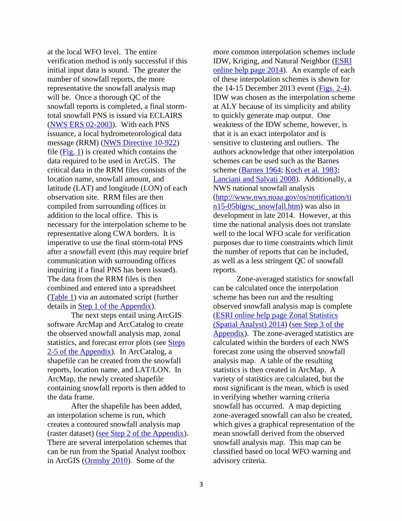
at the local WFO level. The entire

verification method is only successful if this

initial input data is sound. The greater the

number of snowfall reports, the more

representative the snowfall analysis map

will be. Once a thorough QC of the

snowfall reports is completed, a final storm-

total snowfall PNS is issued via ECLAIRS

(NWS ERS 02-2003). With each PNS

issuance, a local hydrometeorological data

message (RRM) (NWS Directive 10-922)

file (Fig. 1) is created which contains the

data required to be used in ArcGIS. The

critical data in the RRM files consists of the

location name, snowfall amount, and

latitude (LAT) and longitude (LON) of each

observation site. RRM files are then

compiled from surrounding offices in

addition to the local office. This is

necessary for the interpolation scheme to be

representative along CWA borders. It is

imperative to use the final storm-total PNS

after a snowfall event (this may require brief

communication with surrounding offices

inquiring if a final PNS has been issued).

The data from the RRM files is then

combined and entered into a spreadsheet

(Table 1) via an automated script (further

details in Step 1 of the Appendix).

The next steps entail using ArcGIS

software ArcMap and ArcCatalog to create

the observed snowfall analysis map, zonal

statistics, and forecast error plots (see Steps

2-5 of the Appendix). In ArcCatalog, a

shapefile can be created from the snowfall

reports, location name, and LAT/LON. In

ArcMap, the newly created shapefile

containing snowfall reports is then added to

the data frame.

After the shapefile has been added,

an interpolation scheme is run, which

creates a contoured snowfall analysis map

(raster dataset) (see Step 2 of the Appendix).

There are several interpolation schemes that

can be run from the Spatial Analyst toolbox

in ArcGIS (Ormsby 2010). Some of the

more common interpolation schemes include

IDW, Kriging, and Natural Neighbor (ESRI

online help page 2014). An example of each

of these interpolation schemes is shown for

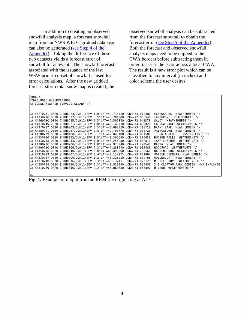
the 14-15 December 2013 event (Figs. 2-4).

IDW was chosen as the interpolation scheme

at ALY because of its simplicity and ability

to quickly generate map output. One

weakness of the IDW scheme, however, is

that it is an exact interpolator and is

sensitive to clustering and outliers. The

authors acknowledge that other interpolation

schemes can be used such as the Barnes

scheme (Barnes 1964; Koch et al. 1983;

Lanciani and Salvati 2008). Additionally, a

NWS national snowfall analysis

(http://www.nws.noaa.gov/os/notification/ti

n15-05bigrsc_snowfall.htm) was also in

development in late 2014. However, at this

time the national analysis does not translate

well to the local WFO scale for verification

purposes due to time constraints which limit

the number of reports that can be included,

as well as a less stringent QC of snowfall

reports.

Zone-averaged statistics for snowfall

can be calculated once the interpolation

scheme has been run and the resulting

observed snowfall analysis map is complete

(ESRI online help page Zonal Statistics

(Spatial Analyst) 2014) (see Step 3 of the

Appendix). The zone-averaged statistics are

calculated within the borders of each NWS

forecast zone using the observed snowfall

analysis map. A table of the resulting

statistics is then created in ArcMap. A

variety of statistics are calculated, but the

most significant is the mean, which is used

in verifying whether warning criteria

snowfall has occurred. A map depicting

zone-averaged snowfall can also be created,

which gives a graphical representation of the

mean snowfall derived from the observed

snowfall analysis map. This map can be

classified based on local WFO warning and

advisory criteria.

4

In addition to creating an observed

snowfall analysis map, a forecast snowfall

map from an NWS WFO’s gridded database

can also be generated (see Step 4 of the

Appendix). Taking the difference of these

two datasets yields a forecast error of

snowfall for an event. The snowfall forecast

associated with the issuance of the last

WSW prior to onset of snowfall is used for

error calculations. After the new gridded

forecast storm total snow map is created, the

observed snowfall analysis can be subtracted

from the forecast snowfall to obtain the

forecast error (see Step 5 of the Appendix).

Both the forecast and observed snowfall

analysis maps need to be clipped to the

CWA borders before subtracting them in

order to assess the error across a local CWA.

The result is a new error plot which can be

classified to any interval (in inches) and

color scheme the user desires.

Fig. 1. Example of output from an RRM file originating at ALY.

5

Table 1. Example of a spreadsheet with relevant data extracted from an RRM file.

6

Fig. 2. Observed snowfall analysis map using IDW interpolation from 14-15 December 2013.

Point values represent actual snowfall observations, while color contours represent interpolated

data.

7

Fig. 3. Observed snowfall analysis map using Kriging interpolation from 14-15 December 2013.

Point values represent actual snowfall observations, while color contours represent interpolated

data.

8

Fig. 4. Observed snowfall analysis map using Natural Neighbor interpolation from 14-15

December 2013. Point values represent actual snowfall observations, while color contours

represent interpolated data.

3. Results

Many of the more significant

snowfall events from the 2013-2014 winter

season are examined, with output from the

gridded verification method shown. The

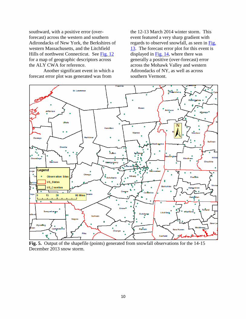
first example is a snowstorm that impacted

the ALY CWA from 14-15 December 2013.

The output of the shapefile generated from

the snowfall observations can be seen in Fig.

5. Figure 2 shows the observed snowfall

analysis map using IDW interpolation,

overlaid with actual snowfall observations

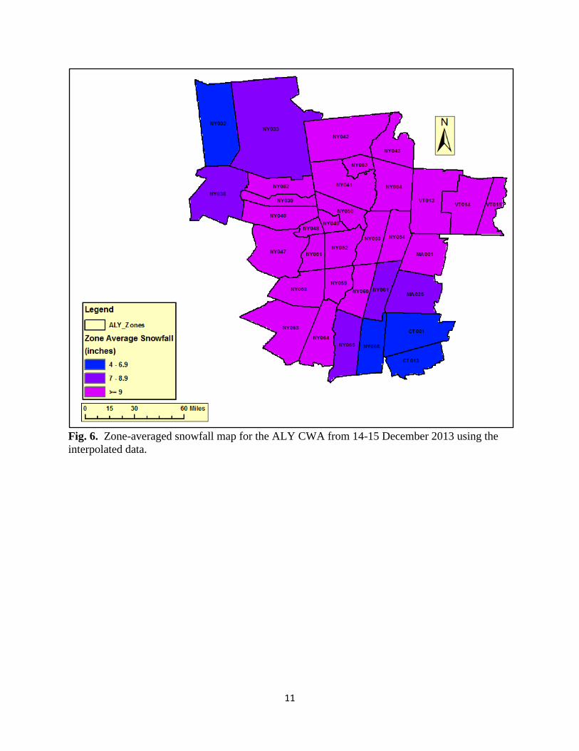
for specific points. A zone-averaged

snowfall map (Fig. 6) displays which ALY

forecast zones reached various snowfall

thresholds corresponding to NWS ALY

advisory and warning criteria (10 to < 18 cm

[4 to < 7 inches], 18 to < 23 cm [7 to < 9

inches], and > 23 cm [> 9 inches]). Lastly,

the zone-averaged statistics table using the

gridded method can be seen in Table 2. The

mean snowfall is used to determine if each

9

forecast zone received warning criteria

snow.

The legacy method of zone-averaged

snowfall consists of summing the snowfall

totals in each zone and dividing by the

number of reports. In comparing the legacy

method to the gridded verification method,

some differences are apparent from the 14-

15 December 2013 event. The mean

snowfall table using the legacy method and

the difference from the gridded method are

also shown in Table 2. For some of the

zones, the difference in zone-averaged

snowfall between the two methods is as

large as 2.5 to 5 cm (1 to 2 inches). An

example of why these differences occurred

could be attributed to a lack of snowfall

reports within a particular zone. With the

legacy method, there may be only one or

two reports in an entire zone. This can yield

a very rough estimate for mean snowfall.

However, the gridded method incorporates

data within the entire forecast zone. This is

possible since the zone-average is computed

using the observed gridded snowfall. This is

a significant advantage of the gridded

method.

Specific differences can be seen by

comparing results for zones NY038

(southern Herkimer County), NY043

(northern Washington County), and NY061

(eastern Columbia County) in Table 2.

There were even two zones in this event,

NY032 (northern Herkimer County) and

CT013 (southern Litchfield County), in

which there were no snowfall reports. In

this situation, the gridded method at least

yielded an approximate value for mean

snowfall even without any reports in the

zone due to deriving data from the observed

snowfall analysis. These interpolated values

can be used for verification to objectively

represent reasonable snowfall

approximation. Using the legacy method

would result in no data for the zone. A

caveat of using the gridded method is when

no snowfall reports exist in a zone it is

possible for data to be misrepresented

depending on the situation, especially if

outliers are present.

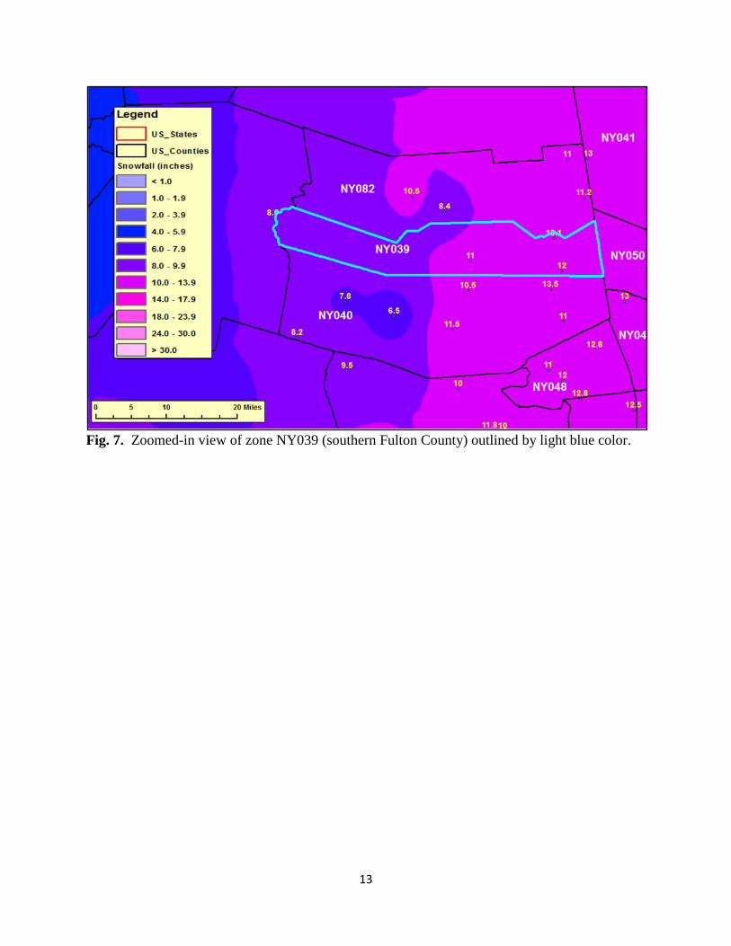
One more example from the 14-15

December 2013 event shows why the

gridded method is more representative. This

is depicted in zone NY039 (southern Fulton

County). Observed snowfall reports were

all clustered in the eastern half of the zone.

Using the legacy method, this resulted in the

mean snowfall for the entire zone being

skewed towards the higher snowfall totals in

the eastern half of the zone. However, when

looking at the observed snowfall analysis

map (Fig. 7) and using the gridded method,

a west to east gradient in the snowfall can

clearly be seen. The gridded method

accounts for this gradient and thus yields a

better representation of the mean snowfall

across the entire zone.

The observed snowfall analysis maps

for the 1-3 January 2014 and 13-14 February

2014 snowstorms are also shown in Figs. 8

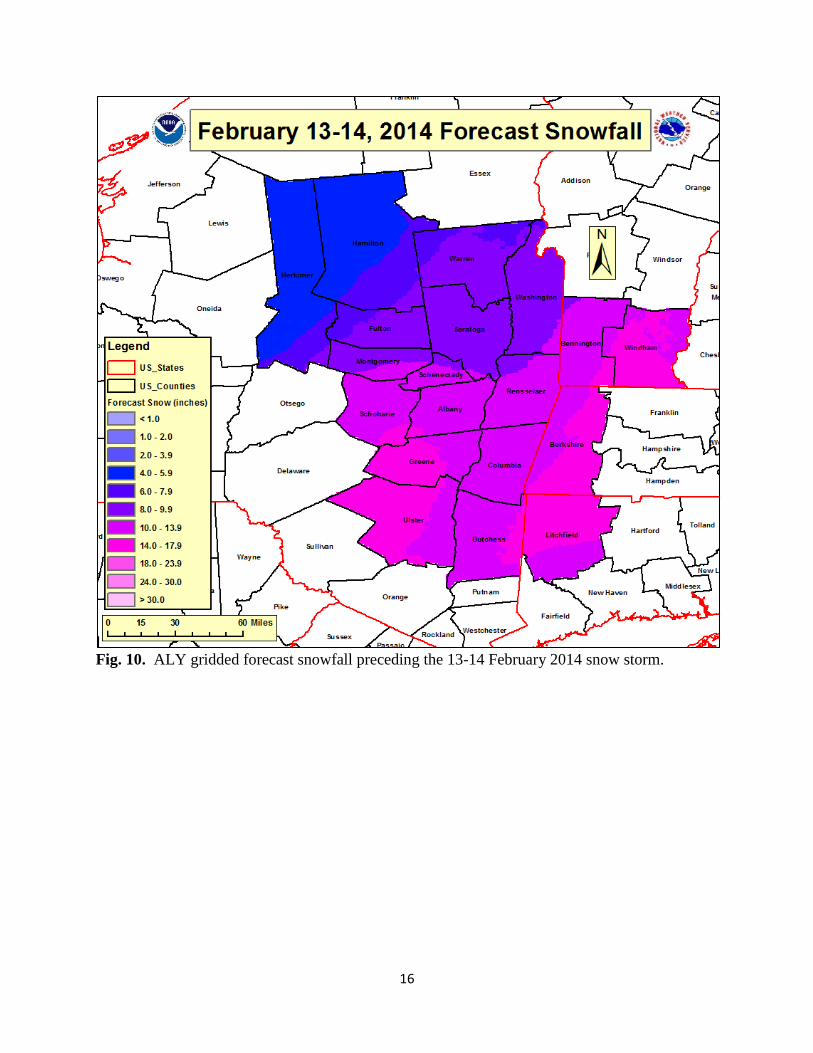
and 9 respectively. For the 13-14 February

2014 event, forecast error plots have been

generated. This is done by comparing the

ALY forecast storm total snow grid

preceding the event (concurrent with WSW

issuance), to the observed snowfall analysis

map. As detailed in the Data and

Methodology section, the observed snowfall

analysis is subtracted from the forecast

snowfall in ArcMap to determine the

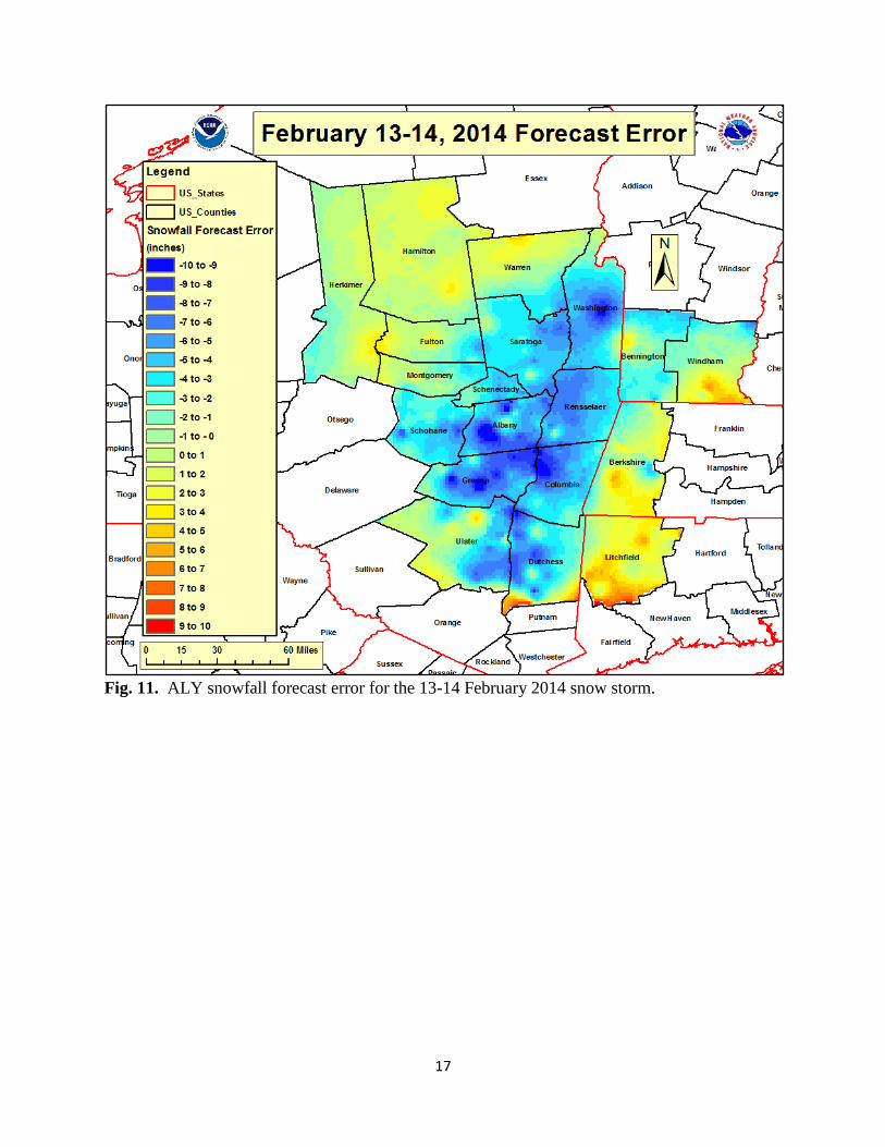
forecast error. Figure 10 shows the ALY

gridded forecast snowfall map preceding

this event. Figure 11 displays the forecast

error for the 13-14 February 2014 event,

with cold colors (negative error)

representing an under-forecast of snowfall

and warm colors (positive error)

representing an over-forecast of snowfall.

The forecast error for this event was

generally negative (under-forecast) across

east central New York from around the

Saratoga region and Capital District

10

southward, with a positive error (over-

forecast) across the western and southern

Adirondacks of New York, the Berkshires of

western Massachusetts, and the Litchfield

Hills of northwest Connecticut. See Fig. 12

for a map of geographic descriptors across

the ALY CWA for reference.

Another significant event in which a

forecast error plot was generated was from

the 12-13 March 2014 winter storm. This

event featured a very sharp gradient with

regards to observed snowfall, as seen in Fig.

13. The forecast error plot for this event is

displayed in Fig. 14, where there was

generally a positive (over-forecast) error

across the Mohawk Valley and western

Adirondacks of NY, as well as across

southern Vermont.

Fig. 5. Output of the shapefile (points) generated from snowfall observations for the 14-15

December 2013 snow storm.

11

Fig. 6. Zone-averaged snowfall map for the ALY CWA from 14-15 December 2013 using the

interpolated data.

12

Table 2. Zone-averaged statistics table displaying mean snowfall from 14-15 December 2013

comparing gridded and legacy verification methods.

13

Fig. 7. Zoomed-in view of zone NY039 (southern Fulton County) outlined by light blue color.

14

Fig. 8. Observed snowfall analysis map from 1-3 January 2014 overlaid with snowfall

observations. Point values represent actual snowfall observations, while color contours represent

interpolated data.

15

Fig. 9. Observed snowfall analysis map from 13-14 February 2014 overlaid with snowfall

observations. Point values represent actual snowfall observations, while color contours represent

interpolated data.

16

Fig. 10. ALY gridded forecast snowfall preceding the 13-14 February 2014 snow storm.

17

Fig. 11. ALY snowfall forecast error for the 13-14 February 2014 snow storm.

18

Fig. 12. Map of primary geographic descriptors for the ALY CWA.

19

Fig. 13. Observed snowfall analysis map from 12-13 March 2014 overlaid with snowfall

observations. Point values represent actual snowfall observations, while color contours represent

interpolated data.

20

Fig. 14. ALY snowfall forecast error for the 12-13 March 2014 winter storm.

4. Discussion

The WFO ALY staff endorsed the

gridded snowfall verification method to

become official before the 2013-2014 winter

season. After a full season of using this new

verification scheme, the ALY staff has

provided positive feedback. As shown in

the Results section, this method improves

upon the legacy practice of summing

snowfall reports and dividing by the number

of reports for each forecast zone. Creating

gridded observed snowfall maps yields a

more representative depiction of snowfall

spatially across a CWA and aides in

conducting zone-based verification in a

more thorough manner. Other NWS offices

can adopt this gridded snowfall verification

while still maintaining NWS zone-based

verification.

For NWS offices that would like to

implement this gridded snowfall verification

method, job sheets (found in the Appendix)

have been constructed detailing each step of

the process, from creating the initial

shapefile based on snowfall reports, to

generating observed snowfall analysis maps

and generating forecast error plots for

snowfall. Any NWS office that has access

to GIS software can adopt this method.

Another advantage of generating

gridded snowfall maps is that they can be

21

easily displayed in a variety of graphical

formats. Any GIS-based format can be

generated as output such as KMZ, KML

files (Google Keyhole Markup Language

2014), as well as common digital image

formats. The graphics can be used for

Decision Support Services dissemination, as

well as in post-mortem reviews of snow

events. The forecast ranges and color scales

can easily be adapted to match the latest

standardized NWS Eastern Region forecast

snowfall ranges.

In addition to computing snowfall

verification for storm-total snowfall, 24-

hour snowfall can also be verified. This can

be accomplished by summing 6-hour

snowfall grids from the NWS gridded

forecast database over a 24-hour period,

typically ending 1200 UTC. This is when

many trained weather spotters regularly

report precipitation to NWS WFO’s.

Additional time steps can also be analyzed

based on user preference.

Internally, forecast error plots of

snowfall events can be compiled over entire

winter seasons to compute potential positive

or negative biases that may exist

consistently over certain areas. This would

be particularly beneficial to NWS

forecasters in potentially improving snowfall

forecasts. Biases for events could be

stratified into different flow regimes, as well

as storm tracks. At a base level, it would be

valuable for NWS WFO’s to simply start

looking at forecast biases since it is difficult

to improve forecasting snowfall without

knowing spatially how forecasts verify.

This gridded verification method can enable

NWS WFO’s to start examining potential

forecast biases relatively quickly and easily.

5. Future Work

Many of the stages of the gridded

snowfall verification in the job sheets (see

Appendix) created at WFO ALY must

currently be performed manually by a user.

This can be a lengthy process, especially to

those who have limited experience using

GIS software. Therefore, automating most

of the verification process would be

advantageous. Automation will be a crucial

step going forward in making this method

more accessible to a wider audience. The

authors plan to develop automation

techniques for this gridded verification

method.

Improvements in the interpolation

scheme for snowfall analysis will also be

attempted by exploring more intensive

interpolation schemes, such as the Barnes

objective analysis (Barnes 1964; Koch et al.

1983; Lanciani and Salvati 2008) in the

future. The NWS national snowfall analysis

currently in development at the time of this

writing, utilizes a version of the Barnes

interpolation scheme. Improving the

interpolation for snowfall analysis will lead

to more accurate representation of snowfall

spatially and by extension, zone-based

verification and error plots.

Computing forecast biases for

snowfall is just beginning to tap the

potential for using statistics based on

gridded maps. More advanced statistics can

eventually be developed for snowfall. In

addition, this verification method may

potentially be used for other variables such

as rainfall, temperature, dewpoint, and wind

speed, although this still has to be evaluated.

22

Acknowledgements

The authors would like to thank

Conor Lahiff from NWS Burlington, VT, for

assistance in obtaining information for

converting a NetCDF file to a shapefile.

The authors would also like to acknowledge

Luigi Meccariello from NWS Albany, NY,

for assisting in creating observed snowfall

analysis maps during the 2013-2014 winter

season. The authors also thank John

Quinlan from NWS Albany, NY, for

providing conceptual ideas for computing

zone-averaged statistics. Finally, the

authors would like to acknowledge Warren

Snyder from NWS Albany, NY, and Brian

Miretzky from NWS Eastern Region

Headquarters, Scientific Services Division,

for reviewing this paper.

References

Barnes, S. L., 1964: A technique for

maximizing details in numerical weather

map analysis. J. Appl. Meteor., 3, 396–409.

ESRI online help page, cited. 2014: ArcGIS.

[Available online at:

http://help.arcgis.com/en/arcgisdesktop/10.0

/help/index.html]

ESRI online help page IDW (Spatial

Analyst), cited. 2014: ArcGIS. [Available

online at:

http://help.arcgis.com/en/arcgisdesktop/10.0

/help/index.html#//009z0000006m000000.ht

m]

ESRI online help page Zonal Statistics

(Spatial Analyst), cited. 2014: ArcGIS.

[Available online at:

http://help.arcgis.com/en/arcgisdesktop/10.0

/help/index.html#//009z000000w7000000.ht

m]

Google Keyhole Markup Language, cited.

2014. [Available online at:

https://developers.google.com/kml/documen

tation/mapsSupport]

Koch, S. E., desJardins, M., Kocin, P.J.,

1983: An interactive Barnes objective map

analysis scheme for use with satellite and

conventional data. J. Climate Appl. Meteor.,

22, 1487–1503.

Lanciani, A., and Salvati, M., 2008: Spatial

interpolation of surface weather

observations in Alpine meteorological

services. FORALPS Technical Report, 2.

Università degli Studi di Trento,

Dipartimento di Ingegneria Civile e

Ambientale, Trento, Italy, 40 pp.

NOAA/NWS, Cited 2014: NWS Directives

10-201 National Digital Forecast Database

and Local Database Description and

Specifications [Available online at:

http://www.nws.noaa.gov/directives/sym/pd

01002001curr.pdf]

NOAA/NWS, Cited 2014: NWS Directives

10-507 Public Geographic Areas of

Responsibility. [Available online at:

http://www.nws.noaa.gov/directives/sym/pd

01005007curr.pdf]

NOAA/NWS, Cited 2014: NWS Directives

10-513 WFO Winter Weather Products

Specification. [Available online at:

http://www.nws.noaa.gov/directives/sym/pd

01005013curr.pdf]

NOAA/NWS, Cited 2014: NWS Eastern

Region Supplement 02-2003 (subset of

NWS Directive 10-513). [Available online

at:

http://www.nws.noaa.gov/directives/sym/pd

01005013curr.pdf]

23

NOAA/NWS, Cited 2014: NWS Directives

10-922 Weather Forecast Office Hydrologic

Products Specification: [Available online at

http://www.nws.noaa.gov/directives/sym/pd

01009022curr.pdf]

Ormsby, T. J., et al., 2010: Getting to know

ArcGIS desktop. 2nd Edition. Esri Press,

584 pp.

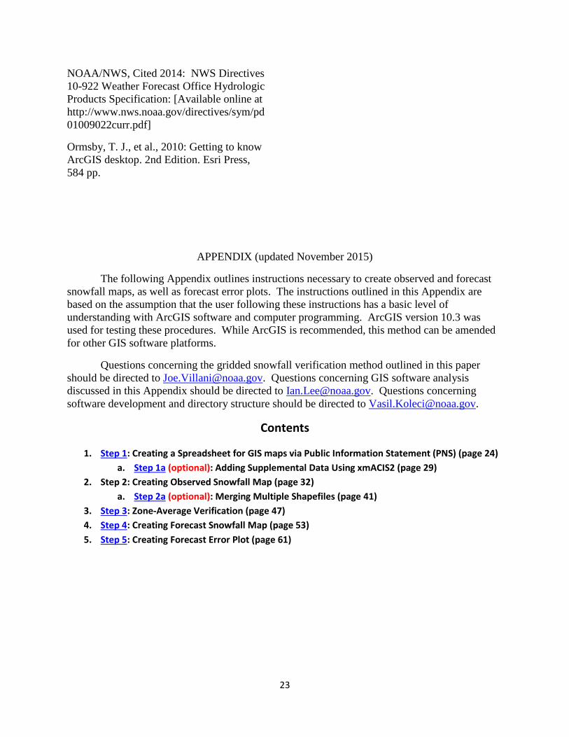
APPENDIX (updated November 2015)

The following Appendix outlines instructions necessary to create observed and forecast

snowfall maps, as well as forecast error plots. The instructions outlined in this Appendix are

based on the assumption that the user following these instructions has a basic level of

understanding with ArcGIS software and computer programming. ArcGIS version 10.3 was

used for testing these procedures. While ArcGIS is recommended, this method can be amended

for other GIS software platforms.

Questions concerning the gridded snowfall verification method outlined in this paper

should be directed to Joe.Villani@noaa.gov. Questions concerning GIS software analysis

discussed in this Appendix should be directed to Ian.Lee@noaa.gov. Questions concerning

software development and directory structure should be directed to Vasil.Koleci@noaa.gov.

Contents

1. Step 1: Creating a Spreadsheet for GIS maps via Public Information Statement (PNS) (page 24)

a. Step 1a (optional): Adding Supplemental Data Using xmACIS2 (page 29)

2. Step 2: Creating Observed Snowfall Map (page 32)

a. Step 2a (optional): Merging Multiple Shapefiles (page 41)

3. Step 3: Zone-Average Verification (page 47)

4. Step 4: Creating Forecast Snowfall Map (page 53)

5. Step 5: Creating Forecast Error Plot (page 61)

24

Step 1: Creating a Spreadsheet for GIS Maps via PNS

This section outlines the instructions necessary to create Microsoft Excel .xls spreadsheets containing

snowfall data from PNS files. This spreadsheet is generated off the final storm total PNS after an event

occurs. Careful QC must be done before issuing the final storm total PNS.

*To obtain the Python program (read_pns.py) and AWIPS directory structure needed for this section,

send an email request to Vasil.Koleci@noaa.gov

1. In an AWIPS text workstation, open up a text window

2. Call up your office’s most recent PNS file after an event, along with the PNS files from your

surrounding offices (dependent upon surrounding office’s IDs)

a. Make sure each PNS file is recent and matches the final PNS you wish to include in the

spreadsheet. It is imperative to use the final storm total PNS after an event (this may

require brief communication with surrounding offices inquiring if a final PNS has been

issued)

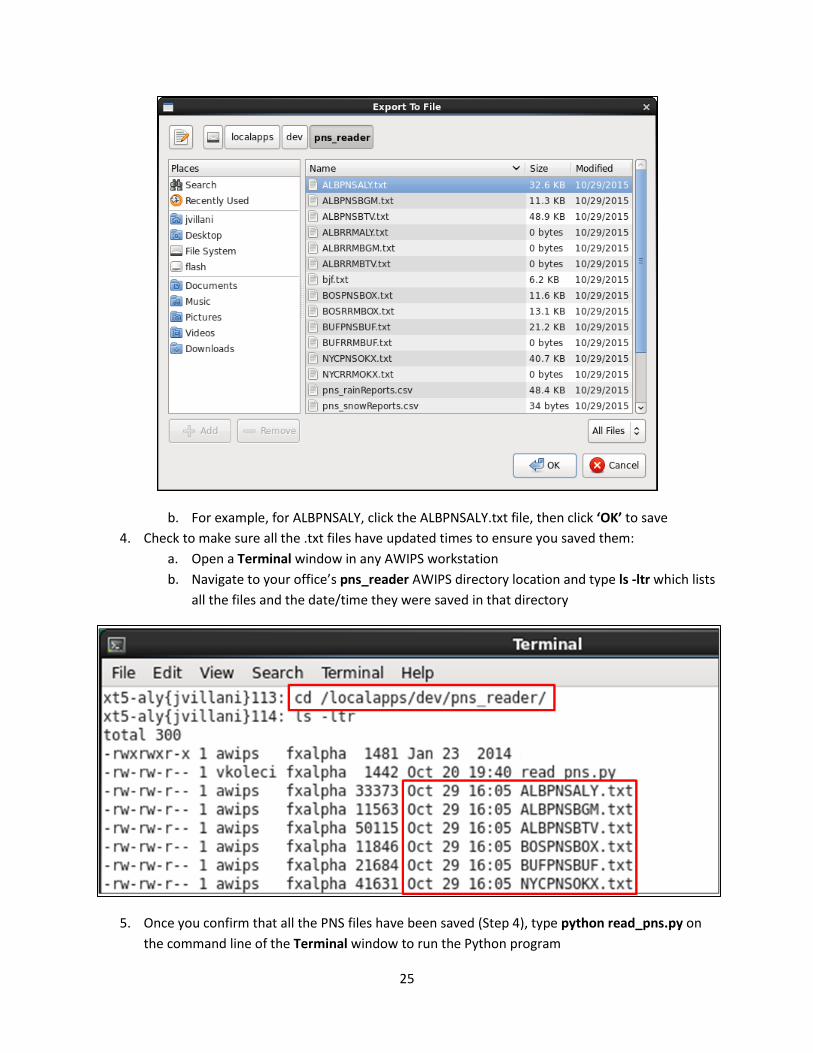
3. Save each PNS file by clicking FileExport to Filethen navigate to the directory where the

Python program is stored via the ‘Directories’ section of the Export to File window

a. In the ‘Files’ section of the text window, click on the .txt file that matches each specific

PNS you are saving and click OK to save the file (this overwrites the old file)

25

b. For example, for ALBPNSALY, click the ALBPNSALY.txt file, then click ‘OK’ to save

4. Check to make sure all the .txt files have updated times to ensure you saved them:

a. Open a Terminal window in any AWIPS workstation

b. Navigate to your office’s pns_reader AWIPS directory location and type ls -ltr which lists

all the files and the date/time they were saved in that directory

5. Once you confirm that all the PNS files have been saved (Step 4), type python read_pns.py on

the command line of the Terminal window to run the Python program

26

a. Running this program will compile all of the PNS files into a single .csv file

b. The name of the newly created .csv file will be pns_snowReports.csv

i. This program also creates a rainfall .csv file as well (pns_rainReports.csv)

6. Check to make sure the pns_snowReports.csv file has updated to ensure it was saved:

a. Make sure you are still in your office’s pns_reader AWIPS directory and type ls -ltr and

check the time of the pns_snowReports.csv file to make sure it was saved

7. Send the newly created pns_snowReports .csv file to the PC using your office’s local method of

transferring AWIPS files to a PC

a. The pns_snowReports.csv file will appear in the specified PC directory that your office

has already set up

8. Open the pns_snowReports.csv file using Microsoft Excel and save the file with a .xls extension

a. *IMPORTANT TO PERFORM THE FOLLOWING QC STEPS BEFORE FINAL SAVE* (QC must

be performed to ensure that the most accurate GIS map is created)

i. Check for and delete bad lat/lon pairs (ex. 99.99, 999, or any combo of 9’s)

ii. Delete any snowfall reports of Trace (T) - this yields errors in the interpolation

iii. If headers at the top of the spreadsheet have not been created, create the

following headers: Location, Snowfall, Source, Lat, Lon

27

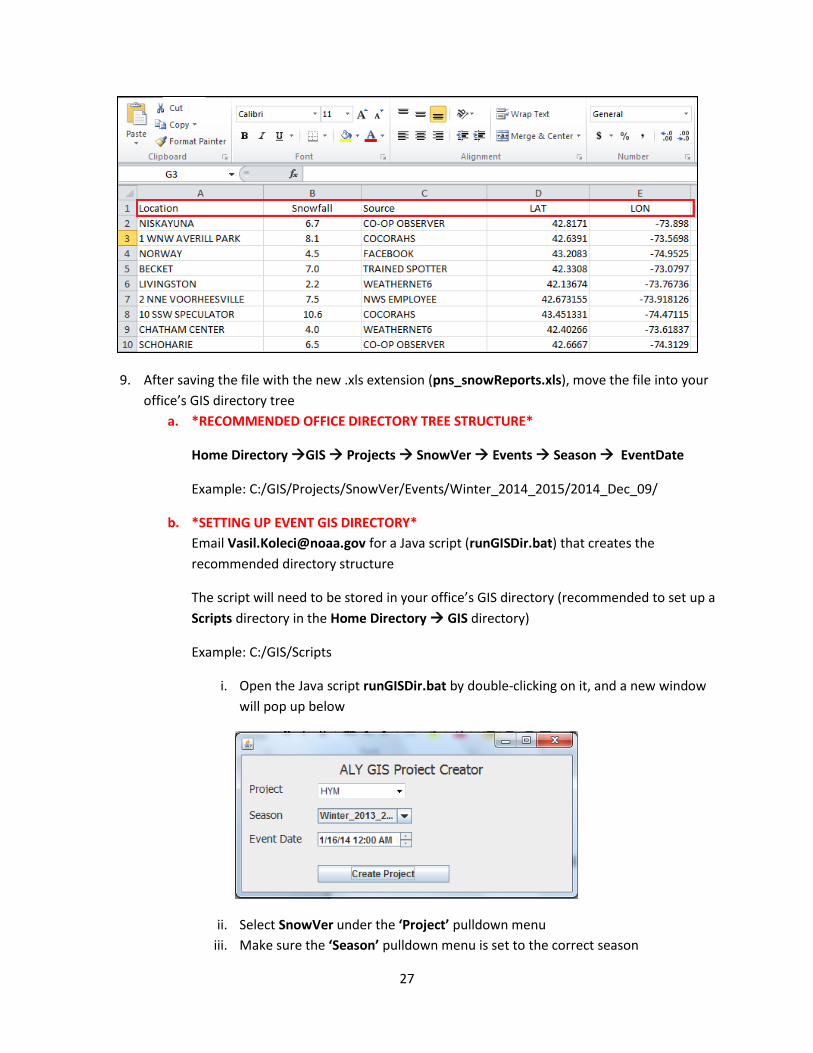
9. After saving the file with the new .xls extension (pns_snowReports.xls), move the file into your

office’s GIS directory tree

a. *RECOMMENDED OFFICE DIRECTORY TREE STRUCTURE*

Home Directory GIS Projects SnowVer Events Season EventDate

Example: C:/GIS/Projects/SnowVer/Events/Winter_2014_2015/2014_Dec_09/

b. *SETTING UP EVENT GIS DIRECTORY*

Email Vasil.Koleci@noaa.gov for a Java script (runGISDir.bat) that creates the

recommended directory structure

The script will need to be stored in your office’s GIS directory (recommended to set up a

Scripts directory in the Home Directory GIS directory)

Example: C:/GIS/Scripts

i. Open the Java script runGISDir.bat by double-clicking on it, and a new window

will pop up below

ii. Select SnowVer under the ‘Project’ pulldown menu

iii. Make sure the ‘Season’ pulldown menu is set to the correct season

28

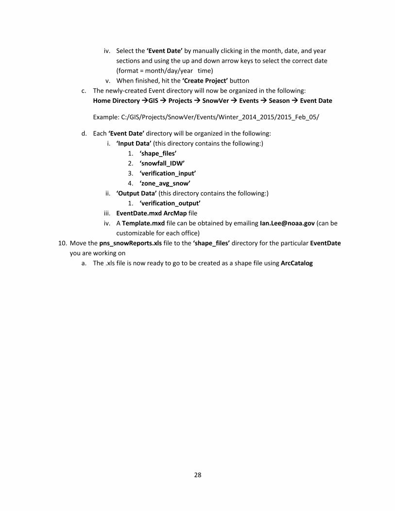
iv. Select the ‘Event Date’ by manually clicking in the month, date, and year

sections and using the up and down arrow keys to select the correct date

(format = month/day/year time)

v. When finished, hit the ‘Create Project’ button

c. The newly-created Event directory will now be organized in the following:

Home Directory GIS Projects SnowVer Events Season Event Date

Example: C:/GIS/Projects/SnowVer/Events/Winter_2014_2015/2015_Feb_05/

d. Each ‘Event Date’ directory will be organized in the following:

i. ‘Input Data’ (this directory contains the following:)

1. ‘shape_files’

2. ‘snowfall_IDW’

3. ‘verification_input’

4. ‘zone_avg_snow’

ii. ‘Output Data’ (this directory contains the following:)

1. ‘verification_output’

iii. EventDate.mxd ArcMap file

iv. A Template.mxd file can be obtained by emailing Ian.Lee@noaa.gov (can be

customizable for each office)

10. Move the pns_snowReports.xls file to the ‘shape_files’ directory for the particular EventDate

you are working on

a. The .xls file is now ready to go to be created as a shape file using ArcCatalog

29

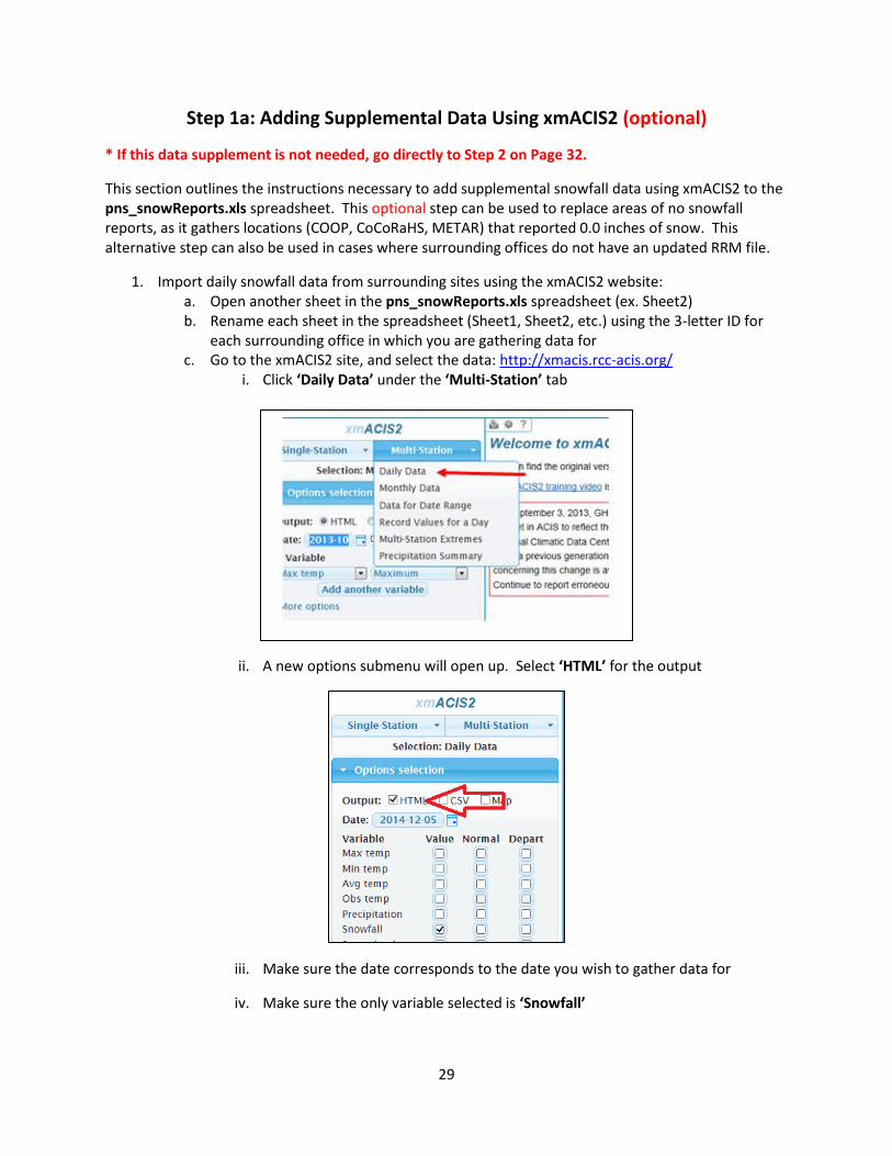
Step 1a: Adding Supplemental Data Using xmACIS2 (optional)

* If this data supplement is not needed, go directly to Step 2 on Page 32.

This section outlines the instructions necessary to add supplemental snowfall data using xmACIS2 to the pns_snowReports.xls spreadsheet. This optional step can be used to replace areas of no snowfall reports, as it gathers locations (COOP, CoCoRaHS, METAR) that reported 0.0 inches of snow. This alternative step can also be used in cases where surrounding offices do not have an updated RRM file.

1. Import daily snowfall data from surrounding sites using the xmACIS2 website: a. Open another sheet in the pns_snowReports.xls spreadsheet (ex. Sheet2) b. Rename each sheet in the spreadsheet (Sheet1, Sheet2, etc.) using the 3-letter ID for

each surrounding office in which you are gathering data for c. Go to the xmACIS2 site, and select the data: http://xmacis.rcc-acis.org/

i. Click ‘Daily Data’ under the ‘Multi-Station’ tab

ii. A new options submenu will open up. Select ‘HTML’ for the output

iii. Make sure the date corresponds to the date you wish to gather data for

iv. Make sure the only variable selected is ‘Snowfall’

30

v. Click to open up the ‘More Options’ submenu and make sure that ‘Include station coordinates’ is the only checked box

vi. Open the ‘Station Selection’ submenu and select the appropriate forecast office county warning area (CWA), then click ‘Go’

vii. A new HTML spreadsheet will pop up to the right. Before copying the data, QC it and make note of any erroneous data or M’s that will need to be deleted from

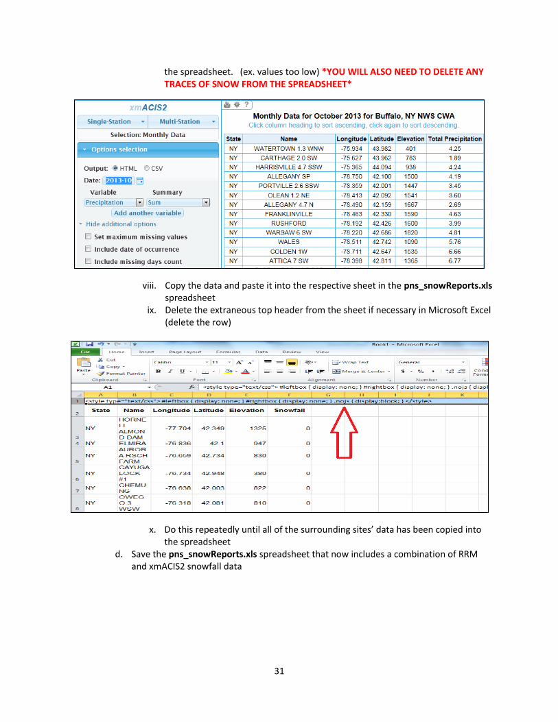
31

the spreadsheet. (ex. values too low) *YOU WILL ALSO NEED TO DELETE ANY TRACES OF SNOW FROM THE SPREADSHEET*

viii. Copy the data and paste it into the respective sheet in the pns_snowReports.xls spreadsheet

ix. Delete the extraneous top header from the sheet if necessary in Microsoft Excel (delete the row)

x. Do this repeatedly until all of the surrounding sites’ data has been copied into the spreadsheet

d. Save the pns_snowReports.xls spreadsheet that now includes a combination of RRM and xmACIS2 snowfall data

32

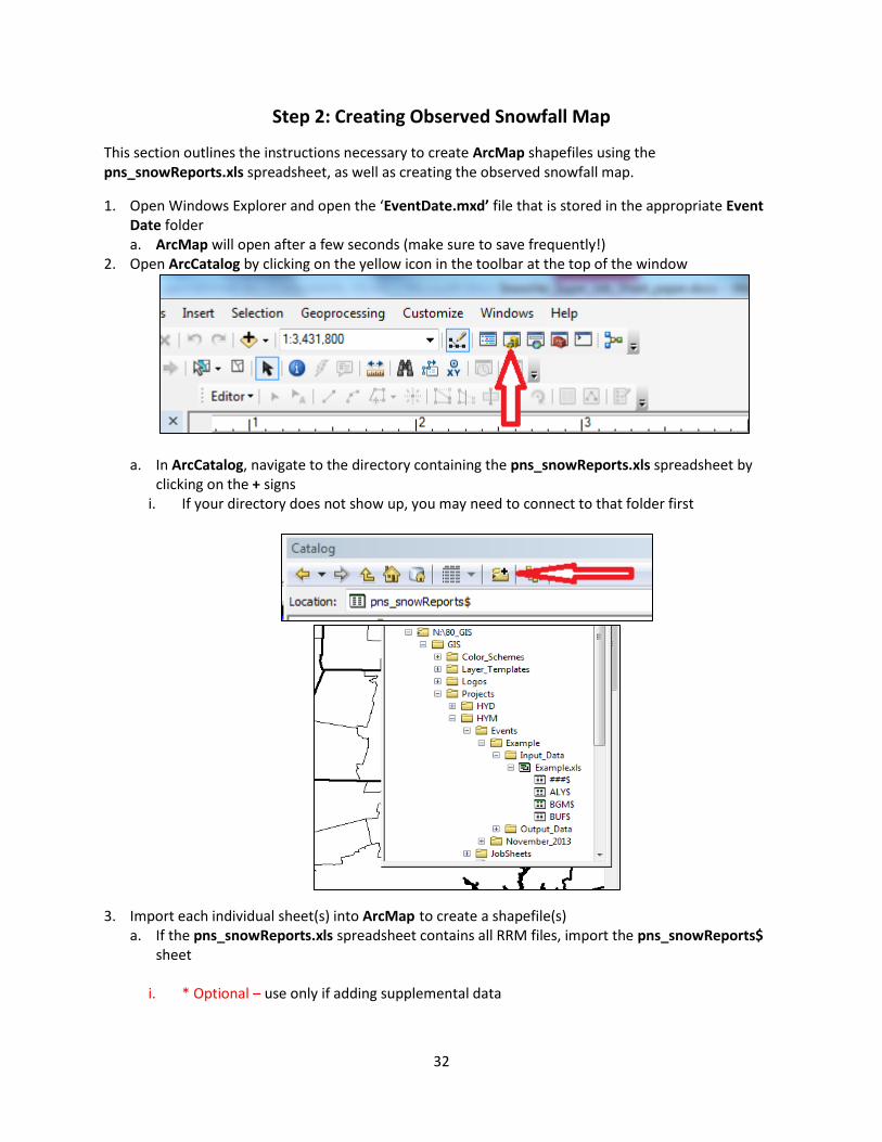
Step 2: Creating Observed Snowfall Map

This section outlines the instructions necessary to create ArcMap shapefiles using the pns_snowReports.xls spreadsheet, as well as creating the observed snowfall map.

1. Open Windows Explorer and open the ‘EventDate.mxd’ file that is stored in the appropriate Event Date folder a. ArcMap will open after a few seconds (make sure to save frequently!)

2. Open ArcCatalog by clicking on the yellow icon in the toolbar at the top of the window

a. In ArcCatalog, navigate to the directory containing the pns_snowReports.xls spreadsheet by

clicking on the + signs i. If your directory does not show up, you may need to connect to that folder first

3. Import each individual sheet(s) into ArcMap to create a shapefile(s) a. If the pns_snowReports.xls spreadsheet contains all RRM files, import the pns_snowReports$

sheet

i. * Optional – use only if adding supplemental data

33

(a) (If the spreadsheet contains a combination of RRM files and xmACIS2 data, import each individual sheet )

(b) Example: Two sheets from a combo of RRM/xmACIS2 data from ALY and BGM (Binghamton, NY)

(c) First sheet imported would be pns_snowReports$ (ALY data) (d) Second sheet imported would be BGM$ (would containing BGM xmACIS2 snowfall

data)

b. Set up the shapefile parameters i. Right-click on each sheet(s), and scroll down to ‘Create Feature Class’ and hover over it until

‘From XY Table’ pops up

c. Click ‘From XY Table’ to open up a new window i. For the ‘X Field’ set it to ‘Lon’ (or ‘Longitude’ if using xmACIS2 data) and set the ‘Y Field’

to ‘Lat’ (or ‘Latitude’ if using xmACIS2 data). Set the ‘Z Field’ to ‘Snowfall’. Set the ‘Output’ to the ‘shape_files’ directory in the respective EventDate directory by clicking on the folder icon and rename each sheet(s) to ‘snowfall.shp’

ii. If using multiple sheets, rename each additional sheet as snowfall1.shp, snowfall2.shp,

etc. iii. Set the ‘Coordinate System of Input Coordinates’ to ‘NAD 1983’ under ‘Geographic

Coordinate Systems’ ‘North America’

34

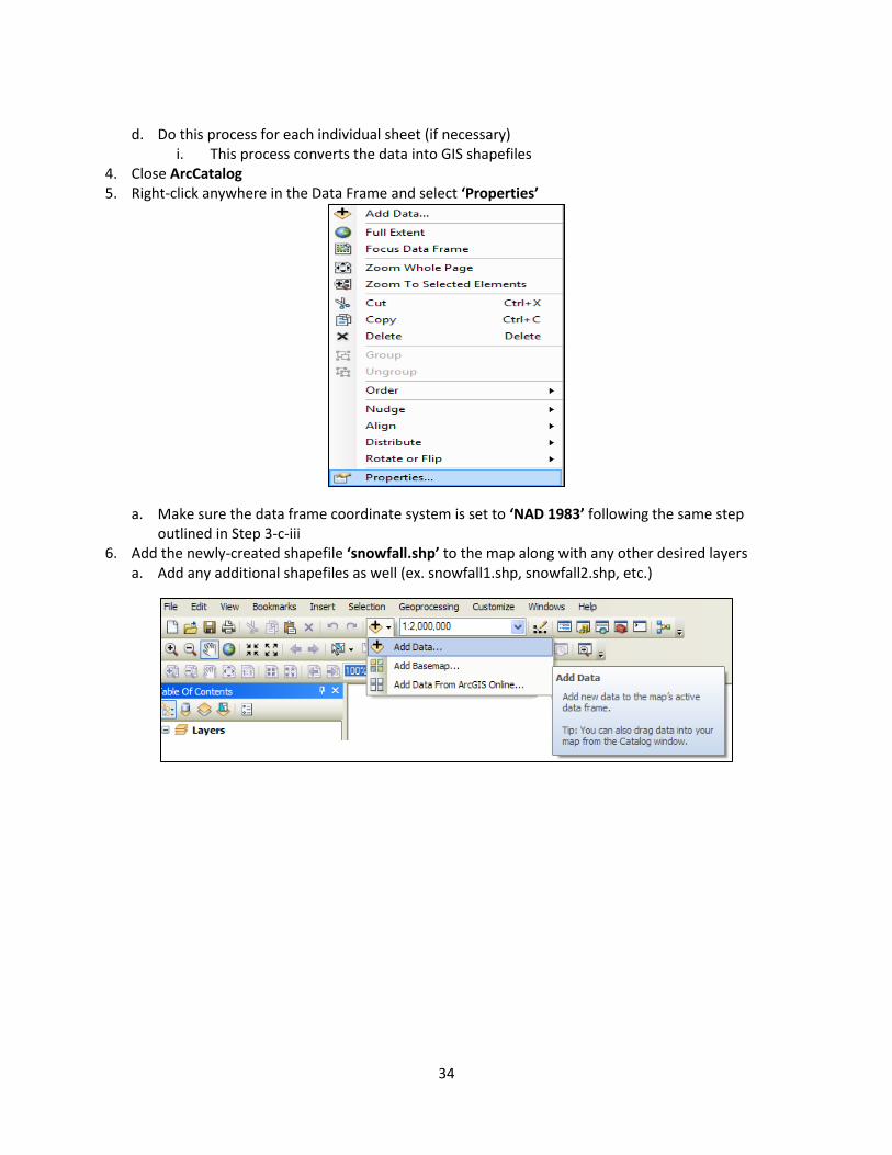
d. Do this process for each individual sheet (if necessary)

i. This process converts the data into GIS shapefiles 4. Close ArcCatalog 5. Right-click anywhere in the Data Frame and select ‘Properties’

a. Make sure the data frame coordinate system is set to ‘NAD 1983’ following the same step outlined in Step 3-c-iii

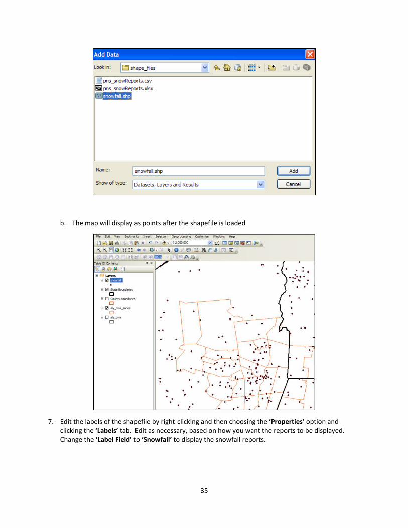
6. Add the newly-created shapefile ‘snowfall.shp’ to the map along with any other desired layers a. Add any additional shapefiles as well (ex. snowfall1.shp, snowfall2.shp, etc.)

35

b. The map will display as points after the shapefile is loaded

7. Edit the labels of the shapefile by right-clicking and then choosing the ‘Properties’ option and clicking the ‘Labels’ tab. Edit as necessary, based on how you want the reports to be displayed. Change the ‘Label Field’ to ‘Snowfall’ to display the snowfall reports.

36

8. After changing the label field, the map will display the snowfall reports after clicking ‘OK’

37

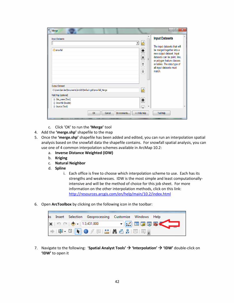
9. Once the shapefile has been added and edited, you can run an interpolation spatial analysis based on the snowfall data the shapefile contains. For snowfall spatial analysis, you can use one of 4 common interpolation schemes available in ArcMap, version 10.2: a. Inverse Distance Weighted (IDW) b. Kriging c. Natural Neighbor d. Spline

i. Each office is free to choose which interpolation scheme to use. Each has its strengths and weaknesses. IDW is the most simple and least computationally-intensive. This job sheet will go through the IDW interpolation method. For more information on the other interpolation methods, click on this link: http://resources.arcgis.com/en/help/main/10.2/index.html

10. Open ArcToolbox by clicking on the following icon in the toolbar:

11. Navigate to the following: ‘Spatial Analyst Tools’ ‘Interpolation’ ‘IDW’ and double-click on ‘IDW’ to open it

38

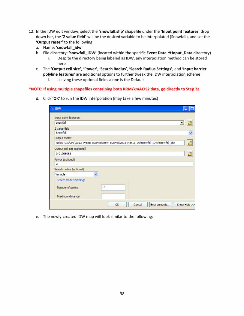
12. In the IDW edit window, select the ‘snowfall.shp’ shapefile under the ‘Input point features’ drop down bar, the ‘Z value field’ will be the desired variable to be interpolated (Snowfall), and set the ‘Output raster’ to the following: a. Name: ‘snowfall_idw’ b. File directory: ‘snowfall_IDW’ (located within the specific Event Date Input_Data directory)

i. Despite the directory being labeled as IDW, any interpolation method can be stored here

c. The ‘Output cell size’, ‘Power’, ‘Search Radius’, ‘Search Radius Settings’, and ‘Input barrier polyline features’ are additional options to further tweak the IDW interpolation scheme

i. Leaving these optional fields alone is the Default

*NOTE: If using multiple shapefiles containing both RRM/xmACIS2 data, go directly to Step 2a

d. Click ‘OK’ to run the IDW interpolation (may take a few minutes)

e. The newly-created IDW map will look similar to the following:

39

13. After the IDW (or other interpolation method) map has been created, the values will need to be reclassified to match the NWS Eastern Region forecast snowfall graphics. a. Right-click on the interpolated raster layer and click on ‘Properties’ to open the ‘Layer

Properties’ popup window b. Click on the ‘Symbology’ tab (if not already selected) c. Make sure it is set to ‘Classified’ (left side of the popup window)

d. Click the ‘Open’ button to import the ‘snow_color_updated.lyr’ color scheme from the ‘Import Symbology’ popup window (navigate to the directory where the color scheme is saved) *RECOMMENDED OFFICE DIRECTORY TREE STRUCTURE FOR COLOR SCHEMES*

Home Directory GIS Color_Schemes Example: C:/GIS/Color_Schemes/

*To obtain the ‘snow_color_updated.lyr’ color scheme, email Ian.Lee@noaa.gov

40

e. After clicking ‘OK’ the ‘snow_color_updated.lyr’ color scheme will update and should resemble the legend below (this scheme is already pre-formatted and does not require any further editing):

f. Click ‘OK’ again to apply the color scheme changes to the interpolated map

14. Make any final changes to the map as necessary (exs. legend, title, scale, disclaimer, north arrow,

adding additional layers, etc.) 15. ‘Print Screen’ and crop and save the image using Paint as a .png file

a. Name the image using a common nomenclature (ex. Observed_Snowfall_121214.png) b. Save the image in the specific Event Date Output_Data verification_output directory

41

Step 2a: Merging Multiple Shapefiles (optional)

*Skip this step if only using one shapefile where observations are solely from PNS/RRM and go directly to Step 3 on Page 26.

This section outlines the instructions necessary to merge multiple ArcMap shapefiles using a pns_snowReports.xls spreadsheet that contains RRM and xmACIS2 data, as well as creating the observed snowfall map.

1. Merge all the imported shapefiles into one shapefile using the ‘Merge’ tool a. Using multiple shapefiles such as snowfall.shp, snowfall1.shp, snowfall2.shp, etc.

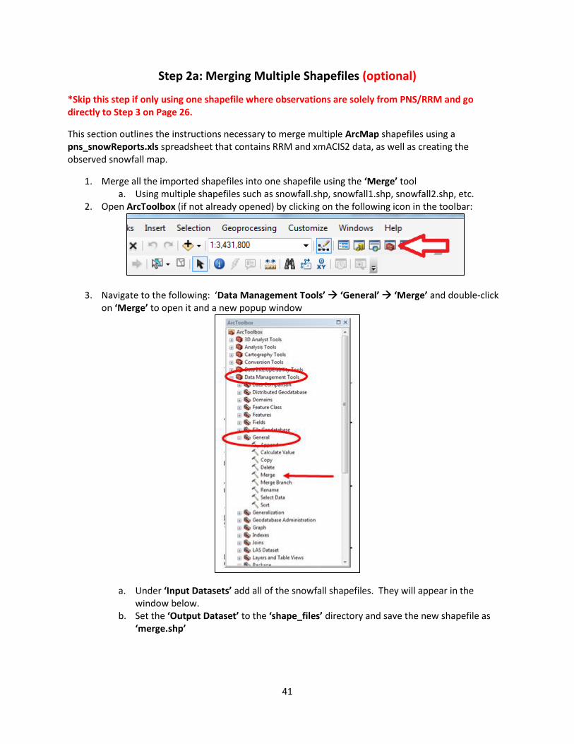
2. Open ArcToolbox (if not already opened) by clicking on the following icon in the toolbar:

3. Navigate to the following: ‘Data Management Tools’ ‘General’ ‘Merge’ and double-click

on ‘Merge’ to open it and a new popup window

a. Under ‘Input Datasets’ add all of the snowfall shapefiles. They will appear in the window below.

b. Set the ‘Output Dataset’ to the ‘shape_files’ directory and save the new shapefile as ‘merge.shp’

42

c. Click ‘OK’ to run the ‘Merge’ tool

4. Add the ‘merge.shp’ shapefile to the map 5. Once the ‘merge.shp’ shapefile has been added and edited, you can run an interpolation spatial

analysis based on the snowfall data the shapefile contains. For snowfall spatial analysis, you can use one of 4 common interpolation schemes available in ArcMap 10.2:

a. Inverse Distance Weighted (IDW) b. Kriging c. Natural Neighbor d. Spline

i. Each office is free to choose which interpolation scheme to use. Each has its strengths and weaknesses. IDW is the most simple and least computationally-intensive and will be the method of choice for this job sheet. For more information on the other interpolation methods, click on this link: http://resources.arcgis.com/en/help/main/10.2/index.html

6. Open ArcToolbox by clicking on the following icon in the toolbar:

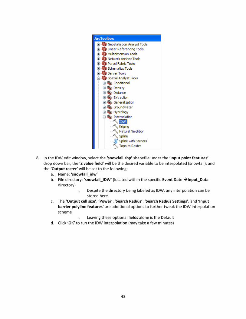
7. Navigate to the following: ‘Spatial Analyst Tools’ ‘Interpolation’ ‘IDW’ double-click on

‘IDW’ to open it

43

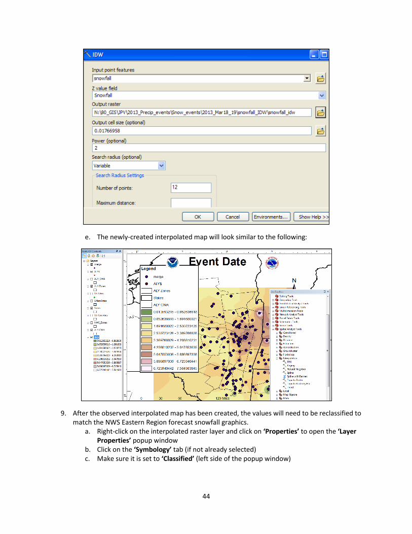
8. In the IDW edit window, select the ‘snowfall.shp’ shapefile under the ‘Input point features’

drop down bar, the ‘Z value field’ will be the desired variable to be interpolated (snowfall), and the ‘Output raster’ will be set to the following:

a. Name: ‘snowfall_idw’ b. File directory: ‘snowfall_IDW’ (located within the specific Event Date Input_Data

directory) i. Despite the directory being labeled as IDW, any interpolation can be

stored here c. The ‘Output cell size’, ‘Power’, ‘Search Radius’, ‘Search Radius Settings’, and ‘Input

barrier polyline features’ are additional options to further tweak the IDW interpolation scheme

i. Leaving these optional fields alone is the Default d. Click ‘OK’ to run the IDW interpolation (may take a few minutes)

44

e. The newly-created interpolated map will look similar to the following:

9. After the observed interpolated map has been created, the values will need to be reclassified to match the NWS Eastern Region forecast snowfall graphics.

a. Right-click on the interpolated raster layer and click on ‘Properties’ to open the ‘Layer Properties’ popup window

b. Click on the ‘Symbology’ tab (if not already selected) c. Make sure it is set to ‘Classified’ (left side of the popup window)

45

d. Click the ‘Open’ button to import the ‘snow_color_updated.lyr’ color scheme from the ‘Import Symbology’ popup window (navigate to the directory where the color scheme is saved)

i. *RECOMMENDED OFFICE DIRECTORY TREE STRUCTURE FOR COLOR SCHEMES*

Home Directory GIS Color_Schemes

Example: C:/GIS/Color_Schemes/

*To obtain the ‘snow_color_updated.lyr’ color scheme, email Ian.Lee@noaa.gov

46

e. After clicking ‘OK’ the ‘snow_color_updated.lyr’ color scheme will update and should resemble the legend below (this scheme is already pre-formatted and does not require any further editing):

f. Click ‘OK’ again to apply the color scheme changes to the interpolated map 10. Make any final changes to the map as necessary (exs. legend, title, scale, disclaimer, north

arrow, adding additional layers, etc.) 11. ‘Print Screen’ and crop and save the image using Paint as a .png file

a. Name the image using a common nomenclature (ex. Observed_Snowfall_121214.png) b. Save the image in the specific Event Date Output_Data verification_output

directory

47

Step 3: Zone-Average Verification

This section outlines the instructions necessary to perform the zone-average verification from the observed snowfall map. The observed snowfall map MUST BE COMPLETED before running the zone-average verification.

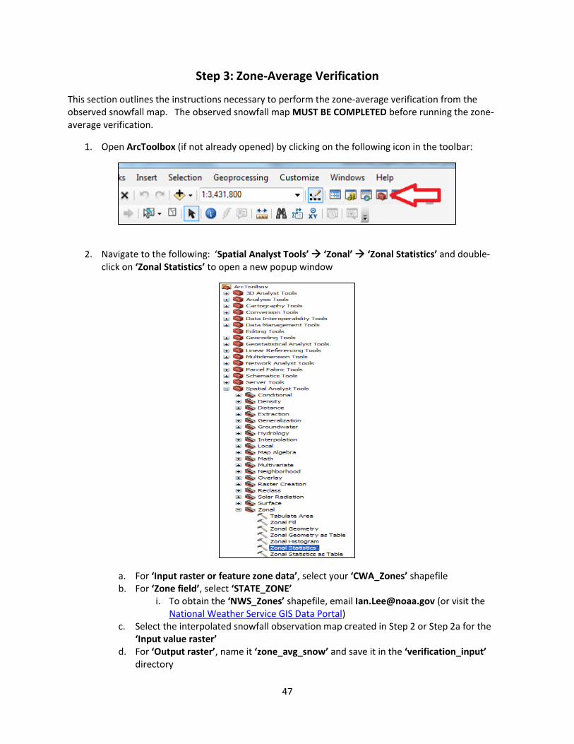
1. Open ArcToolbox (if not already opened) by clicking on the following icon in the toolbar:

2. Navigate to the following: ‘Spatial Analyst Tools’ ‘Zonal’ ‘Zonal Statistics’ and double-

click on ‘Zonal Statistics’ to open a new popup window

a. For ‘Input raster or feature zone data’, select your ‘CWA_Zones’ shapefile b. For ‘Zone field’, select ‘STATE_ZONE’

i. To obtain the ‘NWS_Zones’ shapefile, email Ian.Lee@noaa.gov (or visit the National Weather Service GIS Data Portal)

c. Select the interpolated snowfall observation map created in Step 2 or Step 2a for the ‘Input value raster’

d. For ‘Output raster’, name it ‘zone_avg_snow’ and save it in the ‘verification_input’ directory

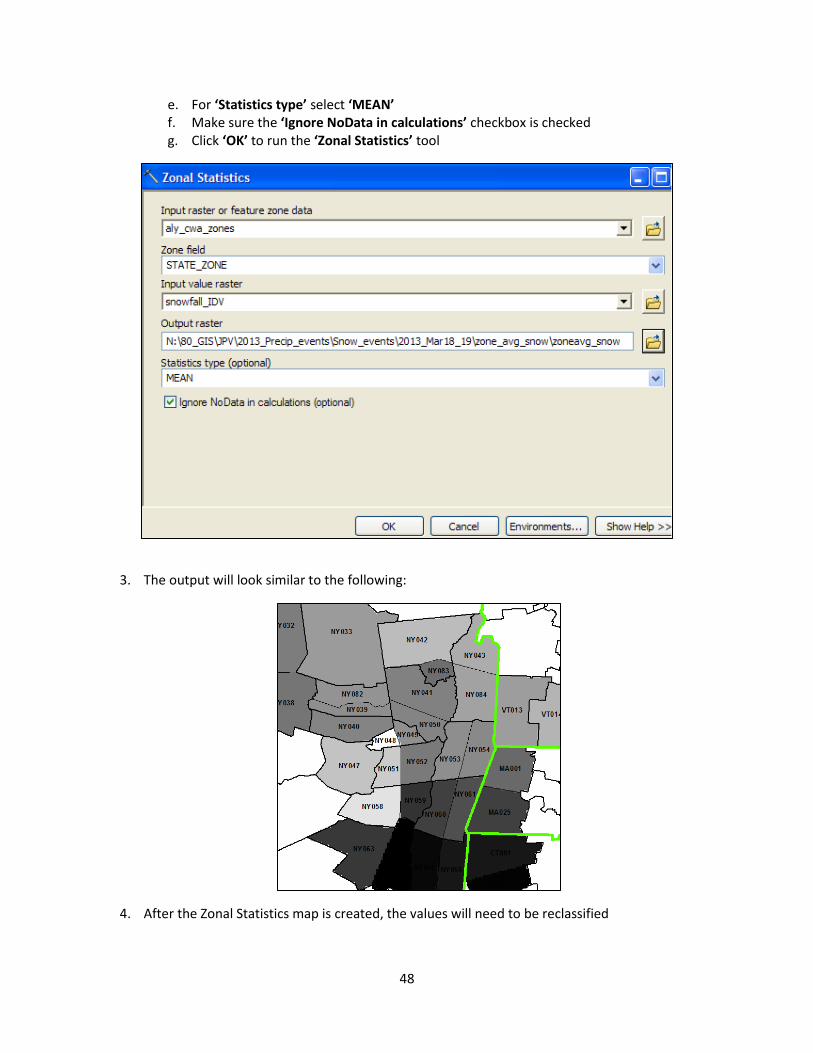
48

e. For ‘Statistics type’ select ‘MEAN’ f. Make sure the ‘Ignore NoData in calculations’ checkbox is checked g. Click ‘OK’ to run the ‘Zonal Statistics’ tool

2. 3. The output will look similar to the following:

4. After the Zonal Statistics map is created, the values will need to be reclassified

49

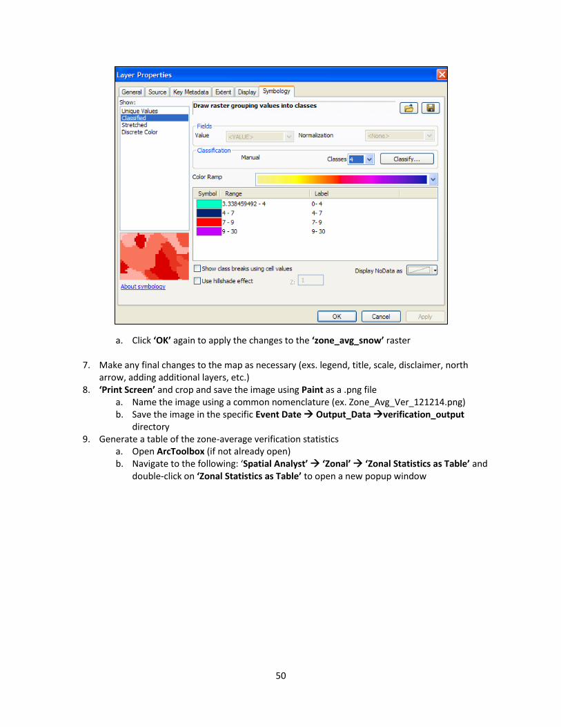
a. Right-click on the ‘zone_avg_snow’ raster layer and click on ‘Properties’ to open the ‘Layer Properties’ popup window

b. Click on the ‘Symbology’ tab (if not already selected) c. Make sure it is set to ‘Classified’ (left side of the popup window)

5. Choose ‘Manual Classification’ by selecting it from the ‘Classify’ button

6. Select ‘4 classes’ corresponding to the categories for snowfall verification: sub-advisory, advisory, 12-hour warning, 24-hour warning (these criteria will vary from office to office)

50

a. Click ‘OK’ again to apply the changes to the ‘zone_avg_snow’ raster

7. Make any final changes to the map as necessary (exs. legend, title, scale, disclaimer, north arrow, adding additional layers, etc.)

8. ‘Print Screen’ and crop and save the image using Paint as a .png file a. Name the image using a common nomenclature (ex. Zone_Avg_Ver_121214.png) b. Save the image in the specific Event Date Output_Data verification_output

directory 9. Generate a table of the zone-average verification statistics

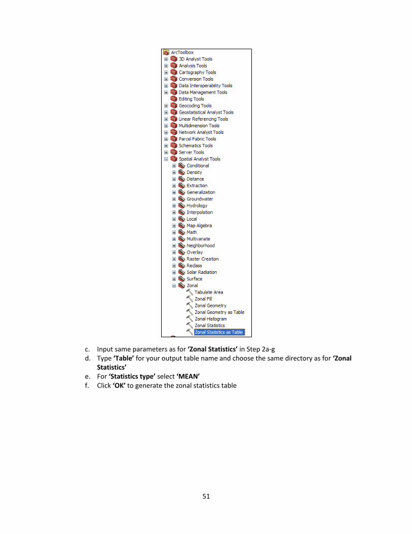
a. Open ArcToolbox (if not already open) b. Navigate to the following: ‘Spatial Analyst’ ‘Zonal’ ‘Zonal Statistics as Table’ and

double-click on ‘Zonal Statistics as Table’ to open a new popup window

51

c. Input same parameters as for ‘Zonal Statistics’ in Step 2a-g d. Type ‘Table’ for your output table name and choose the same directory as for ‘Zonal

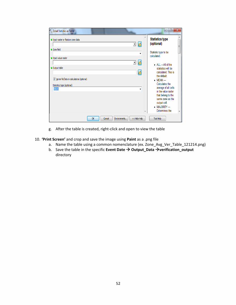
Statistics’ e. For ‘Statistics type’ select ‘MEAN’ f. Click ‘OK’ to generate the zonal statistics table

52

g. After the table is created, right-click and open to view the table

10. ‘Print Screen’ and crop and save the image using Paint as a .png file a. Name the table using a common nomenclature (ex. Zone_Avg_Ver_Table_121214.png) b. Save the table in the specific Event Date Output_Data verification_output

directory

53

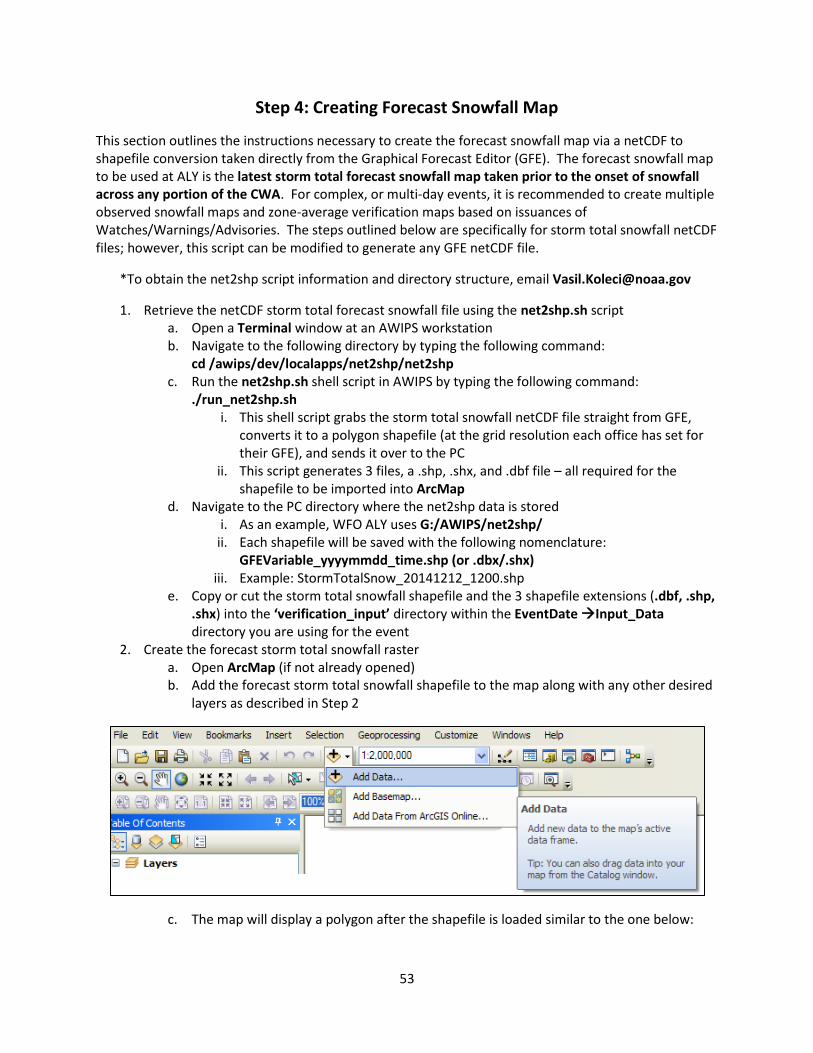
Step 4: Creating Forecast Snowfall Map

This section outlines the instructions necessary to create the forecast snowfall map via a netCDF to shapefile conversion taken directly from the Graphical Forecast Editor (GFE). The forecast snowfall map to be used at ALY is the latest storm total forecast snowfall map taken prior to the onset of snowfall across any portion of the CWA. For complex, or multi-day events, it is recommended to create multiple observed snowfall maps and zone-average verification maps based on issuances of Watches/Warnings/Advisories. The steps outlined below are specifically for storm total snowfall netCDF files; however, this script can be modified to generate any GFE netCDF file.

*To obtain the net2shp script information and directory structure, email Vasil.Koleci@noaa.gov

1. Retrieve the netCDF storm total forecast snowfall file using the net2shp.sh script a. Open a Terminal window at an AWIPS workstation b. Navigate to the following directory by typing the following command:

cd /awips/dev/localapps/net2shp/net2shp c. Run the net2shp.sh shell script in AWIPS by typing the following command:

./run_net2shp.sh i. This shell script grabs the storm total snowfall netCDF file straight from GFE,

converts it to a polygon shapefile (at the grid resolution each office has set for their GFE), and sends it over to the PC

ii. This script generates 3 files, a .shp, .shx, and .dbf file – all required for the shapefile to be imported into ArcMap

d. Navigate to the PC directory where the net2shp data is stored i. As an example, WFO ALY uses G:/AWIPS/net2shp/

ii. Each shapefile will be saved with the following nomenclature: GFEVariable_yyyymmdd_time.shp (or .dbx/.shx)

iii. Example: StormTotalSnow_20141212_1200.shp e. Copy or cut the storm total snowfall shapefile and the 3 shapefile extensions (.dbf, .shp,

.shx) into the ‘verification_input’ directory within the EventDate Input_Data directory you are using for the event

2. Create the forecast storm total snowfall raster a. Open ArcMap (if not already opened) b. Add the forecast storm total snowfall shapefile to the map along with any other desired

layers as described in Step 2

c. The map will display a polygon after the shapefile is loaded similar to the one below:

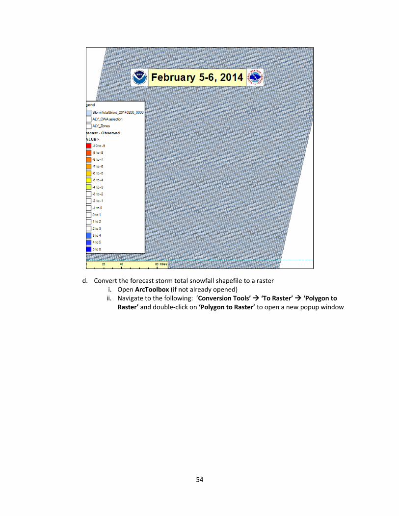
54

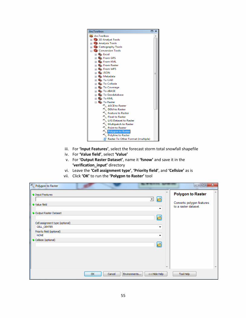
d. Convert the forecast storm total snowfall shapefile to a raster i. Open ArcToolbox (if not already opened)

ii. Navigate to the following: ‘Conversion Tools’ ‘To Raster’ ‘Polygon to Raster’ and double-click on ‘Polygon to Raster’ to open a new popup window

55

iii. For ‘Input Features’, select the forecast storm total snowfall shapefile iv. For ‘Value field’, select ‘Value’ v. For ‘Output Raster Dataset’, name it ‘fsnow’ and save it in the

‘verification_input’ directory vi. Leave the ‘Cell assignment type’, ‘Priority field’, and ‘Cellsize’ as is

vii. Click ‘OK’ to run the ‘Polygon to Raster’ tool

56

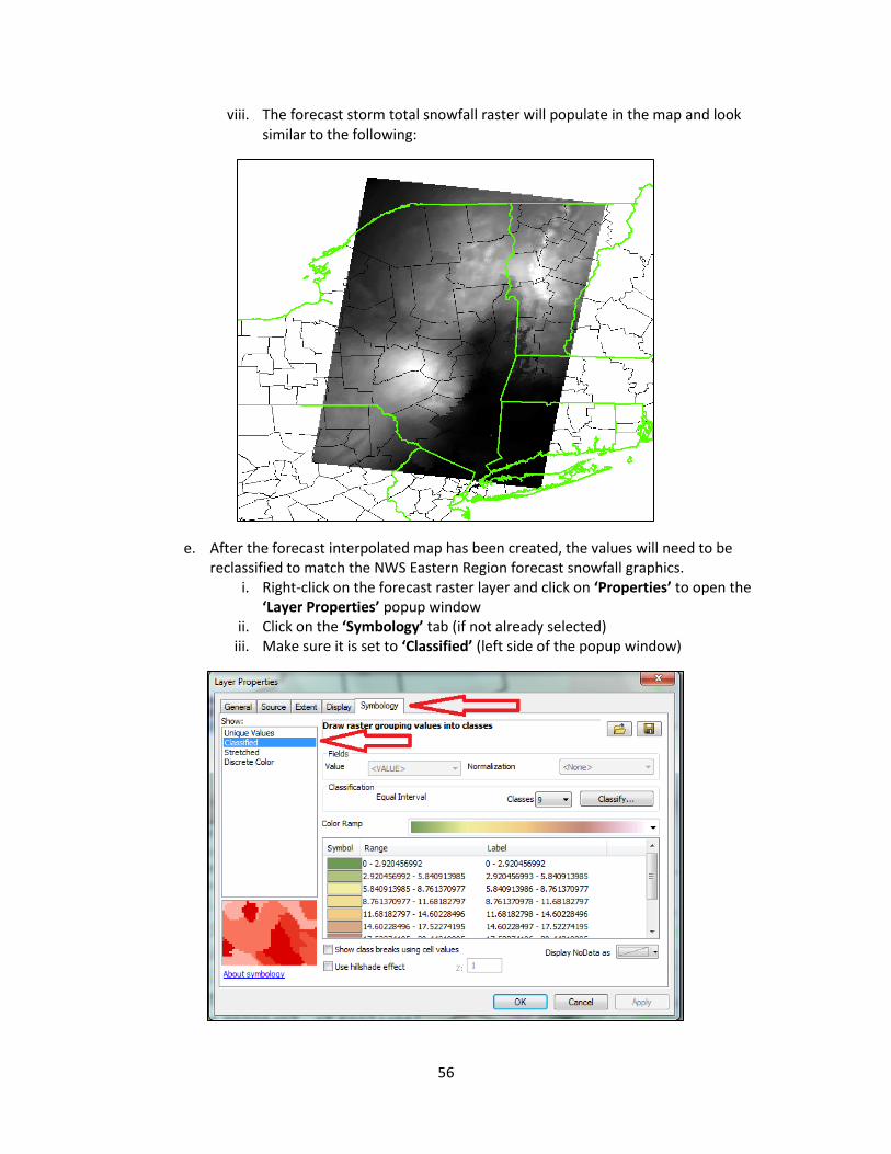
viii. The forecast storm total snowfall raster will populate in the map and look similar to the following:

e. After the forecast interpolated map has been created, the values will need to be reclassified to match the NWS Eastern Region forecast snowfall graphics.

i. Right-click on the forecast raster layer and click on ‘Properties’ to open the ‘Layer Properties’ popup window

ii. Click on the ‘Symbology’ tab (if not already selected) iii. Make sure it is set to ‘Classified’ (left side of the popup window)

57

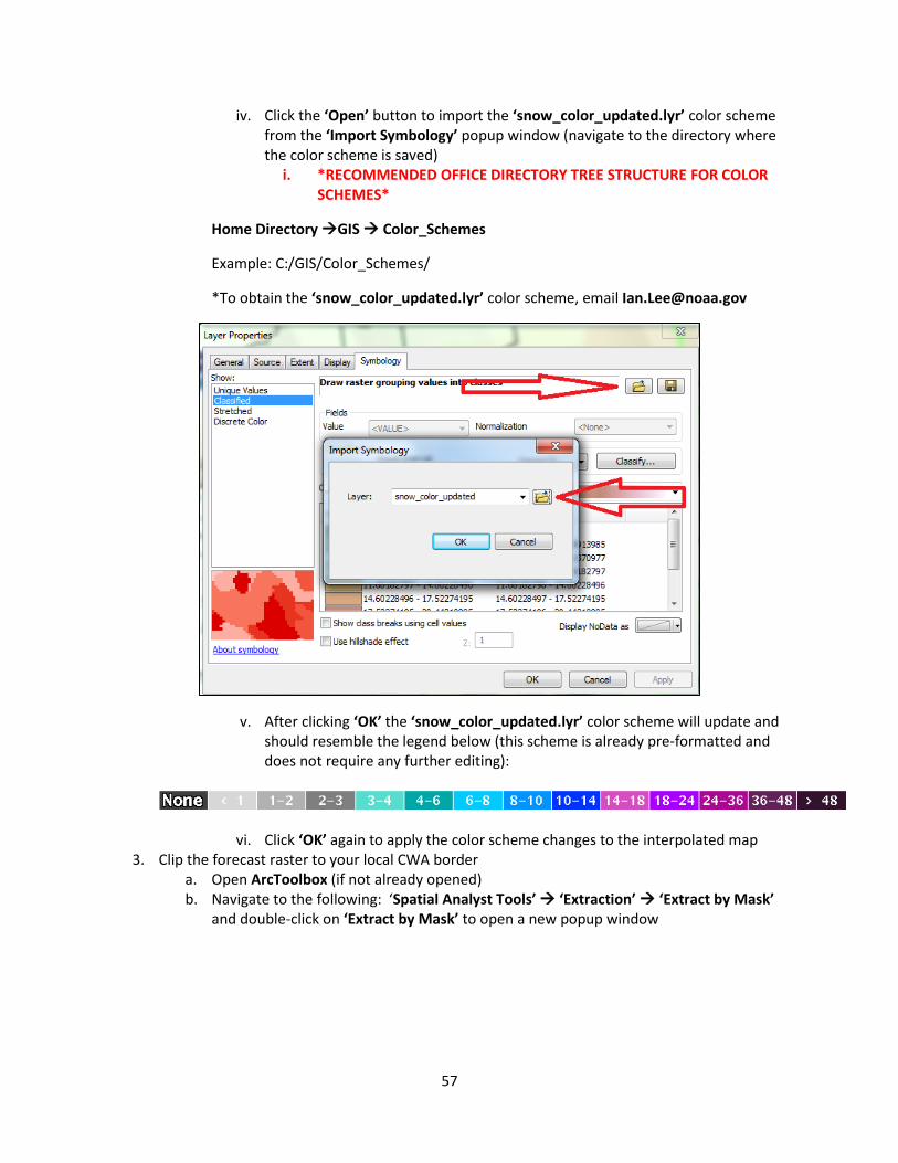
iv. Click the ‘Open’ button to import the ‘snow_color_updated.lyr’ color scheme from the ‘Import Symbology’ popup window (navigate to the directory where the color scheme is saved)

i. *RECOMMENDED OFFICE DIRECTORY TREE STRUCTURE FOR COLOR SCHEMES*

Home Directory GIS Color_Schemes

Example: C:/GIS/Color_Schemes/

*To obtain the ‘snow_color_updated.lyr’ color scheme, email Ian.Lee@noaa.gov

v. After clicking ‘OK’ the ‘snow_color_updated.lyr’ color scheme will update and should resemble the legend below (this scheme is already pre-formatted and does not require any further editing):

vi. Click ‘OK’ again to apply the color scheme changes to the interpolated map 3. Clip the forecast raster to your local CWA border

a. Open ArcToolbox (if not already opened) b. Navigate to the following: ‘Spatial Analyst Tools’ ‘Extraction’ ‘Extract by Mask’

and double-click on ‘Extract by Mask’ to open a new popup window

58

c. For ‘Input raster’, select the forecast raster d. For ‘Input raster or feature mask data’, select your office CWA border shapefile e. For ‘Output Raster’, name it ‘fsnow_extract’ and save it in the ‘verification_input’

directory f. Click ‘OK’ to run the ‘Extract by Mask’ tool

g. The output will display on the map confined to your office CWA border i. Turn off the fsnow raster layer, as you only want to see the clipped raster

h. After the forecast interpolated map has been clipped to the CWA border, the values will need to be reclassified to match the NWS Eastern Region forecast snowfall graphics.

i. Right-click on the forecast raster layer and click on ‘Properties’ to open the ‘Layer Properties’ popup window

ii. Click on the ‘Symbology’ tab (if not already selected) iii. Make sure it is set to ‘Classified’ (left side of the popup window)

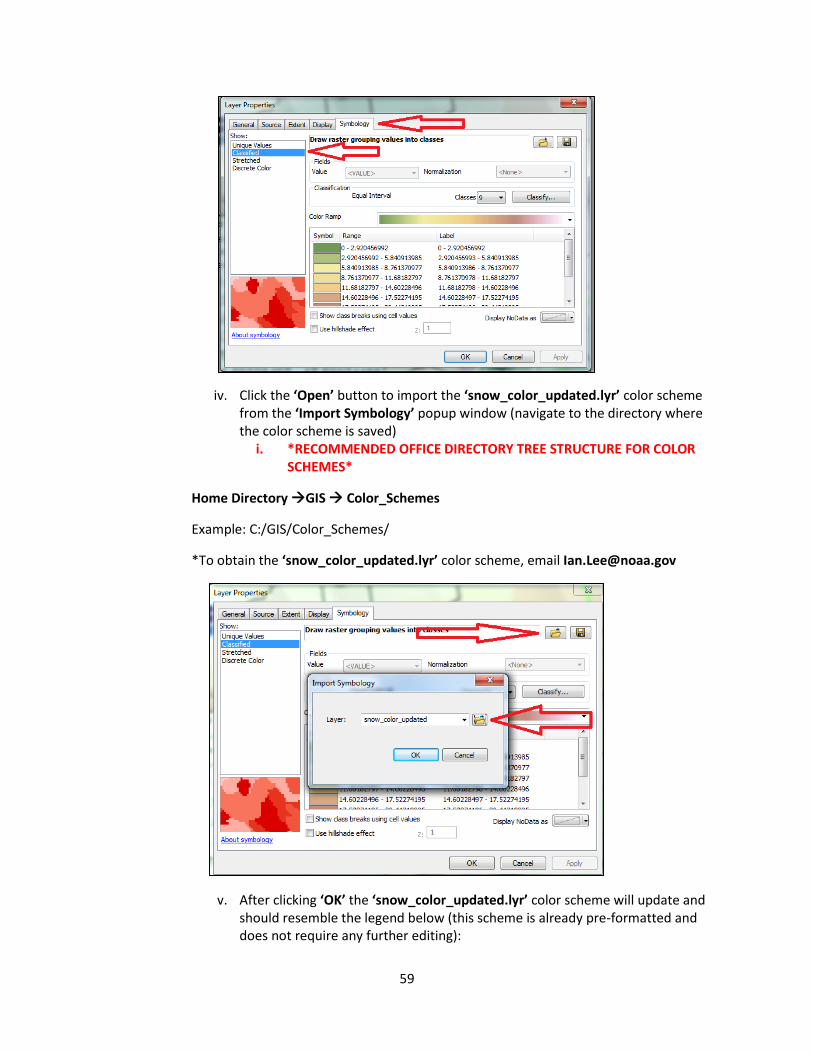
59

iv. Click the ‘Open’ button to import the ‘snow_color_updated.lyr’ color scheme from the ‘Import Symbology’ popup window (navigate to the directory where the color scheme is saved)

i. *RECOMMENDED OFFICE DIRECTORY TREE STRUCTURE FOR COLOR SCHEMES*

Home Directory GIS Color_Schemes

Example: C:/GIS/Color_Schemes/

*To obtain the ‘snow_color_updated.lyr’ color scheme, email Ian.Lee@noaa.gov

v. After clicking ‘OK’ the ‘snow_color_updated.lyr’ color scheme will update and should resemble the legend below (this scheme is already pre-formatted and does not require any further editing):

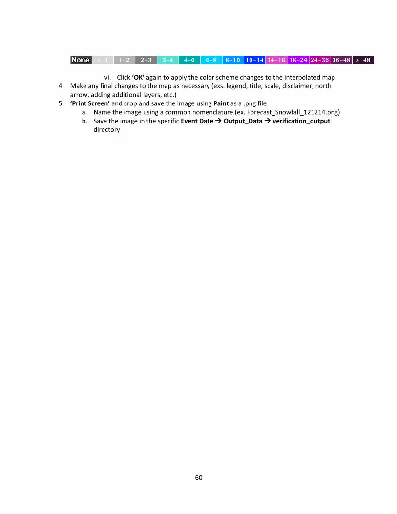
60

vi. Click ‘OK’ again to apply the color scheme changes to the interpolated map 4. Make any final changes to the map as necessary (exs. legend, title, scale, disclaimer, north

arrow, adding additional layers, etc.) 5. ‘Print Screen’ and crop and save the image using Paint as a .png file

a. Name the image using a common nomenclature (ex. Forecast_Snowfall_121214.png) b. Save the image in the specific Event Date Output_Data verification_output

directory

61

Step 5: Creating Forecast Error Map

This section outlines the instructions necessary to create the forecast error plot in order to see areas of overestimation and underestimation in the forecast. This error plot is recommended to be confined to your office local CWA boundary, in order to assess forecast error relative to your office CWA.

1. Clip the observed snowfall raster to your local CWA border a. Open ArcToolbox (if not already opened) b. Navigate to the following: ‘Spatial Analyst Tools’ ‘Extraction’ ‘Extract by Mask’

and double-click on ‘Extract by Mask’ to open a new popup window

c. For ‘Input raster’, select the observed snowfall raster created during Step 2/2a d. For ‘Input raster or feature mask data’, select your office CWA border shapefile e. For ‘Output Raster’, name it ‘obs_extract’ and save it in the ‘verification_input’

directory f. Click ‘OK’ to run the ‘Extract by Mask’ tool

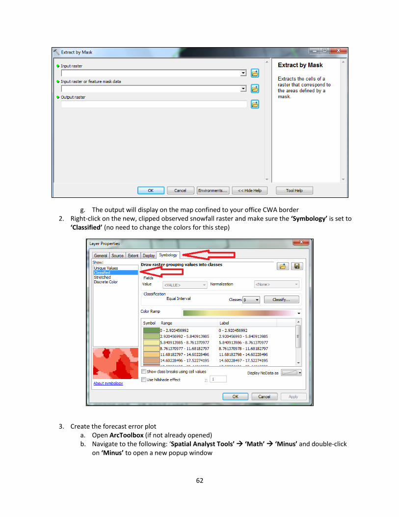
62

g. The output will display on the map confined to your office CWA border 2. Right-click on the new, clipped observed snowfall raster and make sure the ‘Symbology’ is set to

‘Classified’ (no need to change the colors for this step)

3. Create the forecast error plot

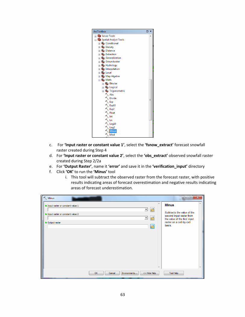
a. Open ArcToolbox (if not already opened) b. Navigate to the following: ‘Spatial Analyst Tools’ ‘Math’ ‘Minus’ and double-click

on ‘Minus’ to open a new popup window

63

c. For ‘Input raster or constant value 1’, select the ‘fsnow_extract’ forecast snowfall raster created during Step 4

d. For ‘Input raster or constant value 2’, select the ‘obs_extract’ observed snowfall raster created during Step 2/2a

e. For ‘Output Raster’, name it ‘error’ and save it in the ‘verification_input’ directory f. Click ‘OK’ to run the ‘Minus’ tool

i. This tool will subtract the observed raster from the forecast raster, with positive results indicating areas of forecast overestimation and negative results indicating areas of forecast underestimation.

64

4. Customize the color scale and ranges by reclassifying a. Right-click on the ‘error’ raster and click on ‘Properties’

b. Click on the ‘Symbology’ tab and make sure it is set to ‘Classified’

c. Leave the number of ‘Classes’ alone – it will automatically default to the appropriate number based on the range of values in the ‘error’ raster

d. Change the color ramp to the color ramp shown in the above image e. Left-click where it says ‘Symbol’ and click ‘Flip Colors’ so that cooler colors represent

negative values, or underestimation of the forecast and warmer colors represent positive values, or overestimation of the forecast

65

f. Click ‘OK’ to apply the changes

5. Make any final changes to the map as necessary (exs. Legend, title, scale, disclaimer, north arrow, adding additional layers, etc.)

6. ‘Print Screen’ and crop and save the image using Paint as a .png file a. Name the image using a common nomenclature (ex. Forecast_Snowfall_121214.png) b. Save the image in the specific Event Date Output_Data verification_output

directory