International Journal of Computer Vision manuscript No.(will be inserted by the editor)

A Gromov-Hausdorff framework with diffusion geometryfor topologically-robust non-rigid shape matching

Alexander M. Bronstein,† Michael M.

Bronstein,† Mona Mahmoudi,‡ Ron Kimmel,†

and Guillermo Sapiro‡

the date of receipt and acceptance should be inserted later

Abstract In this paper, the problem of non-rigid shape recognition is viewed from the

perspective of metric geometry, and the applicability of diffusion distances within the

Gromov-Hausdorff framework is explored. While the commonly used geodesic distance

exploits the shortest path between points on the surface, the diffusion distance averages

all paths connecting between the points. The diffusion distance provides an intrinsic

distance measure which is robust, in particular to topological changes. Such changes

may be a result of natural non-rigid deformations, as well as acquisition noise, in the

form of holes or missing data, and representation noise due to inaccurate mesh con-

struction. The presentation of the proposed framework is complemented with numerous

examples demonstrating that in addition to the relatively low complexity involved in

the computation of the diffusion distances between surface points, its recognition and

matching performances favorably compare to the classical geodesic distances in the

presence of topological changes between the non-rigid shapes.

Keywords Non-rigid shape matching, Diffusion geometry, Gromov-Hausdorff

distance.

1 Introduction

Non-rigid shapes are ubiquitous in the world we live in, from microscopic bacteria to

tissues and parts of our body. Since pattern recognition applications need to deal with

objects encountered in everyday life, non-rigid shape analysis has become important in

many modern applications, such as object retrieval and recognition, surface matching,

navigation, and target detection and recognition. One of the cornerstone problems in

This work is partially supported by NSF, ONR, NGA, ARO, DARPA, NIH, and by the IsraelScience Foundation (ISF grant No. 623/08).

† Novafora, Inc., and Department of Computer Science, Technion – Israel Institute ofTechnology. E-mail: bron@cs.technion.ac.il, mbron@cs.technion.ac.il, ron@cs.technion.ac.il

‡ Department of Electrical and Computer Engineering, University of MinnesotaE-mail: mahmo022@umn.edu, guille@umn.edu

2

the analysis of non-rigid shapes is the problem of shape similarity : given two objects,

we need to tell how similar or dissimilar they are. This can be quantitatively expressed

as a distance between two shapes. The main difficulty in such a comparison stems from

the immense number of degrees of freedom present in the problem as a result of possible

deformations that the non-rigid shapes can undergo.

A common way the problem of non-rigid shape similarity has been approached in

the pattern recognition literature is to try to find a representation of shapes which is

invariant to a given class of deformations [37]. Using such a representation, it is then

possible to compare shapes regardless of their deformations, when these deformations

are limited to the given class. Riemannian geometry is of help in finding such invariant

representations [15]. It is well-known, for example, that the intrinsic properties of a

shape remain invariant under inelastic deformations, i.e., deformations that do not

“stretch” or “tear” the object. Many recent papers, e.g., [16,17,20,26,29,35,36,38–40,

42,45], exploit this fact in order to construct deformation-invariant shape distances

and surface matching techniques.

Elad and Kimmel [16] introduced a method for the recognition of 3D shapes based

on Euclidean embedding, extending previous efforts by Schwartz et al. [42] (see also

[45]). The key idea of the method is to consider a shape as a metric space, whose metric

structure is defined by the (natural) geodesic distances between pairs of points on the

shape. 1 Geodesic distances, being an intrinsic property of the shape, are invariant

to any inelastic deformation the shape can undergo (or, using metric geometry ter-

minology, we can say that such deformations are isometric or metric-preserving when

considering geodesic distances). Two non-rigid shapes are compared by first having

their respective geodesic metric structures mapped into a low-dimensional Euclidean

space using multidimensional scaling (MDS) [14], and then rigidly matching the result-

ing images (called canonical forms). MDS allows to “undo” the non-rigid deformations

of the shapes, leading to a bending-invariant shape comparison framework based on

the pairwise geodesic distances. This method has been used in three-dimensional face

recognition [4], analysis of articulated two-dimensional shapes and images [27,28], tex-

ture mapping and object morphing [7,19,49], and shape segmentation [23].

Due to the fact that the canonical forms method uses an intermediate metric space

to compare two shapes, an inaccuracy is introduced, as it is theoretically impossible

to embed a generic metric structure into a finite-dimensional Euclidean space without

distorting it. It was shown empirically in [8,46] that using spaces with non-Euclidean

(non-flat) geometry makes it possible to obtain more accurate representations, but can

not avoid the error completely.

In [35], Memoli and Sapiro proposed a metric framework for non-rigid shape com-

parison based on the Gromov-Hausdorff distance. This distance was introduced by

Mikhail Gromov, [18], as a way to compute similarity between metric spaces. Using

the Gromov-Hausdorff formalism, the comparison of two shapes can be posed as direct

comparison of pairwise distances on the shapes (basically, in the discrete case, the com-

parison up to permutations of the corresponding pairwise distance matrices or their

corresponding submatrices). Since no fixed intermediate space is used, the representa-

tion error inherent to canonical forms can be avoided. The Gromov-Hausdorff distance

computation is an NP-hard problem, and together with a number of theoretical results,

Memoli and Sapiro proposed a practical approximation scheme (with explicit proba-

1 Recall that the geodesic distance between two points is the length of the shortest path,traveling on the surface of the shape, that connects the points.

3

bilistic bounds connecting the approximation to the actual Gromov-Hausdorff distance

and the number of available sample points).

According to an alternative but mathematically equivalent definition [11,35], the

Gromov-Hausdorff distance computation can be posed as measuring the distortion of

embedding one metric space into another. Bronstein et al. [5,6], observing the connec-

tion between this formulation of the Gromov-Hausdorff distance and MDS, proposed an

efficient computation of such embedding based on a continuous optimization problem

(energy minimization), referred to as generalized MDS (GMDS). This method follows

the line of thought of embedding into non-Euclidean spaces,2 and can be considered a

natural extension thereof. This is the computational technique that will be exploited

for the examples in this paper.

All the aforementioned contributions considered only geodesic distances as the in-

variant used to intrinsically compare non-rigid shapes. This is motivated by a number

of fundamental reasons. First, many natural object deformations can be approximated

as inelastic ones. Thus, methods based on geodesic distances allow good shape recog-

nition accuracy. Second, there exists a plethora of efficient numerical methods for the

computation of geodesic distances for diverse shape representations [3,24,33,34,44,48].

The notable drawback of the geodesic distances is their sensitivity to topological

transformations. By modifying the connectivity of the shape, one can significantly alter

the paths between points, and in particular the shortest one, which in turn, can result

in significant changes of the geodesic distances. Inconsistent topology or “topological

noise” are common phenomena in shapes acquired using 3D scanners or obtained as

a result of point cloud triangulation [47]. Thus, in order to be able to deal with real-

life data, it is important for shape similarity methods to be topology-invariant (or at

least topologically robust). Of course, topological changes can result from natural non-

rigid deformations as well, e.g., bending of an open hand until the finger tips touch. A

practically useful shape recognition system should be able to somehow deal with these

transformations.

It should be noted, however, that the metric model of shapes allows to represent a

shape as a generic metric space with any metric. Also, neither the canonical forms nor

the Gromov-Hausdorff distance are necessarily limited to geodesic distances. Using an-

other intrinsic distance, insensitive or robust to topological changes, instead of geodesic

ones, could potentially make these methods cope with topological noise and topolog-

ical deformations in general. In [9,10], Bronstein et al. showed that using Euclidean

distances (which are robust to topology changes but not invariant or even robust to

non-rigid deformations), and geodesic distances (which are invariant to non-rigid de-

formations but not to topology changes) together in a framework resemblant both of

the GMDS and iterative closest point (ICP) algorithms [2,12], allows to obtain a shape

similarity method more robust to topological changes than the one obtained with the

geodesic distances alone.3

Motivated by the generality of the metric framework, and the need to add topologi-

cal insensitivity to non-rigid shape recognition, in this paper we propose to use diffusion

geometry in the Gromov-Hausdorff framework. Diffusion distances, introduced by La-

2 Instead of embedding each shape into Euclidean, hyperbolic, or spherical spaces, as clas-sically done in MDS, the embedding is done from one shape into the other.

3 Also, it was shown in [9,10] that the Gromov-Hausdorff type distance between shapesmodeled as metric spaces with Euclidean geometry allows to obtain an alternative formulation,and then use GMDS as a computation method for the ICP method, a classical approach forrigid shape comparison (for more detailed analysis, see [32]).

4

fon et al. [13,25], are related to the probability of traveling on the surface from one

point to another in a fixed number of random steps (random walk). There are a number

of reasons that lead us to prefer these distances over minimal geodesics when we deal

with topological noise and changes. First, the diffusion distance is an average length of

paths connecting two points on the shape, while the geodesic distance is the length of

the shortest path. This naturally makes diffusion distances less sensitive to topological

changes [29,41]. Secondly, both diffusion and geodesic distance are intrinsic, thus in-

variant to inelastic deformations. Finally, diffusion distance can be efficiently computed

from the eigenvalues of a discrete approximation to the Laplace-Beltrami operator (or

simply the eigenvalues of a weighted connectivity matrix). The reader is referred to

[22,30,41] for some recent works on 3D shape recognition based on spectral methods,

both for geodesic matrices and the Laplace-Beltrami operator, which is closely related

to the diffusion distance [21]. The diffusion distance was also exploited for 3D point

cloud recognition using the framework of distance distributions in [29]. Combining the

Gromov-Hausdorff framework with diffusion distances leads to a non-rigid shape com-

parison and matching approach which is robust to topological alterations such as holes

and point-wise connectivity changes, as demonstrated in this paper.

The remainder of this paper is organized as follows. In Section 2 we present the

metric approach to shape recognition and the Gromov-Hausdorff framework. Section 3

describes the basic diffusion distance theory. Section 4 is devoted to the numerical com-

putation of the proposed shape distance based on the GMDS algorithm, and Section 5

presents experimental results. Finally, Section 6 concludes the paper.

2 Metric approach for shape recognition

In this section we present some basic concepts that constitute the core of the metric

approach for shape recognition, staying mostly at the intuitive level. For a rigorous

and insightful treatment of the topic, the reader is referred to [11].

2.1 Basic notions in metric geometry

We model a non-rigid shape as a metric space (X, dX), where X is a two-dimensional

smooth compact connected and complete Riemannian surface (possibly with boundary)

embedded into R3, and dX : X×X → R is a metric measuring distances between pairs

of points on X. The key idea of the metric approach is to compare shapes as metric

spaces. Two shapes (X, dX) and (Y, dY ) are similar if the metrics between pairs of

corresponding points on X and Y coincide, i.e., there exists a bijective map ϕ : X → Y

such that dY ◦ (ϕ×ϕ) = dX . Such a ϕ is called an isometry and X and Y in this case

are said to be isometric. Isometry implies that in terms of intrinsic metric geometry,

the two shapes are indistinguishable and thus are equivalent.

The notion of isometry can be relaxed in order to define similarity of shapes. We

will refer to a set C ⊂ X×Y of pairs such that for every x ∈ X there exists at least one

y ∈ Y such that (x, y) ∈ C, and similarly for every y ∈ Y there exists an x ∈ X such

that (x, y) ∈ C, as a correspondence between X and Y . Note that a correspondence C

is not necessarily a function. We can define the distortion of the correspondence as the

discrepancy between the corresponding metrics,

dis(C) := sup(x,y),(x′,y′)∈C

∣∣dX(x, x′)− dY (y, y′)∣∣ .

5

We say that the shapes X and Y are ε-isometric if there exists a correspondence C

with dis(C) ≤ ε. Such a C is called an ε-isometry. ε-isometry can be regarded as a

criterion of shape similarity. For small values of ε, the shapes are similar, and for large

values of ε, the shapes are dissimilar.

2.2 Gromov-Hausdorff distance

A very elegant framework to represent similarity of metric spaces as a distance was

proposed by Gromov [11,18] and introduced into the non-rigid shape recognition area in

[35]. For compact surfaces and our shape recognition framework, the Gromov-Hausdorff

distance can be expressed in terms of the distortion obtained by embedding one surface

into another,

dGH(X, Y ) :=1

2infC

dis (C),

where the infimum is taken over all correspondence C, and dis (C) is the distortion

defined above.

The Gromov-Hausdorff distance is a metric on the quotient space of metric spaces

under the isometry relation, and thus, in the context of the metric space model for shape

recognition, is a good candidate for a shape distance [35]. Being a metric particularly

implies that dGH(X, Y ) = 0 if and only if X and Y are isometric. More generally,

if dGH(X, Y ) ≤ ε, then X and Y are 2ε-isometric and conversely, if X and Y are

ε-isometric, then dGH(X, Y ) ≤ 2ε [11].

2.3 Choice of a metric

The metric approach we have described and the Gromov-Hausdorff distance do not

prescribe any particular choice of the metric dX . In general, dX is independent of X

and can be defined quite arbitrarily. There are, however, two natural choices of dX .

The first choice is the geodesic metric, measuring the length of the shortest intrinsic

path between a pair of points, constructing the intrinsic geometry of X. The second

choice is the extrinsic Euclidean metric, measuring the length of a line in R3 connecting

two points on X that relates to the extrinsic geometry in which X is embedded, i.e.,

R3 (see also [32]).

Extrinsic geometry is invariant to rigid transformations of the shape (rotation,

translation, and reflection), which preserve Euclidean distances. However, nonrigid de-

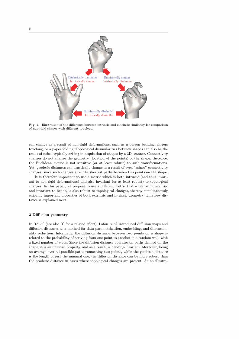
formations may change the extrinsic geometry (see example in Fig. 1). As a result, the

Euclidean metric is not suitable for the comparison of shapes with significant bending

or other type of non-rigid deformations. The intrinsic geometry on the other hand is

invariant to inelastic shape deformations which do not “stretch”or “tear” the shape.

As a particular case, it is also invariant to rigid transformations (see also [32]). There-

fore, the geodesic metric is a good choice for comparing non-rigid shapes, as has been

confirmed by numerous results as those mentioned in the introduction.

Another important type of transformations a shape can undergo are those changing

the shape topology. Omitting formal definitions, the topology of X can be thought of as

a collection of neighborhoods of every point on X. This defines the connectivity of the

shape - which points can be reached by a small step from a neighbor point. Topology

6

Intrinsically dissimilar

Extrinsically dissimilar

Intrinsically dissimilar

Extrinsically similar

Intrinsically similar

Extrinsically dissimilar

Fig. 1 Illustration of the difference between intrinsic and extrinsic similarity for comparisonof non-rigid shapes with different topology.

can change as a result of non-rigid deformations, such as a person bending, fingers

touching, or a paper folding. Topological dissimilarities between shapes can also be the

result of noise, typically arising in acquisition of shapes by a 3D scanner. Connectivity

changes do not change the geometry (location of the points) of the shape, therefore,

the Euclidean metric is not sensitive (or at least robust) to such transformations.

Yet, geodesic distances can drastically change as a result of even “minor” connectivity

changes, since such changes alter the shortest paths between two points on the shape.

It is therefore important to use a metric which is both intrinsic (and thus invari-

ant to non-rigid deformations) and also invariant (or at least robust) to topological

changes. In this paper, we propose to use a different metric that while being intrinsic

and invariant to bends, is also robust to topological changes, thereby simultaneously

enjoying important properties of both extrinsic and intrinsic geometry. This new dis-

tance is explained next.

3 Diffusion geometry

In [13,25] (see also [1] for a related effort), Lafon et al. introduced diffusion maps and

diffusion distances as a method for data parametrization, embedding, and dimension-

ality reduction. Informally, the diffusion distance between two points on a shape is

related to the probability of arriving from one point to another in a random walk with

a fixed number of steps. Since the diffusion distance operates on paths defined on the

shape, it is an intrinsic property, and as a result, is bending-invariant. Moreover, being

an average over all possible paths connecting two points, while the geodesic distance

is the length of just the minimal one, the diffusion distance can be more robust than

the geodesic distance in cases where topological changes are present. As an illustra-

7

tion, imagine the hand shape and two points on the tips of the index finger and the

thumb. If the two fingertips are not touching, then both geodesic and diffusion dis-

tances between the two points are large, as all paths connecting the two points travel

throughout the whole hand. Yet, if the hand is bent in such a way that the fingertips

touch each other, the minimal geodesic will “re-route” itself through the “shortcut”

across the fingertips instead of going though the hand, leading to a significant change

in the geodesic distance. For the diffusion distance, this new path added as a result of

the topology change is averaged with the other paths, which reduces the effect of such

a change. Obviously, the lesser sensitivity to topological changes attributed to the aver-

aging property of the diffusion distance, comes at the expense of a potential reduction

in discriminative power, as it usually happens in a trade off between invariance and

discriminativity. However, we have not observed any significant loss of discriminativity

in the experiments in this paper, nor in [29] (see the discussion in Section 6).

Besides the above properties, the diffusion distance is a metric, and thus, a valid

candidate for the definition of a metric space used in the Gromov-Hausdorff shape

model. This stems from the fact that following the diffusion geometry framework, the

3D shape can be embedded into a (theoretically infinite-dimensional) Euclidean space

by means of an eigenmap referred to as diffusion map in [13,25]. The Euclidean distance

in this space equals the diffusion distance measured on the original shape (see next).

Formally, in order to compute the diffusion distance, we first construct a non-

negative symmetric affinity function k(x, y) ≥ 0 over all pairs of points x, y on the

shape. In the discrete setting, the shape may be represented as a triangular mesh,

point cloud, or parametric surface. For the exposition simplicity, we regard the shape

X as a finite set of points. The affinity function in this case can be represented as an

N × N matrix K, where N is the number of samples.4 The matrix is symmetric and

has non-zero values.

Next, we define

p(x, y) :=k(x, y)

v(x), (1)

where v(x) :=∑

y k(x, y). Note that while still positive, p(x, y) is not symmetric any

longer, therefore, we define a symmetric version,

p(x, y) := p(x, y)

(v(x)

v(y)

)1/2

. (2)

It is easy to verify that ∑x

p(x, y) = 1. (3)

This allows to interpret the N × N matrix P = (p(x, y)) as a transition matrix of

a random walk (Markov process) on X, where p(x, y) is the probability of transition

from point x to y in one step. Using the random walk formulation, the probability of

transition from x to y in m steps is given by the m-th power of the matrix P . The

element p(m)(x, ·) of the matrix Pm can be thought of as a “bump” centered at x and

of width proportional to m.

Then, the diffusion distance, defined as

d2m(x, y) :=

∑

z∈X

|p(m)(x, z)− p(m)(y, z)|2, (4)

4 In the continuous case, matrices are replaced by operators and vectors by functions. Seemore rigorous definitions in [13,25].

8

can be thought of as a distance between two bumps. It is inversely related to the

connectivity of points x and y by paths of length m (i.e., if there are many such paths

connecting x and y, the distance d2m(x, y) is small).

Using eigendecomposition of P , we can expand p(x, y) as

p(x, y) =

N∑

i=0

λ2i φi(x)φi(y), (5)

where λ20 = 1 ≥ λ2

1 ≥ λ22 ≥ ... ≥ λ2

N are the eigenvalues (note that the eigenvalues are

squared for convenience), of the matrix P , and φl are the corresponding eigenvectors.

Therefore, for the elements of the matrix Pm we obtain

p(m)(x, y) =

N∑

i=0

λ2mi φi(x)φi(y). (6)

The eigenmap

Φm(x) :=

λm0 φ0(x)

λm1 φ1(x)

λm2 φ2(x)

...

, (7)

defined by the eigenvalues and eigenvectors of P , and mapping points from X to the

Euclidean space, was termed diffusion map in [13]. It is well known and easy to see

that the Euclidean distance in the diffusion map space equals to the diffusion distance,

i.e.,

‖Φm(x)− Φm(y)‖2 = d2m(x, y). (8)

As a result, the diffusion distance is a metric and therefore can be used to define a

valid metric space in our framework.

For completeness, we should mention that in order to account for non-uniform

sampling density of X, the affinity function k(x, y) is further normalized,

k(x, y) =k(x, y)

v(x)v(y), (9)

and the normalized affinity function k is used instead of k [25]. The choice of k(x, y)

itself is, to a large extent, arbitrary (in particular when considering experimental re-

sults, while more restricted selections are needed for some of the critical theoretical

results connecting this to the Laplace-Beltrami operator to hold). Typically, the Gaus-

sian kernel k(x, y) = exp(−‖x− y‖2/σ2) is used, where σ depends on the shape and its

sampling, e.g., it can be the average of Euclidean distances between all pairs of points

in the shape [29]. Other kernels can be used as well. For the experiments in this paper,

we found sufficient to use the kernel k(xi, xj) = 1 if xi and xj are connected and zero

otherwise (leading to a very sparse matrix K). The time constant m = 50 was used

and density was assumed to be constant.

9

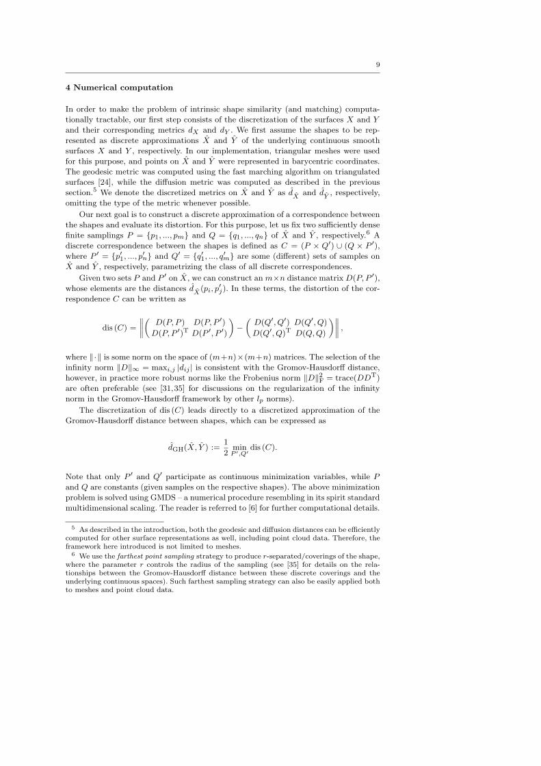
4 Numerical computation

In order to make the problem of intrinsic shape similarity (and matching) computa-

tionally tractable, our first step consists of the discretization of the surfaces X and Y

and their corresponding metrics dX and dY . We first assume the shapes to be rep-

resented as discrete approximations X and Y of the underlying continuous smooth

surfaces X and Y , respectively. In our implementation, triangular meshes were used

for this purpose, and points on X and Y were represented in barycentric coordinates.

The geodesic metric was computed using the fast marching algorithm on triangulated

surfaces [24], while the diffusion metric was computed as described in the previous

section.5 We denote the discretized metrics on X and Y as dX

and dY

, respectively,

omitting the type of the metric whenever possible.

Our next goal is to construct a discrete approximation of a correspondence between

the shapes and evaluate its distortion. For this purpose, let us fix two sufficiently dense

finite samplings P = {p1, ..., pm} and Q = {q1, ..., qn} of X and Y , respectively.6 A

discrete correspondence between the shapes is defined as C = (P × Q′) ∪ (Q × P ′),where P ′ = {p′1, ..., p′n} and Q′ = {q′1, ..., q′m} are some (different) sets of samples on

X and Y , respectively, parametrizing the class of all discrete correspondences.

Given two sets P and P ′ on X, we can construct an m×n distance matrix D(P, P ′),whose elements are the distances d

X(pi, p

′j). In these terms, the distortion of the cor-

respondence C can be written as

dis (C) =

∥∥∥∥(

D(P, P ) D(P, P ′)D(P, P ′)T D(P ′, P ′)

)−

(D(Q′, Q′) D(Q′, Q)

D(Q′, Q)T D(Q, Q)

)∥∥∥∥ ,

where ‖·‖ is some norm on the space of (m+n)×(m+n) matrices. The selection of the

infinity norm ‖D‖∞ = maxi,j |dij | is consistent with the Gromov-Hausdorff distance,

however, in practice more robust norms like the Frobenius norm ‖D‖2F = trace(DDT)

are often preferable (see [31,35] for discussions on the regularization of the infinity

norm in the Gromov-Hausdorff framework by other lp norms).

The discretization of dis (C) leads directly to a discretized approximation of the

Gromov-Hausdorff distance between shapes, which can be expressed as

dGH(X, Y ) :=1

2min

P ′,Q′dis (C).

Note that only P ′ and Q′ participate as continuous minimization variables, while P

and Q are constants (given samples on the respective shapes). The above minimization

problem is solved using GMDS – a numerical procedure resembling in its spirit standard

multidimensional scaling. The reader is referred to [6] for further computational details.

5 As described in the introduction, both the geodesic and diffusion distances can be efficientlycomputed for other surface representations as well, including point cloud data. Therefore, theframework here introduced is not limited to meshes.

6 We use the farthest point sampling strategy to produce r-separated/coverings of the shape,where the parameter r controls the radius of the sampling (see [35] for details on the rela-tionships between the Gromov-Hausdorff distance between these discrete coverings and theunderlying continuous spaces). Such farthest sampling strategy can also be easily applied bothto meshes and point cloud data.

10

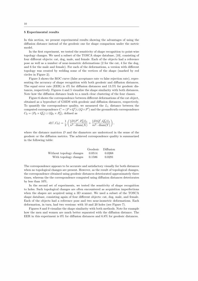
5 Experimental results

In this section, we present experimental results showing the advantages of using the

diffusion distance instead of the geodesic one for shape comparison under the metric

model.

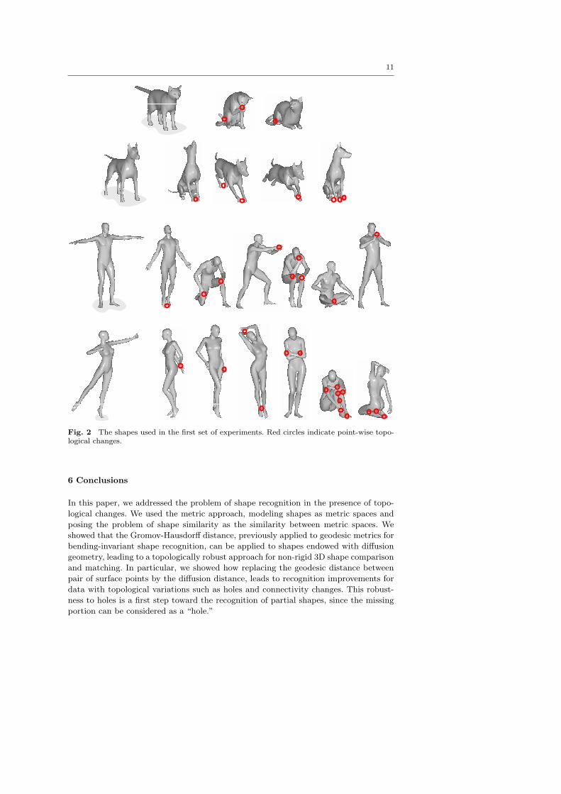
In the first experiment, we tested the sensitivity of shape recognition to point-wise

topology changes. We used a subset of the TOSCA shape database, [10], consisting of

four different objects: cat, dog, male, and female. Each of the objects had a reference

pose as well as a number of near-isometric deformations (2 for the cat, 4 for the dog,

and 6 for the male and female). For each of the deformations, a version with different

topology was created by welding some of the vertices of the shape (marked by red

circles in Figure 2).

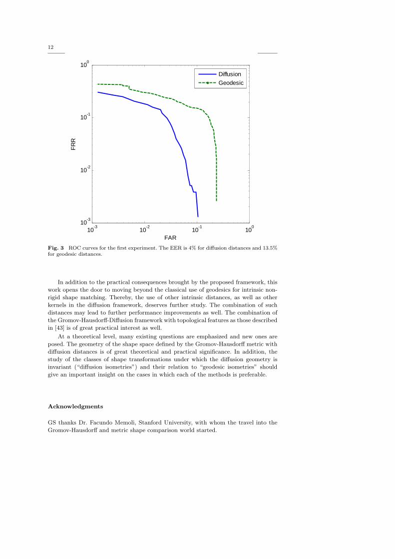
Figure 3 shows the ROC curve (false acceptance rate vs false rejection rate), repre-

senting the accuracy of shape recognition with both geodesic and diffusion distances.

The equal error rate (EER) is 4% for diffusion distances and 13.5% for geodesic dis-

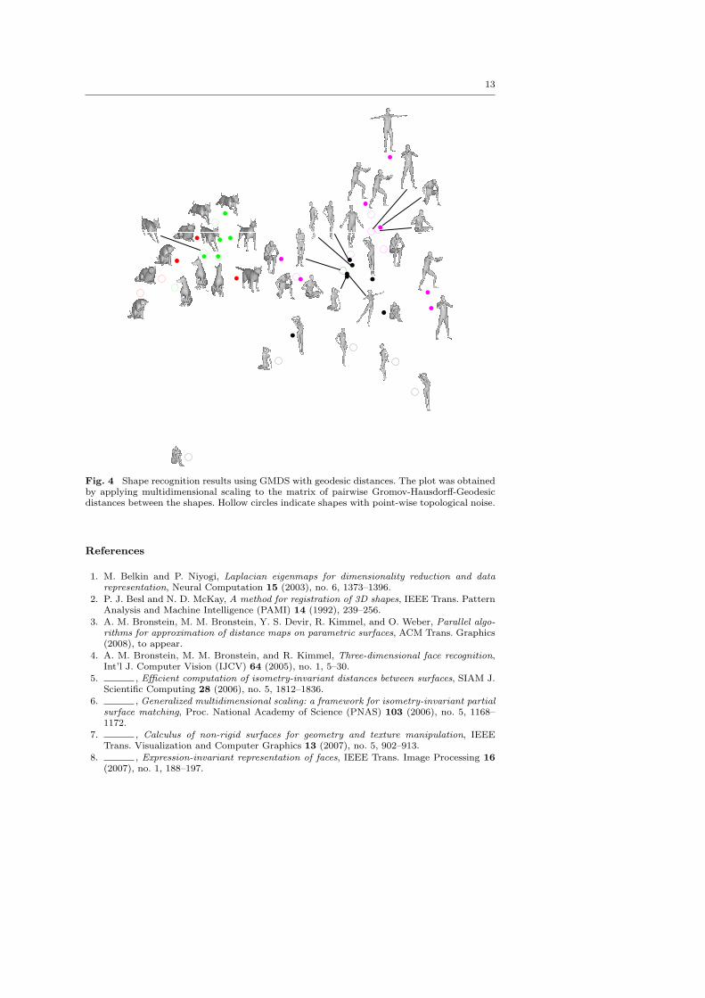
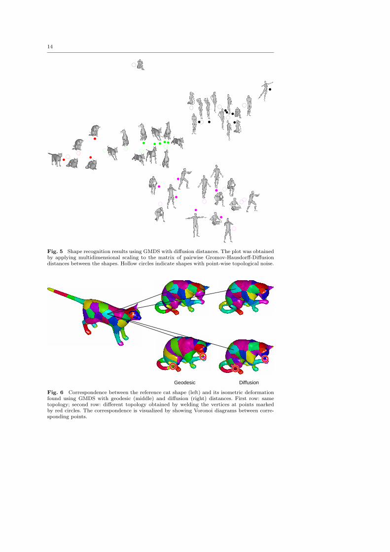
tances, respectively. Figures 4 and 5 visualize the shape similarity with both distances.

Note how the diffusion distance leads to a much clear clustering of the four classes.

Figure 6 shows the correspondence between different deformations of the cat object,

obtained as a byproduct of GMDS with geodesic and diffusion distances, respectively.

To quantify the correspondence quality, we measured the L1 distance between the

computed correspondence C = (P×Q′)∪(Q×P ′) and the groundtruth correspondence

C0 = (P0 ×Q′0) ∪ (Q0 × P ′0), defined as

d(C, C0) =1

2

(‖D(P ′, P ′0)‖1n2 · diam(X)

+‖D(Q′, Q′0)‖1m2 · diam(Y )

),

where the distance matrices D and the diameters are understood in the sense of the

geodesic or the diffusion metrics. The achieved correspondence quality is summarized

in the following table:

Geodesic Diffusion

Without topology changes 0.0514 0.0268

With topology changes 0.1586 0.0291

The correspondence appears to be accurate and satisfactory visually for both distances

when no topological changes are present. However, as the result of topological changes,

the correspondence obtained using geodesic distances deteriorated approximately three

times, whereas the the correspondence computed using diffusion distances deteriorates

by less than 10%.

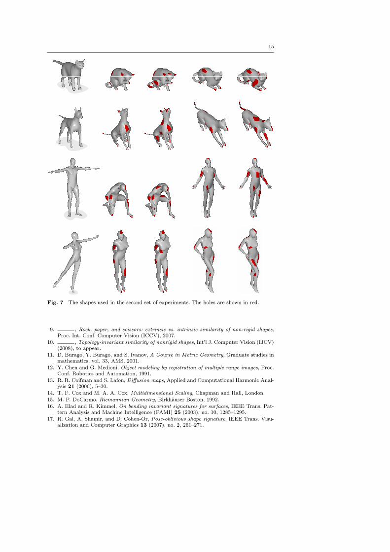
In the second set of experiments, we tested the sensitivity of shape recognition

to holes. Such topological changes are often encountered as acquisition imperfections

when the shapes are acquired using a 3D scanner. We used a subset of the TOSCA

shape database, consisting again of four different objects: cat, dog, male, and female.

Each of the objects had a reference pose and two near-isometric deformations. Each

deformation, in turn, had two versions: with 10 and 20 holes (see Figure 7).

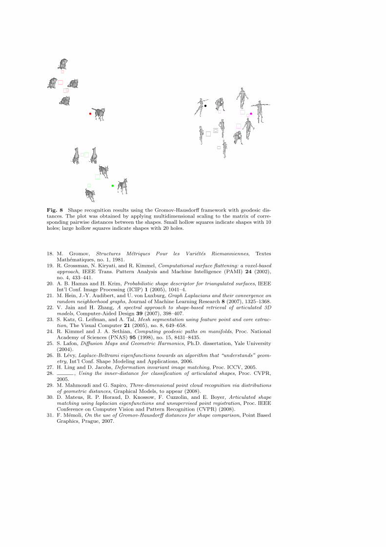
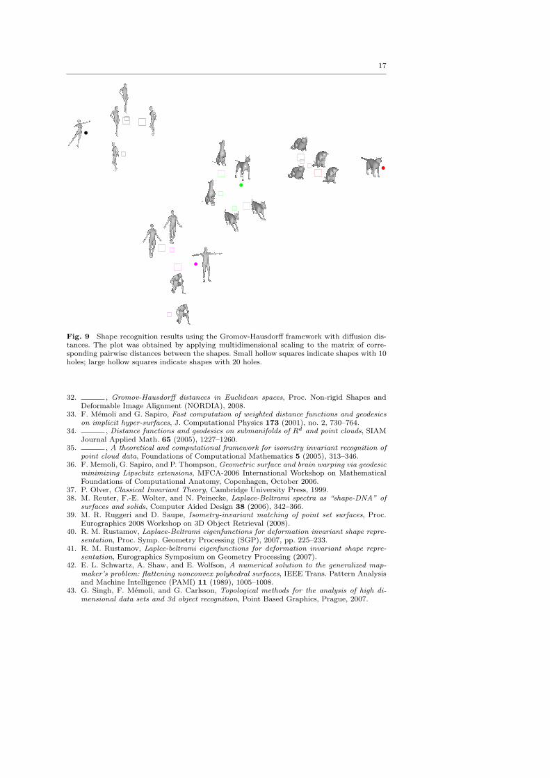
Figures 8 and 9 visualize the shape similarity with both methods. Note for example

how the men and women are much better separated with the diffusion distance. The

EER in this experiment is 0% for diffusion distances and 6.8% for geodesic distances.

11

Fig. 2 The shapes used in the first set of experiments. Red circles indicate point-wise topo-logical changes.

6 Conclusions

In this paper, we addressed the problem of shape recognition in the presence of topo-

logical changes. We used the metric approach, modeling shapes as metric spaces and

posing the problem of shape similarity as the similarity between metric spaces. We

showed that the Gromov-Hausdorff distance, previously applied to geodesic metrics for

bending-invariant shape recognition, can be applied to shapes endowed with diffusion

geometry, leading to a topologically robust approach for non-rigid 3D shape comparison

and matching. In particular, we showed how replacing the geodesic distance between

pair of surface points by the diffusion distance, leads to recognition improvements for

data with topological variations such as holes and connectivity changes. This robust-

ness to holes is a first step toward the recognition of partial shapes, since the missing

portion can be considered as a “hole.”

12

10-3

10-2

10-1

100

10-3

10-2

10-1

100

FAR

FR

R

Diffusion

Geodesic

Fig. 3 ROC curves for the first experiment. The EER is 4% for diffusion distances and 13.5%for geodesic distances.

In addition to the practical consequences brought by the proposed framework, this

work opens the door to moving beyond the classical use of geodesics for intrinsic non-

rigid shape matching. Thereby, the use of other intrinsic distances, as well as other

kernels in the diffusion framework, deserves further study. The combination of such

distances may lead to further performance improvements as well. The combination of

the Gromov-Hausdorff-Diffusion framework with topological features as those described

in [43] is of great practical interest as well.

At a theoretical level, many existing questions are emphasized and new ones are

posed. The geometry of the shape space defined by the Gromov-Hausdorff metric with

diffusion distances is of great theoretical and practical significance. In addition, the

study of the classes of shape transformations under which the diffusion geometry is

invariant (“diffusion isometries”) and their relation to “geodesic isometries” should

give an important insight on the cases in which each of the methods is preferable.

Acknowledgments

GS thanks Dr. Facundo Memoli, Stanford University, with whom the travel into the

Gromov-Hausdorff and metric shape comparison world started.

13

Fig. 4 Shape recognition results using GMDS with geodesic distances. The plot was obtainedby applying multidimensional scaling to the matrix of pairwise Gromov-Hausdorff-Geodesicdistances between the shapes. Hollow circles indicate shapes with point-wise topological noise.

References

1. M. Belkin and P. Niyogi, Laplacian eigenmaps for dimensionality reduction and datarepresentation, Neural Computation 15 (2003), no. 6, 1373–1396.

2. P. J. Besl and N. D. McKay, A method for registration of 3D shapes, IEEE Trans. PatternAnalysis and Machine Intelligence (PAMI) 14 (1992), 239–256.

3. A. M. Bronstein, M. M. Bronstein, Y. S. Devir, R. Kimmel, and O. Weber, Parallel algo-rithms for approximation of distance maps on parametric surfaces, ACM Trans. Graphics(2008), to appear.

4. A. M. Bronstein, M. M. Bronstein, and R. Kimmel, Three-dimensional face recognition,Int’l J. Computer Vision (IJCV) 64 (2005), no. 1, 5–30.

5. , Efficient computation of isometry-invariant distances between surfaces, SIAM J.Scientific Computing 28 (2006), no. 5, 1812–1836.

6. , Generalized multidimensional scaling: a framework for isometry-invariant partialsurface matching, Proc. National Academy of Science (PNAS) 103 (2006), no. 5, 1168–1172.

7. , Calculus of non-rigid surfaces for geometry and texture manipulation, IEEETrans. Visualization and Computer Graphics 13 (2007), no. 5, 902–913.

8. , Expression-invariant representation of faces, IEEE Trans. Image Processing 16(2007), no. 1, 188–197.

14

Fig. 5 Shape recognition results using GMDS with diffusion distances. The plot was obtainedby applying multidimensional scaling to the matrix of pairwise Gromov-Hausdorff-Diffusiondistances between the shapes. Hollow circles indicate shapes with point-wise topological noise.

Geodesic Diffusion

Fig. 6 Correspondence between the reference cat shape (left) and its isometric deformationfound using GMDS with geodesic (middle) and diffusion (right) distances. First row: sametopology; second row: different topology obtained by welding the vertices at points markedby red circles. The correspondence is visualized by showing Voronoi diagrams between corre-sponding points.

15

Fig. 7 The shapes used in the second set of experiments. The holes are shown in red.

9. , Rock, paper, and scissors: extrinsic vs. intrinsic similarity of non-rigid shapes,Proc. Int. Conf. Computer Vision (ICCV), 2007.

10. , Topology-invariant similarity of nonrigid shapes, Int’l J. Computer Vision (IJCV)(2008), to appear.

11. D. Burago, Y. Burago, and S. Ivanov, A Course in Metric Geometry, Graduate studies inmathematics, vol. 33, AMS, 2001.

12. Y. Chen and G. Medioni, Object modeling by registration of multiple range images, Proc.Conf. Robotics and Automation, 1991.

13. R. R. Coifman and S. Lafon, Diffusion maps, Applied and Computational Harmonic Anal-ysis 21 (2006), 5–30.

14. T. F. Cox and M. A. A. Cox, Multidimensional Scaling, Chapman and Hall, London.

15. M. P. DoCarmo, Riemannian Geometry, Birkhauser Boston, 1992.

16. A. Elad and R. Kimmel, On bending invariant signatures for surfaces, IEEE Trans. Pat-tern Analysis and Machine Intelligence (PAMI) 25 (2003), no. 10, 1285–1295.

17. R. Gal, A. Shamir, and D. Cohen-Or, Pose-oblivious shape signature, IEEE Trans. Visu-alization and Computer Graphics 13 (2007), no. 2, 261–271.

16

Fig. 8 Shape recognition results using the Gromov-Hausdorff framework with geodesic dis-tances. The plot was obtained by applying multidimensional scaling to the matrix of corre-sponding pairwise distances between the shapes. Small hollow squares indicate shapes with 10holes; large hollow squares indicate shapes with 20 holes.

18. M. Gromov, Structures Metriques Pour les Varietes Riemanniennes, TextesMathematiques, no. 1, 1981.

19. R. Grossman, N. Kiryati, and R. Kimmel, Computational surface flattening: a voxel-basedapproach, IEEE Trans. Pattern Analysis and Machine Intelligence (PAMI) 24 (2002),no. 4, 433–441.

20. A. B. Hamza and H. Krim, Probabilistic shape descriptor for triangulated surfaces, IEEEInt’l Conf. Image Processing (ICIP) 1 (2005), 1041–4.

21. M. Hein, J.-Y. Audibert, and U. von Luxburg, Graph Laplacians and their convergence onrandom neighborhood graphs, Journal of Machine Learning Research 8 (2007), 1325–1368.

22. V. Jain and H. Zhang, A spectral approach to shape-based retrieval of articulated 3Dmodels, Computer-Aided Design 39 (2007), 398–407.

23. S. Katz, G. Leifman, and A. Tal, Mesh segmentation using feature point and core extrac-tion, The Visual Computer 21 (2005), no. 8, 649–658.

24. R. Kimmel and J. A. Sethian, Computing geodesic paths on manifolds, Proc. NationalAcademy of Sciences (PNAS) 95 (1998), no. 15, 8431–8435.

25. S. Lafon, Diffusion Maps and Geometric Harmonics, Ph.D. dissertation, Yale University(2004).

26. B. Levy, Laplace-Beltrami eigenfunctions towards an algorithm that “understands” geom-etry, Int’l Conf. Shape Modeling and Applications, 2006.

27. H. Ling and D. Jacobs, Deformation invariant image matching, Proc. ICCV, 2005.28. , Using the inner-distance for classification of articulated shapes, Proc. CVPR,

2005.29. M. Mahmoudi and G. Sapiro, Three-dimensional point cloud recognition via distributions

of geometric distances, Graphical Models, to appear (2008).30. D. Mateus, R. P. Horaud, D. Knossow, F. Cuzzolin, and E. Boyer, Articulated shape

matching using laplacian eigenfunctions and unsupervised point registration, Proc. IEEEConference on Computer Vision and Pattern Recognition (CVPR) (2008).

31. F. Memoli, On the use of Gromov-Hausdorff distances for shape comparison, Point BasedGraphics, Prague, 2007.

17

Fig. 9 Shape recognition results using the Gromov-Hausdorff framework with diffusion dis-tances. The plot was obtained by applying multidimensional scaling to the matrix of corre-sponding pairwise distances between the shapes. Small hollow squares indicate shapes with 10holes; large hollow squares indicate shapes with 20 holes.

32. , Gromov-Hausdorff distances in Euclidean spaces, Proc. Non-rigid Shapes andDeformable Image Alignment (NORDIA), 2008.

33. F. Memoli and G. Sapiro, Fast computation of weighted distance functions and geodesicson implicit hyper-surfaces, J. Computational Physics 173 (2001), no. 2, 730–764.

34. , Distance functions and geodesics on submanifolds of Rd and point clouds, SIAMJournal Applied Math. 65 (2005), 1227–1260.

35. , A theoretical and computational framework for isometry invariant recognition ofpoint cloud data, Foundations of Computational Mathematics 5 (2005), 313–346.

36. F. Memoli, G. Sapiro, and P. Thompson, Geometric surface and brain warping via geodesicminimizing Lipschitz extensions, MFCA-2006 International Workshop on MathematicalFoundations of Computational Anatomy, Copenhagen, October 2006.

37. P. Olver, Classical Invariant Theory, Cambridge University Press, 1999.38. M. Reuter, F.-E. Wolter, and N. Peinecke, Laplace-Beltrami spectra as “shape-DNA” of

surfaces and solids, Computer Aided Design 38 (2006), 342–366.39. M. R. Ruggeri and D. Saupe, Isometry-invariant matching of point set surfaces, Proc.

Eurographics 2008 Workshop on 3D Object Retrieval (2008).40. R. M. Rustamov, Laplace-Beltrami eigenfunctions for deformation invariant shape repre-

sentation, Proc. Symp. Geometry Processing (SGP), 2007, pp. 225–233.41. R. M. Rustamov, Laplce-beltrami eigenfunctions for deformation invariant shape repre-

sentation, Eurographics Symposium on Geometry Processing (2007).42. E. L. Schwartz, A. Shaw, and E. Wolfson, A numerical solution to the generalized map-

maker’s problem: flattening nonconvex polyhedral surfaces, IEEE Trans. Pattern Analysisand Machine Intelligence (PAMI) 11 (1989), 1005–1008.

43. G. Singh, F. Memoli, and G. Carlsson, Topological methods for the analysis of high di-mensional data sets and 3d object recognition, Point Based Graphics, Prague, 2007.

18

44. A. Spira and R. Kimmel, An efficient solution to the eikonal equation on parametricmanifolds, Interfaces and Free Boundaries 6 (2004), no. 3, 315–327.

45. J. B. Tennenbaum, V. de Silva, and J. C. Langford, A global geometric framework fornonlinear dimensionality reduction, Science 290 (2000), no. 5500, 2319–2323.

46. J. Walter and H. Ritter, On interactive visualization of high-dimensional data using thehyperbolic plane, Proc. Int’l Conf. Knowledge Discovery and Data Mining (KDD), 2002,pp. 123–131.

47. Z. Wood, H. Hoppe, M. Desbrun, and P. Schroder, Removing excess topology from isosur-faces, ACM Transactions on Graphics 23 (2004).

48. L. Yatziv, A. Bartesaghi, and G. Sapiro, O(N) implementation of the fast marching algo-rithm, J. Computational Physics 212 (2006), no. 2, 393–399.

49. G. Zigelman, R. Kimmel, and N. Kiryati, Texture mapping using surface flattening viamulti-dimensional scaling, IEEE Trans. Visualization and Computer Graphics (TVCG) 9(2002), no. 2, 198–207.