1

A Guide for Analysing Electrodermal Activity

(EDA) & Skin Conductance Responses (SCRs)

for Psychological Experiments

(Revised version: 2.0)

{via the Biopac MP36R & AcqKnowledge software}

Dr Jason J Braithwaite {Behavioural Brain Sciences Centre, School of Psychology, University of Birmingham, UK}

Dr Derrick G Watson

{School of Psychology, University of Warwick, UK}

Robert Jones {Linton Instrumentation, UK}

Mickey Rowe {Biopac, USA}

{Technical Report, 2nd version: Selective Attention & Awareness Laboratory (SAAL)

Behavioural Brain Sciences Centre, University of Birmingham, UK}

Revised in 2015©

2

Recommended Reading

Boucsein, W., Fowles, D.C., Grimnes, S., Ben-Shakhar, G., Roth, W.T., Dawson, M.E., & Filion, D.L (2012). Publication recommendations for electrodermal measurements. Psychophysiology, 49, 1017-1034. Boucsein, W (2012) Electrodermal activity (2nd Ed). New York: Springer. Critchley, H.D. (2010). Electrodermal Responses: What Happens in the Brain. The Neuroscientist, 8, 132-144. Dawson, ME, et al (2001) The Electrodermal System. In J. T. Cacioppo, L. G. Tassinary, and G.B. Bernston, (Eds) Handbook of Psychophysiology (2nd Ed), 200–223. Cambridge Press, Cambridge. Venables, PH, & Christie, MJ (1980). Electrodermal activity. In Martin, I & Venables, PH (Eds) Techniques in Psychophysiology, 3-67. Chichester, UK. Wiley. Nagai, Y., Critchley, H.D., Featherstone, E., Trimble, M.R., & Dolan, R.J., (2004). Activity in ventromedial prefrontal cortex covaries with sympathetic skin conductance level: a physiological account of a ‘‘default mode’’ of brain function, NeuroImage, 22, 243-251.

Technology

The Biopac MP36R is a state-of-the-art DAQ device. With specific reference to EDA, it produces exosomatic (DC) measures of skin conductance. It has 4-channels, each of which can be configured to sample up to 100,000samples/sec. It utilises a 24-bit A/D converter making it the fastest sampling and most sensitive device of its type currently available. The device is purely software configured (AcqKnowledge) and has no hardware setting-switches on it (other that the power switch to turn it on). It can be interfaced directly to a computer responsible for stimulus presentation so that EDA correlates of specific stimuli can be tagged and detected or it can be used in a more clinical and ambulatory setting merely gathering EDA measures in response to more general environmental / situational stimulation. All data can be analysed in AcqKnowledge and / or saved in formats of other leading packages for further extended analyses (e.g., Excel, Matlab). The existence of 4-channels means that EDA measurements can be simultaneously complemented by additional psychophysiological measures. Data from the MP36R can also be time-linked to concurrent video recordings, where both can be played-back in concert / parallel. This makes it particularly useful for clinical settings and patient-based neuropsychology. The MP36R can also be used as a 4-channel EEG and multiple devices can be linked together to provide more channels.

3

Electrodermal activity (EDA) is the umbrella term used for defining autonomic changes in the electrical properties of the skin. The most widely studied property is the skin conductance, which can be quantified by applying an electrical potential between two points of skin contact and measuring the resulting current flow between them. The EDA complex includes both background tonic (skin conductance level: SCL) and rapid phasic components (Skin Conductance Responses: SCRs) that result from sympathetic neuronal activity. EDA is arguably the most useful index of changes in sympathetic arousal that are tractable to emotional and cognitive states as it is the only autonomic psychophysiological variable that is not contaminated by parasympathetic activity. EDA has been closely linked to autonomic emotional and cognitive processing, and EDA is a widely used as a sensitive index of emotional processing and sympathetic activity This coupling between cognitive states, arousal, emotion and attention enables EDA to be used as an objective index of emotional states. EDA can also be used to examine implicit emotional responses that may occur without conscious awareness or are beyond cognitive intent (i.e., threat, anticipation, salience, novelty). Recent research has shown that EDA is also a useful indicator of attentional processing per-se, where salient stimuli and resource demanding tasks evoke increased EDA responses. Investigations of EDA have also been used to illuminate wider areas of enquiry such as; psychopathology, personality disorders, conditioning, and neuropsychology. Recent improvements in technology, methodology and reporting have meant that EDA has become an increasingly important variable in psychological science. These improvements have also led to further refinements in analysis techniques and the methods used for handling EDA data and making it fit for final analysis and interpretation. Such advancements also leave room for some controversies over how EDA should be analysed in given circumstances. This document is designed primarily for use by non-experts in research on EDA. Plenty of methodological papers / volumes and manufacturers manuals exist already but few provide a digestible guide of how to go from data acquisition to meaningful results in a few basic steps. Here we present a brief guide for EDA analysis with Biopac systems and software (AcqKnowledge). The analyses described here were carried out in AcqKnowledge 4.1. As of the time of writing, all instructions given in this document are valid for this version of the software and will also apply to newer releases as well (though some slight changes should be expected with newer releases). The guide is intended to act as a primer, to get researchers up and running quickly and easily in terms of EDA protocols and analyses with the following assumptions; (i) here we outline the concepts mapped into the framework of the actual software, and (ii) in the knowledge that non-experts will soon become experts by linking the material here to far more extensive discussions. We have tried to keep the guide brief and user-friendly although we strongly recommend it is read in conjunction with additional reading and the Biopac manual. This document has contributions from researchers and members of Biopac and the UK Biopac representatives (Linton Instrumentation). This is a revised document relative to the 1st one we produced (this is version 2.0).

Section 1.1: Background

4

Units

The typical units of electrodermal activity are (i) the microsiemens (µS) or (ii) the micromho

(µmho). Both units are equivalent. So 1µS is equal to 1µmho.

Table 1. Basic definitions for Electrodermal components (adapted from Dawson et al,

2001).

Measure Definition

Skin conductance level (SCL)

Tonic level of electrical conductivity of skin

Skin conductance response (SCR)

Phasic change in electrical conductivity of skin

Non-specific SCR (NS-SCRs)

SCRs that occur in the absence of an identifiable eliciting stimuli

Frequency of NS-SCRs Rate of NS-SCRs that occur in the absence of identifiable stimuli over time

Event-related SCR (ER-SCR)

SCRs that can be attributed to a specific eliciting stimuli

There are two main components to the overall complex referred to as EDA. One component

is the general tonic-level EDA which relates to the slower acting components and

background characteristics of the signal (the overall level, slow climbing, slow declinations

over time). The most common measure of this component is the Skin Conductance Level

(SCL) and changes in the SCL are thought to reflect general changes in autonomic arousal.

The other component is the phasic component and this refers to the faster changing

elements of the signal - the Skin Conductance Response (SCR). Recent evidence suggests

that both components are important and may rely on different neural mechanisms (Dawson

et al., 2001; Nagai et al., 2004). Crucially, it is important to be aware that the phasic SCR,

which often receives the most interest, only makes up a small proportion of the overall EDA

complex.

Electrodermal Activity

(EDA)

Tonic

EDA

Slow changes

&

DC components

Skin Conductance Level

(SCL)

Phasic

SCRs

Non-specific SCRs

(NS-SCRs)

Event-related SCRs

ER-SCRs

Section 1.2: Terms & Definitions

5

It is important to recognise that the tonic EDA (also known as the SCL) generates a

constantly moving baseline. In other words, the background Tonic SCL is constantly

changing within an individual, and can differ markedly between them. This has led some

researchers to conclude that the actual SCL level is not, on its own, that informative or even

that easy to derive (Boucsein, 2012). Simply averaging across the whole signal is woefully

inadequate as a measure of SCL because it likely to over-estimate the true-SCL as such

averages will also contain SCRs (thus artificially elevating the measure). In addition, it is not

clear if any given overall SCL measured in this way can be seen as being 'high' or 'low' for

that individual. At the very least, the researcher should seek to subtract the amplitudes of

SCRs from the Tonic signal before establishing a truer representation of background SCL, or

take measurements from periods outside of SCRs in the signal. In addition, a common

procedure is to devise conditions that can be subtracted from each other - so that the

resultant SCL measure is a relative difference across manipulations (within the individual),

and not based on the absolute numbers, which, as noted above - might not be that

informative. The subtraction procedure acts as a form of normalization for the participant's

EDA data. Further measures of background tonic skin conductance have been suggested -

namely the frequency of NS-SCRs (typically 1-3 per/min during rest and over 20 per/min in

high arousal situations) and the amplitude of these peaks (see Boucsein, 2012)1. These

components are more straightforward to compute - though it is important to use a fixed time-

period of measurement when concentrating on the frequency of the peaks and the

amplitudes of them across conditions and participants2. There is some debate as to whether

counting the frequency / amplitudes of NS-SCRs can be used as a direct replacement for a

measure of more traditional SCL (Boucsein, 2012). This is based primarily on some

observations (mainly in older literature) that SCL can drop as the frequency of NS-SCRs

increases. However, significant increases in the frequency of NS-SCRs are also commonly

seen in high arousal situations and as such can be seen, at the very least, as one indicator of

background arousal. Analysing the amplitudes of NS-SCRs and the standard deviation of

them could also provide additional indicators of tonic arousal. The best way to think about

these issues is that they all provide a valid indication of background tonic processes and

tonic arousal - though are not replacements for each other as a measures of tonic processes.

Note - the detection of NS-SCRs will be affected by the settings in the EDA 'Preferences'

menu. In addition, under high arousal situations it is more likely that NS-SCRs will be

overlapping and occurring in close succession to each other, making the quantification of the

actual number of NS-SCRs dependent on additional criteria.

1 Note - here and elsewhere in this document the term 'Frequency' refers to the number (count) of SCR peaks elicited either as

a function of a given time period (NS-SCRs), or relative to the number of stimulus presentations (ER-SCRs). 2 Obviously if one does not match the time periods one creates a situation where more or fewer peaks can occur in certain

conditions - but this has more to do with unequal time periods not allowing for matched levels to be quantified rather than being due to any real differences in the frequency of NS-SCRs.

Section 1.3: Methodological Issues with Quantifying Tonic EDA / SCL

6

Also within the output for the "Event-Related EDA" routine (discussed later) in

AcqKnowledge, is a value termed 'SCL'. This is not a signal-wide average, but the SCL

value at the time a stimulus was presented (and before the resultant ER-SCR is produced).

It might be possible, in some circumstances, to average across numerous instances of these

SCL values to get a measure of the tonic background periods in between the SCR peaks.

The accuracy of this measure would be improved in circumstances where; (i) these SCL

values occurred outside of previous SCRs; and, (ii) the frequency of ER-SCRs was at or near

100%. This is important because each event in a given signal would provide an SCL value

from which to compute an overall average. As such, one needs to ensure roughly equal

individual SCL observations occur so that the averages are based on a similar number of

observations. If the Frequency of SCRs is vastly different across conditions - then this route

is not advisable because the number of observations contributing to the final SCL values

would be unmatched across conditions. Nevertheless, this is one way that the existing

software could provide values which can be used to navigate around conceptual issues with

EDA research. Another method for delineating a measure of the SCL might involve the "Find

Cycle" routine (discussed later) where the user specifies a time period (say 0.25 seconds)

before every SCR - as this also gives a measure of the tonic SCL which is likely to be outside

of the SCR. Again, one problem here is that the number of observations underlying any

average would be dictated by the number of SCRs present in the signal. This may not be

matched across conditions or participants.

A general friction that has to be balanced in any experiment seeking to measure EDA is

determining a-priori whether a given SCR is event-related or non-specific. If the criteria are

too loose, one risks including NS-SCRs into the analysis for ER-SCRs and erroneously

thinking that such values might be tied to the experimental manipulation. Too strict and one

risks missing many ER-SCRs to meet your criteria by wrongly discarding or misclassifying

them as NS-SCRs. A graphical representation of the components of an ER-SCR is provided

below.

An example of the components of an ER-SCR (taken from Dawson et al., 2001).

Section 1.4: Methodological Issues with Quantifying Phasic ER-SCRs

7

Experimental design and pilot experiments to ascertain the responsive characteristics of EDA

in certain experimental conditions can be useful here to help set these criteria - however,

general guidelines exist that appear satisfactory for most computer-based event-related

experiments.

Latency - Typically an ER-SCR is defined as an SCR whose latency period between

stimulus onset and the first significant deviation in the signal is between 1-3secs. Deflections

in the signal that occur before this period are typically defined as NS-SCRs and are not

viewed as coming directly from experimental manipulations.

Note: In the Event-related EDA analysis menu an option for the "Minimum separation

between Stimulus Event and SCR" is provided. The value entered here is the latency (thus,

the measured time difference that must be greater than this minimum = latency).

Note: Also in the same menu is an option for "Maximum separation between Stimulus

Event and SCR".

Both measures together provide a time "window" for identifying event-related SCRs. If the

measured latency between a stimulus and an SCR is within this window, then that SCR is an

ER-SCR."

Threshold - Historically the most common threshold was set at 0.05µS (approximately the

smallest shift visible on paper chart recorders). However, more recent advances in

technology and precision have led to thresholds of 0.04µS, 0.03µS and 0.01µS becoming

more common in the literature. Deflections in the signal that do not satisfy the threshold

criteria are not counted as SCRs or NS-SCRs.

The importance of visual analysis An initial visual analysis is crucial for all forms of signal analysis and should not be over-

looked because certain factors that were not predicted might be present in the data. For

example, it is common to correct general drift that may appear in SCL data. However,

periodic shifts in the background SCL (i.e., analogous to a DC shift) could be important if

they appear to occur in conjunction with specific components of the experiment. Only a

visual analysis would reveal the initial difference between unimportant drift factors (artefacts)

and potentially important periodic shifts in the tonic background SCL.

Typical values for SCL and SCRs

Although individuals and experimental situations vary considerably, some very general

estimations of 'typical' strength values can be provided. In terms of phasic SCRs, amplitudes

can typically range from threshold to a maximum of around 2-3uS ( X = 0.30uS - 1.30uS: raw

scores, non-normalized) and around 0.20 - 0.60uS on average when logarithmized. In

experiments where highly aversive / threatening / fearful stimuli are used, this maximum

response can increase to around 8uS (non-normalized), but this is rare. Estimations for the

Frequency of NS-SCRs are difficult, but an average of 1-3 per/min (with around 10 per/min

being possible during periods of quietness) has been suggested. High arousal is associated

with around 20-25 per/min (Boucsein, 2012). For SCL, a range of 1-40uS has been

mentioned (Venables & Christie, 1980) though averages are more likely between 2 -16uS.

8

These numbers can be influenced by the size of electrodes and this should be noted in all

scientific reporting.

Acquisition rates: Any digital recording of an analog signal is composed of samples

acquired at discrete time points. Most A/D converters acquire samples at regular intervals.

The timing can be described by that inter-sample interval, or by its reciprocal, the number of

samples acquired per unit time. This sample rate can be set quite low for long-term

ambulatory measurements or experiments that do not require a high level of temporal

precision (i.e., 1-5 samples per second). However, if the researcher wants to run an event-

related analysis - where significant deflections in the EDA signal need to be precise and tied

to stimulus presentations on a computer screen, then 1msec accuracy is required. Lower

sample rates cannot ensure this trigger event is accurately represented in the measurements

and a degree of timing error might occur3. To avoid this, we recommend the acquisition rate

be set to a minimum of 2000 samps/sec (2KHz). This will equate to two samples per-

millisecond thus ensuring 1msec accuracy between the computer presenting the stimulus

(via presentation packages like E-prime) and the trigger sent to the computer recording the

EDA. Note - acquisition rates have implications for the individual channel sample rates

(discussed below) that will be available to the operator. It is up to the operator to ensure that

the acquisition rates implemented allow for the appropriate channel sample rates for the

desired psychophysiological measures.

Channel sample rates: Although EDA is often regarded as a 'slow' measure - it is important

not to fall into the trap of thinking that this means a low sample rate is all that is needed.

Higher sample rates are useful for a number of methodological reasons and for

improvements in precision. The Nyquist theorem would require sampling at twice the

maximum frequency of expected events. For EDA it is typical to filter the data at 35Hz and

so this would represent a theoretical maximum frequency. Therefore, some might argue a

sample rate of 70samples/sec is all that is required. However, the Nyquist theorem is not the

only factor one should consider when selecting an appropriate sample rate. For example,

some recommendations are that a sample rate of 200Hz - 400Hz are a minimum to ensure

enough samples for accurate separation of phasic waveforms from tonic signals (Figner &

Murphy, in press) and a more accurate representation of signal shape. If the researcher is

interested in exploring both factors independently - then sample rates in these regions are

considered a minimum. Recently, modern algorithms for delineating and separating phasic

components from each other (if they happen in close succession) are better satisfied by a

higher sampling of the signal (i.e., deconvolution / negative deconvolution methods), as are

calculations for areas under the curve. So the intended analysis must also be taken into

account when deciding on sample rates. Furthermore, sometimes it is necessary to smooth

a signal due to factors such as noise, sudden deflections, etc. However, some signal

smoothing algorithms require down-sampling. Such down-sampling is always going to be

3 It is up to the individual experimenter to decide for themselves if any given level of error is tolerable and

insufficient to impact on their own data set.

Section 1.5: Methodological tips for Reliable EDA Measurements

9

restricted if the original sample rate was itself quite low. With high sample rates one can

remove a host of artefacts without altering the signal shape markedly and still have plenty of

samples remaining for an appropriate analysis (the ideal scenario). As a consequence of

these observations, a general approach is to always err on the side of caution and probably

seek to sample higher than you really need. The old adage is that the researcher can always

remove samples if they have too many, but you can never put samples into the signal if they

were not there originally. As a general guide, in our laboratory we have sampled EDA at

1000Hz, 2000Hz and 5000Hz to explore signal integrity under a variety of experimental

conditions. The latter is excessive and provides little obvious advantage over both lower

sample rates. As a general rule 500Hz - 2000Hz sample rates are more than sufficient for

laboratory studies and easily achievable for contemporary devices like the MP36R.

Laptops / computers for driving DAQ devices

The Biopac MP36R interfaces to a computer via a USB cable - which can support the high

throughput of data that the DAQ device is capable of producing (in principle). However, we

recommend that researchers spend some time ensuring the computers they use to drive

such DAQ devices have good rates of data transfer, high memory (for the larger files) and

high RAM size. It is good practice to ensure that the computer configuration is not

hampering the ability of the MP36R to operate in an optimal manner. It is the responsibility

of researchers themselves to ensure that this is the case. In our lab (University of

Birmingham), our MP36R is interfaced to a HP power-elite pro-book laptop with a 2.2GB

Quadro graphics card, this configuration provides a highly efficient and effective measuring

system with smooth real-time data graph scrolling and no data loss. This configuration has

been tested at the limits of the capabilities of the MP36R (high data transfer, high gain,

multiple channels running simultaneously, long-term measuring) - with no noticeable issues.

The MP36R is limited primarily by the capacity of the computer operating it - so these

decisions are important.

Top tip: = It is often good practice to run a baseline measurement period when the

participant is not engaged in any given task. Our recommendation is to use between a 2-min

to 4-min baseline session. Such sessions can also help inform as to whether certain

participants are likely to be hyper or hypo-responders independent of any effects of

psychological manipulation. From this, the researcher can measure the frequency of NS-

SCRs (as a measure of EDA responsiveness in the tonic SCL), the average amplitude of

these NS-SCRs, and the SCL before experimentation.4

Top Tip: = In addition to any baseline conditions the experimenter may use, it is

advisable that one allows for a baseline period within any given experimental signal. This

can be (i) at the beginning of the signal recording, at the end, or both. We recommend a

60sec (minimum) period be provided within any given signal and it is more commonplace to

assign this period to the beginning of the measurement period. The purpose of this period is

to facilitate the calculations the software needs to make. Some routines require a moving

window to pass through the signal to make calculations, and it is from these calculations that

accurate deviations can be established. The integrity of this process is optimised if a

4 Though see the earlier section on the problems surrounding SCL quantification.

10

sufficient baseline period is provided within the signal being analysed. In addition, it provides

a baseline SCL measurement right at the time leading up to, and just before, the very start of

the experiment.

There is considerable confusion in the field surrounding the procedures of Normalization and

Standardization. These are not the same thing. Normalization refers to data transformations

to correct for skew / kurtosis so that the data are fit for parametric statistical analysis.

Normalization does not help with between-participant differences / comparisons.

Standardization refers to correcting the data so that they can be directly and meaningfully

compared between individuals. Many researchers confuse these issues and / or do not carry

out standardization procedures when perhaps they should. Standardization may not always

be necessary, but it is difficult to think of a scenario where it might not a prudent idea to

transform any SCRs from an individual, into a co-ordinate system that reflects the limitations

of their capacity to respond per-se. The purpose of standardization is to facilitate individual-

difference comparisons where all SCRs have been transformed, relative to their physiological

responsiveness, and thus to factor out issues like thickness of skin, etc. In principle this is no

different to the neurophysiologist wanting to compare individual differences in Event-Related

Potentials (ERPs) but where the thickness of the skull, air-gap between brain and skull, and

sensor position etc, may all vary slightly.

Some components of EDA may require transformation before they can be analysed formally.

This is based on the fact that the SCL and SCRs can be non-normally distributed and can

display signs of skew and kurtosis. It is advised that all data-sets are explored for measures

of skew, kurtosis, and heterogeneity of variance before formal analysis is carried out. If

these dimensions are satisfactory then no normalization corrections need to be applied.

If normalization transformations are required, the following are typical of the field (see

Boucsein, 2012; Dawson et al., 2001).

SCL measurements - can be corrected by taking the Log of the scores, applied after the amplitudes have been determined (not by applying the log to the raw scores). They can also be transformed via square-root transformations. SCR amplitude measurements - can be corrected by applying a square-root transformation to the SCR amplitudes, which does not require the inclusion of a constant. One can also take the Log of the scores - again, applied after the amplitudes have been determined (not by applying the log to the raw scores). SCR magnitude measurements - where zero responses are included, a 1 is added to all SCR amplitudes before the log is performed (Log (SCR +1) because the logarithm of zero is not defined. Ultimately, Log transformations or Square Root Transformations are applied as corrections - and both produce roughly comparable results. The aim here is to make the data fit for the assumptions of parametric analysis. Although rare, if these transformations are not sufficient to correct the distribution of measurements, then non-parametric statistics should be used.

Section 1.6: Data Transformations: Normalizations & Standardizations

11

On occasion the researcher might want to transform their SCR / SCL data into a

standardised and corrected form (to correct for inter-individual variance) that can facilitate an

individual-difference analysis. There is no universally agreed on method for this and there

are pros and cons to every procedure. A number of suggestions have been made and used

in the literature and their utility is still being debated. The most common are as follows:

SCL data: Range-Corrected Scores: Here one computes the minimum SCL during a

baseline or rest period and a maximum SCL during the most arousing period. The

participants SCL at any other time period in the study can then be delineated as a proportion

/ percentage of their individual maximum range of psychophysiological response via the

formula (SCL - SCLmin) / (SCLmax - SCLmin: Dawson et al., 2001).

SCR data: Proportion of Maximal Response: In the case of SCR data, we can assume

the minimum to be zero and the maximum to be the result of a startle stimulus (i,e.,

surprising white noise stimuli played through earphones, hand-clap, balloon pop, and / or

taking deep breaths). From this, each individual SCR can then be standardised for individual

differences by dividing it by the participants maximum SCR.

One issue with these approaches is that what counts as 'minimum' can be artificially

constrained by the technology and not necessarily represent the true minimum SCL / SCR.

It is also difficult to ensure that the startle response is indeed a reliable indicator of maximum

response. Furthermore, startle responses are not consistent, even within the same

individual, and range correction procedures are problematic if different groups have very

different ranges (Ben-Shakhar, 1985; Dawson et al., 2001). As a consequence, these

methods outlined above have become increasingly controversial.

Transformations into standard values: Some studies recommend transforming SCRs into

Z-scores (Ben-Shakhar, 1985). This requires the mean and standard-deviation to be used

instead of a hypothetical maximum (from the other methods above). This navigates around

the problems associated with determining the maximum SCR response from range-corrected

methods / maximal correction methods. Here each raw SCR, a mean SCR value and

standard deviation of SCRs, are used to compute the Z-score which is normally distributed,

has an average of 0 and a standard deviation of 1. From here one can transform these Z-

scores into T-scores, which have a mean of 50 and standard deviation of 10 (thus removing

minus scores: see Boucsein, 2012). The advantage to this approach here is that the

resultant z-scores are based on unambiguous mathematical factors that represent the

participants typical response level and not on unwarranted assumptions about maximum

SCRs. In response to other views, Ben-Shakhar, (1987) further suggested that another

useful transformation might be to divide each raw SCR, by the participants mean SCR thus

providing a kind of 'standardised ratio'. Note, although not explicitly stated in the paper, Ben-

Section 1.7: Standardizations for Individual Differences

12

Shakhar (1985) appears to be suggesting that z-score transformations are for measures of

SCR amplitude (as no mention of applying the Log(SCR + 1) for magnitudes correction is

given). However, we see no reason why this could not equally apply to measures of SCR

magnitude.

Correcting for drift in SCL

An important artefact to control for in EDA research is that of 'drift' in the background SCL.

This is really more of a problem with long experiments and / or long-term ambulatory

monitoring. In terms of a visual analysis of the signal, one will see what appears to be a

general climbing in the background Tonic SCL. The issue of how to determine whether such

shifts are artefacts (drift) or important shifts in real tonic processes is not an easy one to

solve. However, some general points are worth noting. First, all SCRs identified in the

Acqknowledge software are delta functions between the onset of the SCR and the peak

SCR. In this sense, all SCRs are normalised to the immediate SCL context (the onset) and

as such, the impact of drift is largely removed. The resulting SCR tends to be 'blind' to the

overall SCL (in many cases). In extreme cases excessive drift can impact on the measured

amplitude of SCRs (greater drift = lower SCRs) due to the move towards ceiling values.

Controlling for drift is good experimental practice and will impact on assessments of tonic

SCL and the accurate identification of important shifts in tonic processes. Second, drift can

be controlled for by the implementation of: (i) separate baseline screening sessions: (ii) a

baseline period at the start of each experiment occurring within the main experimental signal

(as discussed above) and: (iii) the use of periodic rest periods within the experiment to be

used as calibration points (which can be used to carry out a linear interpolation on the

signal). In a general sense the artefact of drift takes more time to accrue than more localised

and potentially important shifts in the DC background tonic SCL. Localised shifts in tonic

SCL can manifest themselves within a few tens of seconds whereas drift may take many

tens of minutes to become apparent. Nevertheless, the presence of drift could potentially

mask true shifts in emotional processing indexed by localised shifts in tonic SCL.

13

Setting the Acquisition rate

Step 1 - Select MP36, and select 'Set Up acquisition'. From here you can select an

appropriate digital sample rate and whether to save the data file to RAM or Disc memory (the

capacity is limited by the computer hardware).

Note: - the acquisition rate will have implications for setting up individual channel sample

rates as these are derived from the overall acquisition rate. If setting up multiple channels -

then it is important to ensure that the acquisition rate is high enough to satisfy all channel

requirements.

Section 2.0: Setting up

14

Setting up a basic channel for EDA recordings

Step 1 - Go to the main menu - select MP36 - and select Set Up channels.

Step 2 - CH1 - Under the drop-down menu for 'preset' select Electrodermal Activity (EDA) 0-

35Hz. Then go to the 'Setup' icon. From here you can set the required gain settings. (leave

the other settings for the filters etc unaltered as they are set for standard EDA protocols and

would only require altering for specific aims). The choice of gain is down to the individual

researcher - though x1000 is perfectly fine. We have run experiments with x2000 and x5000

levels of gain - both work well, but note that the higher the gain then the lower the dynamic

range. Therefore, deciding on an appropriate gain level is a decision requiring a trade-off

between gain and range. We recommend x1000 / x 2000 as being more than sufficient for

most purposes and represents a good balance between gain and range.

15

Set the gain here (above).

A major advantage of the MP36R is that it is purely configured by software and these

settings can be saved as a 'Template' file (under the save-as menu drop-down bar) and

easily opened up for recording consistent measurements. Having no hardware switches

eliminates the possibility that switches and settings can be changed accidentally by multiple

operators and for error creeping into acquisition5. Once configured, the operator simply

needs to open the template file and re-save it under a different name as a Graph file and all

these settings will be automatically applied for immediate measurement.

In our laboratory we currently gather EDA measurements at the higher-end of the necessary

specifications. We know that the following settings give high-quality EDA data suitable for

post-acquisition filtering / smoothing while maintaining the integrity of the measurements.

The final decision rests with the individual researcher and the needs / duration of the

experiment. For reference, our generic settings are (for an experiment lasting approx

60mins);

EDA channel sample rate = 2KHz (2000 samps/sec). Acquisition sampling rate = 500 - 2000samples/sec. Gain = x1000 / x2000. These settings can be limited by the computer hardware linked to the MP36R and an indication of the file size is given when stepping through these procedures.

5 This is a major advantage for teaching as well as research, as the tutor can simply set up templates for the students to

adopt and be confident that consistent settings are being applied across participants.

16

Getting started (i)

Any analysis of a time-series signal begins with a visual inspection of the signal. Here the

observer is looking at the overall characteristics and examining the integrity of the signal.

This is best achieved by both examining the overall signal in the window (if the signal is not

too long) and also zooming into the signal and moving through it in stages from start to finish.

Crucially one is inspecting the signal for artefacts such as periods of poor contact or sharp

square-wave spiking that may reflect contamination from an artificial source. These artefacts

can be removed easily in a number of ways. Perhaps the simplest way of smoothing out and

removing these artefacts is to down-sample the signal by a given constant (Transform >

Smoothing > Samples). Care should be taken that the constant is sufficient to ensure a

desired amount of smoothing without being so excessive as to distort the signal shape. On

rare occasions noise / artefacts can be too excessive and so the data should be discarded.

Getting Started (ii)

Assuming the operator wants to carry out a standard EDA analysis (in line with established

protocols in the scientific literature), within the EDA-analysis domain of Biopac's

Acqknowledge software there are three main ways one can approach, explore and analyse

their EDA data. These are: (i) manually via the I-Beam procedure linked to pre-set

measurement box options that the operator can configure in the menu bar: (ii) via a series of

discrete automatic routines under the "Electrodermal activity" option from the "Analysis"

menu and: (iii) the 'Find Cycle' routine under the analysis option. The I-Beam analysis

provides a host of useful values that can be selected by the operator - but this procedure

does not identify significant components within the signal or discriminate between NS-SCRs,

or ER-SCRs. To ascertain this information one needs to access the automatic routines that

are also available. Both of the automatic procedures (the "Locate SCRs" and the "Event-

related EDA analysis") are reliant on the same settings that are established under the

additional "Preferences" option. That is to say, these preferences, once set, stand and

impact on all subsequent automatic EDA routines.

Section 2.1: Analysis: Getting Started

17

Preferences: These can be found under the "Analysis" > "Electrodermal Activity" menus.

Two separate routines are available for establishing the presence of Phasic SCRs from the

background Tonic signal. These routines are; (i) a smoothing baseline removal option and,

(ii) a high-pass filter (0.05Hz). The Baseline estimation window refers to the width of the

moving window for the smoothing baseline removal option (if the baseline estimation option

is selected instead of the filter option). The actual value is at the discretion of the researcher

but will impact on the results (the default value is arbitrary). Note - increasing the width,

increases the sensitivity and produces more SCRs. It is irrelevant if the 0.05Hz high-pass

filter option is selected instead to produce a phasic signal. The SCR threshold has

historically been set at around 0.05µS (a visible deflection in old paper chart recorders).

However, 0.04µS to 0.01µS are not uncommon in the more contemporary literature. Our

current preference for SCR threshold is to use one of about 0.03µS (with a range of 0.01µS -

0.03µS). Setting the threshold to zero and the rejection rate to 10% will closely approximate

the SCR detection algorithm outlined in Kim et al., (2004) Emotion recognition system using

short-term monitoring of physiological signals. Medical & Biological Engineering &

Computing, 42, pp. 419-427. Setting the rejection threshold to 0% will retain all potential

SCRs (none will be rejected).

18

The basic screen display

The measurement boxes & the “I-Beam” tool

The I-Beam tool allows you to highlight specific regions of the signal for analysis. This tool

works in conjunction with the measurement boxes (which provide the output from the region

highlighted by the I-Beam tool), which can be configured to provide specific mathematical

information via their individual drop-down boxes. Once the measurement boxes have been

set to measure the desired values, they can all be saved as a 'pre-set' under the pre-set

menu.

Measurement

boxes

Tonic EDA signal

x-axis = time

Y-axis = µS

microsiem

an

The I-Beam tool

60sec baseline period

Stimulus presentation

The Pre-set menu

19

In order to precisely identify discrete and significant short-term changes in the tonic signal,

AcqKnowledge generates a phasic signal (blue signal) which represents true time-based

changes (based on underlying algorithms and some of the preference settings). This is used

by the software to identify SCRs within the tonic signal (red signal) and place: (i) a signal

onset marker (open bracket): (ii) a peak SCR (water droplet) marker and: (iii) a signal offset

marker (closed bracket). This blue phasic signal is not itself analysed by the user (it is used

by the software). This phasic signal must be present before carrying out an Event-related

analysis. It can be easily derived by selecting the "Derive phasic EDA from tonic" option

from the "Electrodermal Analysis" menu (both under "Analysis"), or by selecting the "Locate

SCRs" option with "construct new" channel selected. The former option generates the

phasic signal and the latter option also does this but, in addition, places SCRs onto the red

tonic signal as well.

Step 1. Deriving the phasic components from the Tonic EDA. This essentially produces a

new de-trended signal that the software uses to delineate the presence of SCRs within the

tonic (red) signal.

Section 2.2: How to Identify the Phasic SCR Components from the Tonic EDA

20

The Tonic EDA is now accompanied by a Phasic signal (blue) providing precise information

on time-based changes in the EDA.

Step 2: Go to "Analysis" > "Electrodermal Activity" > and select the "Locate SCRs" option

from the menu.

21

Step 3. Make sure CH1, EDA is selected as the Tonic EDA channel. If you already have a

phasic channel present (as we do here) this can be selected as the channel from which to

construct SCRs - so select CH2, Phasic as the 'Use channel' option. If the phasic channel

has not been computed, click on 'Construct new' and it will be generated and SCRs placed

on the Tonic signal. Both routes lead to the same outcome.

Step 4. SCRs now displayed on the red (top) Tonic channel.

22

Zoomed into a section of the signal - Each SCR is marked as a blue water droplet. Note, each SCR has an open bracket before it, then the SCR, then a closed bracket. These signify, (i) SCR onset: (ii) Peak SCR: (iii) SCR offset, respectively. Open-brackets = SCR onset Water-droplet = Peak SCR response Closed bracket = SCR offset / end of SCR Blue droplet = an SCR that is significant from its background but not tied to a specific stimulus, typically referred to as, a Non-specific-SCR (NS-SCR).

Note: - As can be seen in the above figures, there is a deflection in the first few seconds

of the phasic signal (to the left of the blue signal). This is an artefact from the application of

the 0.05Hz filter and can be avoided if the operator allows for an approx 30-sec period to

pass before beginning the stimulus delivery procedures of their experiment (this is not

present in later versions of the software).

23

Useful I-beam & measurement box settings:

The measurement boxes contain a number of drop-down options for certain mathematical

operations to be carried out on the data linked to the operation of the I-Beam. These can be

set up and saved as pre-sets - so that they can be applied to every signal loaded into

AcqKnowledge just by clicking on the appropriate pre-set name. Here we describe perhaps

some of the more basic routines and settings that would apply to most EDA experiments.

Mean = returns the arithmetic mean for the whole area highlighted by the I-Beam (averaged

across peaks, troughs, etc).

Value = returns the exact value (level of the signal) at the point where the mouse was last

released.

Standard deviation = provides a standard deviation statistic for the area highlighted by the I-

Beam.

Mean amplitude of events (Evt ampl) = returns the mean of the peak amplitudes only from significant events that have been identified in the area that has been highlighted. Several options are configurable after making this selection. A particularly useful set of options are "Specific SCR" or "Skin Conductance Response" for "Event Type", "Anywhere" for "Location" (the events should be only on the tonic EDA channel, but "anywhere" can be selected so the user does not have to determine which number that channel is), and "Mean amplitude from all events" for "Extract". With these settings, the user can quickly determine the mean of the maximum levels reached by all (specific) SCRs in the highlighted area. This measurement will work as such only after "Locate SCRs" has been run. The resulting number will typically be higher than the basic 'mean' discussed above because only the significant peaks are averaged. Number of events = a count of the number of events of a particular type. As with Evt_ampl..., the type and location of the events to be counted is configurable after this measurement type has been selected. You must have completed a "Find SCR" or equivalent routine first for this to work. This allows for easy measurement of the number of NS-SCRs (for example). Can be set for SCRs or ER-SCRs. Delta = provides a difference value. Particularly useful when used in conjunction with the

"Find cycles" routine. This effectively identifies the SCR when used in this way if the onset

and SCR are defined as start and end events in the "Find cycles" routine. It returns the delta

value between these events - which is equivalent to the output for amplitude in the Event-

related routine.

Tip - to highlight an area that exactly spans, for instance, the time from SCR onset to SCR peak, hold down the Control key while clicking on the open bracket and then hold down the Control key while clicking on the water droplet.

Delta T = provides an accurate time period of the area being highlighted. Allows the

operator to ensure they are highlighting very specific time windows. Is equivalent to "Rise

Time" when used in the "Find Cycles" routine.

Tip - this works more accurately if you zoom into the signal.

24

Min / Max = provides values for the minimum and maximum EDA values encountered in the

highlighted areas and is useful for calculating the range of values. Caution - the minimum

values can be influenced by the sensitivity of the device.

The Event-related EDA analysis" routine is the most comprehensive of the EDA functions

provided. The "derive phasic EDA from Tonic" provides a new phasic signal from the original

tonic EDA which the software then uses for precision time-based changes to be marked

within the tonic signal. The "Locate SCRs" routine identifies all significant (as delineated via

the preferences settings) SCRs from the background signal. However the "Event-related

EDA analysis" routine provides an analysis of the SCRs that match parameters outlined in

Preferences and hence appear to be event-related. These ER-SCRs are coded in

AcqKnowledge as red-droplets with a flag on top. In addition, this routine provides a host of

values including; (i) the Latency of the ER-SCRs (ii) the Skin Conductance Level (SCL); (iii)

Amplitude of all ER-SCRs, (iv) size of ER-SCRs, (v), the Rise Time of ER-SCRs, (vi) ER-

SCR onset, (vii) the Magnitude of the ER-SCRs, and (viii) the Frequency of ER-SCRs.

We will first show how to obtain these values from a signal before providing an explicit

account as to how these values are derived within AcqKnowledge.

Go to “Analysis” > "Electrodermal Activity" > “Event-related EDA Analysis”.

In the present case the stimulus delivery icon (light bulb in the event-bar) signifies when the

stimulus was presented. The software will now search for when / where light-bulbs occur

(stimulus presentations) and calculate whether or not the SCRs can be classified as Event-

related (red-droplets) or not (blue droplets). These calculations are influenced by the

Section 2.4: Using the Event-related analysis routine

25

numbers entered into the minimum separation box (between 1 and 3 seconds is typical)

which defines the minimum time period from stimulus presentation to SCR onset to count as

being “event-related”. A similar logic underlies the maximum separation that can occur

before the SCR is no longer counted as being “event-related” (between 8 – 10 seconds is

typical).

Note: - this routine will typically identify the first SCR that occurred after the stimulus

presentation and thus, as long as it is significant from the background signal - then it

becomes defined as being tied to the stimulus presentation. The first SCR may or may not

be the highest peak in the pre-specified time window. This assumption is the most valid - but

note - some researchers report the maximum peak that occurs in a given time window which

might not always be the first SCR in this period. Researchers need to be aware of

differences across the methods and reporting in the literature and be clear on what they need

to analyse / report. If a precise stimulus-delivery paradigm is being used (i.e., computer

triggers sent from a stimulus-presentation protocol to Acqknowledge), then we advise that

the first SCR within the specified window is the most appropriate to report and analyse -

which is exactly what the software computes.

In the options menu under the event-related analysis - define the Tonic EDA as Ch1, and

select CH2 for the phasic EDA. The stimulus-event type needs to be defined and can be

changed - but is typically defined as Stimulus Delivery (tells the software to search for light-

bulb icons as these signify events). The minimum and maximum time settings should be

established and general suggestions are provided in the example - though these depend on

the individual experimental design and the researcher. Click on 'Output events for specific

SCRs'. Then click 'OK'. Any SCR tied to a stimulus presentation will now be classified as a

red-droplet (ER-SCR). Make sure you set (under preferences) the procedure to also

produce an Excel (or text) file detailing the results of the event-related analysis.

26

Part of the Excel output for the ER-SCRs. As there was only one red-droplet in the signal,

there is only one entry in the data file. This section of the file shows, Time, SCL, Latency,

SCR amplitude, SCR rise time, size, and onset.

Further down in the results file an additional “Magnitude” value and “Frequency” value is also

provided. Note – the term “Frequency” refers to the ratio of (i) how many stimulus

presentations were there in relation to (ii) how many of these presentations resulted in an

ER-SCR. In the present case there was one stimulus presentation and one ER-SCR – so

the Frequency is 100%. In the context of multiple stimulus presentations, the lower the

number = the less reliable the stimuli were in eliciting an ER-SCR.

27

A brief word on amplitude and magnitude

Mean amplitude = mean value computed across only those stimulus presentations that

produced a measurable (i.e., non-zero) response. One problem with the amplitude measure

is that the N used to compute the average response size can vary depending on how many

measurable responses a participant gives (Dawson et al, 2001). So if the experimenter

presents the exact same picture on the computer 5 times, but it only elicits a non-zero

response on three occasions, then the final mean amplitude is the mean of the three

presentations only (sum non-zero amplitudes / number of non-zero responses = amplitude).

The problem here is that a participant who has a response of say, 0.25uS on only one

presentation, will have the same mean amplitude response to a participant who responds

with 0.25uS on all five presentations (see Dawson et al., 2001). Note, as mean amplitudes

are based on non-zero responses, the normalization correction for them does not require a

constant to be added (i.e., use the square-root transformation, not the Log(SCR+1) method).

Mean magnitude = mean value computed across all stimulus presentations including those

without a measurable response (i.e., zero responses). One problem with the mean

magnitude value is that it confounds the frequency of response and the response strength

which do not necessarily co-vary. It is advisable that if magnitude is to be reported - that it is

complemented with a Frequency measure. Note, as mean magnitudes do involve zero

responses, then the normalization correction for them does require a constant to be added

(i.e., use the Log(SCR+1) method)

Note: If you only have one stimulus-specific event in your experiment (as with the

example here) - and it elicits an event-related response, then the amplitude and magnitude

values will be the same. In addition, if your experiment has lots of stimulus presentations

and every stimulus presentation induces an ER-SCR (thus resulting in a red-droplet) - then

the amplitude and magnitude values will also be the same. The values will be different only if

the frequency of ER-SCRs drops below 100%. As a consequence, the frequency is also a

very important value for examining the effectiveness of the stimuli at inducing ER-SCRs.

28

The SCL = I-Beam positioned on Event at 137.7 seconds – which was the time of stimulus presentation (red light-bulb in event bar) and the SCL represents the current value at that time of stimulus presentation. It is important not to confuse the use of this term 'SCL' with that of an SCL value of the whole tonic signal. In the context of the event-related routine here, SCL refers to the background value present in the EDA and the specific time of stimulus presentation only.

SCL value at this time

Stimulus presentation

Section 2.5: What do the Event-related Numbers refer to (or how are they calculated)

29

The Latency = This is the value for the time-period between stimulus presentation and the

onset of the ER-SCR (the area illustrated above under the blue I-Beam region: secs /

msecs).

Latency

Stimulus presentation

30

The SCR amplitude = calculated from the period of the beginning / onset of the SCR (open

bracket) to the peak value within the SCR (µS / µmho). It is essentially a delta function from

SCR onset to the SCR peak as determined by the change in the tonic EDA.

The SCR rise time = The time taken from SCR onset to reach peak amplitude within the

SCR ( number = secs).

The SCR size = Refers to what is, in essence, a peak amplitude. It is the value at the time of

max SCL.

I-beam positioned

at time of max SCL Value at this time

SCR amplitude

SCR rise-time

31

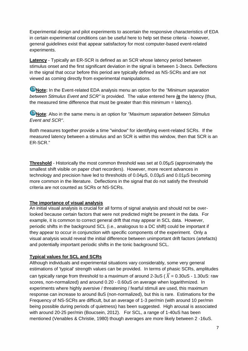
SCR onset = The value (µS / µmho) where the SCL first rises above the pre-set threshold

and this signals the onset of the SCR. This is signified in the data as an open bracket. Note

- if you know the onset value, and you know the peak amplitude (SCR size) you can compute

the actual phasic SCR via a delta function between these values, as SCR is a relative

change to the deflection in the signal from onset to peak response.

Cursor positioned where SCL rises

above threshold

32

A schematic representation of how the event-related analysis routine works through

the signal to identify ER-SCRs

33

Note: - if stimulus events are packed close together this can generate potential errors in

pairing the appropriate event to the appropriate response. Under such circumstances it is

possible that the first SCR after a stimulus delivery will be paired with a previous stimulus

delivery event and that a second SCR may then be judged specific to the stimulus delivery

event.

Note: - to create the above figure, the Stimulus Delivery events labeled "2", "3", and "8" were in the original file. The "Event-related EDA Analysis" routine was run. The result is depicted by the events shown in the bottom channel. This channel was duplicated without the events, the event labeled "57" was added to the events bar, and then the "Event-related EDA Analysis was run again. The result is depicted in the top channel. The second SCR is within the window for events 57 and 8, and could, in principle, have been elicited by either event. In the original analysis (without event 57) this SCR is determined to have been caused by event 8. Once event 57 has been added, it is concluded to have been the event which caused this SCR. When processing event 8, the algorithm looks for another SCR that might be in its window after it has been determined that the first SCR in its window has already been paired with an earlier stimulus event. Event 3 then loses its SCR to event 8 for the same reason. In real terms, event 3 might have been the cause of either or both of the last two SCRs, but the analysis will conclude that it did not elicit any. To avoid situations like this, always ensure a large (relative to the latency window) separation between discrete stimulus delivery events. The above figure was created for illustrative purposes only -- the latency windows were intentionally made long to produce these results using data that were actually acquired with adequate separation between adjacent stimulus delivery events.

Note: - General Point: SCRs can also be induced when stimuli are removed (stimulus

offset) as well as when they are presented. For this reason it is good practice to provide a

sufficient inter-stimulus-interval (ISI) after stimuli have been removed from the previous trial

and before the next stimulus is to be presented. In addition, if possible within an

experimental design, the experimenter could also adopt a faded offset of stimuli.

Analysis run AFTER event 57 was added

Analysis run BEFORE event 57 was added

2 57

8 3

34

An additional method for gleaning the amplitudes (and other variables) from all the significant events in a signal is to employ the "Find Cycle" routine from the "Analysis" menu. This can provide you with an excel spreadsheet containing a number of values that correspond to the events selected and the measures highlighted in the measurement boxes. This routine can also obtain statistics for all skin conductance responses from circumstances when there is no information about the time of stimulus delivery (i.e., ambulatory measurements) or the operator wants to override some of the constraints from the "Event-related" routine.

This procedure allows the user to perform the analysis on a file without markers, as it is possible to place a marker 1 sec (for example) prior to every waveform onset of an SCR and then run the automated analysis with this marker set as the stimulus. In essence this routine allows the user to treat every significant SCR as an ER-SCR. A worked example is provided below.

Go to “Analysis” and select “Find Cycle”. Enter selections in the options as shown above.

Select “events”, the waveform onset as the ‘start event’ – then select the channel on which

the operation is to be carried out (in this case the Tonic channel), then select skin

conductance response as the “end event”. This tells the software to identify cycles from their

onset to their peak SCR and the signal will then have blue marker bars to define these.

Once done – click “Selection”. The differing shades of blue (lighter / darker) imply nothing

about the SCR - the shading is employed to aid visual identification of the different SCRs.

Section 2.6: The Find cycle routine

35

It is here under the “Selection” tab where one can enter (if deemed necessary) a, -1.00000

second value and all the blue bars will increase to the left (like adding a constant). It might

also be necessary to enter a correction value into the right-edge box as well so the periods of

interest lie outside of the basic options. For example;

1. Set the left edge to starting event -3 sec 2. Set the right edge to starting event -1 sec

The exact values entered are relatively arbitrary - but the principle is simply to apply constants to the signal.

36

Set up an Excel file to be created automatically once the analysis is completed (or select Text if you prefer) so that a record of the measurements can be obtained.

Click on the Output tab. Go to the Events tab under the Output tab and select Output events. Choose “Right Edge” for event 1 and “At edge. The Output channel can be the same as the skin conductance level channel. Event 2 should remain set to None. Then click on “Find all cycles”.

37

The excel output for all cycles revealed by the procedure outlined above.

Once done – now go to Analysis > Electrodermal activity > Event-related EDA analysis.

1. Specify the skin conductance level channel in the first dialog box. 2. Specify the event that corresponds to the stimulus delivery (if you used a flag,

choose Notes > Flag). 3. Specify the channel where the stimulus delivery marker was placed. 4. The Maximum separation value should be 2 sec. 5. The SCR count interval width should be set according to your preferences.

See the software manual (the section for Event-related EDA analysis) for details.

6. Click OK and the results will be displayed in the format specified in the Preferences earlier.

To apply the same find/peak operation to many files, simply keep AcqKnowledge open and keep applying the operation to new files. The settings will not be lost until the software is closed. To save time, recently used transformation commands can be found under Transform > Recently Used.

Note - the output of the Find Cycles routine is tied to the pre-set measurement boxes. Whatever boxes have been activated and configured will dictate the values you receive in the Excel / output file.

Top tip: By specifying the open bracket (waveform onset) and the SCR (peak) and then having a Delta option in the pre-set boxes - one can use this function to identify SCRs that are corrected in terms of the background and match the computations from the event-related routine. A Delta T function will allow you to explore rise-times for each SCR and then compare these for Event-related and non-specific SCRs. Both these values are important aspects to know about.

38

If the operator wants to examine EDA parameters in relation to computer-based stimulus-specific processing, then a trigger protocol will need to be employed. Here, a trigger event is sent from the computer presenting the stimuli on the computer screen (e.g., in E-Prime) to the computer connected to the MP36R (via the STP35A cable interfaced to the parallel port). This is achieved by using a binary interpretation of the digital channels.

Note: the algorithm to place the event markers in the signals is looking at the change in amplitude and picks-up the rising edge of the trigger. Once the computers have been connected, enable the recording of the digital channels in the MP36R>Setup Channels dialog box in the ‘Digital’ section. You encode of the type of stimulus by assigning a number to it. It is possible to have up to 255 different stimulus types (trigger events) - which should be more than sufficient for most circumstances, so you can get subtle with the differences between type of stimulus. Within E-Prime, insert a line of code to ‘write’ the number which matches the type of stimulus you’re delivering to the parallel port at the same time as the stimulus is presented. E-Prime applies binary interpretation to convert this number into a combination of active pins on the parallel port. These pins correspond to the digital input pins on the MP36R. The binary is the sum of the values assigned to the active pins on the parallel port (the pins are different numbers on the MP36R, but to give an idea of how it works): Digital channel No. 1 2 3 4 5 6 7 8 Value 1 2 4 8 16 32 64 128 As an example, if you send a stimulus and write ‘133’ to the port, the following channels would become active: Digital channel No. 1 2 3 4 5 6 7 8 Hi/Low Hi Low Hi Low Low Low Low Hi Therefore, it is possible to assign a different number to each stage of a trial and to each type of stimulus in a given experiment. So the onset of a blank screen might be indicated by a 1, the fixation cross by a 2, then present a stimulus signalled by a 3, and so on. It is possible to deliver any combination of up to 255 different stimulus types, safe in the knowledge that AcqKnowledge will work out which type of stimulus was delivered and when. After you’ve recorded your experiment, you should see combinations of square-waves present on the digital channel’s graphs corresponding to the delivery of the different events (note that before the EDA recording starts it is important to ensure that your stimulus presentation program has set the parallel port trigger pins to logic low (zero) - this has not been done in the example shown below and it can be seen that they are high and then drop a few seconds after onset. This is not a major concern for our illustration here - but the point here is to zero the parallel port before the experiment begins). In AcqKnowledge just choose: Analysis > Stim-Response > Digital Inputs to Stim Events. Follow the prompts, wait a few seconds and you’ll have a little light-bulb icon in the global events channel for each stimulus type. Clicking on these, you will see that the text associated with each event is the number that E-prime sent. There’s an option to account for transition latency (sometimes the pins on the parallel port aren’t all activated at exactly the same time –

Section 3.0: Triggering for Event-related analyses

39

so this setting enables you to allow a time-window in which pins that become active are counted as being part of the same stimulus delivery event). You can then run the event related EDA analysis function to generate a table of statistics based on the responses to these stimulus types.

Open the data file with the trigger events / channels. Go to Analysis > Stim-Response > Digital Input to Stim Events. In this example there are eight trigger channels - and so we select the "lower eight digital lines" option. Another menu will pop up asking for 'Transition latency'. When multiple triggers / events are being used, and to ensure accurate timing, set this to 2ms. There should never be any case where stimuli / triggers were presented within 2ms of each other.

Section 3.1: A Brief Worked Example with Trigger Information

40

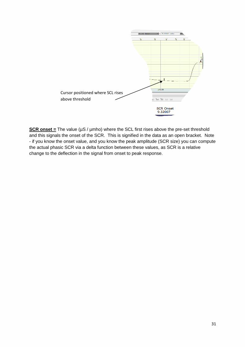
The trigger events have now been integrated into the main EDA signal and are signified in the event bar as the light-bulbs (i.e., stimulus delivery events). Once this step has been completed, the trigger channels can be hidden so that the observer can get a better look at the EDA signal. Simply hold down the Alt key while clicking on the channel number button - you can toggle the visibility of any given channel (hide or make visible).

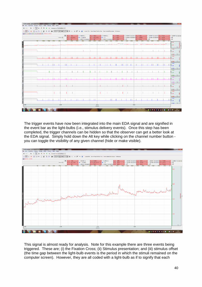
This signal is almost ready for analysis. Note for this example there are three events being triggered. These are; (i) the Fixation Cross; (ii) Stimulus presentation; and (iii) stimulus offset (the time gap between the light-bulb events is the period in which the stimuli remained on the computer screen). However, they are all coded with a light-bulb as if to signify that each

41

event is the presentation of a stimulus (which is not true). So these individual triggers need to be translated and recoded. This can be done manually (by right-clicking on the events and renaming them) - though the ideal situation is to write a script in Acqknowledge programme script to translate the stimulus trigger numbers into categorical events. This will require the additional Acqknowledge software upgrade.

A very simple approach would be; Fixation cross events = label as "Fix" and recode / label with a Flag, Stimulus presentation = label appropriately and leave as a light-bulb, Stimulus offset - recode label as "offset" and recode / label with a star. When the EDA event-related routine is then run - make sure that the stimulus event type is 'stimulus delivery' (a light bulb). This routine will now hunt for light-bulb events in the signal, it will assume these are stimulus presentations (which is now correct), and will then apply the 'preferences' and options outlined in the earlier menus to analyse as to whether or not an ER-SCR occurred.

42

Good practice for EDA measurements

Electrode contact: Good electrode contact is essential for high-quality EDA data. We recommend that sufficient time between attaching electrodes to the skin and gathering the data be provided. This is to allow for the gel to become sufficiently absorbed over the measurement area and to allow for the participant to be relaxed and ready for the experiment. Approximately 5mins would be sufficient in most cases. We also recommend some preliminary measurements be taken to assess electrode contact before the experimental measurements are taken. During this period researchers can request the participant take some sharp and deep breaths to ensure good connectivity and EDA responsiveness. Once done, if the responses are of good quality, discard these data and begin the experiment.

Ambient laboratory temperature: It is very important to maintain, as much as possible, an ambient room temperature of around 22-24-degrees Celsius. In addition, seasonal variations mean that in some cases participants may require a certain period of time in the laboratory to become accustomed to the warmer temperature in the laboratory (if it's winter) and for appropriate EDR responses to become possible. A balance between the laboratory being too hot (excessive sweating) and too cold (insufficient sweating) should be obtained with the bias being slightly on the warmer side.

Movement artefacts: Rubber-soled shoes being moved can cause sudden spikes in the EDA trace. As a consequence, all movements should be kept to a minimum. Such spikes can normally be filtered out by smoothing algorithms, however it is always desirable not to have them present in the data from the beginning. Other movement artefacts that can impact on the electrode contact points (by pulling the wires etc.) will also induce sudden artificial spikes in the trace. Stretching or pressure changes on the electrodes are other sources of error that should be avoided. It is good practice to reduce the potential for such artefacts as and when possible.

Coughs / sighs / sneezes / speech / etc: Physiological body actions like coughing, deep respiratory movements (deep sighs), sneezes and excessive talking can all generate SCRs. These are artefacts and should be avoided - especially during baseline recording periods in order to enable an artefact free measurement. Hotkeys can be set up to tag these events in the trace so that they can be accounted for in the final analysis.

Participants Approximately 10% of participants are estimated to be non-responders (hypo-responsive) in terms of their EDA. This figure can rise for studies involving some clinical groups (approx 25% and above). In addition, some participants may have cardiovascular abnormalities which can, in some circumstances, produce rhythmic artefacts (spiking) in the EDA. If all attempts to get good contacts and a good signal fail - it may well be that the participant is hypo-responsive. It may simply not be possible to obtain high quality EDA measurements from some individuals.

Section 4.0: Appendix I

43

Useful equations from the Biopac manual

Section 4.1: Appendix II