A GUIDE TO THE INTERPRETATION OF METAL CONCENTRATIONS INESTUARINE SEDIMENTS

Edited by:

Steven J. Schropp

Coastal Zone Management SectionFlorida Department of Environmental Regulation

2600 Blairstone RdTallahassee, Florida

Herbert L. Windom

Skidaway Institute of OceanographySavannah, Georgia

April 1988

-

-

EXECUTIVE SUMMARY

This document describes an approach for interpreting metalsconcentrations in coastal sediments. Interpretation ofenvironmental metals data is made difficult by the fact thatabsolute metals concentrations in coastal sediments areinfluenced by a variety of factors, including sedimentmineralogy, grain size, organic content, and anthropogenicenrichment. The interpretive tool described herein provides ameans of accounting for natural variability of metals anddetermining whether sediments are enriched with metals withrespect to expected natural concentrations.

The interpretive tool is based on the relatively constantnatural relationships that exist between metals and aluminum."Clean" coastal sediments from throughout Florida were collectedand their metals content determined. Metal/aluminum regressionsand prediction limits were calculated and diagrams ofmetal/aluminum relationships constructed. Metals data fromcoastal sediments can be plotted on these diagrams to determinewhether measured metal concentrations represent naturalconcentrations or metal enrichment.

There are several applications of this interpretive tool,including; 1) distinguishing natural versus enriched metalsconcentrations in coastal sediments, 2) comparing metalsconcentrations within an estuarine system, 3) comparing metalsconcentrations in different estuarine systems, 4) tracking theinfluence of pollution sources, 5) monitoring trends in metalsconcentrations over time, and 6) determining procedural orlaboratory errors.

The guidance in this document is intended for use byregulatory agencies, consultants, and researchers. Thegeochemical and statistical bases for the interpretive tool, useof the tool, and its limitations are described. Diagramssuitable for reproduction and use as described herein areprovided in the Appendix.

PREFACE

The work described in this document is part of broader

efforts undertaken by the Florida Coastal Management Program to

improve overall capabilities of the state for managing estuarine

resources (the "Estuarine Initiative"). This part of the

"Estuarine Initiative" suggests improvements in the way

environmental data is used in regulatory and resource management

decisions. Deficiencies in this area have played a major part in

unnecessary regulatory delays, misperception of trends, and other

-

-

-

problems in achieving balanced protection and use of coastal

resources.

In this respect, the generation and interpretation of metals

data have been of priority concern in identifying pollution

problems. The purpose of this document is to describe a method

for interpreting data on metals concentrations in estuarine

-

-sediments based on relationships that exist between metals in

natural environments.

Information presented in this document represents refinements

of previous work by the Florida Department of Environmental

Regulation, Office of Coastal Management (FDER/OCM) and

supersedes all previous FDER/OCM guidance concerning

metal/aluminum relationships.

If you have any questions or comments about the use of the

interpretive tool described in this document, please contact:

Office of Water PolicyFlorida Department of Environmental Protection3900 Commonwealth Blvd.Tallahassee, FL 32399-3000Phone: ( 8 5 0 ) - 4 8 8 - 0 7 8 4

ii

ACKNOWLEDGEMENTS

-

This work was supported by a grant from the Office of Ocean

and Coastal Resource Management, National Oceanic and Atmospheric

Administration, through the Coastal Zone Management Act of 1972,

as amended. The efforts of Graham Lewis, Joe Ryan, Lou Burney,

and Fred Calder in developing and conducting the sampling program

and in reviewing this document were an integral part of this

project. Appreciation is extended to Duane Meeter and Kevin

Carman for their advice and assistance on statistical aspects of

the work.

iii

TABLE OF CONTENTS

EXECUTIVE SUMMARY

PREFACE . . . .

ACKNOWLEDGEMENTS .

LIST OF TABLES .

LIST OF FIGURES .

. .

. ..

. .

. .

. .

. .

. .

. .

. .

. .

. .

. .

. .

. .

. .

. .

. .

. .

. .

. .

. .

. .

. .

. .

. .

. .

. .

. .

. .

. .

MANAGEMENT ISSUES AND TECHNICAL BACKGROUND

GEOCHEMICAL BASIS FOR AN INTERPRETIVE TOOLA REFERENCE ELEMENT . . . . . . . . .

. . .

. . .

. . .

. . .

. . .

. . .

. .

. .

. .

. .

. .

. .

. .

. .

. .

. .

. .

. .

. .

. .

. .

. .

. .

. .

USING ALUMINUM AS. . . . . . .

DEVELOPMENT OF AN INTERPRETIVE TOOL USING METAL/ALUMINUMRELATIONSHIPS . . . . . . . . . . .

USING THE INTERPRETIVE TOOL . . . . . .

APPLICATIONS OF THE INTERPRETIVE TOOL .

LIMITATIONS OF THE INTERPRETIVE TOOL .

EXAMPLES . . . . . . . . . . . . . . .

REFERENCES . . . . . . . . . . . . . .

APPENDIX . . . . . . . . . . . . . . .

. .

. .

. .

. .

. .

. .

. .

. .

. .

. .

. .

. .

. .

. .

. .

. .

. .

. .

. .

. .

. .

. .

. .

. .

. .

. .

. .

. .

. .

. l

. .

. .

. .

. .

. .

. .

i

ii

iii

V

v i

1

4

12

30

31

33

36

43

A-l

i v

TABLES

TABLE 1. Relative abundance of metals in Crustalmaterials.......................................7

TABLE 2. Results of probability plot correlationcoefficient tests for normality of metals data . 17

TABLE 3. Correlation coefficients for metals and aluminum . 19

TABLE 4. Results of probability plot correlationcoefficient tests for normality of metal/aluminum ratios.........................20

TABLE 5. Results of regression analyses using aluminumas the independent variable and other metals asdependent variables..............................29

V

FIGURES

FIGURE

FIGURE

FIGURE

FIGURE

FIGURE

FIGURE

FIGURE

FIGURE

FIGURE

FIGURE

FIGURE

1. Schematic representation of the weatheringp r o c e s s . . . . . . . . . . . . . . . . . . . . . . .

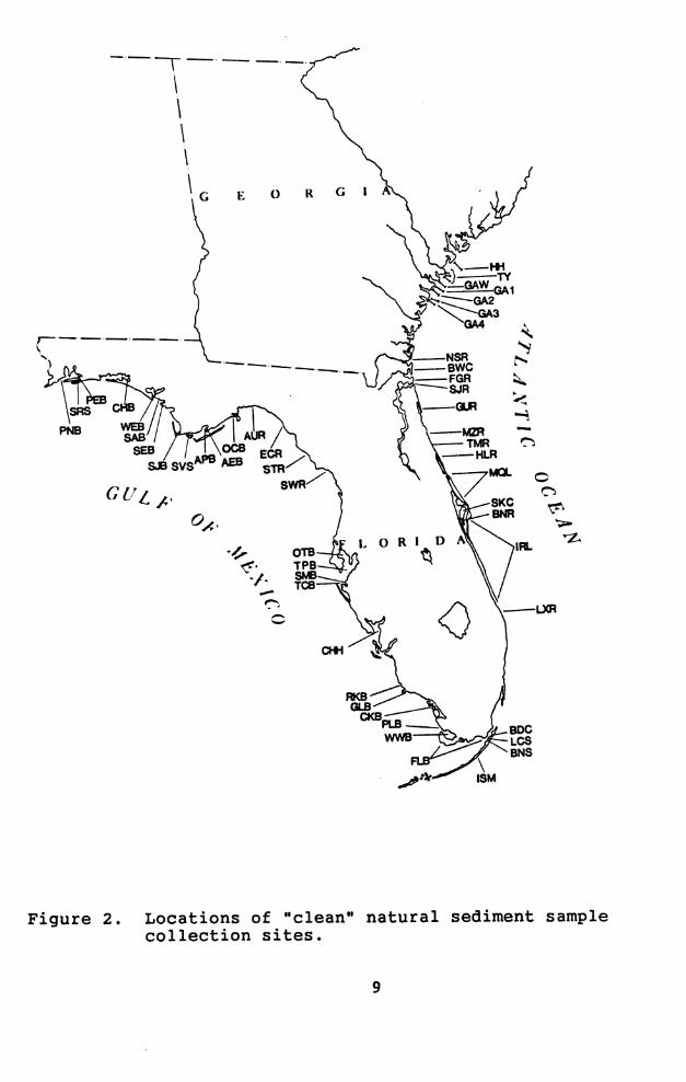
2. Locations of "clean" natural sediment samplecollection sites.........................

3. Metal/aluminum relationships in sediments off theGeorgia.coast.........................

4. Metal/aluminum relationships in "clean" sedimentsfrom Florida estuaries..................

5. Mean value vs. standard deviation for chromium:(a) untransformed data, b) log-transformed data...

6. Normal score vs. chromium value:(a) untransformed data, b) log-transformed data...

7. Metal/aluminum relationships for log-transformedmetals in "clean" Florida estuarine sediments....

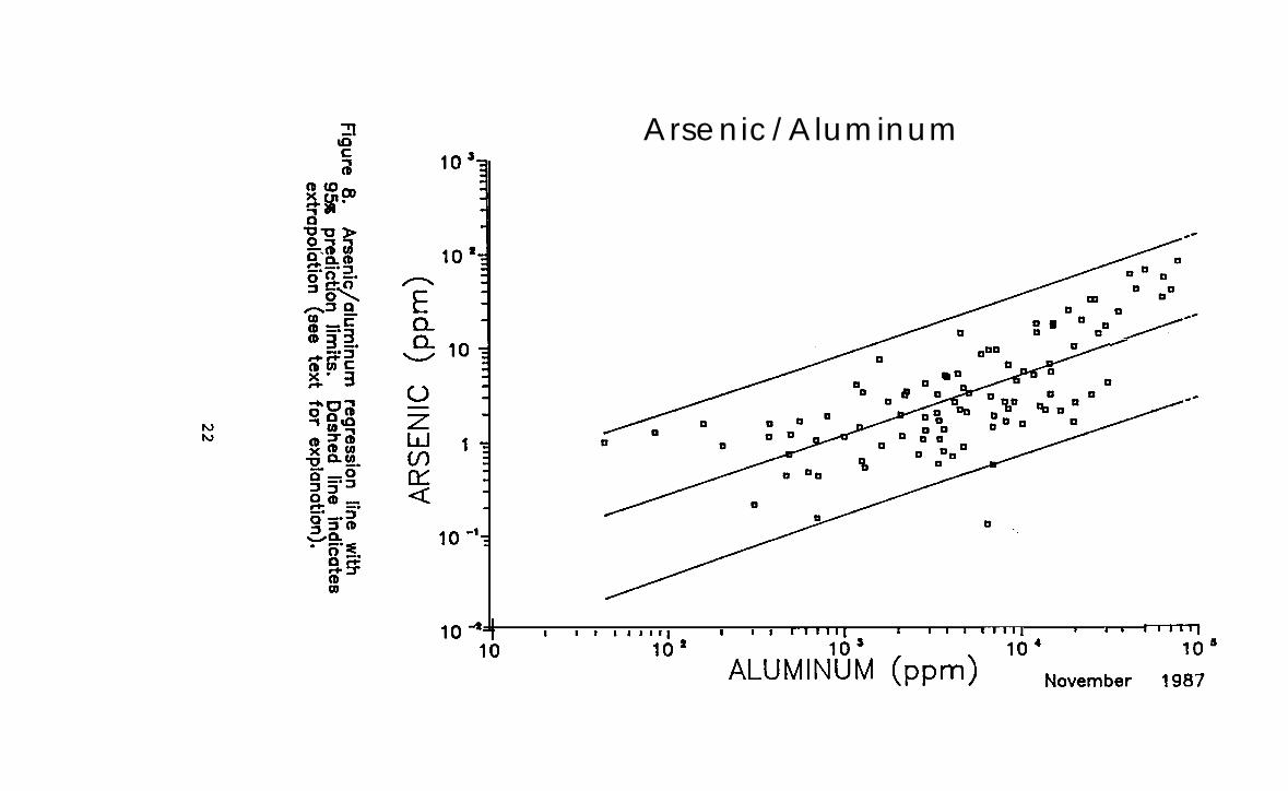
8. Arsenic/aluminum regression line with95% prediction limits . . . . . . . . . . . . . . .

9. Cadmium/aluminum regression line with95% prediction limits . . . . . . . . . . . . . . .

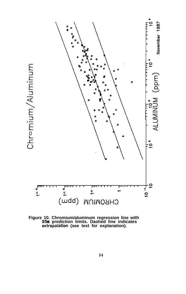
10. Chromium/aluminum regression line with95% prediction limits...................

5

9

10

13

15

16

18

22

23

24

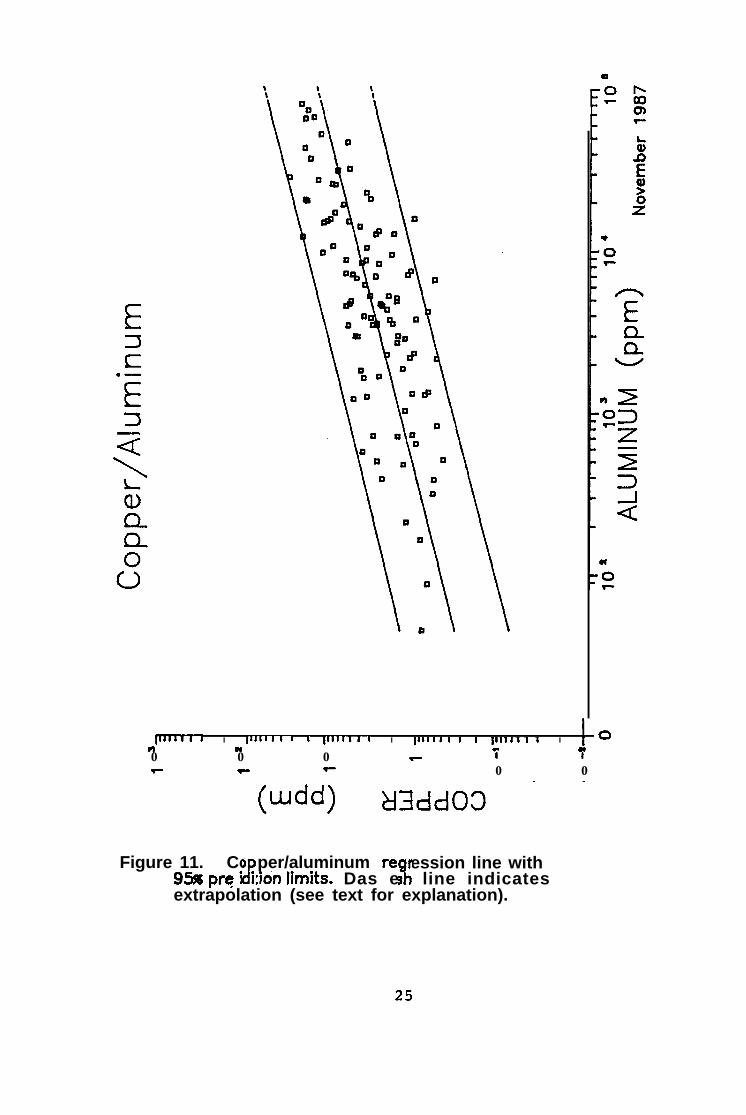
11. Copper/aluminum regression line with95% prediction limits...................25

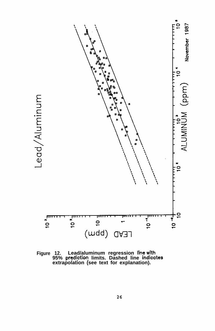
FIGURE 12. Lead/aluminum regression line with95% prediction limits...................26

FIGURE 13. Nickel/aluminum regression line with95% prediction limits...................27

FIGURE 14. Zinc/aluminum regression line with95% prediction limits...................28

FIGURE 15. Hypothetical estuary showing sampling stationsand sediment grain size .......................37

FIGURE 16. Chromium results from hypothetical estuarinesampling stations shown in Figure 15...............39

FIGURE 17. Hypothetical estuary showing metal source,sampling stations, and sediment grain size.....41

FIGURE 18. Chromium results from hypothetical estuarinesampling stations shown in Figure 17.......42

vi

Florida has an extensive coastline (approximately 11,000

MANAGEMENT ISSUES AND TECHNICAL BACKGROUND

_.miles) and an unusual diversity of estuarine types. Conditions

in its many estuaries range from nearly pristine to localized

severe degradation. Metals are of particular concern in terms of

protecting and rehabilitating estuaries, not only because of

their potential toxic effects, but also because high metals

concentrations can be a signal for the presence of other types of

pollution.

Estuarine management efforts generally suffer from several

types of deficiencies in terms of understanding and dealing with

metals

1.

2.

3.

4.

pollution. Among these are the following:

Difficulty in comparing estuarine systems and

establishing priorities for management actions.

Difficulty in distinguishing actual or potential problems

from perceived problems.

Unnecessary delays in permitting, attributable to

improper generation and interpretation of metals data.

Difficulty in establishing cost-effective means for

assessing pollution trends and frameworks for

understanding overall estuarine pollution.

The problem of understanding metals pollution has at least

two major aspects. One aspect involves distinguishing those

components attributable to natural causes from those attributable

to man's activities. The second aspect involves determining

whether metals in anthropogenically enriched sediments are

potentially available for recycling to the water column or

1

through food chains in amounts likely to adversely affect water

quality and living resources. Guidance in this document deals

with the first aspect: the determination of natural versus

unnatural concentrations of metals. In doing so, it sets the

stage for addressing the second aspect: effects of enriched metal

concentrations.

In order to address both of these aspects, it is necessary to

have at least a general understanding of the geochemical

processes that govern the behavior and fate of metals in

estuaries and marine waters. Natural metal concentrations can

vary widely among estuaries. In Florida, which has a wide range

of estuarine types, this presents special difficulties for making

statewide comparisons of estuarine systems and for making

consistent, scientifically defensible regulatory decisions. The

interpretive approach discussed in this document was developed to

account for natural variability in metals concentrations and to

help identify anthropogenic inputs.

The tool for interpreting metal concentrations in estuarine

sediments is based on demonstrated, naturally occurring

relationships between metals and aluminum. Specifically, natural

metal/ aluminum relationships were used to develop guidelines for

distinguishing natural sediments from contaminated sediments for

a number of metals and metalloids commonly released to the

environment due to anthropogenic activities. Aluminum was chosen

as a reference element to normalize sediment metals

concentrations for several reasons: it is the most abundant

-

-

-

-

-

-

-

-

2

-

_

naturally occurring metal; it is highly refractory; and its

concentration is generally not influenced by anthropogenic

sources.

To ensure that the information used to develop the

interpretive tool was representative of the diverse Florida

sediments, uncontaminated sediments from around the state were

examined for their metal content and the natural variability of

metal/aluminum relationships was statistically assessed.

This approach to the interpretation of metals data was

initially described in two documents prepared by FDER/OCM: 1)

"Geochemical and Statistical Approach for Assessing Metals

Pollution in Estuarine Sediments" (FDER/OCM, 1986a) and 2) "Guide

to the Interpretation of Reported Metal Concentrations in

Estuarine Sediments" (FDER/OCM, 1986b). Information presented in

this document represents further refinements of the approach,

using an improved and expanded data base and a more rigorous

statistical treatment of metal/aluminum relationships. This

document supersedes all previous guidance by FDER/OCM concerning

metal/aluminum relationships.

-

-

3

GEOCHEMICAL BASIS FOR AN INTERPRETIVE TOOL USING ALUMINUM AS A

REFERENCE ELEMENT

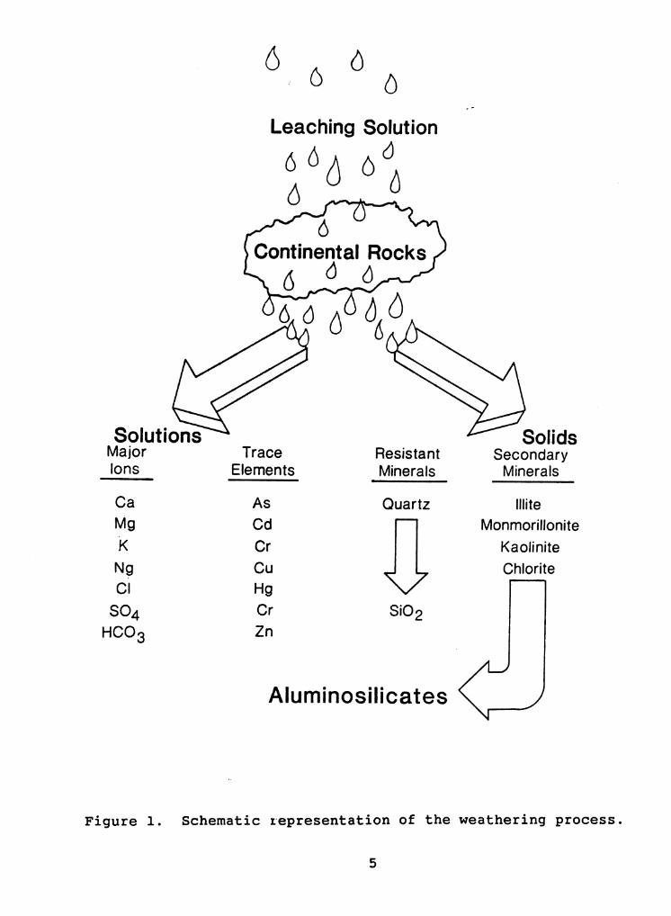
Natural estuarine sediments are predominantly composed of

river-transported debris resulting from continental weathering.

A schematic representation of the weathering process is given in

Figure 1. Acids formed in the atmosphere or from the breakdown

of organic matter (e.g., carbonic, humic fulvic acids) mix with

water and form leaching solutions. These leaching solutions

break down rocks and carry away the products in solution or as

solid debris. The solid debris is composed chiefly of

chemically resistant minerals, such as quartz and secondary clay

minerals, which are the alteration products of other

aluminosilicate minerals. The aluminosilicate clay minerals are

represented by the general formula MOAlSi04, where M = naturally

occurring metal that can substitute for aluminum in the

aluminosilicate structure, Al = aluminum, Si = silicon, and 0 =

oxygen. The metals are tightly bound within the aluminosilicate

lattice.

The weathering solution also contains dissolved metals that

have been leached from the parent rock. Because of their low

solubilities, however, metals are present in the transporting

solution (e.g., rivers) in very low amounts, on the order of

nanomolar (10-g liter-l) concentrations. Thus, most of

metals transported by rivers are tightly bound in the

aluminosilicate solid phases. As a consequence, during

the

weathering, there is very little fractionation between the

naturally occurring metals and aluminum.

4

_-

-

-

-

-

-

-

-

-

-

Leaching Solution

-MajorIons

-

-

Ca

MgK

NgCL

- SO4HC03

TraceElements

AsCdCrcu

HgHgCrZn

Quartz

SiO2

IIIiteMonmorillonite

KaoliniteChlorite

Aluminosilicates

Resistant SecondaryMinerals Minerals

Figure 1. Schematic representation of the weathering process.

5

-

In general, when dissolved metals from natural or

anthropogenic sources come in contact with saline water they

quickly adsorb to particulate matter and are removed from the

water column to bottom sediments. Thus, metals from both natural -

and anthropogenic sources are ultimately concentrated in

estuarine sediments, not the water column.

Since much of the natural component of metals in estuarine -

sediments is chemically bound in the aluminosilicate structure,

the metals are generally non-labile. The adsorbed anthropogenic -

or "pollutant" component is more loosely bound. Metals in the-

anthropogenic fraction, therefore, may be more available to

estuarine biota and may be released to the water column in -

altered forms when sediments are disturbed (e.g., by dredging or

storms). -

Aluminum is the second most abundant metal in the earth's-

crust (silicon being the most abundant). Results from several

studies have indicated that the relative proportions of metals -

and aluminum in crustal material are fairly constant (Martin and

Whitfield, 1983; Taylor, 1964; Taylor and McLennan, 1981; -

Turekian and Wedepohl, 1961). This is not surprising given the

-lack of large-scale fractionation of metals and aluminum during

weathering processes. The average metal concentration of various-

materials that make up the earth's crust are given in Table 1.

6

-

-

-

-

-

-

-

-

-

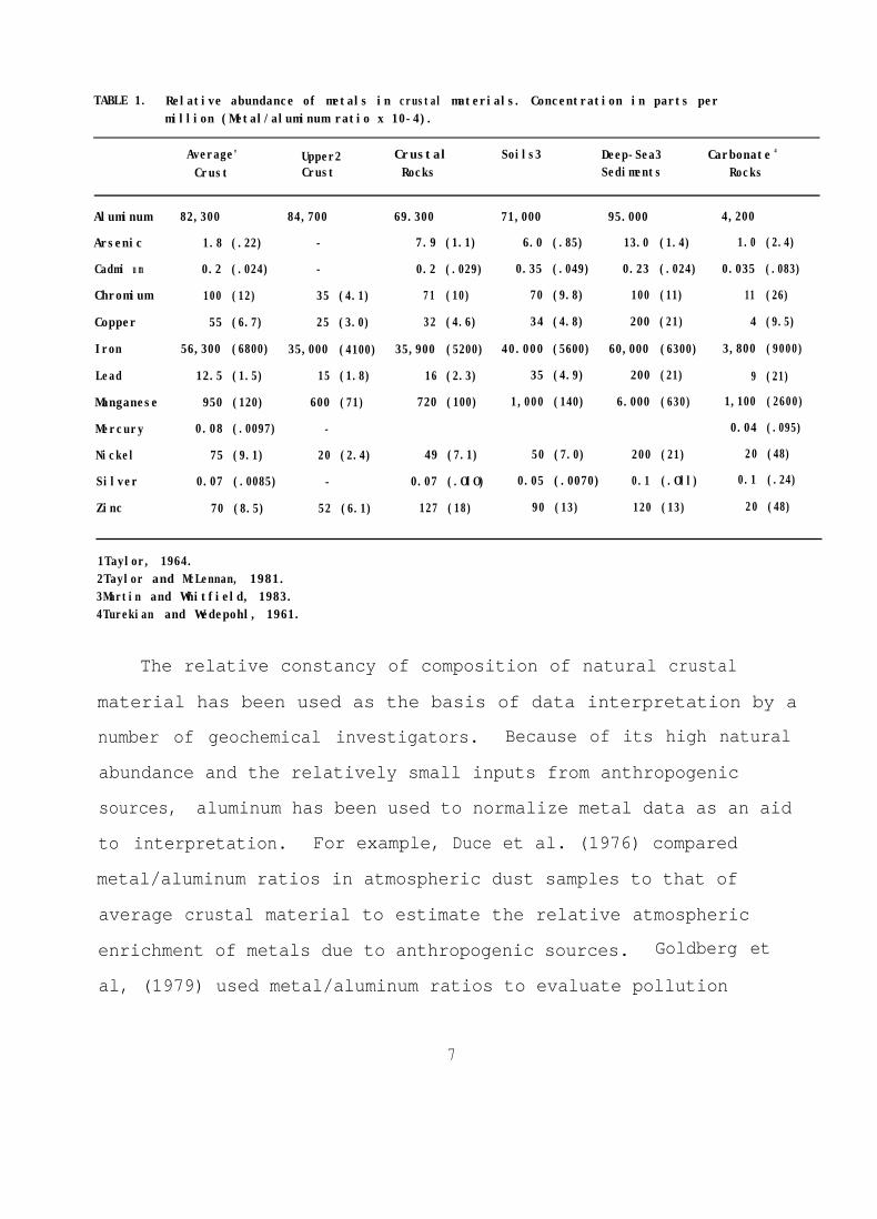
TABLE 1. Relative abundance of metals in crustal materials. Concentration in parts permillion (Metal/aluminum ratio x 10-4).

Average'Crust

Upper2Crust

CrustalRocks

Soils3 Deep-Sea3Sediments

Carbonate 4

Rocks

Aluminum

Arsenic

Cadmi u m

Chromium

Copper

Iron

Lead

Manganese

Mercury

Nickel

Silver

Zinc

82,300 84,700

1.8 (.22) -

0.2 (.024) -

100 (12) 35 (4.1)

55 (6.7) 25 (3.0)

56,300 (6800) 35,000 (4100)

12.5 (1.5) 15 (1.8)

950 (120) 600 (71)

0.08 (.0097) -

75 (9.1) 20 (2.4)

0.07 (.0085) -

70 (8.5) 52 (6.1)

69.300 71,000 95.000

7.9 (1.1) 6.0 (.85) 13.0 (1.4)

0.2 (.029) 0.35 (.049) 0.23 (.024)

71 (10) 70 (9.8) 100 (11)

32 (4.6) 34 (4.8) 200 (21)

35,900 (5200) 40.000 (5600) 60,000 (6300)

16 (2.3) 35 (4.9) 200 (21)

720 (100) 1,000 (140) 6.000 (630)

49 (7.1)

0.07 (.OlO)

127 (18)

50 (7.0) 200 (21)

0.05 (.0070) 0.1 (.Oll)

90 (13) 120 (13)

4,200

1.0 (2.4)

0.035 (.083)

11 (26)

4 (9.5)

3,800 (9000)

9 (21)

1,100 (2600)

0.04 (.095)

20 (48)

0.1 (.24)

20 (48)

1Taylor, 1964.2Taylor and McLennan, 1981.3Martin and Whitfield, 1983.4Turekian and Wedepohl, 1961.

The relative constancy of composition of natural crustal

material has been used as the basis of data interpretation by a

number of geochemical investigators. Because of its high natural

abundance and the relatively small inputs from anthropogenic

sources, aluminum has been used to normalize metal data as an aid

to interpretation. For example, Duce et al. (1976) compared

metal/aluminum ratios in atmospheric dust samples to that of

average crustal material to estimate the relative atmospheric

enrichment of metals due to anthropogenic sources. Goldberg et

al, (1979) used metal/aluminum ratios to evaluate pollution-

7

history recorded in sediments from the Savannah River estuary.

Trefry et al. (1985) compared lead levels to those of aluminum in

sediments of the Mississippi delta to assess the changes in

relative amounts of lead pollution carried by the river over the

past half century.

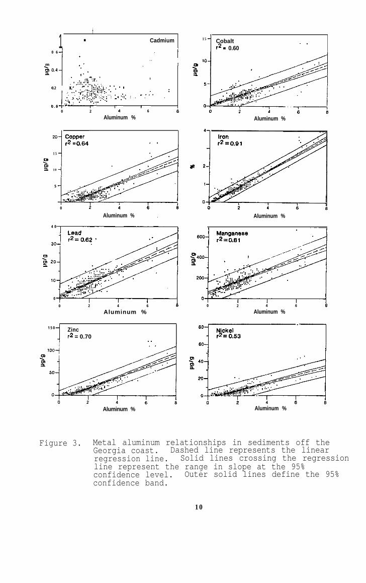
If a metal such as aluminum is to be useful to normalize

metal concentrations for the purpose of distinguishing natural

versus unnatural metal levels in sediments, it must explain most

of the natural variance in the concentrations of the other

metals. This assumption has been tested for natural sediments

along the coast of Georgia (Figure 2, stations along transects

HH - GA4). The results of the analysis of over three hundred

sediment samples are presented in Figure 3. Metal concentrations

are plotted against aluminum; regression lines and confidence

limits are also plotted. These results indicate that for this

geographic area aluminum does account for most of the variability

of the other metals except cadmium. For cadmium, the low natural

concentrations are such that analytical uncertainty introduces

another source of variance.

The above shows that using aluminum to normalize natural

metal concentrations is an approach that works, at least for a

relatively localized area. But will this approach work for more

diverse sediments such as those of coastal Florida?

Estuarine and coastal sediments of Florida contain natural

metal-bearing phases. In south Florida, however, many sediments

are carbonate-rich. Inspection of Table 1, indicates that

-

-

-

-

-

-

-

-

-

-

-

8

-

1 . * Cadmium

0 6

. .m I

*. *. :!L .I’.. * ,::!.“,*., . . .

0.2 I.’ ** * !I;~*!.:~~. - *. - I

I’ /* s: :

. ..’ .i”“::“!’ i:.!‘:. ‘.. . .I. “1. . . .

. ..* .*: ;;!:.::jI .:::*: : ** 1.:: : . * . * **.*

.

* : : .I..... *0 . 0 ‘i-

0 2 4 6 6

Aluminum %

. .

15 1 Cobaltr2 = 0.60

. .-

lo-

Pz!

Aluminum %

15

m23a 10

5 1

0

0 iAluminum % .

4 0

0

0 2 4 6 a

Aluminum %

i i iAluminum %

0 2 4 6 8

Aluminum %

1 5 0

I

Zincr2 = 0.70 . .

Aluminum % Aluminum %

-

-

-

-

-

-

-

Figure 3. Metal aluminum relationships in sediments off theGeorgia coast. Dashed line represents the linearregression line. Solid lines crossing the regression -line represent the range in slope at the 95%confidence level. Outer solid lines define the 95%confidence band.

10

-

1 . * Cadmium

0 6

. .m I

*. *. :!L .I’.. * ,::!.“,*., . . .

0.2 I.’ ** * !I;~*!.:~~. - *. - I

I’ /* s: :

. ..’ .i”“::“!’ i:.!‘:. ‘.. . .I. “1. . . .

. ..* .*: ;;!:.::jI .:::*: : ** 1.:: : . * . * **.*

.

* : : .I..... *0 . 0 ‘i-

0 2 4 6 6

Aluminum %

. .

15 1 Cobaltr2 = 0.60

. .-

lo-

Pz!

Aluminum %

15

m23a 10

5 1

0

0 iAluminum % .

4 0

0

0 2 4 6 a

Aluminum %

i i iAluminum %

0 2 4 6 8

Aluminum %

1 5 0

I

Zincr2 = 0.70 . .

Aluminum % Aluminum %

-

-

-

-

-

-

-

Figure 3. Metal aluminum relationships in sediments off theGeorgia coast. Dashed line represents the linearregression line. Solid lines crossing the regression -line represent the range in slope at the 95%confidence level. Outer solid lines define the 95%confidence band.

10

-

-

-

-

-

-

-

-

-

-

-

carbonate sediments have larger metal/aluminum ratios than other

crustal rocks. Table 1 also suggests, however, that carbonates

contain relatively smaller concentrations of most metals as

compared to typical crustal material. It follows, therefore,

that in a sediment containing a mix of aluminosilicates and

carbonates, aluminosilicate minerals would still be the most

important metal-bearing phase and that aluminum could still be

used to normalize metal concentrations. Thus, aluminum

concentrations should also be appropriate for normalizing metal

levels in most estuarine and coastal sediments of Florida.

To test whether aluminum can be used to normalize metal

concentrations in Florida coastal sediments, sediment samples

from 103 stations in uncontaminated estuarine/coastal areas were

collected and analyzed for aluminum and a number of

environmentally and geochemically important metals. The areas

involved encompassed a variety of sediment types ranging from

terrigenous, aluminosilicate-rich sediments in northern Florida

to biogenic, carbonate-rich sediments in southern Florida (Figure

2). These "clean" sites were selected subjectively, based upon

their remoteness from known or suspected anthropogenic metal

sources.

At each station, to ensure retrieval of undisturbed sediment

samples, divers collected sediments in cellulose-acetate-butyrate

cores. Sediment for metals analyses was taken from the upper

five centimeters of each core. Duplicate samples were taken at

each station and analyzed for nine metals (aluminum, arsenic,

cadmium, chromium, copper, mercury, nickel, lead, zinc) according-

11

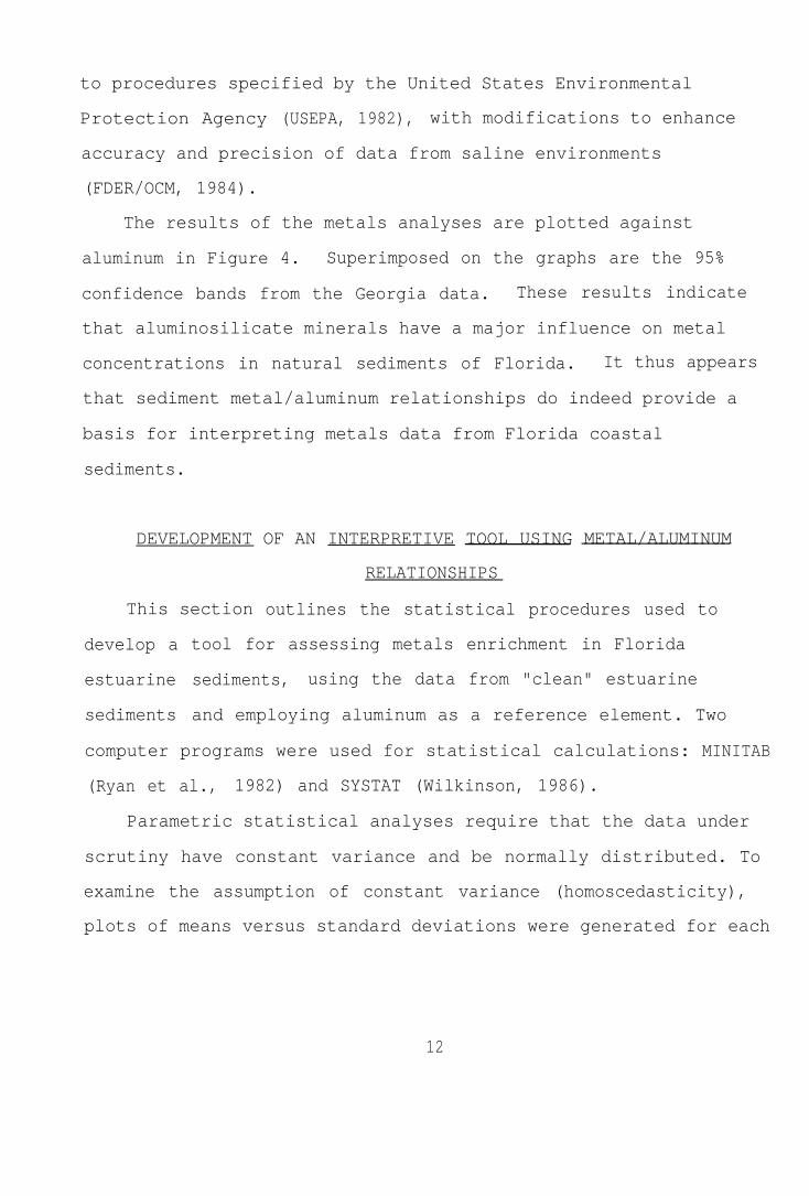
to procedures specified by the United States Environmental

Protection Agency (USEPA, 1982),, with modifications to enhance

accuracy and precision of data from saline environments

(FDER/OCM, 1984).

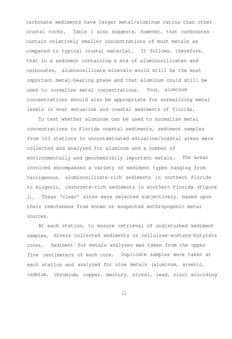
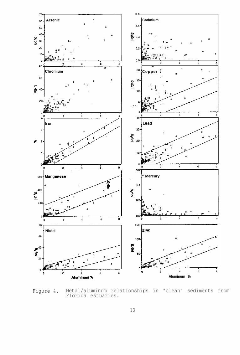
The results of the metals analyses are plotted against

aluminum in Figure 4. Superimposed on the graphs are the 95%

confidence bands from the Georgia data. These results indicate -

that aluminosilicate minerals have a major influence on metal

concentrations in natural sediments of Florida. It thus appears-

that sediment metal/aluminum relationships do indeed provide a-

basis for interpreting metals data from Florida coastal

sediments.

DEVELOPMENT OF AN INTERPRETIVE TOOL USING METAL/ALUMINUM -

RELATIONSHIPS

This section outlines the statistical procedures used to

-

-

develop a

estuarine

sediments

tool for assessing metals enrichment in Florida -

sediments, using the data from "clean" estuarine

and employing aluminum as a reference element. Two -

computer programs were used for statistical calculations: MINITAB-

(Ryan et al., 1982) and SYSTAT (Wilkinson, 1986).

Parametric statistical analyses require that the data under -

scrutiny have constant variance and be normally distributed. To

examine the assumption of constant variance (homoscedasticity), -

plots of means versus standard deviations were generated for each-

12

?O-

6o _ Arsenic I Cadmium

0.6

-

- n 4 6 0 2 4 6

1”

2o Copper t0 0 0oChromium

60

00 2 4 6 8

402 4 6 a

600

40099

200

0

-

0n 2 4 6 a

_O Mercury

0.4-0

0

-

0.00 2 4 6 a-

0 2 4 6 6

150

Nickel

60100

P9

50

00 2 4 6 a

$09

20

00 2 4 6 6

Aluminum 96 Aluminum %

Figure 4. Metal/aluminum relationships in "clean" sediments fromFlorida estuaries.

13

metal. Standard deviations were proportional to mean values for

all nine metals. After a log10 transformation, the

proportionality between standard deviations and mean values was

removed, indicating that the assumption of homoscedasticity was

satisfied. Examples of these plots before and after

transformation, using the data for chromium, are shown in

Figure 5.

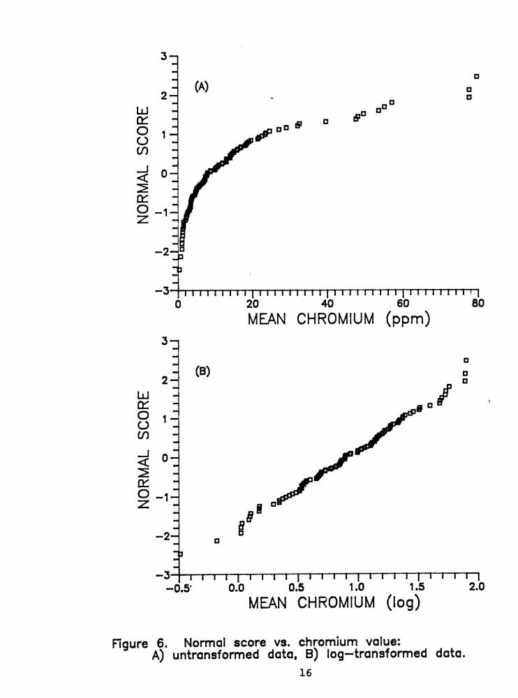
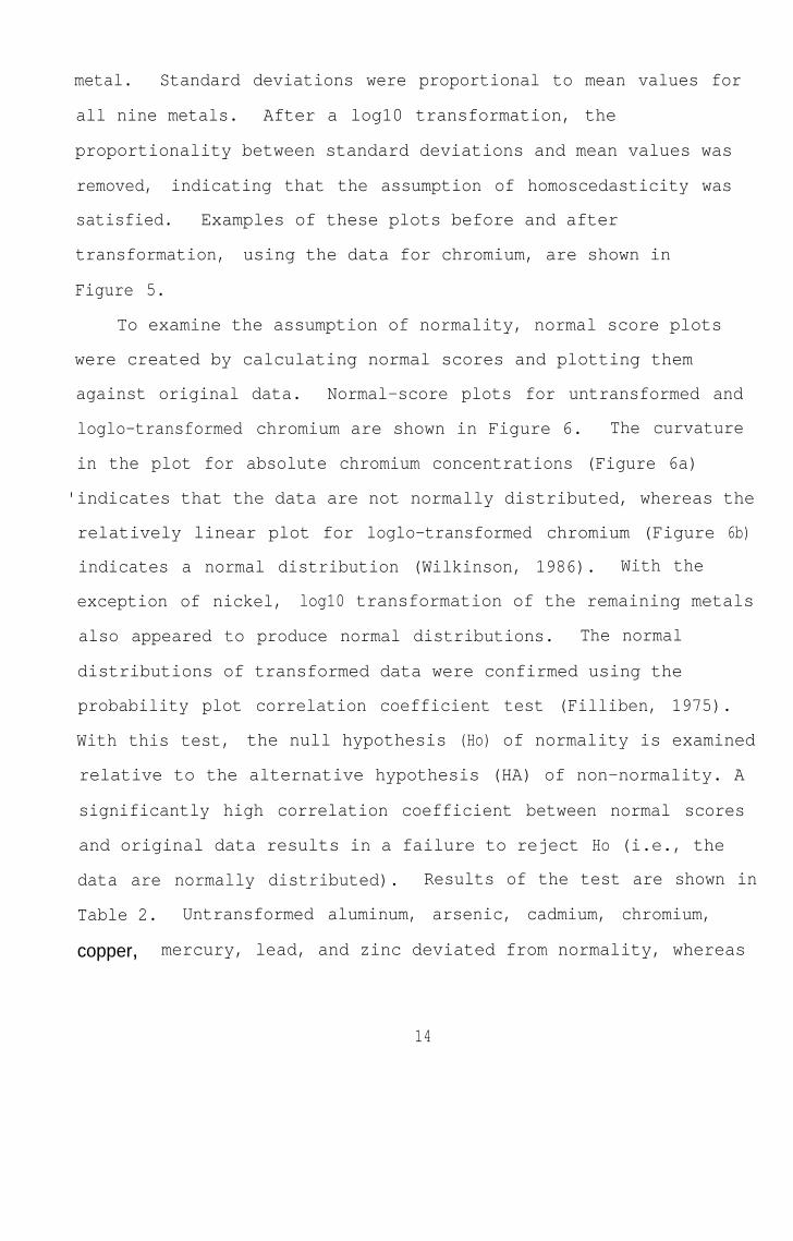
To examine the assumption of normality, normal score plots

were created by calculating normal scores and plotting them

-

-

-

against original data. Normal-score plots for untransformed and-

loglo-transformed chromium are shown in Figure 6. The curvature

in the plot for absolute chromium concentrations (Figure 6a) -

'indicates that the data are not normally distributed, whereas the

relatively linear plot for loglo-transformed chromium (Figure 6b) -

indicates a normal distribution (Wilkinson, 1986). With the

-exception of nickel, log10 transformation of the remaining metals

also appeared to produce normal distributions. The normal -

distributions of transformed data were confirmed using the

probability plot correlation coefficient test (Filliben, 1975). -

With this test, the null hypothesis (Ho) of normality is examined

-relative to the alternative hypothesis (HA) of non-normality. A

significantly high correlation coefficient between normal scores -

and original data results in a failure to reject Ho (i.e., the

data are normally distributed). Results of the test are shown in _

Table 2. Untransformed aluminum, arsenic, cadmium, chromium,

copper, mercury, lead, and zinc deviated from normality, whereas-

-

-14

25

3

-

-

-

-

-

-

095 20

i=Q

zi 15f3 0

a0

00 00 0

MEAN CHROMIUM (ppm)

0.5

g 0.4

5-

z 0.3n i

0.0 j~~II~llllJlJl~~~~~~~~~~~i-0.3 0.0

MEAN”‘;HROM;;JoM (lo;;2.0

@I 0

Figure 5. Mean value vs. standard deviation for chromium:A) untransformed data, B) log-transformed data.

15

-3~,,,,,,,,,,,,,,,,,,,,,,,,,,,,,,,,,~~~~~I~20 40 60 '806

39

2-

ifi!

8 '-VI

2 O'Izz

zL.Iz '-

-2-

MEAN CHROMIUM (ppm)

MEAN CHROMIUM (log)

Figure 6. Normal score vs. chromium value:A) untransformed data, B) log-transformed data.

16

-

-

-

-

.-

-

-

-

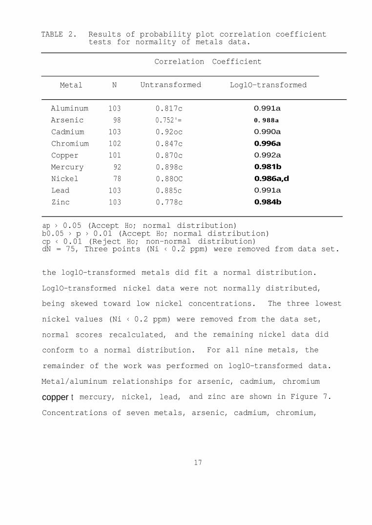
TABLE 2. Results of probability plot correlation coefficienttests for normality of metals data.

Correlation Coefficient

Metal N Untransformed LoglO-transformed

Aluminum 103

Arsenic 98

Cadmium 103

Chromium 102

Copper 101

Mercury 92

Nickel 78

Lead 103

Zinc 103

0.817c

0.752'=

0.92oc

0.847c

0.870c

0.898c

0.88OC

0.885c

0.778c

0.991a

0.988a

0.990a

0.996a

0.992a

0.981b

0.986a,d

0.991a

0.984b

ap > 0.05 (Accept Ho; normal distribution)b0.05 > p > 0.01 (Accept Ho; normal distribution)cp < 0.01 (Reject Ho;dN

non-normal distribution)= 75, Three points (Ni < 0.2 ppm) were removed from data set.

the loglO-transformed metals did fit a normal distribution.

LoglO-transformed nickel data were not normally distributed,

being skewed toward low nickel concentrations. The three lowest

nickel values (Ni < 0.2 ppm) were removed from the data set,

normal scores recalculated, and the remaining nickel data did

conform to a normal distribution. For all nine metals, the

remainder of the work was performed on loglO-transformed data.

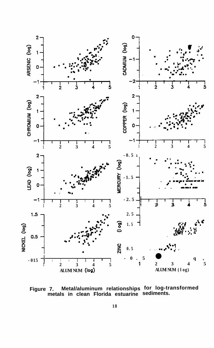
Metal/aluminum relationships for arsenic, cadmium, chromium

copper t mercury, nickel, lead, and zinc are shown in Figure 7.

Concentrations of seven metals, arsenic, cadmium, chromium,

17

. .

I I I I I I I I1 2 3 4 5

..

.l . -0

-1 I I I I I I I I1 2 3 4 5

.

-015 1 I I I I I 1 ’ I1 2 3 4 5

ALUMINUM (log)

Ol

.

..

.

0.

. + . l ,;-’l . I’

. I l .. 0..

. n==.q :l y@

mm_= ,=;.da .I% .l . .

. . .I I’. .

.l . ‘

-‘l1 2 3 4 5

-0.5 1

G

i

’ . l .. 0

.9

. ..=. 0.. l

. ==

i

-0 ;cr: 0 . l =

. '.. .8

-1.5 + .

Ei

. ;mlp.,I).y"". . . _Y.mm

I

-2.5 .I'I';1 2 3 4

2.5 1

‘C3 1.5 c’ 0

a.

; 0.5

1. . .

.&$f :.: SC

a. .id .A.,

- 0 . 5 l q ,2 3 4 5iALUMINUM (log)

Figure 7. Metal/aluminum relationships for log-transformedmetals in clean Florida estuarine sediments.

18

-

-

-

-

-

-

-

-

-

-

-

-

-

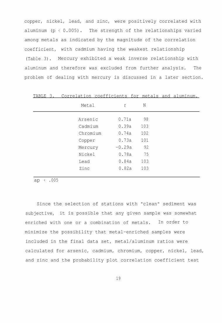
copper, nickel, lead, and zinc, were positively correlated with

aluminum (p < 0.005). The strength of the relationships varied

among metals as indicated by the magnitude of the correlation

coefficient, with cadmium having the weakest relationship

(Table 3). Mercury exhibited a weak inverse relationship with

aluminum and therefore was excluded from further analysis. The

problem of dealing with mercury is discussed in a later section.

TABLE 3. Correlation coefficients for metals and aluminum.

Metal r N

-

ap < .005

-

-

-

Arsenic

Cadmium

Chromium

Copper

Mercury

Nickel

Lead

Zinc

0.71a 98

0.39a 103

0.74a 102

0.73a 101

-0.29a 92

0.78a 75

0.84a 103

0.82a 103

Since the selection of stations with "clean" sediment was

subjective, it is possible that any given sample was somewhat

enriched with one or a combination of metals. In order to

minimize the possibility that metal-enriched samples were

included in the final data set, metal/aluminum ratios were

calculated for arsenic, cadmium, chromium, copper, nickel, lead,

and zinc and the probability plot correlation coefficient test

19

was used to determine whether the ratios were normally

distributed. If the correlation coefficient test indicated

deviations from normality, data points with the largest

metal/aluminum ratio were removed (assuming that high ratios were

possibly indicative of anthropogenic enrichment) and the process

repeated until the metal/aluminum ratios fit a normal

distribution. Results are shown in Table 4. Data points for -

three metals (cadmium, zinc, lead) were deleted from the data set

using this procedure. -

TABLE 4. Results of probability plot correlation coefficienttests for normality of metal/aluminum ratios.

"Clean" "Trimmed-clean"data data

Ratio N r N r

Arsenic/aluminum 98 0.988a 98 0.988a

Cadmium/aluminum 103 0.96gc 102 0.983b

Chromium/aluminum 102 0.988a 102 0.988a

Copper/aluminum 101 0.988a 101 0.988a

Nickel/aluminum 75 0.911c 72 0.987a

Lead/aluminum 103 0.955c 93 0.993a

Zinc/aluminum 103 0.934c 99 0.985b

ap > 0.05 (Accept Ho; normal distribution).b0.05 > p > 0.01 (Accept Ho; normal distribution).cp < 0.01 (Reject Ho; normal distribution).

Nickel again presented a different case, with the

distribution of nickel/aluminum ratios being skewed toward low

-

-

-

-

-

-

-

-

ratios. After removal of three points with the lowest-

20-

-

-

-

-

-

-

-

-

-

-

nickel/aluminum ratios, the remaining nickel/aluminum ratios fit

a normal distribution. The metals data set resulting from the

deletion of points was called the "trimmed clean" data set and

was used for subsequent analyses.

Having ascertained that the data does meet the assumptions of

normality and homoscedasticity, and having examined metal/

aluminum ratios for outlying data points, the data were then

analyzed using parametric statistical procedures. Least squares

regression analysis, using aluminum as the independent variable

and other metals as dependent variables, was used to fit

regression lines to the metals of the "trimmed clean" data set

(Sokal and Rohlf, 1969). Results of the regressions are

presented in Table 5. Correlation coefficients for three of the

"trimmed" metals (cadmium, lead, zinc) were greater than those

for the original data, indicating the relationship between these

metals and aluminum in the "trimmed clean" data set was

strengthened by removing the suspect points. Y-intercepts of the

regression lines are less than zero because the data were loglo-

transformed.

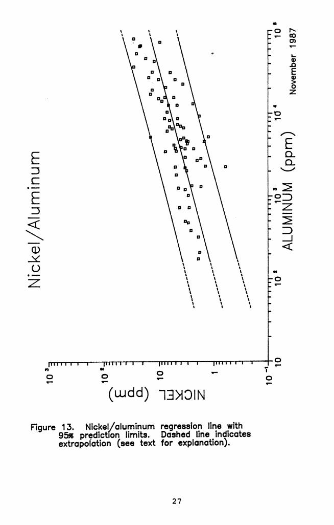
Using the regression results, 95% prediction limits were

calculated according to Sokal and Rohlf (1969). Regression lines

and prediction limits for each metal are plotted in Figures 8-14,

superimposed over data points from the "trimmed clean" data

set. The relative width of the prediction limits vary among the

different metals, depending on the magnitude of the correlation

between the metal and aluminum. Metals with the largest

correlation coefficients (i.e., lead & zinc) have the narrowest

prediction limits.

21

Arsenic/Aluminum

1 I I IIIII~ I I I IllIll 1 I I I IIIII I I I IllIll

10 10' ALuMd& (ppm) lo4 November 19t’

I I I I I I I

I I

h)W

I I I I I I I

Cadmium/Aluminum

- 1 "Enn

22 -1,___---

3’O !f

a

2 __-- e-0 00 ma 0 0

u

10 -=<

lo4 1 I I lllll~ I I I I IIIII I I I lllll~ I I I IllIll

1 0 lo2AL~fd8ii (ppm) lo4 November 19gs

E

3.-

E0

k(I

- 36

w

r’oF

I”” ’ ’ ’ ’ I”“’ ’ ’ ’ I”” ’ ’ ’ ’ I”“’ ’ ’ ’ 0n u

0 v 7F

0 0 rF C

0T-

(udd) b'VlIl'lOklH3

Figure 10. Chromium/aluminum regression line with95% prediction limits. Dashed line indicatesextrapolbtion (see text for explanation).

-

-

-

24

-

-

-

-

E3c.-E3

pmllll I ~“lllli 1 ~lllllil I ~lllllll I ,ll,lll, I i 0n (I 7 70 0 0 T-

C7 - 0 0

(‘J-Jdd) tJ3dd03 - -

Figure 11. Co per/aluminum re ression line with9% prq iction JImits. Das ed line indicatescf ?Iextrapolation (see text for explanation).

25

\ \ \\ \ \1 \ \\ \ \\ \ \I \ \\ I s\ \ \\ \ \\ \ \\ \ \\ \ \\ \ \\ \ \\ \ \t \ \\ \ \\ \ \\ \ \8 \ \

Figure

(wdd) am

12. Lead/aluminum regression linq wjth95% prqdiction limits. Dashed line lndlcatesextrapolation (see text for explanation).

-

-

-

-

-

-

-

26

-

E-

-

-

-

/pn m

0 0 0 7P

-(udd) -0

13XIlN

Figure 13. Nickel/aluminum95s prqdictlon limits.

regression line withDashed line indicates

extrapolation (see text for explanation).

27

c.-N

0n * P

0 0 0 Fc

cP P 0 0

w -

(L’-‘dd) 3NlZ -

Figure 14, Zinc/aluminum re ression fine with9% pre,diction limits. 8ashed line indicates

’ extrapolation (see text for explanation).

-

-

-

-

-

-

-

-

-

-

-

28-

-

-

-

-

-

-

-

-

-

-

TABLE 5. Results of regression analyses using aluminum as theindependent variable and other metals as dependentvariables.

n ab

Arsenic 98 0.71 -1.8 0.63Cadmium 102 0.45 -2.2 0.29Chromium 102 0.74 -1.1 0.55Copper 101 0.73 -1.2 0.48Nickel 72 0.72 -0.81 0.40Lead 93 0.90 -2.1 0.73Zinc 99 0.88 -1.8 0.71

aCorrelation coefficient.by-intercept of regression line.cSlope of regression line.

Thus far, it has been demonstrated that statistically

significant relationships exist between aluminum and six of the

metals examined in "clean" sediments. The calculated regression

lines define metal/aluminum relationships and the prediction

limits provide a valid statistical estimate of the range of

values to be expected from samples taken from clean sediments in

Florida. The regression lines and prediction limits presented

here can be used to identify unnatural concentrations of metals

in Florida estuarine sediments. A similar approach, using iron

as the reference element, was taken by Trefry and Presley (1976)

to evaluate metals concentrations in northwestern Gulf of Mexico

sediments.

29

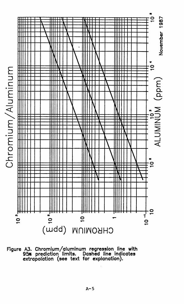
USING.THE INTERPRETIVE TOOL

Model figures with regression lines and prediction limits are

presented in the Appendix. The figures are constructed on a

log-log scale to facilitate plotting; absolute metal

concentrations can be plotted on the figures without the

necessity of loglo-transformation. These figures can be -

reproduced and routinely used to determine whether samples from

Florida estuarine sediments are enriched with metals. To do -

this, a mean value of each metal (derived from replicate or--

triplicate values) at a station is calculated and points

representing corresponding metal and aluminum values are plotted _

on the appropriate figures. The sediment is judged to be natural

or "metal-enriched" depending on where the points lie relative to -

the regression lines and prediction limits. If a point falls-

within the prediction limits, then the sediment metal

concentration is within the expected natural range. If a point -

falls above the upper prediction limit, then the sediment is

considered to be metal- enriched. Prior to making a -

determination of "enrichment", however, the accuracy of the-

analytical results should be confirmed, since an unusual point

can also be indicative of procedural errors. Furthermore, since -

the results are being evaluated with respect to a 95% prediction

limit, some points from "clean" stations will lie outside the -

prediction limit. The farther from the prediction limit, the

greater the likelihood that the sample does indeed come from a-

metal-enriched sediment. Also, greater distance above the-

prediction limit indicates a greater degree of enrichment.

-

30

-

-

-

-

-

-

-

-

-

-

-

-

-

Points that lie closely above the upper prediction limit must be

interpreted in light of available ancillary information about

possible sources of metal contamination and information from

other nearby stations. Likewise, some points from "clean"

sediments will fall below the lower prediction limit. Points

that are far below the lower prediction limit should be

considered suspect and examined for analytical errors.

APPLICATIONS OF THE INTERPRETIVE TOOL

The interpretive tool using metal and aluminum relationships

allows results of sediment chemical analyses to be used for a

variety of environmental information needs, including:

1. Distinauishinu natural versus enriched metals

concentrations in coastal sediments. The degree of

enrichment can also be estimated based on the deviation

from the expected natural range.

2. Comoarinq metal concentrations within an estuary.

Absolute metal concentrations in coastal sediments will

vary depending on many factors, including sediment grain

size, mineralogy, and anthropogenic metal sources.

Normalizing metals to the reference element, aluminum,

allows comparisons of metal concentrations among sites

within an estuary.

3. Comvarinca investiaative results from different

estuaries. By normalizing metal concentrations to

aluminum, an assessment of relative metal enrichment

levels can be made, allowing estuaries to be ranked

according to specific metal enrichment problems.

31

4. Trackinq the influence nf. a pollution source. As

illustrated in the next section, it is possible to

determine the extent of metal-enriched sediments.

Delineation of the extent of metal-enrichment can help

focus attention on real, rather than perceived, problems.

5. Monitorinq trends in metal concentrations Over time.BY

periodically examining sediments at permanent sampling

stations or along known pollution gradients, the

technique may provide a much-needed device for

cost-effective monitoring of the overall "pollution

climate" of estuaries.

6. Determinina nrocedural u laboratory errors. The

location of points on the metal/aluminum figures can

signal possible errors, which could include sample

contamination in the field or laboratory, as well as

analytical or reporting errors.

7. Screeninq tool to promote cost-effective u of elutriate

or other tests. A variety of tests (eg., elutriate,

bioassay) are used to demonstrate potential release to

the water column or toxicity of metals in sediments. The

interpretive tool described here can be used to reduce

the time and cost of testing by screening sediments and

selecting for further testing only those whose metal

concentrations exceed expected natural ranges. Testing

can be limited to the specific metals determined to be

enriched during the screening process.

-

-

-

-

-

-

-

-

-

-

32

LIMITATIONS w THE INTERPRETIVE TOOL

.-

-

-

-

_

-

-

-

-

-

.-

-

__

The approach presented in this document provides an

interpretive tool for evaluating metals concentrations in

estuarine sediments. Use of the tool requires knowledge of local

conditions and the application of professional judgement and

common sense. The following points should be kept in mind when

using this interpretive tool.

1) The interpretive tool is useless without reliable data.

Results from single, non-replicated samples should never be

used. Ideally, sediment samples should be collected in

triplicate. If budget constraints dictate analysis of only

duplicate samples, the third sample should be archived. In the

event of a disparity in the results of replicate analyses, the

archived sample should be retrieved and analyzed to resolve the

problem.

2) Sediment metals must be carefully analyzed using

techniques appropriate for saline conditions and capable of

providing adequate detection limits. Because naturally-occurring

aluminum and other metals are tightly bound within the

crystalline structure of the sediment minerals, the methods for

metals analyses must include complete sediment digestion. If

aluminum is not completely released by a thorough digestion,

metal to aluminum ratios may appear to be unusually high.

3) Mercury presents special problems, both in the laboratory

and in the interpretation of results. Since mercury is more

volatile than the other metals, a different digestion procedure,

employing a lower temperature than for the other metals, must be

used. Also, natural mercury concentrations are very near routine

33

_

analytical detection limits, where precision and accuracy are

reduced. Furthermore, mercury's apparent weak inverse

relationship with aluminum precludes the use of aluminum as a

reference element.

To deal with mercury, assume that the maximum mercury value

in the "clean" sediment data set (0.21 ppm mercury) represents

the maximum mercury concentration to be found in natural

sediments of Florida. For the purpose of evaluating sediment

samples, those containing less than 0.21 ppm mercury can be-

considered as typical of clean sediments. Samples with greater

than 0.21 ppm mercury should be suspected as being enriched and

should be interpreted similarly to those other metals that fall -

outside of the 95% prediction limits.

4) Similar to mercury, natural concentrations of cadmium are -

also low and are near normal analytical detection limits.-

Because of this, analytical precision and accuracy are reduced

and special care must be taken to obtain accurate laboratory -

results.

5) Aluminum concentrations in the data set from which these -

guidelines were prepared ranged from 47 to 79,000 ppm. The data

-set is, to the extent possible in this project, representative of

various types of natural "clean" sediments found in Florida

estuaries. The majority of samples recovered from Florida

estuarine sediments will have aluminum concentrations within

range.

-

this _

Some clay-rich sediments, however, especially in northwest-

Florida, may contain aluminum concentrations exceeding 79,000-

ppm. Kaolinite, illite (muscovite), montmorillonite, and

-

34

-

-

-

-

-

-

-

-

-

chlorite, four commonly occurring marine clays, contain aluminum

concentrations of approximately 21%, 20%, 15%, and lo%,

respectively (calculated based on chemical formulas for the clay

minerals given in Riley and Chester, 1971). Theoretically,

therefore, the maximum aluminum concentration in a natural marine

sediment is about 210,000 ppm (21%), if the sediment is composed

of pure kaolinite. Since sediments are not pure clay, the

aluminum concentration in estuarine sediment samples should be

considerably less than this theoretical maximum and only in a few

instances should aluminum concentrations exceed 100,000 ppm (10%

aluminum). Any samples containing greater than 100,000 ppm

aluminum should be examined carefully for evidence of

contamination or analytical error.

In order to extend the applicability of the interpretive tool

to sediments containing aluminum in excess of 79,000 ppm, the

regression lines and prediction limits have been extrapolated out

to an aluminum concentration of 100,000 ppm. (Since the

calculations were done on loglO-transformed data, the

extrapolation was from 4.9 to 5.0 log units. Aluminum values in

the'data set ranged from 1.7 to 4.9 log units.) The

extrapolations are indicated on the figures by dashed lines.

This is considered to be a reasonable approach. However, any

interpretations based on the extrapolated lines should be

qualified with a statement acknowledging that the data in

question exceeds the range of the "clean" data set from which

these guidelines were prepared.

6) During the construction of the "trimmed clean" data set,

some points containing low aluminum values were removed from the

35

-

cadmium, lead, nickel, and zinc data. Since, however, the lowest

overall aluminum value was 47 ppm, the regression lines and

prediction limits for these four metals have been extrapolated

down to an aluminum value of 47 ppm. These extrapolations are

also indicated by dashed lines.

7) At stations where a metal's concentration exceeds the 95%

prediction limit, the metal must be considered "enriched". One

must not immediately assume, however, that a finding of

"enrichment" is indicative of a problem. There is a probability

that some samples from natural "clean" sediments will contain

metals whose concentrations exceed the 95% prediction limit.

Interpretation of metal concentrations using these metal to

aluminum relationships must also take into consideration sediment

grain size, mineralogy, coastal hydrography, and proximity to

sources of metals. In the following section are two examples of

the use of this metals interpretive tool.

-

EXAMPLES

-

The following two examples show how the interpretive tool is -

used in combination with ancillary information to evaluate metals

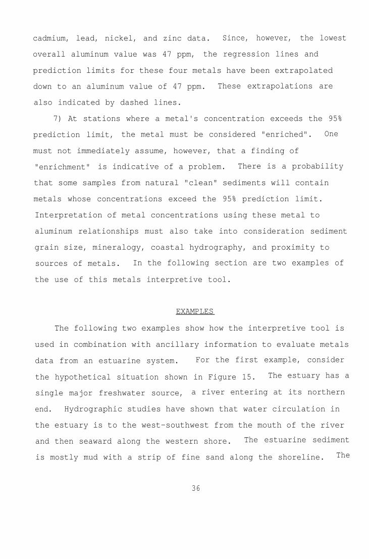
data from an estuarine system. For the first example, consider

the hypothetical situation shown in Figure 15. The estuary has a -

single major freshwater source, a river entering at its northern

end. Hydrographic studies have shown that water circulation in -

the estuary is to the west-southwest from the mouth of the river

and then seaward along the western shore. The estuarine sediment

is mostly mud with a strip of fine sand along the shoreline. The

-

36

-

River !j:.::‘.... .7::::.

. _. :..’

//

..:T”. :y::. ...:.. . .. . .::::.:.::

‘:::.::+:

I.2$ijs Fine Sand. . . . . . . :.

lssl Mud

Figure 15. Hypothetical estuary showing sampling stations andsediment grain size.

37

estuary is still in a "pristine" state with no known

anthropogenic sources of metal along its shores or in the river.

Sediments from Stations 1 9 were collected and analyzed for *

chromium.

Results of the chromium analyses are shown in Figure 16.

Several points are illustrated by these results. Chromium

concentrations vary with sediment grain size, being greatest at

the stations with finest sediment. However, despite the

-

differences in absolute chromium concentrations, Stations 1, 3, -

4, 5, 6 and 8 all have metal values falling within the natural-

range. Station 2, although statistically enriched with chromium,

does not in practice appear indicative of any problem since, it -

is only slightly above the prediction limit and since the

surrounding stations (Sta. 1, 3, 4, 5, 6) all have chromium -

concentrations within the natural range. Stations 7 and 9 each-

have chromium values that lie far outside the 95% prediction

limit. The chromium value from Station 7 is unusually low which, -

since the aluminum value is reasonable given the aluminum

concentrations of the other similar stations, indicates a -

possible laboratory error. There are at least three possible

explanations for the anomalously high chromium value at Station-

9: 1) the sample was contaminated, 2) there was a laboratory

error, or 3) there is an unusual and unknown source of chromium

in this area. Given the conditions described for this example, _

the first two possibilities are most likely. To examine these,

one needs to review the field data sheets (to identify any field -

sampling problems), laboratory logbooks, and the original raw-

data. Occasionally, spurious data from a single replicate can

-

38

-

-

-

-

-

-

F”” ’ ’ I”” ’ ’ ’ ’ I”“’ ’ ’ ’ I”” ’ ’ ’ ’n m

0 0 0 F iF

-0

- C

(udd) WniWOtlH3 -

Figure 16. Chromium results from hypotheticalestuarinq sampling stations shown in Figure 15.

-

-

- 39

greatly alter mean concentrations at a site, so the data should

be examined for outliers. If the latter two possibilities can be

ruled out, then further investigations to determine the source of

the chromium are in order.

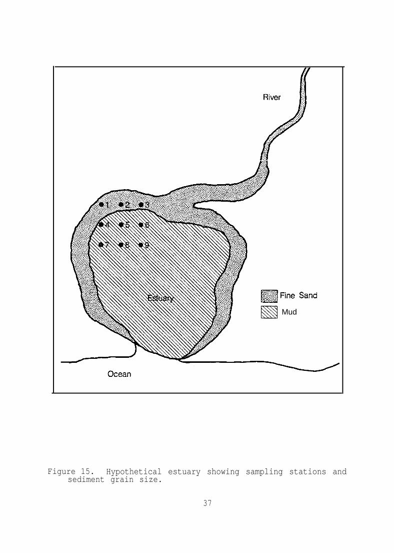
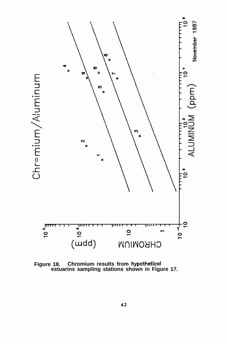
For the second example, consider the situation shown

Figure 17. Conditions are the same in this hypothetical

in

estuary

as they were for the previous example, except for the presence of -

an urbanized area in the northwest portion of the system.

Drainage from the urban area enters the estuary and is a -

potential source of metal contamination. Sediment samples are-

taken at the locations indicated and analyzed for chromium;

results of the analyses are plotted in Figure 18. -

Based on the information described above, the extent of elevated

chromium concentrations is indicated by the dashed line in Figure -

17. Chromium from the pollution

accumulating in the sediments at

concentrations at these stations

interval and, assuming they have

source appears to be

stations 1, 2, and 4. Chromium -

lie outside the 95% confidence -

been checked for errors, can be

considered indicative of chromium-enriched sediment. Stations 3, _

5, 6, 7, 8 do not have elevated chromium levels and thus appear

to be outside the range of influence of the chromium source.-

Note that the absolute concentration of chromium at Station 1 is-

less than that at Stations 5 and 6 but Station 1 is considered to

be enriched with chromium. Station 9 has a chromium value just _

outside the 95% prediction limit but given its location and the

metal concentrations at the surrounding stations, the station is

judged to be unpolluted.

40

-

-

-

-

-

-

-

-

-

-

DevelopedArea

Ocean

Figure 17. Hypothetical estuary showing metal source, samplingstations, and sediment grain size. Dashed lineindicates extent of elevated chromium concentrations.

41

E3c.-E3

E2.-

E0

I-“’ ’ ’ ’ I”“’ ’ ’ ’ I”“’ ’ ’ ’ I”“’ ’ ’ ’ 0n m 7

P

0 0- &) wn’ivw~H3- F

Figure 18. Chromium results from hypothetkalestuarins sampling stations shown in Figure 17.

-

-

-

-

-

-

-

-

-

-

-

-

-

-

42

-

REFERENCES-

-

-

-

-

-

-

-

-

-

-

Duce, R. A., G. L. Hoffman, B. J. Ray, I. S. Fletcher, G. T.Wallace, S. R. Tiotrowicz, P. R. Walsh, E. J. Hoffman, J. M.Miller, and J. L. Heffter. 1976. Trace metals in the marineatmosphere: sources and fluxes. In H. L. Windom and R. A.Duce (ea.), Marine pollutant transfer. Lexington Books,Lexington, Massachusetts.

FDER/OCM. 1984. Deepwater ports maintenance dredging anddisposal manual. Florida Department of EnvironmentalRegulation, Tallahassee.

FDER/OCM. 1986a. Geochemical and statistical approach forassessing metals pollution. Florida Department ofEnvironmental Regulation, Tallahassee.

FDER/OCM. 198633. Guide to the interpretation of reported metalconcentrations in estuarine sediments.

Filliben, J. J. 1975. The probability plot correlationcoefficient test for normality. Technometrics 17: 111 -117.

Goldberg, E. D., J. J. Griffin, V. Hodge, M. Koide, and H.Windom. 1979. Pollution history of the Savannah Riverestuary. Environmental Science and Technology 13: 588 - 594.

Martin, J. M. and M. Whitfield. 1983. The significance of theriver inputs to the ocean. In C. S. Wong, E. Boyle, K. W.Bruland, J. D. Burton, and E. D. Goldberg (ea.), Trace metalsin seawater. Plenum Press, New York.

Riley, J. P., and R. Chester. 1971. Introduction to marinechemistry. Academic Press, New York.

Ryan, T. A., B. L. Joiner, and B. F. Ryan. 1982. Minitabreference manual. Duxbury Press, Boston.

Sokal, R. R. and F. J. Rohlf. 1969. Biometry: the principlesand practice of statistics in biological research. W. H.Freeman and Company, San Francisco.

Taylor, S. R. 1964. Abundance of chemical elements in thecontinental crust: a new table. Geochimica et CosmochimicaActa 28: 1273 - 1286.

Taylor and McLennan. 1981. The composition and evolution of thecontinental crust: rare earth element evidence fromsedimentary rocks. Philosophical Transactions of the RoyalSociety of London 301A: 381 - 399.

-

43

-

Trefry, J. H., S. Metz, and R. P. Trocine. 1985. The decline inlead transport by the Mississippi River. Science 230: 439 -441.

Trefry, J. H. and B. J. Presley. 1976. Heavy metals insediments from San Antonio Bay and the northwest Gulf ofMexico. Environ. Geol. 1: 283 - 294.

Turekian, K. K. and K. H. Wedepohl, 1961. Distribution ofthe elements in some major units of the earth's crust.Geological Society of America Bulletin 72: 175 - 192.

USEPA. 1982. Methods for chemical analysis of water andwastes. EPA 600/4-79-020. Environmental Monitoring andSupport Laboratory, U. S. Environmental Protection Agency,Cincinnati, Ohio.

-.

-

Wilkinson, L. 1986. SYSTAT: the system for statistics.Systat, Inc., Evanston, Illinois.

44

-

-

-

-

-

-

-

-

-

-

-

-

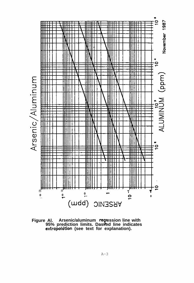
APPENDIX

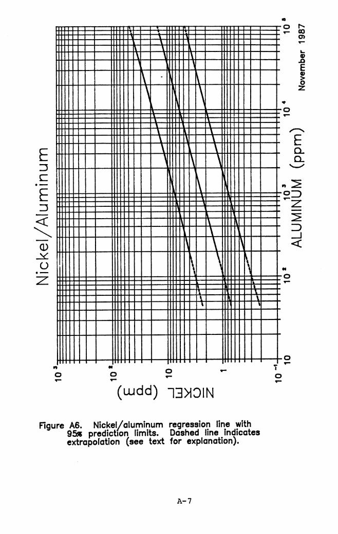
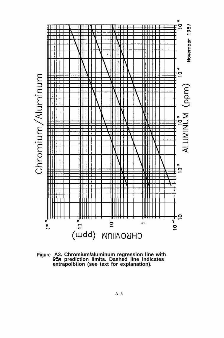
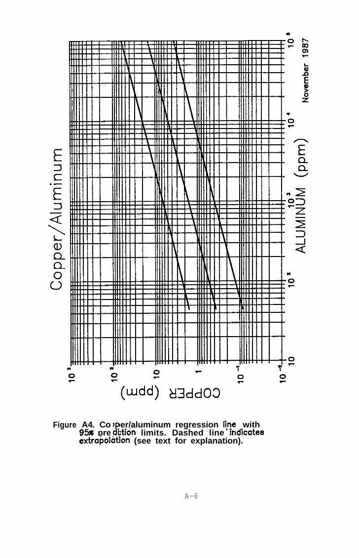
This appendix contains blank metal/aluminum figures with

regression lines and 95% prediction limits. Extrapolated

portions of the lines are represented by dashed lines (see

explanation in text). Metals data can be plotted on these

figures as described in the text for assessment of metal

enrichment in estuarine sediments.

-

-

-

-

-

-

-

-

-

-

A-l

Figures

FIGURE Al. Arsenic/aluminum regression line with95% predictionlimits . . . . . . . . . . . . . . A-3

FIGURE A2. Cadmium/aluminum regression line with95% prediction limits . . . . . . . . . . . . . . A-4

FIGURE A3. Chromium/aluminum regression line with95% prediction limits . . . . . . . . . . . . . . A-5

FIGURE A4. Copper/aluminum regression line with 95%prediction limits . . . . . . . . . . . . . . . . A-6

FIGURE A5. Nickel/aluminum regression line with 95%prediction limits . . . . . . . . . . . . . . . . A-7

FIGURE A6. Lead/aluminum regression line with 95%prediction limits . . . . . . . . . . . . . . . . A-8

FIGURE A7. Zinc/aluminum regression line with 95%prediction limits . . . . . . . . . . . . . . . . A-9

--.

-

-.

-

--

A-2

-

--

-

-

-

-

-

-

-

-

-

-

-

n rr0 0 0

P- F

Cudd)

. . . , . . . . . . . . I’.. .

F 70F

3lN3SW0

Figure Al. Arsenic/aluminum re ression line with95% prediction limits. Das ed line indicates7lextrapolbtion (see text for explanation).

A-3

I I

Ill1 I ll~ll I I llJ,#p I I ll~l II ’ ‘0

c a OF0e

Figure

c I

0 b bC C F

(wdd) tinlwav3

A2. Cadmium/aluminum regression. live with95% prediction limits. Dashed line lndtcatesextrapolbtion (see text for explanation).

-

-

-

-

.-

-

A-4-

-

-

-

-

-

-

-

+!!! : II

nT0P

Figure A3. Chromium/aluminum regression line with95% prediction limits. Dashed line indicatesextrapolbtion (see text for explanation).

-

A-5

E

Q\La,a,CL0

c)

Figure

(U’dd) Hdd03

A4. Co per/aluminum regression li,ne. with95% pre i&ion limits. Dashed line Indicates(Pextrapolbtion (see text for explanation).

_...

-

-

-

-

-

-

A-6-

-

-

-

-.

-

-

-

-

E3t.-

E3

Q\a>v0.-Z

-(wdd)

Figure A6. Nickel/aluminum95% prediction limits.extrapolation (see text

13)131N

regression line withDashed line indicatesfor explanation).

A-7

E3s.-E3

Figure A5. Lead/aluminum regression line with9% prediction limits. Dashed line indicatesextrapolbtion (see text for explanation).

-

-

-

-

A-8

-

-

-

- E3c.-E3

-

-

-

-

Figure A7. Zinc/aluminum re ression line with95s prediction limits. 8ashed line indicatesextrapolbtion (see text for explanation).

A-9