a guide to the use of: excel 2010 - sdpbc web cms · pdf filemicrosoft excel version 1 i a...

Microsoft Excel Version 1

i

A Guide to the use of:

Excel

2010

Developed by:

Staff Development

Technical Operations

Information Technology

School District of Palm Beach County

Version 1

i

Table of Contents

1 INTRODUCTION ................................................................................................ 1-1

1.1 OVERVIEW ............................................................................................................................... 1-1

1.2 13B. OPENING EXCEL ................................................................................................................... 1-1

1.3 SCREEN LAYOUT ...................................................................................................................... 1-2

1.4 QUICK ACCESS TOOLBAR ......................................................................................................... 1-2

2 RIBBON, TABS AND GROUPS......................................................................... 2-4

2.1 RIBBON .................................................................................................................................... 2-4

2.2 TABS ....................................................................................................................................... 2-4

2.2.1 File Tab .............................................................................................................................. 2-5 2.2.1.1 Info ............................................................................................................................................................. 2-5 2.2.1.2 Recent ......................................................................................................................................................... 2-6 2.2.1.3 Print ........................................................................................................................................................... 2-6 2.2.1.4 Options ....................................................................................................................................................... 2-6

2.2.2 Home Tab .......................................................................................................................... 2-7 2.2.3 Insert Tab ........................................................................................................................... 2-7 2.2.4 Page Layout Tab ............................................................................................................... 2-8 2.2.5 Formulas Tab..................................................................................................................... 2-8 2.2.6 Data Tab ............................................................................................................................ 2-8 2.2.7 Review Tab ........................................................................................................................ 2-8 2.2.8 View Tab ............................................................................................................................ 2-9

2.3 GROUPS ................................................................................................................................ 2-10

3 WORKBOOK ..................................................................................................... 3-1

3.1.1 New Workbook .................................................................................................................. 3-1

3.2 SAVING A WORKBOOK ............................................................................................................. 3-1

3.3 FORMULA BAR ......................................................................................................................... 3-2

4 3BWORKSHEET .................................................................................................. 4-1

4.1 SELECTING A CELL ................................................................................................................... 4-2

4.1.1 56BUsing the Mouse ................................................................................................................ 4-2 4.1.2 57BName Box .......................................................................................................................... 4-2

4.2 ENTERING DATA ....................................................................................................................... 4-3

4.2.1 58BText .................................................................................................................................... 4-3 4.2.2 59BNumbers ............................................................................................................................ 4-3

4.3 EDITING A CELL ........................................................................................................................ 4-4

4.4 FIND, MOVE OR COPY CELLS .................................................................................................... 4-4

4.4.1 60BFind .................................................................................................................................... 4-4 4.4.2 61BDrag and Drop ................................................................................................................... 4-4 4.4.3 62BCopy and Drop .................................................................................................................. 4-5 4.4.4 Cut and Paste .................................................................................................................... 4-5 4.4.5 64BCopy and Paste ................................................................................................................. 4-5 4.4.6 65BInsert Copied Cells ............................................................................................................ 4-5

4.5 FILL HANDLE .......................................................................................................................... 4-5

4.5.1 66BText .................................................................................................................................... 4-5

Version 1

ii

4.5.2 67BNumbers ............................................................................................................................ 4-6 4.5.3 68BDates ................................................................................................................................. 4-6 4.5.4 69BFormulas/Functions ........................................................................................................... 4-7 4.5.5 Auto Fill .............................................................................................................................. 4-7 4.5.6 Fill non-adjacent cells ........................................................................................................ 4-8

4.6 TRANSPOSING CELLS ............................................................................................................... 4-8

4.7 CELL REFERENCES .................................................................................................................. 4-9

5 4BFORMULAS, FUNCTIONS ................................................................................ 5-1

5.1 29BFORMULAS ............................................................................................................................... 5-1

5.1.1 70BManual Entry...................................................................................................................... 5-1

5.2 FUNCTIONS .............................................................................................................................. 5-2

5.2.1 71BAuto Sum ........................................................................................................................... 5-2

6 5BFORMATTING .................................................................................................... 6-1

6.1 FORMATTING ............................................................................................................................ 6-1

6.1.1 72BBasic Formatting ................................................................................................................ 6-2 6.1.2 73BAutoFormat ........................................................................................................................ 6-3 6.1.3 74BColumn & Row Sizing ........................................................................................................ 6-3

6.1.3.1 Controlling Row Height.............................................................................................................................. 6-3 6.1.4.1 Controlling Column Width ......................................................................................................................... 6-4

6.1.5 75BInsert Blank Rows or Columns .......................................................................................... 6-4 6.1.5.1 Inserting a Single Row or Column .............................................................................................................. 6-4 6.1.5.2 Inserting Multiple Rows or Columns .......................................................................................................... 6-5

6.1.6 76BStyle ................................................................................................................................... 6-7 6.1.7 77BOptions .............................................................................................................................. 6-7 6.1.8 78BChange Text Case ............................................................................................................. 6-8 6.1.9 79BWord Wrap ......................................................................................................................... 6-8

6.1.9.1 Text ............................................................................................................................................................. 6-8 6.1.9.2 Titles ......................................................................................................................................................... 6-9

6.2 CONDITIONAL FORMATTING .................................................................................................... 6-10

7 6BCHARTS ............................................................................................................. 7-1

7.1 INSERT A CHART ...................................................................................................................... 7-1

7.1.1 Select Data ........................................................................................................................ 7-1 7.1.2 Charts Group ..................................................................................................................... 7-2

7.1.2.1 Chart Type ................................................................................................................................................. 7-2 7.1.2.2 Chart Terms ................................................................................................................................................ 7-3 7.1.2.3 Chart Tools ................................................................................................................................................. 7-3

7.2 EDIT ........................................................................................................................................ 7-5

7.2.1 Changing the Chart Size ................................................................................................. 7-5 7.2.2 Moving ............................................................................................................................... 7-5 7.2.3 Deleting .............................................................................................................................. 7-5 7.2.4 Adding Data ....................................................................................................................... 7-6

7.2.4.1 Change Data ............................................................................................................................................. 7-6 7.2.4.2 New Data ................................................................................................................................................. 7-6

8 7BWORKING WITH EXCEL ................................................................................... 8-1

8.1 SPELL CHECKING ..................................................................................................................... 8-1

8.2 CHANGING SHEET NAMES ........................................................................................................ 8-1

8.3 MOVE A WORKSHEET ............................................................................................................... 8-2

8.4 COPYING ACROSS WORKSHEETS .............................................................................................. 8-2

8.5 LINKING FILES .......................................................................................................................... 8-3

Version 1

iii

8.6 FREEZE PANES ........................................................................................................................ 8-3

8.7 FILTERING DATA ....................................................................................................................... 8-4

8.8 SORTING.................................................................................................................................. 8-5

8.8.1 86BSimple Sorts ...................................................................................................................... 8-5 8.8.2 87BSorting by Multiple Columns .............................................................................................. 8-5

9 8BPRINTING .......................................................................................................... 9-1

9.1 WORKSHEET ............................................................................................................................ 9-1

9.1.1 88BPage Setup. ....................................................................................................................... 9-2 9.1.2 89BManual Page Breaks ......................................................................................................... 9-3

9.2 WORKBOOK ........................................................................................................................... 9-3

10 10BONLINE RESOURCES ................................................................................. 10-1

10.1 48BTRAINING ............................................................................................................................... 10-1

10.2 EXCEL HELP SYSTEM ............................................................................................................. 10-3

10.3 TRAINING MANUAL ................................................................................................................. 10-3

11 11BSAMPLE EXCEL SPREADSHEETS ............................................................ 11-1

11.1 BLUE SKY AIRLINES ................................................................................................................ 11-1

11.2 AMORTIZATION SCHEDULE ...................................................................................................... 11-2

11.2.1 90BTable 1 ........................................................................................................................ 11-2 11.2.2 91BTable 2 ........................................................................................................................ 11-3

Version 1

iv

Updates Version 1

Baseline release version

Version 1

i

This page is blank


1-1

1 Introduction

1.1 Overview

Microsoft Excel is a spreadsheet program that allows the user to organize data, complete calculations, make decisions, graph data, develop professional looking reports, publish organized data to the Web, and access real-time data from Web sites. It can be used in conjunction with other programs such as MS Word, MS Access as well as software packages such as PeopleSoft and SAP to produce specific reports and report formats.

The three major parts of Excel are:

1. Worksheets. Worksheets allow the user to enter, calculate, manipulate, and analyze data such as numbers and text. Note that the term worksheet is used interchangeably with the term spreadsheet.

2. Charts. Charts are pictorial representations of data. Excel can create/draw a variety of two-dimensional and three-dimensional charts.

3. Databases. Databases are used to manage data. For example, once data is entered onto a worksheet, Excel can manage it as though it were a database. It can sort the data, search for specific data, and select data that meets a criterion.

1.2 13B. Opening Excel To run Excel on your computer: “Start” >> “Programs” >> “Microsoft Office” >> “Microsoft Office Excel 2010.”

If there is an icon of Microsoft Excel available on your desktop (shaped like a square with a "X"),

you can open up the program by double-clicking it, as well.


1-2

1.3 Screen Layout

1.4 Quick Access Toolbar

In the upper left corner of the window, there is an area called the Quick Access Toolbar. This area contains several of the most used buttons in Office applications –

Save, Undo, Redo, Print and Print Preview. This toolbar can be customized by adding and removing as many Quick Access button choices as needed.

Ribbon

Tabs

Groups

View choices

Worksheet


1-3

To customize the Quick Access Toolbar,

Click on the small arrow to the right of the bar.

If the ability to draw a table were to be added to the toolbar;

o lick the Draw Table Entry

o A check mark will be added to the left of the Draw Table entry and the Draw Table icon will be added

to the Quick Access Toolbar.

To remove buttons from the Quick Access Toolbar:

o RIGHT click on the button to be removed

o Choose Remove from Quick Access Toolbar.


2-4

2 Ribbon, Tabs and Groups

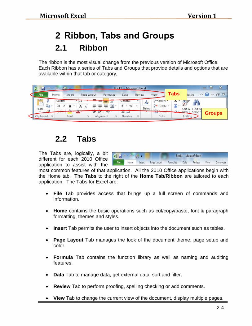
2.1 Ribbon The ribbon is the most visual change from the previous version of Microsoft Office. Each Ribbon has a series of Tabs and Groups that provide details and options that are available within that tab or category,

2.2 Tabs The Tabs are, logically, a bit different for each 2010 Office application to assist with the most common features of that application. All the 2010 Office applications begin with the Home tab. The Tabs to the right of the Home Tab/Ribbon are tailored to each application. The Tabs for Excel are:

File Tab provides access that brings up a full screen of commands and information.

Home contains the basic operations such as cut/copy/paste, font & paragraph formatting, themes and styles.

Insert Tab permits the user to insert objects into the document such as tables.

Page Layout Tab manages the look of the document theme, page setup and color.

Formula Tab contains the function library as well as naming and auditing features.

Data Tab to manage data, get external data, sort and filter.

Review Tab to perform proofing, spelling checking or add comments.

View Tab to change the current view of the document, display multiple pages.

Tabs

Groups


2-5

2.2.1 File Tab

The File tab brings up a full screen of commands and information. Microsoft calls this screen the Backstage View. This tab is new to this version of MS Office. The Backstage View provides access to the normal File functions such as Save, Save As, Open, etc. as well as several options

2.2.1.1 Info

The Info option provides two sections that give the user the ability to see the details related to the document that is currently open. The first section contains a section that supplies information about the document.

The document Read-Only.

Compatibility issues exist.

The document is not protected.

Issue to check if the document is to be shared. The document versions that have been auto-saved and therefore accessible to the user. The second section displays the properties related to size and number of words as well as the date created, modified and last printed.


2-6

2.2.1.2 Recent

The Recent option displays recent documents that have been accessed as well as recent places (files or folders) that have been accessed. Documents or Places can be ‘pinned’ to the list by clicking on the push-pin next to each item. The item is now pinned to the list and will stay until the pin is again clicked to release it.

2.2.1.3 Print

The Print option displays the printer and settings that are available along with a sample of how the page will appear when printed.

2.2.1.4 Options

The Options screen provides access the settings that are used within MS Office. Many of these options are unique to the application (Word, Excel, etc.) that is currently being accessed. Most apply to all of MS Office applications. Caution should be taken when changing any of the system options.


2-7

2.2.2 Home Tab

This tab contains many of the most commonly used features. Popular commands

include:

Cut/Copy/Paste

Font & Paragraph Format (for more options)

Show & Hide Formatting (¶)

Themes & Styles

Find & Replace

2.2.3 Insert Tab

Many objects (tables, images, clipart, & Headers/Footers) you insert into your

Word document come with context-sensitive tabs which pop up when the item

is selected.

o Example: Picture Tools Tab (appears when you Insert a Picture)

The Picture Tools tab is another example of Office 2010’s content-sensitive hovering. You have and the ability to instantly preview image editing options, including:

Brightness

Contrast

Recolor (to Black & White or many other tones)

Add Borders & 3-D Effects

Rotate

Crop/Resize

Remove Background

o Example: Table Tools Tabs(appear when you Insert a Table)

Draw it out

Design (Colors & row styles)

Layout (Table manipulation, such as merge cells & add

rows/columns)

In Excel 2010, the Insert tab is also where you find various tools like:

o New feature: Screenshots!

o Headers/Footers (& page numbers)

o Page Breaks & Cover Pages

o Unusual Symbols (i.e. © or £)

o Hyperlinks (Where you can make a link like this instead of a link like this:

http://www.google.com)

o Sparklines

http://www.google.com/

http://www.google.com/


2-8

2.2.4 Page Layout Tab

As the title suggests, this tab contains groups and commands related to managing the

page layout of the document. It includes groups for:

Themes

Page Setup

Page Background

Paragraphs

Arrange

2.2.5 Formulas Tab

References that are required for a document can be setup or identified using the groups within this tab.

Footnotes & Endnotes

Table of Contents

Insert an Index

Automatically created based on Headers, or manually defined

Insert Caption

2.2.6 Data Tab

The Mailings Tab provides the mail-merge function within MS Word. It can be managed using the icons within the tab or by using the Step BY Step Mail Merge Wizard.

2.2.7 Review Tab

The Review Tab permits the user to access the tools needed to:

Spell Check

Word Count

Set Language

Track Changes (for documents that are edited by multiple people)

Compare the differences between 2 documents, even if the changes weren’t

tracked

Protect the document from further editing


2-9

2.2.8 View Tab

The View Tab provides a variety of document viewing options

Document Views

o Full Screen Reading is useful for reading long documents; it shows 2

pages at a time, & hides the ribbon.

Show/Hide:

o Rulers

o Gridlines

o Navigation Pane

Zoom

The Navigation Pane can be used when to initiate a search and to display navigation tabs when headings are created in a document using Heading Styles

The example on the right is a sample of this document with the navigation tabs turned on and displaying the Style/Section Headings. These tabs function as hyperlinks to the appropriate sections.


2-10

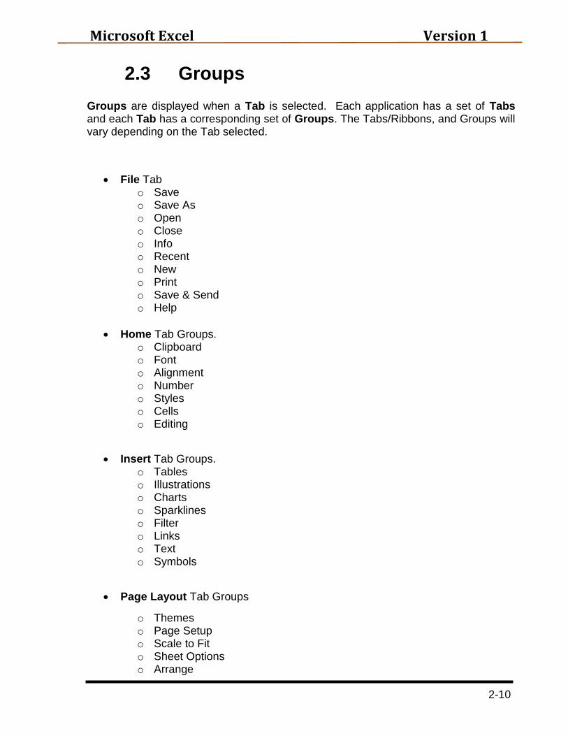
2.3 Groups Groups are displayed when a Tab is selected. Each application has a set of Tabs and each Tab has a corresponding set of Groups. The Tabs/Ribbons, and Groups will vary depending on the Tab selected.

File Tab o Save o Save As o Open o Close o Info o Recent o New o Print o Save & Send o Help

Home Tab Groups. o Clipboard o Font o Alignment o Number o Styles o Cells o Editing

Insert Tab Groups. o Tables o Illustrations o Charts o Sparklines o Filter o Links o Text o Symbols

Page Layout Tab Groups

o Themes o Page Setup o Scale to Fit o Sheet Options o Arrange


2-11

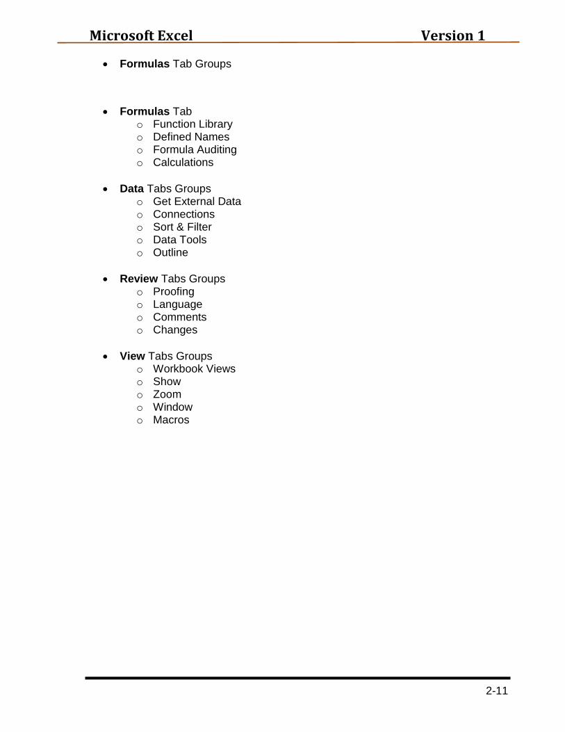
Formulas Tab Groups

Formulas Tab o Function Library o Defined Names o Formula Auditing o Calculations

Data Tabs Groups o Get External Data o Connections o Sort & Filter o Data Tools o Outline

Review Tabs Groups o Proofing o Language o Comments o Changes

View Tabs Groups o Workbook Views o Show o Zoom o Window o Macros


3-1

3 Workbook 3.1.1 New Workbook

Open up a new Excel workbook, do this by clicking on the File tab

Click on New

Excel 2010 will present a dialogue box to choose what type of new document.

The dialogue box contains a list of

templates. The user may select from an

installed template, or new office online

templates. The example depicts the

selection of a new blank workbook. Click on the Create button.

When Excel is started, it creates a new, empty workbook. Inside the workbook are sheets that are called worksheets. A new workbook will contain three worksheets that may be used. Each sheet has a name that is displayed on the sheet tab at the bottom of the workbook. As shown, Sheet1 is the worksheet displayed for workbook called Book1. If Sheet2 is clicked, then it would become the displayed active worksheet. Additional sheets in a workbook is limited by available memory (default is 3 sheets).

3.2 Saving a Workbook

1. Click the File tab. 2. Click the Save As function. NOTE: The Save As function

can save a copy of the Workbook under a new name. The Save function will save the workbook back to its original file. The original is lost!

3. Select the appropriate file folder for the saved workbook. 4. Enter the file name. 5. Click the Save button.


3-2

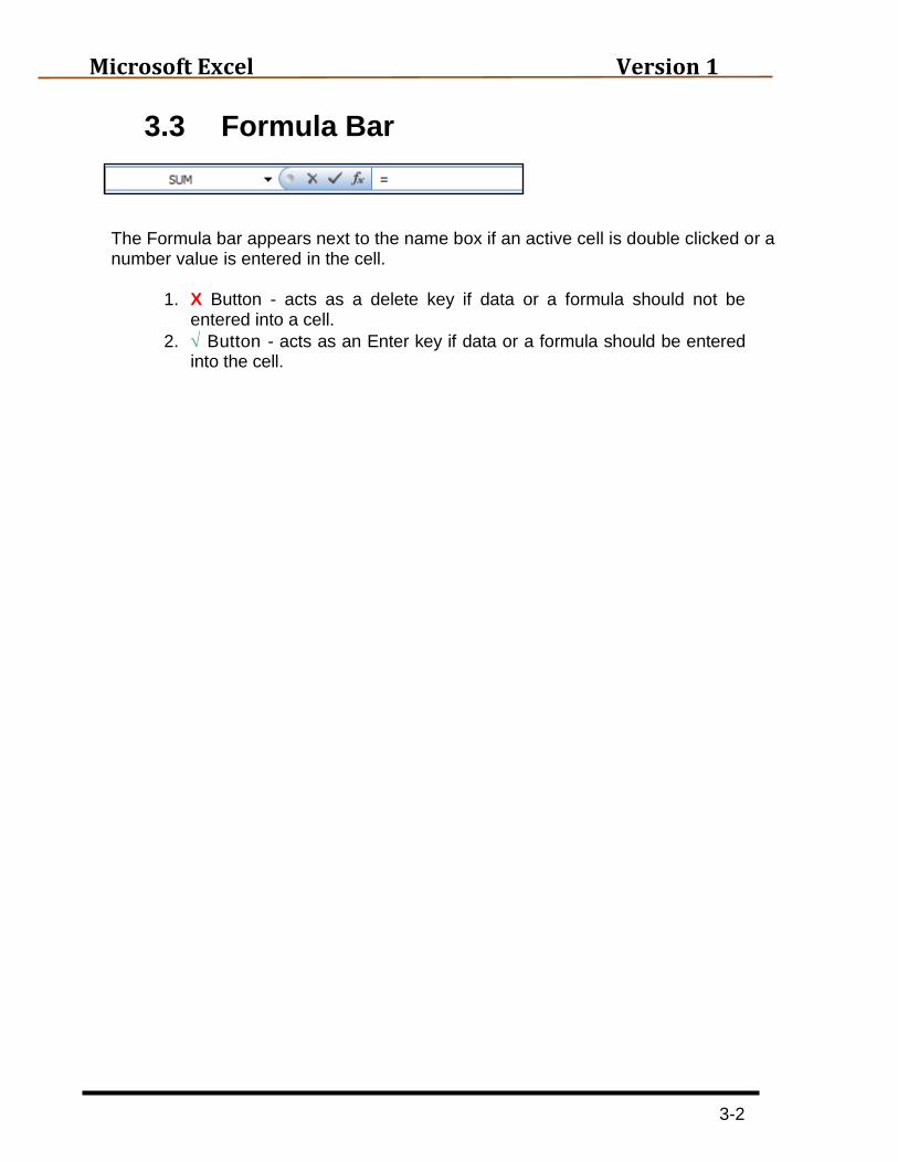
3.3 Formula Bar

The Formula bar appears next to the name box if an active cell is double clicked or a number value is entered in the cell.

1. X Button - acts as a delete key if data or a formula should not be entered into a cell.

2. Button - acts as an Enter key if data or a formula should be entered into the cell.


4-1

4 3BWorksheet

Cell – The intersection of a row and a column is a cell. This is the basic unit of a worksheet and is the place for entering text, numbers or formulas

Each worksheet in a workbook has 16,384 columns, and 1,048,576 rows. As shown in the figure at the right, when a spreadsheet is viewed, it only shows a small portion of the full worksheet. It is just a small window of the overall worksheet.

Cells are defined by the column heading letter and the row heading number. It is the cell reference and is a unique address for a cell. For example B3 identifies the cell at the intersection of column B and row 3.

Active Cell - The active cell is identified in the Name Box and has a heavy border around it. It is also highlighted in the row number heading and the column letter heading. The active cell is the only cell in which data may be entered.

Gridlines – Gridlines are horizontal and vertical lines on the worksheet that make it easier to see and to identify each cell on the worksheet.

Cursor – The mouse pointer (cursor) has the shape of a block plus sign whenever it is located in a cell on the worksheet. It turns into a block arrow whenever it is outside the worksheet or when cell content is dragged between rows or columns.

Scroll Bars

Sheet Tabs

Status Bar

Worksheet Window

Name Box with active cell reference

Heavy border surrounds active cell

Indicates cell A1 is active

Column heading letters

Gridlines Row heading numbers

16,384 Columns

1,048,576 Rows

Cursor Shapes


4-2

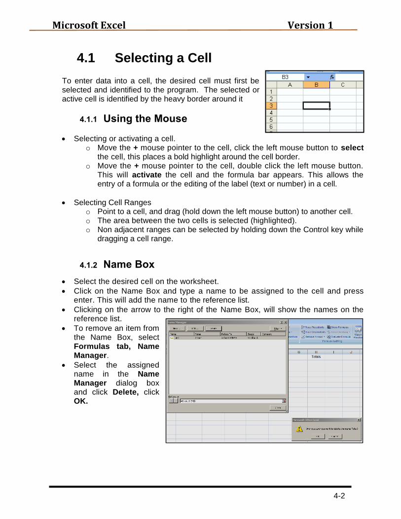
4.1 Selecting a Cell To enter data into a cell, the desired cell must first be selected and identified to the program. The selected or active cell is identified by the heavy border around it

4.1.1 56BUsing the Mouse

Selecting or activating a cell. o Move the + mouse pointer to the cell, click the left mouse button to select

the cell, this places a bold highlight around the cell border. o Move the + mouse pointer to the cell, double click the left mouse button.

This will activate the cell and the formula bar appears. This allows the entry of a formula or the editing of the label (text or number) in a cell.

Selecting Cell Ranges o Point to a cell, and drag (hold down the left mouse button) to another cell. o The area between the two cells is selected (highlighted). o Non adjacent ranges can be selected by holding down the Control key while

dragging a cell range.

4.1.2 57BName Box

Select the desired cell on the worksheet.

Click on the Name Box and type a name to be assigned to the cell and press enter. This will add the name to the reference list.

Clicking on the arrow to the right of the Name Box, will show the names on the reference list.

To remove an item from the Name Box, select Formulas tab, Name Manager.

Select the assigned name in the Name Manager dialog box and click Delete, click OK.


4-3

4.2 Entering Data

A spreadsheet cell can accept data in four different formats. They are: text, numbers, formulas, or functions. Detailed descriptions of the use of formulas and functions will be included in a later section of this manual.

4.2.1 58BText

Any set of characters entered into a cell that contains a letter, space or hyphen is considered text. A text entry can contain from 1 to 32,767 characters. Examples are: a social security number (999-99-9999), a title (Hours Worked), a single letter (A) or even a sentence (This is a short sentence). All text is aligned to the left side of the cell (left justified).

To enter text, click on the selected cell. That cell now has the heavy border and is identified as the active cell. Type the desired text into the formula bar. The text displays in the active cell and, if the text is longer than the cell width,

it will extend into the next cells. Click the Enter Box ( ) or another cell to complete the entry.

4.2.2 59BNumbers

Numbers can be entered into cells to represent amounts. Numbers can contain the following; 0 1 2 3 4 5 6 7 8 9 + - ( ) , / . $ % E e. Due to the need to align numbers based on a decimal point, all numbers are right justified in the cell. If a number must be entered as text, start the entry with an apostrophe ( ‘ ). The procedure for entering numbers is the same as entering text.

After the Enter key is clicked, the number is placed in the right justified position.

NOTE:

When a number does not fit in a cell (too long), Excel displays “#######”.


4-4

4.3 Editing a Cell

Activate the cell by moving the cursor to the cell.

If a cell contains previously entered data, typing into the selected cell replaces the information already in the cell. To edit the cell, place the cursor on the Formula Bar, or double click in the cell. Any portion of the label can be edited.

To cancel an edit, press Esc, or press the cancel button (X) on the formula bar.

Clearing an entry. o Select the cell or range of cells. o Press the delete key. o Or, select Home tab, Clear, click Clear Contents. There are number of

choices as to what should be deleted from the cell ex: Contents, Formats, Cell notes, or everything.

4.4 Find, Move or Copy Cells

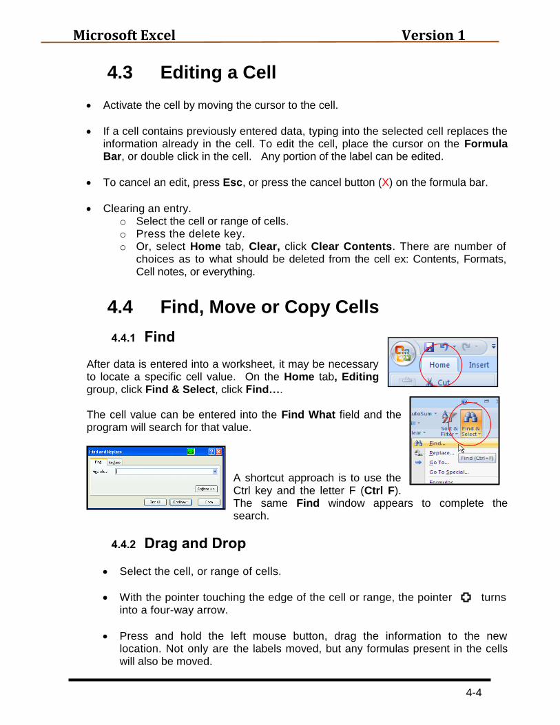
4.4.1 60BFind

After data is entered into a worksheet, it may be necessary to locate a specific cell value. On the Home tab, Editing group, click Find & Select, click Find…. The cell value can be entered into the Find What field and the program will search for that value.

A shortcut approach is to use the Ctrl key and the letter F (Ctrl F). The same Find window appears to complete the search.

4.4.2 61BDrag and Drop

Select the cell, or range of cells.

With the pointer touching the edge of the cell or range, the pointer turns into a four-way arrow.

Press and hold the left mouse button, drag the information to the new location. Not only are the labels moved, but any formulas present in the cells will also be moved.


4-5

4.4.3 62BCopy and Drop Use the same procedure as above while holding down the Control key on the

keyboard.

4.4.4 Cut and Paste

Select the cell or range to be moved.

Choose Home tab.

Select Cut.

Activate the new cell.

Click on the Paste arrow, select Paste, and the selected material will appear at the new location.

4.4.5 64BCopy and Paste

Same procedures as above except, in step 3, pick Copy.

The selected cell or range stays at the old location but the copy is transferred to the new site.

4.4.6 65BInsert Copied Cells

When moving cut or copied material into a row that already contains information, use the following procedure.

Select the row or range of rows to cut or copy.

Select Home tab, click cut or copy.

Select the row below which the cut or copied row(s) will be placed and right-click on that line.

Select Insert Copies Cells.

Press Esc key on keyboard to refresh screen.

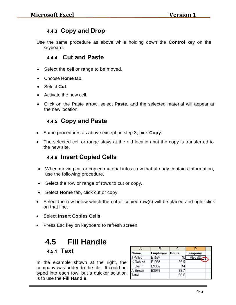
4.5 Fill Handle 4.5.1 66BText

In the example shown at the right, the company was added to the file. It could be typed into each row, but a quicker solution is to use the Fill Handle.


4-6

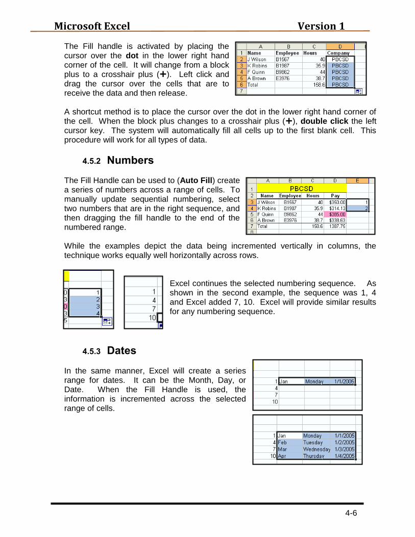
The Fill handle is activated by placing the cursor over the dot in the lower right hand corner of the cell. It will change from a block plus to a crosshair plus (). Left click and drag the cursor over the cells that are to receive the data and then release. A shortcut method is to place the cursor over the dot in the lower right hand corner of the cell. When the block plus changes to a crosshair plus (), double click the left cursor key. The system will automatically fill all cells up to the first blank cell. This procedure will work for all types of data.

4.5.2 67BNumbers

The Fill Handle can be used to (Auto Fill) create a series of numbers across a range of cells. To manually update sequential numbering, select two numbers that are in the right sequence, and then dragging the fill handle to the end of the numbered range. While the examples depict the data being incremented vertically in columns, the technique works equally well horizontally across rows.

Excel continues the selected numbering sequence. As shown in the second example, the sequence was 1, 4 and Excel added 7, 10. Excel will provide similar results for any numbering sequence.

4.5.3 68BDates In the same manner, Excel will create a series range for dates. It can be the Month, Day, or Date. When the Fill Handle is used, the information is incremented across the selected range of cells.


4-7

4.5.4 69BFormulas/Functions When the Fill Handle is used to Auto Fill a formula or function, Excel performs a ‘Relational’ copy. Excel copies the formula/function to the new cell(s) and adjusts it to meet the new row and/or column numbers. In the example, the computed values in the cells were converted to the formulas for clarity. The cell containing the formula (=c3*20) was copied to the three (3) cells below it. In each case, the cell referenced was incremented to the appropriate cell number.

4.5.5 Auto Fill Several options exist when using the fill handle. By right clicking to perform the fill action, a window appears displaying the options available. Options are available for formatting, filling or copying cells as well as management of days, months or trends. Each is highlighted based on the original cell value. For example:

Enter day in cell

Select the Fill Handle, right click, drag down

Cells are highlighted and a window appears.

Several options are available but two are unique for days of the week.

o Fill Days – will fill based on 7 day week

o Fill Weekdays – will fill based on 5 day work week.


4-8

4.5.6 Fill non-adjacent cells

While not employing the Fill Handle, a procedure

exists to fill non-adjacent cells with the same value.

Each cell is selected and then the value is typed into

the last cell selected.

Hold Cntl key down and select the desired cells.

In the last selected cell, type the value.

Hold down the Cntl key and press enter.

4.6 Transposing Cells

Frequently it becomes necessary to transpose cells in a work sheet. That is, to change them from columnar format to row format or row format to columnar. If this report was to be converted to show the titles in row 17 in a vertical format as row heading in column B.

Select the data to be transposed.

Right click to open the window that contains Copy

Copy the data

Select a cell on the spreadsheet that is not inside the area to be transposed.

Select the Paste Special button.

At the bottom of the window, select the Transpose block and click OK.


4-9

The rows and columns have now been transposed.

4.7 Cell References Microsoft Excel employs two methods of referencing cell addressing. They are Relative and Absolute.

R0Telative Cell Reference - In a formula, the address of a cell based on the relative position of the cell that contains the formula and the cell referred to. If you copy the formula, the reference automatically adjusts. A relative reference takes the form A1.)0T

0TAbsolute Cell Reference - In a formula, the exact address of a cell, regardless of the position of the cell that contains the formula. An absolute cell reference takes the form $A$1.)0T

When cells C2 and C3 are filled, the value from $B$1 remains constant.


5-1

5 4BFormulas, Functions

5.1 29BFormulas

Formulas are the basis for the calculations, models, and reports that can be built. Formulas always start with an equal sign ( = ) and be complex or as simple as the user needs.

5.1.1 70BManual Entry

1. Formula Properties.

All formulas begin with an equal sign (=). A formula is a sequence of values, cell references, names, functions, or operators contained in a cell that produces a new value from existing values.

When a formula is entered, the cell displays the value that results.

If a cell is selected, the Formula bar shows any underlying formula.

2. Editing a formula.

Procedure for editing a formula is the same as editing text.

Double click the cell; the formula will appear in the cell and on the formula bar.

The formula can be edited in the cell, or on the formula bar.

Pressing Control+' (the grave apostrophe, next to the exclamation point) will show all the formulas on one worksheet.

3. Arithmetic Operators.

The following are arithmetic operators used in Excel:

USymbol U UFunction

+ Addition - Subtraction * Multiplication / Division ^ Exponentiation % Percent when placed after a number

Examples. =1+2 Adds 1+2 =4/3 Divides 4 by 3 =2*3+8 Multiplies 2 by 3, then adds 8 =8+2*3 Multiplies 2 by 3, then adds 8 (see below) =3 ^2 Square 3 (3 x 3 = 9)


5-2

4. Order of Calculation.

An operation within parentheses takes precedence in calculations. After those, Excel performs exponential calculations, followed by multiplication and division. Addition and subtraction are the last items to be calculated. A simple memory tool is;

5.2 Functions

Excel contains a series of built-in formulas that are commonly used within the spreadsheet environment. They perform calculations or series of calculations based on preset rules. Functions are found on the Formulas tab, Function Library group. Functions must know what the starting values or arguments are in order to complete the calculation. There are hundreds of functions that are built-in to Excel to perform tasks such as SUM, AVERAGE and MAX. To perform the required calculations, the function requires input parameters or arguments. For example, to add the numbers 4,5,6 the formula =SUM(4,5,6) would be entered. If these values were in cells, the formula would be =SUM(A1,A2,A3). If the cells are contiguous, the formula would be expressed with the range of cells, =SUM(A1:A3). Each function will require a specific set of arguments to satisfy its rules.

5.2.1 71BAuto Sum

As columns of numbers are added to a spreadsheet, it is frequently necessary to sum the numbers either by column or by row. To accomplish this task, Excel includes a SUM function.

Please Parentheses ( )

Excuse Exponent ^

My Multiply *

Dear Divide /

Aunt Add +

Sally Subtract -


5-3

The AutoSum button is located on the Formulas tab or on the Home tab. To use this function

Identify the cell in which the sum is to be stored.

Once that cell has been identified as the active cell, then click the AutoSum

button ( ).

Excel puts a dotted line around the proposed range of cells to be summed, writes the formula for the sum in the formula box and displays the formula in the selected cell. Click Enter or the AutoSum button again to complete the transaction.

A range is a series of two or more adjacent cells in a column, row, or a rectangular group of cells. The value displayed in cell C6 is a ‘computed value’. It is the result of a formula or a function and is based on the values of the cells included in the range.


6-1

6 5BFormatting

6.1 Formatting The entry of data into a worksheet provides the basics for reporting. Formatting of the data and the appearance of the spreadsheet completes the job and improves readability. The figure shows a sample spreadsheet without formatting.

The second figure shows the impact of adding formatting to the spreadsheet.


6-2

6.1.1 72BBasic Formatting

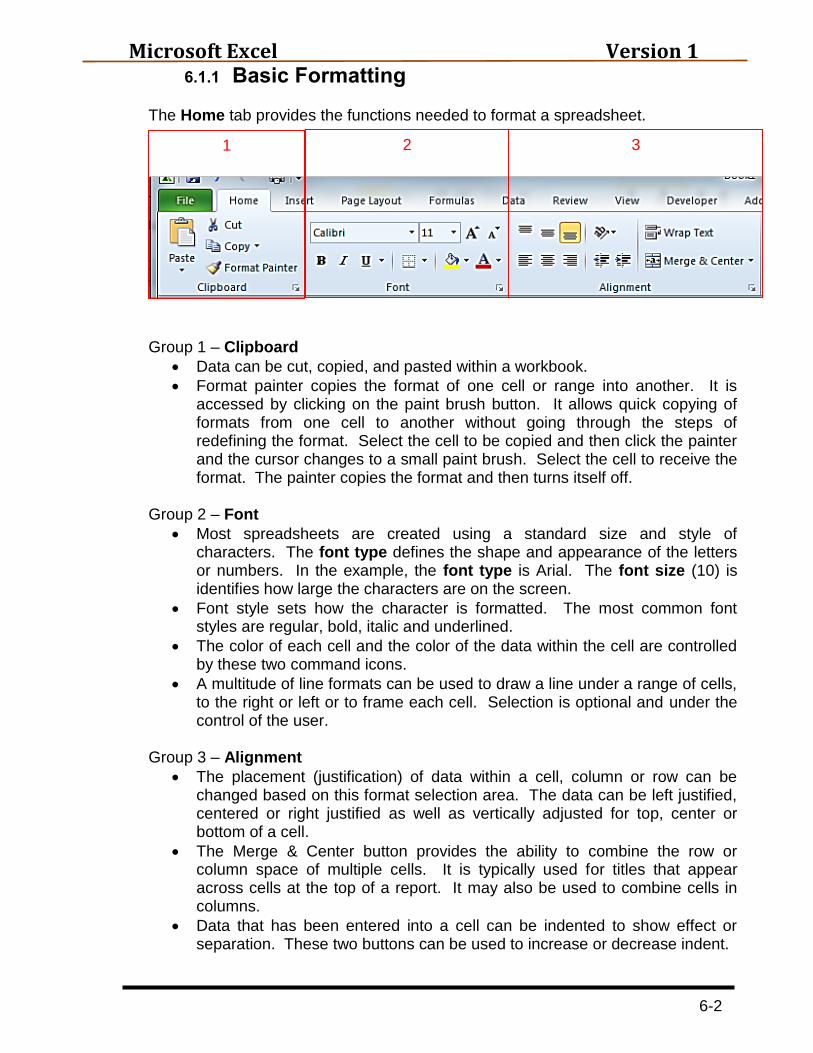
The Home tab provides the functions needed to format a spreadsheet.

Group 1 – Clipboard

Data can be cut, copied, and pasted within a workbook.

Format painter copies the format of one cell or range into another. It is accessed by clicking on the paint brush button. It allows quick copying of formats from one cell to another without going through the steps of redefining the format. Select the cell to be copied and then click the painter and the cursor changes to a small paint brush. Select the cell to receive the format. The painter copies the format and then turns itself off.

Group 2 – Font

Most spreadsheets are created using a standard size and style of characters. The font type defines the shape and appearance of the letters or numbers. In the example, the font type is Arial. The font size (10) is identifies how large the characters are on the screen.

Font style sets how the character is formatted. The most common font styles are regular, bold, italic and underlined.

The color of each cell and the color of the data within the cell are controlled by these two command icons.

A multitude of line formats can be used to draw a line under a range of cells, to the right or left or to frame each cell. Selection is optional and under the control of the user.

Group 3 – Alignment

The placement (justification) of data within a cell, column or row can be changed based on this format selection area. The data can be left justified, centered or right justified as well as vertically adjusted for top, center or bottom of a cell.

The Merge & Center button provides the ability to combine the row or column space of multiple cells. It is typically used for titles that appear across cells at the top of a report. It may also be used to combine cells in columns.

Data that has been entered into a cell can be indented to show effect or separation. These two buttons can be used to increase or decrease indent.

3 1 2


6-3

6.1.2 73BAutoFormat

This option is available from the Home tab, Styles group, Format as Table option. The gallery that is displayed permits the user to select a system designed color and formatting schemes and then apply them to the area specified.

6.1.3 74BColumn & Row Sizing

6.1.3.1 Controlling Row Height

Setting Column Width

o Select the column to be sized.

o Choose Home tab / Cells / Format / Column

Width

o Enter the column width and click OK.

o The open sub-menu also has the following choices, Width, AutoFit Selection, Hide, Unhide, Default Width.

Width - a dialog box is used to select the column width. The width measurement is shown in character units.

AutoFit- columns are sized to the widest entry in the range. Hide - the selected column is hidden from view. Unhide - makes hidden columns reappear. Must select the

columns on both sides of the hidden column when making this choice.

Default Width - sets column width to the default setting.

Setting the Row Height o Row Commands are the same as column commands except rows will

automatically size for the selected font or wrapped text in a cell.

o Row Height default to 12.75 points on a new worksheet and every column is 8.43 (64 pixels) characters wide.


6-4

6.1.4.1 Controlling Column Width

Setting Column Width Using the Mouse. o Point to the line between the column letters. The mouse pointer

becomes a two-way arrow. o Press and hold the left mouse button, drag the column to the desired

width.

The Column Width can be set to what is called ‘Best Fit’ o Point to the right side of the column number (letter). As above. The

cursor changes to a vertical bar with a two headed arrow. o Double click the cursor and the column is adjusted to ‘best fit’

6.1.5 75BInsert Blank Rows or Columns

6.1.5.1 Inserting a Single Row or Column

A new row or columns may be inserted in a spreadsheet by:

Select a cell.

Choose Home tab / Cells / Insert

Select Insert Cells or Insert Rows or Insert Columns or

Insert Sheet

OR…

Select a cell on the row just below the place the new row is to be inserted.

Select Home / Cells / Insert Cells

The Insert Window will open.

Select entire row or entire column as needed.

Select OK.

The new row or column will appear to the left of the selected column or above

the selected row.


6-5

Row or column insertion can also be accomplished by selecting the entire row or column:

Click Home tab / Insert / Insert Sheet Rows or Insert Sheet Columns

The new row or column will be inserted to the left of the selected column or above the selected row.

6.1.5.2 Inserting Multiple Rows or Columns

In many cases, it is desirable to insert multiple rows or columns. The following explanation is for rows only. The procedures apply equally well to the insertion of columns.

Select multiple rows.

Click Home tab / Insert / Insert Sheet Rows

The new rows will be inserted above the selected rows Many reports that are produced can be very confusing due to the volume of information and the number of rows of reported data. It would be better to separate the rows or groups of rows to improve readability. The example shown below is relatively easy to read, but provides a good source to demonstrate the procedure.


6-6

The sample will be to add lines between rows 18 to 32 in a manner to improve the appearance and readability of the report. The concept is to create what Excel calls Non-adjacent rows. Even though they are really next to each other, the method of selection makes Excel think they are truly non-adjacent. The technique will be to insert a blank line after every third line of data. As with inserting a single row, the insertion point is just above the selected row. The procedure is:

Hold down the control (Ctrl) key. Do not

release until the procedure is finished.

Point the cursor to the third row and click

the left cursor button.

Remember the goal is to insert a row after every third line of data

Point the cursor to the third row down form the last row identified and

click the left cursor key.

Repeat the procedure for the next pair and the next until they have all

been selected.

Now, release the control key.

Click Home tab / Insert / Insert Sheet Rows

The appropriate rows will now be inserted.

The example shown below contains the inserted rows after every third row.


6-7

6.1.6 76BStyle

As shown in the figure, a style is a group of attributes that are applied to a cell at the same time. Pre-established styles exist for dollars and percentages. Custom styles can be developed by the end-user. Click Home tab / Styles / Cell Styles.

6.1.7 77BOptions The Excel Options window is opened from the File tab and the Options selection. This window provides a large number of items that can be selected to change the appearance and procedures used for a spreadsheet. For example, you could change your screen Color scheme with this window. There are many functions and options in this window. Just because they are there, does not mean they should changed. It is better to leave them at the default setting.


6-8

6.1.8 78BChange Text Case To change the case of text, use the UPPER, LOWER, or PROPER functions. This action requires a new cell/column/row and will not overwrite the existing data.

Formula Description (Result)

=UPPER(A2) Changes text to all UPPERCASE (NANCY DAVOLIO)

=LOWER(A2) Changes text to all lowercase (nancy davolio)

=PROPER(A2) Changes text to Title Case (Nancy Davolio)

6.1.9 79BWord Wrap

6.1.9.1 Text

Cell text entries vary in length and frequently are longer than the cell width permits to be shown. If the adjacent cells are empty, the text will be displayed in the open areas as shown in the figure below.

However, if an adjacent cell has data entered, the text is truncated. It still exists, but is just not shown. To correct this situation, the cell width can be expanded to accommodate the text length or the data can be wrapped to display all of the text.

Right click the mouse to open the selection window.

Select Format Cells…

Select Wrap Text

Select OK

The text is now wrapped within the cell. As a result, the cell height has been increased to accommodate the information. The cell can be made wider

or adjusted as necessary to make the text appear as needed.


6-9

6.1.9.2 Titles

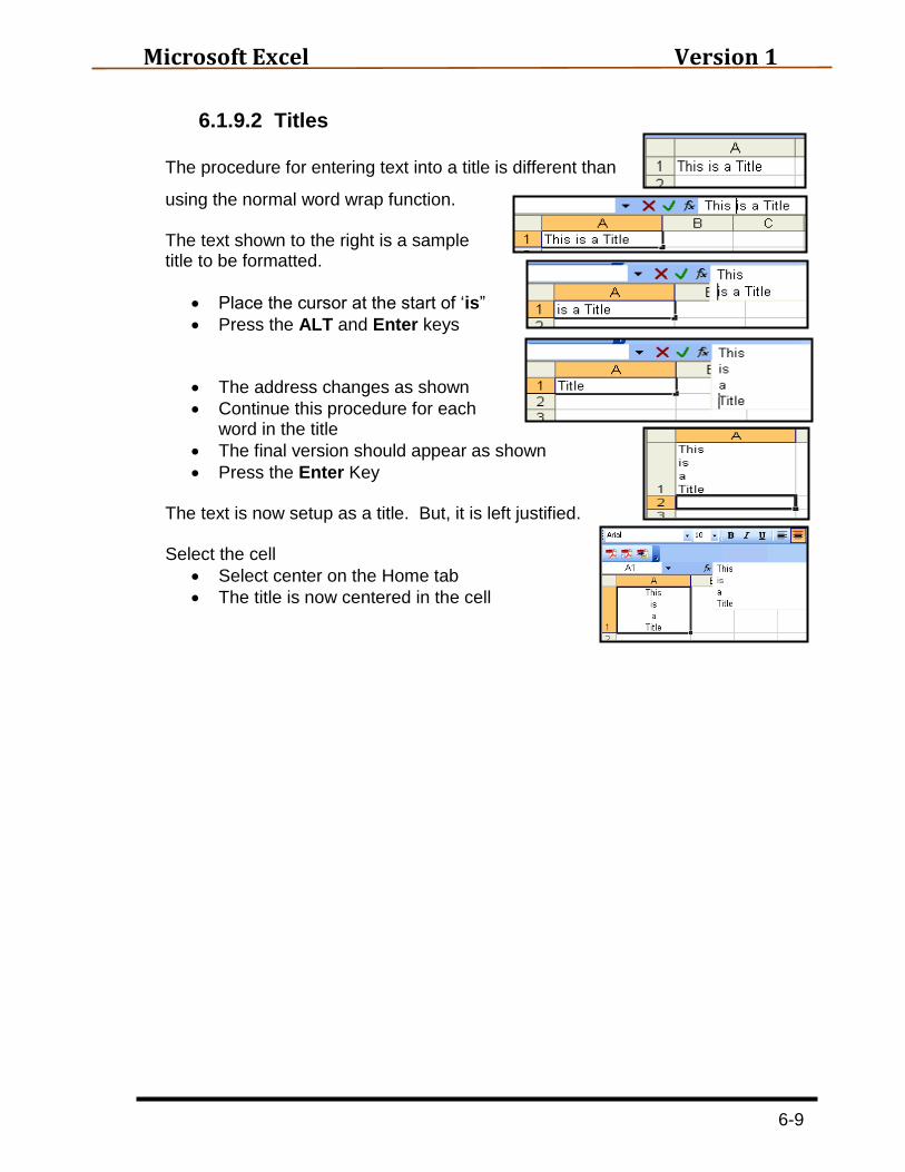
The procedure for entering text into a title is different than

using the normal word wrap function. The text shown to the right is a sample title to be formatted.

Place the cursor at the start of ‘is”

Press the ALT and Enter keys

The address changes as shown

Continue this procedure for each word in the title

The final version should appear as shown

Press the Enter Key The text is now setup as a title. But, it is left justified. Select the cell

Select center on the Home tab

The title is now centered in the cell


6-10

6.2 Conditional Formatting

The format of a cell can be changed based on the number meeting certain conditions. This type of formatting is called Conditional Formatting. Conditional formatting can be applied to a cell, range of cells or the entire workbook. The most common use is to highlight a cell or range of cells if the condition warrants it. The background color of a cell or the color of the font can be changed if the cell value is within a certain range. To open the activate Conditional Formatting window, highlight cells affected, click Home tab / Conditional Formatting.

In this example, any number greater than 40000 is to be flagged. As shown, a live preview shows the results. The Format condition was to make the cell a light red.

The result is that cell in column D are shaded red because the value exceeds 40,000.


7-1

7 6BCharts

7.1 Insert a Chart

With Excel’s Insert tab, creating graphs is an easy point-and-click process. It guides you through each of the steps necessary to create a professional-looking chart. After you select the data you want to chart, click the chart type icon on the Insert tab, Charts group. A chart of the selected data appears on the screen along with the Charts Tools tab.

7.1.1 Select Data

Highlight the data to be graphed. Select the numeric data and associated row and column labels. Excel uses the labels in the chart.

For example, in the figure, select cells A4 through E8 to graph the monthly figures for each region.

If the data is not contiguous, use Excel’s multiple selection technique; select the first range of data, hold down the Ctrl key then select the second range of data.

Then, click the Insert tab and select the appropriate chart type for the data.


7-2

7.1.2 Charts Group

7.1.2.1 Chart Type

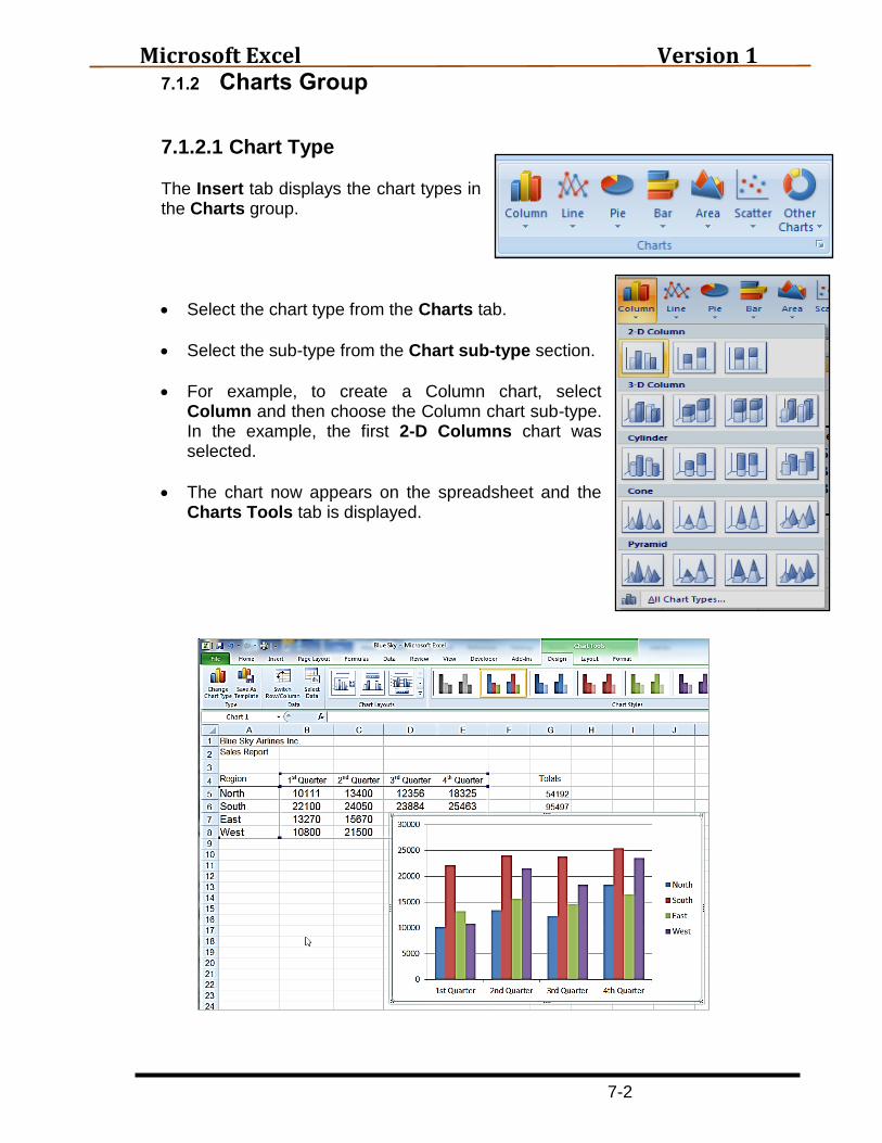
The Insert tab displays the chart types in the Charts group.

Select the chart type from the Charts tab.

Select the sub-type from the Chart sub-type section.

For example, to create a Column chart, select Column and then choose the Column chart sub-type. In the example, the first 2-D Columns chart was selected.

The chart now appears on the spreadsheet and the Charts Tools tab is displayed.


7-3

7.1.2.2 Chart Terms

7.1.2.3 Chart Tools

7.1.2.3.1 Design Tab

The Design tab provides a number of features that can be used to set/modify the design of a chart. They range from changing the chart type to moving its location.

Switch Row/Column – changes the orientation of the chart by reversing the row – column arrangement. The entries that were shown in the spreadsheet as rows are transposed to be in columns instead.

Select Data – Provides ability to select the spreadsheet data to be used in the chart.


7-4

Chart Layout – Changes the overall layout of the chart. Selection of one of the options displayed in the gallery provides the text areas for titles.

Initial format Format 9 was selected.

Chart Styles – Changes the overall visual style of the chart. Another gallery with a wide choice of styles.

Location – Moves the chart to another worksheet or as a tab in the workbook.


7-5

7.1.2.3.2 Layout Tab

The layout tab provides the ability to add features to the chart such as Data Labels, Data Tables, Gridlines, and Backgrounds. Several of these options are automatically included when the layout is selected in the Design tab.

7.1.2.3.3 Format Tab

The Format tab provides the ability to change the format of each of the parts of the chart from the Chart Area to individual data series.

7.2 Edit An Excel chart is a worksheet object. Like other worksheet objects, it can be modified by changing its size, moving or deleting it.

7.2.1 Changing the Chart Size

To change the size of a chart,

Click on the chart to select it. Small selection boxes appear on each corner of the chart.

Drag one of the selection handles to make the chart larger or smaller.

7.2.2 Moving

To move the chart, press the mouse on the border of the chart and drag the mouse as described in the previous section.

7.2.3 Deleting

Select the chart and press Delete or Backspace to delete it.


7-6

7.2.4 Adding Data

7.2.4.1 Change Data

The information displayed in a chart is directly linked to the data in the worksheet. As data entries with the spreadsheet change, the corresponding chart information also changes.

7.2.4.2 New Data

In the sample data, another series of values for International is to be added.

Click on the chart to open the Charts Tools tab.

On the Design tab, click on Select Data.

The Select Data Source window will open.

Select the red arrow in Chart data range line.

The window changes, permitting the user to select the new data range.

The Select Data Source window now reflects the addition of another data series.

The chart now contains the additional data series.


8-1

8 7BWorking With Excel

8.1 Spell Checking

Excel provides access to the same Spell Checker that is available throughout the Microsoft Office programs. It can be accessed from Review tab or from the Quick Access tool bar.

To spell check a spreadsheet, select cell A1 and then click on the spell checker. For this example, the word Pay was mistyped to Psy. The Spell Checker identified the error and displayed the window shown at the right. It provides a list of suggested corrections. If none of the selections are correct, just type the correct spelling and click change. If the spelling is not wrong and is as desired, click either Ignore Once or Ignore All as needed. When the checker has completed, the message at the right will be displayed.

8.2 Changing Sheet Names

At the bottom of each workbook are tabs that contain the name of each spreadsheet. Excel automatically names them Sheet 1, Sheet 2, etc. By clicking on the tab for Sheet 2, Sheet 2 is immediately displayed. To return to sheet 1, click the appropriate tab.

To change the sheet name, double click the sheet tab.

Type the new name and press enter. The new name is now on the worksheet tab.


8-2

8.3 Move a Worksheet The sequence or order of the worksheets can be changed by using either of two methods.

Cursor o Place the cursor on the sheet to be

moved. o Hold down the left mouse button and a small ‘document symbol will

appear at the cursor. Also, a small black arrow will appear to the left and above the tab.

o Holding the left button down, slide the cursor to the right or left as required. The black arrow will move in the same direction.

o When the new position for the worksheet is reached, release the left button.

Window o Right click on the tab or worksheet to be moved. o The window opens, click the Move or Copy

selection. o The Move or Copy window will open o The worksheet will be placed before the worksheet

selected in the window. In the example, PBCSD would be placed before Sheet 2.

This technique can also be used to copy a worksheet to a new worksheet or to a new workbook.

8.4 Copying Across Worksheets

Data and formulas can be copied across multiple worksheets. It uses the Fill Across Worksheets command. The first step is to group the worksheets. Select the first worksheet and then hold down the Shift key and select the last sheet. In the example, that is to select sheet 1 and then sheet 3.

The selected sheets are highlighted and the word [Group] appears on the title line next to the workbook name. The data typed on the active worksheet will be filled across all of the other worksheets in the group in exactly the same location on each worksheet.


8-3

8.5 Linking Files An external link is created when a cell reference is made to a different workbook. Why use them? If Principals/Department Heads are creating workbooks, the respective Chief Officer might want to produce a workbook showing data from all Areas/Schools. Linking the Areas/Schools workbooks can accomplish this task. Excel tracks the full path of a source workbook, if it is closed, by placing the full path of the source workbook in the cell reference. (Example: ='C:\WORK\[SALES.XLS]Sheet 1'!$B$1 Updating a source workbook:

a. Excel will automatically update any workbook containing links when the file is opened. A dialogue box will open, asking if the workbook should be updated. This message option can be switched off, and the workbook will be updated automatically whenever the file is opened.

b. The update will occur even if the source workbook is closed. c. Manual updates can be used to stop files that otherwise would become too

large for the program to handle

8.6 Freeze Panes

When large worksheets are being displayed, it may become difficult to remember row or column titles that have scrolled off the screen. Excel provides the ability to freeze selected rows and/or columns on the screen while scrolling across the length or breath of a large worksheet. On the View tab, in the Window group, click Freeze Panes.

Freeze Panes will freeze all rows and columns above and to the left of the active cell. To unfreeze the cells, again select the Window menu. The Freeze panes words will now say Unfreeze Panes. Click on this phrase.

In this example, cell A3 was selected as the active cell. When Freeze Panes is selected, rows 1 and 2 are frozen and a heavy line is drawn between rows 2 and 3 to indicate they are frozen.


8-4

In this example, cell B3 was selected. Rows 1 and 2 as well as column A were frozen.

The spreadsheet was scrolled to the left and down. As can be seen, rows 1 and 2 as well as column A stayed constant. The rows were down to 34 and the columns were moved left to AN.

8.7 Filtering Data Large spreadsheets frequently contain large lists of data that overwhelm the user. The Filter tool permits the ability to look at data that has a selected value in a cell or a custom range of values. This section is to provide an overview of the Filter procedures. It is not an in-depth explanation.

On the Data tab, in the Sort & Filter group, click Filter. Window control buttons open on each of the included columns as shown to the left.

Click on one of the control buttons, and another window opens. This window identifies the items in column, the ability to sort and the ability to create a custom filter.

A second filter capability is available. Selection of the Custom Filter option produces this window. It can be used to customize the filter and to work with a criteria range.


8-5

8.8 Sorting 8.8.1 86BSimple Sorts

To quickly sort data in your worksheet, even if the data doesn’t appear in a table, first click a single cell in the column by which you want to sort, and then click the Sort & Filter button on the Home ribbon. Select the ascending sort (which sorts data alphabetically from A to Z or from 0 to 9, as opposed to a descending sort, which sorts from Z to A, or from 9 to 0). Excel selects all the data in your selected column as well as the columns of data that touch that column so that all your rows of data sort together properly.

8.8.2 87BSorting by Multiple Columns

The Sort dialog box lets you sort multiple columns as one time. To open the Sort dialog box, display your Data ribbon and click Sort to open the Sort dialog box. Excel 2010 now lets you specify up to 64 columns for your sort order, using ascending or descending order for each one.


9-1

9 8BPrinting

9.1 Worksheet After creating a workbook and saving it to a folder, it may be necessary to print it on paper. That is, to create a hardcopy of the spreadsheet. Click the File tab, and then click on Print .

Select the Print button to print the selected spreadsheet/workbook.


9-2

9.1.1 88BPage Setup.

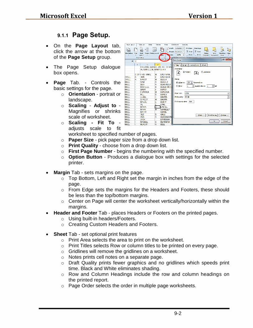
On the Page Layout tab, click the arrow at the bottom of the Page Setup group.

The Page Setup dialogue box opens.

Page Tab. - Controls the basic settings for the page.

o Orientation - portrait or landscape.

o Scaling - Adjust to - Magnifies or shrinks scale of worksheet.

o Scaling - Fit To - adjusts scale to fit worksheet to specified number of pages.

o Paper Size - pick paper size from a drop down list. o Print Quality - choose from a drop down list. o First Page Number - begins the numbering with the specified number. o Option Button - Produces a dialogue box with settings for the selected

printer.

Margin Tab - sets margins on the page. o Top Bottom, Left and Right set the margin in inches from the edge of the

page. o From Edge sets the margins for the Headers and Footers, these should

be less than the top/bottom margins. o Center on Page will center the worksheet vertically/horizontally within the

margins.

Header and Footer Tab - places Headers or Footers on the printed pages. o Using built-in headers/Footers. o Creating Custom Headers and Footers.

Sheet Tab - set optional print features o Print Area selects the area to print on the worksheet. o Print Titles selects Row or column titles to be printed on every page. o Gridlines will remove the gridlines on a worksheet. o Notes prints cell notes on a separate page. o Draft Quality prints fewer graphics and no gridlines which speeds print

time. Black and White eliminates shading. o Row and Column Headings include the row and column headings on

the printed report. o Page Order selects the order in multiple page worksheets.


9-3

9.1.2 89BManual Page Breaks Excel will place automatic page breaks in the worksheets. These are visible in Print Preview. Manual Page Breaks are placed on the worksheet using Insert on the Menu bar.

Selecting a cell will put the page break above and to left of that column or cell.

Then click your Page Layout ribbon’s Breaks button, and choose Insert Page Break.

To remove the page break, choose the Break’s Remove Page Break option.

9.2 WorkBook

To print a selected range in worksheet, o Select the area to be printed. o On the print dialogue box, in the "Print

what" area, choose Selection.

To print specific pages of a workbook or worksheet, o Select Pages From at the bottom of the

print dialogue box. o Type in the page numbers.

To print a selected range in worksheet, o Select the area to be printed. o On the print dialogue box, in the "Print what" area, choose Selection.

To print specific pages of a workbook or worksheet, o Select Pages From at the bottom of the print dialogue box. o Type in the page numbers.


10-1

10 10BOnline Resources Microsoft offers a number of sites that can be accessed to assist with understanding Office 2010. The web page is 2TUhttp://office.microsoft.com/en-us/trainingU2T. Notice that there is no www in the URL This page provides an agenda of the training courses, presentations and demos that are available for Office 2010 as well as Office 2007 and Office 2003.

10.1 48BTraining Training Courses for Office 2010 can be accessed from this screen.

http://office.microsoft.com/en-us/training


10-2

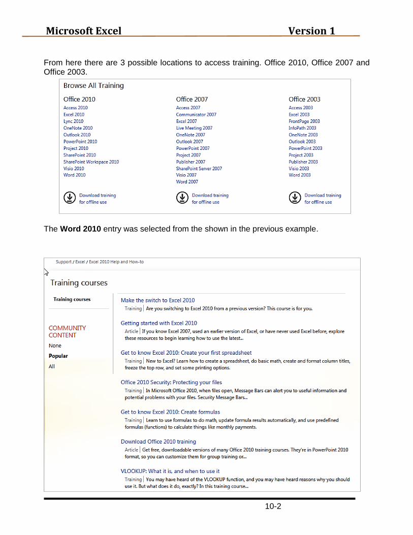
From here there are 3 possible locations to access training. Office 2010, Office 2007 and Office 2003.

The Word 2010 entry was selected from the shown in the previous example.


10-3

10.2 Excel Help System It is very easy to be overwhelmed by all of the features in Excel. Many times there will be a procedure you would like to accomplish, but just are not sure how to do it. Excel provides a help system that can provide multiple answers to most questions asked.

Click on the Help button on the Ribbon.

The result will be access to the help menu.

10.3 Training Manual This manual is maintained on the District’s Web page. It is updated periodically to add new features as they are identified by the students and by the trainers. The online version of this training manual can be accessed by going to http://www.palmbeachschools.org/it/techtraining.asp. This link opens the Technical Training page. This page contains the training schedules and the training manuals used for Office 2003, 2007 and 2010.

Select the desired manual and click on it. The manual will open as a PDF that can be viewed or printed.

http://www.palmbeachschools.org/it/techtraining.asp


11-1

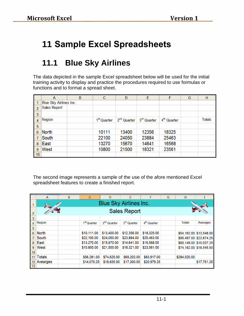
11 11BSample Excel Spreadsheets

11.1 Blue Sky Airlines The data depicted in the sample Excel spreadsheet below will be used for the initial training activity to display and practice the procedures required to use formulas or functions and to format a spread sheet.

The second image represents a sample of the use of the afore mentioned Excel spreadsheet features to create a finished report.


11-2

11.2 Amortization Schedule An amortization schedule is included to depicts examples of a wide range of excel functions and spreadsheet cell management. The following tables show the data to be entered into the spreadsheet.

11.2.1 90BTable 1

Note: Cell identifies the cell address on the spreadsheet to be used. Entry identifies the information to be entered into the cell.

Cell Entry

B2 Loan Calculator

B5 Interest Rate

C5 Term (months)

D5 Loan Amount

G5 Monthly Payment

B6 10.0% {be sure to type the % sign}

C6 24

D6 2000

G6 =PMT(B6/12,C6,-D6)

Entry of the information shown in Table 1 would produce the following spreadsheet.


11-3

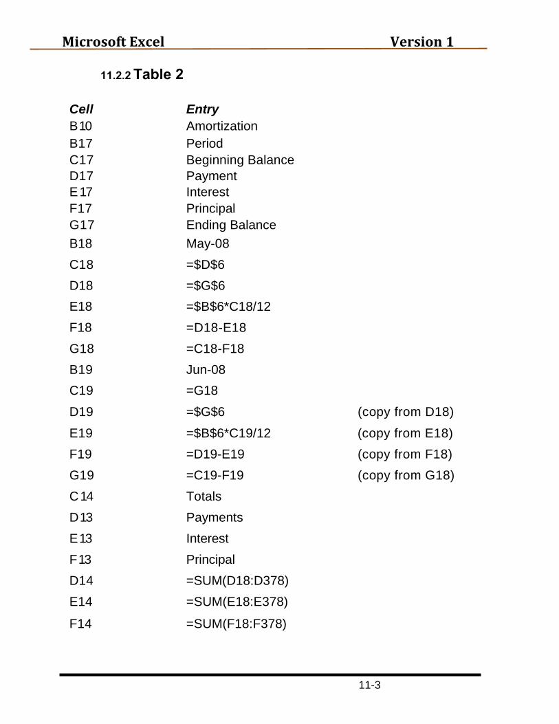
11.2.2 91BTable 2

Cell Entry

B 10 Amortization

B17 Period

C17 Beginning Balance

D17 Payment

E 17 Interest

F17 Principal

G17 Ending Balance

B18 May-08

C18 =$D$6

D18 =$G$6

E18 =$B$6*C18/12

F18 =D18-E18

G18 =C18-F18

B19 Jun-08

C19 =G18

D19 =$G$6 (copy from D18)

E19 =$B$6*C19/12 (copy from E18)

F19 =D19-E19 (copy from F18)

G19 =C19-F19 (copy from G18)

C 14 Totals

D 13 Payments

E 13 Interest

F 13 Principal

D14 =SUM(D18:D378)

E14 =SUM(E18:E378)

F14 =SUM(F18:F378)


11-4

Entry of the additional information shown in Table 2 would produce the following spreadsheet. It includes the data from Table 1 and Table 2.

The final step is to generate the additional rows of data that would be needed to display the ending balance of $0.00.


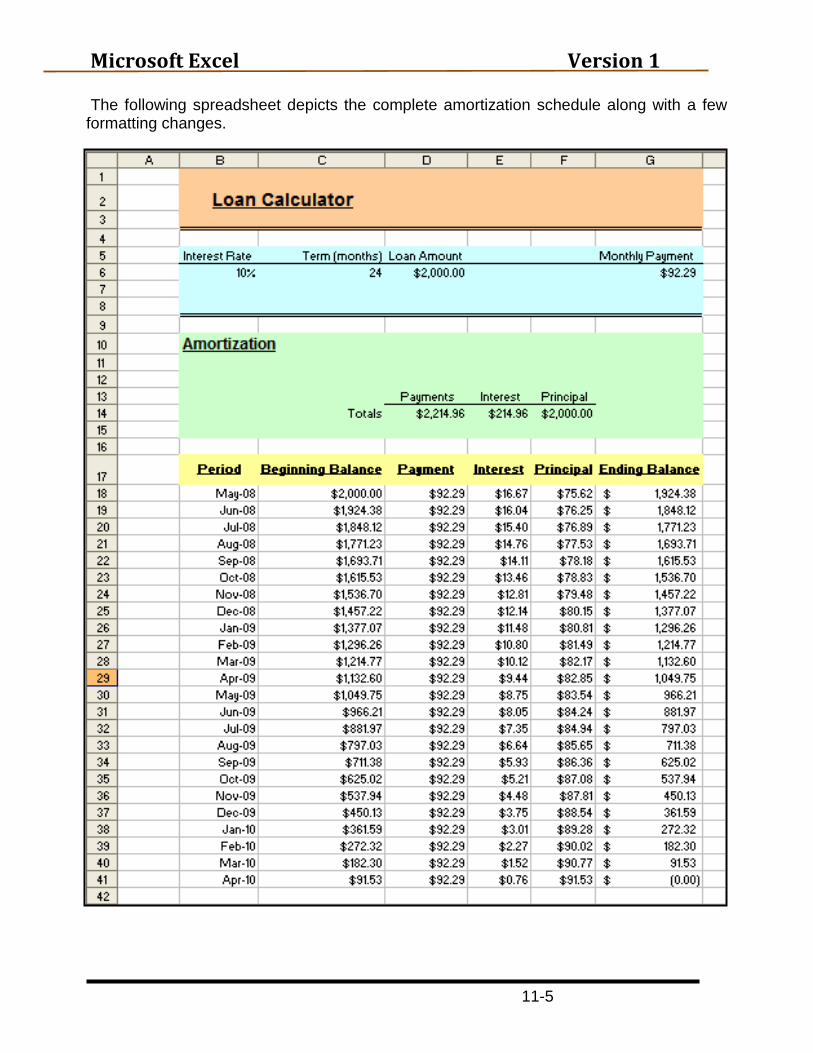
11-5

The following spreadsheet depicts the complete amortization schedule along with a few formatting changes.