a guided tour of mathematical methods
TRANSCRIPT

A GUIDED TOUR OF MATHEMATICAL METHODSFor the Physical Sciences
Second Edition
Mathematical methods are essential tools for all physical scientists. This secondedition of A Guided Tour of Mathematical Methods provides a comprehensive tourof the mathematical knowledge and techniques that are needed by students in thisarea. In contrast to more traditional textbooks, all the material is presented in theform of problems. Within these problems the basic mathematical theory and itsphysical applications are well integrated. The mathematical insights that the stu-dent acquires are therefore driven by their physical insight. Topics that are coveredinclude vector calculus, linear algebra, Fourier analysis, scale analysis, complexintegration, Green’s functions, normal modes, tensor calculus, and perturbationtheory. The second edition contains new chapters on dimensional analysis, varia-tional calculus, and the asymptotic evaluation of integrals. This book can be usedby undergraduates and lower-level graduate students in the physical sciences. It canserve as a stand-alone text, or as a source of problems and examples to complementother textbooks.
Roel Snieder holds the Keck Foundation Endowed Chair of Basic ExplorationScience at the Colorado School of Mines. He received his Masters degree in Geo-physical Fluid Dynamics from Princeton University in 1984 and in 1987 a Ph.D.in seismology from Utrecht University. In 1993 he was appointed as professor ofseismology at Utrecht University, where from 1997 to 2000 he served as Dean ofthe Faculty of Earth Sciences. In 1997 he was a visiting professor at the Centerfor Wave Phenomena at the Colorado School of Mines. His research focuses onwave propagation and inverse problems. He has served on the editorial boards ofGeophysical Journal International, Inverse Problems, and Reviews of Geophysics.In 2000 he was elected as Fellow of the American Geophysical Union for importantcontributions to geophysical inverse theory, seisic tomography, and the theory ofsurface waves.

A GUIDED TOUR OF MATHEMATICALMETHODS
For the Physical Sciences
Second Edition
ROEL SNIEDERDepartment of Geophysics and Center for Wave Phenomena, Colorado School of Mines

CAMBRIDGE UNIVERSITY PRESS
Cambridge, New York, Melbourne, Madrid, Cape Town, Singapore, São Paulo, Delhi
Cambridge University Press
The Edinburgh Building, Cambridge CB2 8RU, UK
Published in the United States of America by Cambridge University Press, New York
www.cambridge.org
Information on this title: www.cambridge.org/9780521542616
© R. Snieder 2004
This publication is in copyright. Subject to statutory exception
and to the provisions of relevant collective licensing agreements,
no reproduction of any part may take place without the written
permission of Cambridge University Press.
First published 2004
Reprinted 2006
This digitally printed version 2009
A catalogue record for this publication is available from the British Library
Library of Congress Cataloguing in Publication data
Snieder, Roel, 1958–
A guided tour of mathematical methods for the physical sciences/Roel Snieder – 2nd ed.
p. cm
Includes bibliographical references and index.
ISBN 0 521 83492 9 (hardback)
1. Mathematical analysis. 2. Physical sciences – Mathematics. 3. Mathematical physics. I. Title.
QA300.S794 2004
515–dc22 2004040783
ISBN 978-0-521-83492-6 hardback
ISBN 978-0-521-54261-6 paperback
Cambridge University Press has no responsibility for the persistence or accuracy of URLs
for external or third-party Internet websites referred to in this publication, and does not
guarantee that any content on such websites is, or will remain, accurate or appropriate.

To Idske, Hylke, Hidde and Julia


Contents
Preface to Second Edition page xiiiAcknowledgements xiv
1 Introduction 12 Dimensional analysis 32.1 Two rules for physical analysis 32.2 A trick for finding mistakes 62.3 Buckingham pi theorem 72.4 Lift of a wing 112.5 Scaling relations 122.6 Dependence of pipe flow on the radius of the pipe 133 Power series 163.1 Taylor series 163.2 Growth of the Earth by cosmic dust 223.3 Bouncing ball 243.4 Reflection and transmission by a stack of layers 274 Spherical and cylindrical coordinates 314.1 Introducing spherical coordinates 314.2 Changing coordinate systems 354.3 Acceleration in spherical coordinates 374.4 Volume integration in spherical coordinates 404.5 Cylindrical coordinates 435 Gradient 465.1 Properties of the gradient vector 465.2 Pressure force 505.3 Differentiation and integration 535.4 Newton’s law from energy conservation 555.5 Total and partial time derivatives 575.6 Gradient in spherical coordinates 61
vii
viii Contents
6 Divergence of a vector field 646.1 Flux of a vector field 646.2 Introduction of the divergence 666.3 Sources and sinks 696.4 Divergence in cylindrical coordinates 716.5 Is life possible in a five-dimensional world? 737 Curl of a vector field 787.1 Introduction of the curl 787.2 What is the curl of the vector field? 807.3 First source of vorticity: rigid rotation 817.4 Second source of vorticity: shear 837.5 Magnetic field induced by a straight current 857.6 Spherical coordinates and cylindrical coordinates 868 Theorem of Gauss 888.1 Statement of Gauss’s law 888.2 Gravitational field of a spherically symmetric mass 898.3 Representation theorem for acoustic waves 918.4 Flowing probability 939 Theorem of Stokes 979.1 Statement of Stokes’s law 979.2 Stokes’s theorem from the theorem of Gauss 1009.3 Magnetic field of a current in a straight wire 1029.4 Magnetic induction and Lenz’s law 1039.5 Aharonov–Bohm effect 1049.6 Wingtips vortices 10810 Laplacian 11310.1 Curvature of a function 11310.2 Shortest distance between two points 11710.3 Shape of a soap film 12010.4 Sources of curvature 12410.5 Instability of matter 12610.6 Where does lightning start? 12810.7 Laplacian in spherical and cylindrical coordinates 12910.8 Averaging integrals for harmonic functions 13011 Conservation laws 13311.1 General form of conservation laws 13311.2 Continuity equation 13511.3 Conservation of momentum and energy 13611.4 Heat equation 14011.5 Explosion of a nuclear bomb 145
Contents ix
11.6 Viscosity and the Navier–Stokes equation 14711.7 Quantum mechanics and hydrodynamics 15012 Scale analysis 15312.1 Vortex in a bathtub 15412.2 Three ways to estimate a derivative 15612.3 Advective terms in the equation of motion 15912.4 Geometric ray theory 16212.5 Is the Earth’s mantle convecting? 16712.6 Making an equation dimensionless 16913 Linear algebra 17313.1 Projections and the completeness relation 17313.2 Projection on vectors that are not orthogonal 17713.3 Coriolis force and centrifugal force 17913.4 Eigenvalue decomposition of a square matrix 18413.5 Computing a function of a matrix 18713.6 Normal modes of a vibrating system 18913.7 Singular value decomposition 19213.8 Householder transformation 19714 Dirac delta function 20214.1 Introduction of the delta function 20214.2 Properties of the delta function 20614.3 Delta function of a function 20814.4 Delta function in more dimensions 21014.5 Delta function on the sphere 21014.6 Self energy of the electron 21215 Fourier analysis 21715.1 Real Fourier series on a finite interval 21715.2 Complex Fourier series on a finite interval 22115.3 Fourier transform on an infinite interval 22315.4 Fourier transform and the delta function 22415.5 Changing the sign and scale factor 22515.6 Convolution and correlation of two signals 22815.7 Linear filters and the convolution theorem 23115.8 Dereverberation filter 23415.9 Design of frequency filters 23815.10 Linear filters and linear algebra 24016 Analytic functions 24516.1 Theorem of Cauchy–Riemann 24516.2 Electric potential 24916.3 Fluid flow and analytic functions 251

x Contents
17 Complex integration 25417.1 Nonanalytic functions 25417.2 Residue theorem 25517.3 Solving integrals without knowing the primitive function 25917.4 Response of a particle in syrup 26218 Green’s functions: principles 26718.1 Girl on a swing 26718.2 You have seen Green’s functions before! 27218.3 Green’s functions as impulse response 27318.4 Green’s functions for a general problem 27618.5 Radiogenic heating and the Earth’s temperature 27918.6 Nonlinear systems and the Green’s functions 28419 Green’s functions: examples 28819.1 Heat equation in N dimensions 28819.2 Schrodinger equation with an impulsive source 29219.3 Helmholtz equation in one, two, and three dimensions 29619.4 Wave equation in one, two, and three dimensions 30219.5 If I can hear you, you can hear me 30820 Normal modes 31120.1 Normal modes of a string 31220.2 Normal modes of a drum 31420.3 Normal modes of a sphere 31720.4 Normal modes of orthogonality relations 32320.5 Bessel functions behave as decaying cosines 32720.6 Legendre functions behave as decaying cosines 33020.7 Normal modes and the Green’s function 33420.8 Guided waves in a low-velocity channel 34020.9 Leaky modes 34420.10 Radiation damping 34821 Potential theory 35321.1 Green’s function of the gravitational potential 35421.2 Upward continuation in a flat geometry 35621.3 Upward continuation in a flat geometry in three dimensions 35921.4 Gravity field of the Earth 36121.5 Dipoles, quadrupoles, and general relativity 36521.6 Multipole expansion 36921.7 Quadrupole field of the Earth 37421.8 Fifth force 37722 Cartesian tensors 37922.1 Coordinate transforms 379

Contents xi
22.2 Unitary matrices 38222.3 Shear or dilatation? 38522.4 Summation convention 38922.5 Matrices and coordinate transforms 39122.6 Definition of a tensor 39322.7 Not every vector is a tensor 39622.8 Products of tensors 39822.9 Deformation and rotation again 40122.10 Stress tensor 40322.11 Why pressure in a fluid is isotropic 40622.12 Special relativity 40823 Perturbation theory 41223.1 Regular perturbation theory 41323.2 Born approximation 41723.3 Linear travel time tomography 42123.4 Limits on perturbation theory 42423.5 WKB approximation 42723.6 Need for consistency 43123.7 Singular perturbation theory 43324 Asymptotic evaluation of integrals 43724.1 Simplest tricks 43724.2 What does n! have to do with e and
√π ? 441
24.3 Method of steepest descent 44524.4 Group velocity and the method of stationary phase 45024.5 Asymptotic behavior of the Bessel function J0(x) 45324.6 Image source 45625 Variational calculus 46125.1 Designing a can 46125.2 Why are cans round? 46325.3 Shortest distance between two points 46525.4 The great-circle 46825.5 Euler–Lagrange equation 47225.6 Lagrangian formulation of classical mechanics 47625.7 Rays are curves of stationary travel time 47825.8 Lagrange multipliers 48125.9 Designing a can with an optimal shape 48525.10 The chain line 48726 Epilogue, on power and knowledge 492
References 494Index 500


Preface to Second Edition
The updates and changes from the earlier version of the book have to a large extentbeen driven by the comments of readers and reviewers. The second edition has beenextendedwithChapters 2, 24, and25 that cover dimensional analysis, the asymptoticevaluation of integrals, and variational calculus, respectively. In a few places, newmaterial has been inserted, such as Section 19.5 that covers the reciprocity of wavepropagation. A number of teachers and students remarked that the level of difficultyof the problems in the first edition was highly variable. The problems in the secondedition contain more hints and advice to make these problems more tractable.
xiii
Acknowledgements
This book resulted from two courses on mathematical physics that were taught atUtrecht University. The remarks, corrections, and the encouragement of a largenumber of students have been very important in its development. It is impossi-ble to thank all the students, but I especially want to thank the feedback fromJojanneke van den Berg, Jehudi Blom, Sterre Dortland, Thomas Geenen, Wiebevan Driel, Luuk van Gerven, Noor Hogeweg, and Frederiek Siegenbeek. In theirrole as teaching assistants,DirkKraaipoel and Jesper Spetzler have helped greatly inimproving this book. Huub Douma has spent numerous hours at sea correcting ear-lier drafts. A number of colleagues have helpedme verymuchwith their comments;I especiallywant tomention FreemanGilbert, AlexanderKaufman,AntoineKhater,Ken Larner, and Jeannot Trampert. Many of the figures were drafted by BarbaraMcLenon, who I thank for her support. The help of Joop Hoofd, EverhardMuyzert,and John Stockwell, who patiently coped with my computer illiteracy, allowed meto prepare this book electronically. TerryYoung greatly helpedme tomake the indexof the second edition. The support and advice of Adam Black, Eoin O’Sullivan,Jayne Aldhouse, Maureen Storey, Joseph Bottrill, Keith Westmoreland and SimonCapelin of Cambridge University Press has been very helpful and stimulatingduring the preparation of this work. Lastly, I want to thank everybody who helpedme in numerous ways to make writing this book a joy.
xiv
1
Introduction
The topic of this book is the application of mathematics to physical problems.Mathematics and physics are often taught separately. Despite the fact that educationin physics relies on mathematics, it turns out that students consider mathematicsto be disjoint from physics. Although this point of view may strictly be correct,it reflects an erroneous opinion when it concerns an education in the sciences.The reason for this is that mathematics is the only language at our disposal forquantifying physical processes. One cannot learn a language by just studying atextbook. In order to truly learn how to use a language one has to go abroad and startusing that language. By the same token one cannot learn how to use mathematics inthe physical sciences by just studying textbooks or attending lectures; the only wayto achieve this is to venture into the unknown and apply mathematics to physicalproblems.
It is the goal of this book to do exactly that; problems are presented in order toapply mathematical techniques and knowledge to physical concepts. These exam-ples are not presented as well-developed theory. Instead, they are presented as anumber of problems that elucidate the issues that are at stake. In this sense this bookoffers a guided tour: material for learning is presented but true learning will onlytake place by active exploration. In this process, the interplay of mathematics andphysics is essential; mathematics is the natural language for physics while physicalinsight allows for a better understanding of the mathematics that is presented.
How can you use this book most efficiently?
Since this book is written as a set of problems you may frequently want to consultother material as well to refresh or deepen your understanding of material. In manyplaces we refer to the book of Boas [19]. In addition, the books of Butkov [24],Riley et al. [87] and Arfken [5] on mathematical physics are excellent.
1
2 Introduction
In addition to books, colleagues in either the same field or other fields can be agreat source of knowledge and understanding. Therefore, do not hesitate to worktogether with others on these problems if you are in the fortunate position to do so.This may not only make the work more enjoyable, it may also help you in getting“unstuck” at difficult moments and the different viewpoints of others may help todeepen yours.
For who is this book written?
This book is set up with the goal of obtaining a good working knowledge of math-ematical physics that is needed for students in physics or geophysics. A certainbasic knowledge of calculus and linear algebra is required to digest the materialpresented here. For this reason, this book is meant for upper-level undergraduatestudents or lower-level graduate students, depending on the background and skillof the student. In addition, teachers can use this book as a source of examples andillustrations to enrich their courses.
This book is evolving
This book will be improved regularly by adding newmaterial, correcting errors andmaking the text clearer. The feedback of both teachers and students who use thismaterial is vital in improving this text, please send your remarks to:
Roel Snieder
Dept of Geophysics
Colorado School of MinesGolden CO 80401
USA
telephone: +1-303-273.3456fax: +1-303-273.3478
email: [email protected]
Errata can be found at the following website: www.mines.edu/ rsnieder/Errata.html.
2
Dimensional analysis
The material of this chapter is usually not covered in a book on mathematics.The field of mathematics deals with numbers and numerical relationships. It doesnot matter what these numbers are; they may account for physical properties ofa system, but they may equally well be numbers that are not related to anythingphysical. Consider the expression g = d f/dt . From a mathematical point of viewthese functions can be anything, as long as g is the derivative of f . The situation isdifferent in physics. When f (t) is the position of a particle, and t denotes time, theng(t) is a velocity. This relation fixes the physical dimension of g(t). In mathematicalphysics, the physical dimension of variables imposes constraints on the relationbetween these variables. In this chapter we explore these constraints. In Section 2.2we show that this provides a powerful technique for spotting errors in equations. Inthe remainder of this chapter we show how the physical dimensions of the variablesthat govern a problem can be used to find physical laws. Surprisingly, while mostengineers learn about dimensional analysis, this topic is not covered explicitly inmany science curricula.
2.1 Two rules for physical dimensions
In physics every physical parameter is associated with a physical dimension. Thevalue of each parameter is measured with a certain physical unit. For example,when I measure how long a table is, the result of this measurement has dimension“length”. This length is measured in a certain unit, that may be meters, inches,furlongs, or whatever length unit I prefer to use. The result of this measurementcan be written as
l = 3 m. (2.1)
3

4 Dimensional analysis
The variable l has the physical dimension of length, in this chapter we write this as
l ∼ [L]. (2.2)
The square brackets are used in this chapter to indicate a physical dimension. Thecapital letter L denotes length, T denotes time, and M denotes mass. Other physicaldimensions include electric charge and temperature. When dealing with physicaldimensions two rules are useful. The first rule is:
Rule 1 When two variables are added, subtracted, or set equal to each other, theymust have the same physical dimension.
In order to see the logic of this rule we consider the following example. Supposewe have an object with a length of 1 meter and a time interval of one second. Thismeans that
l = 1 m,
t = 1 s.(2.3)
Since both variables have the same numerical value, we might be tempted to declarethat
l = t. (2.4)
It is, however, important to realize that the physical units that we use are arbitrary.Suppose, for example, that we had measured the length in feet rather than meters.In that case the measurements (2.3) would be given by
l = 3 ft,t = 1 s.
(2.5)
Now the numerical value of the same length measurement is different! Since thechoice of the physical units is arbitrary, we can scale the relation between variablesof different physical dimensions in an arbitrary way. For this reason these variablescannot be equal to each other. This implies that they cannot be added or subtractedeither.
The first rule implies the following rule.
Rule 2 Mathematical functions can act on dimensionless numbers only.
To see this, let us consider as an example the function f (ξ ) = eξ . Using a Taylorexpansion, this function can be written as:
f (ξ ) = 1 + ξ + 1
2ξ 2 + · · · (2.6)

2.1 Two rules for physical analysis 5
According to rule 1 the different terms in this expression must have the samephysical dimension. The first term (the number 1) is dimensionless, hence all theother terms in the series must be dimensionless. This means that ξ must be adimensionless number as well. This argument can be used for any function f (ξ )whose Taylor expansion contains different powers of ξ . Note that the argumentwould not hold for a function such as f (ξ ) = ξ 2 that contains only one power of ξ .
To please the purists, rule 2 could easily be reformulated to exclude these specialcases.
These rules have several applications in mathematical physics. Suppose we wantto find the physical dimension of a force, as expressed in the basic dimensions mass,length, and time. The only thing we need to do is take one equation that contains aforce. In this case Newton’s law F = ma comes to mind. The mass m has physicaldimension [M], while the acceleration has dimension [L/T 2]. Rule 1 implies thatforce has the physical dimension [M L/T 2].
Problem a The force F in a linear spring is related to the extension x of thespring by the relation F = −kx . Show that the spring constant k has dimension[M/T 2].
Problem b The angular momentum L of a particle with momentum p at positionr is given by
L = r × p, (2.7)
where × denotes the cross-product of two vectors. Show that angular momen-tum has the dimension [M L2/T ].
Problem c A plane wave is given by the expression
u(r, t) = ei(k·r−ωt), (2.8)
where r is the position vector and t denotes time. Show that k ∼ [L−1] andω ∼ [T −1].
In quantum mechanics the behavior of a particle is characterized by a waveequation, that is called the Schrodinger equation. In one space dimension thisequation is given by
ih∂ψ
∂t= − h2
2m
∂2ψ
∂x2+ V (x)ψ, (2.9)
where x denotes the position, t denotes the time, m the mass of the particle, andV (x) the potential energy of the particle. At this point it is not clear what the wave

6 Dimensional analysis
function ψ(x, t) is, and how this equation should be interpreted. The meaning ofthe symbol h is not yet defined. We can, however, determine the physical dimensionof h without knowing the meaning of this variable.
Problem d Compare the physical dimensions of the left-hand side of (2.9) withthe first term on the right-hand side and show that the variable h has the physi-cal dimension angular momentum. You can use problem b in showing this.
2.2 A trick for finding mistakes
The requirement that all terms in an equation have the same physical dimensionis an important tool for spotting mistakes. Cipra [26] gives many useful tips forspotting errors in his delightful book “Misteakes [sic] . . . and how to find thembefore the teacher does.” As an example of using dimensional analysis for spottingmistakes, we consider the erroneous equation
E = mc3, (2.10)
where E denotes energy, m denotes mass, and c is the speed of light. Let us first findthe physical dimension of energy. The work done by a force F over a displacementdr is given by d E = F · dr. We showed in Section 2.1 that force has the dimension[M L/T 2]. This means that energy has the dimension [M L2/T 2]. The speed of lightin the right-hand side of expression (2.10) has dimension [L/T ], which means thatthe right-hand side has physical dimension [M L3/T 3]. This is not an energy, whichhas dimension [M L2/T 2]. Therefore expression (2.10) is wrong.
Problem a Now that we have determined that expression (2.10) is incorrect wecan use the requirement that the dimensions of the different terms must matchto guess how to set it right. Show that the right-hand side must be divided bya velocity to match the dimensions.
It is not clear that the right-hand side must be divided by the speed of light to givethe correct expression E = mc2. Dimensional analysis tells us only that it must bedivided by something with the dimension of velocity. For all we know, it could bethe speed at which the average snail moves.
Problem b Is the following equation dimensionally correct?
(v · ∇v) = −∇ p. (2.11)
In this expression v is the velocity of fluid flow, p is the pressure, and ∇ isthe gradient vector (which essentially is a derivative with respect to the space
2.3 Buckingham pi theorem 7
coordinates). You can use that pressure has the dimension is force per unitarea.
Problem c Answer the same question for the expression that relates the particlevelocity v to the pressure p in an acoustic medium:
v = p
ρc(2.12)
Here ρ is the mass density and c is velocity of propagation of acoustic waves.
Problem d In quantum mechanics, the energy E of the harmonic oscillator isgiven by
En = hω2 (n + 1/2) , (2.13)
where ω is a frequency, n is a dimensionless integer, and h is Planck’s constantdivided by 2π as introduced in problem d of the previous section. Verify if thisexpression is dimensionally correct.
In general it is a good idea to carry out a dimensional analysis while workingin mathematical physics because this may help in finding the mistakes that we allmake while doing derivations. It takes a little while to become familiar with thedimensions of properties that are used most often, but this is an investment thatpays off in the long run.
2.3 Buckingham pi theorem
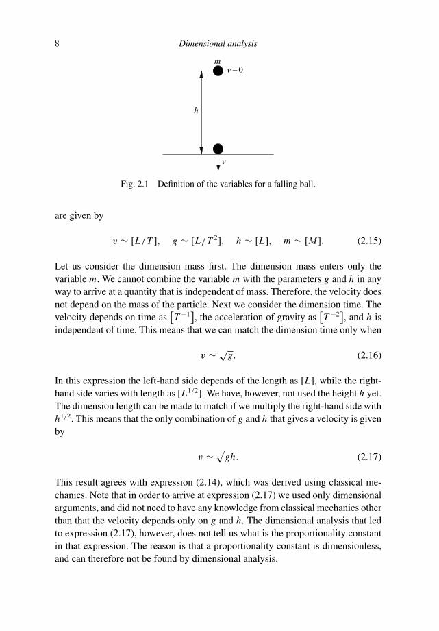
In this section we introduce the Buckingham pi theorem. This theorem can be usedto find the relation between physical parameters based on dimensional arguments.As an example, let us consider a ball shown in Figure 2.1 with mass m that isdropped from a height h. We want to find the velocity with which it strikes theground. The potential energy of the ball before it is dropped is mgh, where g isthe acceleration of gravity. This energy is converted into kinetic energy 1
2 mv2 as itstrikes the ground. Equating these quantities and solving for the velocity gives:
v =√
2gh. (2.14)
Now let us suppose we did not know about classical mechanics. In that case,dimensional analysis could be used to guess relation (2.14). We know that thevelocity is some function of the acceleration of gravity, the initial height, and themass of the particle: v = f (g, h, m). The physical dimensions of these properties
8 Dimensional analysis
v
v=0
h
m
Fig. 2.1 Definition of the variables for a falling ball.
are given by
v ∼ [L/T ], g ∼ [L/T 2], h ∼ [L], m ∼ [M]. (2.15)
Let us consider the dimension mass first. The dimension mass enters only thevariable m. We cannot combine the variable m with the parameters g and h in anyway to arrive at a quantity that is independent of mass. Therefore, the velocity doesnot depend on the mass of the particle. Next we consider the dimension time. Thevelocity depends on time as
[
T −1]
, the acceleration of gravity as[
T −2]
, and h isindependent of time. This means that we can match the dimension time only when
v ∼ √g. (2.16)
In this expression the left-hand side depends of the length as [L], while the right-hand side varies with length as [L1/2]. We have, however, not used the height h yet.The dimension length can be made to match if we multiply the right-hand side withh1/2. This means that the only combination of g and h that gives a velocity is givenby
v ∼√
gh. (2.17)
This result agrees with expression (2.14), which was derived using classical me-chanics. Note that in order to arrive at expression (2.17) we used only dimensionalarguments, and did not need to have any knowledge from classical mechanics otherthan that the velocity depends only on g and h. The dimensional analysis that ledto expression (2.17), however, does not tell us what is the proportionality constantin that expression. The reason is that a proportionality constant is dimensionless,and can therefore not be found by dimensional analysis.
2.3 Buckingham pi theorem 9
The treatment given here may appear to be cumbersome. This analysis, however,can be carried out in a systematic fashion using the Buckingham pi theorem [23]which states the following:
Buckingham pi theorem If a problem contains N variables that depend on Pphysical dimensions, then there are N − P dimensionless numbers that de-scribe the physics of the problem.
The original paper of Buckingham is very clear, but as we will see at the endof this section, this theorem is not fool-proof. Let us first apply the theorem tothe problem of the falling ball. We have four variables: v, g, h, and m, so thatN = 4. These variables depend on the physical dimensions [M], [L], and [T ],hence P = 3. According to the Buckingham pi theorem, N − P = 1 dimensionlessnumber characterizes the problem. We want to express the velocity in the otherparameters; hence we seek a dimensionless number of the form
vgαhβmγ ∼ [1], (2.18)
where the notation in the right-hand side means that it is dimensionless. Let us seekthe exponents α, β, and γ that make the left-hand side dimensionless. Inserting thedimensions of the different variables then gives the following dimensions
[
L
T
] [
Lα
T 2α
]
[
Lβ] [
Mγ] ∼ [1] . (2.19)
The left-hand side depends on length as [L1+α+β]. The left-hand side can onlybe independent of length when the exponent is equal to zero. Applying the samereasoning to each of the dimensions length, time, and mass, then gives
dimension [L]: 1 + α + β = 0,
dimension [T ]: −1 − 2α = 0,
dimension [M]: γ = 0.
(2.20)
This constitutes a system of three equations with three unknowns.
Problem a Show that the solution of this system is given by
α = β = − 1
2, γ = 0. (2.21)
Inserting these values into expression (2.18) shows that the combinationvg−1/2h−1/2 is dimensionless. This implies that
v = C√
gh, (2.22)
10 Dimensional analysis
where C is the one dimensionless number in the problem as dictated by the Buck-ingham pi theorem.
The approach taken here is systematic. In his original paper [23], Buckinghamapplied this treatment to a number of problems: the thrust provided by the screwof a ship, the energy density of the electromagnetic field, the relation between themass and radius of the electron, the radiation of an accelerated electron, and heatconduction.
There is, however, a catch that we introduce with an example. When air (or water)has a stably stratified mass–density structure, it can support oscillations where therestoring force is determined by the density gradient in the air. These oscillationsoccur with the Brunt-Vaisala frequency ωB given by [50, 82]:
ωB =√
g
θ
dθ
dz. (2.23)
In this expression, g is the acceleration of gravity, z is height, and θ is potentialtemperature (a measure of the thermal structure of the atmosphere).
Problem b Verify that this expression is dimensionally correct.
Problem c Check that this expression is also dimensionally correct when θ isreplaced by the air pressure p, or the mass density ρ.
The result of problem c indicates that the potential temperature θ can be replacedby any physical parameter, and expression (2.23) is still dimensionally correct. Thismeans that a dimensional analysis alone can never be used to prove that θ shouldbe the potential temperature. In order to show this we need to know more of thephysics of the problem.
Another limitation of the Buckingham pi theorem as formulated in its originalform is that the theorem assumes that physical parameters need to be multipliedor divided to form dimensionless numbers; see equation (3) of reference [23]. Thederivative of one variable with respect to another, however, has the same dimensionas the ratio of these variables. Consider for example a problem where dimensionalanalysis shows that the variable of interest depends on the ratio of the accelerationof gravity and the height: g/h. The derivative of g with height dg/dz has thesame physical dimension as g/h. Therefore, a dimensional analysis alone cannotcompletely describe the physics of the problem. Nevertheless, as we will see in thefollowing section, it may provide valuable insights.

2.4 Lift of a wing 11
2.4 Lift of a wing
In this section we study the lift of a wing. Since in stationary flight the lift providedby a wing is equal to the weight of the aircraft or bird that is carried by the wing,we denote the lift of the wing with the symbol W . Since the lift is a force, thisquantity has the dimension force: W ∼ [F] = [M L/T 2]. The lift depends on themass density ρ of the air, the velocity v of the airflow, and the surface area S of thewing.
Problem a Show that ρ ∼ [M/L3], v ∼ [L/T ], and S ∼ [L2].
Problem b Count the number of variables and number of physical dimensions toshow that in the jargon of the Buckingham pi theorem N = 4 and P = 3.
This means that there is N − P = 1 dimensionless number that characterizes thelift of the wing. We want to express the lift W in the other parameters, therefore weseek a dimensionless number of the form
Wραvβ Sγ ∼ [1]. (2.24)
Problem c Show that the requirement that the left-hand side does not depend onmass, length, and time, respectively, leads to the following linear equations:
1 + α = 0,
1 − 3α + β + 2γ = 0,
2 + β = 0.
(2.25)
Problem d Solve this system to derive that
α = γ = −1, β = −2. (2.26)
Inserting this result in expression (2.24) implies that W/(ρv2S) is a dimensionlessnumber. When this constant is denoted by CL , this means that the lift is givenby
W = CLρv2S. (2.27)
The coefficient CL is called the lift coefficient [55]. This coefficient depends on theshape of the wing, and on the angle of attack. (This is a measure of the orientationof the wing to the airflow.) Let us think about the solution (2.27) for a moment. Thisexpression states that the lift is proportional to the surface area; this makes sense:a larger wing produces more lift. The lift depends on the square of the velocity. It

12 Dimensional analysis
stands to reason that a larger flow velocity gives a larger lift, but that the lift increasesquadratically with the velocity is not easy to see. Lastly, the lift is proportional tothe mass density of the air: for a given velocity heavier air provides a larger liftbecause the airflow deflected by the wing has a larger momentum.
This has implications for the design of airports. For example, the airport of Denveris located at an elevation of about 1600 meters. This high elevation, in combinationwith the warm temperatures in summertime, leads to a relatively small mass densityof the air. Since the surface area of the wings of aircraft is fixed by their design, therelatively small mass density can be compensated by a larger take-off velocity v
only. In order to achieve this large take-off velocity, aircraft need a longer runwayto accelerate to the required take-off velocity. For this reason, the airport in Denverhas extra long runways. All these conclusions follow from dimensional analysisonly!
2.5 Scaling relations
We can take the dimensional analysis of the previous section even a step further.Suppose we consider different flying objects, and that each object is characterizedby a linear dimension l.
Problem a Use dimensional arguments to show that the volume V scales withthe size as V ∼ l3, and that the surface area scales as S ∼ l2. (The volume Vshould not be confused with the velocity v.)
Problem b Show that this implies that
S ∼ V 2/3. (2.28)
The mass of the flying object is proportional to its mass density ρ f by the relationm = ρ f V . The lift required to support this mass is given by
W = gρ f V . (2.29)
Problem c Insert the relations (2.28) and (2.29) into expression (2.27) to showthat
gρ f V 1/3 = CLρv2. (2.30)
2.6 Dependence of pipe flow on the radius of the pipe 13
Problem d Solve this expression for V , and insert this result into expression(2.29) to derive the following relation between the lift and the velocity:
W = C3Lρ3
g2ρ2f
v6. (2.31)
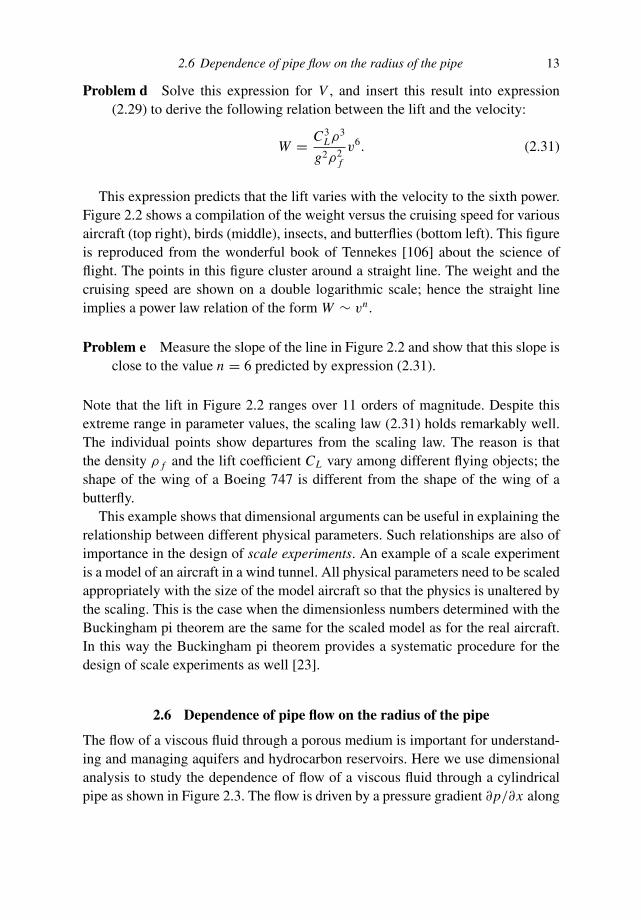
This expression predicts that the lift varies with the velocity to the sixth power.Figure 2.2 shows a compilation of the weight versus the cruising speed for variousaircraft (top right), birds (middle), insects, and butterflies (bottom left). This figureis reproduced from the wonderful book of Tennekes [106] about the science offlight. The points in this figure cluster around a straight line. The weight and thecruising speed are shown on a double logarithmic scale; hence the straight lineimplies a power law relation of the form W ∼ vn .
Problem e Measure the slope of the line in Figure 2.2 and show that this slope isclose to the value n = 6 predicted by expression (2.31).
Note that the lift in Figure 2.2 ranges over 11 orders of magnitude. Despite thisextreme range in parameter values, the scaling law (2.31) holds remarkably well.The individual points show departures from the scaling law. The reason is thatthe density ρ f and the lift coefficient CL vary among different flying objects; theshape of the wing of a Boeing 747 is different from the shape of the wing of abutterfly.
This example shows that dimensional arguments can be useful in explaining therelationship between different physical parameters. Such relationships are also ofimportance in the design of scale experiments. An example of a scale experimentis a model of an aircraft in a wind tunnel. All physical parameters need to be scaledappropriately with the size of the model aircraft so that the physics is unaltered bythe scaling. This is the case when the dimensionless numbers determined with theBuckingham pi theorem are the same for the scaled model as for the real aircraft.In this way the Buckingham pi theorem provides a systematic procedure for thedesign of scale experiments as well [23].
2.6 Dependence of pipe flow on the radius of the pipe
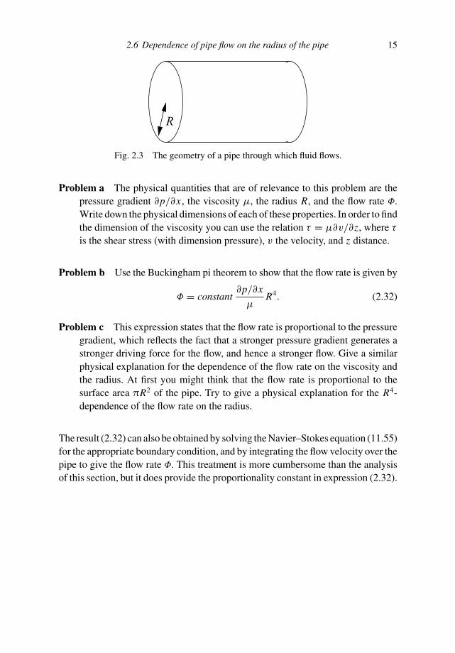
The flow of a viscous fluid through a porous medium is important for understand-ing and managing aquifers and hydrocarbon reservoirs. Here we use dimensionalanalysis to study the dependence of flow of a viscous fluid through a cylindricalpipe as shown in Figure 2.3. The flow is driven by a pressure gradient ∂p/∂x along

14 Dimensional analysis
Boeing 747
Concorde
F-14Fokker F-28Fokker F-27
Mig-23
F-16
Learjet 31
Beech King Air
Beech BaronBeech BonanzaPiper Warrior
Schleicher ASW22BSchleicher ASK23
ultralight
human-powered airplane skysurfer
pteranodon
Canada goose
pheasant
razorbill
kittiwake
common tern
Franklin’s gullpigeon hawk
Wilson’s snipestarling
purple martinhermit thrush
tree swallowbank swallow
ant lion
green-veined whitecrane fly
house flygnat
hover fly
midge
1 2 3 4 5 7 10 20 30 50 70 100 200
106
105
104
103
102
101
100
10−1
10−2
10−3
10−4
10−5
wei
ghtW
(ne
wto
ns)
cruising speed V (meters per second)
DC-10
Boeing 757Boeing 727
wandering albatrosswhite pelicangolden eagle
brown pelican
spotted sandpiper
chimney swifthouse wren
meat flyhoneybee
fruit fly
gannet
scorpion flydamsel fly
10210 103 1041
wing loading W/S (newtons per square meter)
Boeing 767
Boeing 737
Beech Airliner
mute swan
osprey
herring gullsnowy owl
partridgeruffed grouse
puffin
goshawk
American robin
English sparrow
stag beetleruby-throated hummingbird
American redstartgolden-crowned kinglet
European goldcrestprivet hawk
blue underwingcock chafer
dung beetlelittle stag beetle
summer chaferbumblebee
hornet
yellow-banded dragonflyeyed hawkcommon swallowtail
green dragonfly
cabbage white
Fig. 2.2 The weight of many flying objects (vertical axis) against their cruisingspeed (horizontal axis) on a log–log plot. This figure is reproduced from reference[106] with permission from MIT Press.
the center axis of the cylinder. We assume that the fluid has a viscosity µ, and wewant to find the relation between the strength of the flow along the pipe per unittime and the radius R. As a measure of the flow rate we use the volume of the flowper unit time, and designate this quantity with the symbol Φ.
2.6 Dependence of pipe flow on the radius of the pipe 15
R
Fig. 2.3 The geometry of a pipe through which fluid flows.
Problem a The physical quantities that are of relevance to this problem are thepressure gradient ∂p/∂x , the viscosity µ, the radius R, and the flow rate Φ.Write down the physical dimensions of each of these properties. In order to findthe dimension of the viscosity you can use the relation τ = µ∂v/∂z, where τ
is the shear stress (with dimension pressure), v the velocity, and z distance.
Problem b Use the Buckingham pi theorem to show that the flow rate is given by
Φ = constant∂p/∂x
µR4. (2.32)
Problem c This expression states that the flow rate is proportional to the pressuregradient, which reflects the fact that a stronger pressure gradient generates astronger driving force for the flow, and hence a stronger flow. Give a similarphysical explanation for the dependence of the flow rate on the viscosity andthe radius. At first you might think that the flow rate is proportional to thesurface area πR2 of the pipe. Try to give a physical explanation for the R4-dependence of the flow rate on the radius.
The result (2.32) can also be obtained by solving the Navier–Stokes equation (11.55)for the appropriate boundary condition, and by integrating the flow velocity over thepipe to give the flow rate Φ. This treatment is more cumbersome than the analysisof this section, but it does provide the proportionality constant in expression (2.32).
3
Power series
3.1 Taylor series
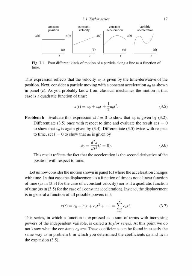
In many applications in mathematical physics it is useful to write the quantity ofinterest as a sum of a number of terms. To fix our mind, let us consider the motionof a particle that moves along a line as time progresses. The motion is completelydescribed by giving the position x(t) of the particle as a function of time. Considerthe four different types of motion that are shown in Figure 3.1.
The simplest motion is a particle that does not move, as shown in panel (a). Inthis case the position of the particle is constant:
x(t) = x0. (3.1)
The value of the parameter x0 follows by setting t = 0 in this expression; thisimmediately gives
x0 = x (0) . (3.2)
In panel (b) the situation for a particle that moves with a constant velocity is shown,thus the position is a linear function of time:
x(t) = x0 + v0t. (3.3)
Again, setting t = 0 gives the parameter x0, which is given again by (3.2). Thevalue of the parameter v0 follows by differentiating (3.3) with respect to time andby setting t = 0.
Problem a Do this and show that
v0 = dx
dt(t = 0). (3.4)
16
3.1 Taylor series 17
x(t)
t
positionconstant
(a)
x(t)
t
constant
x(t)
t
constant
x(t)
t
(c)(b) (d)
velocityvariable
acceleration acceleration
Fig. 3.1 Four different kinds of motion of a particle along a line as a function oftime.
This expression reflects that the velocity v0 is given by the time-derivative of theposition. Next, consider a particle moving with a constant acceleration a0 as shownin panel (c). As you probably know from classical mechanics the motion in thatcase is a quadratic function of time:
x(t) = x0 + v0t + 1
2a0t2. (3.5)
Problem b Evaluate this expression at t = 0 to show that x0 is given by (3.2).Differentiate (3.5) once with respect to time and evaluate the result at t = 0to show that v0 is again given by (3.4). Differentiate (3.5) twice with respectto time, set t = 0 to show that a0 is given by
a0 = d2x
dt2(t = 0). (3.6)
This result reflects the fact that the acceleration is the second derivative of theposition with respect to time.
Let us now consider the motion shown in panel (d) where the acceleration changeswith time. In that case the displacement as a function of time is not a linear functionof time (as in (3.3) for the case of a constant velocity) nor is it a quadratic functionof time (as in (3.5) for the case of a constant acceleration). Instead, the displacementis in general a function of all possible powers in t :
x(t) = c0 + c1t + c2t2 + · · · =∞
∑
n=0
cntn. (3.7)
This series, in which a function is expressed as a sum of terms with increasingpowers of the independent variable, is called a Taylor series. At this point we donot know what the constants cn are. These coefficients can be found in exactly thesame way as in problem b in which you determined the coefficients a0 and v0 inthe expansion (3.5).

18 Power series
Problem c Determine the coefficient cm by differentiating expression (3.7)m times with respect to t and by evaluating the result at t = 0 to show that
cm = 1
m!
dm x
dtm(x = 0). (3.8)
Of course there is no reason why the Taylor series can only be used to describethe displacement x(t) as a function of time t . In the literature, the Taylor seriesis frequently used to describe a function f (x) that depends on x . Of course it isimmaterial what we call a function. By making the replacements x → f and t → xexpressions (3.7) and (3.8) can also be written as:
f (x) =∞
∑
n=0
cnxn, (3.9)
with
cn = 1
n!
dn f
dxn(x = 0). (3.10)
You may also find this result in the literature written as
f (x) =∞
∑
n=0
xn
n!
dn f
dxn(x = 0) = f (0) + x
d f
dx(x = 0) + x2
2
d2 f
dx2(x = 0) + · · · .
(3.11)
Problem d By evaluating the derivatives of f (x) at x = 0 show that the Taylorseries of the following functions are given by:
sin (x) = x − 1
3!x3 + 1
5!x5 − · · · ; (3.12)
cos (x) = 1 − 1
2x2 + 1
4!x4 − · · · ; (3.13)
ex = 1 + x + 1
2!x2 + 1
3!x3 + · · · =
∞∑
n=0
1
n!xn; (3.14)
1
1 − x= 1 + x + x2 + · · · =
∞∑
n=0
xn; (3.15)
(1 − x)α = 1 − αx + 1
2!α (α − 1) x2 − 1
3!α (α − 1) (α − 2) x3 + · · · . (3.16)
Up to this point we made the Taylor expansion around the point x = 0. How-ever, one can make a Taylor expansion of f (x + h) around any arbitrary point x .
3.1 Taylor series 19
The associated Taylor series can be obtained by replacing the distance x that wemove from the expansion point by a distance h and by replacing the expansionpoint 0 by x . Making the replacements x → h and 0 → x expansion (3.11) isgiven by
f (x + h) =∞
∑
n=0
hn
n!
dn f
dxn(x). (3.17)
Problem e Truncate this series after the second term and show that this leads tothe following approximations:
f (x + h) − f (x) ≈ hd f
dx(x), (3.18)
d f
dx≈ f (x + h) − f (x)
h. (3.19)
These expressions may appear to be equivalent in a trivial way. However, we willmake extensive use of them in different ways. Equation (3.18) makes it possible toestimate the change in a function when the independent variable is changed slightly,whereas (3.19) is useful for estimating the derivative of a function given its valuesat neighboring points. The issue of estimating the derivative of a function is treatedin much more detail in Section 12.2. Figure 12.2 makes it possible to also derivethe estimate (3.19) geometrically by using that the derivative of a function is justthe slope of that function.
The Taylor series can also be used for functions of more than onevariable. As an example consider a function f (x, y) that depends on the variablesx and y. The generalization of the Taylor series (3.9) to functions of two variablesis given by
f (x, y) =∞
∑
n,m=0
cnmxn ym . (3.20)
At this point the coefficients cnm are not yet known. They follow in the same way asthe coefficients of the Taylor series of a function that depends on a single variableby taking the partial derivatives of the Taylor series and evaluating the result at thepoint where the expansion is made.
Problem f Take all the partial derivatives of (3.20) with respect to x and y upto second order, including the mixed derivative ∂2 f/∂x∂y, and evaluate theresult at the expansion point x = y = 0 to show that up to second order the

20 Power series
Taylor expansion (3.20) is given by
f (x, y) = f (0, 0) + ∂ f
∂x(0, 0) x + ∂ f
∂y(0, 0) y
+ 1
2
∂2 f
∂x2(0, 0) x2 + ∂2 f
∂x∂y(0, 0) xy
+ 1
2
∂2 f
∂y2(0, 0) y2 + · · · . (3.21)
Problem g This is the Taylor expansion of f (x, y) around the point x = y = 0.Make suitable substitutions in this result to show that the Taylor expansionaround an arbitrary point (x, y) is given by
f (x + hx , y + hy) = f (x, y) + ∂ f
∂x(x, y) hx + ∂ f
∂y(x, y) hy
+ 1
2
∂2 f
∂x2(x, y) h2
x + ∂2 f
∂x∂y(x, y) hx hy
+ 1
2
∂2 f
∂y2(x, y) h2
y + · · · . (3.22)
Let us return to the Taylor series (3.9) with the coefficients cm given by (3.10).This series hides an intriguing result. Equations (3.9) and (3.10) suggest that afunction f (x) is specified for all values of its argument x when all the derivativesare known at a single point x = 0. This means that the global behavior of a functionis completely contained in the properties of the function at a single point. In fact,this is not always true.
First, the series (3.9) is an infinite series, and the sum of infinitely many termsdoes not necessarily lead to a finite answer. As an example look at the series (3.15).A series can only converge when the terms go to zero as n → ∞, because otherwiseevery additional term changes the sum. The terms in the series (3.15) are given byxn; these terms only go to zero as n → ∞ when |x | < 1. In general, the Taylorseries (3.9) only converges when x is smaller than a certain critical value called theradius of convergence. Details on the criteria for the convergence of series can befound in for example Boas [19] or Butkov [24].
The second reason why the derivatives at one point do not necessarily constrainthe function everywhere is that a function may change its character over the rangeof parameter values that is of interest. As an example let us return to a movingparticle and consider a particle at position x(t) that is at rest until a certain time t0

3.1 Taylor series 21
t
x(t)
Fig. 3.2 The motion of a particle that suddenly changes character at time t0.
and that then starts moving with a uniform velocity v = 0:
x(t) =
x0 for t ≤ t0x0 + v(t − t0) for t > t0
. (3.23)
The motion of the particle is sketched in Figure 3.2. A straightforward application of(3.8) shows that all the coefficients cn of this function vanish except c0 which is givenby x0. The Taylor series (3.7) is therefore given by x(t) = x0 which clearly differsfrom (3.23). The reason for this is that the function (3.23) changes its character att = t0 in such a way that nothing in the behavior for times t < t0 predicts the suddenchange in the motion at time t = t0. Mathematically things go wrong because thefirst and higher derivatives of the function are not defined at time t = t0.
Problem h What is the first derivative of x(t) just to the left and just to the rightof t = t0 ? What is the second derivative at that point?
The function (3.23) is said to be not analytic at the point t = t0. The issue of analyticfunctions is treated in more detail in Sections 16.1 and 17.1.
Problem i Try to compute the Taylor series of the function x(t) = 1/t using (3.7)and (3.8). Draw this function and explain why the Taylor series cannot be usedfor this function.
Problem j Do the same for the function x(t) = √t .
The examples in the last two problems show that when a function is not analyticat a certain point, the coefficients of the Taylor series are not defined. This signalsthat such a function cannot be represented by a Taylor series around that point.
Frequently the result of a calculation can be obtained by summing a series. InSection 3.3 this is used to study the behavior of a bouncing ball. The bounces
22 Power series
are “natural” units for analyzing the problem at hand. In Section 3.4 the re-verse is done when studying the total reflection of a stack of reflective layers.In this case a series expansion actually gives physical insight into a complexexpression.
3.2 Growth of the Earth by cosmic dust
In this section we use the growth of the Earth by the accretion of cosmic dust as anexample to illustrate the usefulness of the (first order) Taylor series. The Earth iscontinuously bombarded from space by meteorites. Some of these meteorites canbe large and lead to massive impact craters. As an example the gravity anomalyover the Chicxulub impact crater in Mexico is shown in Figure 21.1. The diameterof this impact crater is about 100 km. However, the bulk of the cosmic dust that fallsfrom space onto the Earth is in the form of many small particles. The total mass ofall the cosmic dust that falls on the Earth is estimated by Love and Brownlee [65]to be approximately 5 × 10⁷ kg/a. (The unit “a” stands for annum (or year); thismeans that the unit used here is kilograms per year.) This estimate, however, is notvery accurate and we can probably only trust the first decimal of this number. Thismeans that in subsequent calculations it is pointless to aim for an accuracy of morethan one significant figure.
Since the cosmic dust increases the mass of the Earth, the size of the Earth willincrease. In this section we determine the growth of the Earth’s radius per year dueto the bombardment of our planet by cosmic dust.
Problem a Assuming that a density of meteorites is given by ρ =2.5 × 10³ kg/m3 [65] show that the annual growth of the volume of the Earthis given by
δV = 2 × 10⁴ m3. (3.24)
Also show that this corresponds to a block of (27 × 27 × 27) m3.
We assume that the Earth is a perfect sphere so that the volume and the radius r ofthe Earth are related by the relation
V = 4π
3r3. (3.25)
From this relation we can deduce that the annual change δr of the radius of theEarth can be computed from the expression
δr =[
3 (V + δV )
4π
]1/3
−(
3V
4π
)1/3
. (3.26)
3.2 Growth of the Earth by cosmic dust 23
Problem b Assume the Earth’s radius is given by r = 7000 km. Insert this numberand the value of δV from expression (3.24) into (3.26) and use a calculator tocompute the increase, δr , of the radius of the Earth.
You have probably found that the annual increase in the Earth’s radius is equalto zero. This cannot be true because we know that δV is not equal to zero. Thereason that your calculator has given you a wrong answer is that in (3.26) we aresubtracting two very large numbers that differ by a small amount. The volume V ofthe Earth is of the order 1021 m3 while according to (3.24) the annual increase of thevolume is of the order 104 m3. Most calculators carry out all the calculations with arelatively small number of digits; most use between 6 and 10 decimals. When yousubtract two numbers that are very large and that have a very small difference, thisdifference will be truncated after say 6 or 10 decimals. In our problem, the first tendecimals of both terms in (3.26) are identical, hence your calculator tells you thatthe radius of the Earth is not growing because of the accretion of cosmic dust.
In general, subtracting two large numbers that have a difference that is muchsmaller leads to numerical inaccuracies. Clearly a trick is needed to obtain thedesired growth of the Earth’s radius. The cause of this problem is that the annualchange in the volume is so small. We can turn this problem to our advantage byusing that the Taylor series that we introduced in the previous section is extremelyaccurate when the independent variable is changed by a very small amount. Herewe will compute the increase of the Earth’s radius using expression (3.18).
Problem c Show that this expression can also be written as
δ f ≈ ∂ f
∂xδx, (3.27)
where δ f is the change in the function f (x) due to a change δx in the inde-pendent variable x .
Problem d Apply this result to the function r (V ) = (3V/4π)1/3 that gives theradius as a function of the volume to derive that
δr = 1
3rδV
V. (3.28)
Problem e Use this result to compute the annual increase of the radius of theEarth due to the accretion of cosmic dust and show that the result is of theorder of 1 angstrom per year (1 angstrom is 10−10 m).
Problem f Can you think of an object that is the size of 1 angstrom?

24 Power series
Problem g How much has the Earth’s radius increased over the age of the Earth?In this calculation you may assume that the age of the Earth is 4.5 billion years.
The upshot of this calculation is that the growth of the Earth due to the present-day accretion of cosmic dust is negligible. However, the technique of using thefirst order Taylor series to determine the small change in a quantity is extremelypowerful. In fact, you have encountered in this section an example that demonstratesthat an approximation can provide a more meaningful answer than a calculationcarried out using a calculator or computer.
3.3 Bouncing ball
In this section we study a rubber ball that bounces on a flat surface and slowlycomes to rest as sketched in Figure 3.3. You will know from experience that theball bounces more and more rapidly with time. The question we address here iswhether the ball can actually bounce infinitely many times in a finite amount oftime. This problem is not an easy one. In general with large difficult problems it isa useful strategy to divide the large and difficult problem that you cannot solve intosmaller and simpler problems that you can solve. By assembling these smaller sub-problems one can then often solve the large problem. This is exactly what we willdo here. First we will find how much time it takes for the ball to bounce once givenits velocity. Given a prescription of the energy loss in one bounce we will determinea relation between the velocity of subsequent bounces. From these ingredients wecan determine the relation between the times needed for subsequent bounces. Bysumming this series over an infinite number of bounces we can determine the totaltime that the ball has bounced. Keep this general strategy in mind when solvingcomplex problems. Almost all of us are better at solving a number of small problemsrather than a single large problem!
. . .
Fig. 3.3 The motion of a bouncing ball that loses energy with every bounce. Tovisualize the motion of the ball better, the ball is a given a constant horizontalvelocity that is conserved during the bouncing.
3.3 Bouncing ball 25
Problem a A ball moves upward from the level z = 0 with velocity v andis subject to a constant gravitational acceleration g. Determine the heightthe ball reaches and the time it takes for the ball to return to its startingpoint.
At this point we have determined the relevant properties for a single bounce. Duringeach bounce the ball loses energy due to the fact that the ball is deformed inelasticallyduring the bounce. We assume that during each bounce the ball loses a fraction γ
of its energy.
Problem b Let the velocity at the beginning of the nth bounce be vn . Show thatwith the assumed rule for energy loss this velocity is related to the velocityvn−1 of the previous bounce by
vn =√
1 − γ vn−1. (3.29)
Hint: when the ball bounces upward from z = 0 all its energy is kinetic energy12 mv2.
In problem a you determined the time it took the ball to bounce once, given theinitial velocity, while expression (3.29) gives a recursive relation for the velocitybetween subsequent bounces. In problem a you also computed the time that ittakes to carry out a single bounce. By assembling these results we can find arelation between the time tn for the nth bounce and the time tn−1 for the previousbounce.
Problem c Determine this relation. In addition, let us assume that the ball isthrown up the first time from z = 0 to reach a height z = H . Compute thetime t0 needed for the ball to make the first bounce and combine these resultsto show that
tn =√
8H
g(1 − γ )n/2, (3.30)
where g is the acceleration of gravity.
We can use this expression to determine the total time TN it takes to carry out Nbounces. This time is given by TN = ∑N
n=0 tn . By setting N equal to infinity wecan compute the time T∞ it takes to bounce infinitely often.
26 Power series
Problem d Determine this time by carrying out the summation and show that itis given by:
T∞ =√
8H
g
1
1 − √1 − γ
. (3.31)
Hint: write (1 − γ )n/2 as(√
1 − γ)n
and treat√
1 − γ as the parameter x inthe appropriate Taylor series of Section 3.1.
This result shows that the time it takes to bounce infinitely often is indeed finite.For the special case that the ball loses no energy, γ = 0 and T∞ is infinite. Thisreflects that a ball that loses no energy will bounce forever.
Expression (3.31) looks messy. It often happens in mathematical physics thatthe final expression resulting from a calculation is so complex that it is difficult tounderstand it. However, often we know that certain terms in an expression can beassumed to be very small (or very large). This may allow us to obtain an approximateexpression that is of a simpler form. In this way we trade accuracy for simplicityand understanding. In practice, this often turns out to be a good deal! In our exampleof the bouncing ball we assume that the energy loss at each bounce is small, that isthat γ is small.
Problem e Show that in this case T∞ ≈ √(8H/g) 2/γ by using the leading terms
of the appropriate Taylor series of Section 3.1.
This result is actually quite useful. It tells us how the total bounce time approachesinfinity when the energy loss γ goes to zero.
In this example we have solved the problem in little steps. In general we takelarger steps in the problems in this book, and you will have to discover how todivide a large step into smaller steps. The next problem is a “large” problem; solveit by dividing it into smaller problems. First formulate the smaller problems asingredients for the large problem before you actually start working on the smallerproblems.
Make it a habit whenever you are solving problems to first formulate astrategy for how you are going to attack a problem before you actuallystart working on the sub-problems. Make a list if this helps you and donot be deterred if you cannot solve a particular sub-problem. Perhapsyou can solve the other sub-problems and somebody else can help youwith the one you cannot solve.
Keeping this in mind, solve the following “large” problem:

3.4 Reflection and transmission by a stack of layers 27
Problem f Let the total distance traveled by the ball in the vertical direction duringinfinitely many bounces be denoted by S. Show that S = 2H/γ .
3.4 Reflection and transmission by a stack of layers
In 1917 Lord Rayleigh [86] addressed the question of why some birds and in-sects have beautiful iridescent colors. He explained this by studying the reflectiveproperties of a stack of thin reflective layers. This problem is also of interest ingeophysics; in exploration seismology one is also interested in the reflection andtransmission properties of stacks of reflective layers in the Earth. Lord Rayleighsolved this problem in the following way.
Suppose we have one stack of layers on the left with reflection coefficient RL andtransmission coefficient TL and another stack of layers on the right with reflectioncoefficient RR and transmission coefficient TR . If we add these two stacks together toobtain a larger stack of layers, what are the reflection coefficient R and transmissioncoefficient T of the total stack of layers? See Figure 3.4 for the scheme of thisproblem. The reflection coefficient is defined as the ratio of the strengths of thereflected and the incident waves, similarly the transmission coefficient is defined asthe ratio of the strengths of the transmitted wave and the incident wave. To highlightthe essential arguments we simplify the analysis and ignore that the reflectioncoefficient for waves incident from the left and the right are in general not thesame. However, this simplification does not change the essence of the comingarguments.
Before we start solving the problem, let us speculate what the transmission coef-ficient of the combined stack is. It may seem natural to assume that the transmission
R
1
B
A
T
L(eft) R(ight)
Fig. 3.4 Geometry of the problem where stacks of n and m reflective layers arecombined. The notation of the strength of left- and right-going waves is indicated.

28 Power series
coefficient of the combined stack is the product of the transmission coefficient ofthe individual stacks:
T?= TL TR. (3.32)
However, this result is wrong and we will discover why this is so. ConsiderFigure 3.4 again. The unknown quantities are R, T , and the coefficients A andB for the right-going and left-going waves between the stacks. An incident wavewith strength 1 impinges on the stack from the left. Let us first determine thecoefficient A of the right-going waves between the stacks. The right-going wavebetween the stacks contains two contributions: the wave transmitted from the left(this contribution has a strength 1 × TL ) and the wave reflected towards the rightdue the incident left-going wave with strength B (this contribution has a strengthB × RL). This implies that:
A = TL + B RL . (3.33)
Problem a Using similar arguments show that:
B = ARR, (3.34)
T = ATR, (3.35)
R = RL + BTL . (3.36)
This is all we need to solve our problem. The system of equations (3.33)–(3.36)consists of four linear equations with four unknowns A, B, R, and T . We couldsolve this system of equations by brute force, but some thought will make life easierfor us. Note that the last two equations immediately give T and R once A and B areknown. The first two equations give A and B.
Problem b Show that
A = TL
(1 − RL RR), (3.37)
B = TL RR
(1 − RL RR). (3.38)
This is a puzzling result, the right-going wave A between the layers not onlycontains the transmission coefficient of the left layer TL but also an additional term1/(1 − RL RR).
Problem c Make a series expansion of 1/(1 − RL RR) in the quantity RL RR andshow that this term accounts for the waves that bounce back and forth betweenthe two stacks. Hint: use that RL is the reflection coefficient for a wave that
3.4 Reflection and transmission by a stack of layers 29
reflects from the left stack and RR is the reflection coefficient for one thatreflects from the right stack so that RL RR is the total reflection coefficient fora wave that bounces once between the left and the right stacks.
This implies that the term 1/(1 − RL RR) accounts for the waves that bounce backand forth between the two stacks of layers. It is for this reason that we call this areverberation term. It plays an important role in computing the response of layeredmedia.
Problem d Show that the reflection and transmission coefficients of the combinedstack of layers are given by:
R = RL + T 2L RR
(1 − RL RR), (3.39)
T = TL TR
(1 − RL RR). (3.40)
At the beginning of this section we conjectured that the transmission coefficient ofthe combined stacks is the product of the transmission coefficient of the separatestacks, see expression (3.32).
Problem e Is this conjecture correct? Under which conditions is it approximatelycorrect?
Equations (3.39) and (3.40) are useful for computing the reflection and transmis-sion coefficients of a large stack of layers. The reason for this is that it is extremelysimple to determine the reflection and transmission coefficients of a very thin layerusing the Born approximation. (The Born approximation is treated in Section 23.2.)Let the reflection and transmission coefficients of a single thin layer n be denotedby rn and tn respectively and let the reflection and transmission coefficients of astack of n layers be denoted by Rn and Tn respectively. Suppose that the left stackconsists of n layers and that we want to add an (n + 1)th layer to the stack. Inthat case the right stack consists of a single (n + 1)th layer so that RR = rn+1 andTR = tn+1 and the reflection and transmission coefficients of the left stack are givenby RL = Rn , TL = Tn . Using this in expressions (3.39) and (3.40) yields
Rn+1 = Rn + T 2n rn+1
(1 − Rnrn+1), (3.41)
Tn+1 = Tntn+1
(1 − Rnrn+1). (3.42)
30 Power series
This means that given the known response of a stack of n layers, one can easilycompute the effect of adding the (n + 1)th layer to this stack. In this way one canrecursively build up the response of the complex reflector out of the known responseof very thin reflectors. Computers are pretty stupid, but they are ideally suited forapplying the rules (3.41) and (3.42) a large number of times. Of course this processhas to be begun with a medium in which no layers are present.
Problem f What are the reflection coefficient R0 and the transmission coefficientT0 when there are as yet no reflective layers present? Describe how one cancompute the response of a thick stack of layers once we know the response ofa very thin layer.
In developing this theory, Lord Rayleigh prepared the foundations for a theory thatlater became known as invariant embedding which turns out to be extremely usefulfor a number of scattering and diffusion problems [13, 109].
The main conclusion of the treatment of this section is that the transmission of acombination of two stacks of layers is not the product of the transmission coefficientsof the two separate stacks because the waves that repeatedly reflect between thetwo stacks leave an imprint on the transmission coefficient as well. Paradoxically,Berry and Klein [15] showed in their analysis of “transparent mirrors” that forthe special case of a large stack of layers with random transmission coefficientthe total transmission coefficient is the product of the transmission coefficientsof the individual layers, despite the fact that multiple reflections play a crucial rolein this process.
4
Spherical and cylindrical coordinates
Many problems in mathematical physics exhibit a spherical or cylindrical symme-try. For example, the gravity field of the Earth is to first order spherically symmetric.Waves excited by a stone thrown into water are usually cylindrically symmetric.Although there is no reason why problems with such a symmetry cannot be ana-lyzed using Cartesian coordinates (i.e. (x, y, z)-coordinates), it is usually not veryconvenient to use such a coordinate system. The reason for this is that the theory isusually much simpler when one selects a coordinate system with symmetry prop-erties that are the same as the symmetry properties of the physical system that onewants to study. It is for this reason that spherical coordinates and cylindrical coor-dinates are introduced in this section. It takes a certain effort to become acquaintedwith these coordinate systems, but this effort is well spent because it makes solvinga large class of problems much easier.
4.1 Introducing spherical coordinates
In Figure 4.1 a Cartesian coordinate system with its x-, y-, and z-axes is shown aswell as the location of a point r. This point can be described either by its x-, y-,and z-components or by the radius r and the angles θ and ϕ shown in Figure 4.1. Inthe latter case one uses spherical coordinates. Comparing the angles θ and ϕ withthe geographical coordinates that define a point on the globe one sees that ϕ can becompared with longitude and θ can be compared with colatitude, which is definedas (latitude − 90 degrees).
Problem a The city of Utrecht in the Netherlands is located at 52 degrees northand 5 degrees east. Show that the angles θ and ϕ (in radians) that correspondto this point on the sphere are given by θ = 0.663 radians, and ϕ = 0.087radians.
31
32 Spherical and cylindrical coordinates
^
^
x-axis
y-axis
z-axis
(x,y,z)
.
.r
r
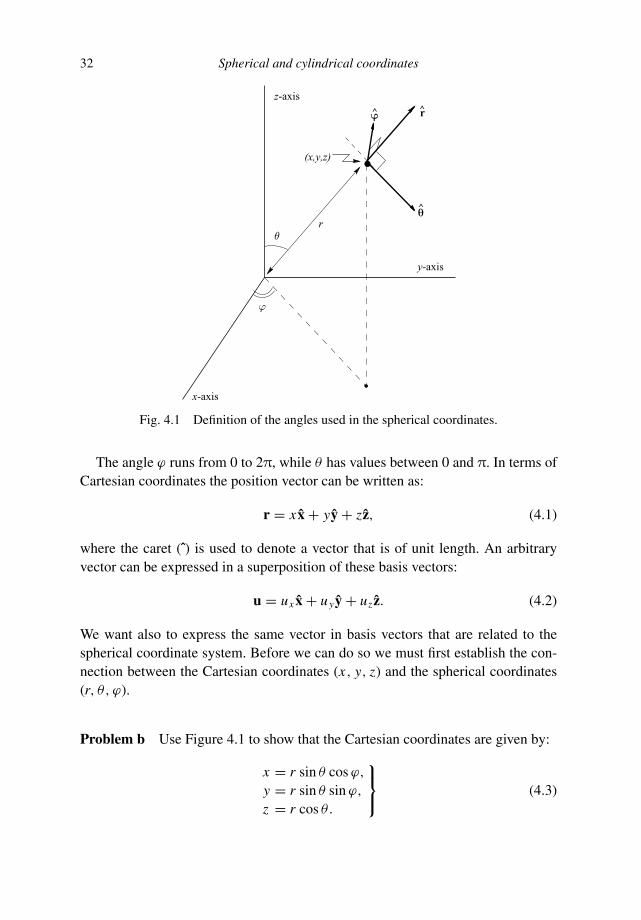
Fig. 4.1 Definition of the angles used in the spherical coordinates.
The angle ϕ runs from 0 to 2π, while θ has values between 0 and π. In terms ofCartesian coordinates the position vector can be written as:
r = x x + yy + zz, (4.1)
where the caret (ˆ) is used to denote a vector that is of unit length. An arbitraryvector can be expressed in a superposition of these basis vectors:
u = ux x + uy y + uz z. (4.2)
We want also to express the same vector in basis vectors that are related to thespherical coordinate system. Before we can do so we must first establish the con-nection between the Cartesian coordinates (x, y, z) and the spherical coordinates(r, θ, ϕ).
Problem b Use Figure 4.1 to show that the Cartesian coordinates are given by:
x = r sin θ cos ϕ,
y = r sin θ sin ϕ,
z = r cos θ.
⎫
⎬
⎭
(4.3)

4.1 Introducing spherical coordinates 33
Problem c Use these expressions to derive the following expression for the spher-ical coordinates in terms of the Cartesian coordinates:
r =√
x2 + y2 + z2,
θ = arccos(
z/√
x2 + y2 + z2)
,
ϕ = arctan (y/x) .
⎫
⎪
⎬
⎪
⎭
(4.4)
We have now obtained the relation between the Cartesian coordinates (x, y, z)and the spherical coordinates (r, θ, ϕ). Suppose we want to express the vector u ofequation (4.2) in spherical coordinates:
u = ur r + uθ θ + uϕϕ, (4.5)
and we want to know the relation between the components (ux , uy, uz) in Carte-sian coordinates and the components (ur , uθ , uϕ) of the same vector expressed inspherical coordinates. In order to do this we first need to determine the unit vectorsr, θ, and ϕ. In Cartesian coordinates, the unit vector x points along the x-axis.This is a different way of saying that it is a unit vector pointing in the directionof increasing values of x for constant values of y and z; in other words, x can bewritten as: x = ∂r/∂x .
Problem d Verify this by showing that the differentiation x = ∂r/∂x leads to the
correct unit vector in the x-direction: x =⎛
⎝
100
⎞
⎠.
Now consider the unit vector θ. Using the same argument as for the unit vector xwe know that θ is directed towards increasing values of θ for constant values of rand ϕ. This means that θ can be written as θ = C∂r/∂θ. The constant C followsfrom the requirement that θ is of unit length.
Problem e Use this reasoning for all the unit vectors r, θ and ϕ and expression(4.3) to show that:
r = ∂r∂r
, θ = 1
r
∂r∂θ
, ϕ = 1
r sin θ
∂r∂ϕ
, (4.6)
and that this result can also be written as
r =⎛
⎝
sin θ cos ϕ
sin θ sin ϕ
cos θ
⎞
⎠ , θ =⎛
⎝
cos θ cos ϕ
cos θ sin ϕ
− sin θ
⎞
⎠ , ϕ =⎛
⎝
− sin ϕ
cos ϕ
0
⎞
⎠ . (4.7)
These equations give the unit vectors r, θ and ϕ in Cartesian coordinates.
34 Spherical and cylindrical coordinates
On the right-hand side of (4.6) the derivatives of the position vector are dividedby 1, r , and r sin θ respectively. These factors are usually shown in the followingnotation:
hr = 1, hθ = r, hϕ = r sin θ. (4.8)
These scale factors play an important role in the general theory of curvilinearcoordinate systems, see Butkov [24] for details. The material presented in theremainder of this chapter as well as the derivation of vector calculus in sphericalcoordinates can be based on the scale factors given in (4.8). However, this approachwill not be taken here.
Problem f Verify explicitly that the vectors r, θ, and ϕ defined in this way forman orthonormal basis, that is they are of unit length and perpendicular to eachother:
(r · r) =(
θ · θ)
= (
ϕ · ϕ) = 1, (4.9)
(
r · θ)
= (
r · ϕ) =
(
θ · ϕ)
= 0. (4.10)
The dot denotes the inner product of two vectors.
Problem g Using expressions (4.7) for the unit vectors r, θ, and ϕ show bycalculating the cross-products explicitly that
r × θ = ϕ, θ × ϕ = r, ϕ × r = θ. (4.11)
The Cartesian basis vectors x, y, and z point in the same direction at every pointin space. This is not true for the spherical basis vectors r, θ, and ϕ; for differentvalues of the angles θ and ϕ these vectors point in different directions. This impliesthat these unit vectors are functions of both θ and ϕ. For several applications itis necessary to know how the basis vectors change with θ and ϕ. This change isdescribed by the derivative of the unit vectors with respect to the angles θ and ϕ.
Problem h Show by direct differentiation of expressions (4.7) that the derivativesof the unit vectors with respect to the angles θ and ϕ are given by:
∂ r/∂θ = θ, ∂ r/∂ϕ = sin θ ϕ,
∂θ/∂θ = −r, ∂θ/∂ϕ = cos θ ϕ,
∂ϕ/∂θ = 0, ∂ϕ/∂ϕ = − sin θ r − cos θ θ.
⎫
⎬
⎭
(4.12)

4.2 Changing coordinate systems 35
4.2 Changing coordinate systems
Now that we have derived the properties of the unit vectors r, θ, and ϕ, we are inthe position to derive how the components (ur , uθ , uϕ) of the vector u defined inequation (4.5) are related to the usual Cartesian coordinates (ux , uy, uz). This canmost easily be achieved by writing expressions (4.7) in the following form:
r = sin θ cos ϕ x + sin θ sin ϕ y + cos θ z,θ = cos θ cos ϕ x + cos θ sin ϕ y − sin θ z,ϕ = − sin ϕ x + cos ϕ y.
⎫
⎬
⎭
(4.13)
Problem a Convince yourself that this expression can also be written in a sym-bolic form as
⎛
⎝
rθ
ϕ
⎞
⎠ = M
⎛
⎝
xyz
⎞
⎠ , (4.14)
with the matrix M given by
M =⎛
⎝
sin θ cos ϕ sin θ sin ϕ cos θ
cos θ cos ϕ cos θ sin ϕ − sin θ
− sin ϕ cos ϕ 0
⎞
⎠ . (4.15)
Of course expression (4.14) can only be considered to be a shorthand notation forequations (4.13) since the entries in (4.14) are vectors rather than single components.
The relation between the spherical components (ur , uθ , uϕ) and the Cartesiancomponents (ux , uy, uz) of the vector u can be obtained by inserting expressions(4.13) for the spherical coordinate unit vectors into the relation u = ur r + uθ θ +uϕϕ.
Problem b Do this and collect together all terms multiplying the unit vectors x,y and z to show that expression (4.5) for the vector u is equivalent to:
u = (
ur sin θ cos ϕ + uθ cos θ cos ϕ − uϕ sin ϕ)
x
+ (
ur sin θ sin ϕ + uθ cos θ sin ϕ + uϕ cos ϕ)
y
+ (ur cos θ − uθ sin θ ) z. (4.16)
Problem c Show that this relation can also be written as:⎛
⎝
ux
uy
uz
⎞
⎠ = MT
⎛
⎝
ur
uθ
uϕ
⎞
⎠ , (4.17)
36 Spherical and cylindrical coordinates
where the matrix M is given by (4.15). In this expression, MT is the transposeof the matrix M; that is it is the matrix obtained by interchanging rows andcolumns of the matrix MT
i j = M ji .
We have not yet reached with equation (4.17) our goal of expressing the sphericalcoordinate components (ur , uθ , uϕ) of the vector u in the Cartesian components(ux , uy, uz). This is most easily achieved by multiplying (4.17) with the inversematrix (MT )−1, which gives:
⎛
⎝
ur
uθ
uϕ
⎞
⎠ = (
MT)−1
⎛
⎝
ux
uy
uz
⎞
⎠ . (4.18)
However, now we have only shifted the problem because we do not know theinverse (MT )−1. We could of course painstakingly compute this inverse, but thiswould be a laborious process that we can avoid. It follows by inspection of (4.15)that all the columns of M are of unit length and that the columns are orthogonal.This implies that M is an orthogonal matrix. Orthogonal matrices have the usefulproperty that the transpose of the matrix is identical to the inverse of the matrix:M−1 = MT .
Problem d The property M−1 = MT can be verified explicitly by showing thatMMT and MT M are equal to the identity matrix; do this!
Note that we have obtained the inverse of the matrix by making a guess andby verifying that this guess indeed solves our problem. This approach is oftenvery useful in solving mathematical problems; there is nothing wrong with mak-ing a guess as long as you check afterwards that your guess is indeed a solu-tion to your problem. Since we know that M−1 = MT , it follows that (MT )−1 =(M−1)−1 = M.
Problem e Use these results to show that the spherical coordinate componentsof u are related to the Cartesian coordinates by the following transformationrule:
⎛
⎝
ur
uθ
uϕ
⎞
⎠ =⎛
⎝
sin θ cos ϕ sin θ sin ϕ cos θ
cos θ cos ϕ cos θ sin ϕ − sin θ
− sin ϕ cos ϕ 0
⎞
⎠
⎛
⎝
ux
uy
uz
⎞
⎠ . (4.19)

4.3 Acceleration in spherical coordinates 37
4.3 Acceleration in spherical coordinates
You may wonder whether we really need all these transformation rules between aCartesian coordinate system and a system of spherical coordinates. The answer isyes! An important example can be found in meteorology where air moves along aspherical surface. The velocity v of the air can be expressed in spherical coordinatesas:
v =vr r + vθ θ + vϕϕ. (4.20)
The motion of the air is governed by Newton’s law, but when the velocity v and theforce F are both expressed in spherical coordinates it would be wrong to expressthe θ -component of Newton’s law as: ρdvθ/dt = Fθ . The reason is that the basisvectors of the spherical coordinate system depend on the position. When a particlemoves, the directions of the basis vectors change as well. This is a different wayof saying that the spherical coordinate system is not a Cartesian system where theorientation of the coordinate axes is independent of the position. When computingthe acceleration in such a system additional terms appear that account for the factthat the coordinate system is curvilinear. The results of Section 4.1 contain all theingredients we need.
Let us follow a particle moving over a sphere. The position vector r has anobvious expansion in spherical coordinates:
r = r r. (4.21)
The velocity is obtained by taking the time-derivative of this expression. However,the unit vector r is a function of the angles θ and ϕ, see equation (4.7). This meansthat when we take the time-derivative of (4.21) to obtain the velocity we also need todifferentiate r with time. Note that this is not the case with the Cartesian expressionr = x x + yy + zz because the unit vectors x, y, and z are constant, hence they donot change when the particle moves and they thus have a vanishing time-derivative.
As an example, let us compute the time-derivative of r. This vector is a functionof θ and ϕ, and these angles both change with time as the particle moves. Usingthe chain rule it thus follows that:
d rdt
= d r(θ, ϕ)
dt= dθ
dt
∂ r∂θ
+ dϕ
dt
∂ r∂ϕ
. (4.22)
The derivatives ∂ r/∂θ and ∂ r/∂ϕ can be eliminated with (4.12).
Problem a Use expressions (4.12) to eliminate the derivatives ∂ r/∂θ and ∂ r/∂ϕ
and carry out a similar analysis for the time-derivatives of the unit vectors θ

38 Spherical and cylindrical coordinates
and ϕ to show that:
d rdt
= θ θ + sin θ ϕ ϕ,
dθ
dt= −θ r + cos θ ϕ ϕ,
dϕ
dt= − sin θ ϕ r − cos θ ϕ θ.
⎫
⎪
⎪
⎪
⎪
⎪
⎪
⎬
⎪
⎪
⎪
⎪
⎪
⎪
⎭
(4.23)
In these and other expressions in this section a dot is used to denote the time-derivative: F ≡ d F/dt .
Problem b Use (4.21), the first line of (4.23) and the definition v = dr/dt toshow that in spherical coordinates:
v = r r + r θ θ + r sin θ ϕ ϕ. (4.24)
In spherical coordinates the components of the velocity are thus given by:
vr = r ,
vθ = r θ ,
vϕ = r sin θ ϕ.
⎫
⎬
⎭
(4.25)
This result can be interpreted geometrically. As an example, let us consider the radialcomponent of the velocity, see Figure 4.2. To obtain the radial component of thevelocity we keep the angles θ and ϕ fixed and let the radius r (t) change to r (t + t)over a time t . The particle has moved a distance r (t + t) − r (t) = (dr/dt)/tin a time t , so that the radial component of the velocity is given by vr = dr/dt = r .This is the result given by the first line of (4.25).
Problem c Use similar geometric arguments to explain the form of the velocitycomponents vθ and vϕ given in (4.25).
Problem d We are now in the position to compute the acceleration in sphericalcoordinates. To do this differentiate (4.24) with respect to time and use ex-pression (4.23) to eliminate the time-derivatives of the basis vectors. Use thisto show that the acceleration a is given by:
a = (
vr − θvθ − sin θ ϕvϕ
)
r
+ (
vθ + θvr − cos θ ϕvϕ
)
θ
+ (
vϕ + sin θ ϕvr + cos θ ϕvθ
)
ϕ. (4.26)
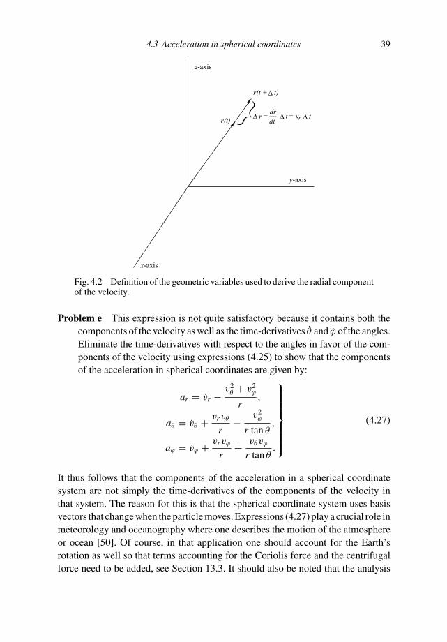
4.3 Acceleration in spherical coordinates 39
∆ tr(t + )
r∆ ∆ t ∆ trv= =drdt
x-axis
y-axis
z-axis
r(t)
Fig. 4.2 Definition of the geometric variables used to derive the radial componentof the velocity.
Problem e This expression is not quite satisfactory because it contains both thecomponents of the velocity as well as the time-derivatives θ and ϕ of the angles.Eliminate the time-derivatives with respect to the angles in favor of the com-ponents of the velocity using expressions (4.25) to show that the componentsof the acceleration in spherical coordinates are given by:
ar = vr − v2θ + v2
ϕ
r,
aθ = vθ + vrvθ
r− v2
ϕ
r tan θ,
aϕ = vϕ + vrvϕ
r+ vθvϕ
r tan θ.
⎫
⎪
⎪
⎪
⎪
⎪
⎪
⎬
⎪
⎪
⎪
⎪
⎪
⎪
⎭
(4.27)
It thus follows that the components of the acceleration in a spherical coordinatesystem are not simply the time-derivatives of the components of the velocity inthat system. The reason for this is that the spherical coordinate system uses basisvectors that change when the particle moves. Expressions (4.27) play a crucial role inmeteorology and oceanography where one describes the motion of the atmosphereor ocean [50]. Of course, in that application one should account for the Earth’srotation as well so that terms accounting for the Coriolis force and the centrifugalforce need to be added, see Section 13.3. It should also be noted that the analysis
40 Spherical and cylindrical coordinates
of this section has been oversimplified when applied to the ocean or atmosphere.The reason for this is that the time-derivative of a moving parcel of air or watercontains the explicit time-derivative ∂/∂t as well as a term v · ∇ that accounts forthe fact that the properties change because the parcel moves to another location inspace. The difference between the partial derivative ∂/∂t and the total derivatived/dt is treated in Section 5.5; this distinction has not been taken into account inthe analysis in this section. A complete treatment is given by Holton [50].
4.4 Volume integration in spherical coordinates
Carrying out a volume integration in Cartesian coordinates involves multiplying thefunction to be integrated by an infinitesimal volume element dxdydz and integratingover all volume elements:
∫∫∫
FdV =∫∫∫
F(x, y, z) dxdydz.
Although this seems to be a simple procedure, it can be quite complex when thefunction F depends in a complex way on the coordinates (x, y, z) or when the limitsof integration are not simple functions of x , y, and z.
Problem a Compute the volume of a sphere of radius R by taking F = 1 andintegrating the volume integral in Cartesian coordinates over the volume ofthe sphere. Show first that in Cartesian coordinates the volume of the spherecan be written as
volume =∫ R
−R
∫
√R2−x2
−√R2−x2
∫
√R2−x2−y2
−√
R2−x2−y2dzdydx, (4.28)
and then carry out the integrations.
After carrying out this exercise you have probably become convinced that usingCartesian coordinates is not the most efficient way to derive that the volume of asphere with radius R is given by 4πR3/3. Using spherical coordinates appears to bethe way to go, but for this one needs to be able to express an infinitesimal volumeelement dV in spherical coordinates. In doing this we will use that the volumespanned by three vectors a, b, and c is given by
volume = det( a, b, c ) =∣
∣
∣
∣
∣
∣
ax bx cx
ay by cy
az bz cz
∣
∣
∣
∣
∣
∣
, (4.29)

4.4 Volume integration in spherical coordinates 41
see reference [19]. If we change the spherical coordinate θ by an increment dθ , theposition vector changes from r(r, θ, ϕ) to r(r, θ + dθ, ϕ), and this corresponds toa change r(r, θ + dθ, ϕ) − r(r, θ, ϕ) = ∂r/∂θ dθ in the position vector. Using thesame reasoning for the variation of the position vector with r and ϕ it follows thatthe infinitesimal volume dV corresponding to increments dr , dθ , and dϕ is givenby
dV = det
(
∂r∂r
dr,∂r∂θ
dθ,∂r∂ϕ
dϕ
)
. (4.30)
Problem b Show that this can be written as:
dV =
∣
∣
∣
∣
∣
∣
∣
∣
∣
∣
∣
∣
∂x
∂r
∂x
∂θ
∂x
∂ϕ
∂y
∂r
∂y
∂θ
∂y
∂ϕ
∂z
∂r
∂z
∂θ
∂z
∂ϕ
∣
∣
∣
∣
∣
∣
∣
∣
∣
∣
∣
∣
︸ ︷︷ ︸
J
drdθdϕ = Jdrdθdϕ. (4.31)
The determinant J is called the Jacobian, which is also sometimes written as:
J = ∂ (x, y, z)
∂ (r, θ, ϕ). (4.32)
It should be kept in mind that this is nothing more than a new notation for thedeterminant in (4.31).
Problem c Use expressions (4.3) and (4.31) to show that
J = r2 sin θ. (4.33)
Note that the Jacobian J in (4.33) is the product of the scale factors defined inequation (4.8): J = hr hθ hϕ . This is not a coincidence; in general the scale fac-tors contain all the information needed to compute the Jacobian for an orthogonalcurvilinear coordinate system, see Butkov [24] for details.
Problem d A volume element dV is thus given in spherical coordinates by dV =r2 sin θ drdθdϕ. Consider the volume element dV in Figure 4.3 that is definedby infinitesimal increments dr , dθ , and dϕ. Give an alternative derivation ofthis expression for dV that is based on geometric arguments only.

42 Spherical and cylindrical coordinates
x-axis
y-axis
z-axis
dr
r
d
dj
q
rdqr sin dq j
Fig. 4.3 Definition of the geometric variables for an infinitesimal volume elementdV .
In some applications one wants to integrate over the surface of a sphere ratherthan over a volume. For example, if one wants to compute the cooling of the Earth,one needs to integrate the heat flow over the Earth’s surface. The treatment usedfor deriving the volume integral in spherical coordinates can also be used to derivethe surface integral. A key element in the analysis is that the surface spanned bytwo vectors a and b is given by |a × b|. Again, an increment dθ of the angle θ
corresponds to a change (∂r/∂θ ) dθ of the position vector. A similar result holdswhen the angle ϕ is changed.
Problem e Use these results to show that the surface element d S correspondingto infinitesimal changes dθ and dϕ is given by
d S =∣
∣
∣
∣
∂r∂θ
× ∂r∂ϕ
∣
∣
∣
∣
dθdϕ. (4.34)
In deriving this you can use that the area spanned by two vectors v and wis given by A = |v| |w| sin ψ = |v × w|, where ψ is the angle between thesevectors.
Problem f Use expression (4.3) to compute the vectors in the cross product anduse this to derive that
d S = r2 sin θ dθdϕ. (4.35)

4.5 Cylindrical coordinates 43
Problem g Using the geometric variables in Figure 4.3 give an alternative deriva-tion of this expression for a surface element that is based on geometric argu-ments only.
Problem h Compute the volume of a sphere with radius R using spherical coor-dinates. Pay special attention to the range of integration for the angles θ andϕ, see Section 4.1.
4.5 Cylindrical coordinates
Cylindrical coordinates are useful in problems that exhibit cylindrical symmetryrather than spherical symmetry. An example is the generation of water waves whena stone is thrown into a pond, or more importantly when an earthquake excitesa tsunami in the ocean. In cylindrical coordinates a point is specified by givingits distance r =
√
x2 + y2 to the z-axis, the angle ϕ, and the z-coordinate, seeFigure 4.4 for the definition of the variables. All the results we need could bederived using an analysis like those shown in the previous sections. However, insuch an approach we would do a large amount of unnecessary work. The key is torealize that at the equator of a spherical coordinate system (i.e. at the locations whereθ = π/2) the spherical coordinate system and the cylindrical coordinate system areidentical, see Figure 4.5. An inspection of this figure shows that all results obtainedfor spherical coordinates can be used for cylindrical coordinates by making the
x-axis
y-axis
z-axis
(x, y, z)
z
.
.
r
Fig. 4.4 Definition of the geometric variables used in cylindrical coordinates.

44 Spherical and cylindrical coordinates
2x + y = constant
2 constant2x + y + z =
x-axis
y-axis
z-axis
q = 2
p
2
2
Fig. 4.5 At the equator the spherical coordinate system has the same propertiesas a system of cylindrical coordinates.
following substitutions:
r =√
x2 + y2 + z2 →√
x2 + y2,
θ → π/2,
θ → −z,rdθ → −dz.
⎫
⎪
⎪
⎬
⎪
⎪
⎭
(4.36)
Problem a Convince yourself of this. To derive the third line consider the unitvectors pointing in the direction of increasing values of θ and z at the equator.
Problem b Use the results of the previous sections and the substitutions (4.36) toshow the following properties for a system of cylindrical coordinates:
x = r cos ϕ,
y = r sin ϕ,
z = z.
⎫
⎬
⎭
(4.37)
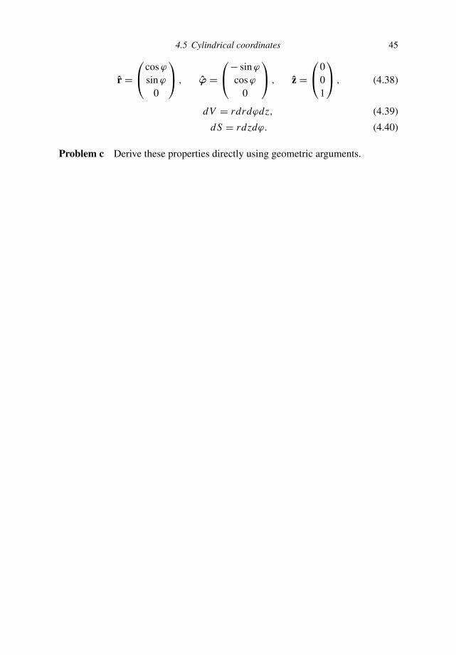
4.5 Cylindrical coordinates 45
r =⎛
⎝
cos ϕ
sin ϕ
0
⎞
⎠ , ϕ =⎛
⎝
− sin ϕ
cos ϕ
0
⎞
⎠ , z =⎛
⎝
001
⎞
⎠ , (4.38)
dV = rdrdϕdz, (4.39)
d S = rdzdϕ. (4.40)
Problem c Derive these properties directly using geometric arguments.

5
Gradient
In this chapter the gradient of a function is introduced. The gradient plays an im-portant role in the differentiation and integration of functions in more than onedimension (Section 5.3). Newton’s law is derived in Section 5.4 from the con-cept of energy conservation. As a by-product of this derivation it follows that theforce is the (negative) gradient of the potential energy. The gradient plays a cru-cial role in the distinction between the partial time derivatives and the total timederivatives. This resulting distinction between an Eulerian and a Lagrangian for-mulation of problems involving fluid flow is shown in Section 5.5. In Section 5.6expressions in spherical coordinates and cylindrical coordinates for the gradient arederived.
5.1 Properties of the gradient vector
Let us consider a function f that depends on the variables x and y in a plane. Wewant to describe how this function changes when we move from point A in theplane to point C as shown in Figure 5.1. The resulting change in the function f isdenoted by δ f = fC − f A, where f A denotes, for example, the function f at pointA. It follows from Figure 5.1 that
f A = f (x, y),fB = f (x + δx, y),fC = f (x + δx, y + δy).
⎫
⎬
⎭
(5.1)
It follows by adding and subtracting fB that
δ f = fC − f A = fB − f A + fC − fB . (5.2)
46
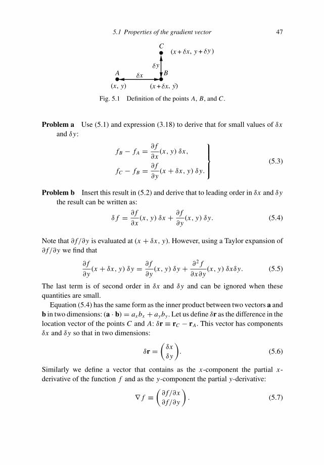
5.1 Properties of the gradient vector 47
Fig. 5.1 Definition of the points A, B, and C .
Problem a Use (5.1) and expression (3.18) to derive that for small values of δxand δy:
fB − f A = ∂ f
∂x(x, y) δx,
fC − fB = ∂ f
∂y(x + δx, y) δy.
⎫
⎪
⎪
⎬
⎪
⎪
⎭
(5.3)
Problem b Insert this result in (5.2) and derive that to leading order in δx and δythe result can be written as:
δ f = ∂ f
∂x(x, y) δx + ∂ f
∂y(x, y) δy. (5.4)
Note that ∂ f/∂y is evaluated at (x + δx, y). However, using a Taylor expansion of∂ f/∂y we find that
∂ f
∂y(x + δx, y) δy = ∂ f
∂y(x, y) δy + ∂2 f
∂x∂y(x, y) δxδy. (5.5)
The last term is of second order in δx and δy and can be ignored when thesequantities are small.
Equation (5.4) has the same form as the inner product between two vectors a andb in two dimensions: (a · b) = ax bx + ayby . Let us define δr as the difference in thelocation vector of the points C and A: δr ≡ rC − rA. This vector has componentsδx and δy so that in two dimensions:
δr =(
δxδy
)
. (5.6)
Similarly we define a vector that contains as the x-component the partial x-derivative of the function f and as the y-component the partial y-derivative:
∇ f ≡(
∂ f/∂x∂ f/∂y
)
. (5.7)

48 Gradient
This vector is called the gradient of f . It is customary to denote the gradient of afunction f by the symbol ∇ f , but another notation you may find in the literatureis grad f .
Problem c Show that the increment δ f of expression (5.4) can be expressed asthe inner product of two vectors:
δ f = (∇ f · δr). (5.8)
This expression shows directly why the gradient is such a useful vector. Oncewe know the gradient ∇ f , we can use (5.8) to compute the change in the functionf when we change the point of evaluation with an arbitrary step δr. Note that thisexpression holds for any direction in which we can take this step. It should benoted that (5.8) is based on the first order Taylor expansions in expression (5.3).This means that (5.8) only holds in the limit δr → 0. However, this expression isstill extremely useful because it forms the basis of the rules for differentiation andintegration in more than one dimension. We will return to this issue in Section 5.3.
Problem d The derivation up to this point has been for two space dimensionsonly. Repeat this derivation for three space dimensions and derive that (5.8)still holds when the gradient in three dimensions is defined as
∇ f ≡⎛
⎝
∂ f/∂x∂ f/∂y∂ f/∂z
⎞
⎠ and δr ≡⎛
⎝
δxδyδz
⎞
⎠ . (5.9)
Problem e Compute ∇ f when f (x, y, z) = x e−y sin z.
The gradient is a vector and it therefore has a direction and a magnitude. Thedirection of the gradient can be obtained from expression (5.8). Let us consider achange δr such that the function f does not change in this direction. This meansthat δr is chosen in such a way that the displacement is along a surface wheref = const . as depicted in Figure 5.2. For such a change δr, the correspondingchange δ f is by definition equal to zero, hence (∇ f · δr) = 0.
Problem f Use the properties of the inner product of two vectors to show that thisidentity implies that the vectors ∇ f and δr are for this special perturbationperpendicular: ∇ f ⊥ δr .
This last identity of course only holds when the step δr is taken along the surfacewhere the function f is constant. However, it does imply that the gradient vector is
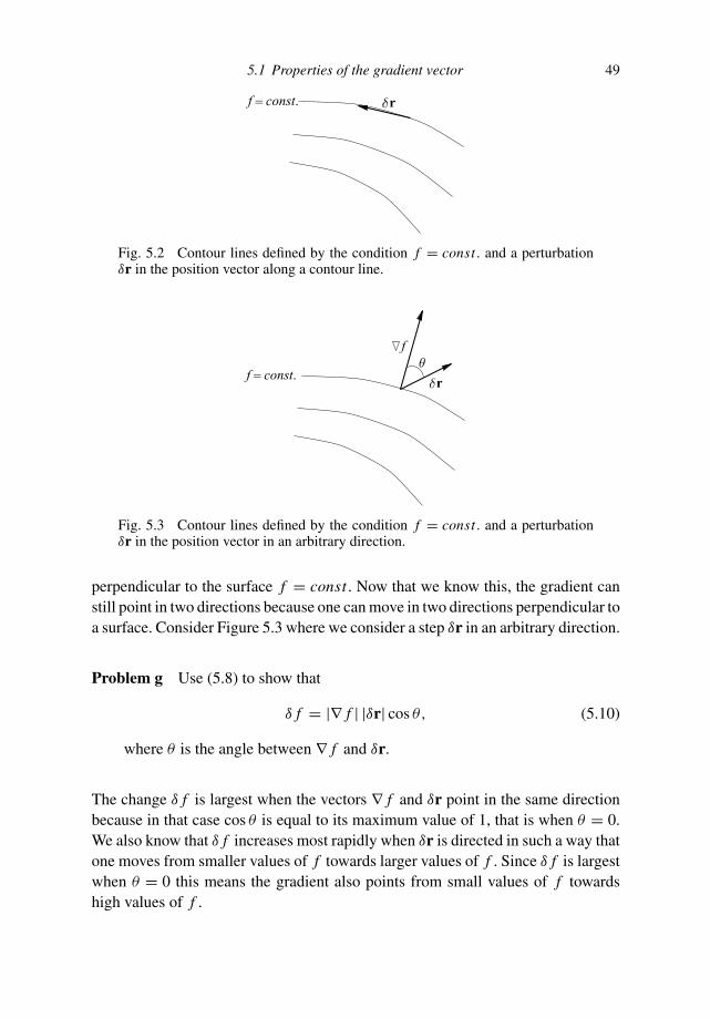
5.1 Properties of the gradient vector 49
rf const.=
Fig. 5.2 Contour lines defined by the condition f = const. and a perturbationδr in the position vector along a contour line.
rf const.
f
=
Fig. 5.3 Contour lines defined by the condition f = const. and a perturbationδr in the position vector in an arbitrary direction.
perpendicular to the surface f = const . Now that we know this, the gradient canstill point in two directions because one can move in two directions perpendicular toa surface. Consider Figure 5.3 where we consider a step δr in an arbitrary direction.
Problem g Use (5.8) to show that
δ f = |∇ f | |δr| cos θ, (5.10)
where θ is the angle between ∇ f and δr.
The change δ f is largest when the vectors ∇ f and δr point in the same directionbecause in that case cos θ is equal to its maximum value of 1, that is when θ = 0.We also know that δ f increases most rapidly when δr is directed in such a way thatone moves from smaller values of f towards larger values of f . Since δ f is largestwhen θ = 0 this means the gradient also points from small values of f towardshigh values of f .

50 Gradient
The magnitude of the gradient vector can also be obtained from (5.10). Letus consider a step δr in the direction of the gradient vector, hence a step in thedirection of increasing values of f . In that case the vectors ∇ f and δr are parallel,and cos θ = 1. This means that (5.10) implies that
|∇ f | = δ f
|δr| , (5.11)
where δr is a step in the direction of increasing values of f . Summarizing this weobtain the following properties of the gradient vector ∇ f :
1 The gradient of a function f is a vector that is perpendicular to the surface f =const .
2 The gradient points in the direction of increasing values of f .
3 The magnitude of the gradient is the change δ f in the function in the direction ofthe largest increase divided by the distance |δr| in that direction.
5.2 Pressure force
An example of a two-dimensional function is shown in Figure 5.4 where the atmo-spheric pressure on the Earth’s surface is shown in units of millibars.
Fig. 5.4 Contour map of the pressure at the Earth’s surface on 17 May 1999 inunits of millibars. (Figure courtesy of the European Centre for Medium-RangeWeather Forecasts (ECMWF).)
5.2 Pressure force 51
Problem a Draw the gradient vector of the pressure p in a number of locationson this map. When doing so draw larger arrows where the gradient is greater.
Problem b What is the approximate gradient |∇ p| over Ireland? Is the gradientvector larger over Ireland than over Iceland?
There is a good reason why a map of the pressure is used here to illustrate theconcept of the gradient. When the air pressure is not constant, a parcel of air willexperience a force that pushes it from a region of high pressure towards a regionof lower air pressure. This force increases when the pressure varies more rapidlywith distance. This can be described by the pressure force Fp that is given by:
Fp = −∇ p. (5.12)
Problem c The pressure in the weather map of Figure 5.4 is shown in units ofmillibars. If you have worked out problem b properly you will have deducedthat the units of the pressure force are in millibars per kilometre. A pressure isa force per unit area because the pressure times the area gives the total forcethat acts on this area. Deduce from this result that the pressure force has thedimensions force/volume.
Problem d Use expression (5.12) to show that the pressure force points fromregions of high pressure towards regions of lower pressure. Draw the directionof the pressure force at the high-pressure area in Figure 5.4 over Ireland.
You may have noted that we have not really derived expression (5.12) for thepressure force. Sometimes only physical arguments are used to state a physicallaw. However, one often needs to verify that the arguments employed have a propermathematical basis. It is possible to derive the pressure force from the fact thatthe force that acts in a gas or a fluid on a hypothetical surface within that mediumis perpendicular to that surface and its strength is given by the pressure times thesurface area.
Problem e Consider a small volume element with lengths δx , δy, and δz in thethree coordinate directions as shown in Figure 5.5. Let us consider the netforce in the x-direction. Use the concept of pressure as described above toshow that the force acting on the left-hand plane of the volume is given byp(x, y, z)δyδz x and that the force acting on the right-hand plane is given by−p(x + δx, y, z)δyδz x, where x is the unit vector in the x-direction. Explainthe minus sign in the second term.

52 Gradient
z
(x(x,y,z) xy
x,y,z)+Fig. 5.5 Definition of geometric variables for the derivation of the pressure force.
The top, bottom, front, and back surfaces do not contribute to the x-component ofthe pressure force because the pressure force acting on these surfaces is directed inthe y- or z-direction. This implies that the x-component of the total force is givenby
fx = −[p(x + δx, y, z) − p(x, y, z)] δyδz x. (5.13)
Problem f Use expression (3.18) to show that this can also be written as
fx = −∂p
∂xδV x, (5.14)
where the volume δV is equal to δxδyδz.
Problem g Apply the same reasoning to obtain the y- and z-com-ponents of the force and show that the net force felt by the volume is given by
f = −∇ p δV . (5.15)
You may have been puzzled by the fact that in problem c you deduced that thepressure force Fp has the dimensions f orce/volume. This means it is not reallya force. In fact, we see in (5.15) that the net force that acts on the volume isgiven by −∇ pδV . You have to keep in mind that the volume δV is not a physicalentity, instead it is a mathematical volume used in our reasoning. The net force isproportional to δV , and since this volume is physically meaningless the net forcealso has no physical meaning. However, when ρ is the mass-density of the gas orfluid then δm = ρ δV is the mass of the volume. This means that both the mass ofthe volume and the net force that acts on the volume are proportional to δV . Whenwe apply Newton’s law δma = f to this volume, we can divide both the left-hand

5.3 Differentiation and integration 53
side and the right-hand side by the arbitrary volume δV and Newton’s law thentakes the form ρa = Fp, with the pressure force given by (5.12).
This means that the pressure force Fp should be seen as a force per unit volume,just as the density ρ is the mass per unit volume. In fluid mechanics one alwaysworks with physical quantities per unit volume, for the simple reason that a gasor fluid is not composed of physical small volumes. We return to a more rigoroustreatment of Newton’s law in fluid dynamics in Section 11.3 where the conservationof momentum in a continuous medium is treated.
The pressure force is one of the most important forces in fluid mechanics, mete-orology, and oceanography because it is the variation in the pressure that underliesthe motion of fluids and gases. Physically it states the simple fact that a gas or fluidis pushed away from regions of higher pressure to regions of lower pressure.
5.3 Differentiation and integration
The results of Section 5.1 hold for infinitesimal changes δr only. However, a changeover a finite distance can be thought of as being built up from many infinitesimalsteps. Let us consider two points A and B that may be far apart as shown inFigure 5.6. Between the points A and B we can insert a large number of pointsP1, P2, . . . , PN . The difference in the function values at the points A and B canthen be written as
fB − f A = ( fB − fN ) + ( fN − fN−1) + · · · + ( f2 − f1) + ( f1 − f A) , (5.16)
where f j denotes the function evaluated at point Pj . What we are really do-ing is dividing the large distance from A to B into infinitesimally smaller inter-vals. If we take enough of these subintervals we can apply (5.8) to each of thesesub-intervals.
A PP
P B
12
N
Fig. 5.6 The definition of the points A and B at the end of an interval and theintermediary points P1, P2, . . . , PN .

54 Gradient
Problem a Show that
fB − f A =∑
(∇ f · δr), (5.17)
where the sum is over the sub-intervals used in (5.16) and where δr is theincrement in the position vector in each interval.
The analysis in this section holds only in the limit N → ∞ where the interval isdivided into infinitesimal intervals. In that case the summation in (5.17) is replacedby an integration and the notation dr is used rather than δr:
fB − f A =∫ B
A(∇ f · dr). (5.18)
This expression is extremely useful because it makes it possible to compute thechange in a function between two points once one knows the gradient of thatfunction. It should be noted that (5.18) holds for any path that joins the points Aand B. This can easily be seen from the derivation of this section, because thepoints P1, P2, . . . , PN can be arbitrarily chosen as long as they form a continuouspath that joins the points A and B. This property can sometimes be exploited bychoosing the path for which the calculation of the integral is easiest.
Problem b Use these results to show that the line integral of ∇ f along any closedcontour is equal to zero:
∮
(∇ f · dr) = 0. (5.19)
The gradient can also be used to determine the derivative of a function in a givendirection. The directional derivative d f/ds of the function in the direction of a unitvector n is defined as the change of the function in the direction of n normalizedper unit distance:
d f
ds(r) = lim
δs→0
f (r + nδs) − f (r)
δs. (5.20)
Problem c Use (5.8) in the numerator of this expression to derive that
d f
ds(r) = (n · ∇ f ) . (5.21)
This expression is important because it allows us to compute the derivative of afunction in any arbitrary direction once the gradient is known.

5.4 Newton’s law from energy conservation 55
Equations (5.18) and (5.21) generalize the rules for the integration and differen-tiation of functions of one variable to more space dimensions.
Problem d To see this, let the function f depend on the variable x only and letthe points A and B be located on the x-axis. Let x denote the unit vector inthe direction of the x-axis. Use the relation dr = xdx to show that in that case(5.18) reduces to the well-known integration rule of a function that dependsonly on one variable:
fB − f A =∫ B
A
∂ f
∂xdx . (5.22)
Problem e Let the vector n be directed along the x-axis so that n = x. Show thatin that case the directional derivative along the x-axis in (5.21) is given by∂ f/∂x .
5.4 Newton’s law from energy conservation
In classical mechanics one can start from Newton’s law and derive that the totalenergy of a mechanical system without friction is conserved. You may have discov-ered that in physics there is often no proof of the basic physical laws. For example,there is no “proof” of Newton’s law. Its use is justified by the observation that itdescribes the motion of the Sun, Moon, and planets very accurately. To a certainextent, it is arbitrary which physical law one uses as a starting point. In this sec-tion we use the concept of energy conservation as a starting point and then deriveNewton’s law.
Let us consider a mechanical system without friction. The total energy E is thesum of the kinetic energy 1
2 mv2 and the potential energy V (r):
1
2mv2 + V (r) = E . (5.23)
We assume that in such a system the total energy E is conserved; this means thatthe time derivative of this quantity is equal to zero
d E
dt= 0. (5.24)
In order to derive Newton’s law from this expression we need to take the timederivative of both the kinetic and the potential energy.

56 Gradient
Problem a Show that the time derivative of the kinetic energy is given by
d
dt
(
1
2mv2
)
= m
(
v · dvdt
)
. (5.25)
Hint: write v2 = v2x + v2
y + v2z and differentiate each term.
We also need to compute the time derivative of the potential energy. At first youmay be tempted to conclude that this time derivative is equal to zero because thepotential depends on the position r but not on time. However, as the particle movesthrough space it is at different positions at different times. Therefore, the positionof the particle is a function of time: r = r(t). For this reason, the potential shouldbe written as V (r(t)). The time derivative of the potential then follows from theusual rule for taking a derivative:
dV (r)
dt= lim
δt→0
V (r(t + δt)) − V (r(t))
δt. (5.26)
Problem b Use (5.8) to show that this time derivative can be written as
dV (r)
dt= lim
δt→0
(∇V · δr)
δt, (5.27)
with δr = r(t + δt) − r(t).
Problem c Use the definition of the velocity v = limδt→0 δr/δt to show that
dV (r)
dt= (v · ∇V ) . (5.28)
Problem d Use these results to show that the law of energy conservation (5.24)can be written as
v ·(
mdvdt
+∇V
)
= 0. (5.29)
Since v is arbitrary, (5.29) must hold for any velocity vector v. This can only be thecase when the term in brackets is equal to zero.
Problem e Show that this implies that
mdvdt
= F, (5.30)
with
F = −∇V . (5.31)
5.5 Total and partial time derivatives 57
Equation (5.30) is Newton’s law; we have derived it here from the requirementof energy conservation. As a by-product we have shown that the force in Newton’slaw is equal to −∇V . Note that the force (5.31) and the pressure force (5.12) sharethe common property that they follow from the gradient of a scalar function. Youmay find this analogy useful. We have argued in Section 5.2 that the pressure forcepushes air from a region of higher pressure to a region of lower pressure. By the samereasoning the force F = −∇V pushes a particle from regions of higher potentialenergy to regions of lower potential energy. A simple example of this is gravity.The gravitational potential energy increases with the distance to the attracting body.This means that according to the reasoning given here gravitation forces a particlecloser to the attracting body. This is an observation that may be obvious to youwhen you see an apple fall from a tree. However, you may want to keep the analogyof the pressure force and the force associated with a general potential energy inmind because it helps to understand the concept of potential energy.
With all the elements we have assembled here, we can now derive the concept ofpower. This quantity is defined as the energy delivered to the particle per unit time.This means that the power is defined as the time derivative of the kinetic energy.
Problem f Use (5.24), (5.28), and (5.31) to derive that the power is given by
d
dt
(
1
2mv2
)
= (F · v) . (5.32)
How can we understand this result? Let the particle be displaced over a distance δrin a time increment δt . The work done by the force is given by (F · δr). This meansthat the work per unit time is given by (F · δr) /δt . In the limit δt → 0 the quantityδr/δt is the velocity v, so that the power is given by (F · v) as stated in (5.32). InSection 11.3 we will derive the time derivative of the kinetic energy of a gas orfluid, and it will be shown in (11.22) that for such a system the energy delivered bythe force per unit time is also given by (F · v), with F the force per unit volume.
5.5 Total and partial time derivatives
We have seen in the previous section that the potential that acts on a particlechanges with time when the particle moves to a different location. This principleof a temporal change that is caused by a motion in the system is very general. Asan example, consider the situation in Figure 5.7 where an observer measures thetemperature in an observation tower. The motion of the wind is towards the left, anda region of warm air is transported leftward with the wind. The observer detectsan increase of the temperature with time, so that ∂T/∂t > 0. In this expression the

58 Gradient
moving left moving left
cold warm
Fig. 5.7 An observer standing on a fixed tower experiences an increase in tem-perature because warm air moves towards the observer.
cold warm
fixed fixed
v
Fig. 5.8 An observer in a balloon flies through a temperature field that is constantat each location. Because the balloon flies to a warmer region the observer detectsan increase in temperature.
partial derivative symbol is used deliberately. In general, the temperature field is afunction of both time and the space coordinates: T = T (r, t). For the observer inthe observation tower the space coordinates are fixed, which means that any changedetected by the observer is due to the temporal change of the local temperatureonly, but that the location is fixed. This is expressed by the definition of the partialderivative:
∂T (r, t)
∂t≡ lim
δt→0
T (r,t + δt) − T (r, t)
δt. (5.33)
In this derivative the time is varied but all other variables are kept fixed.In contrast to the previous example let us now consider an observer that is carried
along in a balloon by the wind, see Figure 5.8. We assume in this situation that the

5.5 Total and partial time derivatives 59
temperature field is fixed in time, so that ∂T/∂t = 0. The observer is carried by thewind from a cold region to a warmer region. This means that just like the observerin Figure 5.7 this second observer experiences an increase in the temperature. Therate of change of the temperature is denoted by the total time derivative dT/dt . Wecan see from this example that dT/dt can be larger than zero while ∂T/∂t = 0.The total time derivative is defined in the following way:
dT (r, t)
dt= lim
δt→0
T (r(t + δ),t + δt) − T (r(t), t)
δt. (5.34)
The only difference between this and the partial time derivative (5.33) is that in(5.34) the position of the observation point changes, whereas in the partial timederivative (5.33) the position is fixed.
Problem a Assuming that the temperature field in Figure 5.8 depends on positionbut not on time, show that dT/dt has the same form as expression (5.26) anduse the results of Section 5.4 to show that for the observer in Figure 5.8
dT (r)
dt= (v · ∇T ) (in the special case of Figure 5.8). (5.35)
Problem b Draw the gradient vector ∇T in Figure 5.8 at the location of theobserver and show from the geometry of this vector and the velocity vectorthat dT/dt > 0.
This means that both observers in Figures 5.7 and 5.8 detect a rise in temperature,but their description of this temperature change is completely different. The firstobserver feels an increase in temperature because the local temperature changes atthat observer’s location; this is described by the partial time derivative ∂T/∂t . Thesecond observer detects an increase in temperature because that second observer istransported to a warmer region in a fixed temperature field; this is describes by thetotal time derivative that is for this special case given by dT/dt = (v · ∇T ).
In general the temperature field may change because of a combination of achange in the temperature at a fixed location and a movement of the observer. Wewill assume now that the temperature field depends on all three space coordinatesand on time: T = T (x(t), y(t), z(t), t). In this notation it is explicit that the spacecoordinates of the observation point depend on time as well. The total time derivativeis given by (5.34) and can be written as:
dT
dt= lim
δt→0
T (x(t + δt), y(t + δt), z(t + δt), t + δt) − T (x(t), y(t), z(t), t)
δt.
(5.36)
60 Gradient
Let the x-coordinate over the time interval change from x to x + δx , and the y- andz-coordinates change in a similar way.
Problem c Use the first order Taylor series to show that
δx = x(t + δt) − x(t) ≈ ∂x
∂tδt = vxδt. (5.37)
In the limit δt → 0 the approximation becomes an identity. Explain that vx isthe x-component of the velocity vector.
Problem d Generalize (3.22) for the case of a function that depends both on x ,y, z, and on t to the following first order Taylor series:
T (x + δx, y + δy, z + δz, t + δt) ≈ T (z, y, z, t)
+ ∂T
∂xδx + ∂T
∂yδy + ∂T
∂zδz + ∂T
∂tδt. (5.38)
Problem e Insert (5.37) and (5.38) in (5.36) and take the limit δt → 0 to derivethat
dT
dt= ∂T
∂xvx + ∂T
∂yvy + ∂T
∂zvz + ∂T
∂t. (5.39)
Problem f Use the definition of the gradient vector to rewrite this as
dT
dt= ∂T
∂t+ (v · ∇T ) . (5.40)
Problem g This is the general expression of the total time derivative. Show thatthe time derivatives (5.33) and (5.35) seen by the observers in Figures 5.7and 5.8 can both be obtained from this general expression for the total timederivative.
The temperature field was used in this section only for illustrative purposes.The analysis is of course applicable to any function that depends on both timeand the space coordinates. Also, in the analysis we used “observers” to fix ourminds. However, in general there are no observers and it is not essential that thereis anybody present to “observe” the change in temperature. The total time derivativeis always related to the movement of a certain quantity. In Section 5.4 this was themovement of a particle that is subjected to a potential V (r). In the description ofa gas it may concern the motion of a parcel of material in the gas that is carriedaround by the flow.
5.6 Gradient in spherical coordinates 61
Whenever one describes a continuous system such as the motion in the atmo-sphere one has a choice in the way that one sets up this description. One optionis to consider every quantity at a fixed location in space, and to specify how thesequantities change with time. In that case the change of the properties with time isdescribed by the partial time derivative ∂/∂t . This is called an Eulerian description.As an alternative one may follow a certain property while it is being carried aroundby the flow. In that case the change of this property with time is given by the totaltime derivative d/dt . This is called a Lagrangian description. Which descriptionis most convenient depends on the problem. In numerical applications the Euleriandescription is usually most convenient because one can work with a fixed systemof space coordinates and one only needs to specify how a property changes withtime in that coordinate system. On the other hand, if one wants to study, for ex-ample, the spreading of pollution by wind one aims at tracking particles, and forthis the Lagrangian formulation is most convenient. For this reason it is importantthat one can transform the physical laws back and forth between an Eulerian and aLagrangian formulation. We return to this issue in Chapter 11.
5.6 Gradient in spherical coordinates
The gradient vector is defined in (5.9) using a system of Cartesian coordinates. Inmany applications it is much more convenient to use a system of curvilinear coor-dinates, especially spherical coordinates and cylindrical coordinates. It is thereforeuseful to obtain the form of the gradient in these coordinate systems as well. In thissection we consider the expression of the gradient in spherical coordinates. Beforewe do this we first rewrite the expression of the gradient in Cartesian coordinates.
Problem a Show that the gradient in Cartesian coordinates can also be writtenas:
∇ f = x∂ f
∂x+ y
∂ f
∂y+ z
∂ f
∂z. (5.41)
Problem b Take the inner product of this expression with the unit vector in thex-direction to show that
∂ f
∂x= (x · ∇ f ) . (5.42)
Expression (4.4) gives the spherical coordinates r , θ , and ϕ in terms of theCartesian coordinates x , y, and z. Using the chain rule of differentiation one can

62 Gradient
then use for example that
∂
∂x= ∂r
∂x
∂
∂r+ ∂θ
∂x
∂
∂θ+ ∂ϕ
∂x
∂
∂ϕ.
Together with expression (4.7) for the unit vectors r, θ, and ϕ this could be usedto derive the expression for the gradient in spherical coordinates. However, this ap-proach is algebraically very complex and does not give much insight. Here we derivethe gradient vector in spherical coordinates using (5.8). The idea is that the com-ponent of the gradient along a certain coordinate axis is simply given by the rate ofchange of the function in that direction: δ f = (∇ f · δs). Suppose that the change inposition δs is in the direction of a unit vector e, then the change in position is givenby δs = e δs, where δs is given by: δs ≡ |δs|. This means that δ f = (∇ f · e) δs.However, as (∇ f · e) is the component of the gradient vector in the direction ofthe unit vector e, this means that the component ∇e f of the gradient vector in thedirection of e is given by:
∇e f ≡ (∇ f · e) = δ f
δs= lim
δs→0
f (r + eδs) − f (r)
δs. (5.43)
Consider the spherical coordinate system shown in Figure 5.9. Let us move in thedirection of the unit vector θ from the point A with spherical coordinates (r, θ, ϕ)to point B with spherical coordinates (r, θ + δθ, ϕ).
Problem c Derive from Figure 5.9 that the distance δs between the points A andB is related to the change in the angle δθ by the relation δs = rδθ .
B
A
r
D C
r
Fig. 5.9 Definition of the geometric variables and the points A, B, C , and D inspherical coordinates.
5.6 Gradient in spherical coordinates 63
Problem d Use this in (5.43) to derive that the θ -component of the gradient vectoris given by
∇θ f = limδθ→0
f (r, θ + δθ, ϕ) − f (r, θ, ϕ)
rδθ= 1
r
∂ f
∂θ. (5.44)
Problem e For a change from point A to point C in the r direction over anincrement δr in the radius the change in the position has magnitude δs = δr .Derive from this that the radial component is given by
∇r f = ∂ f
∂r. (5.45)
Problem f Use the geometry of Figure 5.9 to show that for a change from pointA to point D in the ϕ-direction over an increment δϕ in the azimuth ϕ thechange in the position has magnitude δs = r sin θ δϕ. Derive from this thatthe azimuthal component of the gradient is given by
∇ϕ f = 1
r sin θ
∂ f
∂ϕ. (5.46)
Combining these results we obtain the expression for the gradient in sphericalcoordinates:
∇ f = r∂ f
∂r+ θ
1
r
∂ f
∂θ+ ϕ
1
r sin θ
∂ f
∂ϕ. (5.47)
Note that the gradient in spherical coordinates is not given by ∇ f = r∂ f/∂r +θ∂ f/∂θ + ϕ∂ f/∂ϕ. There is a simple reason why this expression must be wrong.The first term on the right-hand side has the dimension f/ length because theradius is a length, while the second term has the dimension f because the angleθ is expressed in radians which is a dimensionless property. This means that thisexpression must be wrong. The factors 1/r and 1/r sin θ in (5.47) account for thescaling of the distance δs with the change in the angles δθ and δϕ, respectively.These terms therefore account for the fact that the system is curvilinear.
Problem g Show that each of the terms in (5.47) has the dimension f/ length.
Problem h Do the same analysis for cylindrical coordinates and show that thegradient in cylindrical coordinates is given by
∇ f = r∂ f
∂r+ ϕ
1
r
∂ f
∂ϕ+ z
∂ f
∂z. (5.48)
6
Divergence of a vector field
The physical meaning of the divergence cannot be understood without understand-ing what the flux of a vector field is, and what the sources and sinks of a vectorfield are.
6.1 Flux of a vector field
To fix our mind, let us consider a vector field v(r) that represents the flow of a fluidthat has a constant density. We define a surface S in this fluid. Of course the surfacehas an orientation in space, and the unit vector perpendicular to S is denoted by n.Infinitesimal elements of this surface are denoted with dS ≡ nd S. Now supposewe are interested in the volume of fluid that flows per unit time through the surfaceS; this quantity is called Φ. When we want to know the flow through the surface,we only need to consider the component of v perpendicular to the surface, the flowalong the surface is not relevant.
Problem a Show that the component of the flow across the surface is given by(v · n)n and that the flow along the surface is given by v − (v · n)n. If you findthis problem difficult you may want to look ahead to Section 13.1.
Using this result the volume of the flow through the surface per unit time is givenby:
Φv =∫∫
(v · n) d S =∫∫
v · dS; (6.1)
this expression defines the flux Φv of the vector field v through the surface S. Thedefinition of a flux is not restricted to the flow of fluids: a flux can be computed forany vector field. However, the analogy of fluid flow often is useful for understandingthe meaning of the flux and divergence.
64
6.1 Flux of a vector field 65
The electric field generated by a point charge q at the origin is given by
E(r) = q r4πε0r2
. (6.2)
In this expression r is the unit vector in the radial direction and ε0 is the permittivity.A surface element on a sphere of radius R is given by d S = R2dΩ, with dΩ =sin θdθdϕ an increment in the solid angle on the unit sphere. The normal to thespherical surface is given by r, so that the oriented surface element is given bydS = rR2dΩ.
Problem b Show that the flux of the electric field through a spherical surface ofradius R with the point charge at its center is given by
ΦE =∫∫
E · dS = q
4πε0 R2
∫∫
(r · r) R2dΩ = q
4πε0
∫ 2π
0
∫ π
0sin θdθdϕ.
(6.3)The last identity implies that this flux is independent of the radius R.
Problem c Carry out the integration over the angles to show that the flux is givenby
ΦE = q
ε0. (6.4)
This means that the flux depends on the charge q and the permittivity ε0, but noton the radius of the surface.
As a next example we compute the flux of the magnetic field of the Earth throughthe Earth’s surface. The radius of the Earth is denoted by R. To first order themagnetic field of the Earth is a dipole field. (This is the field generated by a magneticnorth pole and magnetic south pole that are very close together.) The dipole vectorm points from the south pole of the dipole to the north pole and its size is givenby the strength of the dipole. The magnetic field B(r) is given by (reference [53],p. 182):
B(r) = 3r(r · m) − mr3
. (6.5)
We are free to choose the orientation of the coordinate axes. Let us align thez-axis of the coordinate system by the dipole vector, in that case m = mz,and
B(r) = m3r(r · z) − z
r3. (6.6)

66 Divergence of a vector field
Problem d According to Figure 4.1, (r · z) = cos θ . Use this result and the rela-tion dS = rR2 sin θdθdϕ to show that the magnetic flux is given by
ΦB = m∫ 2π
0
∫ π
0
3 cos θ − cos θ
R3R2 sin θdθdϕ. (6.7)
Problem e Carry out the integration over the angle θ to show that this flux van-ishes.
This means that the total magnetic flux through the surface of the Earth vanishes.Physically this implies that as many magnetic field lines point out of the Earth asinto the Earth. The electric field of a positive charge points away from the charge.As shown in expression (6.4) this gives a nonzero flux of the electric field througha spherical surface around that charge. This situation is different for the magneticfield where field lines point away from the dipole as well as towards the dipole,which causes the magnetic flux to vanish.
6.2 Introduction of the divergence
In order to introduce the divergence, consider an infinitesimal rectangular volumewith sides dx , dy, and dz (see Figure 6.1 for the definition of the geometric vari-ables). The outward flux through the right surface perpendicular through the x-axisis given by vx (x + dx, y, z)dydz, because vx (x + dx, y, z) is the component of theflow perpendicular to that surface and dydz is the area of the surface. By the sametoken, the flux through the left surface perpendicular through the x-axis is given by
xdz
dy
dx
Fig. 6.1 Definition of the geometric variables in the calculation of the flux of avector field through an infinitesimal rectangular volume.

6.2 Introduction of the divergence 67
−vx (x, y, z)dydz, the minus sign is due to the fact that the component of v in thedirection outward from the cube is given by −vx . (Alternatively one can say thatfor this surface the unit vector perpendicular to the surface and pointing outwards isgiven by n = −x.) This means that the total outward flux through the two surfaces isgiven by vx (x + dx, y, z)dydz − vx (x, y, z)dydz = (∂vx/∂x) dxdydz. The samereasoning applies to the surfaces perpendicular to the y- and z-axes. This meansthat the total outward flux through the sides of the cubes is:
dΦv =(
∂vx
∂x+ ∂vy
∂y+ ∂vz
∂z
)
dV = (∇ · v) dV, (6.8)
where dV is the volume dxdydz of the cube and (∇ · v) is the divergence of thevector field v. The above definition does not really tell us yet what the divergencereally is. Dividing (6.8) by dV one obtains (∇ · v) = dΦv/dV . This allows us tostate in words what the divergence is:
The divergence of a vector field is the outward flux of the vector field perunit volume.
To fix our minds again let us consider a physical example in two dimensionsin which a fluid is pumped into this two-dimensional space at the origin r = 0.For simplicity we assume that the fluid is incompressible, which means that themass-density is constant. We do not know yet what the resulting flow field is, butwe know two things. Away from the source at r = 0 there are no sources or sinksof fluid flow. This means that the flux of the flow through any closed surface S thatdoes not enclose any sources or sinks must be zero: “what goes in must come out.”This in turn means that the divergence of the flow is zero, except possibly near thesource at r = 0:
(∇ · v) = 0 for r = 0. (6.9)
In addition we know that due to the symmetry of the problem the flow is directedin the radial direction and depends on the radius r only:
v(r) = f (r )r. (6.10)
This is enough information to determine the flow field. Of course, it is a problemthat we cannot immediately insert (6.10) in (6.9) because we have not yet derived anexpression for the divergence in cylindrical coordinates. However, there is anotherway to determine the flow from the expression above.
Problem a Use the identity r =√
x2 + y2 to show that
∂r
∂x= x
r, (6.11)

68 Divergence of a vector field
and derive the corresponding equation for y. Using expressions (6.10), (6.11),and the chain rule for differentiation show that
(∇ · v) = 2 f (r ) + rd f
dr(cylindrical coordinates) . (6.12)
Problem b Insert this result in (6.9) and show that the flow field is given byv(r) = Ar/r2. Make a sketch of the flow field.
The constant A is yet to be determined. Let a volume of liquid V be injected perunit time at the source r = 0. (Following an often used convention, the dot denotesa time derivative.)
Problem c Show that V = ∫
v · dS (where the integration is over an arbitrarysurface around the source at r = 0). Choosing a suitable surface, derive that
v(r) = V
2π
rr. (6.13)
Note that the unit vector r is now used rather than the position vector r. Thesevectors are related by the expression r = r r.
From this simple example of a single source at r = 0 more complex examplescan be obtained. Suppose we have a source at r+ = (L , 0), where a volume V isinjected per unit time, and a sink at r− = (−L , 0), where a volume −V is removedper unit time. The total flow field can be obtained by superposition of flow fieldsof the form (6.13) for the source and the sink. The flow field from the source at r+can be found by replacing the location vector r in (6.13) by the vector r − r+. Thisamounts to the following replacements:
r =√
x2 + y2 →√
(x − L)2 + y2, (6.14)
and
r = r/r =(
xy
)
/√
x2 + y2 →(
x − Ly
)
/
√
(x − L)2 + y2. (6.15)
Problem d Make similar replacements for the sink at r− and show that the x- andy-components of the flow field in this case are given by:
vx (x, y) = V
2π
[
x − L
(x − L)2 + y2− x + L
(x + L)2 + y2
]
, (6.16)
vy(x, y) = V
2π
[
y
(x − L)2 + y2− y
(x + L)2 + y2
]
, (6.17)

6.3 Sources and sinks 69
and sketch the resulting flow field. This is most easily accomplished by de-termining from these expressions the flow field at some selected lines such asthe x- and y-axes.
One may also be interested in computing the streamlines of the flow. These are thelines along which material particles flow. The streamlines can be found by usingthat the time derivative of the position of a material particle is the velocity:
dr/dt = v(r). (6.18)
Inserting expressions (6.16) and (6.17) into equation (6.18) leads to two coupleddifferential equations for x(t) and y(t) which are difficult to solve. Fortunately,there are more intelligent ways of retrieving the streamlines. We return to this issuein Section 16.3.
6.3 Sources and sinks
In the above example, the fluid flow moves away from the source and convergeson the sink. The terms “source” and “sink” have a clear physical meaning sincethey are directly related to the “source” of water as from a tap, and a “sink” as thesink in a bathtub. The flow lines of the water flow diverge from the source whilethey converge towards the sink. This explains the term “divergence”, because thisquantity simply indicates to what extent flow lines originate (in the case of a source)or end (in the case of a sink).
This definition of sources and sinks is not restricted to fluid flow. For example, forthe electric field the term “fluid flow” should be replaced by the term “field lines.”Electrical field lines originate at positive charges and end at negative charges. Wefirst verify this by computing the divergence of the electrical field (6.2) for a pointcharge in three dimensions.
Problem a Show that expression (6.2) can be written as
E(r) = q
4πε0r3
⎛
⎝
xyz
⎞
⎠ . (6.19)
Problem b The x-derivative of the x-component of the electric field gives a con-tribution
∂
∂x
x
r3= 1
r3− 3x
r4
∂r
∂x. (6.20)

70 Divergence of a vector field
Use expression (6.11) to show that this quantity is given by
∂
∂x
x
r3= 1
r5
(
r2 − 3x2)
. (6.21)
Problem c Compute the y, and z-derivatives in the divergence of the electric fieldas well and show that
(∇ · E) = q
4πε0r5
(
3r3 − 3(x2 + y2 + z2)) = 0. (6.22)
This means that away from the point charge (r = 0) the divergence of the electriccharge vanishes. At the charge, r = 0 and it is not clear what the right-hand sideof expression (6.22) is. It follows from equation (6.4) that the net flux througha spherical surface is given by q/ε0. This flux is nonzero when the charge q isnonzero. For a positive charge the flux is positive, while for a negative charge theflux is negative. According to expression (6.22) the divergence vanishes for r = 0.The flux can be nonzero only when the divergence is nonzero at the location of thepoint charge.
Physically this means that the electric charge is the source of the electric field.This is reflected in the Maxwell equation for the divergence of the electric field:
(∇ · E) = ρ(r)/ε0. (6.23)
In this expression ρ(r) is the charge density, which is simply the electric charge perunit volume just as the mass-density denotes the mass per unit volume. In addition,expression (6.23) contains the permittivity ε0. This term serves as a coupling con-stant since it describes how “much” electrical field is generated by a given electricalcharge density. It is obvious that a constant is needed here because the charge densityand the electrical field have different physical dimensions, hence a proportionalityfactor must be present. However, the physical meaning of a coupling constant goesmuch deeper, because it prescribes how strong the field is that is generated by agiven source. This constant describes how strongly cause (the source) and effect(the field) are coupled.
As the next example we compute the divergence of the magnetic field (6.5)generated by a dipole m. We are free to choose the orientation of the coordinatesystem. In the following we choose the z-axis to be aligned with the dipole vectorm, this means that m = mz.
Problem d Use this expression and the relation r = r/r to show that the magneticfield (6.5) can be written as
B = 3mr (r · z)
r5− mz
r3. (6.24)
6.4 Divergence in cylindrical coordinates 71
Problem e Write the vectors r and z in component form to show that the compo-nents of the magnetic field are given by
B =⎛
⎝
3mxz/r5
3myz/r5
3mz2/r5 − m/r3
⎞
⎠ . (6.25)
Problem f Differentiate the different components to show that
∂ Bx
∂x= 3m
(
z
r5− 5x2z
r7
)
,
∂ By
∂y= 3m
(
z
r5− 5y2z
r7
)
,
∂ Bz
∂z= 3m
(
3z
r5− 5z3
r7
)
.
(6.26)
Problem g Add these terms to show that the divergence of the magnetic fieldvanishes:
(∇ · B) = 0. (6.27)
By analogy with (6.23) one might expect that the divergence of the magneticfield is nonzero at the source of the field and that it is related to a magnetic chargedensity:
(∇ · B) = coupling const. × ρB(r),
where ρB would be the “density of magnetic charge.” However, particles with amagnetic charge (usually called “magnetic monopoles”) have not been found in na-ture despite extensive searches. Therefore the Maxwell equation for the divergenceof the magnetic field is:
(∇ · B) = 0, (6.28)
but we should remember that this divergence is zero because of the observationalabsence of magnetic monopoles rather than a vanishing coupling constant.
6.4 Divergence in cylindrical coordinates
In the previous analysis we have expressed the divergence in Cartesian coordinates:∇ · v = ∂xvx + ∂yvy + ∂zvz . As you may have discovered, the use of other coordi-nate systems such as cylindrical coordinates or spherical coordinates can often make

72 Divergence of a vector field
d
vr
r
.
dr
dz
Fig. 6.2 Definition of the geometric variables for the computation of the diver-gence in cylindrical coordinates.
life much simpler. Here we derive an expression for the divergence in cylindricalcoordinates. In this system, the distance r =
√
x2 + y2 of a point to the z-axis, theazimuth ϕ(= arctan(y/x)) and z are used as coordinates, see Section 4.5. A vectorv can be decomposed into components in this coordinate system:
v = vr r + vϕϕ + vz z, (6.29)
where r, ϕ, and z are unit vectors in the direction of increasing values of r , ϕ, andz, respectively. As shown in Section 6.2 the divergence is the flux per unit volume.Let us consider the infinitesimal volume corresponding to increments dr , dϕ, anddz shown in Figure 6.2. Let us first consider the flux of v through the surfaceelements perpendicular to r. The size of this surface is rdϕdz and (r + dr )dϕdzat r and r + dr respectively. The normal components of v through these surfacesare vr (r, ϕ, z) and vr (r + dr, ϕ, z) respectively. Hence the total flux through thesetwo surface is given by vr (r + dr, ϕ, z)(r + dr )dϕdz − vr (r, ϕ, z)(r )dϕdz.
Problem a Show that to first order in dr this quantity is equal to
∂
∂r(rvr ) drdϕdz.
Hint: use a first order Taylor expansion for vr (r + dr, ϕ, z) in the quantity dr .
Problem b Show that the flux through the surfaces perpendicular to ϕ is to firstorder in dϕ given by (∂vϕ/∂ϕ)drdϕdz.
Problem c Show that the flux through the surfaces perpendicular to z is to firstorder in dz given by (∂vz/∂z)rdrdϕdz.

6.5 Is life possible in a five-dimensional world? 73
Problem d Use Figure 6.2 to show that the volume dV is given by
dV = rdrdϕdz. (6.30)
Problem e Use the fact that the divergence is the flux per unit volume, and theresults of the previous problems to show that in cylindrical coordinates:
(∇ · v) = 1
r
∂
∂r(rvr ) + 1
r
∂vϕ
∂ϕ+ ∂vz
∂z. (6.31)
Problem f Use this result to re-derive (6.12) without using Cartesian coordinatesas an intermediary. Make sure not to confuse r with r.
In spherical coordinates a vector v can be expanded into the components vr ,vθ , and vϕ in the directions of increasing values of r , θ , and ϕ respectively. Inthis coordinate system r has a different meaning to that in cylindrical coordinatesbecause in spherical coordinates r =
√
x2 + y2 + z2.
Problem g Use the same reasoning as for the cylindrical coordinates to show thatin spherical coordinates
∇ · v = 1
r2
∂
∂r
(
r2vr) + 1
r sin θ
∂
∂θ(sin θ vθ ) + 1
r sin θ
∂vϕ
∂ϕ. (6.32)
6.5 Is life possible in a five-dimensional world?
In this section we investigate whether the motion of the Earth around the Sun isstable or not. This means that we ask ourselves whether, when the position of theEarth is perturbed (for example by the gravitational attraction of the other planetsor by a passing asteroid), the gravitational force causes the Earth to return to itsoriginal position (stability) or to spiral away from (or towards) the Sun. It turns outthat these stability properties depend on the spatial dimension! We know that welive in a world of three spatial dimensions, but it is interesting to investigate whetherthe orbit of the Earth would also be stable in a world with a different number ofspatial dimensions.
In the Newtonian theory the gravitational field g(r) satisfies (see reference [76]):
(∇ · g) = −4πGρ, (6.33)
where ρ(r) is the mass-density and G is the gravitational constant which has a valueof 6.67 × 10⁻⁸ cm3 g−1 s−2. The term G plays the role of a coupling constant, justlike the 1/permittivity in (6.23). Note that the right-hand side of the gravitational

74 Divergence of a vector field
field equation (6.33) has the opposite sign to the right-hand side of the electricfield equation (6.23). This is due to the fact that two electric charges of equal signrepel each other, while two masses of equal sign (mass being positive) attract eachother. Zee [125] gives an insightful explanation based on quantum field theory ofthis fundamental difference between the electrical field and the gravitational field.If the sign of the right-hand side of (6.33) was positive, masses would repel eachother and structures such as planets, the solar system, and stellar systems wouldnot exist.
Problem a We argued in Section 6.3 that electric field lines start at positivecharges and end at negative charges. By analogy we expect that gravitationalfield lines end at the (positive) masses that generate the field. However, wheredo the gravitational field lines start?
Let us first determine the gravitational field of the Sun in N dimensions. Outsidethe Sun the mass-density vanishes; this means that (∇ · g) = 0. We assume that themass-density in the Sun is spherically symmetric, then the gravitational field mustalso be spherically symmetric and is thus of the form:
g(r) = f (r )r. (6.34)
In order to make further progress we must derive the divergence of a sphericallysymmetric vector field in N dimensions. Generalizing expression (6.32) to an ar-bitrary number of dimensions is not trivial, but fortunately this is not needed. We
will make use of the property that in N dimensions: r =√
∑Ni=1 x2
i .
Problem b Derive from this expression that
∂r/∂x j = x j/r. (6.35)
Use this result to derive that for a vector field of the form (6.34):
(∇ · g) = N f (r ) + r∂ f
∂r. (6.36)
Outside the Sun, where the mass-density vanishes and (∇ · g) = 0 we can use thisresult to determine the gravitational field.
Problem c Derive that
g(r) = − A
r N−1r, (6.37)
and check this result for three spatial dimensions.

6.5 Is life possible in a five-dimensional world? 75
At this point the constant A is not determined, but this is not important for the comingarguments. The minus sign has been added for convenience: the gravitational fieldpoints towards the Sun and hence A > 0.
Associated with the gravitational field is a gravitational force that attracts theEarth towards the Sun. If the mass of the Earth is denoted by m, this force is givenby
Fgrav = − Am
r N−1r, (6.38)
and is directed towards the Sun. For simplicity we assume that the Earth is in acircular orbit. This means that the attractive gravitational force is balanced by therepulsive centrifugal force which is given by
Fcent = mv2
rr. (6.39)
In equilibrium these forces balance: Fgrav + Fcent = 0.
Problem d Derive the velocity v from this requirement.
We now assume that the distance to the Sun changes from r to r + δr ; theperturbation in the position is therefore δr = δr r. Because of this perturbation, thegravitational force and the centrifugal force are also perturbed. These quantitieswill be denoted by δFgrav and δFcent respectively, see Figure 6.3. The change in thetotal force is given by δFgrav + δFcent . Let us first suppose that the Earth movesaway from the Sun, in that case δr point from the Sun to the Earth. The orbit isstable when the net perturbation of the force draws the Earth back towards the Sun.In that case the vectors δr and
(
δFgrav + δFcent)
point in opposite directions and(
δFgrav + δFcent
) · δr < 0 (stability). (6.40)
Suppose on the other hand that the Earth moves towards the Sun, in that case δrpoints towards the Sun. The orbit is stable when the perturbation of the force pushesthe Earth away from Sun. In that case the vectors δr and
(
δFgrav + δFcent
)
point inopposite directions as well so that (6.40) is satisfied. This means that the orbitalmotion is stable for perturbations when the gravitational field satisfies the criterion(6.40).
In order to compute the change in the centrifugal force we use that angularmomentum is conserved, that is
mrv = m(r + δr )(v + δv). (6.41)
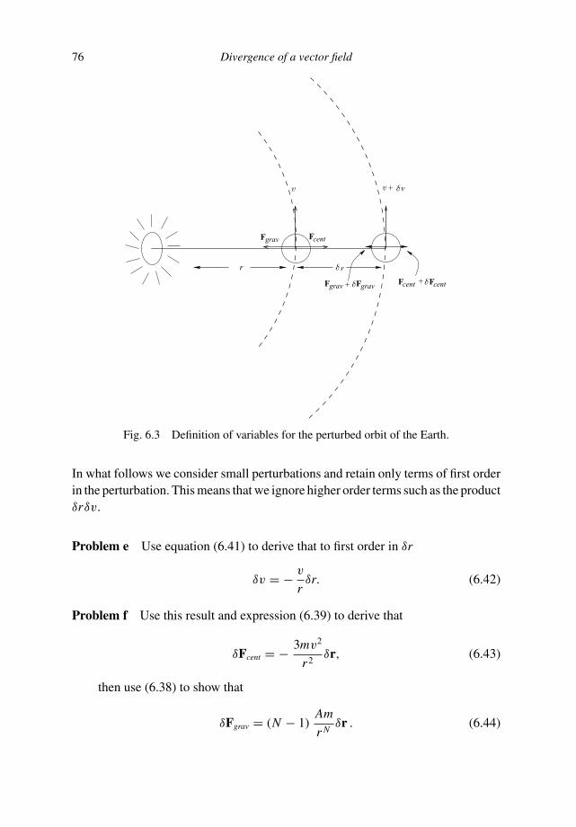
76 Divergence of a vector field
rr
+ v
grav cent
++grav
F F
gravFF centcent FF
Fig. 6.3 Definition of variables for the perturbed orbit of the Earth.
In what follows we consider small perturbations and retain only terms of first orderin the perturbation. This means that we ignore higher order terms such as the productδrδv.
Problem e Use equation (6.41) to derive that to first order in δr
δv = − v
rδr. (6.42)
Problem f Use this result and expression (6.39) to derive that
δFcent = − 3mv2
r2δr, (6.43)
then use (6.38) to show that
δFgrav = (N − 1)Am
r Nδr . (6.44)

6.5 Is life possible in a five-dimensional world? 77
Note that the perturbation of the centrifugal force does not depend on the number ofspatial dimensions, but that the perturbation of the gravitational force does dependon N .
Problem g Use the value of the velocity derived in problem d and expressions(6.43)–(6.44) to show that according to the criterion (6.40) the orbital motionis stable in less than four spatial dimensions. Show also that the requirementfor stability is independent of the original distance r .
This is an intriguing result. It implies that orbital motion is unstable in more thanfour spatial dimensions. This means that in a world with five spatial dimensions thesolar system would not be stable. Life seems to be tied to planetary systems with acentral star which supplies the energy to sustain life on the orbiting planet(s). Thisimplies that life would be impossible in a five-dimensional world! Note also that thestability requirement is independent of r , that is the stability properties of orbitalmotion do not depend on the size of the orbit. This implies that the gravitationalfield does not have “stable regions” and “unstable regions”, the stability propertydepends only on the number of spatial dimensions.

7
Curl of a vector field
7.1 Introduction of the curl
We introduce the curl of a vector field v by its formal definition in terms of Cartesiancoordinates (x, y, z) and unit vectors x, y, and z in the x-, y-, and z-directionsrespectively:
curl v ≡∣
∣
∣
∣
∣
∣
x y z∂x ∂y ∂z
vx vy vz
∣
∣
∣
∣
∣
∣
=⎛
⎝
∂yvz − ∂zvy
∂zvx − ∂xvz
∂xvy − ∂yvx
⎞
⎠ . (7.1)
It can be seen that the curl is a vector, in contrast to the divergence which is a scalar.The notation with the determinant is sloppy because the entries in a determinantshould be numbers rather than vectors such as x or differentiation operators suchas ∂y = ∂/∂y. However, the notation in terms of a determinant is a simple way toremember the definition of the curl in Cartesian coordinates. We will write the curlof a vector field also as: curl v = ∇ × v.
Problem a Verify that this notation with the curl expressed as the outer productof the operator ∇ and the vector v is consistent with definition (7.1).
In general the curl is a three-dimensional vector. To see the physical interpretationof the curl, we will make life easy for ourselves by choosing a Cartesian coordinatesystem in which the z-axis is aligned with curl v. In that coordinate system the curlis given by: curl v = (∂xvy − ∂yvx )z. Consider a little rectangular surface elementoriented perpendicular to the z-axis with sides dx and dy respectively, see Fig-ure 7.1. We consider the line integral
∮
dxdy v · dr along a closed loop defined by thesides of this surface element, integrating in the counterclockwise direction. Thisline integral can be written as the sum of the integral over the four sides of thesurface element.
78

7.1 Introduction of the curl 79
x
dx
dy
y
y + dy
x + dx
Fig. 7.1 Definition of the geometric variables for the interpretation of the curl.
Problem b Show that the line integral is given by∮
dxdy v · dr = vx (x, y)dx +vy(x + dx, y)dy − vx (x, y + dy)dx − vy(x, y)dy, and use a first order Taylorexpansion to write this as
∮
dxdyv · dr = (∂xvy − ∂yvx ) dxdy, (7.2)
with vx and vy evaluated at the point (x, y).
This expression can be rewritten as:
(curl v)z = (∂xvy − ∂yvx ) =∮
dxdy v · dr
dxdy. (7.3)
In this form we can express the meaning of the curl in words:
The component of curl v in a certain direction is the closed line integralof v along a closed path perpendicular to this direction, normalized perunit surface area.
Note that this interpretation is similar to the interpretation of the divergence givenin Section 6.2. There is, however, one major difference. The curl is a vector whilethe divergence is a scalar. This is reflected in our interpretation of the curl becausea surface has an orientation defined by its normal vector, hence the curl is also avector.

80 Curl of a vector field
7.2 What is the curl of the vector field?
In order to discover the meaning of the curl, we consider again an incompressiblefluid and study the curl of the velocity vector v, because this will allow us todiscover the physical meaning of the curl. It is not only for a didactic purpose thatwe consider the curl of fluid flow. In fluid mechanics this quantity plays such acrucial role that it is given a special name, the vorticity ω:
ω ≡ ∇ × v. (7.4)
To simplify things further we assume that the fluid moves in the (x, y)-plane only(i.e. vz = 0) and that the flow depends only on x and y: v = v(x, y).
Problem a Show that for such a flow
ω = ∇ × v = (∂xvy − ∂yvx )z. (7.5)
We first consider an axisymmetric flow field. Such a flow field has rotationalsymmetry around one axis, and we will take this to be the z-axis. Because of thecylindrical symmetry and the fact that it is assumed that the flow does not dependon z, the components vr , vϕ and vz depend neither on the azimuth ϕ (= arctan y/x)used in the cylinder coordinates nor on z but only on the distance r =
√
x2 + y2 tothe z-axis.
Problem b Show that it follows from expression (6.31) for the divergence incylindrical coordinates that for an axisymmetric flow field for an incompress-ible fluid (where (∇ · v) = 0 everywhere including the z-axis where r = 0) theradial component of the velocity must vanish: vr = 0. Hint: for such a flowfield the ϕ-derivative and the z-derivative both vanish.
This result simply reflects that for an incompressible flow with cylindrical symmetrythere can be no net flow towards (or away from) the symmetry axis. The onlynonzero component of the flow is therefore in the direction of ϕ. This implies thatthe velocity field must be of the form:
v = ϕv(r ); (7.6)
see Figure 7.2 for a sketch of this flow field. The velocity depends only on r becausethe assumed symmetry implies that ∂v/∂ϕ = ∂v/∂z = 0. The problem we now faceis that definition (7.1) is expressed in Cartesian coordinates while the velocity inequation (7.6) is expressed in cylindrical coordinates. In Section 7.6 an expression
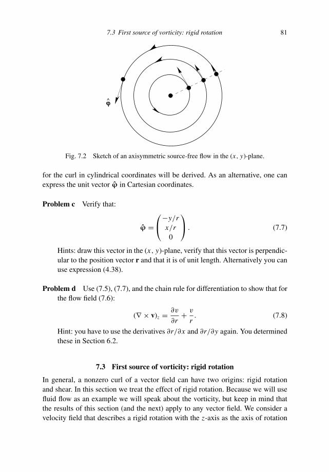
7.3 First source of vorticity: rigid rotation 81
j
Fig. 7.2 Sketch of an axisymmetric source-free flow in the (x, y)-plane.
for the curl in cylindrical coordinates will be derived. As an alternative, one canexpress the unit vector ϕ in Cartesian coordinates.
Problem c Verify that:
ϕ =⎛
⎝
−y/rx/r0
⎞
⎠ . (7.7)
Hints: draw this vector in the (x, y)-plane, verify that this vector is perpendic-ular to the position vector r and that it is of unit length. Alternatively you canuse expression (4.38).
Problem d Use (7.5), (7.7), and the chain rule for differentiation to show that forthe flow field (7.6):
(∇ × v)z = ∂v
∂r+ v
r. (7.8)
Hint: you have to use the derivatives ∂r/∂x and ∂r/∂y again. You determinedthese in Section 6.2.
7.3 First source of vorticity: rigid rotation
In general, a nonzero curl of a vector field can have two origins: rigid rotationand shear. In this section we treat the effect of rigid rotation. Because we will usefluid flow as an example we will speak about the vorticity, but keep in mind thatthe results of this section (and the next) apply to any vector field. We consider avelocity field that describes a rigid rotation with the z-axis as the axis of rotation
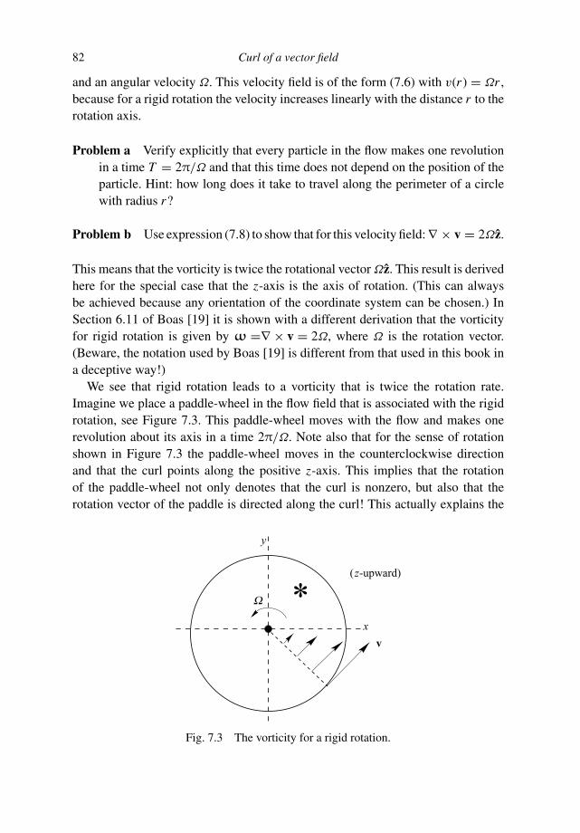
82 Curl of a vector field
and an angular velocity Ω. This velocity field is of the form (7.6) with v(r ) = Ωr ,because for a rigid rotation the velocity increases linearly with the distance r to therotation axis.
Problem a Verify explicitly that every particle in the flow makes one revolutionin a time T = 2π/Ω and that this time does not depend on the position of theparticle. Hint: how long does it take to travel along the perimeter of a circlewith radius r?
Problem b Use expression (7.8) to show that for this velocity field: ∇ × v = 2Ωz.
This means that the vorticity is twice the rotational vector Ωz. This result is derivedhere for the special case that the z-axis is the axis of rotation. (This can alwaysbe achieved because any orientation of the coordinate system can be chosen.) InSection 6.11 of Boas [19] it is shown with a different derivation that the vorticityfor rigid rotation is given by ω =∇ × v = 2Ω, where Ω is the rotation vector.(Beware, the notation used by Boas [19] is different from that used in this book ina deceptive way!)
We see that rigid rotation leads to a vorticity that is twice the rotation rate.Imagine we place a paddle-wheel in the flow field that is associated with the rigidrotation, see Figure 7.3. This paddle-wheel moves with the flow and makes onerevolution about its axis in a time 2π/Ω. Note also that for the sense of rotationshown in Figure 7.3 the paddle-wheel moves in the counterclockwise directionand that the curl points along the positive z-axis. This implies that the rotationof the paddle-wheel not only denotes that the curl is nonzero, but also that therotation vector of the paddle is directed along the curl! This actually explains the
z( -upward)
W
y
x
*v
Fig. 7.3 The vorticity for a rigid rotation.
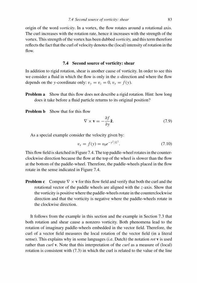
7.4 Second source of vorticity: shear 83
origin of the word vorticity. In a vortex, the flow rotates around a rotational axis.The curl increases with the rotation rate, hence it increases with the strength of thevortex. This strength of the vortex has been dubbed vorticity, and this term thereforereflects the fact that the curl of velocity denotes the (local) intensity of rotation in theflow.
7.4 Second source of vorticity: shear
In addition to rigid rotation, shear is another cause of vorticity. In order to see thiswe consider a fluid in which the flow is only in the x-direction and where the flowdepends on the y-coordinate only: vy = vz = 0, vx = f (y).
Problem a Show that this flow does not describe a rigid rotation. Hint: how longdoes it take before a fluid particle returns to its original position?
Problem b Show that for this flow
∇ × v = −∂ f
∂yz. (7.9)
As a special example consider the velocity given by:
vx = f (y) = v0e−y2/L2. (7.10)
This flow field is sketched in Figure 7.4. The top paddle-wheel rotates in the counter-clockwise direction because the flow at the top of the wheel is slower than the flowat the bottom of the paddle-wheel. Therefore, the paddle-wheels placed in the flowrotate in the sense indicated in Figure 7.4.
Problem c Compute ∇ × v for this flow field and verify that both the curl and therotational vector of the paddle wheels are aligned with the z-axis. Show thatthe vorticity is positive where the paddle-wheels rotate in the counterclockwisedirection and that the vorticity is negative where the paddle-wheels rotate inthe clockwise direction.
It follows from the example in this section and the example in Section 7.3 thatboth rotation and shear cause a nonzero vorticity. Both phenomena lead to therotation of imaginary paddle-wheels embedded in the vector field. Therefore, thecurl of a vector field measures the local rotation of the vector field (in a literalsense). This explains why in some languages (i.e. Dutch) the notation rot v is usedrather than curl v. Note that this interpretation of the curl as a measure of (local)rotation is consistent with (7.3) in which the curl is related to the value of the line

84 Curl of a vector field
z( -upward)
y
x*
*
Fig. 7.4 Sketch of the flow field for a shear flow.
integral along the small contour. If the flow (locally) rotates and if we integratealong the fluid flow, the line integral
∮
v · dr will be relatively large, so that thisline integral indeed measures the local rotation.
Rotation and shear each contribute to the curl of a vector field. Let us consideronce again a vector field of the form (7.6) which is axially symmetric around thez-axis. In the following we do not require the rotation around the z-axis to be rigid,so that v(r ) in (7.6) is arbitrary. We know that both the rotation around the z-axisand the shear are a source of vorticity.
Problem d Show that for the flow
v(r ) = A
r(7.11)
the vorticity vanishes, with A a constant that is not yet determined. Make asketch of this flow field.
The vorticity of this flow vanishes despite the fact that the flow rotates around thez-axis (but not in rigid rotation) and that the flow has a nonzero shear. The reasonthat the vorticity vanishes is that the contribution of the rotation around the z-axis tothe vorticity is equal but of opposite sign to the contribution of the shear, so that thetotal vorticity vanishes. Note that this implies that a paddle-wheel does not changeits orientation as it moves with this flow!

7.5 Magnetic field induced by a straight current 85
7.5 Magnetic field induced by a straight current
At this point you may have the impression that the flow field (7.11) has beencontrived in an artificial way. However, keep in mind that all the arguments of theprevious section apply to any vector field and that fluid flow was used only as anexample to fix our mind. As an example we consider the generation of the magneticfield B by an electrical current J that is independent of time. The Maxwell equationfor the curl of the magnetic field in vacuum is for time-independent fields givenby:
∇ × B = µ0J, (7.12)
see equation (5.22) in reference [53]. In this expression µ0 is the magnetic per-meability of vacuum. It plays the role of a coupling constant since it governs thestrength of the magnetic field that is generated by a given current. It plays the samerole as 1/permittivity in (6.23) or the gravitational constant G in (6.33). The vectorJ denotes the electric current per unit volume (properly called the electric currentdensity).
For simplicity we consider an electric current running through an infinite straightwire along the z-axis. Because of rotational symmetry around the z-axis and becauseof translational invariance along the z-axis the magnetic field depends neither on ϕ
nor on z and must be of the form (7.6). Away from the wire the electrical current Jvanishes.
Problem a Use the results of problem b of the previous section to show that
B = A
rϕ. (7.13)
A comparison with equation (7.11) shows that for this magnetic field the contri-bution of the “rotation” around the z-axis to ∇ × B is exactly balanced by thecontribution of the “magnetic shear” to ∇ × B. It should be noted that the magneticfield derived in this section is of great importance because this field has been usedto define the unit of electrical current, the ampere. However, this can only be donewhen the constant A in expression (7.13) is known.
Problem b Why does the treatment of this section not tell us what the relation isbetween the constant A and the current J in the wire?
We return to this issue in Section 9.3.
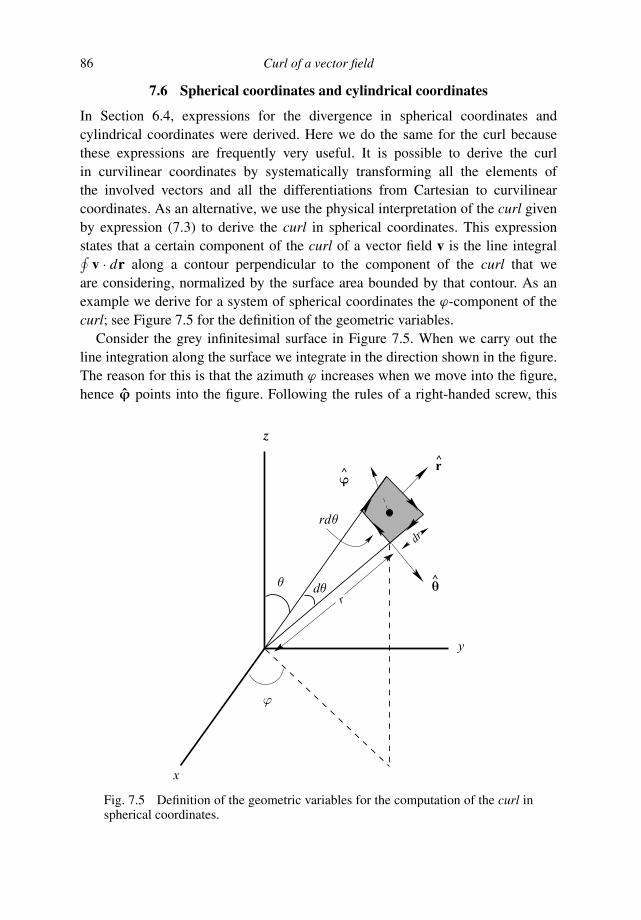
86 Curl of a vector field
7.6 Spherical coordinates and cylindrical coordinates
In Section 6.4, expressions for the divergence in spherical coordinates andcylindrical coordinates were derived. Here we do the same for the curl becausethese expressions are frequently very useful. It is possible to derive the curlin curvilinear coordinates by systematically transforming all the elements ofthe involved vectors and all the differentiations from Cartesian to curvilinearcoordinates. As an alternative, we use the physical interpretation of the curl givenby expression (7.3) to derive the curl in spherical coordinates. This expressionstates that a certain component of the curl of a vector field v is the line integral∮
v · dr along a contour perpendicular to the component of the curl that weare considering, normalized by the surface area bounded by that contour. As anexample we derive for a system of spherical coordinates the ϕ-component of thecurl; see Figure 7.5 for the definition of the geometric variables.
Consider the grey infinitesimal surface in Figure 7.5. When we carry out theline integration along the surface we integrate in the direction shown in the figure.The reason for this is that the azimuth ϕ increases when we move into the figure,hence ϕ points into the figure. Following the rules of a right-handed screw, this
^r^
rd
y
x
z
^
dr
r
Fig. 7.5 Definition of the geometric variables for the computation of the curl inspherical coordinates.

7.6 Spherical coordinates and cylindrical coordinates 87
corresponds to the indicated sense of integration. The area enclosed by the contouris given by rdθdr . By summing the contributions of the four sides of the contourwe find, using expression (7.3), that the ϕ-component of ∇ × v is given by:
(∇ × v)ϕ = 1
rdθdr[vθ (r + dr, θ )(r + dr ) dθ − vr (r, θ + dθ ) dr
− vθ (r, θ )rdθ + vr (r, θ ) dr ]. (7.14)
In this expression vr and vθ denote the components of v in the radial direction andin the direction of θ respectively.
Problem a Make sure that expression (7.14) is understood.
This result can be simplified by Taylor expanding the components of v in dr anddθ and linearizing the resulting expression in the infinitesimal increments dr anddθ .
Problem b Do this and show that the final result does not depend on dr and dθ
and is given by:
(∇ × v)ϕ = 1
r
∂
∂r(rvθ ) − 1
r
∂vr
∂θ. (7.15)
The same treatment can be applied to the other components of the curl. This leadsto the following expression for the curl in spherical coordinates:
∇ × v = r1
r sin θ
[
∂
∂θ
(
sin θ vϕ
) − ∂vθ
∂ϕ
]
+ θ1
r
[
1
sin θ
∂vr
∂ϕ− ∂
∂r
(
rvϕ
)
]
+ ϕ1
r
[
∂
∂r(rvθ ) − ∂vr
∂θ
]
. (7.16)
Problem c Use a similar analysis to show that in cylindrical coordinates (r, ϕ, z)the curl is given by:
∇ × v = r[
1
r
∂vz
∂ϕ− ∂vϕ
∂z
]
+ ϕ
[
∂vr
∂z− ∂vz
∂r
]
+ z1
r
[
∂
∂r
(
rvϕ
) − ∂vr
∂ϕ
]
,
(7.17)
with r =√
x2 + y2.
Problem d Use this result to re-derive (7.8) for vector fields of the form v =v(r )ϕ. Hint: use the same method as used in the derivation of (7.14) and treatthe three components of the curl separately.
8
Theorem of Gauss
In Section 6.5 we determined the gravitational field in N dimensions using as theonly ingredient that in free space, where the mass-density vanishes, the divergenceof the gravitational field vanishes: (∇ · g) = 0. This was sufficient to determine thegravitational field in expression (6.37). However, that expression is not quite satis-factory because it contains a constant A that is unknown. In fact, at this point wehave no idea how this constant is related to the mass M that causes the gravitationalfield! The reason for this is simple: in order to derive the gravitational field in (6.37)we have only used the field equation (6.33) for free space (where ρ = 0). However,if we want to find the relation between the mass and the resulting gravitational fieldwe must also use the field equation (∇ · g) = −4πGρ at places where the mass ispresent. More specifically, we have to integrate the field equation in order to findthe total effect of the mass. The theorem of Gauss gives us an expression for thevolume integral of the divergence of a vector field.
8.1 Statement of Gauss’s law
In Section 6.2 it was shown that the divergence is the flux per unit volume. In fact,expression (6.8) gives us the outward flux dΦv through an infinitesimal volume dV :dΦv = (∇ · v)dV . We can integrate this expression to find the total flux throughthe surface S which encloses the total volume V :
∮
Sv · dS =
∫
V(∇ · v) dV . (8.1)
In deriving this, equation (6.8) has been used to express the total flux on the left-handside. This expression is called the theorem of Gauss.
Note that in the derivation of (8.1) we did not use the dimensionality of thespace; this relation holds in any number of dimensions. You may recognize the
88
8.2 Gravitational field of a spherically symmetric mass 89
one-dimensional version of (8.1). In one dimension the vector v has only onecomponent vx , hence (∇ · v) = ∂xvx . A “volume” in one dimension is simply aline. Let this line run from x = a to x = b. The “surface” of a one-dimensionalvolume consists of the endpoints of this line, so that the left-hand side of (8.1) isthe difference of the function vx at its endpoints. This implies that the theorem ofGauss in one-dimension is:
vx (b) − vx (a) =∫ b
a
∂vx
∂xdx . (8.2)
This expression will be familiar to you. We will use the two-dimensional versionof the theorem of Gauss in Section 9.2 to derive the theorem of Stokes.
Problem a Compute the flux of the vector field v(x, y, z) = (x + y + z)z througha sphere of radius R centered on the origin by explicitly computing the integralthat defines the flux.
Problem b Solve problem a using Gauss’s law (8.1).
8.2 Gravitational field of a spherically symmetric mass
In this section we use Gauss’s law (8.1) to show that the gravitational field of abody with a spherically symmetric mass-density ρ depends only on the total massand not on the distribution of the mass over that body. For a spherically symmetricbody the mass-density depends only on radius: ρ = ρ(r ). Because of the sphericalsymmetry of the mass, the gravitational field is spherically symmetric and pointsin the radial direction:
g(r) = g(r )r. (8.3)
Problem a Use the field equation (6.33) for the gravitational field and Gauss’slaw applied to a surface that completely encloses the mass to show that
∮
Sg · dS = −4πG M, (8.4)
where M = ∫
V ρdV is the total mass of the body.
Problem b Use a sphere of radius r as the surface in (8.4) to show that thegravitational field is given in three dimensions by
g(r) = −G M
r2r. (8.5)
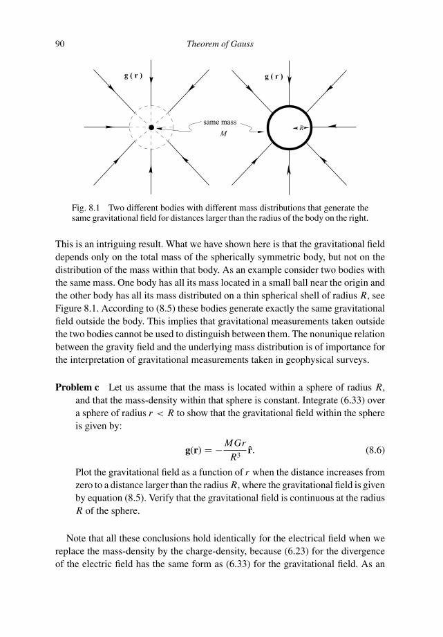
90 Theorem of Gauss
RM
same mass
g ( r ) g ( r )
Fig. 8.1 Two different bodies with different mass distributions that generate thesame gravitational field for distances larger than the radius of the body on the right.
This is an intriguing result. What we have shown here is that the gravitational fielddepends only on the total mass of the spherically symmetric body, but not on thedistribution of the mass within that body. As an example consider two bodies withthe same mass. One body has all its mass located in a small ball near the origin andthe other body has all its mass distributed on a thin spherical shell of radius R, seeFigure 8.1. According to (8.5) these bodies generate exactly the same gravitationalfield outside the body. This implies that gravitational measurements taken outsidethe two bodies cannot be used to distinguish between them. The nonunique relationbetween the gravity field and the underlying mass distribution is of importance forthe interpretation of gravitational measurements taken in geophysical surveys.
Problem c Let us assume that the mass is located within a sphere of radius R,and that the mass-density within that sphere is constant. Integrate (6.33) overa sphere of radius r < R to show that the gravitational field within the sphereis given by:
g(r) = − MGr
R3r. (8.6)
Plot the gravitational field as a function of r when the distance increases fromzero to a distance larger than the radius R, where the gravitational field is givenby equation (8.5). Verify that the gravitational field is continuous at the radiusR of the sphere.
Note that all these conclusions hold identically for the electrical field when wereplace the mass-density by the charge-density, because (6.23) for the divergenceof the electric field has the same form as (6.33) for the gravitational field. As an
8.3 Representation theorem for acoustic waves 91
example we consider a hollow spherical shell of radius R. On the spherical shellelectrical charge is distributed with a constant charge density: ρ = const .
Problem d Use expression (6.23) for the electric field and Gauss’s law to showthat within the hollow sphere the electric field vanishes: E(r) = 0 for r < R.
This result implies that when a charge is placed within such a spherical shell theelectrical field generated by the charge distribution on the shell exerts no net forceon this charge; the charge will not move. Since the electrical potential satisfiesE = −∇V , the result derived in problem d implies that the potential is constantwithin the sphere. This property has actually been used to determine experimentallywhether the electric field indeed satisfies (6.23) (which implies that the field of pointcharge decays as 1/r2). Measurements of the potential differences within a hollowspherical shell as described in problem d can be carried out with great sensitivity.Experiments based on this principle (usually in a more elaborate form) have beenused to ascertain the decay of the electric field of a point charge with distance.Writing the field strength as 1/r2+ε it has been shown that ε = (2.7 ± 3.1) × 10−16,see Section I.2 of Jackson [53] for a discussion. The small value of ε is a remarkableexperimental confirmation of (6.23) for the electric field.
8.3 Representation theorem for acoustic waves
Acoustic waves are waves that propagate through a gas or fluid. You can hear thevoice of others because acoustic waves propagate from their vocal tract to your ear.Acoustic waves are frequently used to describe the propagation of waves throughthe Earth. Since the Earth is a solid body, this is strictly speaking not correct,but under certain conditions (small scattering angles) the errors can be acceptable.The pressure field p(r) of acoustic waves satisfies the following partial differentialequation in the frequency domain:
∇ ·(
1
ρ∇ p
)
+ ω2
κp = f. (8.7)
In this expression ρ(r) is the mass-density of the medium, ω is the angular frequencyand κ(r) is the compressibility (a factor that describes how strongly the mediumresists changes in its volume). The right-hand side f (r) describes the source of theacoustic wave. This term accounts, for example, for the action of your voice.
We now consider two pressure fields p1(r) and p2(r) that both satisfy (8.7) withsources f1(r) and f2(r) on the right-hand side of the equation.
92 Theorem of Gauss
Problem a Multiply equation (8.7) for p1 with p2, multiply equation (8.7) forp2 with p1 and subtract the resulting expressions. Integrate the result over avolume V to show that:
∫
V
[
p2∇ ·(
1
ρ∇ p1
)
− p1∇ ·(
1
ρ∇ p2
)]
dV =∫
V(p2 f1 − p1 f2) dV . (8.8)
Ultimately we want to relate the wave field at the surface S that encloses the volumeV to the wave field within the volume. Obviously, Gauss’s law is the tool for doingthis. The problem we face is that Gauss’s law holds for the volume integral ofthe divergence, whereas in (8.8) we have the product of a divergence (such as∇ · (
ρ−1∇ p1)
) with another function (such as p2). This means we have to “make”a divergence.
Problem b First derive that
∇ · ( f v) = f (∇ · v) + v · ∇ f. (8.9)
Hint: write the left-hand side in its components and use the product rule fordifferentiation.
Problem c Use f = p2 and v = ρ−1∇ p1 in (8.9) to show that
p2∇ ·(
1
ρ∇ p1
)
= ∇ ·(
1
ρp2∇ p1
)
− 1
ρ(∇ p1 · ∇ p2). (8.10)
What we are doing here is similar to the standard derivation of integra-tion by parts. The easiest way to show that
∫ ba f (∂g/∂x)dx = [ f (x)g(x)]b
a −∫ b
a (∂ f/∂x)gdx is to integrate the identity f (∂g/∂x) = ∂( f g)/dx − (∂ f/∂x)g fromx = a to x = b. This last equation has exactly the same structure as (8.10).
Problem d Use (8.8), (8.10), and Gauss’s law to derive that∮
S
1
ρ(p2∇ p1 − p1∇ p2) · dS =
∫
V(p2 f1 − p1 f2) dV . (8.11)
To see the power of this expression, consider the special case that the source f2 ofp2 is of unit strength and that this source is localized in a very small volume arounda point r0 within the volume. This means that f2 on the right-hand side of (8.11) isonly nonzero at r0. The corresponding volume integral
∫
V p1 f2dV is in that casegiven by p1(r0). The wavefield p2(r) generated by this point source is called theGreen’s function, and this special solution is denoted by G(r, r0). (The concept ofthe Green’s function is introduced in great detail in Chapter 18.) The argument r0
is added to indicate that this is the wavefield at location r due to a unit source at

8.4 Flowing probability 93
location r0. We now consider a solution p1 that has no sources within the volumeV (i.e. f1 = 0). Let us simplify the notation further by dropping the subscript “1”in p1.
Problem e Show by making all these changes that (8.11) can be written as:
p(r0) =∮
S
1
ρ[p(r)∇G(r, r0) − G(r, r0)∇ p(r)] · dS. (8.12)
This result is called the “representation theorem” because it gives the wave-field inside the volume when the wavefield (and its gradient) are specified on thesurface that bounds this volume. Expression (8.12) can be used to formally de-rive Huygens’s principle which states that every point on a wavefront acts as asource for other waves and that interference between these waves determines thepropagation of the wavefront. Equation (8.12) also forms the basis for imagingtechniques for seismic data [93]. In seismic exploration one records the wavefieldat the Earth’s surface. This can be used by taking the Earth’s surface as the sur-face S over which the integration is carried out. If the Green’s function G(r, r0)is known, one can use expression (8.12) to compute the wavefield in the interiorof the Earth. Once the wavefield in the interior of the Earth is known, one candeduce some of the properties of the material in the Earth. In this way, equation(8.12) (or its generalization to elastic waves [3]) forms the basis of seismic imagingtechniques.
This treatment suggests that if one knows the wavefield at a surface, one candetermine the wavefield anywhere within the surface, and hence one can determinethe properties of the medium within the surface. This in turn suggests that theproblem of seismic imaging has been solved by the treatment of this section. Thereis, however, a catch. In order to apply (8.12) one must know the Green’s functionG. To know this function one must know the medium. We thus have the interestingsituation that once we know the Green’s function, we can deduce the properties ofthe medium from (8.12), but that in order to use the Green’s function we must knowthe medium. This suggests that seismic imaging cannot be carried out. Fortunately,it turns out that in practice it suffices to use a reasonable estimate of the Green’sfunction in (8.12). Such an estimated Green’s function can be computed once thevelocity in the medium is reasonably well known. It is for this reason that velocityestimation is such a crucial step in seismic data processing [28, 123].
8.4 Flowing probability
In classical mechanics, the motion of a particle with mass m is governed by Newton’slaw: mr = F. When the force F is associated with a potential V (r) the motion of
94 Theorem of Gauss
the particle satisfies:
md2rdt2
= −∇V (r). (8.13)
Newton’s law, however, does not hold for particles that are very small. Atomicparticles such as electrons are not described accurately by (8.13). One of the out-standing features of quantum mechanics is that an atomic particle is treated as awave that describes the properties of that particle. This rather vague statement re-flects the wave-particle duality that forms the basis of quantum mechanics. Thewavefunction ψ(r,t) that describes a particle that moves under the influence of apotential V (r) satisfies the Schrodinger equation:
‡
ih∂ψ(r, t)
∂t= − h2
2m∇2ψ(r, t) + V (r)ψ(r, t). (8.14)
In this expression, h is Planck’s constant h divided by 2π; where Planck’s constanthas the numerical value h = 6.626 × 10⁻³⁴ kg m2/s.
Suppose we are willing to accept that the motion of an electron is described bythe Schrodinger equation, then the following question arises: What is the positionof the electron as a function of time? According to the Copenhagen interpretationof quantum mechanics, this is a meaningless question because the electron behaveslike a wave and does not have a definite location. Instead, the wavefunction ψ(r, t)dictates how likely it is that the particle is at location r at time t . Specifically, thequantity |ψ(r, t)|2 is the probability-density of finding the particle at location rat time t . This implies that the probability PV that the particle is located withinthe volume V is given by PV = ∫
V |ψ |2dV . (Take care not to confuse the volumewith the potential, because they are both indicated with the same symbol V .) Thisimplies that the wavefunction is related to a probability. Instead of the motion of theelectron, Schrodinger’s equation dictates how the probability-density of the particlemoves through space as time progresses. One expects that a “probability current”is associated with this movement. In this section we determine this current usingthe theorem of Gauss.
Problem a In the following we need the time derivative of ψ∗(r, t), where theasterisk denotes the complex conjugate. Derive the differential equation thatψ∗(r, t) obeys by taking the complex conjugate of Schrodinger’s equation(8.14).
‡In this expression ∇2 stands for the Laplacian which is treated in Chapter 10. At this point you only need to knowthat the Laplacian of a function is the divergence of the gradient of that function: ∇2ψ = div grad ψ = ∇ · ∇ψ .
8.4 Flowing probability 95
Problem b Use this result to derive that for a volume V that is fixed in time:
∂
∂t
∫
V|ψ |2dV = ih
2m
∫
V(ψ∗∇2ψ − ψ∇2ψ∗)dV . (8.15)
Hint: use that∂
∂t|ψ |2 = ∂
∂t(ψψ∗) = ψ
∂ψ∗
∂t+ ψ∗ ∂ψ
∂t, and use (8.14) and
the result of problem a.
Problem c Use Gauss’s law to rewrite this expression as:
∂
∂t
∫
V|ψ |2dV = ih
2m
∮
(ψ∗∇ψ − ψ∇ψ∗) · dS. (8.16)
Hint: use a treatment similar to expression (8.10).
The left-hand side of this expression gives the time derivative of the probability thatthe particle is within the volume V . The only way the particle can enter or leave thevolume is through the enclosing surface S. The right-hand side therefore describesthe “flow” of probability through the surface S. More accurately, one can formulatethis as the flux of the probability-density current. This means that expression (8.16)can be written as
∂ PV
∂t= −
∫
J · dS, (8.17)
where the probability-density current J is given by:
J = ih
2m(ψ∇ψ∗ − ψ∗∇ψ). (8.18)
As an example let us consider a plane wave:
ψ(r, t) = A ei(k·r−ωt), (8.19)
where k is the wavevector and A an unspecified constant.
Problem d Show that the wavelength λ is related to the wavevector by the relationλ = 2π/ |k|. In which direction does the wave propagate?
Problem e Show that the probability-density current J for this wavefunction sat-isfies:
J = hkm
|ψ |2. (8.20)
This is a very interesting expression. The term |ψ |2 gives the probability-density ofthe particle, while the probability-density current J physically describes the current
96 Theorem of Gauss
of this probability-density. Since the probability-density current moves with thevelocity of the particle, the remaining terms on the right-hand side of (8.20) mustdenote the velocity of the particle:
v = hkm
. (8.21)
Since the momentum p is the mass times the velocity, (8.21) can also be writtenas p = hk. This relation was proposed by de Broglie in 1924 using completelydifferent arguments than those we have used here [22]. Its discovery was a majorstep in the development of quantum mechanics.
Problem f Use this expression and the result of problem e to compute your ownwavelength while you are riding your bicycle. Are quantum-mechanical phe-nomena important when you ride your bicycle? Use your wavelength as anargument. Did you know you possessed a wavelength?

9
Theorem of Stokes
In Chapter 8 we noted that in order to find the gravitational field of a mass we haveto integrate the field equation (6.33) over the mass. Gauss’s theorem can then beused to compute the integral of the divergence of the gravitational field. For the curlthe situation is similar. In Section 7.5 we computed the magnetic field generatedby a current in a straight infinite wire. The field equation
∇ × B = µ0J (7.12)
was used to compute the field away from the wire. However, the solution (7.13)contained an unknown constant A. The reason for this is that the field equation(7.12) was only used outside the wire, where J = 0. The treatment of Section 7.5therefore did not provide us with the relation between the field B and its source J.The only way to obtain this relation is to integrate the field equation. This implieswe have to compute the integral of the curl of a vector field. The theorem of Stokestells us how to do this.
9.1 Statement of Stokes’s law
The theorem of Stokes is based on the principle that the curl of a vector field isthe closed line integral of the vector field per unit surface area, see Section 7.1.Mathematically this statement is expressed by (7.2) which we write in a slightlydifferent form as:
∮
dSv · dr = (∇ × v) · n d S = (∇ × v) · dS. (9.1)
The only difference with (7.2) is that in the above expression we have not aligned thez-axis with the vector ∇ × v. The infinitesimal surface is therefore not necessarilyconfined to the (x, y)-plane and the z-component of the curl is replaced by thecomponent of the curl normal to the surface, hence the occurrence of the terms
97

98 Theorem of Stokes
n
n
or
Fig. 9.1 The relation between the sense of integration and the orientation of thesurface.
nd S in (9.1). Expression (9.1) holds for an infinitesimal surface area. However, thisexpression can immediately be integrated to give the surface integral of the curlover a finite surface S that is bounded by the curve C :
∮
Cv · dr =
∫
S(∇ × v) · dS. (9.2)
This result is known as the theorem of Stokes (or Stokes’s law). The line integral onthe left-hand side is over the curve that bounds the surface S. A proper derivationof Stokes’s law can be found in reference [68].
Note that a line integration along a closed surface can be carried out in twodirections. What is the direction of the line integral on the left-hand side of Stokes’slaw (9.2)? To see this, we have to realize that Stokes’s law was ultimately based on(7.2). The orientation of the line integration used in that expression is defined inFigure 7.1 , where it can be seen that the line integration is in the counterclockwisedirection. In Figure 7.1 the z-axis points out of the paper, which implies that thevector dS also points out of the paper. This means that in Stokes’s law the sense ofthe line integration and the direction of the surface vector dS are related throughthe rule for a right-handed screw. This orientation is indicated in Figure 9.1.
There is something strange about Stokes’s law. If we define a curve C over whichwe carry out the line integration, we can define many different surfaces S that arebounded by the same curve C . Apparently, the surface integral on the right-handside of Stokes’s law does not depend on the specific choice of the surface S as longas it is bounded by the curve C .
Problem a Let us verify this property for an example. Consider the vector fieldv = rϕ. Let the curve C used for the line integral be a circle in the (x, y)-plane of radius R, see Figure 9.2 for the geometry of the problem. (i) Computethe line integral on the left-hand side of (9.2) by direct integration. Computethe surface integral on the right-hand side of (9.2) by (ii) integrating over

9.1 Statement of Stokes’s law 99
S2
S1
z
x
y
C
Fig. 9.2 Definition of the geometric variables for problem a.
S1
S2
C
Fig. 9.3 Two surfaces that are bounded by the same contour C .
a disc of radius R in the (x, y)-plane (the surface S1 in Figure 9.2) and by(iii) integrating over the upper half of a sphere with radius R (the surface S2
in Figure 9.2). Verify that the three integrals are identical.
It is actually not difficult to prove that the surface integral in Stokes’s law is inde-pendent of the specific choice of the surface S as long as it is bounded by the samecontour C . Consider Figure 9.3 where the two surfaces S1 and S2 are bounded bythe same contour C . We want to show that the surface integral of ∇ × v is the samefor the two surfaces, that is that:
∫
S1
(∇ × v) · dS =∫
S2
(∇ × v) · dS. (9.3)
We can form a closed surface S by combining the surfaces S1 and S2.

100 Theorem of Stokes
Problem b Show that (9.3) is equivalent to the condition∮
S(∇ × v) · dS = 0, (9.4)
where the integration is over the closed surfaces defined by the combinationof S1 and S2. Pay particular attention to the signs of the different terms.
Problem c Use Gauss’s law to convert (9.4) to a volume integral and show thatthe integral is indeed identical to zero. In doing so you need to use the identity∇ · (∇ × v) = 0 (or in another notation div curl v = 0). Make sure you canderive this identity.
The result you obtained in problem c implies that condition (9.3) is indeed satisfiedand that in the application of Stokes’s law you can choose any surface as long asit is bounded by the contour over which the line integration is carried out. Thisis a very useful result because often the surface integration can be simplified bychoosing the surface carefully.
9.2 Stokes’s theorem from the theorem of Gauss
Stokes’s law is concerned with surface integrations. Since the curl is intrinsically athree-dimensional vector, Stokes’s law is inherently related to three space dimen-sions. However, if we consider a vector field that depends only on the coordinates xand y (v = v(x, y)) and that has a vanishing component in the z-direction (vz = 0),then ∇ × v points along the z-axis. If we consider a contour C that is confined tothe (x, y)-plane, for such a vector field Stokes’s law (9.2) takes the form
∮
C(vx dx + vydy) =
∫
S
(
∂xvy − ∂yvx)
dxdy. (9.5)
Problem a Verify this.
This result can be derived from the theorem of Gauss in two dimensions.
Problem b Show that Gauss’s law (8.1) for a vector field u in two dimensionscan be written as
∮
C(u · n)ds =
∫
S(∂x ux + ∂yuy)dxdy, (9.6)
where the unit vector n is perpendicular to the curve C (see Figure 9.4) andwhere ds denotes the integration over the arclength of the curve C .

9.2 Stokes’s theorem from the theorem of Gauss 101
nt^
v
u
Fig. 9.4 Definition of the geometric variables for the derivation of Stokes’s lawfrom the theorem of Gauss.
In order to derive the special form of Stokes’s law (9.5) from Gauss’s law (9.6) wehave to define the relation between the vectors u and v. Let the vector u followfrom v by a clockwise rotation over 90 degrees, see Figure 9.4.
Problem c Show that:
vx = −uy and vy = ux . (9.7)
We now define the unit vector t to be directed along the curve C , see Figure 9.4.Since a rotation is an orthonormal transformation, the inner product of two vectorsis invariant for a rotation over 90 degrees so that (u · n) = (v · t).
Problem d Verify this by expressing the components of t in the components ofn and by using (9.7). The change in the position vector along the curve C isgiven by
dr = t ds =(
dxdy
)
. (9.8)
Problem e Use these results to show that (9.5) follows from (9.6).
What you have shown here is that Stokes’s law for the special case considered inthis section is identical to the theorem of Gauss for two spatial dimensions.
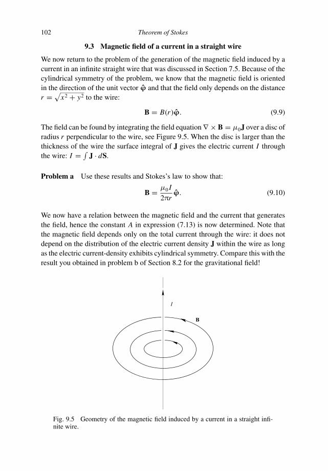
102 Theorem of Stokes
9.3 Magnetic field of a current in a straight wire
We now return to the problem of the generation of the magnetic field induced by acurrent in an infinite straight wire that was discussed in Section 7.5. Because of thecylindrical symmetry of the problem, we know that the magnetic field is orientedin the direction of the unit vector ϕ and that the field only depends on the distancer =
√
x2 + y2 to the wire:
B = B(r )ϕ. (9.9)
The field can be found by integrating the field equation ∇ × B = µ0J over a disc ofradius r perpendicular to the wire, see Figure 9.5. When the disc is larger than thethickness of the wire the surface integral of J gives the electric current I throughthe wire: I = ∫
J · dS.
Problem a Use these results and Stokes’s law to show that:
B = µ0 I
2πrϕ. (9.10)
We now have a relation between the magnetic field and the current that generatesthe field, hence the constant A in expression (7.13) is now determined. Note thatthe magnetic field depends only on the total current through the wire: it does notdepend on the distribution of the electric current density J within the wire as longas the electric current-density exhibits cylindrical symmetry. Compare this with theresult you obtained in problem b of Section 8.2 for the gravitational field!
I
B
Fig. 9.5 Geometry of the magnetic field induced by a current in a straight infi-nite wire.
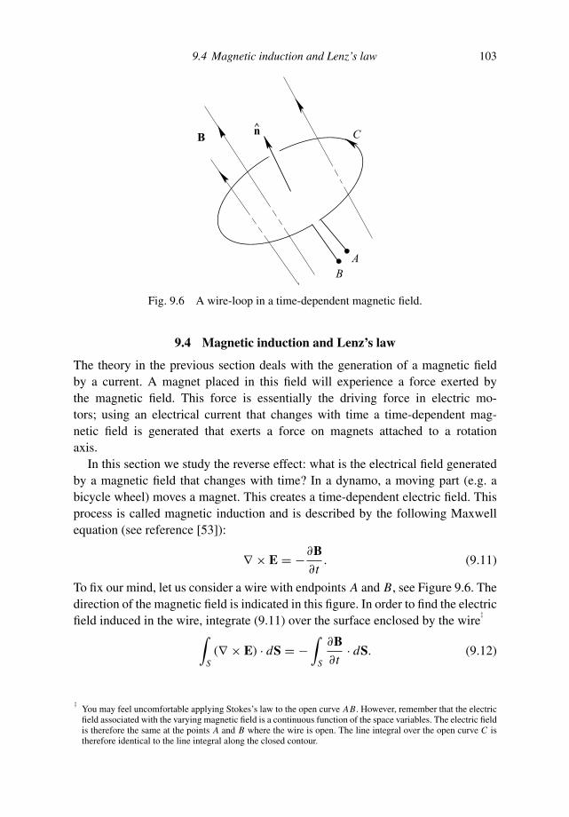
9.4 Magnetic induction and Lenz’s law 103
Bn
B
^
A
C
Fig. 9.6 A wire-loop in a time-dependent magnetic field.
9.4 Magnetic induction and Lenz’s law
The theory in the previous section deals with the generation of a magnetic fieldby a current. A magnet placed in this field will experience a force exerted bythe magnetic field. This force is essentially the driving force in electric mo-tors; using an electrical current that changes with time a time-dependent mag-netic field is generated that exerts a force on magnets attached to a rotationaxis.
In this section we study the reverse effect: what is the electrical field generatedby a magnetic field that changes with time? In a dynamo, a moving part (e.g. abicycle wheel) moves a magnet. This creates a time-dependent electric field. Thisprocess is called magnetic induction and is described by the following Maxwellequation (see reference [53]):
∇ × E = −∂B∂t
. (9.11)
To fix our mind, let us consider a wire with endpoints A and B, see Figure 9.6. Thedirection of the magnetic field is indicated in this figure. In order to find the electricfield induced in the wire, integrate (9.11) over the surface enclosed by the wire
‡
∫
S(∇ × E) · dS = −
∫
S
∂B∂t
· dS. (9.12)
‡You may feel uncomfortable applying Stokes’s law to the open curve AB. However, remember that the electricfield associated with the varying magnetic field is a continuous function of the space variables. The electric fieldis therefore the same at the points A and B where the wire is open. The line integral over the open curve C istherefore identical to the line integral along the closed contour.
104 Theorem of Stokes
Problem a Show that the right-hand side of (9.12) is given by −∂Φ/∂t , where Φ
is the magnetic flux through the wire. (See Section 6.1 for the definition of theflux.)
We have discovered that a change in the magnetic flux is the source of an electricfield. The resulting field can be characterized by the electromotive force FAB, whichis a measure of the work done by the electric field on a unit charge when it movesfrom point A to point B, see Figure 9.6:
FAB ≡∫ B
AE · dr. (9.13)
Problem b Apply Stokes’s law to the left-hand side of expression (9.12) to showthat the electromotive force satisfies
FAB = − ∂ΦB
∂t. (9.14)
Problem c Because of the electromotive force an electric current will flow throughthe wire. Determine the direction of the electric current in the wire. Show thatthis current generates a magnetic field that opposes the change in the magneticfield that generates the current. You learned in Section 9.3 the direction of themagnetic field that is generated by an electric current in a wire.
What we have discovered in problem c is Lenz’s law, which states that inductioncurrents lead to a secondary magnetic field which opposes the change in the primarymagnetic field that generates the electric current. This implies that coils in electricalsystems exhibit a certain inertia in the sense that they resist changes in the magneticfield that passes through the coil. The amount of inertia is described by a quantitycalled the inductance L . This quantity plays a role similar to mass in classicalmechanics because the mass of a body also describes how strongly a body resistschanging its velocity when an external force is applied.
9.5 Aharonov–Bohm effect
It was shown in Section 6.3 that because of the absence of magnetic monopoles themagnetic field is source-free: (∇ · B) = 0. In electromagnetism one often expressesthe magnetic field as the curl of a vector field A:
B = ∇ × A. (9.15)

9.5 Aharonov–Bohm effect 105
The advantage of writing the magnetic field in this way is that for any field A themagnetic field satisfies (∇ · B) = 0 because ∇ · (∇ × A) = 0.
Problem a Give a proof of this last identity.
The vector field A is called the vector potential. The reason for this name is that itplays a role similar to the electric potential V . The electric and the magnetic fieldsfollow from V and A respectively by differentiation: E = −∇V and B = ∇ × A.The electric field vanishes when the potential V is constant. Since this constantmay be nonzero, this implies that the electric field may vanish but that the potentialis nonzero. The vector potential has a similar property, that is it can be nonzero(and variable) in parts of space where the magnetic field vanishes. As an example,consider a magnetic field with cylindrical symmetry along the z-axis which isconstant for r < R and which vanishes for r > R:
B =
B0z for r < R0 for r > R
; (9.16)
see Figure 9.7 for a sketch of the magnetic field. Because of the cylindrical symmetrythe vector potential is a function of the distance r to the z-axis only and does notdepend on z or ϕ.
Problem b Use expression (7.17) to show that a vector potential of the form
A = f (r )ϕ (9.17)
x
y
z
R
Fig. 9.7 Geometry of the magnetic field.
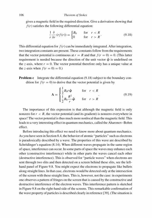
106 Theorem of Stokes
gives a magnetic field in the required direction. Give a derivation showing thatf (r ) satisfies the following differential equation:
1
r
∂
∂r(r f (r )) =
B0 for r < R0 for r > R
. (9.18)
This differential equation for f (r ) can be immediately integrated. After integration,two integration constants are present. These constants follow from the requirementsthat the vector potential is continuous at r = R and that f (r = 0) = 0. (This latterrequirement is needed because the direction of the unit vector ϕ is undefined onthe z-axis, where r = 0. The vector potential therefore only has a unique value atthe z-axis when f (r = 0) = 0.)
Problem c Integrate the differential equation (9.18) subject to the boundary con-dition for f (r = 0) to derive that the vector potential is given by
A =
⎧
⎪
⎨
⎪
⎩
1
2B0rϕ for r < R
1
2B0
R2
rϕ for r > R
. (9.19)
The importance of this expression is that although the magnetic field is onlynonzero for r < R, the vector potential (and its gradient) is nonzero everywhere inspace! The vector potential is thus much more nonlocal than the magnetic field. Thisleads to a very interesting effect in quantum mechanics, called the Aharonov–Bohmeffect.
Before introducing this effect we need to know more about quantum mechanics.As you have seen in Section 8.4, the behavior of atomic “particles” such as electronsis paradoxically described by a wave. The properties of this wave are described bySchrodinger’s equation (8.14). When different waves propagate in the same regionof space, interference can occur. In some parts of space the waves may enhance eachother (constructive interference) while in other parts the waves cancel each other(destructive interference). This is observed for “particle waves” when electrons aresent through two slits and then detected on a screen behind these slits, see the left-hand panel of Figure 9.8. You might expect the electrons to propagate like bulletsalong straight lines. In that case, electrons would be detected only at the intersectionof the screen with these straight lines. This is, however, not the case: in experimentsone observes a pattern of fringes on the screen that is caused by the constructive anddestructive interference of the electron waves. This interference pattern is sketchedin Figure 9.8 on the right-hand side of the screens. This remarkable confirmation ofthe wave property of particles is described clearly in reference [39]. (The situation is

9.5 Aharonov–Bohm effect 107
1
B
1
22
P
P
P
P
Fig. 9.8 Experiment in which electrons travel through two slits and are detectedon a screen behind the slits. The resulting interference pattern is sketched. Theexperiment without a magnetic field is shown on the left, the experiment with amagnetic field is shown on the right. Note the shift in the maxima and minima ofthe interference pattern between the two experiments.
even more remarkable when one sends the electrons through the slits “one-by-one”so that only one electron passes through the slits at a time. In that case one seesa dot at the detector for each electron. However, after many particles have arrivedat the detector this pattern of dots forms the interference pattern of the waves, seereference [94].)
Let us consider the same experiment, but with a magnetic field given by (9.16)placed between the two slits. When the electrons propagate along the paths P1 orP2 they do not pass through this field, hence one would expect that the electronswould not be influenced by this field and that the magnetic field would not changethe observed interference pattern at the detector. However, it is an observationalfact that the magnetic field does change the interference pattern at the detector, seereference [94] for examples. This surprising effect is called the Aharonov–Bohmeffect [2].
In order to understand this effect, we should note that a magnetic field in quantummechanics leads to a phase shift of the wavefunction. If the wavefunction in theabsence of a magnetic field is given by ψ(r), the wavefunction in the presence ofthe magnetic field is given by ψ(r)× exp[(ie/hc)
∫
P A · dr], see reference [91]. Inthis expression h is Planck’s constant (divided by 2π), c is the speed of light, and Ais the vector potential associated with the magnetic field. The integration is over thepath P from the source of the particles to the detector. Consider now the waves thatinterfere in the two-slit experiment in the right-hand panel of Figure 9.8. The wavethat travels through the upper slit experiences a phase shift exp[(ie/hc)
∫
P1A · dr],
where the integration is over the path P1 through the upper slit. The wave that

108 Theorem of Stokes
travels through the lower slit obtains a phase shift exp[(ie/hc)∫
P2A · dr] where the
path P2 runs through the lower slit.
Problem d Show that the phase difference δϕ between the two waves due to thepresence of the magnetic field is given by
δϕ = e
hc
∮
PA · dr, (9.20)
where the path P is the closed path from the source through the upper slit tothe detector and back through the lower slit to the source.
This phase difference affects the interference pattern because it is the relative phasebetween interfering waves that determines whether the interference is constructiveor destructive.
Problem e Use Stokes’s law and expression (9.15) to show that the phase differ-ence can be written as
δϕ = eΦB
hc, (9.21)
where ΦB is the magnetic flux through the area enclosed by the path P .
This expression shows that the phase shift between the interfering waves isproportional to the magnetic field enclosed by the paths of the interfering waves,despite the fact that the electrons never move through the magnetic field B. Mathe-matically the reason for this surprising effect is that the vector potential is nonzerothroughout space even when the magnetic field is confined to a small region ofspace, see (9.19) as an example. However, this explanation is purely mathematicaland does not seem to agree with common sense. This has led to speculations thatthe vector potential is actually a more “fundamental” quantity than the magneticfield [94].
9.6 Wingtips vortices
If you have watched aircraft closely, you may have noticed that sometimes a streamof condensation is left behind by the wingtips, see Figure 9.9. This is a differentcondensation trail than the thick contrails created by the engines. The condensationtrails that start at the wingtips are due to a vortex (a spinning motion of the air) thatis generated at the wingtips. This vortex is called the wingtip vortex. In this sectionwe use Stokes’s law to see that this wingtip vortex is closely related to the lift thatis generated by the airflow along a wing.

9.6 Wingtips vortices 109
Fig. 9.9 Vortices trailing from the wingtips of a Boeing 727. Figure courtesy ofNASA.
C
Fig. 9.10 Sketch of the flow along an airfoil. The wing is shown in grey, thecontour C is shown by the thick solid line.
Let us first consider the flow along a wing, see Figure 9.10. In the figure the airtraverses a longer path along the upper part of the wing than along the lower part.Because of the curved upper side of the wing, the velocity of the airstream alongthe upper part of the wing is larger than the velocity along the lower part.
Problem a The circulation is defined as the line integral∮
C v · dr of the veloc-ity along a curve. Is the circulation positive or negative for the curve C inFigure 9.10 for the indicated sense of integration? Use that the air movesfaster over the upper side of the wing than under the lower side.
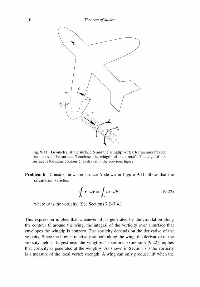
110 Theorem of Stokes
C
S
n
B
A
Fig. 9.11 Geometry of the surface S and the wingtip vortex for an aircraft seenfrom above. The surface S encloses the wingtip of the aircraft. The edge of thissurface is the same contour C as drawn in the previous figure.
Problem b Consider now the surface S shown in Figure 9.11. Show that thecirculation satisfies
∮
Cv · dr =
∫
Sω · dS, (9.22)
where ω is the vorticity. (See Sections 7.2–7.4.)
This expression implies that whenever lift is generated by the circulation alongthe contour C around the wing, the integral of the vorticity over a surface thatenvelopes the wingtip is nonzero. The vorticity depends on the derivative of thevelocity. Since the flow is relatively smooth along the wing, the derivative of thevelocity field is largest near the wingtips. Therefore, expression (9.22) impliesthat vorticity is generated at the wingtips. As shown in Section 7.3 the vorticityis a measure of the local vortex strength. A wing can only produce lift when the
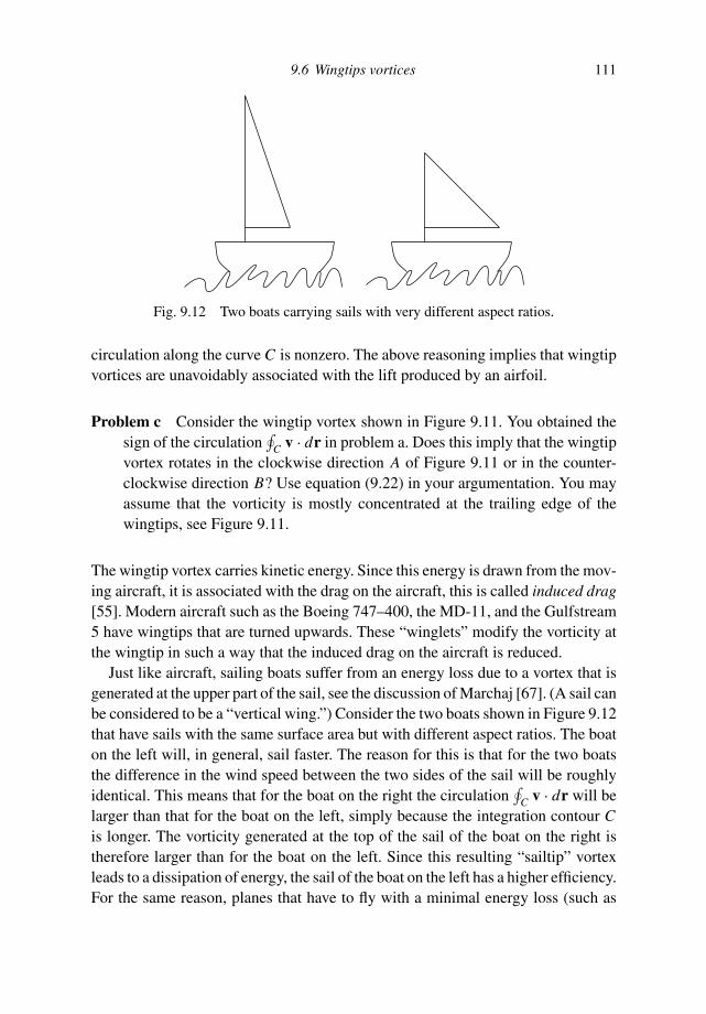
9.6 Wingtips vortices 111
Fig. 9.12 Two boats carrying sails with very different aspect ratios.
circulation along the curve C is nonzero. The above reasoning implies that wingtipvortices are unavoidably associated with the lift produced by an airfoil.
Problem c Consider the wingtip vortex shown in Figure 9.11. You obtained thesign of the circulation
∮
C v · dr in problem a. Does this imply that the wingtipvortex rotates in the clockwise direction A of Figure 9.11 or in the counter-clockwise direction B? Use equation (9.22) in your argumentation. You mayassume that the vorticity is mostly concentrated at the trailing edge of thewingtips, see Figure 9.11.
The wingtip vortex carries kinetic energy. Since this energy is drawn from the mov-ing aircraft, it is associated with the drag on the aircraft, this is called induced drag[55]. Modern aircraft such as the Boeing 747–400, the MD-11, and the Gulfstream5 have wingtips that are turned upwards. These “winglets” modify the vorticity atthe wingtip in such a way that the induced drag on the aircraft is reduced.
Just like aircraft, sailing boats suffer from an energy loss due to a vortex that isgenerated at the upper part of the sail, see the discussion of Marchaj [67]. (A sail canbe considered to be a “vertical wing.”) Consider the two boats shown in Figure 9.12that have sails with the same surface area but with different aspect ratios. The boaton the left will, in general, sail faster. The reason for this is that for the two boatsthe difference in the wind speed between the two sides of the sail will be roughlyidentical. This means that for the boat on the right the circulation
∮
C v · dr will belarger than that for the boat on the left, simply because the integration contour Cis longer. The vorticity generated at the top of the sail of the boat on the right istherefore larger than for the boat on the left. Since this resulting “sailtip” vortexleads to a dissipation of energy, the sail of the boat on the left has a higher efficiency.For the same reason, planes that have to fly with a minimal energy loss (such as

112 Theorem of Stokes
gliders) have thin and long wings. In contrast to this, planes that may waste energyin order to fly at a very high speed (such as the Concorde) have wings of a verydifferent shape. Birds follow the same rule: birds that fly relatively slowly but thatcan glide efficiently over long distances (such as the albatross) have long and thinwings, whereas birds that do not need to fly efficiently (such as a crow) have shorterand thicker wings.

10
Laplacian
The Laplacian of a function consists of a special combination of the second partialderivatives of that function. Before we introduce this quantity, the relation betweenthe second derivative and the curvature of a function is established in Section 10.1.The Laplacian is introduced in Section 10.3 using the physical example of a soapfilm that minimizes its surface area. The analysis used for this example is intro-duced in Section 10.2 where a proof is given that the shortest distance between twopoints is a straight line. The concept of the Laplacian is used in Section 10.5 tostudy the stability of matter, while in Section 10.6 the implications for the initiationof lightning is considered. Finally, the Laplacian in cylindrical and spherical coor-dinates is derived, and this is used in Section 10.8 to derive an averaging integralfor harmonic functions.
10.1 Curvature of a function
Let us consider a function f (x) that has an extremum. We are free to choose theorigin of the x-axis, and the origin is chosen here at the location of the extremum.This means that the function f (x) is stationary at the location x = 0, see Figure 10.1.The behavior of the function near its maximum can be studied using the Taylor series(3.11)
f (x) = f (0) + d f
dx(x = 0) x + 1
2
d2 f
dx2(x = 0) x2 + · · · . (3.11)
The point x = 0 is a maximum or a minimum which implies by definition that thefirst derivative vanishes at x = 0, so that the function behaves near the extremumas
f (x) = f (0) + 1
2
d2 f
dx2(x = 0) x2 + · · · . (10.1)
113

114 Laplacian
x
y
C
R
BA
y = f (x)
Fig. 10.1 Definition of the geometric variables in the computation of the radiusof curvature of a function.
When the first derivative vanishes, the function can have either a maximum or aminimum. In more dimensions, the function can have a minimum in one directionand a maximum in another direction. For this reason the terminology “extremum” isnot very accurate. Instead, one refers to a point at which the first derivative vanishesas a stationary point. This term is chosen because at such a point, the functionaccording to (10.1) does not vary to first order with the independent variable. Inmore than one dimension a stationary point is defined by the requirement that thefirst partial derivatives with respect to all variables vanish.
The property of stationary points that the first derivative vanishes correspondswith the fact that at an extremum the slope of the function vanishes. The dominantbehavior of the function near its stationary point is given by its curvature that isdescribed by the x2 term in (10.1). In order to characterize this curvature one candefine a circle as shown in Figure 10.1 that touches the function f (x) near itsextremum. This tangent-circle is shown by a dashed line in Figure 10.1. The radiusR of this circle measures the curvature of the function at its extremum. For thisreason, R is called the radius of curvature.
Problem a Convince yourself that a small radius of curvature R implies a largecurvature of f (x) and a large radius R corresponds to a small curvature off (x). What is the shape of f (x) when the radius of curvature tends to infinity(R → ∞)? Hint: draw this situation.
The radius of curvature can be determined using the points A, B, and C inFigure 10.1.
Problem b Use Figure 10.1 to show that these points have the following coordi-nates in the (x, y)-plane
rA =(
0f (0)
)
, rB =(
xf (x)
)
, rC =(
0f (0) − R
)
. (10.2)
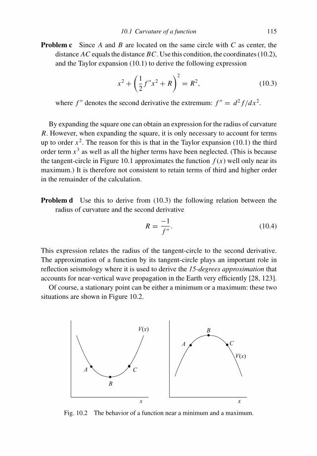
10.1 Curvature of a function 115
Problem c Since A and B are located on the same circle with C as center, thedistance AC equals the distance BC . Use this condition, the coordinates (10.2),and the Taylor expansion (10.1) to derive the following expression
x2 +(
1
2f ′′x2 + R
)2
= R2, (10.3)
where f ′′ denotes the second derivative the extremum: f ′′ = d2 f/dx2.
By expanding the square one can obtain an expression for the radius of curvatureR. However, when expanding the square, it is only necessary to account for termsup to order x2. The reason for this is that in the Taylor expansion (10.1) the thirdorder term x3 as well as all the higher terms have been neglected. (This is becausethe tangent-circle in Figure 10.1 approximates the function f (x) well only near itsmaximum.) It is therefore not consistent to retain terms of third and higher orderin the remainder of the calculation.
Problem d Use this to derive from (10.3) the following relation between theradius of curvature and the second derivative
R = −1
f ′′ . (10.4)
This expression relates the radius of the tangent-circle to the second derivative.The approximation of a function by its tangent-circle plays an important role inreflection seismology where it is used to derive the 15-degrees approximation thataccounts for near-vertical wave propagation in the Earth very efficiently [28, 123].
Of course, a stationary point can be either a minimum or a maximum: these twosituations are shown in Figure 10.2.
xx
V(x)
A
B
C
A
B
C
V(x)
Fig. 10.2 The behavior of a function near a minimum and a maximum.
116 Laplacian
Problem e Use (10.4) to show that for the curve in the left-hand panel (a mini-mum) the radius of curvature is negative and that for the curve in the right-handpanel (a maximum) the radius of curvature is positive.
The result in the last problem of course depends critically on the following propertyof a stationary point:
when f (x) is a minimum:∂2 f
∂x2> 0;
when f (x) is a maximum:∂2 f
∂x2< 0.
⎫
⎪
⎪
⎪
⎬
⎪
⎪
⎪
⎭
(10.5)
The curve in the left-hand panel of Figure 10.2 is called concave, while the curvein the right-hand panel is called convex. This implies that a concave curve has anegative radius of curvature and a convex curve has a positive radius of curvature.
The distinction between these different kinds of extrema is crucial to the stabilityproperties of physical systems. Suppose that the function denotes a potential V (x),then according to (5.31) the force associated with potential is given by
F(x) = −∇V (x). (5.31)
In one dimension this expression is given by
F(x) = − dV
dx. (10.6)
Problem f Show that at the points B in the panels of Figure 10.2 the force vanishes.
Suppose a particle that is influenced by the potential is at rest at one of the points B inFigure 10.2. Since the force vanishes at these points the particle will remain foreverat that point. For this reason the points where ∇V = 0 are called the equilibriumpoints.
However, when we move the particle slightly away from the equilibrium points,the force may either push it back towards the equilibrium point, or push it furtheraway. In the first case the equilibrium is stable, in the second case it is unstable.
Problem g Draw the direction of the force at the points A and C in the two panelsof Figure 10.2 and deduce that the equilibrium in the left-hand panel is stablewhile the equilibrium in the right-hand panel is unstable. Use (10.5) to show

10.2 Shortest distance between two points 117
that:
the equilibrium is stable when∂2V
∂x2> 0;
the equilibrium is unstable when∂2V
∂x2< 0.
⎫
⎪
⎪
⎪
⎬
⎪
⎪
⎪
⎭
(10.7)
If you find these arguments difficult, you can think of a ball that can move alongthe curves in the panels of Figure 10.2 in a gravitational field. At point B the ballis in an area that is flat. If it does not move it will remain at that point forever.When the ball in the left-hand panel moves away from the equilibrium point, itrolls uphill and the gravitational force will send it back towards the equilibriumpoint B. However, when the ball in the right-hand panel moves away from pointB, it will roll downhill further from the equilibrium point. The equilibrium at pointB in the right-hand panel is unstable. These properties are all related to the secondderivative of a function.
10.2 Shortest distance between two points
In this section we give a proof that the shortest distance between two points is astraight line. This may appear to be a trivial problem, but it is shown here becauseit sets the stage for the Laplacian. It also gives a brief introduction to variationalcalculus. This topic is treated in more detail in Chapter 25.
As an example we show that the shortest curve between two points is a straightline. The problem is shown geometrically in Figure 10.3. Two points A and B aregiven in the (x, y)-plane; these points are fixed. We are looking for the functiony = h(x) that describes the curve with the smallest length.
A
B
xx = a x = b
dxdx
dx
h(x)
dh
Fig. 10.3 The relation between the derivative of a function and the arclength ofthe corresponding curve.

118 Laplacian
A
B
x = a x = b
(x)
x
h(x)
Fig. 10.4 The unperturbed function h(x) and the perturbation ε(x) that vanishesat the endpoint of the interval.
Problem a We first need to determine the length of the curve given a certain shapeh(x). Consider an increment dx of the x-variable. Use the first-order Taylorexpansion (3.18) to show that this increment corresponds with an incrementdy = (dh/dx) dx of the y-variable. Use this result to derive that the length Lof the curve is given by:
L[h] =∫ b
a
√
1 + h2x dx, (10.8)
where hx = dh/dx .
Note that the length of the curve depends on the shape h(x) of the curve; for thisreason the notation L[h] is used.
We want to find the function h(x) that minimizes the length L . Unfortunatelywe cannot simply differentiate L with respect to h because h(x) is a functionrather than a simple variable. However, we can use the concept of stationaritythat was introduced in Section 10.1. When L[h] is minimized, the length of thecurve does not change to first order when h(x) is perturbed. Consider Figure10.4 in which a perturbation ε(x) is added to the original function h(x). Sincethe endpoints of the curve are fixed, the perturbation is required to vanish at theendpoints:
ε(a) = ε(b) = 0. (10.9)
In order to solve the problem we need to find the change δL in the length of thecurve that is caused by the perturbation ε(x).

10.2 Shortest distance between two points 119
Problem b Replace h in (10.8) by h + ε, carry out a first order Taylor expansionof the integrand with respect to ε and use this to show that the perturbation ofthe length of the curve is given by
δL[h] =∫ b
a
hxεx√
1 + h2x
dx . (10.10)
In order that the analysis is as transparent as possible we will make an approx-imation to (10.10) by restricting ourselves to the special case for which the slopeof the curve is small. Since hx = dh/dx denotes the slope of the curve, this corre-sponds to the condition hx 1. In this case the term hx in the denominator can beignored, and the perturbation is given by
δL[h] =∫ b
ahxεx dx . (10.11)
We show in Section 25.3 that the results of this Section 10.2 also hold when theapproximation hx 1 is not used; the only reason for making the approximation isthat we do not want the principle of variational calculus to be hidden by analyticalcomplexity.
Expression (10.11) gives the first order perturbation of the length with respect toε(x). The condition of stationarity tells us that for the shortest curve, (10.11) mustbe equal to zero for any small perturbation ε(x). However, we have not yet usedthe constraint (10.9) which states that the endpoints of the curve are fixed.
Problem c Carry out an integration by parts of (10.11) and use the constraint(10.9) to show that the first order perturbation is given by
δL[h] = −∫ b
a
d2h
dx2ε dx . (10.12)
For the function h(x) that minimizes the length of the curve this integral must vanishfor all perturbations ε(x). This is the case when
d2h
dx2= 0. (10.13)
This expression states that the curve that has the smallest length has no curvature,and it therefore a straight line.
Problem d Let the y-coordinates of the points A and B be denoted by yA andyB respectively. Integrate (10.13) subject to the condition that the curve goes
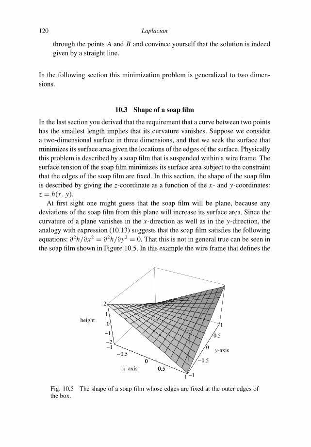
120 Laplacian
through the points A and B and convince yourself that the solution is indeedgiven by a straight line.
In the following section this minimization problem is generalized to two dimen-sions.
10.3 Shape of a soap film
In the last section you derived that the requirement that a curve between two pointshas the smallest length implies that its curvature vanishes. Suppose we considera two-dimensional surface in three dimensions, and that we seek the surface thatminimizes its surface area given the locations of the edges of the surface. Physicallythis problem is described by a soap film that is suspended within a wire frame. Thesurface tension of the soap film minimizes its surface area subject to the constraintthat the edges of the soap film are fixed. In this section, the shape of the soap filmis described by giving the z-coordinate as a function of the x- and y-coordinates:z = h(x, y).
At first sight one might guess that the soap film will be plane, because anydeviations of the soap film from this plane will increase its surface area. Since thecurvature of a plane vanishes in the x-direction as well as in the y-direction, theanalogy with expression (10.13) suggests that the soap film satisfies the followingequations: ∂2h/∂x2 = ∂2h/∂y2 = 0. That this is not in general true can be seen inthe soap film shown in Figure 10.5. In this example the wire frame that defines the
−1−0.5
00.5
1
-axis−1
−0.5
0
0.5
1
y-axis
−2
−1
0
1
2
height
00.5x -
Fig. 10.5 The shape of a soap film whose edges are fixed at the outer edges ofthe box.

10.3 Shape of a soap film 121
edge of the soap film is not confined to a plane. This results in a soap film that iscurved and hence it is not possible that both ∂2h/∂x2 and ∂2h/∂y2 are equal tozero. In this section we derive an equation for the shape of the soap film.
The position of a point on the soap film is given by the following position vector:
r =⎛
⎝
xy
h(x, y)
⎞
⎠ . (10.14)
In problem e of Section 4.4 you showed that the surface area d S of a sphere thatcorresponds to increments dθ and dϕ of the angles on the sphere is given by
d S =∣
∣
∣
∣
∂r∂θ
× ∂r∂ϕ
∣
∣
∣
∣
dθdϕ. (4.34)
Problem a Use the reasoning used in problem e of Section 4.4 to show thatincrements of the surface area of the soap film satisfy the following expression
d S =∣
∣
∣
∣
∂r∂x
× ∂r∂y
∣
∣
∣
∣
dxdy. (10.15)
Problem b Use (10.14) and (10.15) to derive that the total surface area is givenby
S =∫∫ √
1 + |∇h|2 dxdy. (10.16)
Note the analogy between this expression and (10.8).
Since the surface tension that governs the shape of the soap film tends to minimizethe surface area of the soap film, the shape h(x, y) follows from the requirement thath(x, y) is the function that minimizes the surface area (10.16). As in Section 10.2 thesolution follows from the requirement that for the function h(x, y) that minimizesthe surface area, the surface area is stationary for perturbations of h(x, y). Thismeans that when h(x, y) is replaced by h(x, y) + ε(x, y) the first order change ofthe surface area S vanishes.
Problem c Make the substitution h(x, y) → h(x, y) + ε(x, y), use the identity|∇h|2 = (∇h · ∇h) in (10.16) and linearize the result in ε(x, y) to derive thatthe perturbation of the surface area is to first order in ε(x, y) given by
δS[h] =∫∫
(∇h · ∇ε)√
1 + |∇h|2dxdy. (10.17)
122 Laplacian
In order to concentrate on the essentials we assume that the deflection of the soapsurface is small, which means that |∇h| 1. Under this assumption the |∇h| termin the denominator can be ignored and the perturbation is given by
δS[h] =∫∫
(∇h · ∇ε) dxdy. (10.18)
In the problem we are considering here, the edge of the soap film is kept at afixed location. This means that the perturbation ε(x, y) must vanish at the edge ofthe soap film:
ε(x, y) = 0 at the edge of the soap film. (10.19)
This constraint has not yet been taken into account; it is incorporated in the followingtwo problems.
Problem d Derive the identity (∇h · ∇ε) = ∇ · (ε∇h) − ε∇ · ∇h.
Problem e Insert this result in (10.18), apply Gauss’s theorem to the first term,and use (10.19) to show that the resulting integral over the edge of the surfacevanishes, so that the perturbation of the surface area is given by
δS[h] = −∫∫
ε (∇ · ∇h) dxdy. (10.20)
The second derivative (∇ · ∇h) is called the Laplacian of h. This operator isoften denoted by the notation . However, since the term ∇ · ∇ is reminiscent ofthe square of the vector ∇, the notation ∇2 is also used, and in this book this latternotation is the one we will mostly use for the Laplacian. The requirement that thefirst order perturbation of the soap film vanishes implies that (∇ · ∇h) must be equalto zero. The soap film therefore satisfies the following differential equation:
∇2h = 0. (10.21)
In mathematical physics this equation is called the Laplace equation. Before ana-lyzing this equation in more detail we first define the Laplacian more precisely.
Problem f Use the definition ∇2 = ∇ · ∇ to show that
∇2 = div grad = ∂2
∂x2+ ∂2
∂y2(in two dimensions) . (10.22)

10.3 Shape of a soap film 123
−1−0.5
0
0.5
1 −1
−0.5
0
0.5
1
y-axis
−1−0.5
00.5
1
height
0
0.5x-axis
Fig. 10.6 The shape of the same soap film as in the previous figure after a rotationthrough 45 degrees. (New edges define the area of this soap film.) The shape of thesoap film is given by the function h(x, y) = x2 − y2; the shape of the soap film inthe previous figure is given by h(x, y) = 2xy.
Analogously the Laplacian in three dimensions is defined as
∇2 = div grad = ∂2
∂x2+ ∂2
∂y2+ ∂2
∂z2(in three dimensions) . (10.23)
Let us now consider the shape of the soap film that is shown in Figure 10.5.At the beginning of this section it was argued that the curvatures ∂2h/∂x2 and∂2h/∂y2 of the soap film in the x- and y-directions could not both be equal to zero.Instead, (10.21) implies that the sum of the curvatures in the x- and y-directionsvanishes. This can be seen by rotating the soap film through 45 degrees as shownin Figure 10.6.
Problem g Sketch cross sections of the surface in Figure 10.6 along the x- and y-axes, and show that for that surface the curvature in the x-direction is positiveand the curvature in the y-direction is negative.
Problem h The surface in Figure 10.6 is given by
h(x, y) = x2 − y2. (10.24)
Show that for this surface ∇2h = 0 and that the curvatures in the x-directionand in the y-direction cancel.
These results imply that the soap film behaves in a fundamentally different waythan the rubber band between two fixed points that we treated in the previous

124 Laplacian
section. The rubber band follows a straight line and the curvature is equal to zerowhile for the soap film the sum of the curvatures in orthogonal directions vanishes.However, as shown in Figures 10.5 and 10.6 this does not imply that the soap filmis a planar surface. The fact that the curvature terms ∂2h/∂x2 and ∂2h/∂y2 haveopposite signs implies that when the function is concave in one direction it mustbe convex in the other direction. This means that when the function is a maximumin one direction, it must be a minimum in the other direction. The surface thereforehas the shape of saddle.
Let us now consider a stationary point of the function: that is a point where∂h/∂x = ∂h/∂y = 0. This point can be neither a minimum nor a maximum becausewhen it is a minimum for variations in one direction, it must be a maximum forvariations in the other direction. This means that:
Theorem A function that satisfies∇2h = 0 cannot have an extremum; the functioncan only have a maximum or minimum at the edge of the domain on which itis defined.
We will see in Section 10.5 that this has important consequences. When a function isa minimum all the second derivatives must analogously to (10.5) be positive, whilefor an extremum that is a maximum all the second derivatives must be negative.
Problem i Show that:
when h(r) is a minimum: ∇2h > 0;
when h(r) is a maximum: ∇2h < 0.
⎫
⎬
⎭
(10.25)
Problem j The above condition is a necessary but not a sufficient condition.(This means that every minimum must satisfy the requirement ∇2h > 0,but conversely when ∇2h > 0 is satisfied the function is not necessarilya minimum.) Show this by analyzing the stationary point of the functionh(x, y, z) = x2 + y2 − z2.
10.4 Sources of curvature
The main point of the previous section is that a function that satisfies the Laplaceequation (10.21) can have nonzero curvature. In general there are two reasons whya soap film can be curved. The first reason is that the edges of the soap film are notconfined to a common plane, as shown in Figures 10.5 and 10.6. Since the edges arepart of the soap film, this necessarily implies that the soap film cannot be confinedto a plane.

10.4 Sources of curvature 125
There is another reason why a soap film can be curved. Let us consider a soapfilm whose edges are located in the (x, y)-plane:
h(x, y) = 0 at the edge. (10.26)
However, let us suppose that gravity pulls the soap film down. Such a soap filmwill bend down from the edges and will therefore be curved. This means that anexternal force can also lead to curvature of the soap film.
In this section we derive the differential equation for a soap film that is subjectto a gravitational force. This is achieved by minimizing the total energy of the soapfilm. The gravitational energy is given by ρgh, where ρ is the mass-density perunit area and g is the acceleration of gravity. The surface energy of the soap film issome positive constant k times the surface area of the soap film.
Problem a Use these results and (10.16) to show that the total energy is given by:
E =∫∫ (
k√
1 + |∇h|2 + ρgh
)
dxdy. (10.27)
The shape of the soap film is determined by the condition that the energy is aminimum.
Problem b In the previous section we minimized the first term in the integrand.Generalize the derivation of the previous section to take the second term in(10.27) into account as well to derive that the soap film under gravity satisfiesthe following differential equation:
∇2h = ρg
k. (10.28)
This equation is called Poisson’s equation. The gravitational force has the effectthat the total curvature of the soap film can be nonzero. This corresponds to thereasoning at the beginning of this section that gravity will make the soap film sag,so that the total curvature can be nonzero despite the fact that the edges of the soapfilm are confined to a plane. Note that gravity acts as a source term in the differentialequation (10.28).
There is an interesting analogy between the soap film in a gravitational field andthe electric potential that is generated by electric charges. According to equation(6.23) the electric field generated by a charge density ρ is given by
(∇ · E) =ρ(r)/ε0. (6.23)
By analogy with (5.31) the potential associated with this electric field is given by
E = −∇V . (10.29)
126 Laplacian
Problem c Show that the potential satisfies
∇2V = −ρ/ε0. (10.30)
This means that the electric potential satisfies Poisson’s equation (10.28) as well.The electric charge acts as the source of the electric potential just as the gravitationalforce acts as the source of the deflection of the soap film.
The analogy between the deflection of the soap film and the electric potential isinteresting. Let us consider once more a soap film that is not subject to a gravita-tional force. The equation (10.28) of the soap film followed from the requirementthat the squared-gradient |∇h|2 integrated over the surface was minimized, be-cause then the term
√1 + |∇h|2 in (10.16) is minimized as well. The analogy
with the electric potential means that in free space (ρ = 0) the electric potentialbehaves in such a way that the squared-gradient |∇V |2of the potential integratedover the volume is minimized. However, according to (10.29) the gradient of theelectric potential is the electric field. This means that the electric field behaves insuch a way that the volume integral
∫ |E|2 d3x is minimized. However, this quan-tity is nothing but the energy of a static electric field [53]. This implies that theelectric field is distributed in such a way that the energy of the electric field isminimized.
10.5 Instability of matter
The title of this section may surprise you, but the results that will be obtained hereimply that according to the laws of classical physics the structure of matter and themass distribution in the universe cannot be in a stable equilibrium. This result wasderived by Earnshaw in 1842 in his work “On the nature of the molecular forceswhich regulate the constitution of the luminiferous ether” [36]. Let us consider aparticle in three dimensions that is subject to a potential V (r) that accounts forthe gravitational attraction by other masses and the electrostatic force due to othercharges. Let us suppose that at some point in space the particle is in equilibrium.This means that the force acting on the particle vanishes at that point, or equivalentlythat the gradient of the potential vanishes at that point: ∇V = 0.
Problem a Generalize expression (10.7) to three dimensions to show that thisequilibrium point is only stable when the curvature of the potential in the threecoordinate directions is positive:
∂2V
∂x2> 0 and
∂2V
∂y2> 0 and
∂2V
∂z2> 0. (10.31)
10.5 Instability of matter 127
According to (10.30), in free space (ρ = 0) the potential that corresponds to thegravitational force exerted by other masses, and the electrostatic force generatedby other charges, satisfies Laplace’s equation ∇2V = 0.
Problem b Show that Laplace’s equation implies that when the curvature of thepotential is positive in one direction, the curvature must be negative in at leastone other direction.
Problem c Use this to deduce that when the equilibrium point is stable to pertur-bations in one direction, it must be unstable for perturbations in at least oneother direction.
An equilibrium point is in general unstable when it is unstable for perturba-tions in at least one of the directions. Using problem c this means that an equi-librium point for the potential V (r) that satisfies Poisson’s equation cannot bestable.
This has far-reaching consequences. Let us consider a crystal. Within the frame-work of classical physics, each ion in the crystal moves in an electric potential thatis generated by all the other ions in the crystal. This potential satisfies Laplace’sequation at the location of the ion that we are considering because the net chargedensity ρ of the other ions is zero at that point. This means that the motion of theion at its equilibrium point is not stable. When this is the case, the crystal is notstable because small perturbations of each ion from its equilibrium point lead tounstable motions of the ions. This implies that according to the laws of classicalphysics, matter is not stable! This result, known as Earnshaw’s theorem [36], statesthat the equilibrium points of any configuration of static electrical, magnetic, andgravitational fields are unstable.
Hopefully you are convinced that matter is stable, whatever the unsettling predic-tion of Earnshaw’s theorem may be. The only way that we can resolve this paradoxis if matter does not satisfy the equations of classical mechanics and electrostat-ics. This implies that quantum effects must play a crucial role in the stability ofmatter.
Earnshaw’s theorem also applies to the gravitational field and it states that equi-librium points in the gravitational field are not stable. This means that a universe inequilibrium would not be stable! Let us first consider our solar system. It is essentialfor the solar system that the planets and their moons are in motion. This means thatthe solar system is not in a static equilibrium. In fact, the motion of the planets andmoons is governed by the combination of the gravitational force plus the inertiaforce that is associated with the motion of the planets. The miracle of planetarymotion is that the gravitational motion is stable. (You showed in Section 6.5 that

128 Laplacian
the motion of planetary orbits is only stable in less than four spatial dimensions.)The situation is comparable to the movement of a bicycle which derives its stabilityfrom the motion of the wheels that rotate. In the same way, it is the combinationof the gravitational field and the inertial forces due to the motion of the planetsthat leads to stable planetary orbits. On scales much larger than the solar system,relativistic effects are important and Poisson’s equation is not sufficient to describethe gravitational field on a cosmological scale [76].
In 1842, Earnshaw [36] carried out his work not to study the structure of matter,but to study the structure of the ether, which at that time was seen as the carrierof electromagnetic waves. He viewed the ether as a system of interacting particlesand showed that the interaction between these particles could not be governedby Newton’s law of gravitation using the analysis shown in this section. Fromthe requirement of stability he derived conditions for the potential that governsthe interaction between etheral particles. Note that in 1842 Earnshaw could notinvoke quantum mechanics in his description of interacting microscopic particlesbecause that theory had not yet been formulated.
10.6 Where does lightning start?
During a thunderstorm, the vertical motion of ice particles causes the separationof positive and negative electric charges in the atmosphere. This charge separationleads to an electric field within the atmosphere. When the field strength at a certainlocation is sufficiently strong, atoms are ionized and a current flows. This currentinduces further ionization which extends the path of the current. This physicalprocess describes the events that initiate a lightning bolt. In principle there seemsto be no reason why a lightning bolt cannot start in mid-air, far away from theEarth’s surface and far from the electrical charges that induce the electric field. Inthis section we show that lightning can only start at specific locations.
To see this we study the Laplacian of the square of the length of a vector field E.
Problem a Compute the Laplacian of E2 = E2x + E2
y + E2z and show that it is
given by
∇2 E2 = 2(
|∇Ex |2 + ∣
∣∇Ey
∣
∣
2 + |∇Ez|2)
+ 2(
E · ∇2E)
. (10.32)
(Up to this point the Laplacian has always acted on a scalar; when it acts on avector as in (10.32) it means that the Laplacian of every component is takenso that ∇2E stands for a vector with components ∇2 Ex , ∇2 Ey and ∇2 Ez ,respectively.)

10.7 Laplacian in spherical and cylindrical coordinates 129
Let us now consider a vector field E that satisfies the Laplace equation:
∇2E = 0. (10.33)
Problem b Show that a vector field that satisfies the Laplace equation (10.33)satisfies the following inequality:
∇2 E2 ≥ 0. (10.34)
Problem c Use this to show that the strength of the vector field (E2) cannot havea maximum in the region where (10.33) is satisfied.
Note that (10.34) does not exclude the possibility that E2 has a minimum.The result you derived in problem c is all we need to solve our problem.
Away from the charges in the atmosphere, a static electric field satisfies (10.33),see reference [53]. According to problem c, the electric field strength E2 can-not have a maximum in the region of the atmosphere where there are no chargesthat are the source of the field. Lightning will initiate where the field strengthis strongest. This means that lightning must initiate either in the regions whereLaplace equation (10.33) does not hold (at the charges that generate the elec-tric field), or at the boundary of the area (the Earth’s surface). This implies thatlighting must start either at the charges that generate the field or at the Earth’ssurface.
Problem d The source of the magnetic field of the Earth is located in the Earth’score. Away from this source, the magnetic field satisfies Laplace equation(10.33) (at least when the field is stationary)[53]. Show that the magnetic fieldof the Earth cannot have its maximum strength outside the Earth.
10.7 Laplacian in spherical and cylindrical coordinates
In many applications it is useful to use the Laplacian in spherical or cylindrical coor-dinates. In principle this result can be derived by applying the transformation rulesto the second partial derivatives in the Laplacian when changing from Cartesian tospherical or cylindrical coordinates. However, this route is unnecessarily complex,especially since we have done most of the work already. The key element in thederivation was derived in problem f of Section 10.3 where you showed that theLaplacian is the divergence of the gradient: ∇2 = div grad. In Sections 5.6 and 6.4you have already derived expressions for the gradient and the divergence in spher-ical and cylindrical coordinates, and all you need to do is to insert the expression
130 Laplacian
for the gradient in curvilinear coordinates into the expression of the divergence incurvilinear coordinates.
Problem a Use (5.48) and (6.31) to show that the Laplacian of a function f incylindrical coordinates is given by
∇2 f = 1
r
∂
∂r
(
r∂ f
∂r
)
+ 1
r2
∂2 f
∂ϕ2+ ∂2 f
∂z2. (10.35)
Problem b Find the expressions in Sections 5.6 and 6.4 that allow you to derivethat the Laplacian of a function f in spherical coordinates is given by
∇2 f = 1
r2
∂
∂r
(
r2 ∂ f
∂r
)
+ 1
r2 sin θ
∂
∂θ
(
sin θ∂ f
∂θ
)
+ 1
r2 sin2 θ
∂2 f
∂ϕ2. (10.36)
In later parts of this book extensive use is made of these expressions of the Laplacian.
10.8 Averaging integrals for harmonic functions
In this section we focus on functions f that satisfy Laplace’s equation (10.21),that is ∇2 f = 0. Functions whose Laplacian is zero are called harmonic functions.They play an important role in mathematical physics. We will show in Section16.1 that the real and imaginary parts of analytic functions in the complex planeare harmonic functions. Let us first focus on a harmonic function f (x, y) in twodimensions. In this section we derive that the function value at a certain point isequal to the average of that function over a circle centered around that point with anarbitrary radius. To see this we use a system of cylindrical coordinates and choosethe origin of the cylindrical coordinates at the point that we consider. (Rememberthat we are free to choose the origin of the coordinate system.)
Problem a Use expression (10.35) to show that f satisfies the following differ-ential equation:
1
r
∂
∂r
(
r∂ f
∂r
)
+ 1
r2
∂2 f
∂ϕ2= 0. (10.37)
Problem b Integrate this expression over a disk of radius R centered at the originand derive that
∫ R
0
∫ 2π
0
[
∂
∂r
(
r∂ f
∂r
)
+ 1
r
∂2 f
∂ϕ2
]
dϕdr = 0. (10.38)
(Note the powers of r in this expression.)

10.8 Averaging integrals for harmonic functions 131
Problem c Carry out the ϕ-integration in the last term of the integrand to showthat this term gives a vanishing contribution.
It is convenient to introduce at this point the average f (r ) of the function f overa circle with radius r :
f (r ) ≡ 1
2π
∫ 2π
0f (r, ϕ) dϕ. (10.39)
Problem d Use (10.38) and the result of problem c to derive that f satisfies thefollowing equation:
[
r∂ f
∂r
]r=R
r=0
= 0. (10.40)
Problem e This expression holds for any radius R, hence r∂ f /∂r is independentof r , so that it is a constant: r∂ f /∂r = C . Integrate this expression to derivethat
f (r ) = C ln r + A, (10.41)
where A is an unknown integration constant.
Problem f The integration constant C must be equal to zero because f (r ) is finiteas r → 0. Evaluate (10.41) at the origin, determine the constant A and showthat f (r ) satisfies
f (r = 0) = 1
2π
∫ 2π
0f (r, ϕ) dϕ. (10.42)
This expression states that the value of a harmonic function at the origin is theaverage of the function over a circle with arbitrary radius. The amazing propertyis that this holds for any value of the radius, provided f is harmonic everywherewithin the circle with radius r . Note that we are free to choose the origin of thecoordinate system so that the averaging integral (10.42) holds for any point.
The averaging integral can also be used to prove that a harmonic function cannothave a minimum or a maximum in the region where it is defined. Suppose thefunction had a maximum at a certain location. There then exists a circle aroundthis point where the function has smaller values than at the maximum (otherwise itwould not be a maximum). Equation (10.42) cannot hold for this circle because theright-hand side would be smaller than the left-hand side. Therefore it is impossiblefor f to have a maximum.

132 Laplacian
Problem g Generalize the derivation in this section to spherical coordinates andderive the following expression for harmonic functions in three dimensions
f (r = 0) = 1
4π
∫ π
0
∫ 2π
0f (r, θ, ϕ) sin θ dϕdθ. (10.43)
Problem h Show that the right-hand side of this expression is the average of thatfunction over a sphere with arbitrary radius r centered around that point r = 0.
This means that, in three dimensions, the value of a harmonic function at a certainpoint is equal to the average of the function over a sphere with arbitrary radius rthat is centered on that point.
11
Conservation laws
In physics one frequently handles the change of a property with time by consideringproperties that do not change with time. For example, when two particles collideelastically, the momentum and the energy of each particle may change. However,this change can be found from the consideration that the total momentum and energyof the system are conserved. Often in physics, such conservation laws are the mainingredients for describing a system. In this chapter we deal with conservation lawsfor continuous systems. These are systems in which the physical properties are acontinuous function of the space coordinates. Examples are the motion in a fluid orsolid, and the temperature distribution in a body. The introduced conservation lawsare not only of great importance in physics, they also provide worthwhile exercisesin the use of vector calculus introduced in the previous chapters.
11.1 General form of conservation laws
In this section a general derivation of conservation laws is given. Suppose weconsider a physical quantity Q. This quantity could denote the mass density of afluid, the heat content within a solid or any other type of physical variable. In fact,there is no reason why Q should be a scalar, it could also be a vector (such asthe momentum density) or a higher order tensor. Let us consider a volume V inspace that does not change with time. This volume is bounded by a surface ∂V .The total amount of Q within this volume is given by the integral
∫
V QdV . Therate of change of this quantity with time is given by (∂/∂t)
∫
V QdV .In general, there are two reasons for the quantity
∫
V QdV to change with time.First, the field Q may have sources or sinks within the volume V . The net source ofthe field Q per unit volume is denoted by the symbol S. The total source of Q withinthe volume is simply the volume integral
∫
V SdV of the source density. Second, itmay be that the quantity Q is transported in the medium. With this transport processis associated a current J of the quantity Q. As an example one can think of Q as
133
134 Conservation laws
being the mass-density of a fluid. In that case∫
V QdV is the total mass of the fluidin the volume. This total mass can change because there is a source of fluid withinthe volume (i.e. a tap or a bathroom sink), or the total mass may change because ofthe flow through the boundary of the volume.
The rate of change of∫
V QdV by the current is given by the inward flux ofthe current J through the surface ∂V . If we retain the convention that the surfaceelement dS points out of the volume, the inward flux is given by − ∮
∂V J · dS.Together with the rate of change due to the source density S within the volume thisimplies that the rate of change of the total amount of Q within the volume satisfies:
∂
∂t
∫
VQdV = −
∮
∂VJ · dS +
∫
VSdV . (11.1)
Using Gauss’s law (8.1), the surface integral on the right-hand side can be writtenas − ∫
V (∇ · J)dV , so that the expression above is equivalent with
∂
∂t
∫
VQdV +
∫
V(∇ · J)dV =
∫
VSdV . (11.2)
Since the volume V is assumed to be fixed with time, the time-derivativeof the volume integral is the volume integral of the time-derivative:(∂/∂t)
∫
V QdV = ∫
V (∂ Q/∂t)dV . It should be noted that (11.2) holds for any vol-ume V . If the volume is an infinitesimal volume, the volume integrals in (11.2) canbe replaced by the integrand multiplied by the infinitesimal volume. This meansthat (11.2) is equivalent to:
∂ Q
∂t+ (∇ · J) = S. (11.3)
This is the general form of a conservation law in physics; it simply states that therate of change of a quantity is due to the sources (or sinks) of that quantity and dueto the divergence of the current of that quantity. Of course, the general conservationlaw (11.3) is not very meaningful as long as we do not provide expressions for thecurrent J and the source S. In this section we will see some examples in whichthe current and the source follow from physical theory, but we will also encounterexamples in which they follow from an “educated” guess.
Equation (11.3) will not be completely new to you. In Section 8.4 the probability-density current for a quantum-mechanical system was derived.
Problem a Use the derivation in this section to show that expression (8.16) canbe written as
∂
∂t|ψ |2 + (∇ · J) = 0, (11.4)
with J given by (8.18).
11.2 Continuity equation 135
This equation constitutes a conservation law for the probability density of a quantumparticle. Note that (8.16) could be derived rigorously from the Schrodinger equation(8.14), so that the conservation law (11.4) and the expression for the current J followfrom the basic equation of the system.
Problem b Why is the source term on the right-hand side of (11.4) equal to zero?
11.2 Continuity equation
In this section we consider the conservation of mass in a continuous medium suchas a fluid or a solid. In that case, the quantity Q is the mass-density ρ. If we assumethat mass is neither created nor destroyed, the source term vanishes: S = 0. Thevector J is the mass current and denotes the flow of mass per unit volume. Considera small volume δV . The mass within this volume is equal to ρδV . If the velocityof the medium is denoted by v, the mass flow is given by ρδV v. Dividing this bythe volume δV one obtains the mass flow per unit volume; this quantity is calledthe mass-density current:
J = ρv. (11.5)
Using these results, the principle of the conservation of mass can be expressed as
∂ρ
∂t+ ∇ · (ρv) = 0. (11.6)
This expression plays an important role in continuum mechanics, and is called thecontinuity equation.
Up to this point the reasoning has been based on a volume V that did not changewith time. This means that our treatment was strictly Eulerian: we considered thechange of physical properties at a fixed location. As an alternative, a Lagrangiandescription of the same process can be given. In such an approach one specifies howphysical properties change as they are moved along by the flow. In this approachone seeks an expression for the total time-derivative d/dt of physical propertiesrather than expressions for the partial derivative ∂/∂t . It follows from (5.40) thatthese two derivatives are related in the following way:
d
dt= ∂
∂t+ (v · ∇). (11.7)
This distinction between the total time-derivative and the partial time-derivative istreated in detail in Section 5.5.
Problem a Show that the total derivative of the mass-density is given by:
dρ
dt+ ρ(∇ · v) = 0. (11.8)
136 Conservation laws
Problem b This expression gives the change in the density when one follows theflow. Let us consider an infinitesimal volume δV that is carried around withthe flow. The mass of this volume is given by δm = ρδV . The volume moveswith the flow, therefore there is no mass transport across the boundary of thevolume. This means that the mass within that volume is conserved: δm = 0.The dot denotes the total time-derivative, not the partial time-derivative. Usethis expression and (11.8) to show that (∇ · v) is the rate of change of thevolume normalized by size of the volume:
δV
δV= (∇ · v). (11.9)
We have learned a new meaning of the divergence of the velocity field: itequals the relative change in volume per unit time.
11.3 Conservation of momentum and energy
In the description of a point mass in classical mechanics, the conservation of mo-mentum and energy can be derived from Newton’s third law. The same is true for acontinuous medium such as a fluid or a solid. In order to formulate Newton’s law fora continuous medium we start with a Lagrangian point of view and consider a vol-ume δV that moves with the flow. The mass of this volume is given by δm = ρδV .This mass is constant because the volume is defined to move with the flow, hencemass cannot flow into or out of the volume. Let the force per unit volume be denotedby F, so that the total force acting on the volume is FδV . The force F contains bothforces generated by external agents (such as gravity) and internal agents such as thepressure force −∇ p or the effect of internal stresses (∇ · σ). The stress tensor σ istreated in Section 22.10. Newton’s law applied to the volume δV takes the form:
d
dt(ρδV v) = FδV . (11.10)
Since the mass δm = ρδV is constant with time it can be taken outside the derivativein (11.10). Dividing the resulting expression by δV leads to the Lagrangian formof the equation of motion:
ρdvdt
= F. (11.11)
Note that the density appears outside the time-derivative, despite the fact that thedensity may vary with time. Using the prescription (11.7) one obtains the Eulerianform of Newton’s law for a continuous medium:
ρ∂v∂t
+ ρv · ∇v = F. (11.12)
11.3 Conservation of momentum and energy 137
This equation is not yet in the general form (11.3) of conservation laws because inthe first term on the left-hand side we have the density times a time-derivative, andbecause the second term on the left-hand side is not the divergence of some current.
Problem a Use (11.12) and the continuity equation (11.6) to show that:
∂(ρv)
∂t+ ∇ · (ρvv) = F. (11.13)
This expression does take the form of a conservation law; it expresses that themomentum (density) ρv is conserved. (For brevity we will often not include theaffix “density” in the description of the different quantities, but remember that allquantities are given per unit volume.) The source of momentum is given by the forceF, and this reflects that forces are the cause of changes in momentum. In additionthere is a momentum current J = ρvv that describes the transport of momentumby the flow. This momentum current is not a simple vector, it is a dyad and henceis represented by a 3 × 3 matrix. This is not surprising since the momentum isa vector with three components and each component can be transported in threespatial directions.
Sometimes there is a certain arbitrariness in what we call the current and whatwe call the source. As an example let us consider (11.13) again. According to (5.12)the pressure force is given by F = −∇ p. If there are no other forces acting on thefluid, the right-hand side of (11.13) is given by −∇ p. This term does not have theform of the divergence, but we can rewrite it by using that:
∂p
∂xi=
∑
j
∂
∂x j
(
pδi j)
, (11.14)
where δi j is the Kronecker delta. This quantity is defined as follows:
δi j =
1 when i = j0 when i = j
. (11.15)
The matrix elements of the identity matrix I are given by the Kronecker delta:Ii j = δi j .
Problem b Show that expression (11.14) may be written in vector form as ∇ p =∇ · (pI). Show that the law of conservation of momentum is given by
∂(ρv)
∂t+ ∇ · S = 0, (11.16)
where S is defined by
S =ρvv + pI. (11.17)
138 Conservation laws
This quantity describes the radiation stress [10] which accounts for the internalstress in an acoustic medium that is generated by the waves that propagate throughthe medium. Of course, when other external forces are present, they will lead toa right-hand side of (11.16) that is nonzero. This example shows that it can bearbitrary whether a certain physical effect is accounted for by a source term orby a current. This arbitrariness is caused by the fact that it is not clear what isinternal to the system and what is external. In (11.13) the pressure force is treatedas an external force whereas in (11.17) the pressure contributes to a current withinthe system. There is no objective reason to prefer one or the other of the twoformulations.
You may find the inner products of vectors and the ∇-operator in expressionssuch as (11.12) confusing, and indeed a notation such as ρv · ∇v can be a source oferror and confusion. When working with quantities like this it is clearer to explicitlywrite out the components of all vectors or tensors. In component form an equationsuch as (11.12) is written as:
ρ∂vi
∂t+
∑
j
ρv j∂ jvi = Fi . (11.18)
Problem c Rewrite the continuity equation (11.6) in component form and redothe derivation of problem a with all equations in component form to arrive atthe conservation law of momentum in component form:
∂(ρvi )
∂t+
∑
j
∂ j (ρv jvi ) = Fi . (11.19)
In order to derive the law of energy conservation we start by deriving the con-servation law for the kinetic energy (density)
EK = 1
2ρv2 =
∑
i
1
2ρvivi . (11.20)
Problem d Express the partial time-derivative ∂(ρv2)/∂t in the time-derivatives∂(ρvi )/∂t and ∂vi/∂t , use (11.18) and (11.19) to eliminate these time-derivatives and write the final results as:
∑
i
∂( 12ρvivi )
∂t= −
∑
i, j
∂ j
(
1
2ρviviv j
)
+∑
j
v j Fj . (11.21)

11.3 Conservation of momentum and energy 139
Problem e Use definition (11.20) to rewrite the expression above as the conser-vation law of kinetic energy:
∂ EK
∂t+ ∇ · (vEK ) = (v · F). (11.22)
This equation states that the kinetic energy current is given by J = vEK , and thisterm describes how kinetic energy is transported by the flow. The term (v · F) onthe right-hand side denotes the source of kinetic energy. It was shown in Section5.4 that (v · F) is the power delivered by the force F. This means that (11.22) statesthat the power produced by the force F is the source of kinetic energy.
In order to invoke the potential energy as well we assume for the moment thatthe force F is the gravitational force. Suppose there is a gravitational potential V (r),then the gravitational force is given by
F = − ρ∇V, (11.23)
and the potential energy EP is given by
EP = ρV . (11.24)
Problem f Take the (partial) time-derivative of (11.24), use the continuity equa-tion (11.6) to eliminate ∂ρ/∂t , use that the potential V does not depend ex-plicitly on time, and employ (11.23) and (11.24) to derive the conservationlaw of potential energy:
∂ EP
∂t+ ∇ · (vEP ) = −(v · F). (11.25)
Note that this conservation law is very similar to the conservation law (11.22) forkinetic energy. The meaning of the second term on the left-hand side will be clearto you by now; it denotes the divergence of the current vEP of potential energy.Note that the right-hand side of (11.24) has the opposite sign to the right-handside of (11.22). This reflects the fact that when the force F acts as a source ofkinetic energy, it acts as a sink of potential energy; the opposite signs imply thatkinetic and potential energy are converted into each other. However, the total energyE = EK + EP should have no source or sink.
Problem g Show that the total energy is source-free:
∂ E
∂t+ ∇ · (vE) = 0. (11.26)
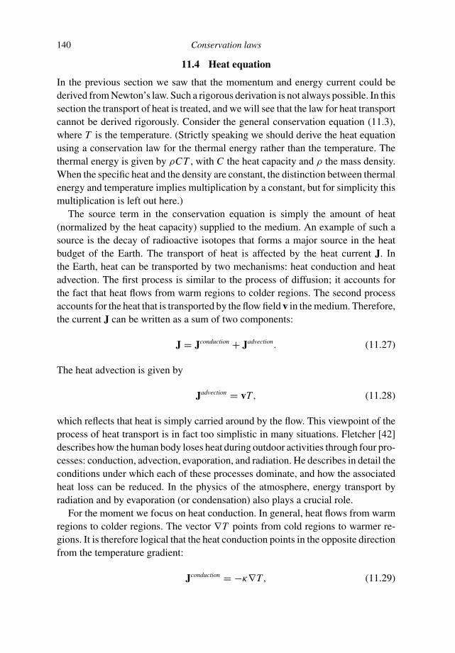
140 Conservation laws
11.4 Heat equation
In the previous section we saw that the momentum and energy current could bederived from Newton’s law. Such a rigorous derivation is not always possible. In thissection the transport of heat is treated, and we will see that the law for heat transportcannot be derived rigorously. Consider the general conservation equation (11.3),where T is the temperature. (Strictly speaking we should derive the heat equationusing a conservation law for the thermal energy rather than the temperature. Thethermal energy is given by ρCT , with C the heat capacity and ρ the mass density.When the specific heat and the density are constant, the distinction between thermalenergy and temperature implies multiplication by a constant, but for simplicity thismultiplication is left out here.)
The source term in the conservation equation is simply the amount of heat(normalized by the heat capacity) supplied to the medium. An example of such asource is the decay of radioactive isotopes that forms a major source in the heatbudget of the Earth. The transport of heat is affected by the heat current J. Inthe Earth, heat can be transported by two mechanisms: heat conduction and heatadvection. The first process is similar to the process of diffusion; it accounts forthe fact that heat flows from warm regions to colder regions. The second processaccounts for the heat that is transported by the flow field v in the medium. Therefore,the current J can be written as a sum of two components:
J = Jconduction + Jadvection. (11.27)
The heat advection is given by
Jadvection = vT, (11.28)
which reflects that heat is simply carried around by the flow. This viewpoint of theprocess of heat transport is in fact too simplistic in many situations. Fletcher [42]describes how the human body loses heat during outdoor activities through four pro-cesses: conduction, advection, evaporation, and radiation. He describes in detail theconditions under which each of these processes dominate, and how the associatedheat loss can be reduced. In the physics of the atmosphere, energy transport byradiation and by evaporation (or condensation) also plays a crucial role.
For the moment we focus on heat conduction. In general, heat flows from warmregions to colder regions. The vector ∇T points from cold regions to warmer re-gions. It is therefore logical that the heat conduction points in the opposite directionfrom the temperature gradient:
Jconduction = −κ∇T, (11.29)
11.4 Heat equation 141
T
Tlow
high
T
T
Tlow
high
T
JJ
Fig. 11.1 Heat flow and temperature gradient in an isotropic medium (left-handpanel) and in a medium consisting of alternating layers of copper and styrofoam(right-hand panel).
see the left-hand panel of Figure 11.1. The constant κ is the heat conductivity.(For a given value of ∇T the heat conduction increases when κ increases, hence itindeed measures the conductivity.) However, the simple law (11.29) does not holdfor every medium. Consider a medium consisting of alternating layers of a goodheat conductor (such as copper) and a poor heat conductor (such as styrofoam).In such a medium the heat will be preferentially transported along the planes ofthe good heat conductor and the conductive heat flow Jconduction and the temperaturegradient are not antiparallel, see the right-hand panel in Figure 11.1. In that casethere is a matrix operator that relates Jconduction and ∇T : J conduction
i = − ∑
j κ i j∂ j T ,with κ i j the heat conductivity tensor. In this section we restrict ourselves to thesimple conduction law (11.29). Combining this law with the expressions (11.27),(11.28), and the conservation law (11.3) for heat gives:
∂T
∂t+ ∇ · (vT − κ∇T ) = S. (11.30)
As a first example we consider a solid in which there is no flow (v = 0). For aconstant heat conductivity κ , (11.30) reduces to:
∂T
∂t= κ∇2T + S. (11.31)
The expression is called the “heat equation”, despite the fact that it holds only underspecial conditions. This expression is identical to Fick’s law, which accounts fordiffusion processes. This is not surprising since heat is transported by a diffusiveprocess in the absence of advection.

142 Conservation laws
We now consider heat transport in a one-dimensional medium (such as a bar)when there is no source of heat. In that case the heat equation reduces to
∂T
∂t= κ
∂2T
∂x2. (11.32)
If we know the temperature throughout the medium at some initial time (i.e.T (x, t = 0) is known), then (11.32) can be used to compute the temperature atlater times. As a special case we consider a Gaussian-shaped temperature distribu-tion at t = 0:
T (x, t = 0) = T0 exp
(
− x2
L2
)
. (11.33)
Problem a Sketch this temperature distribution and indicate the role of the con-stants T0 and L .
We assume that the temperature profile maintains a Gaussian shape at later timesbut that the peak value and the width may change, that is we consider a solution ofthe following form:
T (x, t) = F(t)e−H (t)x2. (11.34)
At this point the functions F(t) and H (t) are not yet known.
Problem b Show that these functions satisfy the initial conditions:
F(0) = T0, H (0) = 1/L2. (11.35)
Problem c Show that for the special solution (11.34) the heat equation reducesto:
∂ F
∂t− x2 F
∂ H
∂t= κ
(
4F H 2x2 − 2F H)
. (11.36)
It is possible to derive equations for the time evolution of F and H by recognizingthat (11.36) can only be satisfied for all values of x when all terms proportional tox2 balance and when the terms independent of x balance.
Problem d Use this to show that F(t) and H (t) satisfy the following differentialequations:
∂ F
∂t= −2κ F H, (11.37)
∂ H
∂t= −4κ H 2. (11.38)

11.4 Heat equation 143
It is easiest to solve the last equation first because it contains only H (t) whereas(11.37) contains both F(t) and H (t).
Problem e Solve (11.38) with the initial condition (11.35) and show that:
H (t) = 1
4κt + L2. (11.39)
Problem f Solve (11.37) with the initial condition (11.35) and show that:
F(t) = T0L√
4κt + L2. (11.40)
Inserting these solutions into (11.34) gives the temperature field at all times t ≥ 0:
T (x, t) = T0L√
4κt + L2exp
(
− x2
4κt + L2
)
. (11.41)
Problem g Sketch the temperature for several later times and describe, using thesolution (11.41), how the temperature profile changes as time progresses.
The total heat Qtotal(t) at time t is given by Qtotal(t) = ρC∫ ∞−∞ T (x, t)dx , where
C is the heat capacity, and ρ the mass density.
Problem h Show that the total heat does not change with time for the solution(11.41). Hint: reduce any integral of the form
∫ ∞−∞ e−αx2
dx to the integral∫ ∞−∞ e−u2
du with a suitable change of variables. You do not even have to use
that∫ ∞−∞ e−u2
du = √π.
Problem i Show that for any solution of the heat equation (11.32), where the heatflux vanishes at the endpoints (κ∂x T (x = ±∞, t) = 0), the total heat Qtotal(t)is constant in time.
Problem j What happens to the special solution (11.41) when the temperaturefield evolves backward in time? Consider in particular times earlier than t =−L2/4κ .
Problem k The peak value of the temperature field (11.41) decays as1/
√4κt + L2 with time. Do you expect that in more dimensions this de-
cay will be more rapid or slower with time? Do not do any calculations butuse only your common sense!

144 Conservation laws
T = Tm
T = Tm
T = 0
UU H
x = 0
Fig. 11.2 Sketch of the cooling model of the oceanic lithosphere.
Up to this point, we have considered the conduction of heat in a medium with-out flow (v = 0). In many applications the flow in the medium plays a crucialrole in redistributing heat. This is particularly the case when heat is the source ofconvective motion, as for example in the Earth’s mantle, the atmosphere, and thecentral heating systems in buildings. As an example of the role of advection weconsider the cooling model of the oceanic lithosphere proposed by Parsons andSclater [81].
At the mid-oceanic ridges, lithospheric material with thickness H is produced. Ata ridge the temperature of this material is essentially the temperature Tm of mantlematerial. As shown in Figure 11.2, this implies that at x = 0 and at depth z = H thetemperature is given by the mantle temperature: T (x = 0, z) = T (x, z = H ) = Tm .We assume that the velocity with which the plate moves away from the ridge isconstant:
v = U x. (11.42)
We consider the situation in which the temperature is stationary. This does not implythat the flow vanishes; it means that the partial time-derivatives vanish: ∂T/∂t = 0,∂v/∂t = 0.
Problem l Show that in the absence of heat sources (S = 0) the conservationequation (11.30) reduces to:
U∂T
∂x= κ
(
∂2T
∂x2+ ∂2T
∂z2
)
. (11.43)
In general the thickness of the oceanic lithosphere is less than 100 km, whereas thewidth of ocean basins is several thousand kilometers.

11.5 Explosion of a nuclear bomb 145
Problem m Use this fact to explain that the following expression is a reasonableapproximation to (11.43):
U∂T
∂x= κ
∂2T
∂z2. (11.44)
Problem n Show that with the replacement τ = x/U this expression is identicalto the heat equation (11.32).
Note that τ is the time it has taken the oceanic plate to move from its point ofcreation (x = 0) to the point under consideration (x), hence the time τ is simply theage of the oceanic lithosphere. This implies that solutions of the one-dimensionalheat equation can be used to describe the cooling of oceanic lithosphere with theage of the lithosphere taken as the time variable. Accounting for cooling with sucha model leads to a prediction of the depth of the ocean that increases as
√t with
the age of the lithosphere. For ages less than about 100 million years this is in verygood agreement with the observed ocean depth [81].
11.5 Explosion of a nuclear bomb
As an example of the use of conservation equations we study the condition underwhich a ball of uranium or plutonium can explode through a nuclear chain reaction.The starting point is once again the general conservation law (11.3), where Q isthe concentration N (r, t) of neutrons per unit volume. We assume that the materialis solid and that there is no flow: v = 0. The neutron concentration is affected bytwo processes. First, the neutrons experience normal diffusion. For simplicity weassume that the neutron current is given by (11.29): J = −κ∇N , with κ a constant.Second, neutrons are produced in the nuclear chain reaction. For example, whenan atom of U235 absorbs one neutron, it may undergo fission and emit three freeneutrons. This effectively constitutes a source of neutrons. The intensity of thissource depends on the neutrons that are around to produce the fission of atoms.This implies that the source term is proportional to the neutron concentration:S = λN , where λ is a positive constant that depends on the details of the nuclearreactions.
Problem a Show that the neutron concentration satisfies:
∂ N
∂t= κ∇2 N + λN . (11.45)
This equation needs to be supplemented with boundary conditions. We assume thatthe radioactive material is in the shape of a sphere of radius R. At the edge of
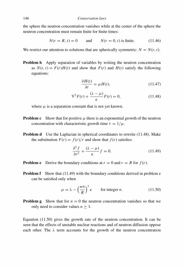
146 Conservation laws
the sphere the neutron concentration vanishes while at the center of the sphere theneutron concentration must remain finite for finite times:
N (r = R, t) = 0 and N (r = 0, t) is finite. (11.46)
We restrict our attention to solutions that are spherically symmetric: N = N (r, t).
Problem b Apply separation of variables by writing the neutron concentrationas N (r, t) = F(r )H (t) and show that F(r ) and H (t) satisfy the followingequations:
∂ H (t)
∂t= µH (t), (11.47)
∇2 F(r ) + (λ − µ)
κF(r ) = 0, (11.48)
where µ is a separation constant that is not yet known.
Problem c Show that for positive µ there is an exponential growth of the neutronconcentration with characteristic growth time τ = 1/µ.
Problem d Use the Laplacian in spherical coordinates to rewrite (11.48). Makethe substitution F(r ) = f (r )/r and show that f (r ) satisfies:
∂2 f
∂r2+ (λ − µ)
κf = 0. (11.49)
Problem e Derive the boundary conditions at r = 0 and r = R for f (r ).
Problem f Show that (11.49) with the boundary conditions derived in problem ecan be satisfied only when
µ = λ −(nπ
R
)2κ for integer n. (11.50)
Problem g Show that for n = 0 the neutron concentration vanishes so that weonly need to consider values n ≥ 1.
Equation (11.50) gives the growth rate of the neutron concentration. It can beseen that the effects of unstable nuclear reactions and of neutron diffusion opposeeach other. The λ term accounts for the growth of the neutron concentration

11.6 Viscosity and the Navier–Stokes equation 147
through fission reactions: this term makes the inverse growth rate µ morepositive. Conversely, the κ term accounts for diffusion: this term gives a negativecontribution to µ.
Problem h What value of n gives the largest growth rate? Show that exponentialgrowth of the neutron concentration (i.e. a nuclear explosion) can only occurwhen
R > π
√
κ
λ. (11.51)
This implies that a nuclear explosion can only occur when the ball of fissionablematerial is larger than a certain critical size. If the ball is smaller than the criticalsize, more neutrons diffuse out of it than are created by fission, hence the nuclearreaction stops. In some of the earliest nuclear devices an explosion was created bybringing two half spheres that each were stable together to form one whole spherethat was unstable.
Problem i Suppose you have a ball of fissionable material that is just unstableand that you shape this material into a cube rather than a ball. Do you expectthis cube to be stable or unstable? Do not use any equations!
11.6 Viscosity and the Navier–Stokes equation
Many fluids exhibit a certain degree of viscosity. In this section it will be shownthat viscosity can be seen as an ad-hoc description of the momentum current in afluid due to small-scale movements in the fluid. The starting point of the analysisis the equation of momentum conservation in a fluid:
∂(ρv)
∂t+ ∇ · (ρvv) = F (11.13)
In a real fluid, motion takes place at a large range of length scales from microscopiceddies to organized motions with a size comparable to the size of the fluid body.Whenever we describe a fluid, it is impossible to account for the motion at thevery small length scales. This is not only so in analytical descriptions, but it is inparticular the case in numerical simulations of fluid flow. For example, in currentweather prediction schemes the motion of the air is computed on a grid with adistance of about 100 km between the grid points. When you look at the weather itis obvious that there is considerable motion at smaller length scales (e.g. cumulusclouds indicating convection, fronts, etc.). In general one cannot simply ignore the

148 Conservation laws
motion at these short length scales because these small-scale fluid motions transportsignificant amounts of momentum, heat, and other quantities such as moisture [78].
One way to account for the effect of the small-scale motion is to express thesmall-scale motion in the large-scale motion. It is not obvious that this is consistentwith reality, but it appears to be the only way to avoid a complete description of thesmall-scale motion of the fluid (which would be impossible).
In order to do this, we assume that there is some length scale which separatesthe small-scale flow from the large-scale flow, and we decompose the velocity intoa long-wavelength component vL and a short-wavelength component vS:
v = vL + vS. (11.52)
In addition, we take spatial averages over a length scale that corresponds to thelength scale that distinguishes the large-scale flow from the small-scale flow. Thisaverage is indicated by angle brackets: 〈· · ·〉. The average of the small-scale flow iszero, 〈vS〉 = 0, while the average of the large-scale flow is equal to the large-scaleflow, 〈vL〉 = vL , because the large-scale flow by definition does not vary over theaveraging length. For simplicity we assume that the density does not vary.
Problem a Use the expressions (11.13) and (11.52) to show that the momentumequation for the large-scale flow is given by:
∂(ρvL)
∂t+ ∇ · (ρvLvL ) + ∇ · (〈ρvSvS〉) = F. (11.53)
Show in particular why this expression contains a contribution that is quadraticin the small-scale flow, but that the terms that are linear in vS do not contribute.
All the terms in (11.53) are familiar, except the last term on the left-hand side. Thisterm exemplifies the effect of the small-scale flow on the large-scale flow since itaccounts for the transport of momentum by the small-scale flow. It seems that atthis point further progress is impossible without knowing the small-scale flow vS .One way to make further progress is to express the small-scale momentum current〈ρvSvS〉 in the large-scale flow.
Consider the large-scale flow shown in Figure 11.3. Whatever the small-scalemotions are, in general they will have the character of mixing. In the example inthe figure, the momentum is large at the top of the figure and smaller at the bottom.As a first approximation one may assume that the small-scale motions transportmomentum in the direction opposite to the momentum gradient of the large-scaleflow. By analogy with (11.29) we can approximate the momentum transport by the
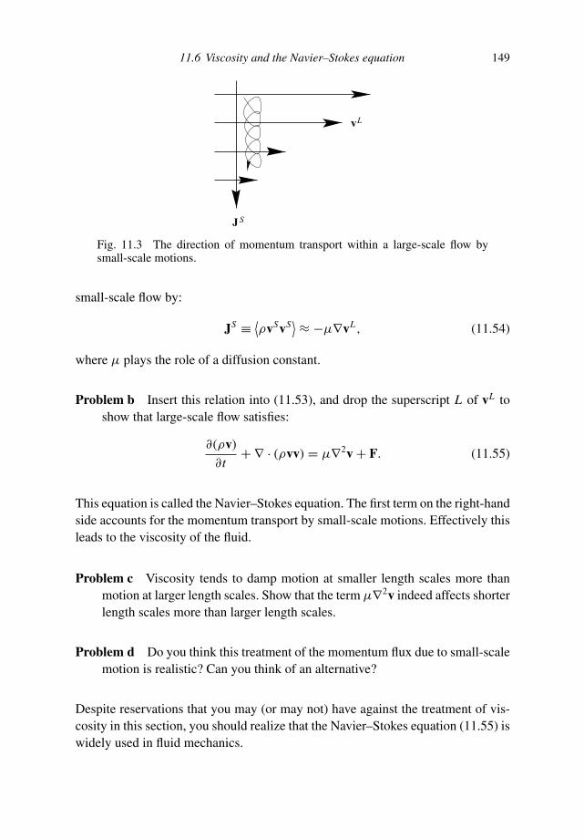
11.6 Viscosity and the Navier–Stokes equation 149
J S
vL
Fig. 11.3 The direction of momentum transport within a large-scale flow bysmall-scale motions.
small-scale flow by:
JS ≡ ⟨
ρvSvS⟩ ≈ −µ∇vL , (11.54)
where µ plays the role of a diffusion constant.
Problem b Insert this relation into (11.53), and drop the superscript L of vL toshow that large-scale flow satisfies:
∂(ρv)
∂t+ ∇ · (ρvv) = µ∇2v + F. (11.55)
This equation is called the Navier–Stokes equation. The first term on the right-handside accounts for the momentum transport by small-scale motions. Effectively thisleads to the viscosity of the fluid.
Problem c Viscosity tends to damp motion at smaller length scales more thanmotion at larger length scales. Show that the term µ∇2v indeed affects shorterlength scales more than larger length scales.
Problem d Do you think this treatment of the momentum flux due to small-scalemotion is realistic? Can you think of an alternative?
Despite reservations that you may (or may not) have against the treatment of vis-cosity in this section, you should realize that the Navier–Stokes equation (11.55) iswidely used in fluid mechanics.

150 Conservation laws
11.7 Quantum mechanics and hydrodynamics
As we saw in Section 8.4, the behavior of atomic particles is described bySchrodinger’s equation:
ih∂ψ(r, t)
∂t= − h2
2m∇2ψ(r, t) + V (r)ψ(r, t), (8.14)
rather than Newton’s law. In this section we reformulate the linear wave equation(8.14) as the laws of conservation of mass and momentum for a normal fluid. Inorder to do this we write the wavefunction ψ as
ψ = √ρ × e(i/h)ϕ. (11.56)
This equation is simply the decomposition of a complex function into its absolutevalue and its phase, hence ρ and ϕ are real functions. The factor h is a constantadded here for notational convenience. This constant is characteristic of quantummechanics and is called Planck’s constant.
Problem a Insert the decomposition (11.56) into Schrodinger’s equation (8.14),divide by
√ρe(i/h)ϕ and separate the result into real and imaginary parts to
show that ρ and ϕ satisfy the following differential equations:
∂ρ
∂t+ ∇ ·
(
ρ1
m∇ϕ
)
= 0, (11.57)
∂ϕ
∂t+ 1
2m|∇ϕ|2 + h2
8m
(
1
ρ2|∇ρ|2 − 2
ρ∇2ρ
)
= −V . (11.58)
The problem is that at this point we do not yet have a velocity. Let us define thefollowing velocity vector:
v ≡ 1
m∇ϕ. (11.59)
Problem b Show that this definition of the velocity is identical to the velocityobtained in (8.21) for a plane wave.
Problem c Show that with this definition of the velocity, (11.57) is identical tothe continuity equation:
∂ρ
∂t+ ∇ · (ρv) = 0. (11.6)

11.7 Quantum mechanics and hydrodynamics 151
Problem d In order to reformulate (11.58) as an equation of conservation ofmomentum, differentiate (11.58) with respect to xi . Then use the definition(11.59) and the relation between force and potential (F = − ∇V ) to write theresult as:
∂vi
∂t+ 1
2
∑
j
∂i (v jv j ) + h2
8m
[
∂i
(
1
ρ2|∇ρ|2
)
− 2∂i
(
1
ρ∇2ρ
)]
= 1
mFi .
(11.60)
The second term on the left-hand side does not look very much like the term∑
j ∂ j (ρv jvi ) in the left-hand side of (11.13). To make progress we need to rewritethe term
∑
j ∂i (v jv j ) as a term of the form∑
j ∂ j (v jvi ). In general these terms aredifferent.
Problem e Show that for the special case that the velocity is the gradient of ascalar function (as in expression (11.59)):
∑
j
1
2∂i (v jv j ) =
∑
j
∂ j (v jvi ). (11.61)
With this step we can rewrite the second term on the left-hand side of (11.60). Partof the third term in (11.60) we will designate as Qi :
Qi ≡ −1
8
[
∂i
(
1
ρ2|∇ρ|2
)
− 2∂i
(
1
ρ∇2ρ
)]
. (11.62)
Problem f Use (11.6) and (11.60)–(11.62) to derive that:
∂ (ρv)
∂t+ ∇ · (ρvv) = ρ
m
(
F + h2Q)
. (11.63)
Note that this equation is identical to the momentum equation (11.13). Thisimplies that the Schrodinger equation is equivalent to the continuity equation (11.6)and to the momentum equation (11.13) for a classical fluid. In Section 8.4 we sawthat atomic particles behave as waves rather than as point-like particles. In thissection we have discovered that these particles also behave like a fluid! This hasled to hydrodynamic formulations of quantum mechanics [48, 66]. In general,quantum-mechanical phenomena depend critically on Planck’s constant. Quantummechanics reduces to classical mechanics in the limit h → 0. The only place wherePlanck’s constant occurs in (11.63) is in the additional force: Q multiplied by the

152 Conservation laws
square of Planck’s constant. This implies that the action of the force term Q isfundamentally quantum-mechanical; it has no analogue in classical mechanics.
Problem g Suppose we consider a particle in one dimension that is representedby the following wave function:
ψ(x, t) = e−x2/L2ei(kx−ωt). (11.64)
Sketch the corresponding probability-density ρ and use (11.62) to deduce thatthe quantum force Q acts to broaden the wavefunction with time.
This example shows that (at least for this case) the quantum force Q makes the wave-function “spread out” with time. This reflects the fact that if a particle propagateswith time, its position becomes more and more uncertain.
The acoustic wave equation (8.7) cannot be transformed into the continuityequation (11.6) and the momentum equation (11.13), despite the fact that theseequations describe the conservation of mass and momentum in an acoustic medium.The reason for this paradox is that in the derivation of the acoustic wave equationfrom the continuity equation and the momentum equation, the advective terms∇ · (ρv) and ∇ · (ρvv) have been ignored. Once these terms have been ignoredthere is no transformation of variables that can bring them back. This contrasts theacoustic wave equation from the Schrodinger equation, which implicitly retains thephysics of the advection of mass and momentum.
12
Scale analysis
In most situations, the equations that we would like to solve in mathematical physicsare too complicated to solve analytically. One of the reasons for this is often thatan equation contains many different terms which make the problem simply toocomplex to be manageable. However, many of these terms may in practice be verysmall. Ignoring these small terms can simplify the problem to such an extent thatit can be solved in closed form. Moreover, by deleting terms that are small one isable to focus on the terms that are significant and that contain the relevant physics.In this sense, ignoring small terms can actually give a better physical insight intothe processes that really do matter.
Scale analysis is a technique in which one estimates the different terms in anequation by considering the scale over which the relevant parameters vary. This isan extremely powerful tool for simplifying problems. A comprehensive overviewof this technique with many applications is given by Kline [56] and in Chapter 6of Lin et al. [63]. Interesting examples of the application of scaling arguments tobiology are given by Vogel [113].
With the application of scale analysis one caveat must be made. One of themajor surprises of classical physics of the twentieth century was the discoveryof chaos in dynamical systems [104]. In a chaotic system small changes in theinitial conditions lead to a change in the time evolution of the system that growsexponentially with time. Deleting small terms from the equation of motion ofsuch a system can have a similar effect; the effects of omitting small terms canlead to changes in the system that may grow exponentially with time. This meansthat for chaotic systems one must be careful in omitting small terms from theequations.
The principle of scale analysis is first applied to the problem of determining thesense of rotation of a vortex in an emptying bathtub. Many of the equations thatare used in physics are differential equations. For this reason it is crucial in scaleanalysis to be able to estimate the order of magnitude of derivatives. The estimation
153

154 Scale analysis
of derivatives is therefore treated in Section 12.2. In subsequent sections this is thenapplied to a variety of different problems.
12.1 Vortex in a bathtub
Often when you empty a bathtub you can observe a beautiful vortex above the drainin the bathtub. When you ask people about the sense of rotation of this vortex manypeople will reply that the sense of rotation is in the counterclockwise direction onthe northern hemisphere and in the clockwise direction in the southern hemisphere(or vice versa). This statement is wrong and the easiest way to verify this is to take abath, empty the bathtub and observe that it is as easy to obtain a vortex that rotates inthe clockwise direction as it is to create a vortex that rotates in the counterclockwisedirection. In fact, if you have ever had the opportunity to take a bath in Nairobi,you would have had the chance to observe that on the equator (where the effectiverotation of the Earth vanishes) a bathtub drains in exactly the same way as at higherlatitudes.
Yet when you ask your friends you may find that it is very difficult to convincethem of these facts. In that case you may be able to convince them with a calculation.One approach would be to take the equations of fluid flow on a rotating Earth andcompute numerically in all details the flow in your bathtub. However, this approachis not only terribly impractical but it is also very difficult to carry out because youknow neither the detailed shape of your bathtub nor the initial conditions of thewater in the bathtub before you drain it. An even more serious drawback of thisapproach is that this numerical simulation does not give much physical insight. Atbest it gives a perfect simulation of the real bathtub, but in that case it would bebetter to do the experiment in the real bathtub.
As an alternative we can estimate the relative strength of the forces that are actingon the fluid in the vortex. In Figure 12.1 the forces are shown that act on a fluid parcelin a vortex on the Earth that rotates with angular velocity Ω. The dominant forcesare the pressure force Fpres that is associated with the pressure gradient in the fluid,the Coriolis force FCor due to the rotation of the Earth, and the centrifugal force Fcent
that is due to the circular motion of the fluid in the vortex. The rotational velocity ofthe vortex is denoted by ω. The only force that depends on the position on the Earthis the Coriolis force FCor. In Figure 12.1 this force points to the right-hand side of thevelocity vector; this is the case in the northern hemisphere whereas in the southernhemisphere this force would point to the left-hand side of the velocity vector. Thecentrifugal force always points outward from the vortex while the pressure forcealways points into the vortex. This means that any asymmetry between the behaviorof a vortex in the northern hemisphere and one in the southern hemisphere must bedue to the Coriolis force.
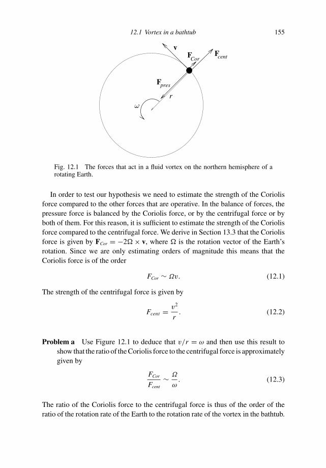
12.1 Vortex in a bathtub 155
presF
FcentFCor
v
r
Fig. 12.1 The forces that act in a fluid vortex on the northern hemisphere of arotating Earth.
In order to test our hypothesis we need to estimate the strength of the Coriolisforce compared to the other forces that are operative. In the balance of forces, thepressure force is balanced by the Coriolis force, or by the centrifugal force or byboth of them. For this reason, it is sufficient to estimate the strength of the Coriolisforce compared to the centrifugal force. We derive in Section 13.3 that the Coriolisforce is given by FCor = −2 × v, where is the rotation vector of the Earth’srotation. Since we are only estimating orders of magnitude this means that theCoriolis force is of the order
FCor ∼ Ωv. (12.1)
The strength of the centrifugal force is given by
Fcent = v2
r. (12.2)
Problem a Use Figure 12.1 to deduce that v/r = ω and then use this result toshow that the ratio of the Coriolis force to the centrifugal force is approximatelygiven by
FCor
Fcent∼ Ω
ω. (12.3)
The ratio of the Coriolis force to the centrifugal force is thus of the order of theratio of the rotation rate of the Earth to the rotation rate of the vortex in the bathtub.

156 Scale analysis
Problem b Assuming that the vortex rotates once a second, use the previousexpression to show that
FCor
Fcent∼ 10−5. (12.4)
This means that the Coriolis force is much smaller than all other forces thatare operating on the fluid parcel. The asymmetry in the balance of forces createdby the Coriolis force is in practice also much smaller than the asymmetry in theshape of the bathtub and the asymmetry in the initial conditions of the fluid motionbefore you drain the bathtub. We can conclude from this that the Earth’s rotationis negligible in the dynamics of the vortex; hence the sense of rotation of a vor-tex in a bathtub does not depend on the geographic location of the bathtub. Thisexample shows that one can sometimes learn more from simple physical argu-ments and estimates of orders of magnitude than from very complex numericalcalculations.
It follows from (12.3) that the centrifugal force and the Coriolis force are of thesame order of magnitude when the rotation rate of the fluid in the bathtub is of thesame order of magnitude as the Earth’s rotation.
Problem c Estimate the ratio of the Coriolis force to the centrifugal force for theatmospheric motion around a depression.
You will have found that for the atmosphere the Coriolis force is one of the domi-nant forces. This is the reason that in the northern hemisphere the air moves in thecounterclockwise direction around a low-pressure area and in the clockwise direc-tion around a high-pressure center (and vice versa on the southern hemisphere). Alow-pressure area is indeed very similar to the vortex in a bathtub. This analogy isin fact the cause of the misconception that the vortex in a bathtub always turns inone direction depending on geographic location. The major difference is, however,that the relative strengths of the forces that are operative in the atmosphere and ina bathtub are completely different. This result has been derived here with a simplescale analysis.
12.2 Three ways to estimate a derivative
In this section three different ways to estimate the derivative of a function f (x)are derived. The first way to estimate the derivative is to realize that the derivativeis nothing but the slope of the function f (x). Consider Figure 12.2 in which thefunction f (x) is assumed to be known at neighboring points x and x + h.

12.2 Three ways to estimate a derivative 157
x x + h
f (x)
f(x + h)
Fig. 12.2 The slope of a function f (x) that is known at positions x and x + h.
Problem a Deduce from the geometry of this figure that the slope of the functionat x is approximately given by [ f (x + h) − f (x)]/h.
Since the slope is the derivative this means that the derivative of the function isapproximately given by
d f
dx≈ f (x + h) − f (x)
h. (12.5)
The second way to derive the same result is to realize that the derivative is definedby the following limit:
d f
dx≡ lim
h→0
f (x + h) − f (x)
h. (12.6)
If we consider the right-hand side of this expression without taking the limit, wedo not quite obtain the derivative, but as long as h is sufficiently small we obtainthe approximation (12.5).
The problem with estimating the derivative of f (x) in the previous ways is thatalthough we obtain an estimate of the derivative, we do not know how good theseestimates are. We know that if f (x) was a straight line, which has a constant slope,the estimate (12.5) would be exact. Hence it is the deviation of f (x) from a straightline that makes (12.5) only an approximation. This means that it is the curvatureof f (x) that accounts for the error in the approximation (12.5). The third way ofestimating the derivative provides this error estimate as well.
Problem b Consider the Taylor series (3.17). Truncate this series after the secondorder term and solve the resulting expression for d f/dx to derive that
d f
dx= f (x + h) − f (x)
h− 1
2
d2 f
dx2h + · · · , (12.7)
where the dots indicate terms of order h2 and higher.

158 Scale analysis
In the limit h → 0 the last term vanishes and (12.6) is obtained. When one ig-nores the last term in (12.7) for finite h one once again obtains the approximation(12.5).
Problem c Use (12.7) to show that the error made in the approximation (12.5)indeed depends on the curvature of the function f (x).
The approximation (12.5) has a variety of applications. The first is the numericalsolution of differential equations. Suppose one has a differential equation that cannotbe solved in closed form. To fix our minds, consider the differential equation
d f
dx= G( f (x), x), (12.8)
with initial value
f (0) = f0. (12.9)
If this equation cannot be solved in closed form, one can solve it numerically byevaluating the function f (x) not for every value of x , but only at a finite number ofx-values that are separated by a distance h. These points xn are given by xn = nh,and the function f (x) at location xn is denoted by fn:
fn ≡ f (xn). (12.10)
Problem d Show that the derivative d f/dx at location xn can be approximatedby:
d f
dx(xn) = 1
h( fn+1 − fn). (12.11)
Problem e Insert this result into the differential equation (12.8) and solve theresulting expression for fn+1 to show that:
fn+1 = fn + hG( fn, xn). (12.12)
This is all we need to numerically solve the differential equation (12.8) with theboundary condition (12.9). Once fn is known, (12.12) can be used to computefn+1. This means that the function can be computed at all values of the grid pointsxn recursively. To start this process, one uses the boundary condition (12.9) thatgives the value of the function at location x0 = 0. This technique for estimatingthe derivative of a function can be extended to higher order derivatives as well sothat second order differential equations can also be solved numerically. In prac-tice, one has to pay serious attention to the stability of the numerical solution.
12.3 Advective terms in the equation of motion 159
The requirements of stability and numerical efficiency have led to many refine-ments of the numerical methods for solving differential equations. The interestedreader can consult Press et al. [84] for an introduction and many practical algo-rithms.
The estimate (12.5) has a second important application because it allows us toestimate the order of magnitude of a derivative. Suppose a function f (x) variesover a characteristic range of values F and that this variation takes place over acharacteristic distance L . It follows from (12.5) that the derivative of f (x) is of theorder of the ratio of the variation of the function f (x) divided by the length scaleover which the function varies. In other words:
∣
∣
∣
∣
d f
dx
∣
∣
∣
∣
≈ variation of the function f (x)
length scale of the variation∼ F
L. (12.13)
In this expression the term ∼ F/L indicates that the derivative is of the order F/L .Note that this is not in general an accurate estimate of the precise value of thefunction f (x), it only provides us with an estimate of the order of magnitude of aderivative. However, this is all we need to carry out scale analysis.
Problem f Suppose f (x) is a sinusoidal wave with amplitude A andwavelength λ:
f (x) = A sin
(
2πx
λ
)
. (12.14)
Show that (12.13) implies that the order of magnitude of the derivative of thisfunction is given by |d f/dx | ∼ O (A/λ). Compare this estimate of the orderof magnitude with the true value of the derivative and pay attention both tothe numerical value as well as to the spatial variation.
From the previous estimate we can learn two things. First, the estimate (12.13) isonly a rough estimate that locally can be very poor. One should always be awarethat (12.13) may break down at certain points and that this can cause errors inthe subsequent scale analysis. Second, (12.13) differs by a factor 2π from the truederivative. However, 2π ≈ 6.28, which is not a small number (compared to 1).Therefore you must be aware that hidden numerical factors may enter scalingarguments.
12.3 Advective terms in the equation of motion
As a first example of scale analysis we consider the role of advective terms in theequation of motion. As shown in (11.12) the equation of motion for a continuous
160 Scale analysis
medium is given by
∂v∂t
+ v · ∇v = 1
ρF. (12.15)
Note that we have divided by the density compared to the original expression(11.12). This equation can describe the propagation of acoustic waves when F isthe pressure force, and it accounts for elastic waves when F is given by the elasticforces in the medium. We consider the situation in which waves with a wavelengthλ and a period T propagate through the medium.
The advective terms v · ∇v often pose a problem in solving this equation. This isbecause the partial time-derivative ∂v/∂t is linear in the velocity v but the advectiveterms v · ∇v are nonlinear in the velocity v. Since linear equations are in generalmuch easier to solve than nonlinear equations it is useful to know under whichconditions the advective terms v · ∇v can be ignored compared with the partialderivative ∂v/∂t .
Problem a Let the velocity of the continuous medium have a characteristic valueV . Show that |∂v/∂t | ∼ V/T and that |v · ∇v| ∼V 2/λ.
Problem b Show that this means that the ratio of the advective terms to the partialtime-derivative is given by
|v · ∇v||∂v/∂t | ∼ V
c, (12.16)
where c = λ/T is the phase velocity with which the waves propagate throughthe medium.
This result implies that the advective terms can be ignored when the velocity ofthe medium itself is much less than the velocity of the waves propagating throughthe medium:
V c. (12.17)
In other words, when the amplitude of the wave motion is so small that the velocityof the particle motion in the medium is much less than the phase velocity of thewaves, one can ignore the advective terms in the equation of motion.
Problem c Suppose an earthquake causes a ground displacement of 1 mm at afrequency of 1 Hz at a large distance. The wave velocity of seismic P-wavesis of the order of 5 km/s near the surface. Show that in that case V/c ∼ 10−6.
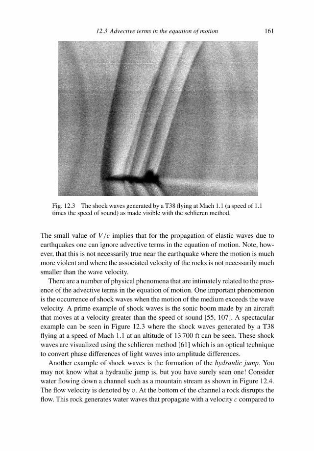
12.3 Advective terms in the equation of motion 161
Fig. 12.3 The shock waves generated by a T38 flying at Mach 1.1 (a speed of 1.1times the speed of sound) as made visible with the schlieren method.
The small value of V/c implies that for the propagation of elastic waves due toearthquakes one can ignore advective terms in the equation of motion. Note, how-ever, that this is not necessarily true near the earthquake where the motion is muchmore violent and where the associated velocity of the rocks is not necessarily muchsmaller than the wave velocity.
There are a number of physical phenomena that are intimately related to the pres-ence of the advective terms in the equation of motion. One important phenomenonis the occurrence of shock waves when the motion of the medium exceeds the wavevelocity. A prime example of shock waves is the sonic boom made by an aircraftthat moves at a velocity greater than the speed of sound [55, 107]. A spectacularexample can be seen in Figure 12.3 where the shock waves generated by a T38flying at a speed of Mach 1.1 at an altitude of 13 700 ft can be seen. These shockwaves are visualized using the schlieren method [61] which is an optical techniqueto convert phase differences of light waves into amplitude differences.
Another example of shock waves is the formation of the hydraulic jump. Youmay not know what a hydraulic jump is, but you have surely seen one! Considerwater flowing down a channel such as a mountain stream as shown in Figure 12.4.The flow velocity is denoted by v. At the bottom of the channel a rock disrupts theflow. This rock generates water waves that propagate with a velocity c compared to
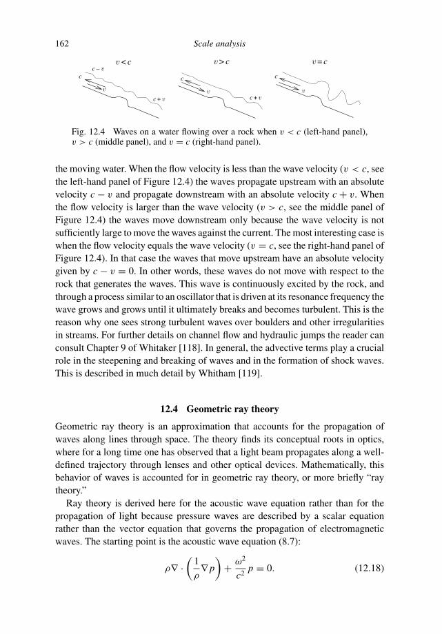
162 Scale analysis
c c c
Fig. 12.4 Waves on a water flowing over a rock when v < c (left-hand panel),v > c (middle panel), and v = c (right-hand panel).
the moving water. When the flow velocity is less than the wave velocity (v < c, seethe left-hand panel of Figure 12.4) the waves propagate upstream with an absolutevelocity c − v and propagate downstream with an absolute velocity c + v. Whenthe flow velocity is larger than the wave velocity (v > c, see the middle panel ofFigure 12.4) the waves move downstream only because the wave velocity is notsufficiently large to move the waves against the current. The most interesting case iswhen the flow velocity equals the wave velocity (v = c, see the right-hand panel ofFigure 12.4). In that case the waves that move upstream have an absolute velocitygiven by c − v = 0. In other words, these waves do not move with respect to therock that generates the waves. This wave is continuously excited by the rock, andthrough a process similar to an oscillator that is driven at its resonance frequency thewave grows and grows until it ultimately breaks and becomes turbulent. This is thereason why one sees strong turbulent waves over boulders and other irregularitiesin streams. For further details on channel flow and hydraulic jumps the reader canconsult Chapter 9 of Whitaker [118]. In general, the advective terms play a crucialrole in the steepening and breaking of waves and in the formation of shock waves.This is described in much detail by Whitham [119].
12.4 Geometric ray theory
Geometric ray theory is an approximation that accounts for the propagation ofwaves along lines through space. The theory finds its conceptual roots in optics,where for a long time one has observed that a light beam propagates along a well-defined trajectory through lenses and other optical devices. Mathematically, thisbehavior of waves is accounted for in geometric ray theory, or more briefly “raytheory.”
Ray theory is derived here for the acoustic wave equation rather than for thepropagation of light because pressure waves are described by a scalar equationrather than the vector equation that governs the propagation of electromagneticwaves. The starting point is the acoustic wave equation (8.7):
ρ∇ ·(
1
ρ∇ p
)
+ ω2
c2p = 0. (12.18)

12.4 Geometric ray theory 163
For simplicity the source term on the right-hand side has been set to zero. In addition,the relation c2 = κ/ρ has been used to eliminate the bulk modulus κ in favor of thewave velocity c. Both the density ρ and the wave velocity are arbitrary functionsof space.
In general it is not possible to solve this differential equation in closed form.Instead we seek an approximation by writing the pressure as:
p(r, ω) = A(r, ω)eiψ(r,ω), (12.19)
with A and ψ real functions. Any function p(r, ω) can be written in this way.
Problem a Insert the solution (12.19) in the acoustic wave equation (12.18), sep-arate the real and imaginary parts of the resulting equation to deduce that(12.18) is equivalent to the following equations:
∇2 A︸︷︷︸
(1)
− A |∇ψ |2︸ ︷︷ ︸
(2)
− 1
ρ(∇ρ · ∇ A)
︸ ︷︷ ︸
(3)
+ ω2
c2A
︸︷︷︸
(4)
= 0, (12.20)
and
2 (∇ A · ∇ψ) + A∇2ψ − 1
ρ(∇ρ · ∇ψ) A = 0. (12.21)
These equations are even harder to solve than the acoustic wave equation be-cause they are nonlinear in the unknown functions A and ψ whereas the acousticwave equation is linear in the pressure p. However, (12.20) and (12.21) form agood starting point for making the ray-geometric approximation. First we analyze(12.20).
Assume that the density varies on a length scale Lρ , and that the amplitudeA of the wave field varies on a characteristic length scale L A. Furthermore thewavelength of the waves is denoted by λ.
Problem b Explain that the wavelength is the length scale over which the phaseψ of the waves varies.
Problem c Use the results of Section 12.2 to obtain the following estimates ofthe order of magnitude of the terms (1)–(4) in equation (12.20):
∣
∣∇2 A∣
∣ ∼ A
L2A
, A |∇ψ |2 ∼ A
λ2 ,
∣
∣
∣
∣
1
ρ(∇ρ · ∇ A)
∣
∣
∣
∣
∼ A
L A Lρ
,ω2
c2A ∼ A
λ2 .
⎫
⎪
⎪
⎬
⎪
⎪
⎭
(12.22)

164 Scale analysis
To make further progress we assume that the length scales of both the densityvariations and the amplitude variations are much longer than a wavelength: λ L A
and λ Lρ .
Problem d Show that under this assumption terms (1) and (3) in equation (12.20)are much smaller than terms (2) and (4).
Problem e Convince yourself that ignoring terms (1) and (3) in (12.20) gives thefollowing (approximate) expression:
|∇ψ |2 = ω2
c2. (12.23)
Problem f The approximation (12.23) was obtained under the premise that|∇ψ | ∼ 1/λ. Show that this assumption is satisfied by the function ψ in(12.23).
Whenever one makes approximations by deleting terms that scale analysis predictsto be small, one has to check that the final solution is consistent with the scaleanalysis that is used to derive the approximation.
Note that the original equation (12.20) contains both the amplitude A and thephase ψ but that (12.23) contains the phase only. The approximation that we havemade has thus decoupled the phase from the amplitude; this simplifies the problemconsiderably. The frequency enters the right-hand side of this equation only througha simple multiplication with ω2. The frequency dependence of ψ can be found bysubstituting
ψ(r, ω) = ωτ (r). (12.24)
Problem g Show that after this substitution (12.23) and (12.21) are given by
|∇τ (r)|2 = 1
c2, (12.25)
and
2 (∇ A · ∇τ ) + A∇2τ − 1
ρ(∇ρ · ∇τ ) A = 0. (12.26)
According to (12.25) the function τ (r) does not depend on frequency. Notethat (12.26) for the amplitude does not contain any frequency dependence either.This means that the amplitude also does not depend on frequency: A = A(r). Thishas important consequences for the shape of the wave field in the ray-geometric
12.4 Geometric ray theory 165
approximation. Suppose that the wave field is excited by a source function s(t) inthe time domain that is represented in the frequency domain by a complex functionS(ω). (The forward and backward Fourier transform is defined by (15.42) and(15.43).) In the frequency domain the response is given by (12.19) multiplied withthe source function S(ω). Using that A and τ do not depend on frequency, thepressure in the time domain can be written as:
p(r, t) =∫ ∞
−∞A(r)eiωτ (r)e−iωt S(ω) dω. (12.27)
Problem h Use this expression to show that the pressure in the time domain canbe written as:
p(r, t) = A(r)s(t − τ (r)). (12.28)
This is an important result because it implies that the time dependence of the wavefield is everywhere given by the same source-time function s(t). In a ray-geometricapproximation the shape of the waveforms is everywhere the same. There are nofrequency-dependent effects in a ray-geometric approximation.
Problem i Explain why this implies that geometric ray theory cannot be used toexplain why the sky is blue.
The absence of any frequency-dependent wave propagation effects is both thestrength and the weakness of ray theory. It is a strength because the wave fields canbe computed in a simple way once τ (r) and A(r) are known. The theory also tellsus that this is an adequate description of the wave field as long as the frequency issufficiently high that λ L A and λ Lρ . However, many wave propagation phe-nomena are in practice frequency-dependent, and it is the weakness of ray theorythat it cannot account for these phenomena.
According to (12.28) the function τ (r) accounts for the time delay of the wavesto travel to the point r. Therefore, τ (r) is the travel time of the wave field. Thetravel time is described by the differential equation (12.25); this equation is calledthe eikonal equation.
Problem j Show that it follows from the eikonal equation that ∇τ can be writtenas:
∇τ = n/c, (12.29)
where n is a unit vector. Show also that n is perpendicular to the surfaceτ = const .

166 Scale analysis
The vector n defines the direction of the rays along which the wave energy prop-agates through the medium. Taking suitable derivatives of (12.29) one can derivethe equation of kinematic ray-tracing. This is a second order differential equa-tion for the position of the rays; details are given by Virieux [112] or Aki andRichards [3].
Once τ (r) is known, one can compute the amplitude A(r) from (12.26). We havenot yet applied any scale analysis to this expression. We will not do so, because itcan be solved exactly. Let us first simplify this differential equation by consideringthe dependence on the density ρ in more detail.
Problem k Write A = ρα B, where the constant α is not yet determined. Showthat the transport equation results in the following differential equation forB(r):
(2α − 1) (∇ρ · ∇τ ) B + 2ρ (∇ B · ∇τ ) + ρB∇2τ = 0. (12.30)
Choose the constant α in such a way that the gradient of the density disap-pears from the equation and show that the remaining terms can be written as∇ · (
B2∇τ) = 0. Finally show using (12.29) that this implies the following
differential equation for the amplitude:
∇ ·(
1
ρcA2n
)
= 0. (12.31)
Equation (12.31) states that the divergence of the vector(
A2/ρc)
n vanishes,hence the flux of this vector through any closed surface that does not containthe source of the wave-field vanishes, see Section 8.1. This is not surprising, be-cause the vector
(
A2/ρc)
n accounts for the energy flux of acoustic waves. Ex-pression (12.31) implies that the net flux of this vector through any closed sur-face is equal to zero. This means that all the energy that flows into the surfacemust also flow out through the surface again. The transport equation in the form(12.31) is therefore a statement of energy conservation. Virieux [112] or Aki andRichards [3] show how one can compute this amplitude once the location of therays is known.
An interesting complication arises when the energy is focused at a point or on asurface in space. Such an area of focusing is called a caustic. A familiar exampleof a caustic is the rainbow. One can show that at a caustic, the ray-geometricapproximation leads to an infinite amplitude of the wave field [112].
Problem l Show that when the amplitude becomes infinite in a finite region ofspace the condition λ L A must be violated.
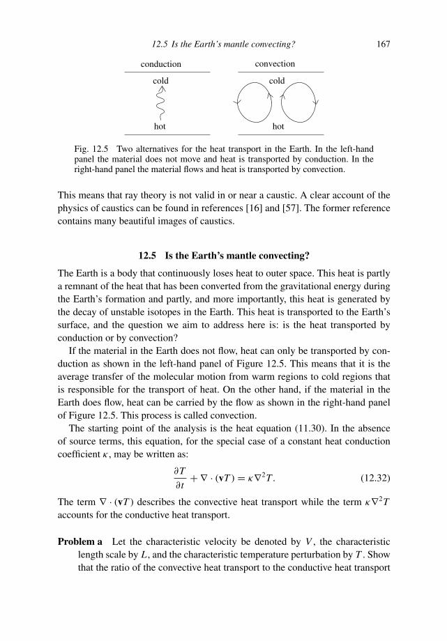
12.5 Is the Earth’s mantle convecting? 167
hot
cold cold
hot
conduction convection
Fig. 12.5 Two alternatives for the heat transport in the Earth. In the left-handpanel the material does not move and heat is transported by conduction. In theright-hand panel the material flows and heat is transported by convection.
This means that ray theory is not valid in or near a caustic. A clear account of thephysics of caustics can be found in references [16] and [57]. The former referencecontains many beautiful images of caustics.
12.5 Is the Earth’s mantle convecting?
The Earth is a body that continuously loses heat to outer space. This heat is partlya remnant of the heat that has been converted from the gravitational energy duringthe Earth’s formation and partly, and more importantly, this heat is generated bythe decay of unstable isotopes in the Earth. This heat is transported to the Earth’ssurface, and the question we aim to address here is: is the heat transported byconduction or by convection?
If the material in the Earth does not flow, heat can only be transported by con-duction as shown in the left-hand panel of Figure 12.5. This means that it is theaverage transfer of the molecular motion from warm regions to cold regions thatis responsible for the transport of heat. On the other hand, if the material in theEarth does flow, heat can be carried by the flow as shown in the right-hand panelof Figure 12.5. This process is called convection.
The starting point of the analysis is the heat equation (11.30). In the absenceof source terms, this equation, for the special case of a constant heat conductioncoefficient κ , may be written as:
∂T
∂t+ ∇ · (vT ) = κ∇2T . (12.32)
The term ∇ · (vT ) describes the convective heat transport while the term κ∇2Taccounts for the conductive heat transport.
Problem a Let the characteristic velocity be denoted by V , the characteristiclength scale by L , and the characteristic temperature perturbation by T . Showthat the ratio of the convective heat transport to the conductive heat transport
168 Scale analysis
is of the following order:
convective heat transport
conductive heat transport∼ V L
κ. (12.33)
This estimate gives the ratio of the two modes of heat transport, but it doesnot help us much yet because we do not know the order of magnitude V of theflow velocity. This quantity can be obtained from the Navier–Stokes equation ofSection 11.6:
∂(ρv)
∂t+ ∇ · (ρvv) = µ∇2v + F. (11.55)
The force F on the right-hand side is the buoyancy force that is associated withthe flow, while the term µ∇2v accounts for the viscosity of the flow with viscositycoefficient µ. The mantle of the Earth is extremely viscous and mantle convection(if it exists at all) is a slow process. We therefore assume that the inertia term∂(ρv)/∂t and the advection term ∇ · (ρvv) are small compared to the viscous termµ∇2v. (This assumption would have to be supported by a proper scale analysis.)Under this assumption, the mantle flow is predominantly governed by a balancebetween the viscous force and the buoyancy force:
µ∇2v = −F. (12.34)
The next step is to relate the buoyancy to the temperature perturbation T . Atemperature perturbation T from a reference temperature T0 leads to a densityperturbation ρ from the reference density ρ0 given by:
ρ = −αT . (12.35)
In this expression α is the thermal expansion coefficient which accounts for theexpansion or contraction of material due to temperature changes.
Problem b Explain why for most materials α > 0. A notable exception is waterat temperatures below 4 C.
Problem c Write ρ (T0 + T ) = ρ0 + ρ and use the Taylor expansion (3.11) trun-cated after the first order term to show that the expansion coefficient is givenby α = −∂ρ/∂T .
Problem d The buoyancy force is given by Archimedes’s law which states thatthis force equals the weight of the displaced fluid. Use this result, (12.34), and
12.6 Making an equation dimensionless 169
(12.35) in a scale analysis to show that the velocity is of the following order:
V ∼ gαTL2
µ, (12.36)
where g is the acceleration of gravity.
Problem e Use this to derive that the ratio of the convective heat transport to theconductive heat transport is given by
convective heat transport
conductive heat transport∼ gαTL3
µκ. (12.37)
The right-hand side of this expression is dimensionless, and is called the Rayleighnumber which is denoted by Ra:
Ra ≡ gαTL3
µκ. (12.38)
The Rayleigh number is an indicator for the mode of heat transport. When Ra 1, heat is predominantly transported by convection. When the thermal expansioncoefficient α is large and when the viscosity µ and the heat conduction coefficientκ are small the Rayleigh number is large and heat is transported by convection.
Problem f Explain physically why a large value of α and small values of µ andκ lead to convective heat transport rather than conductive heat transport.
Dimensionless numbers play a crucial role in fluid mechanics. A discussion of theRayleigh number and other dimensionless diagnostics such as the Prandtl numberand the Grashof number can be found in Section 14.2 of Tritton [108]. The implica-tions of the different values of the Rayleigh number on the character of convectionin the Earth’s mantle is discussed in references [77] and [110]. Of course, if onewants to use a scale analysis one must know the values of the physical propertiesinvolved. For the Earth’s mantle, the thermal expansion coefficient α is not verywell known because of the complications involved in laboratory measurements ofthe thermal expansion under the extremely high ambient pressure of the Earth’smantle [29].
12.6 Making an equation dimensionless
Usually the terms in equations that one wants to analyze have a physical dimensionsuch as temperature, velocity, etc. It can sometimes be useful to rescale all thevariables in the equation in such a way that the rescaled variables are dimensionless.

170 Scale analysis
This is convenient when setting up numerical solutions of the equations, and italso introduces dimensionless numbers that govern the physics of the problem ina natural way. As an example we will apply this technique to the heat equation(12.32).
Any variable can be made dimensionless by dividing out a constant that hasthe dimension of the variable. As an example, let the characteristic temperaturevariation be denoted by T0, then the dimensional temperature perturbation can bewritten as:
T = T0T′. (12.39)
The quantity T′
is dimensionless. Note that in this section T is the absolute tem-perature whereas in the previous section T denoted the temperature perturbation.
In this section, dimensionless variables are denoted by a prime. For example, letthe characteristic time used to scale the time variable be denoted by τ , then:
t = τ t′. (12.40)
We can still leave τ open and later choose a value that simplifies the equations asmuch as possible. Of course when we want to express the heat equation (12.32) inthe new time variable we need to specify how the dimensional time-derivative ∂/∂tis related to the dimensionless time-derivative ∂/∂t
′.
Problem a Use the chain rule for differentiation to show that
∂
∂t= 1
τ
∂
∂t ′ . (12.41)
Problem b Let the velocity be scaled with the characteristic velocity (12.36):
v = gαT0L2
µv
′, (12.42)
and let the position vector be scaled with the characteristic length L of thesystem: r = Lr
′. Use a result similar to (12.41) to convert the spatial derivatives
to the new space coordinate and rescale all terms in the heat equation (12.32)to derive the following dimensionless form of this equation
1
τ
∂T′
∂t ′︸ ︷︷ ︸
(1)
+ gαT0L
µ∇′ ·
(
v′T
′)
︸ ︷︷ ︸
(2)
= κ
L2∇′2T
︸ ︷︷ ︸
(3)
, (12.43)
where ∇′is the gradient operator with respect to the dimensionless coordi-
nates r′.
12.6 Making an equation dimensionless 171
At this point we have not yet specified the time scale τ for the scaling of thetime variable. There are three possible situations that determine τ . First, when term(2) is much larger than term (3), the time derivative (1) balances term (2). Second,when term (3) is much larger than term (2), the time derivative balances term (3).The third possibility is that terms (2) and (3) are of the same order of magnitude,in which case the balance of terms is more complex.
Problem c Show that the ratio of term (2) to term (3) is given by the Rayleighnumber which is defined in (12.38).
In this expression all the primed terms are (by definition) of order one. At thispoint we assume that the convective heat transport dominates the conductive heattransport, that is that Ra 1. This means that term (2) is much larger than term(3), hence the time derivative in term (1) must be of the same order as the convectiveterm (2). Terms (1) and (2) can therefore balance only when
1
τ= gαT0L
µ. (12.44)
This condition determines the time scale of the evolution of the convecting system.
Problem d Show that with this choice of τ the dimensionless heat equation isgiven by:
∂T′
∂t ′ + ∇′ ·(
v′T
′) = 1
Ra∇′2T
′, (12.45)
where Ra is the Rayleigh number.
The advantage of this dimensionless equation over the original heat equation is that(12.45) contains only a single constant Ra, whereas the dimensional heat equation(12.32) depends on a large number of constants. In addition, the scaling of theheat equation has led in a natural way to the key role of the Rayleigh number inthe mode of heat transport in a fluid. Since the Rayleigh number is assumed to belarge, 1/Ra 1 and the last term can be seen as a small perturbation. One caneither delete this term, or treat it with perturbation theory as described in Chapter23. The last term in (12.45) contains the highest spatial derivatives of that equationbecause it contains second order space derivatives whereas the other terms eitherhave no space derivatives (term (1)) or only first order space derivatives (term (2)).Deleting this term turns (12.45) from a second order differential equation (in thespace variables) into a first order differential equation. This entails a change in thenumber of boundary conditions that need to be imposed. As shown in Section 23.7
172 Scale analysis
the last term in (12.45) constitutes a singular perturbation, and one should becareful in deleting this (small) term altogether.
Transforming dimensional equations into dimensionless equations is often usedto derive the relevant dimensionless physical constants of the system as well asto set up algorithms for solving equations numerically. The basic rationale behindthis approach is that the physical units that are used are completely arbitrary. Itis immaterial whether we express length in meters or in inches, but of coursethe numerical value of a given length changes when we change from meters toinches. Making the system dimensionless removes all physical units from the systembecause all the resulting terms in the equation are dimensionless. This has thedrawback that dimensional analysis cannot be used to check for errors, as shownin Section 2.2.
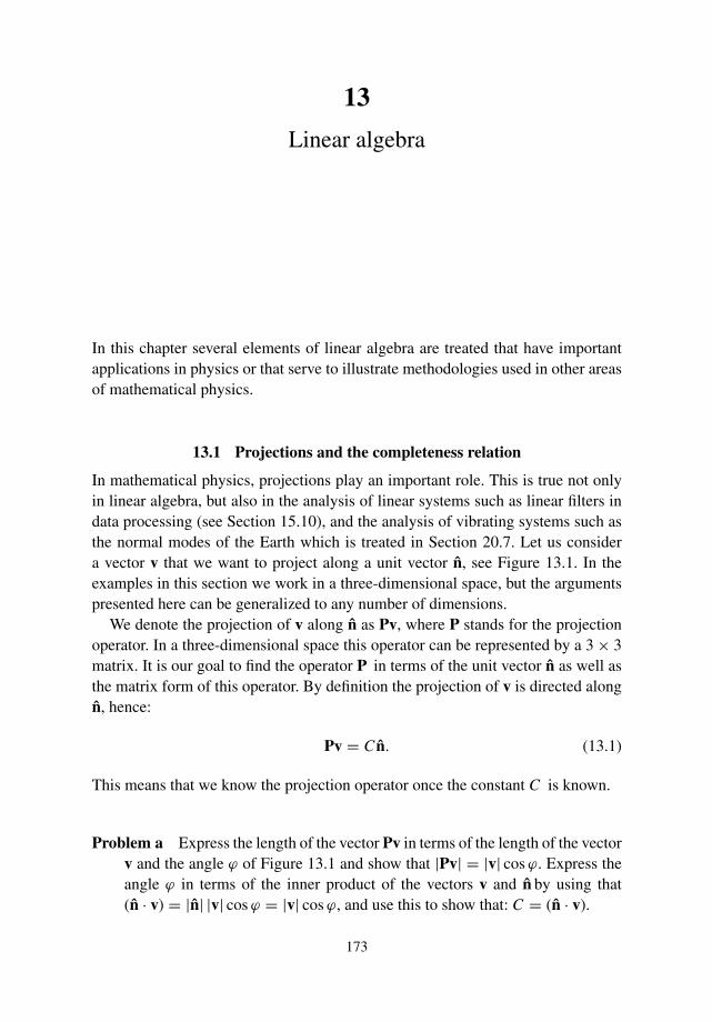
13
Linear algebra
In this chapter several elements of linear algebra are treated that have importantapplications in physics or that serve to illustrate methodologies used in other areasof mathematical physics.
13.1 Projections and the completeness relation
In mathematical physics, projections play an important role. This is true not onlyin linear algebra, but also in the analysis of linear systems such as linear filters indata processing (see Section 15.10), and the analysis of vibrating systems such asthe normal modes of the Earth which is treated in Section 20.7. Let us considera vector v that we want to project along a unit vector n, see Figure 13.1. In theexamples in this section we work in a three-dimensional space, but the argumentspresented here can be generalized to any number of dimensions.
We denote the projection of v along n as Pv, where P stands for the projectionoperator. In a three-dimensional space this operator can be represented by a 3 × 3matrix. It is our goal to find the operator P in terms of the unit vector n as well asthe matrix form of this operator. By definition the projection of v is directed alongn, hence:
Pv = C n. (13.1)
This means that we know the projection operator once the constant C is known.
Problem a Express the length of the vector Pv in terms of the length of the vectorv and the angle ϕ of Figure 13.1 and show that |Pv| = |v| cos ϕ. Express theangle ϕ in terms of the inner product of the vectors v and n by using that(n · v) = |n| |v| cos ϕ = |v| cos ϕ, and use this to show that: C = (n · v).
173
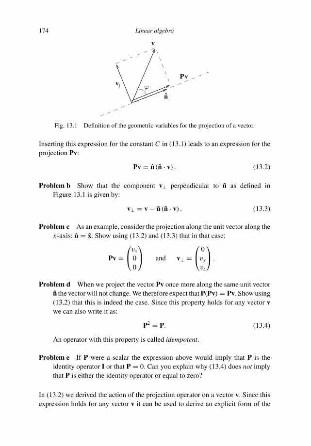
174 Linear algebra
vP
n
v
v
Fig. 13.1 Definition of the geometric variables for the projection of a vector.
Inserting this expression for the constant C in (13.1) leads to an expression for theprojection Pv:
Pv = n (n · v) . (13.2)
Problem b Show that the component v⊥ perpendicular to n as defined inFigure 13.1 is given by:
v⊥ = v − n (n · v) . (13.3)
Problem c As an example, consider the projection along the unit vector along thex-axis: n = x. Show using (13.2) and (13.3) that in that case:
Pv =⎛
⎝
vx
00
⎞
⎠ and v⊥ =⎛
⎝
0vy
vz
⎞
⎠ .
Problem d When we project the vector Pv once more along the same unit vectorn the vector will not change. We therefore expect that P(Pv) = Pv. Show using(13.2) that this is indeed the case. Since this property holds for any vector vwe can also write it as:
P2 = P. (13.4)
An operator with this property is called idempotent.
Problem e If P were a scalar the expression above would imply that P is theidentity operator I or that P = 0. Can you explain why (13.4) does not implythat P is either the identity operator or equal to zero?
In (13.2) we derived the action of the projection operator on a vector v. Since thisexpression holds for any vector v it can be used to derive an explicit form of the

13.1 Projections and the completeness relation 175
projection operator:
P = nnT . (13.5)
This expression should not be confused with the inner product (n · n); instead itdenotes the dyad of the vector n and itself. The superscript T denotes the transposeof a vector or matrix. The transpose of a vector (or matrix) is found by interchangingits rows and columns. For example, the transpose AT of a matrix A is defined by:
ATi j = A ji , (13.6)
and the transpose of the vector u is defined by:
uT = (ux , uy, uz) when u =⎛
⎝
ux
uy
uz
⎞
⎠ , (13.7)
that is taking the transpose converts a column vector into a row vector. The projectionoperator P is written in (13.5) as a dyad. In general the dyad T of two vectors u andv is defined as
T = uvT . (13.8)
This expression simply means that the components Ti j of the dyad are defined by
Ti j = uiv j , (13.9)
where ui is the i-component of u and v j is the j-component of v.In the literature you will find different notations for the inner product of two
vectors. The inner product of the vectors u and v is sometimes written as
(u · v) = uT v. (13.10)
Problem f Considering the vector v as a 3 × 1 matrix and the vector vT as a1 × 3 matrix, show that the notation used on the right-hand sides of (13.10)and (13.8) is consistent with the normal rules for matrix multiplication.
Equation (13.5) relates the projection operator P to the unit vector n. From thisthe representation of the projection operator as a 3 × 3 matrix can be found bycomputing the dyad nnT .
Problem g Show that the operator for the projection along the unit vector
n = 1√14
⎛
⎝
123
⎞
⎠
176 Linear algebra
is given by
P = 1
14
⎛
⎝
1 2 32 4 63 6 9
⎞
⎠ .
Verify explicitly that for this example Pn = n, and explain this result.
Up to this point we have projected the vector v along a single unit vector n.Suppose we have a set of mutually orthogonal unit vectors ni . The fact that theseunit vectors are mutually orthogonal means that the different unit vectors are per-pendicular to each other:
(
ni · n j) = 0 when i = j . We can project v on each of
these unit vectors and add these projections. This gives us the projection of v onthe subspace spanned by the unit vectors ni :
Pv =∑
i
ni (ni · v) . (13.11)
When the unit vectors ni span the full space we are working in, the projectedvector is identical to the original vector. To see this, consider for example a three-dimensional space. Any vector can be decomposed into its components along thex-, y-, and z-axes, and this can be written as:
v = vx x + vy y + vz z = x (x · v) + y (y · v) + z (z · v) ; (13.12)
note that this expression has the same form as (13.11). This implies that when in(13.11) we sum over a set of unit vectors that completely spans the space we areworking in, the right-hand side of (13.11) is identical to the original vector v, thatis
∑
i ni (ni · v) = v. The operator of the left-hand side of this equality is thereforeidentical to the identity operator I:
N∑
i=1
ni nTi = I. (13.13)
The dimension of the space we are working in is N ; if we sum over a smaller numberof unit vectors we project on a subspace of the N -dimensional space. Expression(13.13) expresses that the vectors ni (with i = 1, . . . , N ) can be used to give acomplete representation of any vector. Such a set of vectors is called a completeset, and expression (13.13) is called the closure relation.
Problem h Verify explicitly that when the unit vectors ni are chosen to be theunit vectors x, y, and z along the x-, y-, and z-axes that the right-hand side of(13.13) is given by the 3 × 3 identity matrix.
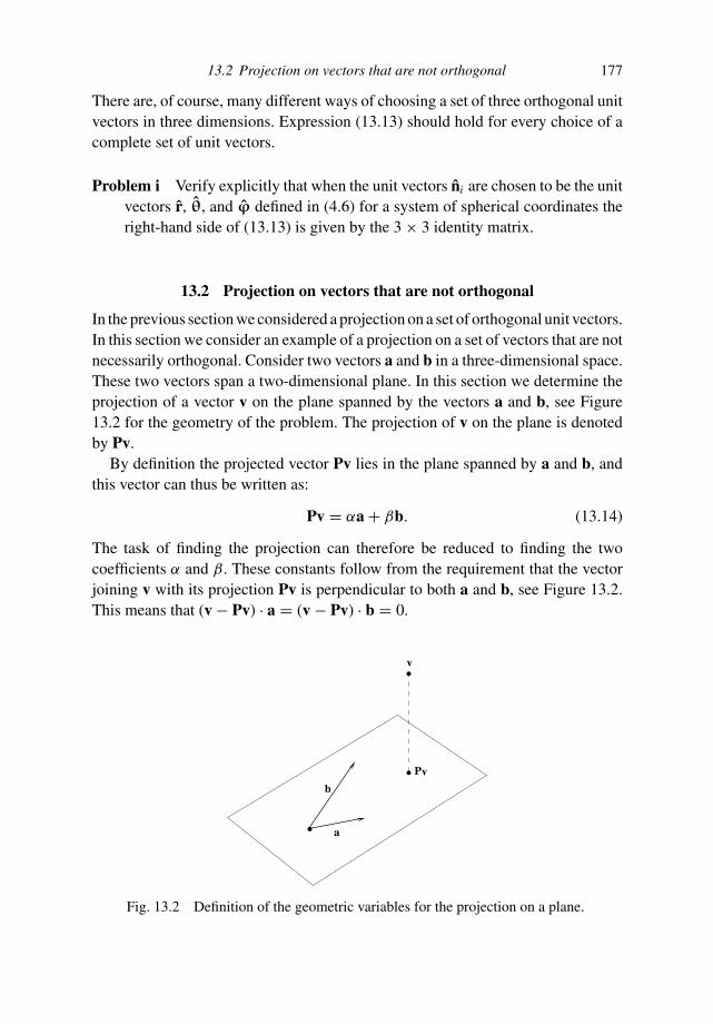
13.2 Projection on vectors that are not orthogonal 177
There are, of course, many different ways of choosing a set of three orthogonal unitvectors in three dimensions. Expression (13.13) should hold for every choice of acomplete set of unit vectors.
Problem i Verify explicitly that when the unit vectors ni are chosen to be the unitvectors r, θ, and ϕ defined in (4.6) for a system of spherical coordinates theright-hand side of (13.13) is given by the 3 × 3 identity matrix.
13.2 Projection on vectors that are not orthogonal
In the previous section we considered a projection on a set of orthogonal unit vectors.In this section we consider an example of a projection on a set of vectors that are notnecessarily orthogonal. Consider two vectors a and b in a three-dimensional space.These two vectors span a two-dimensional plane. In this section we determine theprojection of a vector v on the plane spanned by the vectors a and b, see Figure13.2 for the geometry of the problem. The projection of v on the plane is denotedby Pv.
By definition the projected vector Pv lies in the plane spanned by a and b, andthis vector can thus be written as:
Pv = αa + βb. (13.14)
The task of finding the projection can therefore be reduced to finding the twocoefficients α and β. These constants follow from the requirement that the vectorjoining v with its projection Pv is perpendicular to both a and b, see Figure 13.2.This means that (v − Pv) · a = (v − Pv) · b = 0.
Pv
v
a.
.
.b
Fig. 13.2 Definition of the geometric variables for the projection on a plane.
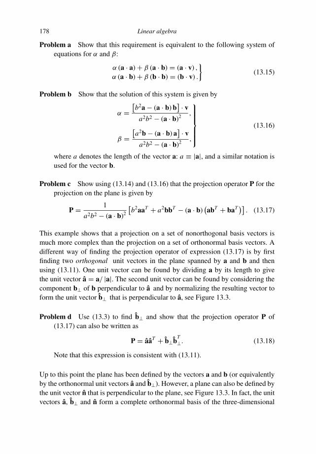
178 Linear algebra
Problem a Show that this requirement is equivalent to the following system ofequations for α and β:
α (a · a) + β (a · b) = (a · v) ,
α (a · b) + β (b · b) = (b · v) .
(13.15)
Problem b Show that the solution of this system is given by
α =[
b2a − (a · b) b] · v
a2b2 − (a · b)2 ,
β =[
a2b − (a · b) a] · v
a2b2 − (a · b)2 ,
⎫
⎪
⎪
⎪
⎪
⎬
⎪
⎪
⎪
⎪
⎭
(13.16)
where a denotes the length of the vector a: a ≡ |a|, and a similar notation isused for the vector b.
Problem c Show using (13.14) and (13.16) that the projection operator P for theprojection on the plane is given by
P = 1
a2b2 − (a · b)2
[
b2aaT + a2bbT − (a · b)(
abT + baT)]
. (13.17)
This example shows that a projection on a set of nonorthogonal basis vectors ismuch more complex than the projection on a set of orthonormal basis vectors. Adifferent way of finding the projection operator of expression (13.17) is by firstfinding two orthogonal unit vectors in the plane spanned by a and b and thenusing (13.11). One unit vector can be found by dividing a by its length to givethe unit vector a = a/ |a|. The second unit vector can be found by considering thecomponent b⊥ of b perpendicular to a and by normalizing the resulting vector toform the unit vector b⊥ that is perpendicular to a, see Figure 13.3.
Problem d Use (13.3) to find b⊥ and show that the projection operator P of(13.17) can also be written as
P = aaT + b⊥bT⊥. (13.18)
Note that this expression is consistent with (13.11).
Up to this point the plane has been defined by the vectors a and b (or equivalentlyby the orthonormal unit vectors a and b⊥). However, a plane can also be defined bythe unit vector n that is perpendicular to the plane, see Figure 13.3. In fact, the unitvectors a, b⊥ and n form a complete orthonormal basis of the three-dimensional
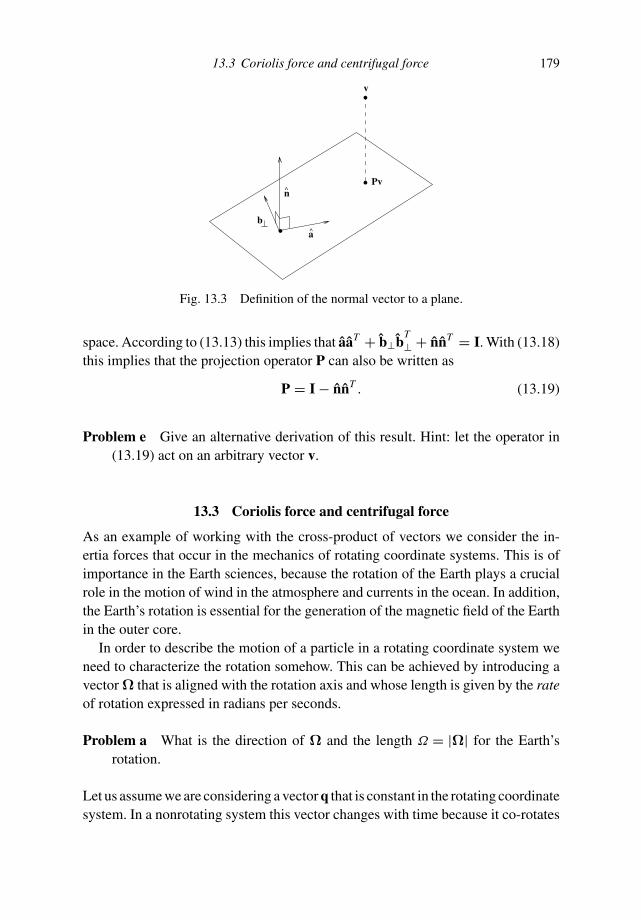
13.3 Coriolis force and centrifugal force 179
b
n^
a
v
.
.
. Pv
Fig. 13.3 Definition of the normal vector to a plane.
space. According to (13.13) this implies that aaT + b⊥bT⊥ + nnT = I. With (13.18)
this implies that the projection operator P can also be written as
P = I − nnT . (13.19)
Problem e Give an alternative derivation of this result. Hint: let the operator in(13.19) act on an arbitrary vector v.
13.3 Coriolis force and centrifugal force
As an example of working with the cross-product of vectors we consider the in-ertia forces that occur in the mechanics of rotating coordinate systems. This is ofimportance in the Earth sciences, because the rotation of the Earth plays a crucialrole in the motion of wind in the atmosphere and currents in the ocean. In addition,the Earth’s rotation is essential for the generation of the magnetic field of the Earthin the outer core.
In order to describe the motion of a particle in a rotating coordinate system weneed to characterize the rotation somehow. This can be achieved by introducing avector Ω that is aligned with the rotation axis and whose length is given by the rateof rotation expressed in radians per seconds.
Problem a What is the direction of Ω and the length Ω = |Ω| for the Earth’srotation.
Let us assume we are considering a vector q that is constant in the rotating coordinatesystem. In a nonrotating system this vector changes with time because it co-rotates
180 Linear algebra
q=
q.b
q
Ω
Fig. 13.4 Decomposition of a vector in a rotating coordinate system.
with the rotating system. The vector q can be decomposed into a component q//
along the rotation vector and a component q⊥ perpendicular to the rotation vector.In addition, a vector b is defined in Figure 13.4 that is perpendicular to both q⊥ andΩ in such a way that Ω, q⊥ and b form a right-handed orthogonal system.
Problem b Show that:
q// = Ω(
Ω · q)
,
q⊥ = q − Ω(
Ω · q)
,
b = Ω × q.
⎫
⎪
⎪
⎬
⎪
⎪
⎭
(13.20)
The last identity follows by inserting the second equation into the identityb = Ω × q⊥.
Problem c In a fixed nonrotating coordinate system, the vector q rotates, hence itsposition is time-dependent: q = q(t). Let us consider how the vector changesover a time interval t . Since the component q// is at all times directedalong the rotation vector Ω, it is constant in time. Over a time interval tthe coordinate system rotates over an angle Ωt . Use this to show that thecomponent of q perpendicular to the rotation vector satisfies:
q⊥(t + t) = cos (Ωt) q⊥(t) + sin (Ωt) b, (13.21)
and that time evolution of q is therefore given by
q(t + t) = q(t) + [cos (Ωt) − 1] q⊥(t) + sin (Ωt) b. (13.22)
13.3 Coriolis force and centrifugal force 181
Problem d The goal is to obtain the time derivative of the vector q. This quantitycan be computed using the rule dq/dt = limt→0[q(t + t) − q(t)]/t . Usethis and (13.22) to show that
q = Ωb, (13.23)
where the dot denotes the time derivative. Use (13.20) to show that the timederivative of the vector q is given by
q = Ω × q. (13.24)
At this point the vector q can be any vector that co-rotates with the rotating coordi-nate system. In this rotating coordinate system, three Cartesian basis vectors x, y,
and z can be used as a basis to decompose the position vector:
rrot = x x + yy + zz. (13.25)
Since these basis vectors are constant in the rotating coordinate system, they satisfy(13.24) so that:
dx/dt = Ω × x,
d y/dt = Ω × y,
d z/dt = Ω × z.
⎫
⎬
⎭
(13.26)
It should be noted that we have not assumed that the position vector rrot in (13.25)rotates with the coordinate system, we have only assumed that the unit vectors x, y,
and z rotate with the coordinate system. Of course, this will leave an imprint on thevelocity and the acceleration. In general the velocity and the acceleration followby differentiating (13.25) with time. If the unit vectors x, y, and z were fixed, theywould not contribute to the time derivative. However, the unit vectors x, y, and zrotate with the coordinate system and the associated time derivative is given by(13.26).
Problem e Differentiate the position vector in (13.25) with respect to time andshow that the velocity vector v is given by:
v = x x + yy + zz + Ω × rrot. (13.27)
The terms x x + yy + zz denote the velocity as seen in the rotating coordinatesystem; this velocity is denoted by vrot. The velocity vector can therefore be writtenas:
v = vrot + Ω × rrot. (13.28)
Problem f Give an interpretation of the last term in this expression.

182 Linear algebra
Problem g The acceleration follows by differentiating (13.27) for the velocityonce more with respect to time. Show that the acceleration is given by
a = x x + yy + zz + 2Ω × (x x + yy + zz) + Ω × (Ω × rrot) . (13.29)
The terms x x + yy + zz on the right-hand side denote the acceleration as seenin the rotating coordinate system; this quantity will be denoted by arot. The termsx x + yy + zz again denote the velocity vrot as seen in the rotating coordinate system.The left-hand side is by Newton’s law equal to F/m, where F is the force acting onthe particle.
Problem h Use this to show that in the rotating coordinate system Newton’s lawis given by:
marot = F − 2mΩ × vrot − mΩ × (Ω × rrot) . (13.30)
The rotation manifests itself through two additional forces. The term −2mΩ × vrot
describes the Coriolis force and the term −mΩ × (Ω × rrot) describes the cen-trifugal force.
Problem i Show that the centrifugal force is perpendicular to the rotation axisand is directed from the rotation axis towards the particle.
Problem j Air flows from high-pressure areas to low-pressure areas. As airflows in the northern hemisphere from a high-pressure area to a low-pressurearea, is it deflected towards the right or towards the left when seen fromabove?
Problem k Compute the magnitude of the centrifugal force and the Coriolis forceyou experience due to the Earth’s rotation when you ride your bicycle. Comparethis with the force mg you experience due to the gravitational attraction of theEarth. It suffices to compute the orders of magnitude of the different terms. Inthe northern hemisphere does the Coriolis force deflect you to the left or tothe right? Have you ever noticed a tilt due to the Coriolis force while ridingyour bicycle?
In meteorology and oceanography it is often convenient to describe the motionof air or water along the Earth’s surface using a Cartesian coordinate system thatrotates with the Earth with unit vectors pointing eastwards (e1), northwards (e2), andupwards (e3), see Figure 13.5. These unit vectors can be related to the unit vectors

13.3 Coriolis force and centrifugal force 183
^e1
^e2
^e 3
Fig. 13.5 Definition of a local Cartesian coordinate system that is aligned withthe Earth’s surface.
r, ϕ and θ that are defined in (4.7). Let the velocity in the eastward direction bedenoted by u, the velocity in the northward direction by v, and the vertical velocityby w.
Problem l Show that:
e1 = ϕ, e2 = −θ, e3 = r, (13.31)
and that the velocity in this rotating coordinate system is given by
v = ue1 + ve2 + we3. (13.32)
Problem m We assume that the axes of the spherical coordinate system are chosenin such a way that the direction θ = 0 is aligned with the rotation axis. Thisis a different way of saying that the rotation vector is parallel to the z-axis:Ω = Ωz. Use the first two expressions of (4.13) to show that the rotation vectorhas the following expansion in terms of the unit vectors r and θ:
Ω = Ω
(
cos θ r − sin θ θ)
. (13.33)
Problem n In the rotating coordinate system, the Coriolis force is given by Fcor =−2mΩ × v. Use expressions (13.31)–(13.33) and (4.11) for the cross-product

184 Linear algebra
of the unit vectors to show that the Coriolis force is given by
Fcor = 2mΩ sin θ u r + 2mΩ cos θ u θ + 2mΩ (v cos θ − w sin θ ) ϕ. (13.34)
Problem o Both the ocean and the atmosphere are shallow in the sense that thevertical length scale (a few kilometers for the ocean and around 10 kilometersfor the atmosphere) is much less than the horizontal length scale. This causesthe vertical velocity to be much smaller than the horizontal velocity. For thisreason the vertical velocity w can be neglected in (13.34). Use this approxi-mation and definition (13.31) to show that the horizontal component aH
cor ofthe Coriolis acceleration is given in this approach by:
aHcor = − f e3 × v, (13.35)
with
f = 2Ω cos θ. (13.36)
This result is widely used in meteorology and oceanography, because (13.35) statesthat, in the Cartesian coordinate system aligned with the Earth’s surface, the Coriolisforce generated by the rotation around the true Earth’s axis of rotation is identicalto the Coriolis force generated by the rotation around a vertical axis with a rotationrate given by Ω cos θ . This rotation rate is largest at the poles, where cos θ = ±1,and vanishes at the equator, where cos θ = 0. The parameter f in (13.35) actsas a coupling parameter; it is called the Coriolis parameter. (In the literature ongeophysical fluid dynamics one often uses latitude rather than the colatitude θ thatis used here, and for this reason one often sees a sin term rather than a cos term inthe definition of the Coriolis parameter.) In many applications one disregards thedependence of f on the colatitude θ ; in that approach f is a constant and one speaksof the f -plane approximation. However, the dependence of the Coriolis parameteron θ is crucial in explaining a number of atmospheric and oceanographic phenomenasuch as the propagation of Rossby waves and the formation of the Gulfstream. Ina further refinement one linearizes the dependence of the Coriolis parameter withcolatitude. This leads to the β-plane approximation. Details can be found in thebooks of Holton [50] and Pedlosky [82].
13.4 Eigenvalue decomposition of a square matrix
In this section we consider the way in which a square N × N matrix A operates ona vector. Since a matrix describes a linear transformation from a vector to a newvector, the action of the matrix A can be quite complicated. However, suppose the

13.4 Eigenvalue decomposition of a square matrix 185
matrix has a set of eigenvectors v(n). We assume these eigenvectors are normalized,hence a caret is used in the notation v(n). These eigenvectors are useful because theaction of A on an eigenvector v(n) is simple:
Av(n) = λn v(n), (13.37)
where λn is the eigenvalue of the eigenvector v(n). When A acts on an eigenvector,the resulting vector is parallel to the original vector, and the only effect of A onthis vector is to elongate the vector (when λn ≥ 1), compress the vector (when0 ≤ λn < 1), or reverse the vector (when λn < 0). We restrict ourselves here tomatrices that are real and symmetric.
Problem a Show that for such a matrix the eigenvalues are real and the eigenvec-tors are orthogonal.
The fact that the eigenvectors v(n) are normalized and mutually orthogonal can beexpressed as
(
v(n) · v(m)) = δnm, (13.38)
where δnm is the Kronecker delta which is defined as
δnm =
1 when n = m0 when n = m
. (11.15)
The eigenvectors v(n) can be used to define the columns of a matrix V:
V =
⎛
⎜
⎜
⎝
......
...v(1) v(2) · · · v(N )
......
...
⎞
⎟
⎟
⎠
; (13.39)
this definition implies that
Vi j ≡ v( j)i . (13.40)
Problem b Use the orthogonality of the eigenvectors v(n) (expression (13.38)) toshow that the matrix V is unitary, that is to show that
VT V = I, (13.41)
where I is the identity matrix with elements Ikl = δkl . The superscript T de-notes the transpose.
186 Linear algebra
There are N eigenvectors which are mutually orthonormal in an N -dimensionalspace. These eigenvectors therefore form a complete set and analogously to (13.13)the completeness relation can be expressed as
I =N
∑
n=1
v(n)v(n)T . (13.42)
When the terms in this expression operate on an arbitrary vector p, an expansionof p in the eigenvectors that is analogous to (13.11) is obtained:
p =N
∑
n=1
v(n)v(n)T p =N
∑
n=1
v(n)(
v(n) · p)
. (13.43)
This is a useful expression because it can be used to simplify the effect of the matrixA on an arbitrary vector p.
Problem c Let A act on (13.43) and show that:
Ap =N
∑
n=1
λn v(n)(
v(n) · p)
. (13.44)
This expression has an interesting geometric interpretation. When A acts on p,the vector p is projected on each of the eigenvectors; this is described by theterm (v(n) · p). The corresponding eigenvector v(n) is multiplied by the eigen-value v(n) → λn v(n), and the result is summed over all the eigenvectors. Theaction of A can thus be reduced to a projection on eigenvectors, a multiplica-tion with the corresponding eigenvalue and a summation over all eigenvectors.The eigenvalue λn can be seen as the sensitivity of the eigenvector v(n) to thematrix A.
Problem d Expression (13.44) holds for every vector p . Use this to show that Acan be written as:
A =N
∑
n=1
λn v(n)v(n)T . (13.45)
Problem e Show that with the definition (13.39) this result can also be writtenas:
A = VVT , (13.46)

13.5 Computing a function of a matrix 187
where is a matrix that has the eigenvalues on its diagonal and whose otherelements are equal to zero:
=
⎛
⎜
⎜
⎜
⎝
λ1 0 · · · 00 λ2 · · · 0...
.... . .
...0 0 λN
⎞
⎟
⎟
⎟
⎠
. (13.47)
Hint: let (13.46) act on an arbitrary vector, use definition (13.40) and see whathappens.
13.5 Computing a function of a matrix
Expansion (13.45) (or equivalently (13.46)) is useful because it provides a way tocompute the inverse of a matrix and to compute functions of a matrix such as theexponential of a matrix. Let us first use ( 13.45) to compute the inverse A−1 of thematrix. In order to do this we must know the effect of A−1 on the eigenvectors v(n).
Problem a Use the identities v(n) = Iv(n) = A−1Av(n) = A−1λn v(n) to show thatv(n) is also an eigenvector of the inverse A−1 with eigenvalue 1/λn:
A−1v(n) = 1
λnv(n). (13.48)
Problem b Use this result and the eigenvector decomposition (13.43) to showthat the effect of A−1 on a vector p can be written as
A−1p =N
∑
n=1
1
λnv(n) (v(n) · p
)
. (13.49)
Also show that this implies that A−1 can also be written as:
A−1 = V−1VT , (13.50)
with
−1 =
⎛
⎜
⎜
⎜
⎝
1/λ1 0 · · · 00 1/λ2 · · · 0...
.... . .
...0 0 1/λN
⎞
⎟
⎟
⎟
⎠
. (13.51)
This is an important result: it means that once we have computed the eigenvectors
188 Linear algebra
and eigenvalues of a matrix, we can compute the inverse matrix efficiently. Notethat this procedure gives problems when one of the eigenvalues is equal to zerobecause for such an eigenvalue 1/λn is not defined. This makes sense: whenone (or more) of the eigenvalues vanishes, the matrix is singular and the inversedoes not exist. Also when one of the eigenvalues is nonzero but close to zero,the corresponding term 1/λn is large, and in practice this gives rise to numeri-cal instabilities. In this situation the inverse of the matrix exists, but the result isvery sensitive to computational (and other) errors. Such a matrix is called poorlyconditioned.
In general, a function of a matrix, such as the exponent of a matrix, is not defined.However, suppose we have a function f (z) that operates on a scalar z and that thisfunction can be written as a power series:
f (z) =∑
p
apz p. (13.52)
For example, when f (z) = exp (z), then f (z) = ∑∞p=0(1/p!)z p. On replacing the
scalar z by the matrix A the power series expansion can be used to define the effectof the function f when it operates on the matrix A:
f (A) ≡∑
p
apAp. (13.53)
Although this may seem to be a simple rule for computing f (A), it is actually notso useful because in many applications the summation (13.53) consists of infinitelymany terms and the computation of Ap can be computationally very demanding.Again, the eigenvalue decomposition (13.45) or (13.46) allows us to simplify theevaluation of f (A).
Problem c Show that v(n) is also an eigenvector of Ap with eigenvalue (λn)p, thatis show that
Apv(n) = (λn)p v(n). (13.54)
Hint: first compute A2v(n) = A(
Av(n)), then A3v(n), etc.
Problem d Use this result to show that (13.46) can be generalized to:
Ap = V pVT , (13.55)

13.6 Normal modes of a vibrating system 189
with p given by
p =
⎛
⎜
⎜
⎜
⎝
λp1 0 · · · 0
0 λp2 · · · 0
......
. . ....
0 0 λpN
⎞
⎟
⎟
⎟
⎠
. (13.56)
Problem e Finally use (13.52) and (13.53) to show that f (A) can be written as:
f (A) = V f () VT , (13.57)
with f () given by
f () =
⎛
⎜
⎜
⎜
⎝
f (λ1) 0 · · · 00 f (λ2) · · · 0...
.... . .
...0 0 f (λN )
⎞
⎟
⎟
⎟
⎠
. (13.58)
Problem f In order to revert to an explicit eigenvector expansion, show that(13.57) can be written as:
f (A) =N
∑
n=1
f (λn) v(n)v(n)T . (13.59)
With this expression (or the equivalent expression (13.57 )) the evaluation of f (A)is simple once the eigenvectors and eigenvalues of A are known, because in (13.59)the function f only acts on the eigenvalues, but not on the matrix. Since the functionf normally acts on a scalar (such as the eigenvalues), the eigenvector decompositionhas obviated the need for computing higher powers of the matrix A. From a numer-ical point of view, however, computing functions of matrices can be a tricky issue.For example, Moler and van Loan [70] give nineteen dubious ways to compute theexponential of a matrix.
13.6 Normal modes of a vibrating system
An eigenvector decomposition is not only useful for computing the inverse of amatrix and other functions of a matrix, it also provides a way to analyze character-istics of dynamical systems. As an example, a simple model for the oscillations ofa vibrating molecule is discussed here. This system is the prototype of a vibratingsystem that has different modes of vibration. The natural modes of vibration are

190 Linear algebra
k1 k2
m1 m2
x2 x
3x1
mm m
Fig. 13.6 Definition of variables for a simple vibrating system.
usually called the normal modes of that system. Consider the mechanical systemshown in Figure 13.6. Three particles with mass m are coupled by two springswith spring constant k. It is assumed that the three masses are constrained to movealong a line. The displacements of the masses from their equilibrium positions aredenoted with x1, x2, and x3. This mechanical model can considered to be a grosslyoversimplified model of a tri-atomic molecule such as CO2 or H2O.
Each of the masses can experience an external force Fi , where the subscript idenotes the mass under consideration. The equations of motion for the three massesare given by:
mx1 = k(x2 − x1) + F1,
mx2 = −k(x2 − x1) + k(x3 − x2) + F2,
mx3 = −k(x3 − x2) + F3.
⎫
⎬
⎭
(13.60)
For the moment we consider harmonic oscillations, that is we assume that boththe driving forces Fi and the displacements xi vary with time as e−iωt . Thedisplacements x1, x2, and x3 can be used to form a vector x, and similarly a vectorF can be formed from the three forces F1, F2, and F3 that act on the three masses.
Problem a Show that for a harmonic motion with frequency ω the equations ofmotion can be written in vector form as:
(
A − mω2
kI)
x = 1
kF, (13.61)
with the matrix A given by
A =⎛
⎝
1 −1 0−1 2 −1
0 −1 1
⎞
⎠ . (13.62)
The normal modes of the system are given by the patterns of oscillations of thesystem when there is no driving force. For this reason, we set the driving forceF on the right-hand side of (13.61) momentarily to zero. Equation (13.61) thenreduces to a homogeneous system of linear equations; such a system of equationscan only have nonzero solutions when the determinant of the matrix vanishes.Since the matrix A has three eigenvalues, the system can only oscillate freely at

13.6 Normal modes of a vibrating system 191
three discrete eigenfrequencies. The system can only oscillate at other frequencieswhen it is driven by the force F at such a frequency.
Problem b Show that the eigenfrequencies ωi of the vibrating system are givenby
ωi =√
kλi
m, (13.63)
where λi are the eigenvalues of the matrix A.
Problem c Show that the eigenfrequencies of the system are given by:
ω1 = 0, ω2 =√
k
m, ω3 =
√
3k
m. (13.64)
Problem d The frequencies do not give the vibrations of each of the three particlesrespectively. Instead these frequencies give the eigenfrequencies of the threemodes of oscillation of the system. The eigenvector that corresponds to eacheigenvalue gives the displacement of each particle for that mode of oscillation.Show that these eigenvectors are given by:
v(1) = 1√3
⎛
⎝
111
⎞
⎠ , v(2) = 1√2
⎛
⎝
10
−1
⎞
⎠ , v(3) = 1√6
⎛
⎝
1−21
⎞
⎠ . (13.65)
Remember that the eigenvectors can be multiplied by an arbitrary constant,and this constant is chosen in such a way that each eigenvector has length 1.
Problem e Show that these eigenvectors satisfy the requirement (13.38).
Problem f Sketch the motion of the three masses for each normal mode. Explainphysically why the third mode with frequency ω3 has a higher eigenfrequencythan the second mode ω2.
Problem g Explain physically why the second mode has an eigenfrequency ω2 =√k/m that is identical to the frequency of a single mass m that is suspended
by a spring with spring constant k.
Problem h What type of motion does the first mode with eigenfrequency ω1
describe? Explain physically why this frequency is independent of the springconstant k and the mass m.

192 Linear algebra
Now that we know the normal modes of the system, we consider the case inwhich the system is driven by a force F that varies in time as e−iωt . For sim-plicity it is assumed that the frequency ω of the driving force differs from theeigenfrequencies of the system: ω = ωi . The eigenvectors v(n) defined in (13.65)form a complete orthonormal set, hence both the driving force F and the dis-placement x can be expanded in this set. Using ( 13.43) the driving force can beexpanded as
F =3
∑
n=1
v(n)(v(n) · F). (13.66)
Problem i Write the displacement vector as a superposition of the normal modedisplacements: x = ∑3
n=1 cn v(n), use expansion (13.66) for the driving forceand insert these equations in the equation of motion (13.61) to solve for theunknown coefficients cn . Eliminate the eigenvalues with (13.63) in favour ofthe eigenfrequencies ωn , and show that the displacement is given by:
x = 1
m
3∑
n=1
v(n)(v(n) · F)(
ω2n − ω2
) . (13.67)
This expression has a nice physical interpretation. Expression ( 13.67) states thatthe total response of the system can be written as a superposition of the differentnormal modes (the
∑3n=1 v(n) terms). The effect that the force has on each normal
mode is given by the inner product (v(n) · F). This is nothing but the componentof the force F along the eigenvector v(n), see (13.2). The term 1/
(
ω2n − ω2
)
givesthe sensitivity of each mode to a driving force with frequency ω; this term can becalled a sensitivity term. When the driving force is close to one of the eigenfre-quencies of the nth mode, 1/
(
ω2n − ω2
)
is large. In that case the system is closeto resonance and the resulting displacement is large. On the other hand, whenthe frequency of the driving force is far from the eigenfrequencies of the system,1/
(
ω2n − ω2
)
is small and the system gives a small response. The total responsecan be seen as a combination of three basic operations: eigenvector expansion,projection, and multiplication with a response function. Note that the same op-erations were used in the explanation of the action of a matrix A given belowequation (13.44).
13.7 Singular value decomposition
In Section 13.4 the decomposition of a square matrix in terms of eigenvectors wastreated. In many practical applications, such as inverse problems, one encounters a
13.7 Singular value decomposition 193
system of equations that is not square:
A︸︷︷︸
M × Nmatrix
x︸︷︷︸
Nrows
= y︸︷︷︸
Mrows
(13.68)
Consider the example in which the vector x has N components and there are Mequations. In that case the vector y has M components and the matrix A has Mrows and N columns, that is it is an M × N matrix. A relation such as (13.37)which states that Av(n) = λn v(n) cannot possibly hold because when the matrix Aacts on an N -vector it produces an M-vector, whereas in (13.37) the vector on theright-hand side has the same number of components as the vector on the left-handside. It is clear that the theory of Section 13.4 cannot be applied when the matrix isnot square. However, it is possible to generalize the theory of Section 13.4 when Ais not square. For simplicity it is assumed that A is a real matrix.
In Section 13.4 a single set of orthonormal eigenvectors v(n) was used to analyzethe problem. Since the vectors x and y in (13.68) have different dimensions, it isnecessary to expand the vector x in a set of N orthogonal vectors v(n) that each haveN components and to expand y in a different set of M orthogonal vectors u(m) thateach have M components. Suppose we have chosen a set v(n), let us define vectorsu(n) by the following relation:
Av(n) = λnu(n). (13.69)
The constant λn should not be confused with an eigenvalue, this constant followsfrom the requirement that v(n) and u(n) are both vectors of unit length. At this point,the choice of v(n) is still open. The vectors v(n) will now be required to satisfy inaddition to (13.69) the following condition:
AT u(n) = µn v(n), (13.70)
where AT is the transpose of A.
Problem a In order to find the vectors v(n) and u(n) that satisfy both (13.69) and(13.70), multiply (13.69) by AT and use (13.70) to eliminate u(n). Do this toshow that v(n) satisfies:
(
AT A)
v(n) = λnµn v(n). (13.71)
Use similar steps to show that u(n) satisfies(
AAT)
u(n) = λnµnu(n). (13.72)

194 Linear algebra
These equations state that the v(n) are the eigenvectors of AT A and that the u(n) arethe eigenvectors of AAT .
Problem b Show that both AT A and AAT are real symmetric matrices and thatthis implies that the basis vectors v(n) (n = 1, . . . , N ) and u(m) (m = 1, . . . , M)are both orthonormal:
(
v(n) · v(m)) = (
u(n) · u(m)) = δnm . (13.73)
Although (13.71) and (13.72) can be used to find the basis vectors v(n) and u(n),these expressions cannot be used to find the constants λn and µn , because they statethat the product λnµn is equal to the eigenvalues of AT A and AAT . This impliesthat only the product of λn and µn is defined.
Problem c In order to find the relation between λn and µn , take the inner productof (13.69) with u(n) and use the orthogonality relation (13.73) to show that:
λn = (
u(n) · Av(n)) . (13.74)
Problem d Show that for arbitrary vectors p and q
(p · Aq) = (
AT p · q)
. (13.75)
Problem e Apply this relation to (13.74) and use (13.70) to show that
λn = µn. (13.76)
This is all the information we need to find both λn and µn . Since these quantitiesare equal, and since by virtue of ( 13.71) these eigenvectors are equal to the eigen-vectors of AT A, it follows that both λn and µn are given by the square-root of theeigenvalues of AT A. Note that it follows from (13.72) that the product λnµn alsoequals the eigenvalues of AAT . This can only be the case when AT A and AAT havethe same eigenvalues. Before we proceed, let us show that this is indeed true. Letthe eigenvalues of AT A be denoted by Λn and the eigenvalues of AAT by Υn , thatis
AT Av(n) = Λn v(n) (13.77)
and
AAT u(n) = Υnu(n). (13.78)
13.7 Singular value decomposition 195
Problem f Take the inner product of (13.77) with v(n) to show that Λn = (v(n) ·AT Av(n)), use the properties (13.75) and AT T = A and (13.69) to show thatλ2
n = Λn . Use similar steps to show that µ2n = Υn . With ( 13.76) this implies
that AAT and AT A have the same eigenvalues.
The proof that AAT and AT A have the same eigenvalues was not only given asa check of the consistency of the theory, the fact that AAT and AT A have thesame eigenvalues has important implications. Since AAT is an M × M matrix,it has M eigenvalues, and since AT A is an N × N matrix it has N eigenval-ues. The only way for these matrices to have the same eigenvalues, but to havea different number of eigenvalues is for the number of nonzero eigenvalues tobe given by the minimum of N and M . In practice, some of the eigenvaluesof AAT may be zero, hence the number of nonzero eigenvalues of AAT can beless than M . By the same token, the number of nonzero eigenvalues of AT A canbe less than N . The number of nonzero eigenvalues will be denoted by P . It isnot known a priori how many nonzero eigenvalues there are, but it follows fromthe arguments above that P is smaller than or equal to M and N . This impliesthat
P ≤ min(N , M), (13.79)
where min(N , M) denotes the minimum of N and M . Therefore, whenever a sum-mation over eigenvalues occurs, we need to take only P eigenvalues into account.Since the ordering of the eigenvalues is arbitrary, it is assumed in the followingthat the eigenvectors are ordered in decreasing size: λ1 ≥ λ2 ≥ · · · ≥ λP . In thisordering the eigenvalues for n > P are equal to zero so that the summation overeigenvalues runs from 1 to P .
Problem g The matrices AAT and AT A have the same eigenvalues. When youneed the eigenvalues and eigenvectors, from the point of view of computa-tional efficiency would it be more efficient to compute the eigenvalues andeigenvectors of AT A or of AAT ? Consider the situations M > N and M < Nseparately.
Let us now return to the task of making an eigenvalue decomposition of the ma-trix A. The vectors v(n) form a basis in N -dimensional space. Since the vectorx is N -dimensional, every vector x can be decomposed according to (13.43):x = ∑N
n=1 v(n)(v(n) · x).

196 Linear algebra
Problem h Let the matrix A act on this expression and use ( 13.69) to show that:
Ax =P
∑
n=1
λnu(n)(
v(n) · x)
. (13.80)
Problem i This expression must hold for any vector x. Use this property to deducethat:
A =P
∑
n=1
λnu(n)v(n)T . (13.81)
Problem j The eigenvectors v(n) can be arranged in an N × N matrix V, definedin (13.39). Similarly the eigenvectors u(n) can be used to form the columns ofan M × M matrix U:
U =
⎛
⎜
⎜
⎝
......
...u(1) u(2) · · · u(M)
......
...
⎞
⎟
⎟
⎠
. (13.82)
Show that A can also be written as:
A = UVT , (13.83)
with the diagonal matrix defined in (13.47).
This decomposition of A in terms of eigenvectors is called the singular valuedecomposition of the matrix. This is frequently abbreviated to SVD.
Problem k You may have noticed the similarity between (13.81 ) and (13.45)for a square matrix and (13.83) and (13.46). Show that for the special caseM = N the theory of this section is identical to the eigenvalue decompositionfor a square matrix presented in Section 13.4. Hint: what are the vectors u(n)
when M = N?
Let us now solve the original system of linear equations (13.68) for the unknownvector x. In order to do this, expand the vector y in the vectors u(n) that span the M-dimensional space: y = ∑M
m=1 u(m)(u(m) · y), and expand the vector x in the vectorsv(n) that span the N -dimensional space:
x =N
∑
n=1
cn v(n). (13.84)

13.8 Householder transformation 197
Problem l At this point the coefficients cn are unknown. Insert the expansionsfor y and x and the expansion (13.81) for the matrix A in the linear system(13.68) and use the orthogonality properties of the eigenvectors to show thatcn = (u(n) · y)/λn , so that
x =P
∑
n=1
1
λn
(
u(n) · y)
v(n). (13.85)
Note that although in the original expansion (13.84) a summation is carried outover all N basis vectors, in solution (13.85) a summation is carried out over thefirst P basis vectors only. The reason for this is that the remaining eigenvectorshave eigenvalues that are equal to zero so that they can be left out of the expansion(13.81) of the matrix A. Indeed, these eigenvalues would give rise to problemsbecause if they were retained they would lead to infinite contributions 1/λ → ∞ insolution (13.85). In practice, some eigenvalues may be nonzero, but close to zero,so that the term 1/λ gives rise to numerical instabilities. Therefore, one also oftenleaves out nonzero but small eigenvalues in summation (13.85).
This may appear to be an objective procedure for defining solutions for linearproblems that are undetermined or for problems that are otherwise ill-conditioned,but there is a price one pays for leaving out basis vectors in the construction ofthe solution. The vector x is N -dimensional, hence one needs N basis vectors toconstruct an arbitrary vector x, see (13.84). The solution vector given in (13.85)is built by superposing only P basis vectors. This implies that the solution vectoris constrained to be within the P-dimensional subspace spanned by the first Peigenvectors. Therefore, it is not clear that the solution vector in (13.85) is identicalto the true vector x. However, the point of using the singular value decompositionis that the solution is only constrained by the linear system of (13.68 ) within thesubspace spanned by the first P basis vectors v(n). Solution (13.85) ensures thatonly the components of x within that subspace are affected by the right-hand sidevector y . This technique is useful in the analysis of linear inverse problems [79].
13.8 Householder transformation
Linear systems of equations can be solved in a systematic way by sweeping columnsof the matrix that defines the system of equations. As an example consider the system
x + y + 3z = 5,
−x + 2z = 1,
2x + y + 2z = 5.
⎫
⎬
⎭
(13.86)
198 Linear algebra
This system of equations will be written here also as:⎛
⎝
1 1 3 | 5−1 0 2 | 1
2 1 2 | 5
⎞
⎠ , (13.87)
which is nothing but a compressed notation of (13.86). The matrix shown in (13.87)is called the augmented matrix because the matrix defining the left-hand side of(13.86) is augmented with the right-hand side of (13.86). The linear equations canbe solved by adding the first row to the second row and subtracting the first rowtwice from the third row, the resulting system of equations is then represented bythe following augmented matrix:
⎛
⎝
1 1 3 | 50 1 5 | 60 −1 −4 | −5
⎞
⎠ . (13.88)
Note that in the first column all elements below the first elements are equal to zero.By adding the second row to the third row we can also make all elements below thesecond element in the second column equal to zero:
⎛
⎝
1 1 3 | 50 1 5 | 60 0 1 | 1
⎞
⎠ . (13.89)
The system is now in upper-triangular form; this is a different way of sayingthat all matrix elements below the diagonal vanish. This is convenient because thesystem can now be solved by backsubstitution. To see how this works note thatthe augmented matrix (13.89) is a shorthand notation for the following system ofequations:
x + y + 3z = 5,
y + 5z = 6,
z = 1 .
⎫
⎬
⎭
(13.90)
The value of z follows from the last equation, given this value of z the value of yfollows from the middle equations, and given y and z the value of x follows fromthe top equation.
Problem a Show that the solution of the linear equations is given by x = y =z = 1.
For small systems of linear equations this process for solving linear equationscan be carried out by hand. For large systems of equations this process must be

13.8 Householder transformation 199
carried out on a computer. This is only possible when one has a systematic andefficient way of carrying out this sweeping process. Suppose we have an N × Nmatrix A:
A =
⎛
⎜
⎜
⎜
⎝
a11 a12 · · · a1N
a21 a22 · · · a2N...
.... . .
...aN1 aN2 · · · aN N
⎞
⎟
⎟
⎟
⎠
. (13.91)
We want to find an operator Q such that when A is multiplied by Q all elements inthe first column are zero except the element on the diagonal, that is we want to findQ such that:
QA =
⎛
⎜
⎜
⎜
⎝
a′11 a′
12 · · · a′1N
0 a′22 · · · a′
2N...
.... . .
...0 a′
N2 · · · a′N N
⎞
⎟
⎟
⎟
⎠
. (13.92)
This problem can be formulated slightly differently, suppose we denote the firstcolumns of A by the vector u:
u ≡
⎛
⎜
⎜
⎜
⎝
a11
a21...
aN1
⎞
⎟
⎟
⎟
⎠
. (13.93)
The operator Q that we want to find maps this vector to a new vector which onlyhas a nonzero component in the first element:
Qu =
⎛
⎜
⎜
⎜
⎝
a′11
0...0
⎞
⎟
⎟
⎟
⎠
= a′11e1, (13.94)
where e1 is the unit vector in the x1-direction:
e1 ≡
⎛
⎜
⎜
⎜
⎝
10...0
⎞
⎟
⎟
⎟
⎠
. (13.95)

200 Linear algebra
v
n
n(n v ).^^
Qv
v
Fig. 13.7 Geometrical interpretation of the Householder transformation.
The desired operator Q can be found with a so-called Householder transforma-tion. For a given unit vector n the Householder transformation is defined by:
Q ≡ I − 2nnT . (13.96)
Problem b Show that the Householder transformation can be written asQ = I − 2P, where P is the operator for projection along n.
Problem c It follows from (13.3) that any vector v can be decomposed into acomponent along n and a perpendicular component: v = n (n · v) + v⊥. Showthat after the Householder transformation the vector is given by:
Qv = −n (n · v) + v⊥. (13.97)
Problem d Convince yourself that the Householder transformation of v is cor-rectly shown in Figure 13.7.
Problem e Use (13.97) to show that Q does not change the length of a vector.Use this result to show that a′
11 in (13.94) is given by a′11 = |u|.
With (13.94) this means that the Householder transformation should satisfy
Qu = |u| e1. (13.98)
Our goal is now to find a unit vector n such that this expression is satisfied.

13.8 Householder transformation 201
Problem f Use (13.96) to show that if Q satisfies the requirement (13.98) n mustsatisfy the following equation:
2n (n · u) = u − e1; (13.99)
in this expression u is the unit vector in the direction u.
Problem g Equation (13.99) implies that n is directed in the direction of the vectoru − e1, therefore n can be written as n = C (u − e1), with C an undeterminedconstant. Show that (13.98) implies that C = 1/
√2 [1 − (u · e1)]. Also show
that this value of C indeed leads to a vector n that is of unit length.
This value of C implies that the unit vector n to be used in the Householder trans-formation (13.96) is given by
n = u − e1√2 [1 − (u · e1)]
. (13.100)
To see how the Householder transformation can be used to render the matrix el-ements below the diagonal equal to zero apply the transformation Q to the linearequation Ax = y.
Problem h Show that this leads to a new system of equations given by⎛
⎜
⎜
⎜
⎝
|u| a′12 · · · a′
1N
0 a′22 · · · a′
2N...
.... . .
...0 a′
N2 · · · a′N N
⎞
⎟
⎟
⎟
⎠
x = Qy. (13.101)
A second Householder transformation can now be applied to render all elementsin the second column below the diagonal element a′
22 equal to zero. In this way,all the columns of A can be successively swiped. Note that in order to apply theHouseholder transformation one only needs to compute (13.100) and (13.96) tocarry out a matrix multiplication. These operations can be carried out efficiently oncomputers.

14
Dirac delta function
14.1 Introduction of the delta function
In linear algebra, the identity matrix I plays a central role. This operator maps anyvector v onto itself:
Iv = v. (14.1)
This expression can also be written in component form as∑
j
Ii jv j = vi . (14.2)
The identity matrix has diagonal elements that are equal to unity and its off-diagonalelements are equal to zero. This means that the elements of the identity matrix areequal to the Kronecker delta Ii j = δi j , which is defined as:
δi j ≡
1 for i = j0 for i = j
. (14.3)
Expression (14.2) shows that when the identity matrix Ii j acts on all the com-ponents v j of a vector, it selects the component vi . The question we address inthis chapter is: how can this idea be generalized to continuous functions insteadof vectors? In other words, can we find a function I (x0, x) such that when it isintegrated with a function f (x) it selects that function as the location x0:
∫
I (x0, x) f (x)dx = f (x0)? (14.4)
Note the resemblance between this expression and (14.2) for a vector. The vector vis replaced by the function f , the summation over j is changed into the integrationover x, and the index i in (14.2) corresponds to the value x0 in (14.4).
202

14.1 Introduction of the delta function 203
As a first guess for the operator I (x0, x) let us consider the following general-ization of the definition (14.3) of the Kronecker delta to continuous functions:
I (x0, x)?≡
1 for x0 = x0 for x0 = x
. (14.5)
This is not a very good guess; when I (x0, x) is viewed as a function of x , I (x0, x) isalmost everywhere equal to zero except when x = x0. When we integrate I (x0, x)over x the integrand is zero except at the point x = x0, but this point gives avanishing contribution to the integral because the “width” of this point is equal tozero. (Mathematically one would say that a point has zero measure.) This meansthat the integral of I (x0, x) can only give a finite result when I (x0, x) is infinite atx = x0.
As an improved guess let us therefore try the definition
I (x0, x)?≡
∞ for x0 = x0 for x0 = x
. (14.6)
This is not a very precise definition because it is not clear what we mean by “∞”.However, we can learn something from this naive guess because it shows thatI (x0, x) is not a well-behaved function. It is discontinuous at x = x0 and its valueis infinite at that point. It is clear from this that whatever definition of I (x0, x) weuse, it will not lead to a well-behaved function.
A useful definition of I (x0, x) can be obtained from the boxcar function Ba(x)which is defined as
Ba(x) ≡
⎧
⎪
⎨
⎪
⎩
1
2afor |x | ≤ a
0 for |x | > a
. (14.7)
This function is shown for three values of the parameter a in Figure 14.1. (A boxcaris the rectangular railroad car that is used for carrying freight, and the function Ba(x)
–2 –1 1 2x
1
2
3
4
5
6
a = 0.1
a = 0.3a = 1.0
Fig. 14.1 The boxcar function Ba(x) for a = 1.0 (dashed line), a = 0.3 (thinsolid line), and a = 0.1 (thick solid line).

204 Dirac delta function
is called the boxcar function because it has the same rectangular shape as the boxcarused by the railways.)
Problem a Show that∫ ∞
−∞Ba(x)dx = 1. (14.8)
Let us now center the boxcar at a location x0, multiply it by f (x) and integrateover x .
Problem b Use the definition of the boxcar function to derive that∫ ∞
−∞Ba(x − x0) f (x)dx = 1
2a
∫ x0+a
x0−af (x) dx . (14.9)
Pay attention to the limits of integration on the right-hand side.
The integral on the right-hand side is nothing but the average of the function f (x)over the interval (x0 − a, x0 + a) because the pre-factor 1/2a corrects for the widthof that interval. This is a useful expression; as the parameter a goes to zero theintegral (14.9) gives the function at location x0 because the limit a ↓ 0 gives themean value of f (x) over the interval (x0 − 0, x0 + 0). This means that
lima↓0
∫ ∞
−∞Ba(x − x0) f (x) dx = f (x0). (14.10)
This means that this limit has the desired properties of the identity operator I (x0, x)for continuous functions. It is customary to denote this operator as δ(x − x0) andto call it the Dirac delta function. (Usually one refers to this function simply as the“delta function.”) This means that the delta function satisfies the following property:
∫ ∞
−∞δ(x − x0) f (x) dx = f (x0). (14.11)
A comparison of this expression with (14.10) suggests that
δ(x − x0)“ = ” lima↓0
Ba(x − x0). (14.12)
Consider Figure 14.1 again. It can be seen from that figure and definition (14.7)that as a goes to zero, the value of the boxcar function becomes infinite and that thewidth of the boxcar goes to zero. In this sense the limit on the right-hand side doesnot exist, and for this reason the = sign is placed between quotes. The word “deltafunction” is really a misnomer because this “function” is not a function at all. Itsvalue is not defined and it is only nonzero in a region with measure zero. However,
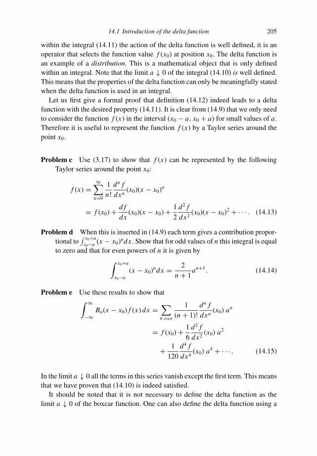
14.1 Introduction of the delta function 205
within the integral (14.11) the action of the delta function is well defined, it is anoperator that selects the function value f (x0) at position x0. The delta function isan example of a distribution. This is a mathematical object that is only definedwithin an integral. Note that the limit a ↓ 0 of the integral (14.10) is well defined.This means that the properties of the delta function can only be meaningfully statedwhen the delta function is used in an integral.
Let us first give a formal proof that definition (14.12) indeed leads to a deltafunction with the desired property (14.11). It is clear from (14.9) that we only needto consider the function f (x) in the interval (x0 − a, x0 + a) for small values of a.Therefore it is useful to represent the function f (x) by a Taylor series around thepoint x0.
Problem c Use (3.17) to show that f (x) can be represented by the followingTaylor series around the point x0:
f (x) =∞
∑
n=0
1
n!
dn f
dxn(x0)(x − x0)n
= f (x0) + d f
dx(x0)(x − x0) + 1
2
d2 f
dx2(x0)(x − x0)2 + · · · . (14.13)
Problem d When this is inserted in (14.9) each term gives a contribution propor-tional to
∫ x0+ax0−a (x − x0)ndx . Show that for odd values of n this integral is equal
to zero and that for even powers of n it is given by∫ x0+a
x0−a(x − x0)ndx = 2
n + 1an+1. (14.14)
Problem e Use these results to show that∫ ∞
−∞Ba(x − x0) f (x) dx =
∑
n even
1
(n + 1)!
dn f
dxn(x0) an
= f (x0) + 1
6
d2 f
dx2(x0) a2
+ 1
120
d4 f
dx4(x0) a4 + · · · . (14.15)
In the limit a ↓ 0 all the terms in this series vanish except the first term. This meansthat we have proven that (14.10) is indeed satisfied.
It should be noted that it is not necessary to define the delta function as thelimit a ↓ 0 of the boxcar function. One can also define the delta function using a
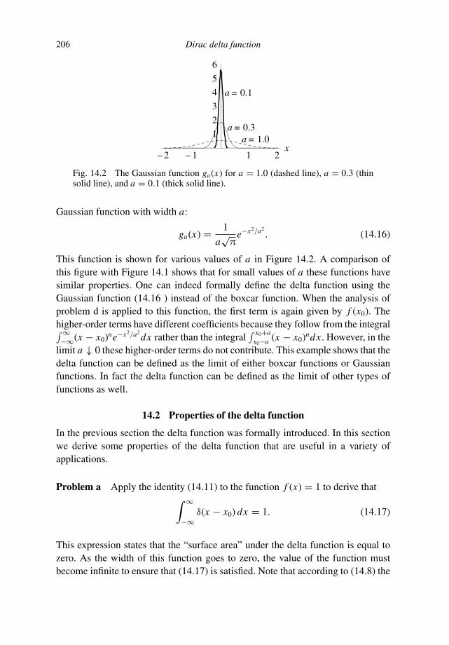
206 Dirac delta function
– 2 – 1 1 2x
1
2
3
4
5
6
a = 0.1
a = 0.3a = 1.0
Fig. 14.2 The Gaussian function ga(x) for a = 1.0 (dashed line), a = 0.3 (thinsolid line), and a = 0.1 (thick solid line).
Gaussian function with width a:
ga(x) = 1
a√
πe−x2/a2
. (14.16)
This function is shown for various values of a in Figure 14.2. A comparison ofthis figure with Figure 14.1 shows that for small values of a these functions havesimilar properties. One can indeed formally define the delta function using theGaussian function (14.16 ) instead of the boxcar function. When the analysis ofproblem d is applied to this function, the first term is again given by f (x0). Thehigher-order terms have different coefficients because they follow from the integral∫ ∞−∞(x − x0)ne−x2/a2
dx rather than the integral∫ x0+a
x0−a (x − x0)ndx . However, in thelimit a ↓ 0 these higher-order terms do not contribute. This example shows that thedelta function can be defined as the limit of either boxcar functions or Gaussianfunctions. In fact the delta function can be defined as the limit of other types offunctions as well.
14.2 Properties of the delta function
In the previous section the delta function was formally introduced. In this sectionwe derive some properties of the delta function that are useful in a variety ofapplications.
Problem a Apply the identity (14.11) to the function f (x) = 1 to derive that∫ ∞
−∞δ(x − x0) dx = 1. (14.17)
This expression states that the “surface area” under the delta function is equal tozero. As the width of this function goes to zero, the value of the function mustbecome infinite to ensure that (14.17) is satisfied. Note that according to (14.8) the

14.2 Properties of the delta function 207
boxcar function Ba(x) that we used to define the delta function indeed satisfies thisproperty.
Problem b Show that the integral of the Gaussian function defined in (14.16) isalso equal to unity:
∫ ∞
−∞ga(x) dx = 1. (14.18)
In this derivation you can use that∫ ∞−∞ e−y2
dy = √π. This means that when
the delta function is defined as the limit a ↓ 0 of the Gaussian function ga(x)property (14.17) is indeed satisfied.
For the next property we consider the delta function δ (c(x − x0)), where c is aconstant. Let us first consider the case in which c is positive.
Problem c Make the substitution y = cx to derive the following identity:∫ ∞
−∞δ (c (x − x0)) f (x) dx =
∫ ∞
−∞δ (y − cx0) f (y/c)
1
cdy. (14.19)
Problem d Carry out the y-integration using property (14.11 ) of the delta func-tion to show that
∫ ∞
−∞δ (c (x − x0)) f (x) dx = 1
cf (x0) (positive c). (14.20)
Problem e Carry out the same analysis for negative values of the constant c, andshow that (14.19) in that case is given by
∫ ∞
−∞δ (c (x − x0)) f (x) dx =
∫ −∞
+∞δ (y − cx0) f (y/c)
1
cdy. (14.21)
Explain why the integration runs from +∞ to −∞.
Problem f When the integration limits in the last integral are reversed, the integralobtains an additional minus sign. Carry out the y-integration and derive that
∫ ∞
−∞δ (c (x − x0)) f (x) dx = − 1
cf (x0) (negative c). (14.22)
For negative values of c, one can use that −c = |c|. For positive values of c,obviously c = |c|. This means that (14.20) and (14.21) can be combined in the
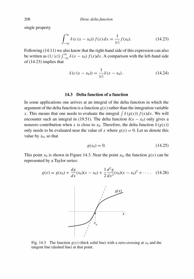
208 Dirac delta function
single property∫ ∞
−∞δ (c (x − x0)) f (x) dx = 1
|c| f (x0). (14.23)
Following (14.11) we also know that the right-hand side of this expression can alsobe written as (1/ |c|) ∫ ∞
−∞ δ (x − x0) f (x)dx . A comparison with the left-hand sideof (14.23) implies that
δ (c (x − x0)) = 1
|c|δ (x − x0) . (14.24)
14.3 Delta function of a function
In some applications one arrives at an integral of the delta function in which theargument of the delta function is a function g(x) rather than the integration variablex . This means that one needs to evaluate the integral
∫
δ (g(x)) f (x)dx . We willencounter such an integral in (19.51). The delta function δ(x − x0) only gives anonzero contribution when x is close to x0. Therefore, the delta function δ (g(x))only needs to be evaluated near the value of x where g(x) = 0. Let us denote thisvalue by x0, so that
g(x0) = 0. (14.25)
This point x0 is shown in Figure 14.3. Near the point x0, the function g(x) can berepresented by a Taylor series:
g(x) = g(x0) + dg
dx(x0)(x − x0) + 1
2
d2g
dx2(x0)(x − x0)2 + · · · . (14.26)
x
x
g(x)
0
Fig. 14.3 The function g(x) (thick solid line) with a zero-crossing at x0 and thetangent line (dashed line) at that point.

14.3 Delta function of a function 209
Because x0 gives the zero-crossing of g(x), see (14.25), the first term is equalto zero. Ignoring the second order term and all higher order terms then givesthe following first order approximation for the function g(x) near its zero-crossing:
g(x) = dg
dx(x0)(x − x0). (14.27)
Problem a Show that the right-hand side of (14.27) describes the straight linethat is tangent to the curve g(x) at the zero crossing x0. This tangent line isshown as the dashed line in Figure 14.3.
Problem b Using this relation one finds that∫
δ (g(x)) f (x) dx =∫
δ
(
dg
dx(x0)(x − x0)
)
f (x) dx . (14.28)
The derivative dg/dx at the point x0 can be considered to be a constant. Usethe results of the previous section to derive that
∫
δ (g(x)) f (x) dx =∫
1∣
∣
∣
∣
dg
dx(x0)
∣
∣
∣
∣
δ(x − x0) f (x) dx, (14.29)
and show that this gives∫
δ (g(x)) f (x) dx = 1∣
∣
∣
∣
dg
dx(x0)
∣
∣
∣
∣
f (x0). (14.30)
Problem c Insert (14.11) into the right-hand side of (14.30) to derive the followingproperty of the delta function
δ (g(x)) = 1∣
∣
∣
∣
dg
dx(x0)
∣
∣
∣
∣
δ(x − x0), (14.31)
where it must be kept in mind that x0 denotes the zero-crossing of g(x).
When the function g(x) has more than one zero-crossing, the analysis of this sec-tion can be applied to each of these zero-crossings. The contributions of all thedifferent zero-crossings must be added because all the points where g(x) = 0 givea contribution to the integral. This means that when the zero-crossings are denoted
210 Dirac delta function
by xi (so that g(xi ) = 0):
δ (g(x)) =∑
i
1∣
∣
∣
∣
dg
dx(xi )
∣
∣
∣
∣
δ(x − xi ). (14.32)
14.4 Delta function in more dimensions
The delta function has been defined for functions of a single variable. Its definitioncan be extended to functions of more variables. As an example we consider herethe delta function in three dimensions. The delta function is then defined as theproduct of the delta functions for each of the coordinates:
δ(r − r0) ≡ δ (x − x0) δ (y − y0) δ (z − z0) . (14.33)
This definition of the delta function can be used in the integral∫
δ(r − r0) f (r) dV .
Problem a Write the volume integral as dV = dxdydz, insert (14.33) and carryout the integration over x to show that
∫
δ(r − r0) f (r) dV =∫
δ (y − y0) δ (z − z0) f (x0, y, z) dydz, (14.34)
paying attention to the arguments of the function f .
Problem b Carry out the y-integration and then the z-integration to derive that∫
δ(r − r0) f (r) dV = f (x0, y0, z0). (14.35)
The right-hand side of (14.35) is the function f at location r0. This means that themulti-dimensional delta function defined in (14.33) satisfies the following property
∫
δ(r − r0) f (r) dV = f (r0). (14.36)
This expression generalizes (14.11) to more dimensions.
14.5 Delta function on the sphere
Up to this point we have analyzed the delta function in Cartesian coordinates. Whenthe delta function is used in a coordinate system that is not Cartesian, additionalterms appear in the definition of the delta function. This is illustrated in this sectionwith the delta function on a sphere. Suppose we define a function f (θ, ϕ) on theunit sphere. Using definition (14.11) the action of the delta function on the sphere

14.5 Delta function on the sphere 211
as expressed in the angles θ and ϕ can be written as∫ 2π
0
∫ π
0δ(θ − θ0)δ(ϕ − ϕ0) f (θ, ϕ) dθdϕ = f (θ0, ϕ0). (14.37)
Every point on the unit sphere can be characterized by the unit vector r that pointsfrom the origin to that point. It follows from the first identity of (4.7) that for givenangles θ and ϕ this unit vector is given by
r =⎛
⎝
sin θ cos ϕ
sin θ sin ϕ
cos θ
⎞
⎠ ; (14.38)
a similar definition holds for the unit vector r0 that corresponds to the angles θ0
and ϕ0.In this section we rewrite (14.37) as an integration over the unit sphere. According
to (4.35), the surface element on the sphere is given by d S = r2 sin θdθdϕ. On theunit sphere the radius is, by definition, given by r = 1, so that on the unit sphered S = sin θdθdϕ.
Problem a Show that (14.37) can be written as∮
1
sin θδ(θ − θ0)δ(ϕ − ϕ0) f (θ, ϕ) d S = f (θ0, ϕ0), (14.39)
where the symbol∮ · · · d S denotes the integration over the unit sphere.
We can consider the function f to be a function of the angles θ and ϕ, but we canalso see f as a function of the unit vector r, which means that f = f (r). Thereforewe can write the previous expression as
∮
1
sin θδ(θ − θ0)δ(ϕ − ϕ0) f (r) d S = f (r0). (14.40)
Formally this can also be written as∮
δ(r − r0) f (r) d S = f (r0), (14.41)
where δ(r − r0) defines the delta function on the unit sphere.
Problem b Show that
δ(r − r0) = 1
sin θδ(θ − θ0)δ(ϕ − ϕ0). (14.42)
This expression shows that when the delta function is computed in a non-Cartesian coordinate system (such as spherical coordinates defined on the unit

212 Dirac delta function
sphere) additional terms appear in the delta function that account for the curvilin-ear character of the coordinate system. The terms that appear in the delta functioncompensate the terms in the Jacobian that account for the curvilinear character ofthe employed coordinate system.
14.6 Self energy of the electron
Up to this point the delta function has been treated as a mathematical tool. How-ever, it is often used as a description of the concept of a point charge or pointmass. Physically, the idea of a point mass is that a finite mass M is concentratedat a certain point r0. The associated mass-density ρ(r) is then equal to zero ev-erywhere except at r = r0. The integral of the mass-density must be equal to thetotal mass:
∫
ρ(r)d3r = M , where∫ · · · d3r denotes the three-dimensional volume
integral.
Problem a Verify that these properties are satisfied by the mass-density
ρ(r) = Mδ(r − r0). (14.43)
For the moment we restrict our attention to the concept of a point mass and theassociated gravitational field, but because of the equivalence of the laws for thegravitational field and the electrostatic field the results can be applied to a stationaryelectric field as well.
It was shown in Section 8.2 that the gravitational field generated by a sphericallysymmetric body depends outside the body on the total mass only and not on themass distribution within the body. For a mass centered at the origin (r0 = 0), thegravitational field is given by
g(r) = − G M
r2r . (8.5)
This gravitational field is associated with a gravitational potential V (r) that is relatedto the gravity field by the expression
g(r) = −∇V (r). (14.44)
Problem b Use (8.5) to show that the gravitational potential for a point mass Mlocated in the origin is given by
V (r) = − G M
r. (14.45)

14.6 Self energy of the electron 213
(In the integration you encounter one integration constant. This integrationconstant follows from the requirement that the potential energy vanishes atinfinity.)
In the example in this section the point mass serves as the source of the grav-itational field. The response of any linear system to a source function plays animportant role in mathematical physics because a general source of the field canalways be written as a superposition of delta functions. The response to a deltafunction excitation is called the Green’s function: this concept is treated in Chap-ters 18 and 19. We have seen in Section 14.1 that the delta function is singular, andit is in fact so singular that it cannot be considered to be a function. Very often,the response to such a singular source function is also singular at the location ofthat source function. This means that the Green’s function is usually singular at thepoint of excitation.
At this point we have computed the gravitational field and its potential energyfor a point mass, and it appears that these can be computed without any problems.However, there is a complication. As shown in expression (1.53) of Jackson [53]the energy E of a charge-density ρ(r) that is placed in a potential V (r) is givenby
E = 1
2
∫
ρ(r)V (r) d3r. (14.46)
(In reference [53] this is derived for electrostatic energy, but the same expressionholds for gravitational energy.)
Problem c Use (14.43) and (14.45) to show that the gravitational energy of apoint charge placed in the origin is infinite.
This means that a point mass has infinite energy, which indicates that the conceptof a point mass is not without complications when the energy is concerned.
Let us consider what the energy is of a spherically symmetric mass distributionwhen the mass M is homogeneously distributed in a sphere of radius R. The con-cept of the boxcar function as defined in (14.7) can easily be generalized to threedimensions by the following definition:
BR(r) ≡
⎧
⎪
⎨
⎪
⎩
3
4πR3for |r| ≤ R
0 for |r| > R
. (14.47)

214 Dirac delta function
Problem d Show that∫
BR(r) d3r = 1 and use this to show that the mass-densityof such a mass distribution is given by
ρ(r) = M BR(r). (14.48)
Outside the mass, the gravitational field is given by (8.5) and the associated potentialenergy is derived in (14.45). Inside the mass the gravitational field is given by (8.7).
Problem e Use (8.7), (14.44), and the requirement that the potential is continuouseverywhere to derive that the potential energy is given by
V (r) ≡
⎧
⎪
⎪
⎪
⎨
⎪
⎪
⎪
⎩
−G M
2R3(3R2 − r2) for |r| ≤ R
−G M
rfor |r| > R
. (14.49)
Problem f Use this expression and (14.46) to show that the gravitational energyis given by
E = − 3G M2
5R. (14.50)
Note that when the radius R of the mass goes to zero, the gravitational energybecomes infinite; this is what we derived in problem c.
Let us consider this homogeneous mass distribution for the moment as a sim-plified model of the mass distribution of the Earth. It follows from (14.50) thatthe gravitational energy decreases without bound when the radius of the Earth isdecreased. Since physical systems tend to minimize their energy, we can raise thequestion of why the radius of the Earth has not become smaller than its presentvalue of about 6370 km. The fact that the potential energy is negative correspondsto the fact that mass always attracts itself. The decrease of the gravitational energywith decreasing radius thus corresponds to a gravitational collapse of the body. Sowe can phrase our question in a different way: why does the Earth not collapse toa black hole?
There are two effects that need to be considered. First, the gravitational force inthe Earth leads to a compression of the material within the Earth. This compressioninduces elastic forces within the Earth. The radius of the Earth is dictated by thebalance between the gravitational force and the elastic reactive force. If energy wereused to describe this balance, one would state that the positive potential energy ofthe elastic deformation balances the unbounded negative growth of the gravitationalenergy as the radius is decreased. The second factor to take into account is that the
14.6 Self energy of the electron 215
gravitational fields that are treated in this section follow from Newton’s law ofgravitation. However, this law only holds for weak fields, and for very strong fieldsit should be replaced by the laws of general relativity [76]. It follows from (8.5)that the gravitational field of a point mass grows without bounds as one movescloser to the point mass. This means that ultimately Newton’s law of gravitationceases to be a good description of the field close to the point mass. This implies thatalthough the concept of a point mass as described by a delta function is appealing,it is physically not without complications.
You may think that this is a purely academic issue. However, the same reasoningapplies to electric point charges. By analogy with (14.50), it follows that the energyas the radius R goes to zero of a homogeneous charge distribution within a sphereof radius R and a total charge q is given by
E = + 3q2
20πε0 R. (14.51)
The energy becomes infinite as the radius R tends to zero. Note that the minus signin (14.50) is replaced by a plus sign. This corresponds to the fact that equal massesattract each other while equal charges repel each other. Let us now consider theelectron as a homogeneous charge q with radius R. Expression (14.51) then statesthat an electron has an infinite energy.
Problem g Show that the energy of the electron is minimized when the radius Rgoes to infinity.
This means that an electron would grow beyond bounds in order to minimize itsenergy. Just as with the previous discussion of the gravitational energy of the Earththere are a number of reasons why this is not a physically accurate description. Byanalogy with the elastic forces in the Earth, one could argue there may be otherforces acting within the electron that keep the charge together. However, the conceptof an electron as a homogeneous charge distribution is physically not accurate. Thecharge of an electron is quantized, and the laws of electrostatics are not applicableto the description of the internal structure of the electron.
Nevertheless, the self energy of the electron is a long standing problem [117]because the quantum theory of the electron also predicts an infinite energy of theelectron. The more advanced quantum field theory of the electron also predicts aninfinite self energy of the electron, but in this case the singularity is logarithmicrather than algebraic [117]. This issue has both mathematical and philosophicalaspects. Since the electron has a fixed quantized charge, one cannot consider anelectron separately from its field. In fact, through quantum fluctuations the electroncan interact with virtual particles that are generated in its field. This means that the

216 Dirac delta function
energy of an electron that we observe is always a mixture of the energy the electronwould have in the absence of its interaction with its field and the interaction withits field (and all virtual particles that may be generated in that field). This has ledto the concept of renormalization [91, 125] in which one accounts for the fact thatthe energy of the electron in the absence of electromagnetic fields is different fromthe mass that we observe.
15
Fourier analysis
Fourier analysis is concernedwith the decomposition of signals into sine and cosinewaves. This technique is of obvious relevance for spectral analysis where onedecomposes a time signal into its different frequency components. As an example,the spectrum of a low-C on a soprano saxophone is shown in Figure 15.1. However,the use of Fourier analysis goes far beyond this application because Fourier analysiscan also be used to find solutions of differential equations and a large number ofother applications. In this chapter the real Fourier transform on a finite interval isused as a starting point. From this the complex Fourier transform and the Fouriertransform on an infinite interval are derived. At several stages of the analysis, thesimilarity between Fourier analysis and linear algebra is treated.
15.1 Real Fourier series on a finite interval
Consider a function f (x) that is defined on the interval −L < x ≤ L . This intervalis of length 2L , and let us assume that f (x) is periodic with period 2L . This meansthat if one translates this function over a distance 2L the value does not change:
f (x + 2L) = f (x). (15.1)
We want to expand this function into a set of basis functions. Since f (x) is periodicwith period 2L , these basis functions must be periodic with the same period.
Problem a Show that the functions cos (nπx/L) and sin (nπx/L) with integer nare periodic with period 2L , that is show that these functions satisfy (15.1).
217

218 Fourier analysis
0 1000 2000 3000 4000 5000 6000Frequency (Hz)
−100
−80
−60
−40
−20
Pow
er (
db)
Fig. 15.1 The energy of the sound made by the author playing a low-C on hissoprano saxophone as a function of frequency. The unit used for the horizontalaxis is the hertz (the number of oscillations per second), the unit on the verticalaxis is decibels (a logarithmic measure of energy).
The main statement of Fourier analysis is that one can write f (x) as a superpositionof these periodic sine and cosine waves:
f (x) = 1
2a0 +
∞∑
n=1
an cos (nπx/L) +∞
∑
n=1
bn sin (nπx/L). (15.2)
The factor 1/2 with the coefficient a0 has no special significance, and is used inorder to simplify subsequent expressions. To show that (15.2) is actually true isnot trivial. Providing this proof essentially amounts to showing that the functionscos (nπx/L) and sin (nπx/L) actually contain enough “degrees of freedom” todescribe f (x). However, since f (x) is a function of a continuous variable x thisfunction has infinitely many degrees of freedom and since there are infinitely manycoefficients an and bn counting the number of degrees of freedom does not work.Mathematically one would say that one needs to show that the set of functionscos (nπx/L) and sin (nπx/L) is a “complete set.” We will not concern ourselveshere with this proof, and simply start working with the Fourier series (15.2).
At this point it is not yet clear what the coefficients an and bn are. In order toderive these coefficients one needs to use the following integrals:
∫ L
−Lcos2 (nπx/L) dx =
∫ L
−Lsin2 (nπx/L) dx = L (n ≥ 1); (15.3)
∫ L
−Lcos (nπx/L) cos (mπx/L) dx = 0 if n = m; (15.4)

15.1 Real Fourier series on a finite interval 219
∫ L
−Lsin (nπx/L) sin (mπx/L) dx = 0 if n = m; (15.5)
∫ L
−Lcos (nπx/L) sin (mπx/L) dx = 0 all n, m. (15.6)
Problem b Derive these identities. In doing so you need to use trigonometricidentities such as cosα cosβ = [cos(α + β) + cos(α − β)] /2. If you havedifficulty deriving these identities you can consult a textbook such asBoas [19].
Problem c In order to find the coefficient bm , multiply the Fourier expansion(15.2) by sin (mπx/L), integrate the result from −L to L and use (15.3)–(15.6) to evaluate the integrals. Show that this gives:
bn = 1
L
∫ L
−Lf (x) sin (nπx/L) dx . (15.7)
Problem d Use a similar analysis to show that:
an = 1
L
∫ L
−Lf (x) cos (nπx/L) dx . (15.8)
In deriving this result treat the cases n = 0 and n = 0 separately. It is nowclear why the factor 1/2 was introduced in the a0 term of (15.2); without thisfactor expression (15.8) would have an additional factor 2 for n = 0.
There is a close relation between the Fourier series (15.2) and the coefficientsgiven in the expressions above and the projection of a vector on a number ofbasis vectors in linear algebra as shown in Section 13.1. To see this relation werestrict ourselves for simplicity to functions f (x) that are odd functions of x :f (−x) = − f (x), but this restriction is by no means essential. For these functionsall coefficients an are equal to zero. As an analog of a basis vector in linear algebralet us define the following basis function un(x):
un(x) ≡ 1√Lsin (nπx/L) . (15.9)
An essential ingredient in the projection operators of Section 13.1 is the innerproduct between vectors. It is also possible to define an inner product for functions,and for the present example the inner product of two functions f (x) and g(x) isdefined as:
( f · g) ≡∫ L
−Lf (x)g(x) dx . (15.10)
220 Fourier analysis
Problem e The basis functions un(x) defined in (15.9) are the analog of a set oforthonormal basis vectors. To see this, use (15.3) and (15.5) to show that
(un · um) = δnm, (15.11)
where δnm is the Kronecker delta.
This expression implies that the basis functions un(x) are mutually orthogonal. Ifthe norm of such a basis function is defined as ‖un‖ ≡ √
(un · un), (15.11) impliesthat the basis functions are normalized (i.e. have norm 1). These functions are thegeneralization of orthogonal unit vectors to a function space. The (odd) functionf (x) can be written as a sum of the basis functions un(x):
f (x) =∞
∑
n=1
cnun(x). (15.12)
Problem f Take the inner product of (15.12) with um(x) and show that cm =(um · f ). Use this to show that the Fourier expansion of f (x) can be written asf (x) = ∑∞
n=1 un(x) (un · f ), and that on leaving out the explicit dependenceon the variable x the result is
f =∞
∑
n=1
un (un · f ). (15.13)
This equation bears a close resemblance to the expression derived in Section 13.1for the projection of vectors. The projection of a vector v along a unit vector n wasshown to be
Pv = n (n · v). (13.2)
A comparison with (15.13) shows that un(x) (un · f ) can be interpreted as theprojection of the function f (x) on the function un(x). To reconstruct the function,one must sum over the projections along all basis functions, hence the summationin (15.13). It is shown in (13.12) that in order to find the projection of the vectorv onto the subspace spanned by a finite number of orthonormal basis vectors onesimply has to sum the projections of the vector v on all the basis vectors that spanthe subspace: Pv = ∑
i ni (ni · v). In a similar way, one can sum the Fourier series(15.13) over only a limited number of basis functions to obtain the projection off (x) on a limited number of basis functions:
ffiltered =n2
∑
n=n1
un (un · f ). (15.14)

15.2 Complex Fourier series on a finite interval 221
In this expression it was assumed that only values n1 ≤ n ≤ n2 have been used. Theprojected function is called ffiltered because this projection is a filtering operation.
Problem g Show that the functions un(x) are sinusoidal waves with wavelengthλ = 2L/n.
This means that restricting the n-values in the sum (15.14) amounts to using onlywavelengths between 2L/n2 and 2L/n1 for the projected function. Since only cer-tain wavelengths are used, this projection really acts as a filter that allows onlycertain wavelengths in the filtered function.
It is the filtering property that makes the Fourier transform so useful for filteringdata sets by excluding wavelengths that are unwanted. In fact, the Fourier transformforms the basis of digital filtering techniques that have many applications in scienceand engineering, see for example the books of Claerbout [27] and Robinson andTreitel [90].
15.2 Complex Fourier series on a finite interval
In the theory of the preceding section there is no reason why the function f (x)should be real. Although the basis functions cos(nπx/L) and sin(nπx/L) are real,the Fourier sum (15.2) can be complex because the coefficients an and bn can becomplex. The equation of deMoivre gives the relation between these basis functionsand complex exponential functions:
einπx/L = cos(nπx/L) + i sin(nπx/L). (15.15)
This expression can be used to rewrite the Fourier series (15.2) using the basisfunctions einπx/L rather than sines and cosines.
Problem a Replace n by −n in (15.15) to show that:
cos(nπx/L) = 1
2
(
einπx/L + e−inπx/L)
,
sin(nπx/L) = 1
2i
(
einπx/L − e−inπx/L)
.
⎫
⎪
⎪
⎪
⎬
⎪
⎪
⎪
⎭
(15.16)
Problem b Insert this relation in the Fourier series (15.2) to show that this Fourierseries can also be written as:
f (x) =∞
∑
n=−∞cn einπx/L , (15.17)

222 Fourier analysis
with the coefficients cn given by:
cn = (an − ibn)/2 for n > 0,cn = (a|n| + ib|n|)/2 for n < 0,c0 = a0/2.
⎫
⎬
⎭
(15.18)
Note that the absolute value |n| is used for n < 0.
Problem c Explain why the n-summation in (15.17) extends from −∞ to ∞rather than from 0 to ∞.
Problem d Relations (15.7) and (15.8) can be used to express the coefficients cn
in the function f (x). Treat the cases n > 0, n < 0 and n = 0 separately toshow that for all values of n the coefficient cn is given by:
cn = 1
2L
∫ L
−Lf (x)e−inπx/Ldx . (15.19)
The sum (15.17) with (15.19) constitutes the complex Fourier transform over afinite interval. Again, there is a close analogy with the projections of vectors shownin Section 13.1. Before we can explore this analogy, the inner product between twocomplex functions f (x) and g(x) needs to be defined. This inner product is notgiven by ( f · g) = ∫
f (x)g(x)dx . The reason for this is that the length of a vectoris defined by ‖v‖2 = (v · v), and a straightforward generalization of this expressionto functions using the inner product given above would give for the norm of thefunction: ‖ f ‖2 = ( f · f ) = ∫
f 2(x)dx . However, when f (x) is purely imaginarythis would lead to a negative norm. This can be avoided by defining the innerproduct of two complex functions by:
( f · g) ≡∫ L
−Lf ∗(x)g(x) dx, (15.20)
where the asterisk denotes the complex conjugate.
Problem e Show that with this definition the norm of f (x) is given by ‖ f ‖2 =( f · f ) = ∫ | f (x)|2 dx .
With this inner product the norm of the function is guaranteed to be positive. Nowthat we have an inner product, the analogy with the projections in linear algebracan be explored. In order to do this, define the following basis functions:
un(x) ≡ 1√2L
einπx/L . (15.21)

15.3 Fourier transform on an infinite interval 223
Problem f Show that these functions are orthonormal with respect to the innerproduct (15.20), that is show that:
(un · um) = δnm . (15.22)
Pay special attention to the normalization of these functions; that is to the casen = m.
Problem g Expand the function f (x) in these basis functions, f (x) =∑∞
n=−∞ γ nun(x) and show that f (x) can be written as:
f =∞
∑
n=−∞un (un · f ). (15.23)
Problem h Make the comparison between this expression and the expressions forthe projections of vectors in Section 13.1.
15.3 Fourier transform on an infinite interval
In several applications, one wants to compute the Fourier transform of a functionthat is defined on an infinite interval. This amounts to taking the limit L → ∞.However, a simple inspection of (15.19) shows that one cannot simply take thelimit L → ∞ of the expressions of the previous section because in that limit cn isa possible infinite integral divided by infinity, which is poorly defined. In order todefine the Fourier transform for an infinite interval define the variable k by:
k ≡ nπ
L. (15.24)
An increment n corresponds to an increment k given by k = πn/L . In thesummation over n in the Fourier expansion (15.17), n is incremented by unity:n = 1. This corresponds to an increment k = π/L of the variable k. In thelimit L → ∞ this increment goes to zero, which implies that the summation overn should be replaced by an integration over k:
∞∑
n=−∞(· · ·) → n
k
∫ ∞
−∞(· · ·) dk = L
π
∫ ∞
−∞(· · ·) dk as L → ∞. (15.25)
Problem a Explain the presence of the factor n/k and prove the last identity.
This is not enough to generalize the Fourier transform of the previous section to aninfinite interval. As noted earlier, the coefficients cn are poorly defined in the limit

224 Fourier analysis
L → ∞. Also note that the integral on the right-hand side of (15.25) is multipliedby L/π, and this coefficient is infinite in the limit L → ∞. Both complications canbe solved by defining the following function:
F(k) ≡ L
πcn, (15.26)
where the relation between k and n is given by (15.24).
Problem b Show thatwith the replacements (15.25) and (15.26) the limit L → ∞of the complex Fourier transform (15.17) and (15.19) can be taken and thatthe result can be written as:
f (x) =∫ ∞
−∞F(k)eikx dk, (15.27)
F(k) = 1
2π
∫ ∞
−∞f (x)e−ikx dx . (15.28)
15.4 Fourier transform and the delta function
In this section the Fourier transform of the delta function is treated. This is not onlyuseful in a variety of applications, but it will also establish the relation between theFourier transform and the closure relation introduced in Section 13.1. Consider thedelta function centered at x = x0:
f (x) = δ (x − x0). (15.29)
Problem a Show that the Fourier transform F(k) of f (x) as defined in expression(15.28) is given by:
F(k) = 1
2πe−ikx0 . (15.30)
Problem b Show that this implies that the Fourier transform of the delta functionδ(x) centered at x = 0 is a constant. Determine this constant.
Problem c Use (15.27) to show that
δ (x − x0) = 1
2π
∫ ∞
−∞eik(x−x0)dk. (15.31)

15.5 Changing the sign and scale factor 225
Problem d Use a similar analysis to derive that
δ (k − k0) = 1
2π
∫ ∞
−∞e−i(k−k0)x dx . (15.32)
These expressions are useful in a number of applications. Again, there is a closeanalogy between these expressions and the projection of vectors introduced inSection 13.1. To establish this connection let us define the following basis functions:
uk(x) ≡ 1√2π
eikx , (15.33)
and use the inner product defined in (15.20) with the integration limits extendingfrom −∞ to ∞.
Problem e Show that (15.32) implies that(
uk · uk0
) = δ(k − k0). (15.34)
This implies that the functions uk(x) form an orthonormal set, because thisrelation generalizes (15.22) to a continuous basis of functions.
Problem f Use (15.31) to derive that:∫ ∞
−∞uk(x)u
∗k(x0) dk = δ (x − x0). (15.35)
This expression is the counterpart of the closure relation (13.13) introduced in Sec-tion 13.1 for finite-dimensional vector spaces.Note that the delta function δ (x − x0)plays the role of the identity operator Iwith components Ii j = δi j in (13.13) and thatthe summation
∑Ni=1 over the basis vectors is replaced by an integration
∫ ∞−∞ dk over
the basis functions. Both differences are due to the fact that we are dealing in thissection with an infinite-dimensional function space rather than a finite-dimensionalvector space. Also note that in (15.35) the complex conjugate of uk(x0) is taken.The reason for this is that for complex unit vectors n the transpose in the complete-ness relation (13.13) should be replaced by the Hermitian conjugate. This involvestaking the complex conjugate as well as taking the transpose.
15.5 Changing the sign and scale factor
In the Fourier transformation (15.27) from the wavenumber domain (k ) to the posi-tion domain (x), the exponent has a plus sign, e+ikx , and the coefficient multiplyingthe integral is given by 1. In other texts on Fourier transforms you may encounter

226 Fourier analysis
a different sign in the exponent and different scale factors are sometimes used. Forexample, the exponent in the Fourier transformation from the wavenumber domainto the position domain may have a minus sign, e−ikx , and there may be a scalefactor such as 1/
√2π. It turns out that there is a freedom in choosing the sign of
the exponential as well as in the scaling of the Fourier transform. We first study theeffect of a scaling parameter on the Fourier transform.
Problem a Let the function F(k) defined in (15.28) be related to a new functionF(k) by a scaling with a scale factor C : F(k) = C F(k). Use (15.27) and(15.28) to show that:
f (x) = C∫ ∞
−∞F(k)eikx dk, (15.36)
F(k) = 1
2πC
∫ ∞
−∞f (x)e−ikx dx . (15.37)
These expressions are equivalent to the original Fourier transform pair (15.27) and(15.28). The constant C is completely arbitrary. This implies that one may takeany multiplication constant for the Fourier transform; the only restriction is thatthe product of the coefficients for Fourier transform and the backward transform isequal to 1/2π.
Problem b Prove this last statement.
In the literature, notably in quantum mechanics, one often encounters the Fouriertransformpair defined by the valueC = 1/
√2π . This leads to the Fourier transform
pair:
f (x) = 1√2π
∫ ∞
−∞F(k)eikx dk, (15.38)
F(k) = 1√2π
∫ ∞
−∞f (x)e−ikx dx . (15.39)
This normalization not only has the advantage that the multiplication factors forthe forward and backward transformations are identical (1/
√2π), but the constants
are also identical to the constant used in (15.33) to create a set of orthonormalfunctions.
Next we investigate a change in the sign of the exponent in the Fourier transform.To do this, we will use the function F(k) defined by: F(k) = F(−k).
15.5 Changing the sign and scale factor 227
Problem c Change the integration variable k in (15.27) to −k and show that theFourier transform pair (15.27) and (15.28) is equivalent to:
f (x) =∫ ∞
−∞F(k)e−ikx dk, (15.40)
F(k) = 1
2π
∫ ∞
−∞f (x)eikx dx . (15.41)
Note that these expressions differ from the earlier expressions only by the signof the exponents. This means that there is a freedom in the choice of this sign. Itdoes not matter which sign convention you use. Any choice of the sign and themultiplication constant for the Fourier transform can be used as long as:
(i) The product of the constants for the forward and backward transformis equal to 1/2π and (ii) the sign of the exponent for the forward and thebackward transformation is opposite.
In this book, the Fourier transform pair (15.27) and (15.28) is generally used forthe Fourier transform from the space (x) domain to the wavenumber (k) domain.
Of course, the Fourier transform can also be used to transform a function inthe time (t) domain to the frequency (ω) domain. Perhaps illogically the followingconvention is used in this book for this Fourier transform pair:
f (t) =∫ ∞
−∞F(ω)e−iωt dω, (15.42)
F(ω) = 1
2π
∫ ∞
−∞f (t)eiωt dt. (15.43)
The reason for this choice is that the combined Fourier transform from the (x, t)-domain to the (k, ω)-domain that is obtained by combining (15.27) and (15.42) isgiven by:
f (x, t) =∞∫∫
−∞F(k, ω)ei(kx−ωt)dkdω. (15.44)
The function ei(kx−ωt) in this integral describes a wave that moves for positivevalues of k and ω in the direction of increasing values of x . To see this, let usassume that we are at a crest of this wave and that we follow the motion of the crestover a time t and we want to find the distance x that the crest has moved inthat time interval. If we follow a wave crest, the phase of the wave is constant, andhence kx − ωt is constant.

228 Fourier analysis
Problem d Show that this implies that x = ct , with c given by c = ω/k.Why does this imply that the wave moves with velocity c?
The exponential in the double Fourier transform (15.44) therefore describes forpositive values ofω and k awave traveling in the positive directionwith velocity c =ω/k. However, note that this is no proof that we should use the Fourier transform(15.44) and not a transform with a different choice of the sign in the exponent. Infact, one should realize that in the Fourier transform (15.44) one needs to integrateover all values of ω and k so that negative values of ω and k contribute to theintegral as well.
Problem e Use (15.28) and (15.43) to derive the inverse of the double Fouriertransform (15.44).
15.6 Convolution and correlation of two signals
There are different ways in which one can combine signals to create a new signal.In this section the convolution and correlation of two signals is treated. For the sakeof argument the signals are taken to be functions of time, and the Fourier transformpair (15.42) and (15.43) is used for the forward and inverse Fourier transforms.Suppose a function f (t) has a Fourier transform F(ω) defined by (15.42) andanother function h(t) has a similar Fourier transform H (ω):
h(t) =∫ ∞
−∞H (ω)e−iωt dω. (15.45)
The two Fourier transforms F(ω) and H (ω) can be multiplied in the frequency do-main, and we want to find out what the Fourier transform of the product F(ω)H (ω)is in the time domain.
Problem a Show that:
F(ω)H (ω) = 1
(2π)2
∫
∞∫
−∞f (t1)h(t2)e
iω(t1+t2)dt1dt2. (15.46)
Problem b Show that after a Fourier transformation this function corresponds inthe time domain to:
∫ ∞
−∞F(ω)H (ω)e−iωt dω = 1
(2π)2
∫∫
∞∫
−∞f (t1)h(t2)e
iω(t1+t2−t)dt1dt2dω.
(15.47)
15.6 Convolution and correlation of two signals 229
Problem c Use the representation (15.31) of the delta function to carry out theintegration over ω and show that this gives:
∫ ∞
−∞F(ω)H (ω)e−iωt dω = 1
2π
∞∫∫
−∞f (t1)h(t2)δ(t1 + t2 − t) dt1dt2. (15.48)
Problem d The integration over t1 can now be carried out. Do this, and show thatafter renaming the variable t2 as τ the result can be written as:
∫ ∞
−∞F(ω)H (ω)e−iωt dω = 1
2π
∫ ∞
−∞f (t − τ )h(τ ) dτ = 1
2π( f ∗ h) (t). (15.49)
The τ -integral in the middle term is called the convolution of the functions f andh; this operation is denoted by the symbol ( f ∗ h). Equation (15.49) states that amultiplication of the spectra of two functions in the frequency domain correspondsto the convolution of these functions in the time domain. For this reason, (15.49)is called the convolution theorem. This theorem is schematically indicated in thefollowing diagram:
f (t) ←→ F(ω),
h(t) ←→ H (ω),1
2π( f ∗ h) ←→ F(ω)H (ω).
Note that in the convolution theorem, a scale factor 1/2π is present on the left-handside. This scale factor depends on the choice of the scale factors that one uses inthe Fourier transform, see Section 15.5.
Problem e Use a change of the integration variable to show that the convolutionof f and h can be written in the following two ways:
( f ∗ h) (t) =∫ ∞
−∞f (t − τ )h(τ ) dτ =
∫ ∞
−∞f (τ )h(t − τ ) dτ . (15.50)
Problem f In order to see what the convolution theorem looks like whena different scale factor is used in the Fourier transform, define F(ω) =C F(ω) , and a similar scaling for H (ω). Show that with this choice of thescale factors, the Fourier transform of F(ω)H (ω) is in the time domaingiven by (1/2πC)( f ∗ h)(t). Hint: first determine the scale factor that oneneeds to use in the transformation from the frequency domain to the timedomain.
The convolution of two time series plays an important role in exploration geo-physics. Suppose one carries out a seismic experiment in which one uses a source
230 Fourier analysis
such as dynamite or a vibrator to generate waves that propagate through the Earth.Let the source signal in the frequency domain be given by S(ω). The waves re-flect at layers in the Earth and are recorded by geophones. In the ideal case, thesource signal would have the shape of a simple spike, and the waves reflected byall the reflectors would show up as a sequence of individual spikes. In that casethe recorded data would indicate the true reflectors in the Earth. Let the signal r (t)recorded in this ideal case have a Fourier transform R(ω) in the frequency domain.The problem that one faces is that a real seismic source is often not very impulsive.If the recorded data d(t) have a Fourier transform D(ω) in the frequency domain,then this Fourier transform is given by
D(ω) = R(ω)S(ω). (15.51)
One is only interested in R(ω) which is the Earth response in the frequency do-main, but in practice one records the product R(ω)S(ω). In the time domain this isequivalent to saying that one has recorded the convolution
∫ ∞−∞ r (τ )s(t − τ )dτ of
the Earth response with the source signal, but that one is only interested in the Earthresponse r (t). One would like to “undo” this convolution; this process is called de-convolution. Carrying out the deconvolution seems trivial in the frequency domain.According to (15.51) one only needs to divide the data in the frequency domainby the source spectrum S(ω) to obtain R(ω). The problem is that in practice oneoften does not know the source spectrum S(ω). This makes seismic deconvolutiona difficult process; see the collection of articles compiled by Webster [116]. It hasbeen strongly argued by Ziolkowski [126] that the seismic industry should make alarger effort to record the source signal accurately.
The convolution of two signals was obtained in this section by taking the productF(ω)H (ω) and carrying out a Fourier transformation back to the time domain. Thesame steps can be taken by multiplying F(ω) by the complex conjugate H∗(ω) andapplying a Fourier transformation to go to the time domain.
Problem g Take steps similar to those in the derivation of the convolution to showthat
∫ ∞
−∞F(ω)H∗(ω)e−iωt dω = 1
2π
∫ ∞
−∞f (t + τ )h∗(τ ) dτ . (15.52)
The right-hand side of this expression is called the correlation of the functions f (t)and h∗(t). Note that this expression is similar to the convolution theorem (15.50).This result implies that the Fourier transform of the product of a function and thecomplex conjugate in the frequency domain corresponds to the correlation in thetime domain. Note again the constant 1/2π on the right-hand side. This constantagain depends on the scale factors used in the Fourier transform.
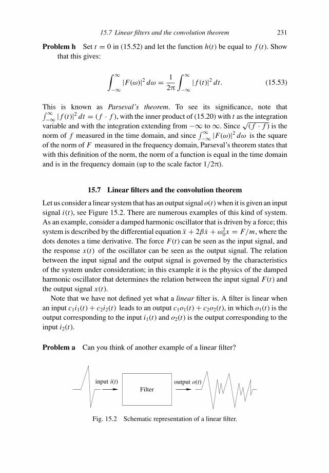
15.7 Linear filters and the convolution theorem 231
Problem h Set t = 0 in (15.52) and let the function h(t) be equal to f (t). Showthat this gives:
∫ ∞
−∞|F(ω)|2 dω = 1
2π
∫ ∞
−∞| f (t)|2 dt. (15.53)
This is known as Parseval’s theorem. To see its significance, note that∫ ∞−∞ | f (t)|2 dt = ( f · f ), with the inner product of (15.20) with t as the integrationvariable and with the integration extending from −∞ to ∞. Since
√( f · f ) is the
norm of f measured in the time domain, and since∫ ∞−∞ |F(ω)|2 dω is the square
of the norm of F measured in the frequency domain, Parseval’s theorem states thatwith this definition of the norm, the norm of a function is equal in the time domainand is in the frequency domain (up to the scale factor 1/2π).
15.7 Linear filters and the convolution theorem
Let us consider a linear system that has an output signal o(t) when it is given an inputsignal i(t), see Figure 15.2. There are numerous examples of this kind of system.As an example, consider a damped harmonic oscillator that is driven by a force; thissystem is described by the differential equation x + 2β x + ω2
0x = F/m, where thedots denotes a time derivative. The force F(t) can be seen as the input signal, andthe response x(t) of the oscillator can be seen as the output signal. The relationbetween the input signal and the output signal is governed by the characteristicsof the system under consideration; in this example it is the physics of the dampedharmonic oscillator that determines the relation between the input signal F(t) andthe output signal x(t).
Note that we have not defined yet what a linear filter is. A filter is linear whenan input c1i1(t) + c2i2(t) leads to an output c1o1(t) + c2o2(t), in which o1(t) is theoutput corresponding to the input i1(t) and o2(t) is the output corresponding to theinput i2(t).
Problem a Can you think of another example of a linear filter?
Filterinput i(t) output o(t)
Fig. 15.2 Schematic representation of a linear filter.
232 Fourier analysis
Problem b Can you think of a system that has one input signal and one outputsignal, in which these signals are related through a nonlinear relation? Thiswould be an example of a nonlinear filter; the theory of this section would notapply to such a filter.
It is possible to determine the output o(t) for any input i(t) if the output to adelta function input is known. Consider the special input signal δ(t − τ ) that con-sists of a delta function centered at t = τ . Since a delta function has “zero-width”(if it has a width at all) such an input function is impulsive. Let the output forthis particular input be denoted by g(t, τ ). Since this function is the responseat time t to an impulsive input at time τ this function is called the impulseresponse:
The impulse response function g(t, τ ) is the output of the system at timet due to an impulsive input at time τ .
How can the impulse response be used to find the response to an arbitrary inputfunction? Any input function can be written as:
i(t) =∫ ∞
−∞δ(t − τ )i(τ ) dτ . (15.54)
This identity follows from the definition of the delta function. However, we can alsolook at this expression from a different point of view. The integral on the right-handside of (15.54) can be seen as a superposition of infinitely many delta functionsδ(t − τ ). Each delta function when considered as a function of t is centered attime τ . Since we integrate over τ these different delta functions are superposed toconstruct the input signal i(t). Each of the delta functions in the integral (15.54) ismultiplied by i(τ ). This term plays the role of a coefficient that gives a weight tothe delta function δ(t − τ ).
At this point it is crucial to use that the filter is linear. Since the response to theinput δ(t − τ ) is the impulse response g(t, τ ), and since the input can be written asthe superposition (15.54) of delta function input signals δ(t − τ ), the output can bewritten as the same superposition of impulse response signals g(t, τ ):
o(t) =∫ ∞
−∞g(t, τ )i(τ ) dτ . (15.55)
Problem c Carefully compare (15.54) and (15.55). Note the similarity and makesure you understand the reasoning that has led to (15.55).

15.7 Linear filters and the convolution theorem 233
You may find this “derivation” of (15.55) rather vague. The notion of the impulseresponse will be treated in much greater detail in Chapter 18 because it plays acrucial role in mathematical physics.
At this point we make another assumption about the system. Apart from itslinearity we will also assume it is invariant for translations in time . This is acomplex way of saying that we assume that the properties of the filter do notchange with time. This is the case for the damped harmonic oscillator describedat the beginning of this section. However, this oscillator would not be invariantfor translations in time if the damping parameter were a function of time as well:β = β(t). In that case, the system would give different responses when the sameinput is used at different times.
When the properties of the filter do not depend on time, the impulse responseg(t, τ ) depends only on the difference t − τ . To see this, consider the dampedharmonic oscillator again. The response at a certain time depends only on the timethat has lapsed between the excitation at time τ and the time of observation t .Therefore, for a time-invariant filter:
g(t, τ ) = g(t − τ ). (15.56)
Inserting this in (15.55) shows that for a linear time-invariant filter the output isgiven by the convolution of the input with the impulse response:
o(t) =∫ ∞
−∞g(t − τ )i(τ ) dτ = (g ∗ i) (t). (15.57)
Problem d Let the Fourier transform of i(t) be given by I (ω), the Fourier trans-form of o(t) by O(ω) and the Fourier transform of g(t) by G(ω). Use (15.57)to show that these Fourier transforms are related by:
O(ω) = 2πG(ω)I (ω). (15.58)
Expressions (15.57) and (15.58) are key results in the theory in linear time-invariantfilters. The first of these states that one only needs to know the response g(t) to asingle impulse to compute the output of the filter to any input signal i(t). Equation(15.58) has two important consequences. First, if one knows the Fourier transformG(ω) of the impulse response, one can compute the Fourier transform O(ω) of theoutput. An inverse Fourier transform then gives the output o(t) in the time domain.
Problem e Show that for a fixed value of ω that G(ω)e−iωt is the response of thesystem to the input signal e−iωt .

234 Fourier analysis
This means that if one knows the response of the filter to the harmonic signal e−iωt
at any frequency, one knows G(ω) and the response to any input signal can bedetermined.
The second important consequence of (15.58) is that the output at frequencyω depends only on the input and impulse response at the same frequency ω, andnot on other frequencies. This last property does not hold for nonlinear systems,because for these different frequencies components of the input signal are mixedby the nonlinearity of the system. An example of this phenomenon is the Earth’sclimate which has variations which contain frequency components that cannot beexplained by periodic variations in the orbital parameters in the Earth, but whichare due to the nonlinear character of the climate response to the amount of energyreceived by the Sun [96].
The fact that a filter can be used either by specifying its Fourier transformG(ω) (or equivalently the response to an harmonic input e−iωt ) or by prescrib-ing the impulse response g(t) implies that a filter can be designed either in thefrequency domain or in the time domain. In Section 15.8 the action of a filterin the time domain is described. A Fourier transform then leads to a compactdescription of the filter response in the frequency domain. In Section 15.9 theconverse route is taken; the filter is designed in the frequency domain, and aFourier transform is used to derive an expression for the filter in the time do-main.
As a last reminder it should be mentioned that although the theory of linearfilters is introduced here for filters that act in the time domain, the theory is equallyvalid for filters in the spatial domain. In the latter case, the wavenumber k playsthe role that the angular frequency played in this section. Since there may be morethan one spatial dimension, the theory for the spatial domain must be generalizedto include higher-dimensional spatial Fourier transforms. However, this does notchange the principles involved. Examples can be found in Sections 21.2 and 21.3for the upward continuation of the Earth’s gravity field.
15.8 Dereverberation filter
As an example of a filter that is derived in the time domain we consider here thedescription of reverberations inmarine seismics. Suppose a seismic survey is carriedout at sea. In such an experiment a ship tows a string of hydrophones that record thepressure variations just below the surface of the water, see Figure 15.3. Since thepressure vanishes at the surface of the water, the surface of the water totally reflectspressure waves and the reflection coefficient for reflection at the water surface isequal to −1. Let the reflection coefficient for waves reflecting upwards from the

15.8 Dereverberation filter 235
r i(t − 2T)2
water
solid earth
i(t) −ri(t − T)
Fig. 15.3 The generation of reverberations in a marine seismic experiment.
sea bed be denoted by r . Since the contrast between the water and the solid earthbelow is not small, this reflection coefficient can be considerable. Because of energyconservation the reflected wave must be weaker than the incoming wave, so thatr ≤ 1.
Since the reflection coefficient of the sea bed is not small, waves can bounce backand forth repeatedly between thewater surface and the sea bed. These reverberationsare an unwanted artifact in seismic experiments. This is because a wave that hasbounced back and forth in the water layer can bemisinterpreted on a seismic sectionas a reflector in the Earth. For this reason onewants to eliminate these reverberationsfrom seismic data.
Suppose the wavefield recorded by the hydrophones in the absence of reverber-ations is denoted by i(t). Let the time it takes for a wave to travel from the watersurface to the sea bed and back be denoted by T ; this time is called the two-waytravel time.
Problem a Show that a wave that has bounced back and forth once is given by−ri(t − T ). Hint: determine the amplitude of this wave from the reflectioncoefficients it encounters on its path and account for the time delay due to thebouncing up and down once in the water layer.
Problem b Generalize this result to a wave that bounces back and forth n-timesin the water layer and show that the signal o(t) recorded by the hydrophonesis given by:
o(t) = i(t) − r i(t − T ) + r2 i(t − 2T ) + · · ·
236 Fourier analysis
or
o(t) =∞
∑
n=0
(−r )n i(t − nT ), (15.59)
see Figure 15.3.
The notation i(t) and o(t) that was introduced in the previous section is deliberatelyused here. The action of the reverberation in the water layer is seen as a linearfilter. The input of the filter i(t) is the wavefield that would have been recordedif the waves did not bounce back and forth in the water layer. The output is thewavefield that results from the reverberations in the water layer. In a marine seismicexperiment one records the wavefield o(t) while one would like to know the signali(t) that contains just the reflections from below the water bottom. The process ofremoving the reverberations from the signal is called “dereverberation.” The aimof this section is to derive a dereverberation filter that allows us to extract the inputi(t) from the recorded output o(t).
Problem c It may not be obvious that (15.59) describes a linear filter of the form(15.57) that maps the input i(t) onto the output o(t). Show that (15.59) can bewritten in the form (15.57) with the impulse response g(t) given by:
g(t) =∞
∑
n=0
(−r )n δ(t − nT ), (15.60)
with δ(t) the Dirac delta function.
Problem d Show that g(t) is indeed the impulse response. In other words, showthat if a delta function is incident as a primary arrival at the water surface thereverberations within the water layer lead to the signal (15.60).
The deconvolution can most simply be carried out in the frequency domain. Let theFourier transforms of i(t) and o(t), as defined by the transform (15.43), be denotedby I (ω) and O(ω) respectively. It follows from (15.59) that one needs to find theFourier transform of i(t − nT ).
Problem e According to the definition (15.43) the Fourier transform of i(t − τ )is given by (1/2π)
∫ ∞−∞ i(t − τ )eiωt dt . Use a change of the integration variable
to show that the Fourier transform of i(t − τ ) is given by I (ω)eiωτ .
What you have derived here is the shift property of the Fourier transform: atranslation of a function over a time τ corresponds in the frequency domain to

15.8 Dereverberation filter 237
a multiplication by eiωτ
i(t) ←→ I (ω),i(t − τ ) ←→ I (ω)eiωτ .
(15.61)
Problem f Apply a Fourier transform to (15.59) for the output, use the shift prop-erty (15.61) for each term and show that the output in the frequency domainis related to the Fourier transform of the input by the following expression:
O(ω) =∞
∑
n=0
(−r )n eiωnT I (ω). (15.62)
Problem g Use the theory of Section 15.7 to show that the filter that describesthe generation of reverberations is given in the frequency domain by:
G(ω) = 1
2π
∞∑
n=0
(−r )n eiωnT . (15.63)
Problem h Because of energy conservation, the reflection coefficient r is lessthan or equal to 1, therefore this series is guaranteed to converge. Sum thisseries to show that
G(ω) = 1
2π
1
1 + reiωT. (15.64)
This is a useful result because it implies that the output and the input in the frequencydomain are related by
O(ω) = 1
1 + reiωTI (ω). (15.65)
Note that the action of the reverberation leads in the frequency domain to a simpledivision by (1 + reiωT ). Note also that (15.65) has a form similar to (3.40) whichaccounts for the reverberation of waves between two stacks of reflectors. Thisresemblance is no coincidence because the physics of waves bouncing back andforth between two reflectors is similar.
Problem i The goal of this section was to derive a dereverberation filter thatproduces i(t) when o(t) is given. Use (15.65) to derive a dereverberation filterin the frequency domain.
The dereverberation filter you have just derived is simple in the frequency domain;it only involves a multiplication of every frequency component O(ω) by a scalar.
238 Fourier analysis
Since multiplication is a simple and efficient procedure it is attractive to carry outdereverberation in the frequency domain. The dereverberation filter you have justderived was developed originally by Backus [7].
The simplicity of the dereverberation filter hides a nasty complication. If thereflection coefficient r and the two-way travel time T are known exactly and if thesea bed is exactly horizontal there is no problem with the dereverberation filter.However, in practice one only has estimates of these quantities. Let these estimatesbe denoted by r ′ and T ′ respectively. The reverberations lead in the frequencydomain to a division by 1 + reiωT , while the dereverberation filter based on theestimated parameters leads to a multiplication with 1 + r ′eiωT ′
. The net effect ofthe generation of the reverberations and the subsequent dereverberation is thusgiven in the frequency domain by a multiplication by
1 + r ′eiωT ′
1 + reiωT.
Problem j Show that when the reflection coefficients are close to unity and whenthe estimate of the travel time is not accurate (T ′ = T ) the term given abovediffers appreciably from unity. Explain why this implies that the dereverbera-tion does not work well.
In practice one faces not only the problem that the estimates of the reflectioncoefficients and the two-way travel time may be inaccurate, but in addition the seabed may not be exactly flat and there may be variations in the reflection coefficientalong the sea bed. In which case the performance of the dereverberation filter canbe significantly degraded.
15.9 Design of frequency filters
In this section we consider the problem in which a time series i(t) is recorded andis contaminated with high-frequency noise. The aim of this section is to derive afilter in the time domain that removes the frequency components with a frequencygreater than a cut-off frequency ω0 from the time series. Such a filter is called alow-pass filter because only frequency components lower than the threshold ω0
pass the filter.
Problem a Show that this filter is given in the frequency domain by:
G(ω) =
1 if |ω| ≤ ω0
0 if |ω| > ω0. (15.66)
15.9 Design of frequency filters 239
Problem b Explain why the absolute value of the frequency should be used inthis expression.
Problem c Show that this filter is given in the time domain by
g(t) =∫ ω0
−ω0
e−iωt dω. (15.67)
Problem d Carry out the integration over frequency to derive that the filter isexplicitly given by
g(t) = 2ω0 sinc (ω0t) , (15.68)
where the sinc function is defined by
sinc x ≡ sin x
x. (15.69)
Problem e Sketch the impulse response (15.68) of the low-pass filter as a functionof time. Determine the behavior of the filter for t = 0 and show that the firstzero-crossing of the filter is at time t = ±π/ω0.
The zero-crossing of the filter is of fundamental importance. It implies that thewidth of the impulse response in the time domain is given by 2π/ω0.
Problem f Use expression (15.66) to show that the width of the filter in thefrequency domain is given by 2ω0.
This means that when the the cut-off frequency ω0 is increased, the width of thefilter in the frequency domain increases but the width of the filter in the time domaindecreases. A large width of the filter in the frequency domain corresponds to a smallwidth of the filter in the time domain and vice versa.
Problem g Show that the product of the width of the filter in the time domain andthe width of the same filter in the frequency domain is given by 4π.
The significance of this result is that this product is independent of the frequencyω0. This implies that the filter cannot be arbitrarily peaked in both the time domainand the frequency domain. This effect has pronounced consequences since it is theessence of the uncertainty relation of Heisenberg which states that the position andmomentum of a particle can never be known exactly; more details can be found inthe book of Merzbacher [69].
240 Fourier analysis
The filter (15.68) does not actually have very desirable properties; it has twobasic problems. The first problem is that the filter decays slowly with time. Thismeans that the length of the filter in the time domain is very great, and hence theconvolution of a time series with the filter is numerically a rather inefficient process.This can be solved by making the cut-off of the filter in the frequency domain moregradual than the frequency cut-off defined in (15.66), for example by using the filterG(ω) = (1 + |ω| /ω0)−n with n a positive integer.
Problem h Does this filter have the steepest cut-off for low values of n or for highvalues of n? Hint: make a plot of G(ω) as a function of ω.
The second problem is that the filter is not causal. This means that when a functionis convolved with the filter (15.68), the output of the filter depends on the valueof the input at later times, that is the filter output depends on the input in thefuture.
Problem i Show that this is the case, and that the output depends on the input ofearlier times only when g(t) = 0 for t < 0.
A causal filter can be designed by using the theory of analytic functions describedin Chapter 16. The design of filters is quite an art; details can be found for examplein the books of Robinson and Treitel [90] or Claerbout [27].
15.10 Linear filters and linear algebra
There is a close analogy between the theory of linear filters of Section 15.7 and theeigenvector decomposition of a matrix in linear algebra as treated in Section 13.4.To see this we will use the same notation as in Section 15.7 and use the Fouriertransform (15.45) to write the output of the filter in the time domain as:
o(t) =∫ ∞
−∞O(ω)e−iωt dω. (15.70)
Problem a Use expression (15.58) to show that this can be written as
o(t) = 2π∫ ∞
−∞G(ω)I (ω)e−iωt dω, (15.71)
15.10 Linear filters and linear algebra 241
and carry out an inverse Fourier transformation of I (ω) to derive that
o(t) =∞
∫∫
−∞G(ω)e−iωt eiωτ i(τ ) dωdτ . (15.72)
In order to establish the connection with linear algebra we introduce by analogywith (15.33) the following basis functions:
uω(t) ≡ 1√2π
e−iωt , (15.73)
and the inner product
( f · g) ≡∫ ∞
−∞f ∗(t)g(t) dt. (15.74)
Problem b Use the results of Section 15.4 to show that these basis functions areorthonormal for this inner product in the sense that
(
uω · uω′) = δ(ω − ω′). (15.75)
Problem c These functions play the same role as the eigenvectors in Sec-tion 13.4. To which expression in Section 13.4 does the above expressioncorrespond?
Problem d Show that (15.72) can be written as
o(t) =∫ ∞
−∞G(ω)uω(t) (uω · i) dω. (15.76)
This expression should be compared with
Ap =N
∑
n=1
λn v(n)(
v(n) · p)
. (13.44)
The integration over frequency plays the same role as the summation over eigen-vectors in (13.44). Expression (15.76) can be seen as a description for the operatorg(t) in the time domain that maps the input function i(t) onto the output o(t).
Problem e Use (15.57), (15.74), and (15.76) to show that:
g(t − τ ) = 2π∫ ∞
−∞G(ω)uω(t)u
∗ω(τ ) dω. (15.77)
242 Fourier analysis
There is a close analogy between this expression and the dyadic decompo-sition of a matrix into its eigenvectors and eigenvalues derived in Section13.4.
Problem f To see this connection show that (13.45) can be written in componentform as:
Ai j =N
∑
n=1
λn v(n)i v
(n)Tj . (15.78)
The sum over eigenvalues in (15.78) corresponds to the integration over frequencyin (15.77). In Section 13.4 linear algebra in a finite-dimensional vector space wastreated. In such a space there is a finite number of eigenvalues. In this section, afunction space with infinitely many degrees of freedom is analyzed; it will comeas no surprise that for this reason the sum over a finite number of eigenvaluesshould be replaced by an integration over the continuous variable ω. The index iin (15.78) corresponds to the variable t in (15.77) while the index j corresponds tothe variable τ .
Problem g Establish the connection between all variables in (15.77) and (15.78).Show specifically that G(ω) plays the role of eigenvalue λn and uω plays therole of eigenvector. Which operation in (15.77) corresponds to the transposethat is taken of the second eigenvector in (15.78)?
You may wonder why the function uω(t) = e−iωt/√2π, defined in (15.73), and
not some other function plays the role of the eigenvector of the impulse responseoperator g(t − τ ). To see why this is so we have to understand what a linear filteractually does. Let us first consider the example of the reverberation filter of Section15.8. According to (15.59) the reverberation filter is given by:
o(t) = i(t) − ri(t − T ) + r2i(t − 2T ) + · · · . (15.59)
It follows from this expression that what the filter really does is to take the in-put i(t), translate it over a time nT to a new function i(t − nT ), multiply eachterm with (−r )n and sum over all values of n. This means that the filter is a com-bination of three operations: (i) translation in time, (ii) multiplication, and (iii)summation over n. The same conclusion holds for any general time-invariant linearfilter.
15.10 Linear filters and linear algebra 243
Problem h Use a change of the integration variable to show that the action of atime-invariant linear filter as given in (15.57) can be written as
o(t) =∫ ∞
−∞g(τ )i(t − τ ) dτ . (15.79)
The function i(t − τ ) is the function i(t) translated over a time τ . This translatedfunction is multiplied by g(τ ) and an integration over all values of τ is carried out.This means that in general the action of a linear filter can be seen as a combinationof translation in time, multiplication, and integration over all translations τ . Howcan this be used to explain that the correct eigenfunctions to be used are uω(t) =e−iωt/
√2π? The answer does not lie in the multiplication because any function is
an eigenfunction of the operator that carries out multplication by a constant, that isa f (t) = λ f (t) for every function f (t) with the eigenvalue λ = a. This means thatthe translation operator is the reason that the eigenfunctions areuω(t) = e−iωt/
√2π.
Let the operator that carries out a translation over a time τ be denoted by Tτ :
Tτ f (t) ≡ f (t − τ ). (15.80)
Problem i Show that the functions uω(t) defined in (15.73) are the eigenfunctionsof the translation operator Tτ , that is show that Tτ uω(t) = λuω(t). Express theeigenvalue λ of the translation operator in terms of the translation time τ .
Problem j Compare this result with the shift property of the Fourier transformthat was derived in (15.61).
This means that the functions uω(t) are the eigenfunctions to be used for the eigen-function decomposition of a linear time-invariant filter, because these functions areeigenfunctions of the translation operator.
Problem k You identified in problem e the eigenvalues of the filter with G(ω).Show that this interpretation is correct: in other words show that when thefilter g acts on the function uω(t) the result can be written as G(ω)uω(t). Hint:go back to problem e of Section 15.7.
This analysis shows that the Fourier transform, which uses the functions e−iωt , isso useful because these functions are the eigenfunctions of the translation operator.However, this also points to a limitation of the Fourier transform. Consider a linearfilter that is not time-invariant, that is afilter inwhich the output does not dependonly
244 Fourier analysis
on the difference between the input time τ and the output time t . Such a filter satisfiesthe general equation (15.55) rather than the convolution integral (15.57). The actionof a filter that is not time-invariant cannot in general be written as a combination ofthe following operations: multiplication, translation, and integration. This meansthat for such a filter the functions e−iωt that form the basis of the Fourier transformare not the appropriate eigenfunctions. The upshot of this is that in practice theFourier transform is only useful for systems that are time-invariant, or in generalthat are translationally invariant in the coordinate that is used.

16
Analytic functions
In this chapter we consider complex functions in the complex plane. The reason fordoing this is that the requirement that the function “behaves well” (this is definedlater) imposes remarkable constraints on such complex functions. Since these con-straints coincide with some of the laws of physics, the theory of complex functionshas a number of important applications in mathematical physics. In this chaptercomplex functions h(z) are treated that are decomposed into real and imaginaryparts:
h(z) = f (z) + ig(z); (16.1)
hence the functions f (z) and g(z) are assumed to be real. The complex number z iswritten as z = x + iy, so that x = e(z) and y = m(z), where e and m denotethe real and imaginary part respectively.
16.1 Theorem of Cauchy–Riemann
Let us first consider a real function F(x) of a real variable x . The derivative of sucha function is defined by the rule
d F
dx= lim
x→0
F(x + x) − F(x)
x. (16.2)
In general there are two ways in which x can approach zero: from above andfrom below. For a function that is differentiable it does not matter whether xapproaches zero from above or from below. If the limits x ↓ 0 and x ↑ 0 dogive a different result it is a sign that the function does not behave well, it has akink and the derivative is not unambiguously defined, see Figure 16.1.
245

246 Analytic functions
∆x > 0∆x < 0
x
F(x)
Fig. 16.1 A function F(x) that is not differentiable.
Fig. 16.2 Examples of paths along which the limit z → 0 can be taken.
For complex functions the derivative is defined in the same way as in (16.1) forreal functions:
dh
dz= lim
z→0
h(z + z) − h(z)
z. (16.3)
For real functions, x could approach zero in two ways: from below and fromabove. However, the limit z → 0 in (16.3) can be taken in infinitely many ways.As an example see Figure 16.2 where some different paths that one can use to letz approach zero are sketched. These do not necessarily give the same result.
Problem a Consider the function h(z) = e1/z . Using the definition (16.3) computedh/dz at the point z = 0 when z approaches zero: (i) from the positive realaxis, (ii) from the negative real axis, (iii) from the positive imaginary axis, and(iv) from the negative imaginary axis.
16.1 Theorem of Cauchy–Riemann 247
You have discovered that for some functions the result of the limit z dependscritically on the path that one uses in the limit process. The derivative of such afunction is not defined unambiguously. However, for many functions the value ofthe derivative does not depend on the way that z approaches zero. When thesefunctions and their derivatives are also finite, they are called analytic functions. Therequirement that the derivative does not depend on the way in which z approacheszero imposes a constraint on the real and imaginary parts of the complex function.To see this we will let z approach zero along the real axis and along the imaginaryaxis.
Problem b Consider a complex function of the form (16.1) and compute thederivative dh/dz by setting z = x with x a real number. (Hence zapproaches zero along the real axis.) Show that the derivative is given bydh/dz = ∂ f/∂x + i∂g/∂x .
Problem c Compute the derivative dh/dz also by setting z = iy with y areal number. (Hence z approaches zero along the imaginary axis.) Show thatthe derivative is given by dh/dz = ∂g/∂y − i∂ f/∂y.
Problem d When h(z) is analytic these two expressions for the derivative are bydefinition equal. Show that this implies that:
∂ f
∂x= ∂g
∂y, (16.4)
∂g
∂x= −∂ f
∂y. (16.5)
These are puzzling expressions since (16.4) and (16.5) imply that the realand imaginary parts of an analytic complex function are not independent ofeach other: they are coupled by the constraints imposed by equations (16.4)and (16.5). Expressions (16.4) and (16.5) are called the Cauchy–Riemannrelations.
Problem e Use these relations to show that both f (x, y) and g(x, y) are harmonicfunctions. These are functions for which the Laplacian vanishes:
∇2 f = ∇2g = 0. (16.6)
Hence we have found not only that f and g are coupled to each other; in additionthe functions f and g must be harmonic functions. This is exactly the reason whythis theory is so useful in mathematical physics because harmonic functions arise

248 Analytic functions
in several applications, see the examples in the coming sections. However, we havenot found all the properties of harmonic functions yet.
Problem f Show that:
(∇ f · ∇g) = 0. (16.7)
Since the gradient of a function is perpendicular to the lines where the functionis constant this implies that the curves where f is constant and where g is constantintersect each other at a fixed angle.
Problem g Determine this angle.
Problem h Verify the properties (16.4)–(16.7) explicitly for the function h(z) =z2. Also sketch the lines in the complex plane where f = e(h) and g =m(h) are constant.
We have still not fully explored all the properties of analytic functions. Let usconsider a line integral
∮
C h(z)dz along a closed contour C in the complex plane.
Problem i Use the property dz = dx + idy to deduce that:∮
Ch(z)dz =
∮
Cv · dr + i
∮
Cw · dr, (16.8)
where dr =(
dxdy
)
and the vectors v and w are defined by:
v =(
f−g
)
, w =(
gf
)
. (16.9)
Note that we are now using x and y in a dual role as the real and imaginary parts ofa complex number, as well as the Cartesian coordinates in a plane. In the followingproblem we will (perhaps confusingly) use the notation z both for a complex numberin the complex plane, as well as for the familiar z-coordinate in a three-dimensionalCartesian coordinate system.
Problem j Show that the Cauchy–Riemann relations (16.4)–(16.5) imply that thez-component of the curl of v and w vanishes: (∇ × v)z = (∇ × w)z = 0, anduse (16.8) and the theorem of Stokes (9.2) to show that when h(z) is analytic
16.2 Electric potential 249
everywhere within the contour C :∮
Ch(z) dz = 0, where h(z) is analytic within C. (16.10)
This means that the line integral of a complex functions along any contour whichencloses a region of the complex plane where that function is analytic is equal tozero. We will make extensive use of this property in Chapter 17 where we treatintegration in the complex plane.
16.2 Electric potential
Analytic functions are often useful in the determination of the electric field andthe potential for two-dimensional problems. The electric field satisfies the fieldequation (8.13): (∇ · E) = ρ(r)/ε0. In free space the charge-density vanishes, hence(∇ · E) = 0. The electric field is related to the potential V through the relation
E = −∇V . (16.11)
Problem a Show that in free space the potential is a harmonic function:
∇2V (x, y) = 0. (16.12)
We can exploit the theory of analytic functions by noting that the real and imaginaryparts of analytic functions both satisfy (16.12). This implies that if we take V (x, y)to be the real part of a complex analytic function h(x + iy), (16.12) is automaticallysatisfied.
Problem b It follows from (16.11) that the electric field is perpendicular to thelines where V is constant. Show that this implies that the electric field linesare also perpendicular to the lines V = const . Use the theory of the previoussection to argue that the field lines are the lines where the imaginary part ofh(x + iy) is constant.
This means that we receive a bonus by expressing the potential V as the real partof a complex analytic function, because the field lines simply follow from therequirement that m(h) = const.
Suppose we want to know the potential in the half-space y ≥ 0 when we havespecified the potential on the x-axis. (Mathematically this means that we want tosolve the equation ∇2V = 0 for y ≥ 0 when V (x, y = 0) is given.) If we can findan analytic function h(x + iy) such that on the x-axis (where y = 0) the real part

250 Analytic functions
of h is equal to the potential, we have solved our problem because the real part ofh by definition satisfies the required boundary condition and it satisfies the fieldequation (16.12).
Problem c Consider a potential that is given on the x-axis by
V (x, y = 0) = V0 e−x2/a2. (16.13)
Show that on the x-axis this function can be written as V = e(h) with
h(z) = V0 e−z2/a2. (16.14)
Problem d This means that we can determine the potential and the field linesthroughout the half-plane y ≥ 0. Use the theory of this section to show thatthe potential is given by
V (x, y) = V0 e(y2−x2)/a2cos
(
2xy
a2
)
. (16.15)
Problem e Verify explicitly that this solution satisfies the boundary condition atthe x-axis and that it satisfies the field equation (16.12).
Problem f Show that the field lines are given by the relation
e(y2−x2)/a2sin
(
2xy
a2
)
= const. (16.16)
Problem g Sketch the field lines and the lines where the potential is constant inthe half-space y ≥ 0.
In this derivation we have extended the solution V (x, y) into the upper half-plane by identifying it with an analytic function in the half-plane which has on thex-axis a real part which equals the potential on the x-axis. Note that we found thesolution to this problem without explicitly solving the partial differential equation(16.12) which governs the potential. The approach we have taken is called analyticcontinuation since we continue an analytic function from one region (the x-axis)into the upper half-plane. Analytic continuation turns out to be a very unstableprocess. This can be verified explicitly for this example.
Problem h Sketch the potential V (x, y) as a function of x for the values y = 0,y = a, and y = 10a. What is the wavelength of the oscillations in the x-direction of the potential V (x, y) for these values of y? Show that when weslightly perturb the constant a the perturbation of the potential increases forincreasing values of y. This implies that when we slightly perturb the boundary
16.3 Fluid flow and analytic functions 251
condition the solution is more perturbed as we move further away from thatboundary.
16.3 Fluid flow and analytic functions
As a second application of the theory of analytic functions we consider fluid flow. Atthe end of Section 6.2 we saw that the streamlines of the flow can be determined bysolving the differential equations dr/dt = v(r) for the velocity field (6.16)–(6.17).This requires the solution of a system of nonlinear differential equations which isvery difficult. Here the theory of analytic functions is used to solve this problem ina simple way. We consider once again a fluid that is incompressible ((∇ · v) = 0)and specialize to the special case in which the vorticity of the flow vanishes:
∇ × v = 0. (16.17)
Such a flow is called irrotational because it does not rotate (see Sections 7.3 and7.4). The requirement (16.17) is automatically satisfied when the velocity is thegradient of a scalar function f :
v = ∇ f. (16.18)
Problem a Show this by taking the curl of the previous expression.
The function f plays the same role for the velocity field v as the electric potentialV does for the electric field E. For this reason, flow with a vorticity equal to zerois called potential flow.
Problem b Show that the requirement that the flow is incompressible implies that
∇2 f = 0. (16.19)
We now specialize to the special case of incompressible and irrotational flow intwo dimensions. In that case we can again use the theory of analytic functions todescribe the flow field. Once we can identify the potential f (x, y) with the real partof an analytic function h(x + iy) we know that (16.19) must be satisfied.
Problem c Consider the velocity field (6.13) due to a point source at r = 0. Showthat this flow field follows from the potential
f (x, y) = V
2πln r, (16.20)
where r =√
x2 + y2.

252 Analytic functions
Problem d Verify explicitly that this potential satisfies (16.19) except for r = 0.For what physical reason is (16.19) not satisfied at r = 0?
We now want to identify the potential f (x, y) with the real part of an analytic func-tion h(x + iy). We know already that the flow follows from the requirement that thevelocity is the gradient of the potential, hence it follows by taking the gradient of thereal part of h. The curves f = const. are perpendicular to the flow because v = ∇ fis perpendicular to these curves. However, it was shown in Section 16.1 that thecurves g = m(h) = const. are perpendicular to the curves f = e(h) = const.This means that the flow lines are given by the curves g = m(h) = const. Inorder to use this, we first have to find an analytic function with a real part given by(16.20). The simplest guess is to replace r in (16.20) by the complex variable z:
h(z) = V
2πln z. (16.21)
Problem e Verify that for complex z the real part of this function indeed satisfies(16.20) and that the imaginary part g of this function is given by:
g = V
2πϕ, (16.22)
where ϕ = arctan (y/x) is the argument of the complex number. Hint: use therepresentation z = reiϕ for the complex numbers.
Problem f Sketch the lines g(x, y) = const. and verify that these lines indeedrepresent the flow lines in this flow.
Now we consider the more complicated problem in Section 6.2 in which the flowhas a source at r+ = (L , 0) and a sink at r− = (−L , 0). The velocity field is givenby (6.16) and (6.17) and our goal is to determine the flow lines without solving thedifferential equation dr/dt = v(r). The points r+ and r− can be represented in thecomplex plane by the complex numbers z+ = L + i0 and z− = −L + i0 respec-tively. For the source at r+ flow is represented by the potential (V /2π) ln |z − z+|;this follows from the solution (16.21) for a single source by moving this source toz = z+.
Problem g Using a similar reasoning determine the contribution to the potentialf by the sink at r−. Show that the potential of the total flow is given by:
f (z) = V
2πln
( |z − z+||z − z−|
)
. (16.23)

16.3 Fluid flow and analytic functions 253
z+
−r +r
−z
− +
z
Fig. 16.3 Definition of the geometric variables for the fluid flow with a sourceand a sink.
Problem h Express this potential in x and y, compute the gradient, and verifythat this potential indeed gives the flow of (6.16)–(6.17). You may find Figure16.3 helpful.
We have found that the potential f is the real part of the complex function
h(z) = V
2πln
(
z − z+z − z−
)
. (16.24)
Problem i Write z − z± = r±eiϕ± (with r± and ϕ± defined in Figure 16.3), takethe imaginary part of (16.24), and show that g = m(h) is given by:
g = V
2π
(
ϕ+ − ϕ−)
. (16.25)
Problem j Show that the streamlines of the flow are given by the relation
arctan
(
y
x − L
)
− arctan
(
y
x + L
)
= const. (16.26)
A plot of the streamlines can thus be drawn by making a contour plot of thefunction on the left-hand side of (16.26). This treatment is simpler than solving thedifferential equation dr/dt = v(r).

17
Complex integration
In Chapter 16 the properties of analytic functions in the complex plane were treated.One of the key results is that the contour integral of a complex function is equalto zero when the function is analytic everywhere in the area of the complex planeenclosed by that contour, see (16.10). From this it follows that the integral of acomplex function along a closed contour is nonzero only when the function is notanalytic in the area enclosed by the contour. Functions that are not analytic comein different types. In this section complex functions are considered that are notanalytic only at isolated points. These points where the function is not analytic arecalled the poles of the function.
17.1 Nonanalytic functions
When a complex function is analytic at a point z0, it can be expanded in a Taylorseries around that point. This implies that within a certain region around z0 thefunction can be written as:
h(z) =∞
∑
n=0
an(z − z0)n. (17.1)
Note that in this sum only positive powers of (z − z0) appear.
Problem a Show that the function h(z) = sin(z)/z can be written as a Taylor seriesaround the point z0 = 0 of the form (17.1) and determine the coefficients an .
Not all functions can be represented in a series of the form (17.1). As an exampleconsider the function h(z) = e1/z . The function is not analytic at the point z = 0
254
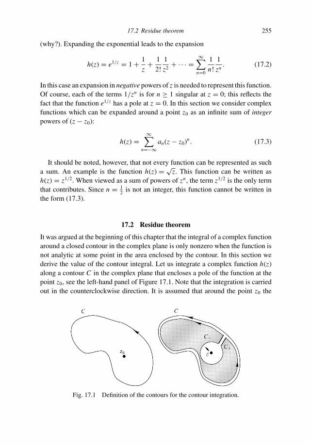
17.2 Residue theorem 255
(why?). Expanding the exponential leads to the expansion
h(z) = e1/z = 1 + 1
z+ 1
2!
1
z2+ · · · =
∞∑
n=0
1
n!
1
zn. (17.2)
In this case an expansion in negative powers of z is needed to represent this function.Of course, each of the terms 1/zn is for n ≥ 1 singular at z = 0; this reflects thefact that the function e1/z has a pole at z = 0. In this section we consider complexfunctions which can be expanded around a point z0 as an infinite sum of integerpowers of (z − z0):
h(z) =∞
∑
n=−∞an(z − z0)n. (17.3)
It should be noted, however, that not every function can be represented as sucha sum. An example is the function h(z) = √
z. This function can be written ash(z) = z1/2. When viewed as a sum of powers of zn , the term z1/2 is the only termthat contributes. Since n = 1
2 is not an integer, this function cannot be written inthe form (17.3).
17.2 Residue theorem
It was argued at the beginning of this chapter that the integral of a complex functionaround a closed contour in the complex plane is only nonzero when the function isnot analytic at some point in the area enclosed by the contour. In this section wederive the value of the contour integral. Let us integrate a complex function h(z)along a contour C in the complex plane that encloses a pole of the function at thepoint z0, see the left-hand panel of Figure 17.1. Note that the integration is carriedout in the counterclockwise direction. It is assumed that around the point z0 the
Fig. 17.1 Definition of the contours for the contour integration.

256 Complex integration
function h(z) can be expanded in a power series of the form (17.3). It is our goal todetermine the value of the contour integral
∮
C h(z)dz.The first step in the determination of the contour integral is to recognize that
within the shaded area in the right-hand panel of Figure 17.1 the function h(z) isanalytic because we have assumed that h(z) is only nonanalytic at the point z0. Byvirtue of the identity (16.10) this implies that
∮
C∗h(z) dz = 0, (17.4)
where the path C∗ consists of the contour C , a small circle with radius ε around z0
and the paths C+ and C− in the right-hand panel of Figure 17.1.
Problem a Show that the integrals along C+ and C− do not give a net contributionto the total integral:
∫
C+h(z) dz +
∫
C−h(z) dz = 0. (17.5)
Hint: note the opposite directions of integration along the paths C+ and C−.
Problem b Use this result and (17.4) to show that the integral along the originalcontour C is identical to the integral along the small circle Cε around the pointwhere h(z) is not analytic:
∮
Ch(z) dz =
∮
Cε
h(z) dz. (17.6)
Problem c The integration along C is in the counterclockwise direction. Is theintegration along Cε in the clockwise or in the counter-clockwise direction?
Expression (17.6) is useful because the integral along the small circle can be eval-uated by using that close to z0 the function h(z) can be written as the series (17.3).When one does this the integration path Cε needs to be parameterized. This can beachieved by writing the points on the path Cε as
z = z0 + εeiϕ , (17.7)
with ϕ running from 0 to 2π since Cε is a complete circle.
Problem d Use (17.3), (17.6), and (17.7) to derive that∮
Ch(z) dz =
∞∑
n=−∞ianε
(n+1)∫ 2π
0ei(n+1)ϕdϕ. (17.8)
17.2 Residue theorem 257
This is useful because it expresses the contour integral in the coefficients an ofthe expansion (17.3). It turns out that only the coefficient a−1 gives a nonzerocontribution.
Problem e Show by direct integration that:∫ 2π
0eimϕdϕ =
0 for m = 02π for m = 0
. (17.9)
Problem f Use this result to derive that only the term n = −1 contributes to thesum on the right-hand side of (17.8) and that
∮
Ch(z) dz = 2πia−1 (17.10)
It may seem surprising that only the term n = −1 contributes to the sum on theright-hand side of (17.8). However, we could have anticipated this result becausewe had already discovered that the contour integral does not depend on the precisechoice of the integration path. It can be seen that in the sum (17.8) each term isproportional to ε(n+1). Since we know that the integral does not depend on the choiceof the integration path, and hence on the size of the circle Cε, one would expect thatonly terms which do not depend on the radius ε contribute. This is only the casewhen n + 1 = 0, hence only for the term n = −1 is the contribution independentof the size of the circle. It is indeed only this term that gives a nonzero contributionto the contour integral.
The coefficient a−1 is usually called the residue and is denoted by the symbolRes h(z0) rather than a−1. However, remember that there is nothing mysteriousabout the residue, it is simply defined as
Res h(z0) ≡ a−1. (17.11)
With this definition the result (17.10) can trivially be written as∮
Ch(z) dz = 2πiRes h(z0) (counterclockwise direction). (17.12)
This may appear to be a rather uninformative rewrite of (17.10) but it is the form(17.12) that you will find in the literature. The identity (17.12) is called the residuetheorem.
Of course the residue theorem is only useful when one can determine the co-efficient a−1 in the expansion (17.3). You can find in Section 2.12 of Butkov [24]an overview of methods for computing the residue. Here we present the two most

258 Complex integration
widely used ones. The first method is to determine the power series expansion(17.3) of the function explicitly.
Problem g Determine the power series expansion of the function h(z) = sin(z)/z4
around z = 0 and use this expansion to find the residue.
Unfortunately, this method does not always work. For some special functions othertricks can be used. Here we consider functions with a simple pole; these are functionswhere the terms for n < −1 do not contribute in the expansion (17.3):
h(z) =∞
∑
n=−1
an(z − z0)n. (17.13)
An example of such a function is h(z) = cos(z)/z. The residue at the point z0
follows by “extracting” the coefficient a−1 from (17.13).
Problem h Multiply (17.13) by (z − z0), and take the limit z → z0 to show that:
Res h(z0) = limz→z0
(z − z0)h(z) (simple pole). (17.14)
However, remember that this recipe works only for functions with a simple pole,it gives the wrong answer (infinity) when applied to a function which has nonzerocoefficients an for n < −1 in (17.3).
In the treatment in this section we have considered an integration in the coun-terclockwise direction around the pole z0.
Problem i Repeat the derivation of this section for a contour integration in theclockwise direction around the pole z0 and show that in that case
∮
Ch(z) dz = −2πiRes h(z0) (clockwise direction). (17.15)
Find out in which step of the derivation the minus sign is picked up!
Problem j It may happen that a contour encloses not a single pole but a numberof poles at points z j . Find for this case a contour similar to the contour C∗ inthe right-hand panel of Figure 17.1 to show that the contour integral is equalto the sum of the contour integrals around the individual poles z j . Use this toshow that for this situation:
∮
Ch(z) dz = 2πi
∑
j
Res h(z j ) (counterclockwise direction). (17.16)

17.3 Solving integrals without knowing the primitive function 259
17.3 Solving integrals without knowing the primitive function
The residue theorem has some applications to integrals that do not contain a complexvariable at all! As an example consider the integral
I =∫ ∞
−∞
1
1 + x2dx . (17.17)
If you know that 1/(1 + x2) is the derivative of arctan x it is not difficult to solvethis integral:
I = [arctan x]∞−∞ = π
2−
(
−π
2
)
= π. (17.18)
Now suppose you did not know that arctan x is the primitive function of 1/(1 + x2).In that case you would be unable to see that the integral (17.17) is equal to π.Complex integration offers a way to obtain the value of this integral in a systematicfashion.
First note that the path of integration in the integral can be viewed as the realaxis in the complex plane. Nothing prevents us from viewing the real function1/(1 + x2) as a complex function 1/(1 + z2) because on the real axis z is equal tox . This means that
I =∫
Creal
1
1 + z2dz, (17.19)
where Creal denotes the real axis as integration path. At this point we cannot yetapply the residue theorem because the integration is not over a closed contour in thecomplex plane, see Figure 17.2. Let us close the integration path using the circular
x
x
R
z = i
z = −i
C
CR
real
Fig. 17.2 Definition of the integration paths in the complex plane.
260 Complex integration
path CR in the upper half-plane with radius R, see Figure 17.2. At the end of thecalculation we will let R go to infinity so that the integration over the semicirclemoves to infinity.
Problem a Show that
I =∫
Creal
1
1 + z2dz =
∮
C
1
1 + z2dz −
∫
CR
1
1 + z2dz. (17.20)
The circular integral is over the closed contour in Figure 17.2. What we have doneis close the contour and subtract the integral over the semicircle that we added toobtain a closed integration path. This is the general approach in the application ofthe residue theorem; one adds segments to the integration path to obtain an integralover a closed contour in the complex plane, and corrects for the segments that onehas added to the path. Obviously, this is only useful when the integral over thesegment that one has added can be computed easily or when it vanishes. In thisexample the integral over the semicircle vanishes as R → ∞. This can be seenfrom the following estimations:
∣
∣
∣
∣
∫
CR
1
1 + z2dz
∣
∣
∣
∣
≤∫
CR
∣
∣
∣
∣
1
1 + z2
∣
∣
∣
∣
|dz| ≤∫
CR
1
|z|2 − 1|dz| = πR
R2 − 1→ 0
as R → ∞. (17.21)
The estimate (17.21) implies that the last integral in (17.20) vanishes in the limitR → ∞. This means that
I =∮
C
1
1 + z2dz. (17.22)
Now we are in the position to apply the residue theorem because we have reducedthe problem to the evaluation of an integral along a closed contour in the complexplane. We know from Section 17.2 that this integral is determined by the poles ofthe function that is integrated within the contour.
Problem b Show that the function 1/(1 + z2) has poles for z = +i and z = −i .
Only the pole at z = +i is within contour C , see Figure 17.2. Since 1/(1 + z2) =1/[(z − i)(z + i)] this pole is simple (why?).
Problem c Use (17.14) to show that for the pole at z = i the residue is given by:Res = 1/2i .
17.3 Solving integrals without knowing the primitive function 261
Problem d Use the residue theorem (17.12) to deduce that
I =∫ ∞
−∞
1
1 + x2dx = π. (17.23)
This value is identical to the value obtained at the beginning of this section byusing that the primitive of 1/(1 + x2) is equal to arctan x . Note that the analysis issystematic and that we did not need to “know” the primitive function.
In the treatment of this problem there is no reason why the contour shouldbe closed in the upper half-plane. The estimate (17.21) holds equally well for asemicircle in the lower half-plane.
Problem e Repeat the analysis of this section with the contour closed in the lowerhalf-plane. Use that now the pole at z = −i contributes and take into accountthat the sense of integration is in the clockwise rather than the anticlockwisedirection. Show that this leads to the same result (17.23) that was obtained byclosing the contour in the upper half-plane.
In the evaluation of the integral (17.17) there was freedom whether to close thecontour in the upper half-plane or in the lower half-plane. This is not always thecase. To see this consider the integral
J =∫ ∞
−∞
cos (x − π/4)
1 + x2dx . (17.24)
Since eix = cos x + i sin x this integral can be written as
J = e
(∫ ∞
−∞
ei(x−π/4)
1 + x2dx
)
, (17.25)
where e(· · ·) again denotes the real part. We want to evaluate this integral byclosing this integration path with a semicircle either in the upper half-plane or inthe lower half-plane. Due to the term eix in the integral we now have no real choice inthis issue. The decision whether to close the integral in the upper half-plane or in thelower half-plane is dictated by the requirement that the integral over the semicirclevanishes as R → ∞. This can only happen when the integrand vanishes (fasterthan 1/R) as R → ∞. Let z be a point in the complex plane on the semicircle CR
that we use for closing the contour. On the semicircle z can be written as z = Reiϕ ,where in the upper half-plane 0 ≤ ϕ < π and in the lower half-plane π ≤ ϕ < 2π.
Problem f Use this representation of z to show that∣
∣eiz∣
∣ = e−R sin ϕ. (17.26)
262 Complex integration
Problem g Show that in the limit R → ∞ this term only goes to zero when z isin the upper half-plane.
This means that the integral over the semicircle only vanishes when we close thecontour in the upper half-plane. Using steps similar to those in (17.21) one can showthat the integral over a semicircle in the upper half-plane vanishes as R → ∞.
Problem h Take exactly the same steps as in the derivation of (17.23) and showthat
∫ ∞
−∞
cos (x − π/4)
1 + x2dx = π√
2 e. (17.27)
Note that this integral is equal to a combination of the three irrational numbersπ,
√2, and e!
Problem i Determine the integral∫ ∞−∞[sin(x − π/4)/(1 + x2)]dx without do-
ing any additional calculations. Hint: look carefully at (17.25) and spotsin (x − π/4).
It is important to note that in finding the integrals in this section we did notneed to know the primitive function of the function that we integrated. This isthe reason why complex integration is such a powerful technique; it allows us tosolve many integrals without knowing their primitive functions. The structure of thesingularities of the integrand in the complex plane and the behavior of the functionon a bounding contour carry sufficient information to integrate the function. Thisrather miraculous property is due to the fact that according to (16.6) in regionswhere the integrand is analytic it satisfies Laplace’s equation: ∇2 f = ∇2g = 0(where f and g are the real and imaginary parts of the integrand respectively).The singularities of the integrand act as sources or sinks for f and g. We havelearned already that the specification of the sources and sinks (ρ) plus boundaryconditions is sufficient to solve Poisson’s equation: ∇2V = ρ. In the same way,the specification of the singularities (the sources and sinks) of a complex functionplus its values on a bounding contour (the boundary conditions) are sufficient tocompute the integral of this complex function.
17.4 Response of a particle in syrup
Up to this point, contour integration has been applied to mathematical problems.However, this technique does have important applications in physical problems. Inthis section we consider a particle with mass m on which a force f (t) is acting. The

17.4 Response of a particle in syrup 263
particle is suspended in syrup, which damps the velocity of the particle, and it isassumed that this damping force is proportional to the velocity v(t) of the particle.The equation of motion of the particle is given by
mdv
dt+ βv = f (t), (17.28)
where β is a parameter that determines the strength of the damping of the motionby the fluid. The question we want to solve is: what is the velocity v(t) for a givenforce f (t)?
We solve this problem using a Fourier transform technique. The Fourier trans-form of v(t) is denoted by V (ω). The velocity in the frequency domain is relatedto the velocity in the time domain by the relation:
v(t) =∫ ∞
−∞V (ω)e−iωt dω, (17.29)
and its inverse
V (ω) = 1
2π
∫ ∞
−∞v(t)e+iωt dt. (17.30)
The force f (t) is Fourier transformed using the same expressions; in the frequencydomain it is denoted by F(ω).
Problem a Use the definitions of the Fourier transform to show that the equationof motion (17.28) is given in the frequency domain by
−iωmV (ω) + βV (ω) = F(ω). (17.31)
Comparing this with the original equation (17.28) we can see why the Fouriertransform is so useful. The original expression (17.28) is a differential equation,while (17.31) is an algebraic equation. Since algebraic equations are much easierto solve than differential equations we have made considerable progress.
Problem b Solve the algebraic equation (17.31) for V (ω) and use the Fouriertransform (17.29) to derive that
v(t) = i
m
∫ ∞
−∞
F(ω)e−iωt
(
ω + iβ
m
) dω. (17.32)
Now we have an explicit relation between the velocity v(t) in the time domainand the force F(ω) in the frequency domain. This is not quite what we want since
264 Complex integration
we want to find the relation between the velocity and the force f (t) in the timedomain.
Problem c Use the inverse Fourier transform (17.30) (but for the force) to showthat
v(t) = i
2πm
∫ ∞
−∞f (t ′)
∫ ∞
−∞
e−iω(t−t ′)(
ω + iβ
m
) dω dt ′. (17.33)
This equation looks messy, but we can simplify it by writing it as
v(t) = i
2πm
∫ ∞
−∞f (t ′)I (t − t ′) dt ′, (17.34)
with
I (t − t ′) =∫ ∞
−∞
e−iω(t−t ′)(
ω + iβ
m
) dω. (17.35)
A comparison of (17.34) with expression (15.57) shows that I (t − t ′) acts as alinear filter that converts the input f (t) into the output v(t).
The problem we now face is to evaluate this last integral. For this we use complexintegration. The integration variable is now called ω rather than z but this does notchange the principles. We close the contour by adding a semicircle either in theupper half-plane or in the lower half-plane to the integral (17.35) along the real axis.On a semicircle with radius R the complex number ω can be written as ω = Reiϕ .
Problem d Show that∣
∣e−iω(t−t ′)∣
∣ = e−R(t ′−t) sin ϕ .
Problem e The integral along the semicircle should vanish in the limit R → ∞.Use the result of problem d to show that the contour should be closed inthe upper half-plane for t < t ′ and in the lower half-plane for t > t ′, seeFigure 17.3.
Problem f Show that the integrand in (17.35) has one pole at the negative imag-inary axis at ω = −iβ/m and that the residue at this pole is given by
Res = e−(β/m)(t−t ′) . (17.36)

17.4 Response of a particle in syrup 265
t' > t t' < t
X X
Fig. 17.3 The poles in the complex plane and the closure of contours for t ′ > t(left) and t ′ < t (right).
Problem g Use these results and the theorems derived in Section 17.2 to showthat:
I (t − t ′) =
0 for t < t ′
−2πie−(β/m)(t−t ′) for t > t ′ . (17.37)
Hint: treat the cases t < t ′ and t > t ′ separately.
Let us first consider (17.37). One can see from (17.33) that I (t − t ′) is a functionwhich describes the effect of a force acting at time t ′ on the velocity at time t .Expression (17.37) tells us that this effect is zero when t < t ′. In other words, thisexpression tells us that the force f (t ′) has no effect on the velocity v(t) when t < t ′.This is equivalent to saying that the force only affects the velocity at later times. Inthis sense, (17.37) can be seen as an expression of causality; the cause f (t ′) onlyinfluences the effect v(t) for later times.
Problem h Insert (17.37) and (17.35) in (17.33) to show that
v(t) = 1
m
∫ t
−∞e−(β/m)(t−t ′) f (t ′) dt ′. (17.38)
Pay particular attention to the limits of integration.
Problem i Convince yourself that this expression states that the force (the“cause”) only has an influence on the velocity (the “effect”) for later times.

266 Complex integration
It may appear that for this problem we have managed to give a proof of thecausality principle. However, there is a problem hidden in the analysis. Suppose weswitch off the damping parameter β, that is we remove the syrup from the problem.One can see that setting β = 0 in the final result (17.38) poses no problem. However,suppose that we had set β = 0 at the start of the problem.
Problem j Show that in that case the pole in Figure 17.3 is located on the realaxis.
This implies that it is not clear how this pole affects the response. In particular, itis not clear whether this pole gives a nonzero contribution for t < t ′ (as it would ifwe consider it to lie in the upper half-plane) or for t > t ′ (as it would if we considerit to lie in the lower half-plane). This is a disconcerting result since it impliesthat causality only follows from the analysis when the problem contains somedissipation. This is not an artifact of the analysis using complex integration. Whatwe are encountering here is a manifestation of the problem that in the absence ofdissipation the laws of physics are symmetric for time-reversal, whereas the worldaround us seems to move in only one time direction This is the poorly resolvedissue of the “arrow of time” [30, 83, 85, 100].
18
Green’s functions: principles
Green’s functions play an important role in mathematical physics. The Green’sfunction plays a similar role to that of the impulse response for linear filters thatwas treated in Section 15.7. The general idea is that if one knows the responseof a system to a delta-function input, the response of the system to any input canbe reconstructed by superposing the response to the delta-function input in anappropriate manner. However, the use of Green’s functions suffers from the samelimitation as the use of the impulse response for linear filters: since the superpositionprinciple underlies the use of Green’s functions they are only useful for systems thatare linear. Excellent treatments of Green’s functions can be found in the book ofBarton [9] which is completely devoted to Green’s functions and also in Butkov [24].Since the principles of Green’s functions are so fundamental, the first section ofthis chapter is not presented as a set of problems.
18.1 Girl on a swing
In order to become familiar with Green’s functions let us consider the example of agirl on a swing which is pushed by her mother, see Figure 18.1. When the amplitudeof the swing is not too large, the motion of the swing is described by the equationof a harmonic oscillator that is driven by an external force F(t) which is a generalfunction of time:
x + ω20x = F(t)/m. (18.1)
The eigenfrequency of the oscillator is denoted by ω0. It is not trivial to solve thisequation for a general driving force. For simplicity, we solve (18.1) for the specialcase that the mother gives a single push to her daughter. The push is given at timet = 0, has duration ∆, and the magnitude of the force is denoted by F0. This means
267
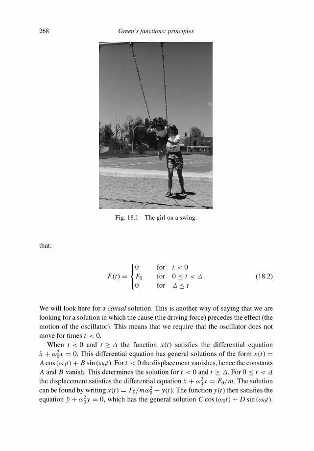
268 Green’s functions: principles
Fig. 18.1 The girl on a swing.
that:
F(t) =⎧
⎨
⎩
0 for t < 0F0 for 0 ≤ t < ∆
0 for ∆ ≤ t. (18.2)
We will look here for a causal solution. This is another way of saying that we arelooking for a solution in which the cause (the driving force) precedes the effect (themotion of the oscillator). This means that we require that the oscillator does notmove for times t < 0.
When t < 0 and t ≥ ∆ the function x(t) satisfies the differential equationx + ω2
0x = 0. This differential equation has general solutions of the form x(t) =A cos (ω0t) + B sin (ω0t). For t < 0 the displacement vanishes, hence the constantsA and B vanish. This determines the solution for t < 0 and t ≥ ∆. For 0 ≤ t < ∆
the displacement satisfies the differential equation x + ω20x = F0/m. The solution
can be found by writing x(t) = F0/mω20 + y(t). The function y(t) then satisfies the
equation y + ω20 y = 0, which has the general solution C cos (ω0t) + D sin (ω0t).

18.1 Girl on a swing 269
This means that the general solution x(t) of the oscillator is given by
x(t) =⎧
⎨
⎩
0 for t < 0F0/mω2
0 + C cos (ω0t) + D sin (ω0t) for 0 ≤ t < ∆
A cos (ω0t) + B sin (ω0t) for ∆ ≤ t, (18.3)
where A, B, C , and D are integration constants which are not yet known.These integration constants follow from the requirement that the displacement
x(t) of the oscillator is at all times continuous and that the velocity x(t) of the os-cillator is at all times continuous. The last condition follows from the considerationthat when the force is finite, the acceleration is finite and the velocity therefore iscontinuous. The requirement that both x(t) and x(t) are continuous at t = 0 and att = ∆ leads to the following equations:
F0/mω20 + C = 0,
ω0 D = 0,
F0/mω20 + C cos (ω0∆) + D sin (ω0∆) = A cos (ω0∆) + B sin (ω0∆),−C sin (ω0∆) + D cos (ω0∆) = −A sin (ω0∆) + B cos (ω0∆).
⎫
⎪
⎪
⎬
⎪
⎪
⎭
(18.4)
These equations are four linear equations for the four unknown integration constantsA, B, C , and D. The upper two equations can be solved directly for the constantsC and D to give the values C = − (
F0/mω20
)
and D = 0. These values for Cand D can then be inserted into the lower two equations. Solving these equationsfor the constants A and B gives the values A = − (
F0/mω20
)
[1 − cos (ω0∆)] andB = (
F0/mω20
)
sin (ω0∆). Inserting these values of the constants into (18.3) showsthat the motion of the oscillator is given by:
x(t) =⎧
⎨
⎩
0 for t < 0(F0/mω2
0) [1 − cos (ω0t)] for 0 ≤ t < ∆.
(F0/mω20) cos [ω0 (t − ∆)] − cos (ω0t) for ∆ ≤ t
(18.5)
This is the solution for a push of duration ∆ delivered at time t = 0. Supposenow that the push is short compared to the period of the oscillator, then ω0∆ 1.In that case one can use a Taylor expansion in ω0∆ for the term cos [ω0 (t − ∆)] in(18.5). This can be achieved by using that cos [ω0 (t − ∆)] = cos (ω0t) cos (ω0∆) −sin (ω0t) sin (ω0∆) and by using the Taylor expansions sin x = x − x3/6 + O(x5)and cos x = 1 − x2/2 + O(x4) for sin (ω0∆) and cos (ω0∆). Retaining only theterm of order (ω0∆) and ignoring terms of higher order in (ω0∆) shows that for animpulsive push (ω0∆ 1) the solution is given by:
x(t) =
0 for t < 0(F0/mω2
0) (ω0∆) sin (ω0t) for t > ∆. (18.6)

270 Green’s functions: principles
We will not bother anymore with the solution between 0 ≤ t < ∆ because in thelimit ∆ → 0 this interval is of vanishing duration.
At this point we have all the ingredients needed to determine the response ofthe oscillator for a general driving force F(t). Suppose we divide the time-axis inintervals of duration ∆. In the i th interval, the force is given by Fi = F(ti ), whereti is the time of the i th interval. We know from (18.6) the response to a force ofduration ∆ at time t = 0. The response to a force Fi at time ti follows by replacingF0 by Fi and by replacing t by t − ti . Making these replacements it thus followsthat the response to a force Fi delivered over a time interval ∆ at time ti is givenby:
x(t) =⎧
⎨
⎩
0 for t < ti1
mω0sin [ω0 (t − ti )] F(ti )∆ for t > ti
. (18.7)
This is the response due to the force acting at time ti only. To obtain the responseto the full force F(t) one should sum over the forces delivered at all times ti . Inthe language of the girl on the swing one would say that (18.6) gives the motion ofthe swing for a single impulsive push, and that we want to use this result to find thedisplacement caused by a number of pushes. Since the differential equation (18.1)is linear we can use the superposition principle which states that the response tothe superposition of two pushes is the sum of the response to the individual pushes.(In the language of Section 15.7 we would say that the swing is a linear system.)This means that when the swing receives a number of pushes at different times tithe response can be written as the sum of the responses to every individual push.With (18.7) this gives:
x(t) =∑
ti <t
1
mω0sin [ω0 (t − ti )] F(ti )∆. (18.8)
Note that in (18.7) the response to a push at time t , before the push at time ti ,vanishes. For this reason one needs to sum in (18.8) only over the pushes at earliertimes because the pushes at later times give a vanishing contribution. For this reasonthe summation is limited to times t ≥ ti .
Suppose now that the swing is not given a finite number of impulse pushes butinstead that the driving force is a continuous function. This case can be handled bytaking the limit ∆ → 0. The summation in (18.8) then needs to be replaced by anintegration. This can naturally be achieved because the duration ∆ is then equal tothe infinitesimal interval dt used in the integration. What we are really doing hereis replacing the continuous function F(t) by a function that is constant within everyinterval ∆ at times ti , see Figure 18.2, and then taking the limit where the widthof the intervals goes to zero, that is ∆ → 0. A similar treatment may be familiar to
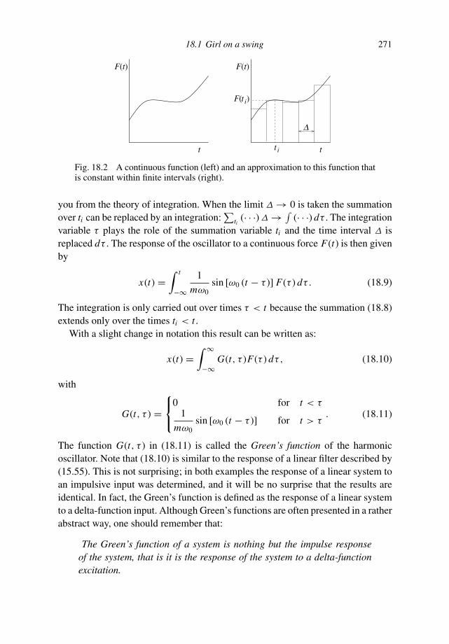
18.1 Girl on a swing 271
t i
t i
F(t)
t
F(t)
t
F( )
Fig. 18.2 A continuous function (left) and an approximation to this function thatis constant within finite intervals (right).
you from the theory of integration. When the limit ∆ → 0 is taken the summationover ti can be replaced by an integration:
∑
ti(· · ·) ∆ → ∫
(· · ·) dτ . The integrationvariable τ plays the role of the summation variable ti and the time interval ∆ isreplaced dτ . The response of the oscillator to a continuous force F(t) is then givenby
x(t) =∫ t
−∞
1
mω0sin [ω0 (t − τ )] F(τ ) dτ . (18.9)
The integration is only carried out over times τ < t because the summation (18.8)extends only over the times ti < t .
With a slight change in notation this result can be written as:
x(t) =∫ ∞
−∞G(t, τ )F(τ ) dτ , (18.10)
with
G(t, τ ) =⎧
⎨
⎩
0 for t < τ1
mω0sin [ω0 (t − τ )] for t > τ
. (18.11)
The function G(t, τ ) in (18.11) is called the Green’s function of the harmonicoscillator. Note that (18.10) is similar to the response of a linear filter described by(15.55). This is not surprising; in both examples the response of a linear system toan impulsive input was determined, and it will be no surprise that the results areidentical. In fact, the Green’s function is defined as the response of a linear systemto a delta-function input. Although Green’s functions are often presented in a ratherabstract way, one should remember that:
The Green’s function of a system is nothing but the impulse responseof the system, that is it is the response of the system to a delta-functionexcitation.

272 Green’s functions: principles
18.2 You have seen Green’s functions before!
Although the concept of a Green’s function may appear to be new to you, you havealready seen several examples of Green’s functions. One example is the electricfield generated by a point charge q at the origin which was treated in Section 6.1:
E(r) = q r4πε0r2
. (6.2)
Since this is the electric field generated by a delta-function charge at the origin, itis closely related to the Green’s function for this problem. The field equation (6.23)of the electric field is invariant for translations in space. This is a complex wayof saying that the electric field depends only on the relative positions of the pointcharge and the point of observation.
Problem a Show that this implies that the electric field at location r due to a pointcharge at location r′ is given by:
E(r) = q
4πε0
(
r − r′)
|r − r′|3 . (18.12)
Now suppose that we do not have a single point charge, but instead a system ofpoint charges qi at locations ri . Since the field equation is linear, the electric fieldgenerated by a sum of point charges is the sum of the fields generated by each pointcharge:
E(r) =∑
i
qi
4πε0
(r − ri )
|r − ri |3. (18.13)
Problem b To which expression of the previous section does this equation cor-respond?
Just as in the previous section we now make the transition from a finite number ofdiscrete inputs (either pushes of the swing or point charges) to an input functionthat is a continuous function (either the applied force to the oscillator as a functionof time or a continuous electric charge). Let the electric charge per unit volume bedenoted by ρ(r). This means that the electric charge in a volume dV is given byρ(r)dV .
Problem c Replace the sum in (18.13) by an integration over volume and use theappropriate charge for each volume element dV to show that the electric field
18.3 Green’s functions as impulse response 273
for a continuous charge distribution is given by:
E(r) =∫∫∫
ρ(r′)4πε0
(
r − r′)
|r − r′|3 dV ′, (18.14)
where the volume integration is over r′.
Problem d Show that this implies that the electric field can be written as
E(r) =∫∫∫
G(r, r′)ρ(r′) dV ′, (18.15)
with the Green’s function given by
G(r, r′) = 1
4πε0
(
r − r′)
|r − r′|3 . (18.16)
Note that this Green’s function has the same form as the electric field for a pointcharge given in (18.12). Note that the Green’s function is only a function of therelative distance r − r′.
Problem e Explain why the integral (18.15) can be seen as a three-dimensionalconvolution: E(r) = ∫∫∫
G(r − r′)ρ(r′)dV ′.
The main purpose of this section is not to show you that you had seen an example ofa Green’s function before. Rather, it provides an example that the Green’s function isnot necessarily a function of time and that it is not necessarily a scalar function; theGreen’s function (18.16) depends on the position but not on time, and it describesa vector field rather than a scalar. The most important thing to remember is that theGreen’s function is the impulse response of a linear system.
Problem f You have seen another Green’s function before if you worked throughSection 17.4 where the response of a particle in syrup was treated. Find theGreen’s function in that section and spot the expressions equivalent to (18.10)and (18.11).
18.3 Green’s function as impulse response
You may have found the derivation of the Green’s function in Section 18.1 rathercomplex. The reason for this is that in (18.3) the motion of the swing was determinedbefore the push (t < 0), during the push (0 < t < ∆) and after the push (t > ∆).The requirement that the displacement x and the velocity x were continuous thenled to the system of equations (18.4) with four unknowns. However, in the end we

274 Green’s functions: principles
took the limit ∆ → 0 and did not use the solution for time 0 < t < ∆. This suggeststhat this method of solution is unnecessarily complicated. This is indeed the case.In this section an alternative derivation of the Green’s function (18.11) is givenwhich is based on the idea that the Green’s function G(t, τ ) describes the motionof the oscillator due to a delta-function force at time τ :
G(t, τ ) + ω20G(t, τ ) = 1
mδ(t − τ ). (18.17)
Problem a For t = τ the delta function vanishes and the right-hand side of thisexpression is equal to zero. We are looking for the causal Green’s function,that is the solution where the cause (the force) precedes the effect (the motionof the oscillator). Show that these conditions imply that for t = τ the Green’sfunction is given by:
G(t, τ ) =
0 for t < τ
A cos[ω0(t − τ )] + B sin[ω0(t − τ )] for t > τ, (18.18)
where A and B are unknown integration constants.
The integration constants follow from the conditions at t = τ . Since we have twounknown parameters we need to impose two conditions. The first condition is thatthe displacement of the oscillator is continuous at t = τ . If this were not the casethe velocity of the oscillator would be infinite at that moment.
Problem b Show that the requirement of continuity of the Green’s function att = τ implies that A = 0.
The second condition requires more care. We derive the second condition firstmathematically and then explore its physical meaning. The second condition fol-lows by integrating (18.17) over t from τ − ε to τ + ε and by taking the limit ε ↓ 0.Integrating (18.17) in this way gives:
∫ τ+ε
τ−ε
G(t, τ ) dt + ω20
∫ τ+ε
τ−ε
G(t, τ ) dt = 1
m
∫ τ+ε
τ−ε
δ(t − τ ) dt. (18.19)
Problem c Show that the right-hand side of (18.19) is equal to 1/m, regardlessof the value of ε.
Problem d Show that the absolute value of the second term on the left-hand sideof (18.19) is smaller than 2εω2
0 max (G), where max (G) is the maximum of
18.3 Green’s functions as impulse response 275
G over the integration interval. Since the Green’s function is finite this meansthat the middle term vanishes in the limit ε ↓ 0.
Problem e Show that the first term on the left-hand side of (18.19) is equalto G(t = τ + ε, τ ) − G(t = τ − ε, τ ). This quantity will be denoted by[G(t, τ )]t=τ+ε
t=τ−ε.
Problem f Use this result to show that in the limit ε ↓ 0 expression (18.19) gives:
[
G(t, τ )]t=τ+ε
t=τ−ε= 1
m. (18.20)
Problem g Show that this condition together with the continuity of G implies thatthe integration constants in (18.18) have the values A = 0 and B = 1/mω0,that is that the Green’s function is given by:
G(t, τ ) =⎧
⎨
⎩
0 for t < τ1
mω0sin [ω0 (t − τ )] for t > τ
. (18.21)
A comparison with (18.11) shows that the Green’s function derived in this sectionis identical to the Green’s function derived in Section 18.1. Note that the solutionwas obtained here without invoking the motion of the oscillator during the momentof excitation. This would have been difficult because the duration of the excitation(a delta function) is equal to zero, if it can be defined at all.
There is, however, something strange about the derivation in this section. InSection 18.1 the solution was found by requiring that the displacement x and itsfirst derivative x were continuous at all times. As used in problem b the first conditionis also met by the solution (18.21). However, the derivative G is not continuous att = τ .
Problem h Which of the equations that you derived above states that the firstderivative is not continuous?
Problem i G(t, τ ) denotes the displacement of the oscillator. Show that expres-sion (18.20) states that the velocity of the oscillator changes discontinuouslyat t = τ .
Problem j Give a physical reason why the velocity of the oscillator was contin-uous in the first part of Section 18.1 and why the velocity is discontinuousfor the Green’s function derived in this section. Hint: how large is the force

276 Green’s functions: principles
needed to produce a finite jump in the velocity of a particle when the forceis applied over a time-interval of length zero (the width of the delta-functionexcitation).
How can we reconcile this result with the solution obtained in Section 18.1?
Problem k Show that the change in the velocity in the solution x(t) in (18.7) isproportional to F(ti )∆, that is that
[x]ti +εti −ε = 1
mF(ti )∆. (18.22)
This means that the change in the velocity depends on the strength of the forcetimes the duration of the force. The physical reason for this is that the change inthe velocity depends on the integral of the force over time divided by the mass ofthe particle.
Problem l Derive this last statement directly from Newton’s law (F = ma).
When the force is finite and when ∆ → 0, the jump in the velocity is zero and thevelocity is continuous. However, when the force is infinite (as is the case for a deltafunction), the jump in the velocity is nonzero and the velocity is discontinuous.
In many applications the Green’s function is the solution of a differential equa-tion with a delta function as the excitation. This implies that some derivative, orcombination of derivatives, of the Green’s function is equal to a delta function at thepoint (or time) of excitation. This usually has the effect that the Green’s functionor its derivative is not a continuous function. The delta function in the differentialequation usually leads to a singularity in the Green’s function or its derivative.
18.4 Green’s function for a general problem
In this section, the theory of Green’s functions is treated in a more abstract fashion.Every linear differential equation for a function u with a source term F can bewritten symbolically as:
Lu = F. (18.23)
For example in (18.1) for the girl on the swing, u is the displacement x(t) whileL is a differential operator given by
L = md2
dt2+ mω2
0, (18.24)
18.4 Green’s functions for a general problem 277
where it is understood that a differential operator acts term by term on the functionto the right of the operator.
Problem a Find the differential operator L and the source term F for the electricfield treated in Section 18.2 from the field equation (6.23).
In the notation used in this section, the Green’s function depends on the positionvector r, but the results derived here are equally valid for a Green’s function thatdepends only on time or on position and time. In general, the differential equation(18.23) must be supplemented with boundary conditions to give a unique solution.In this section the position of the boundary is denoted by rB and it is assumed thatthe function u has the value u B at the boundary:
u(rB) = u B . (18.25)
Let us first find a single solution to the differential equation (18.23) with-out bothering about boundary conditions. We follow the same treatment as inSection 15.7 where in (15.54) the input of a linear function was written as asuperposition of delta functions. In the same way, the source function can bewritten as:
F(r) =∫
δ(r − r′)F(r′) dV ′. (18.26)
This expression follows from the properties of the delta function. One can interpretthis expression as an expansion of the function F(r) in delta functions because theintegral (18.26) describes a superposition of delta functions δ(r − r′) centered atr = r′; each of these delta functions is given a weight F(r′). We want to use a Green’sfunction to construct a solution. The Green’s function G(r, r′) is the response atlocation r due to a delta-function source at location r′, that is the Green’s functionsatisfies:
LG(r, r′) = δ(r − r′). (18.27)
The response to the input δ(r − r′) is given by G(r, r′), and the source functionscan be written as a superposition of these delta functions with weight F(r′). Thissuggests that a solution of (18.23) is given by a superposition of Green’s functionsG(r, r′), where each Green’s function has the same weight factor as the delta func-tion δ(r − r′) in the expansion (18.26) of F(r) in delta functions. This means thata solution of (18.23) is given by:
u P (r) =∫
G(r, r′)F(r′) dV ′. (18.28)
278 Green’s functions: principles
Problem b If you worked through Section 15.7 discuss the relation between thisexpression and (15.55) for the output of a linear function.
It is crucial to understand at this point that we have used three steps to arrive at(18.28): (i) the source function is written as a superposition of delta functions, (ii)the response of the system to each delta-function input is defined, and (iii) thesolution is written as the same superposition of Green’s function as was used in theexpansion of the source function in delta functions:
δ(r − r′) ↔ F(r)(i)= ∫
δ(r − r′)F(r′) dV ′
⇓ (ii) ⇓G(r, r′) ↔ u P (r)
(iii)= ∫
G(r, r′)F(r′) dV ′. (18.29)
Problem c Although this reasoning may sound plausible, we have not proved thatu P (r) in (18.28) actually is a solution of the differential equation (18.23). Givea proof that this is indeed the case by letting the operator L act on (18.28) andby using (18.27) for the Green’s function. Hint: the operator L acts on r whilethe integration is over r′, the operator can thus be taken inside the integral.
It should be noted that we have not solved our problem yet, because u P doesnot necessarily satisfy the boundary conditions. In fact, (18.28) is just one of themany possible solutions to (18.23). It is a particular solution of the inhomogeneousequation (18.23), and this is the reason why the subscript P is used. Equation(18.23) is called an inhomogeneous equation because the right-hand side is nonzero.When the right-hand side is zero one speaks of the homogeneous equation. Thisimplies that a solution uH of the homogeneous equation satisfies
LuH = 0. (18.30)
Problem d In general one can add a solution of the homogeneous equation (18.30)to a particular solution, and the result still satisfies the inhomogeneous equation(18.23). Give a proof of this statement by showing that the function u =u P + uH is a solution of (18.23). In other words show that the general solutionof (18.23) is given by:
u(r) = uH (r) +∫
G(r, r′)F(r′) dV ′. (18.31)
Problem e The problem is that we still need to enforce the boundary conditions(18.25). This can be achieved by requiring that the solution uH satisfies specific
18.5 Radiogenic heating and the Earth’s temperature 279
boundary conditions at rB . Insert (18.31) into the boundary conditions (18.25)and show that the required solution uH of the homogeneous equation mustsatisfy the following boundary conditions:
uH (rB) = u B(rB) −∫
G(rB, r′)F(r′) dV ′. (18.32)
This is all we need to solve the problem. What we have shown is that:
The total solution (18.31) is given by the sum of the particular solution(18.28) plus a solution of the homogeneous equation (18.30) that satisfiesthe boundary condition (18.32).
This construction may appear to be very complex to you. However, you shouldrealize that the main complexity is the treatment of the boundary condition. In manyproblems, the boundary condition dictates that the function vanishes at the boundary(uB = 0) and the Green’s function also vanishes at the boundary. It follows from(18.31) that in that case the boundary condition for the homogeneous solution isu H (rB) = 0. This boundary condition is satisfied by the solution uH (r) = 0, whichimplies that in that case one can dispense with the addition of uH to the particularsolution u P (r).
Problem f Suppose that the boundary conditions do not prescribe the value ofthe solution at the boundary but that instead of (18.25) the normal derivativeof the solution is prescribed by the boundary conditions:
∂u
∂n(rB) = n · ∇u(rB) = wB, (18.33)
where n is the unit vector perpendicular to the boundary. How should thetheory in this section be modified to accommodate this boundary condition?
The theory in this section is rather abstract. In order to make the issues at stake moreexplicit the theory is applied in the next section to the calculation of the temperaturein the Earth.
18.5 Radiogenic heating and the Earth’s temperature
As an application of the use of the Green’s function we consider in this sectionthe calculation of the temperature in the Earth and specifically the effect of thedecay of radioactive elements in the crust on the temperature in the Earth. Severalradioactive elements such as U235 do not fit well in the lattice of mantle rocks. Forthis reason, these elements are expelled from the material in the Earth’s mantle and

280 Green’s functions: principles
Earth’s surfacez = 0T = 0
z = HT = T0
crust Q(z) = Q0
Fig. 18.3 Definition of the geometric variables and boundary conditions for thetemperature in the crust.
they accumulate in the crust. Radioactive decay of these elements then leads to theproduction of heat at the place where these elements have accumulated.
As a simplified example of this problem we assume that the temperature T andthe radiogenic heating Q depend on depth only, and that we can ignore the sphericityof the Earth. In addition, we assume that the radiogenic heating does not dependon time and that we consider only the equilibrium temperature.
Problem a Show that these assumptions imply that the temperature is only afunction of the z-coordinate: T = T (z).
The temperature field satisfies the heat equation derived in Section 11.4:
∂T
∂t= κ∇2T + Q. (11.31)
Problem b Use this expression to show that for the problem in this section thetemperature field satisfies
d2T
dz2= − Q(z)
κ. (18.34)
This equation can be solved when the boundary conditions are specified. The thick-ness of the crust is denoted by H , see Figure 18.3. The temperature is assumed tovanish at the Earth’s surface. In addition, it is assumed that at the base of the crustthe temperature has a fixed value T0.
‡This implies that the boundary conditions
are:
T (z = 0) = 0, T (Z = H ) = T0. (18.35)
In this section we solve the differential equation (18.34) with the boundaryconditions (18.35) using the Green’s function technique described in the previous
‡Geophysically this is an oversimplified boundary condition because in reality the temperature in the Earth isdetermined by the radiogenic heating everywhere in the Earth and by the heat that was formed during the Earth’sformation.

18.5 Radiogenic heating and the Earth’s temperature 281
section. Analogously to (18.28) we first determine a particular solution TP of thedifferential equation (18.34) and worry about the boundary conditions later. TheGreen’s function G(z, z′) to be used is the temperature at depth z due to delta-function heating at depth z′:
d2G(z, z′)dz2
= δ(z − z′). (18.36)
Problem c Use the theory of the previous section to show that the followingfunction satisfies the heat equation (18.34):
TP (z) = − 1
κ
∫ H
0G(z, z′)Q(z′) dz′. (18.37)
Before further progress can be made it is necessary to find the Green’s function,that is to solve the differential equation (18.36). In order to do this the boundaryconditions for the Green’s function need to be specified. In this example we willuse a Green’s function that vanishes at the endpoints of the depth interval:
G(z = 0, z′) = G(Z = H, z′) = 0. (18.38)
Problem d Use (18.36) to show that for z = z′ the Green’s function satisfies thedifferential equation d2G(z, z′)/dz2 = 0 and use this to show that the Green’sfunction which satisfies the boundary conditions (18.38) must be of the form
G(z, z′) =
βz for z < z′
γ (z − H ) for z > z′ , (18.39)
with β and γ constants that need to be determined. These constants are inde-pendent of z, but they may depend on z′.
Problem e Since there are two unknown constants, two conditions are needed.The first condition is that the Green’s function is continuous for z = z′. Usethe theory of Section 18.3 and the differential equation (18.36) to show thatthe second requirement is:
limε↓0
[
dG(z, z′)dz
]z=z′+ε
z=z′−ε
= 1, (18.40)
that is that the first derivative makes a unit jump at the point of excitation.

282 Green’s functions: principles
Problem f Apply these two conditions to the solution (18.39) to determine theconstants β and γ and show that the Green’s function is given by:
G(z, z′) =
⎧
⎪
⎪
⎪
⎨
⎪
⎪
⎪
⎩
− 1
H(H − z′)z for z < z′
− 1
Hz′(H − z) for z > z′
. (18.41)
In this notation the two regions z < z′ and z > z′ are separated. Note, however, thatthe solution in the two regions has a highly symmetric form. In the literature youwill find that a solution such as (18.41) is often rewritten by defining z> to be themaximum of z and z′ and z< to be the minimum of z and z′:
z> ≡ max(z, z′),z< ≡ min(z, z′).
(18.42)
Problem g Show that in this notation the Green’s function (18.41) can be writtenas:
G(z, z′) = − 1
H(H − z>)z<. (18.43)
For simplicity we assume that the radiogenic heating is constant in the crust:
Q(z) = Q0 for 0 < z < H. (18.44)
Problem h Show that the particular solution (18.37) for this heating function isgiven by
TP (z) = Q0 H 2
2κ
z
H
(
1 − z
H
)
. (18.45)
Problem i Show that this particular solution satisfies the boundary conditions
TP (z = 0) = TP (z = H ) = 0. (18.46)
Problem j This means that this solution does not satisfy the boundary conditions(18.35) of our problem. Use the theory in Section 18.4 to show that to obtainthis solution we must add a solution TH (z) of the homogeneous equationd2TH/dz2 = 0 which satisfies the boundary conditions TH (z = 0) = 0 andTH (z = H ) = T0.
18.5 Radiogenic heating and the Earth’s temperature 283
Problem k Show that the solution of the homogeneous equation is given byTH (z) = T0z/H and that the total solution is given by
T (z) = T0z
H+ Q0 H 2
2κ
z
H
(
1 − z
H
)
. (18.47)
Problem l Verify explicitly that this solution satisfies the differential equation(18.34) with the boundary conditions (18.35).
As shown in expression (11.29) the conductive heat flow is given by J = −κ∇T .Since the problem is one-dimensional the heat flow is given by
J = −κdT
dz. (18.48)
Problem m Compute the heat flow at the top (z = 0) and at the bottom (z = H )of the crust. Assuming that T0 and Q0 are both positive, does the heat flowat these locations increase or decrease because of the radiogenic heating Q0?Give a physical interpretation of this result.
The derivation in this section used a Green’s function which satisfies the boundaryconditions (18.38) rather than the boundary conditions (18.35) of the temperaturefield. However, there is no particular reason why one should use these boundaryconditions for the Green’s function. That is to say, one might think one could avoidthe step of adding a solution TH (z) of the homogeneous equation by using a Green’sfunction G that satisfies the differential equation (18.39) and an inhomogeneousboundary condition at the base of the crust:
G(z = 0, z′) = 0, G(z = H, z′) = H. (18.49)
(The boundary value at the base of the crust is set equal to H because the Green’sfunction has the dimension of length (see (18.41)) and the crustal thickness H isthe only length-scale in the problem.)
Problem n Go through the same steps as you did earlier in this section by con-structing the Green’s function G(z, z′), computing the corresponding partic-ular solution TP (z), verifying whether the boundary conditions (18.35) aresatisfied by this particular solution and if necessary adding a solution of thehomogeneous equation in order to satisfy the boundary conditions. Show thatthis again leads to (18.47).

284 Green’s functions: principles
The lesson to be learned from this section is that usually one needs to add a solutionof the homogeneous equation to a particular solution in order to satisfy the boundaryconditions. However, suppose that the boundary conditions of the temperature fieldwere also homogeneous: T = (z = 0) = T (z = H ) = 0. In that case the particularsolution (18.45) that was constructed using a Green’s function that satisfies thehomogeneous boundary conditions (18.38) satisfies the boundary conditions ofthe full problem as well. This implies that it only pays to use a Green’s functionthat satisfies the boundary conditions of the full problem when these boundaryconditions are homogeneous, that is when the function itself vanishes (T = 0) orwhen the normal gradient of the function vanishes (∂T/∂n = 0) or when a linearcombination of these quantities vanishes (aT + b∂T/∂n = 0). In all other cases onecannot avoid adding a solution of the homogeneous equation in order to satisfy theboundary conditions and the most efficient procedure is usually to use the Green’sfunction that can most easily be computed.
18.6 Nonlinear systems and Green’s functions
Up to this point, Green’s functions have been applied to linear systems. The defini-tion of a linear system was introduced in Section 15.7. Suppose that a force F1 leadsto a response x1 and that a force F2 leads to a response x2. A system is linear whenthe response to the linear combination c1 F1 + c2 F2 (with c1 and c2 constants) is thesuperposition response c1x1 + c2x2. This definition implies that the response to theinput times a constant is given by the response multiplied by the same constant. Inother words show that for a linear system an input that is twice as large leads to aresponse that is twice as large.
Problem a Show that the definition of linearity given above implies that the re-sponse to the sum of two force functions is the sum of the responses to theindividual force functions.
This last property reflects that a linear system satisfies the superposition principlewhich states that for a linear system one can superpose the response to a sum offorce functions.
Not every system is linear, and we exploit here the extent to which Green’sfunctions are useful for nonlinear systems. As an example we consider the Verhulstequation:
x = x − x2 + F(t). (18.50)
18.6 Nonlinear systems and the Green’s functions 285
This equation has been used in mathematical biology to describe the growth ofa population. Suppose that only the term x were present on the right-hand side.In that case the solution would be given by x(t) = Cet . This means that the firstterm on the right-hand side accounts for the exponential population growth whichis due to the fact that the number of offspring is proportional to the size of thepopulation. However, a population cannot grow indefinitely; when a populationis too large limited resources restrict the growth, and this is accounted for by the−x2 term on the right-hand side. The term F(t) accounts for external influences onthe population. For example, a mass-extinction could be described by a stronglynegative forcing function F(t). We will consider first the solution for the case thatF(t) = 0. Since the population size is positive we consider positive solutions x(t)only.
Problem b Show that for the case F(t) = 0 the change of variable y = 1/x leadsto the linear equation y = 1 − y. Solve this equation and show that the generalsolution of (18.50) (with F(t) = 0) is given by:
x(t) = 1
Ae−t + 1, (18.51)
with A an integration constant.
Problem c Use this solution to show that any solution of the unforced equationgoes to 1 for infinite times:
limt→∞ x(t) = 1. (18.52)
In other words, the population of the unforced Verhulst equation always convergesto the same population size. Note that when the force vanishes after a finite time,the solution after that time must satisfy (18.51) which implies that the long-timelimit is then also given by (18.52).
Now, consider the response to a delta-function excitation at time t0 with strengthF0. The associated response g(t, t0) thus satisfies
g − g + g2 = F0 δ(t − t0). (18.53)
Since this function is the impulse response of the system, the notation g is usedin order to bring out the resemblance with the Green’s functions used earlier. Weconsider only causal solutions, that is we require that g(t, t0) vanishes for t < t0:g(t, t0) = 0 for t < t0. For t > t0 the solution satisfies the Verhulst equation withoutforce, hence the general form is given by (18.51). The only task remaining is to
286 Green’s functions: principles
find the integration constant A. This constant follows by a treatment similar to theanalysis of Section 18.3.
Problem d Integrate (18.53) over t from t0 − ε to t0 + ε, take the limit ε ↓ 0 andshow that this leads to the following requirement for the discontinuity in g:
limε↓0
[g(t, t0)]t0+εt0−ε = F0. (18.54)
Problem e Use this condition to show that the constant A in the solution (18.51)is given by A = (1/F0 − 1)et0 and that the solution is given by:
g(t, t0) =⎧
⎨
⎩
0 for t < t0F0
(1 − F0)e−(t−t0) + F0for t > t0
. (18.55)
At this point you should be suspicious of interpreting g(t, t0) as a Green’s function.An important property of linear systems is that the response is proportional to theforce. However, the solution g(t, t0) in (18.55) is not proportional to the strengthF0 of the force.
Let us now check whether we can use the superposition principle. Suppose theforce function is the superposition of a delta-function force F1 at t = t1 and adelta-function force F2 at t = t2:
F(t) = F1δ(t − t1) + F2δ(t − t2). (18.56)
By analogy with (18.10) you might think that a Green’s function-type solution isgiven by:
xGreen(t) = F1
(1 − F1)e−(t−t1) + F1+ F2
(1 − F2)e−(t−t2) + F2, (18.57)
for times larger than both t1 and t2. You can verify by direct substitution that thisfunction is not a solution of the differential equation (18.50). However, this processis rather tedious and there is a simpler way to see that the function xGreen(t) violatesthe differential equation (18.50).
Problem f To see this, show that the solution xGreen(t) has the following long-timebehavior:
limt→∞ xGreen(t) = 2. (18.58)

18.6 Nonlinear systems and the Green’s functions 287
This limit is at odds with the limit (18.52) that every solution of the differentialequation (18.50) should satisfy when the force vanishes after a certain finite time.This proves that xGreen(t) is not a solution of the Verhulst equation.
This implies that the Green’s function technique introduced in the previous sec-tions cannot be used for a nonlinear equation such as the forced Verhulst equation.The reason for this is that Green’s functions are based on the superposition princi-ple; by knowing the response to a delta-function force and by writing a general forceas a superposition of delta functions one can construct a solution by making thecorresponding superposition of Green’s functions, see (18.29). However, solutionsof a nonlinear equation such as the Verhulst equation do not satisfy the principle ofsuperposition. This implies that Green’s function cannot be used effectively to con-struct the behavior of nonlinear systems. It is for this reason that Green’s functionsare in practice only used for constructing the response of linear systems.

19
Green’s functions: examples
In the previous chapter the basic theory of Green’s function was introduced. In thischapter a number of examples of Green’s functions are shown that are often usedin mathematical physics.
19.1 Heat equation in N dimensions
In this section we consider once again the heat equation as introduced in Sec-tion 11.4:
∂T
∂t= κ∇2T + Q. (11.31)
First we construct a Green’s function for this equation in N space dimensions. Thereason for this is that the analysis for N dimensions is just as easy (or difficult) asthe analysis for only one spatial dimension.
The heat equation is invariant for translations in both space and time. For thisreason the Green’s function G(r,t ; r0, t0) that gives the temperature at locationr and time t due to a delta-function heat source at location r0 and time t0 de-pends only on the relative distance r − r0 and the relative time t − t0. This impliesthat G(r,t ; r0, t0) = G(r − r0, t − t0). Since the Green’s function depends only onr − r0 and t − t0 it suffices to construct the simplest solution by considering thespecial case of a source at r0 = 0 at time t0 = 0. This means that we construct theGreen’s function G(r,t) that satisfies:
∂G(r,t)∂t
− κ∇2G(r,t) = δ(r)δ(t). (19.1)
This Green’s function can most easily be constructed by carrying out a spatialFourier transform. Using the Fourier transform (15.27) for each of the N spatial
288
19.1 Heat equation in N dimensions 289
dimensions one finds that the Green’s function has the following Fourier expansion:
G(r, t) = 1
(2π)N
∫
g(k, t)eik·rd N k. (19.2)
Note that the Fourier transform is only carried out over the spatial dimensions andnot over time. This implies that g(k, t) is a function of time as well. The differentialequation that g satisfies can be obtained by inserting the Fourier representation(19.2) in the differential equation (19.1). In doing this we also need the Fourierrepresentation of ∇2G(r,t).
Problem a Show by applying the Laplacian to the Fourier integral (19.1) that:
∇2G(r, t) = −1
(2π)N
∫
k2g(k, t)eik·rd N k. (19.3)
Problem b As a last ingredient we need the Fourier representation of the deltafunction on the right-hand side of (19.1). This multi-dimensional delta func-tion is a shorthand notation for δ(r) = δ(x1)δ(x2) · · · δ(xN ). Use the Fourierrepresentation (15.31) of the delta function to show that:
δ(r) = 1
(2π)N
∫
eik·rd N k. (19.4)
Problem c Insert these results into the differential equation (19.1) of the Green’sfunction to show that g(k, t) satisfies the differential equation
∂g(k, t)
∂t+ κk2g(k, t) = δ(t). (19.5)
We have made considerable progress. The original equation (19.1) was a partialdifferential equation, whereas (19.5) is an ordinary differential equation for g be-cause only a time derivative is taken. In fact, you saw this equation before whenyou read Section 17.4 which dealt with the response of a particle in syrup. Equation(19.5) is equivalent to the equation of motion (17.28) for a particle in syrup whenthe forcing force is a delta function.
Problem d Use the theory of Section 18.3 to show that the causal solution of(19.5) is given by:
g(k, t) = e−κk2t . (19.6)
290 Green’s functions: examples
This solution can be inserted into the Fourier representation (19.2) of the Green’sfunction, and this gives:
G(r, t) = 1
(2π)N
∫
e−κk2t+ik·rd N k. (19.7)
The Green’s function can be found by solving this Fourier integral. Before wedo this, let us pause to consider the solution (19.6) for the Green’s function inthe wavenumber–time domain. The function g(k, t) gives the coefficient of theplane wave component eik·r as a function of time. According to (19.6) each Fouriercomponent decays exponentially with time with a characteristic decay time 1/κk2.
Problem e Show that this implies that in the Fourier expansion (19.2) plane waveswith a smaller wavelength decay faster with time than plane waves with a largerwavelength. Explain this result physically.
In order to find the Green’s function, we need to solve the Fourier integral (19.7).The integrations over the different components ki of the wavenumber integrationall have the same form.
Problem f Show this by giving a proof that the Green’s function can be writtenas:
G(r, t) = 1
(2π)N
(∫
e−κk21 t+ik1x1dk1
) (∫
e−κk22 t+ik2x2dk2
)
× · · ·(∫
e−κk2N t+ikN xN dkN
)
. (19.8)
You will notice that each of the integrals is of the same form, hence the Green’sfunction can be written as
G(x1, x2, . . . , xN , t) = I (x1, t)I (x2, t) · · · I (xN , t)
with I (x, t) given by
I (x, t) = 1
2π
∫ ∞
−∞e−κk2t+ikx dk. (19.9)
This means that our problem is solved when the one-dimensional Fourier integral(19.9) is solved. In order to solve this integral it is important to realize that theexponent in the integral is a quadratic function of the integration variable k. If theintegral were of the form
∫ ∞−∞ e−αk2
dk the problem would not be difficult because
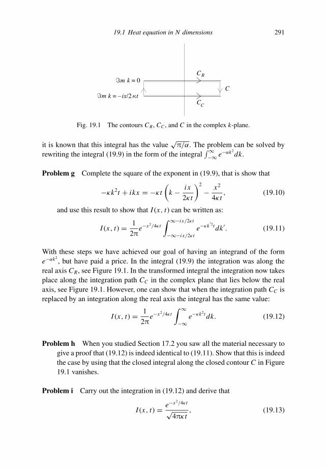
19.1 Heat equation in N dimensions 291
C
C
CC
Rk = 0
Fig. 19.1 The contours CR , CC , and C in the complex k-plane.
it is known that this integral has the value√
π/α. The problem can be solved byrewriting the integral (19.9) in the form of the integral
∫ ∞−∞ e−αk2
dk.
Problem g Complete the square of the exponent in (19.9), that is show that
−κk2t + ikx = −κt
(
k − i x
2κt
)2
− x2
4κt, (19.10)
and use this result to show that I (x, t) can be written as:
I (x, t) = 1
2πe−x2/4κt
∫ ∞−i x/2κt
−∞−i x/2κte−κk
′2t dk ′. (19.11)
With these steps we have achieved our goal of having an integrand of the forme−αk2
, but have paid a price. In the integral (19.9) the integration was along thereal axis CR , see Figure 19.1. In the transformed integral the integration now takesplace along the integration path CC in the complex plane that lies below the realaxis, see Figure 19.1. However, one can show that when the integration path CC isreplaced by an integration along the real axis the integral has the same value:
I (x, t) = 1
2πe−x2/4κt
∫ ∞
−∞e−κk2t dk. (19.12)
Problem h When you studied Section 17.2 you saw all the material necessary togive a proof that (19.12) is indeed identical to (19.11). Show that this is indeedthe case by using that the closed integral along the closed contour C in Figure19.1 vanishes.
Problem i Carry out the integration in (19.12) and derive that
I (x, t) = e−x2/4κt
√4πκt
, (19.13)

292 Green’s functions: examples
and show that this implies that the Green’s function is given by
G(r, t) = 1
(4πκt)N/2 e−r2/4κt . (19.14)
Problem j This result implies that the Green’s function in any dimension has theform of the Gaussian. Show that this Gaussian changes shape with time. Isthe Gaussian broadest at early times or at late times? What is the shape of theGreen’s function in the limit t ↓ 0, that is at the time just after the heat forcehas been applied.
Problem k Sketch the time behavior of the Green’s function for a fixed distancer . Does the Green’s function decay more rapidly as a function of time in threedimensions than in one dimension? Give a physical interpretation of this result.
In one dimension, the Green’s function (19.14) is given by
G(x, t) = 1√4πκt
e−x2/4κt . (19.15)
Problem l Show that this is the same function as the solution (11.41) for the heatequation in one dimension when the limits L → 0 and T0L → 1 are taken.
These limits to the Gaussian function define the delta function, see Section 14.1.This explains why in this limit the Green’s function (19.15) and solution (11.41)are identical.
It is a remarkable property of the derivation in this section that the Green’sfunction can be derived with a single derivation for every number of dimensions. Itshould be noted that this is not the generic case. In many problems, the behavior ofthe system depends critically on the number of spatial dimensions. We will see inSection 19.4 that wave propagation in two dimensions is fundamentally differentfrom wave propagation in one or three dimensions. Another example is chaoticbehavior of dynamical systems where the occurrence of chaos is intricately linkedto the number of dimensions, see the discussion given by Tabor [104].
19.2 Schrodinger equation with an impulsive source
In this section we study the Green’s function for the Schrodinger equation whichwas introduced in Section 8.4:
ih∂ψ(r, t)
∂t= − h2
2m∇2ψ(r, t) + V (r)ψ(r, t). (8.14)

19.2 Schrodinger equation with an impulsive source 293
Solving this equation for a general potential V (r) is a formidable problem, andsolutions are known for only very few examples such as the free particle, theharmonic oscillator, and the Coulomb potential. We restrict ourselves here tothe simplest case of a free particle: this is the case where the potential vanishes(V (r) = 0). The corresponding Green’s function satisfies the following partial dif-ferential equation:
h
i
∂G(r, t)
∂t− h2
2m∇2G(r, t) = δ(r)δ(t). (19.16)
Before we compute the Green’s function for this problem, let us pause to considerthe meaning of this Green’s function. First, the Green’s function is a solution ofSchrodinger’s equation for r = 0 and t = 0. This means that |G|2 gives the prob-ability density of a particle (see also Section 8.4). However, the right-hand side of(19.16) contains a delta-function forcing at time t = 0 at location r = 0. This is asource term of G and hence this is a source of the probability of the presence ofthe particle. One can say that this source term creates the probability for having aparticle at the origin at t = 0. Of course, this particle will not necessarily remain atthe origin, it will move according to the laws of quantum mechanics. This motionis described by (19.16). This means that this equation describes the time evolutionof matter waves when matter is injected at t = 0 at location r = 0.
Problem a The Green’s function G(r, t ; r′, t ′) gives the wavefunction at locationr and time t for a source of particles at location r′ at time t ′. Express theGreen’s function G(r, t ; r′, t ′) in terms of the solution G(r, t) of (19.16), andshow how you obtained this result. Is this result also valid for the Green’sfunction for the quantum-mechanical harmonic oscillator (where the potentialV (r) depends on position)?
In the previous section the Green’s function gave the evolution of the temperaturefield due to a delta-function injection of heat at the origin at time t = 0. Similarly,the Green’s function of this section describes the time evolution of the probabilityof a delta-function injection of matter waves at the origin at time t = 0. These twoGreen’s functions are not only conceptually very similar, the differential equations(19.1) for the temperature field and (19.16) for the Schrodinger equation are firstorder differential equations in time and second order differential equations in thespace coordinate that have a delta-function excitation on the right-hand side. In thissection we exploit this similarity and derive the Green’s function for Schrodinger’sequation from the Green’s function for the heat equation derived in the previoussection rather than constructing the solution from first principles. This approach

294 Green’s functions: examples
is admittedly not very rigorous, but it shows that analogies are useful for makingshortcuts.
The principle difference between (19.1) and (19.16) is that the time derivativefor Schrodinger’s equation is multiplied by i = √−1 whereas the heat equation ispurely real. We will relate the two equations by introducing the new time variableτ for the Schrodinger equation that is proportional to the original time: τ = γ t .
Problem b How should the proportionality constant γ be chosen so that (19.16)transforms to:
∂G(r, τ )
∂τ− h2
2m∇2G(r, τ ) = Cδ(r)δ(τ ). (19.17)
The constant C on the right-hand side cannot easily be determined from thechange of variables τ = γ t because γ is not necessarily real and it is not clearhow a delta function with a complex argument should be interpreted. For thisreason we will not bother to specify C .
The key point to note is that this equation is of exactly the same form as the heatequation (19.1), where h2/2m plays the role of the heat conductivity κ . The onlydifference is the constant C on the right-hand side of (19.17). However, since theequation is linear, this term only leads to an overall multiplication by C .
Problem c Show that the Green’s function defined in (19.17) for the Schrodingerequation can be obtained from the Green’s function (19.14) for the heat equa-tion by making the following substitutions:
t −→ i t/h,
κ −→ h2/2m,
G −→ C G.
⎫
⎬
⎭
(19.18)
It is interesting to note that the “diffusion constant” κ which governs the spreadingof the waves with time is proportional to the square of Planck’s constant. Classicalmechanics follows from quantum mechanics by letting Planck’s constant go to zero:h → 0. It follows from (19.18) that in that limit the diffusion constant of the matterwaves goes to zero. This reflects the fact that in classical mechanics the probabilityof the presence of a particle does not spread out with time.
Problem d Use the substitutions (19.18) to show that the Green’s function for theSchrodinger equation in N dimensions is given by:
G(r, t) = C1
(2πiht/m)N/2 eimr2/2ht . (19.19)
19.2 Schrodinger equation with an impulsive source 295
This Green’s function plays a crucial role in the formulation of the Feynman pathintegrals which have been a breakthrough in quantum mechanics as well as in otherfields. A clear description of the Feynman path integrals is given by Feynman andHibbs [40].
Problem e Sketch the real part of eimr2/2ht in the Green’s function for a fixed timeas a function of radius r . Does the wavelength of the Green’s function increaseor decrease with distance?
The Green’s function (19.19) actually has an interesting physical meaning which isbased on the fact that it describes the propagation of matter waves injected at t = 0at the origin. The Green’s function can be written as G = C (2πiht/m)−N/2 ei,where the phase of the Green’s function is given by
= mr2
2ht. (19.20)
As you noted in problem e of Section 8.4 the wavenumber of the waves dependson position. For a plane wave eik·r the phase is given by = (k · r) and the wave-number follows by taking the gradient of this function.
Problem f Show that for a plane wave
k = ∇. (19.21)
Relation (19.21) has a wider applicability than plane waves. It has been shown byWhitham [119] that for a general phase function (r) that varies smoothly with rthe local wavenumber k(r) is defined by (19.21).
Problem g Use this to show that for the Green’s function of the Schrodingerequation the local wavenumber is given by
k =mrht
. (19.22)
Problem h Use the definition v = r/t to show that this expression is equivalentto:
v =hkm
. (8.21)
In problem e you discovered that for a fixed time, the wavelength of the wavesdecreases when the distance r to the source is increased. This is consistent with(8.21): when a particle has moved further away from the source in a fixed time, its
296 Green’s functions: examples
velocity is larger. This corresponds according to (8.21) with a larger wavenumberand hence with a smaller wavelength. This is indeed the behavior that is exhibitedby the full wave-function (19.19).
The analysis in this chapter was not rigorous because the substitution t → (i/h) timplies that the independent parameter is purely imaginary rather than real. Thismeans that all the arguments used in the previous section for the complex integra-tion should be carefully reexamined. However, a more rigorous analysis shows that(19.19) is indeed the correct Green’s function for the Schrodinger equation [40].The approach taken in this section shows that an educated guess can be very usefulin deriving new results. One can in fact argue that many innovations in mathe-matical physics have been obtained using intuition or analogies rather than formalderivations. Of course, a formal derivation should ultimately substantiate resultsobtained from a more intuitive approach.
19.3 Helmholtz equation in one, two, and three dimensions
The Helmholtz equation plays an important role in mathematical physics because itis closely related to the wave equation. A complete analysis of the Green’s functionfor the wave equation and the Helmholtz equation in different dimensions is givenby DeSanto [34]. The Green’s function for the wave equation for a medium withconstant velocity c satisfies:
∇2G(r, t ; r0, t0) − 1
c2
∂2G(r, t ; r0, t0)
∂t2= δ(r − r0)δ(t − t0). (19.23)
As shown in Section 19.1 the Green’s function depends for a constant velocityc only on the relative location r − r0 and the relative time t − t0 so that withoutloss of generality we can take the source at the origin (r0 = 0) and let the sourceact at time t0 = 0. In addition it follows from symmetry considerations that theGreen’s function depends only on the relative distance |r − r0| and not on theorientation of the vector r − r0. This means that the Green’s function then satisfiesG(r, t ; r0, t0) = G(|r − r0| , t − t0) and we need to solve the following equation:
∇2G(r, t) − 1
c2
∂2G(r, t)
∂t2= δ(r)δ(t). (19.24)
Problem a Under which conditions is this approach justified?
Problem b Use a similar treatment to that in Section 19.1 to show that when theFourier transform (15.43) is used the Green’s function satisfies the following

19.3 Helmholtz equation in one, two, and three dimensions 297
equation in the frequency domain:
∇2G(r, ω) + k2G(r, ω) = δ(r), (19.25)
where the wavenumber k satisfies k = ω/c.
This equation is called the Helmholtz equation and is the reformulation of the waveequation in the frequency domain. In the following we suppress the factor ω in theGreen’s function but it should be remembered that the Green’s function dependson frequency.
Let us first solve (19.25) for one dimension. In that case the Green’s function isdefined by
d2G
dx2+ k2G = δ(x). (19.26)
Problem c For x = 0 the right-hand side of this equation is equal to zero. Usethis to show that for x = 0 the solution is given by
G(x) = A eikx + B e−ikx , (19.27)
where A and B are integration constants which need to be determined for theregions x < 0 and x > 0 separately.
In the Fourier transformation to the time domain, both terms are multiplied bye−iωt . Using the relation k = ω/c, this means that in the time domain the term eikx
becomes e−iω(t−x/c). For increasing time t , the phase of the wave remains constantwhen x increases. This means that the term eikx corresponds in the time domain toa right-going wave. Similarly, the term e−ikx describes a wave in the time domainthat moves to the left. We are looking here for a Green’s function that describeswaves that move away from the source. This means that for x > 0 only the term eikx
contributes, so in that region we must have B = 0, while for x < 0 only the terme−ikx contributes hence we must take A = 0. This means that the Green’s functionis given by
G(x) =⎧
⎨
⎩
B e−ikx for x < 0
A eikx for x > 0. (19.28)
The constants A and B follow from the requirements that G(x) is continuous atx = 0 and that the first derivative is discontinuous at that point.
298 Green’s functions: examples
Problem d Use the theory of Section 18.3 to show that the jump in the firstderivative at x = 0 is given by
[
dG
dx
]x=0+ε
x=0−ε
= 1. (19.29)
Problem e Use these results to derive that A = B = −i/2k, and use this resultto write the Green’s function of the Helmholtz equation in one dimension as
G1D(x) = −i
2keik|x |. (19.30)
Now we solve (19.25) for two and three space dimensions. To do this we con-sider the case of N dimensions, where N is either 2 or 3. Because the problem isspherically symmetric, we just need to consider a Green’s function that depends onradius only.
Problem f Use (10.35) and (10.36) to show that for such a radially symmetricfunction in two or three dimensions the Laplacian is given by
∇2G(r ) = 1
r N−1
∂
∂r
(
r N−1 ∂G
∂r
)
. (19.31)
The differential equation for the Green’s function in N dimensions is thus given by
1
r N−1
∂
∂r
(
r N−1 ∂G
∂r
)
+ k2G(r, ω) = δ(r). (19.32)
This differential equation is not difficult to solve for two or three space dimensionsfor locations away from the source (r = 0). However, we need to consider carefullyhow the source δ(r) should be coupled to the solution of the differential equation.This can be achieved by integrating (19.25) over a sphere of radius R centered atthe source and letting the radius go to zero.
Problem g Integrate (19.25) over this volume, use Gauss’s law and let the radiusR go to zero to show that the Green’s function satisfies
∮
SR
∂G
∂rd S = 1, (19.33)
where the surface integral is over a sphere SR with radius R in the limit R ↓ 0.Show that this can also be written as
limr↓0
Sr∂G
∂r= 1, (19.34)
where Sr is the surface of a sphere in N dimensions with radius r .
19.3 Helmholtz equation in one, two, and three dimensions 299
Note that the surface of the sphere in general goes to zero as r ↓ 0 (except in onedimension), which implies that ∂G/∂r must be infinite in the limit r ↓ 0 in morethan one space dimension.
The differential equation (19.32) is a second order differential equation. Such anequation must be supplemented with two boundary conditions. The first boundarycondition is given by (19.34), and specifies how the solution is coupled to the sourceat r = 0. The second boundary condition that we will use reflects the fact that thewaves generated by the source will move away from the source. The solutions thatwe will find will behave for large distances as e±ikr , but it is not clear whether weshould use the upper sign (+) or the lower sign (−).
Problem h Use the Fourier transform (15.42) and the relation k = ω/c to showthat the integrand in the Fourier transformation to the time domain is propor-tional to e−iω(t∓r/c).
‡Show that the waves only move away from the source for
the upper sign by showing that for this solution the distance r must increasefor increasing time t to keep the phase constant. This means that this boundarycondition dictates that the solution behaves in the limit r → ∞ as e+ikr.
The derivative of function e+ikr is given by ike+ikr, that is the derivative is ik timesthe original function. When the Green’s function behaves for large r as e+ikr, then thederivative of the Green’s function must satisfy the same relation as the derivativeof e+ikr. This means that the Green’s function satisfies for large distance r :
∂G
∂r= ikG. (19.35)
This relation specifies that the energy radiates away from the source. For this reason(19.35) is called the radiation boundary condition.
Now we are at the point where we can actually construct the solution for eachdimension. Before we go to two dimensions we first solve the Green’s function inthree dimensions.
Problem i Make for three dimensions (N = 3) the substitution G(r ) = f (r )/rand show that (19.32) implies that away from the source the function f (r )satisfies
∂2 f
∂r2+ k2 f = 0. (19.36)
This equation has the solution Ce±ikr. According to problem h the upper sign
‡The convention of the notation ∓ is that the upper sign in e−iω(t∓r/c) corresponds to the upper sign in e±ikr .Similarly, the lower signs in both expressions correspond to each other. This means that the solution e−iω(t−r/c)
corresponds to e+ikr and that the solution e−iω(t+r/c) corresponds to e−ikr .

300 Green’s functions: examples
should be used and the Green’s function is given by G(r ) = Ceikr/r . Showthat condition (19.34) dictates that C = −1/4π, so that in three dimensionsthe Green’s function is given by:
G3D(r ) = −1
4π
eikr
r. (19.37)
The problem is actually most difficult in two dimensions because in that casethe Green’s function cannot be expressed in the simplest elementary functions.
Problem j Show that in two dimensions (N = 2) the differential equation of theGreen’s function away from the source is given by
∂2G
∂r2+ 1
r
∂G
∂r+ k2G(r ) = 0, r = 0. (19.38)
Problem k This equation cannot be solved in terms of elementary functions.However, there is a close relation between (19.38) and the Bessel equationthat is given by
d2 F
dx2+ 1
x
d F
dx+
(
1 − m2
x2
)
F = 0. (19.39)
Show that the G(kr ) satisfies the Bessel equation for order m = 0.
This implies that the Green’s function is given by the solution of the zeroth orderBessel equation with argument kr . The Bessel equation is a second order differentialequation, therefore there are two independent solutions. The solution that is finiteeverywhere is denoted by Jm(x) and is called the regular Bessel function. Thesecond solution is singular at the point x = 0 and is called the Neumann functionand denoted by Nm(x). The Green’s function is obviously a linear combination ofJ0(kr ) and N0(kr ). In order to determine how this linear combination is constructedit is crucial to consider the behavior of these functions at the source (i.e. for kr = 0)and at infinity (i.e. for kr 1). The required asymptotic behavior can be found intextbooks such as Butkov [24] and Arfken [5] and is summarized in Table 19.1.
Problem l Show that neither J0(kr ) nor N0(kr ) behaves for large values of r ase+ikr. Show that the linear combination J0(kr ) + i N0(kr ) does behave as e+ikr.
The Green’s function thus is a linear combination of the regular Bessel functionand the Neumann function. This particular combination is called the first Hankelfunction of degree zero and is denoted by H (1)
0 (kr ). The Hankel functions are simply

19.3 Helmholtz equation in one, two, and three dimensions 301
Table 19.1 Leading asymptotic behavior of the Bessel function and Neumannfunction of order zero
J0(x) N0(x)
x → 0 1 − 1
4x2 + O(x4)
2
πln (x) + O(1)
x 1
√
2
πxcos
(
x − π
4
)
+ O(x−3/2)
√
2
πxsin
(
x − π
4
)
+ O(x−3/2)
linear combinations of the Bessel function and the Neumann function:
H (1)m (x) ≡ Jm(x) + i Nm(x),
H (2)m (x) ≡ Jm(x) − i Nm(x).
(19.40)
Problem m Use this definition and Table 19.1 to show that H (1)0 (kr ) behaves for
large values of r as e+ikr−iπ/4/√
(π/2)kr and that in this limit H (2)0 (kr ) behaves
as e−ikr−iπ/4/√
(π/2)kr . Use this to argue that the Green’s function is givenby
G(r ) = C H (1)0 (kr ), (19.41)
where the constant C still needs to be determined.
Problem n This constant follows from the requirement (19.34) at the source. Use(19.40) and the asymptotic value of the Bessel function and the Neumannfunction given in Table 19.1 to derive the asymptotic behavior of the Green’sfunction near the source and use this to show that C = −i/4.
This result implies that in two dimensions the Green’s function of the Helmholtzequation is given by
G2D(r ) = −i
4H (1)
0 (kr ). (19.42)
Summarizing these results and reverting to the more general case of a source atlocation r0 it follows that in one, two, and three dimensions the Green’s functions
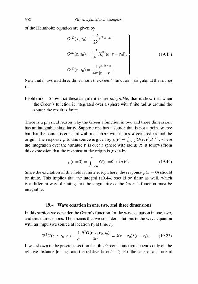
302 Green’s functions: examples
of the Helmholtz equation are given by
G1D(x, x0) = −i
2keik|x−x0|,
G2D(r, r0) = −i
4H (1)
0 (k |r − r0|),
G3D(r, r0) = −1
4π
eik|r−r0|
|r − r0| .
⎫
⎪
⎪
⎪
⎪
⎪
⎪
⎪
⎪
⎪
⎬
⎪
⎪
⎪
⎪
⎪
⎪
⎪
⎪
⎪
⎭
(19.43)
Note that in two and three dimensions the Green’s function is singular at the sourcer0.
Problem o Show that these singularities are integrable, that is show that whenthe Green’s function is integrated over a sphere with finite radius around thesource the result is finite.
There is a physical reason why the Green’s function in two and three dimensionshas an integrable singularity. Suppose one has a source that is not a point sourcebut that the source is constant within a sphere with radius R centered around theorigin. The response p to this source is given by p(r) = ∫
r ′<R G(r, r′)dV ′ , wherethe integration over the variable r′ is over a sphere with radius R. It follows fromthis expression that the response at the origin is given by
p(r =0) =∫
r ′<R
G(r =0, r′) dV
′. (19.44)
Since the excitation of this field is finite everywhere, the response p(r = 0) shouldbe finite. This implies that the integral (19.44) should be finite as well, whichis a different way of stating that the singularity of the Green’s function must beintegrable.
19.4 Wave equation in one, two, and three dimensions
In this section we consider the Green’s function for the wave equation in one, two,and three dimensions. This means that we consider solutions to the wave equationwith an impulsive source at location r0 at time t0:
∇2G(r, t ; r0, t0) − 1
c2
∂2G(r, t ; r0, t0)
∂t2= δ(r − r0)δ(t − t0). (19.23)
It was shown in the previous section that this Green’s function depends only on therelative distance |r − r0| and the relative time t − t0. For the case of a source at
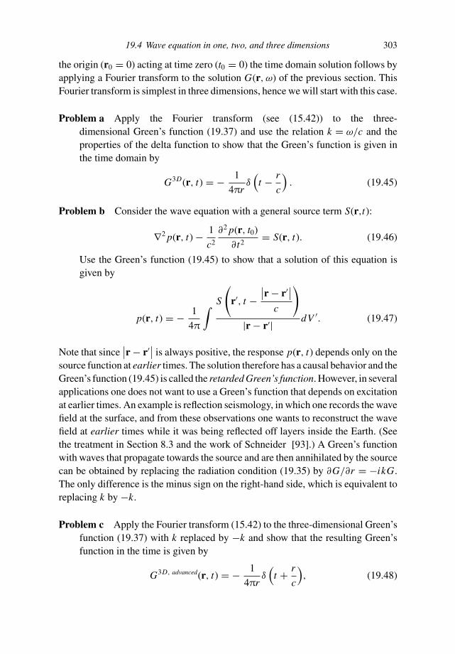
19.4 Wave equation in one, two, and three dimensions 303
the origin (r0 = 0) acting at time zero (t0 = 0) the time domain solution follows byapplying a Fourier transform to the solution G(r, ω) of the previous section. ThisFourier transform is simplest in three dimensions, hence we will start with this case.
Problem a Apply the Fourier transform (see (15.42)) to the three-dimensional Green’s function (19.37) and use the relation k = ω/c and theproperties of the delta function to show that the Green’s function is given inthe time domain by
G3D(r, t) = − 1
4πrδ(
t − r
c
)
. (19.45)
Problem b Consider the wave equation with a general source term S(r,t):
∇2 p(r, t) − 1
c2
∂2 p(r, t0)
∂t2= S(r, t). (19.46)
Use the Green’s function (19.45) to show that a solution of this equation isgiven by
p(r, t) = − 1
4π
∫
S
(
r′, t −∣
∣r − r′∣∣
c
)
|r − r′| dV ′. (19.47)
Note that since∣
∣r − r′∣∣ is always positive, the response p(r, t) depends only on the
source function at earlier times. The solution therefore has a causal behavior and theGreen’s function (19.45) is called the retarded Green’s function. However, in severalapplications one does not want to use a Green’s function that depends on excitationat earlier times. An example is reflection seismology, in which one records the wavefield at the surface, and from these observations one wants to reconstruct the wavefield at earlier times while it was being reflected off layers inside the Earth. (Seethe treatment in Section 8.3 and the work of Schneider [93].) A Green’s functionwith waves that propagate towards the source and are then annihilated by the sourcecan be obtained by replacing the radiation condition (19.35) by ∂G/∂r = −ikG.The only difference is the minus sign on the right-hand side, which is equivalent toreplacing k by −k.
Problem c Apply the Fourier transform (15.42) to the three-dimensional Green’sfunction (19.37) with k replaced by −k and show that the resulting Green’sfunction in the time is given by
G3D, advanced(r, t) = − 1
4πrδ(
t + r
c
)
, (19.48)

304 Green’s functions: examples
and that the following function is a solution of the wave equation (19.46):
p(r, t) = − 1
4π
∫
S
(
t +∣
∣r − r′∣∣
c
)
|r − r′| dV ′. (19.49)
Note that in this representation the wave field is expressed in terms of the sourcefunction at later times. For this reason the Green’s function (19.48) is called theadvanced Green’s function. The fact that the wave equation has both a retardedand an advanced solution is mathematically due to the wave equation (19.46) beinginvariant for time-reversal. This means that when one replaces t by −t the equationdoes not change. Physically this means that the wave equation does not knowthe “direction of time”. In practice one most often works with the retarded Green’sfunction, but keep in mind that in some applications, such as exploration seismology,the advanced Green’s functions are crucial. In the remaining part of this sectionwe will focus exclusively on the retarded Green’s functions that represent causalsolutions.
In order to obtain the Green’s function for two dimensions in the time domainone could apply a Fourier transform to the solution (19.42). This involves taking theFourier transform of a Hankel function, and it is not obvious how this Fourier integralshould be solved (although it can be solved). Here we follow an alternative route byrecognizing that the Green’s function in two dimensions is identical to the solutionof the wave equation in three dimensions when the source is not a point sourcebut a cylindrical source. In other words, we obtain the two-dimensional Green’sfunction by considering the wave field in three dimensions that is generated by asource which is distributed homogeneously along the z-axis. In order to separatethe distance to the origin from the distance to the z-axis the variables r and ρ areused, see Figure 19.2.
Problem d Use this line source to show that
G2D(ρ, t) =∫ ∞
−∞G3D(r, t) dz. (19.50)
Problem e Use the Green’s function (19.45) and the relation
r =√
ρ2 + z2

19.4 Wave equation in one, two, and three dimensions 305
r
r = ρ2+z2
x−axis
y−axis
z−axis
ρ
Fig. 19.2 Definition of the variables r and ρ.
to show that
G2D(ρ, t) = − 1
2π
∫ ∞
0
δ
(
t −√
ρ2 + z2
c
)
√
ρ2 + z2dz. (19.51)
Note that the integration interval has been changed from (−∞,∞) to (0, ∞),and show how this can be achieved.
The distance r in three dimensions no longer appears in this expression.
Problem f The integral (19.51) can be solved by introducing the new integrationvariable u ≡
√
ρ2 + z2 , instead of the old integration variable z. Show thatwith this new variable the integral (19.51) can be written as
G2D(ρ, t) = − 1
2π
∫ ∞
ρ
δ(
t − u
c
)
√
u2 − ρ2du: (19.52)
pay attention to the limits of integration!
Problem g Use the property δ(ax) = δ(x)/ |a| to rewrite this integral and evaluatethe resulting integral separately for t < ρ/c and t > ρ/c. Finally denote thedistance ρ in the two-dimensional (x, y)-plane by r to show that
G2D(r, t) =
⎧
⎪
⎪
⎨
⎪
⎪
⎩
0 for t < r/c
− 1
2π
1√
t2 − r2/c2for t > r/c
. (19.53)

306 Green’s functions: examples
three dimensions
two dimensions
one dimension
t = r/c
Fig. 19.3 The Green’s function of the wave equation in one, two, and threedimensions as a function of time.
This Green’s function and the Green’s function for the three-dimensional case aresketched in Figure 19.3. There is a fundamental difference between the Green’sfunction for two dimensions and the Green’s function (19.45) for three dimensions.In three dimensions the Green’s function is a delta-function δ(t − r/c) modulatedby the geometrical spreading −1/4πr . This means that the response to a delta-function source has the same shape as the input function δ(t) that excites the wavefield. An impulsive input leads to an impulsive output with a time delay given by r/cand the solution is only nonzero at the wave front t = r/c. However, (19.53) showsthat an impulsive input in two dimensions leads to a response that is not impulsive.The response has an infinite duration and decays with time as 1/
√
t2 − r2/c2: thesolution is not only nonzero at the wave front t = r/c, it is nonzero everywherewithin this wave front. This means that in two dimensions an impulsive input leadsto a sound response that is of infinite duration. Following my teacher ProfessorEckhaus, one can therefore say that:
Any word spoken in two dimensions will reverberate forever (albeitweakly).
The approach we have taken to compute the Green’s function in two dimensionsis interesting in that we solved the problem first in a higher dimension and retrievedthe solution by integrating over one space dimension. Note that for this trick it isnot necessary that this higher-dimensional space indeed exists! (Although in thiscase it does.) Remember that we took this approach because we did not want to
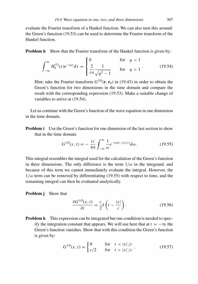
19.4 Wave equation in one, two, and three dimensions 307
evaluate the Fourier transform of a Hankel function. We can also turn this around:the Green’s function (19.53) can be used to determine the Fourier transform of theHankel function.
Problem h Show that the Fourier transform of the Hankel function is given by:
∫ ∞
−∞H (1)
0 (x)e−iqx dx =
⎧
⎪
⎨
⎪
⎩
0 for q < 1
2
iπ
1√
q2 − 1for q > 1
. (19.54)
Hint: take the Fourier transform G2D(r, r0) in (19.43) in order to obtain theGreen’s function for two dimensions in the time domain and compare theresult with the corresponding expression (19.53). Make a suitable change ofvariables to arrive at (19.54).
Let us continue with the Green’s function of the wave equation in one dimensionin the time domain.
Problem i Use the Green’s function for one dimension of the last section to showthat in the time domain
G1D(x, t) = − ic
4π
∫ ∞
−∞
1
ωe−iω(t−|x |/c)dω. (19.55)
This integral resembles the integral used for the calculation of the Green’s functionin three dimensions. The only difference is the term 1/ω in the integrand, andbecause of this term we cannot immediately evaluate the integral. However, the1/ω term can be removed by differentiating (19.55) with respect to time, and theremaining integral can then be evaluated analytically.
Problem j Show that
∂G1D(x, t)
∂t= c
2δ
(
t − |x |c
)
. (19.56)
Problem k This expression can be integrated but one condition is needed to spec-ify the integration constant that appears. We will use here that at t = −∞ theGreen’s function vanishes. Show that with this condition the Green’s functionis given by:
G1D(x, t) =
0 for t < |x | /cc/2 for t > |x | /c
. (19.57)

308 Green’s functions: examples
Just as in two dimensions the solution is nonzero everywhere within the expandingwave front and not only on the wave front |x | = ct as in three dimensions. How-ever, there is an important difference: in two dimensions the solution varies for allmoments with time whereas in one dimension the solution is constant except fort = |x | /c. The human ear is only sensitive to pressure variations, it is insensitiveto a static pressure. Therefore a one-dimensional human will only hear a sound att = |x | /c but not at later times.
In order to appreciate the difference in sound propagation in one, two, and threespace dimensions, the Green’s functions for the different dimensions are sketchedin Figure 19.3. Note the dramatic change in the response for different numbers ofdimensions. This change in the properties of the Green’s function with change indimension has been used somewhat jokingly by Morley [71] to give “a simple proofthat the world is three dimensional.” When you worked through Sections 19.1 and19.2 you learned that for both the heat equation and the Schrodinger equation thesolution does not depend fundamentally on the number of dimensions. This is instark contrast with the solutions of the wave equation which depend critically onthe number of dimensions.
19.5 If I can hear you, you can hear me
In this section we treat a property of the Green’s function of acoustic waves. Westart with the acoustic wave equation:
∇ ·(
1
ρ(r)∇ p
)
+ ω2
κ(r)p = f . (8.7)
The density ρ(r) and the bulk modulus κ(r) can be arbitrary functions of position.Let a solution p1 be excited by an excitation f1 and a solution p2 by an excitation f2.As shown in Section 8.3 the two solutions are related by the following expression
∮
S
1
ρ(p2∇ p1 − p1∇ p2) · dS =
∫
Vp2 f1 − p1 f2 dV . (8.11)
Let us consider a volume V that is either bounded by a free surface where p = 0,or that extends to infinity. The parts of the boundary that form a free surface do notcontribute to the surface integral in the left-hand side, because at the free surfacep = 0, so that the integrand vanishes.
Problem a At the parts of the surface S that are placed at infinity, the radiationboundary condition (19.35) applies. Show that with this boundary condition

19.5 If I can hear you, you can hear me 309
p = 0
r2r1
p = 0
r2r1
Fig. 19.4 Paths that connect the points r1 and r2 in opposite directions. The wavesthat propagate in the two opposite directions are identical.
the contributions of the surface S to the integral in the left-hand side of (8.11)vanishes.
This means that for the volume under consideration the left-hand side of (8.11)vanishes. This result holds for a general excitation f1,2. Let us take f1(r) =δ(r − r1), a point source at location r1. The response to this excitation is the Green’sfunction: p1(r) = G(r, r1). Similarly, we take for the excitation of p2 a delta func-tion placed at location r2, so that f2(r) = δ(r − r2). The corresponding pressurefield is given by the Green’s function p2(r) = G(r, r2).
Problem b Insert these solutions into equation (8.11), use that the left-hand sidevanishes, and show that
G(r1, r2) = G(r2, r1). (19.58)
This result is called the reciprocity theorem. The Green’s function G(r1, r2)gives the pressure at location r1 due to a point source at r2, while the Green’sfunction G(r2, r1) gives the pressure at location r2 due to a point source at r1.According to expression (19.58) these solutions are identical. This means that therole of the source and receiver can be interchanged, and the recorded pressure fieldis identical. This situation is sketched in Figure 19.4. Note that the density and bulkmodulus can be arbitrary functions of space. This means that the waves may travelalong a multitude of paths. Since we allowed for the presence of a free surface,the pressure waves may also bounce off the free surface. Intuitively, it is clear thatthe travel time from r1 to r2 is the same as the travel time from r2 to r1. However, thereciprocity theorem (19.58) states that this holds for the amplitude as well, and thatthe complete waveforms are identical.
This means that if I can hear you, you can hear me, regardless of how complex themedium is, and how many many echoes it may produce. (Provided that our sense ofhearing is equally good.) This also implies that if one submarine can detect another

310 Green’s functions: examples
submarine with its sonar, then the second submarine can detect the first one as well.(Assuming that their sonar equipment is equally sensitive.) This property holds nomatter how complex the distribution of the speed of sound in the ocean may be. Thereciprocity theorem does not hold only for acoustic waves. Elastic waves satisfy asimilar reciprocity theorem that incorporates the vector character of elastic waves[3, 43]. Reciprocity holds as well for the solutions of the heat equation (19.1) nomatter what the spatial distribution of the conductivity κ(r) is.

20
Normal modes
Many physical systems have the property that they can carry out oscillations atcertain specific frequencies only. As a child (and hopefully also as an adult) youwill have discovered that a swing in a playground will move only with a specificnatural period, and that the force that pushes the swing is only effective when theperiod of the force matches the period of the swing. The patterns of motion at whicha system oscillates are called the normal modes of the system. A swing has onenormal mode, but you have seen in Section 13.6 that a simple model of a tri-atomicmolecule has three normal modes. An example of a normal mode of a system isgiven in Figure 20.1 which shows the pattern of oscillation of a metal plate whichis driven by an oscillator at a fixed frequency. The screw in the middle of the plateshows the point at which the force on the plate is applied. Sand is sprinkled on theplate. When the frequency of the external force is equal to the frequency of a normalmode of the plate, the motion of the plate is given by the motion that correspondsto that specific normal mode. Such a pattern of oscillation has nodal lines wherethe motion vanishes. These nodal lines are visible because the sand on the platecollects at these lines.
In this chapter, the normal modes of a variety of systems are analyzed. Normalmodes play an important role in a variety of applications because the eigenfrequen-cies of normal modes provide important information of physical systems. Examplesinclude the spectral lines of light emitted by atoms which have led to the advent ofquantum mechanics and its description of the structure of atoms, and the normalmodes of the Earth which provide information about the structure of our planet.In addition, normal modes are used in this chapter to introduce some properties ofspecial functions, such as Bessel functions and Legendre functions. This is achievedby analyzing the normal modes of a system in one, two, and three dimensions inSections 20.1–20.3.
311
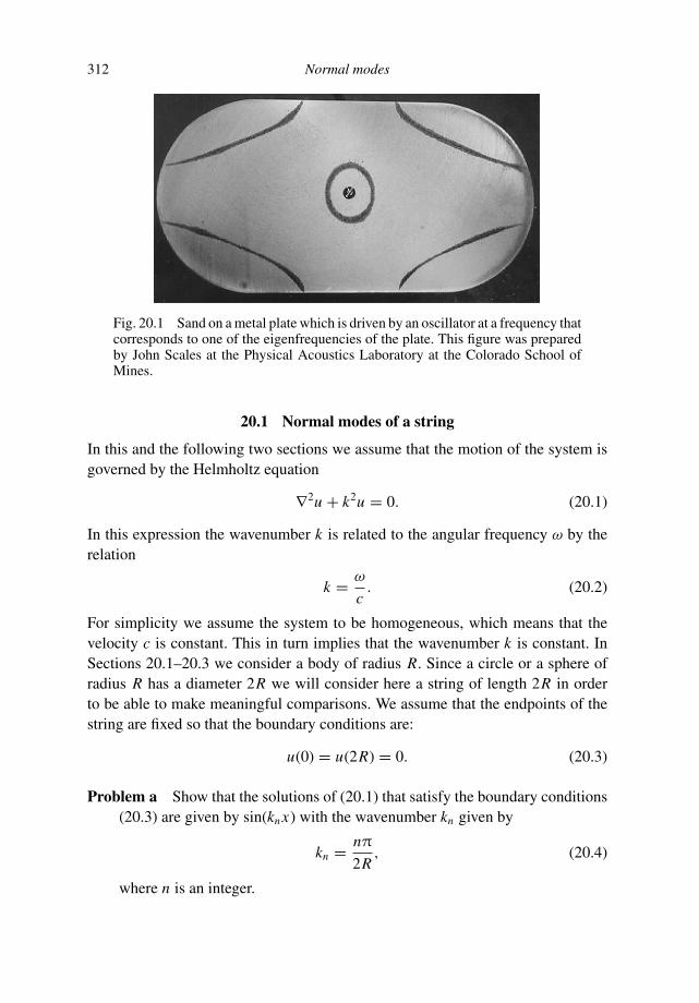
312 Normal modes
Fig. 20.1 Sand on a metal plate which is driven by an oscillator at a frequency thatcorresponds to one of the eigenfrequencies of the plate. This figure was preparedby John Scales at the Physical Acoustics Laboratory at the Colorado School ofMines.
20.1 Normal modes of a string
In this and the following two sections we assume that the motion of the system isgoverned by the Helmholtz equation
∇2u + k2u = 0. (20.1)
In this expression the wavenumber k is related to the angular frequency ω by therelation
k = ω
c. (20.2)
For simplicity we assume the system to be homogeneous, which means that thevelocity c is constant. This in turn implies that the wavenumber k is constant. InSections 20.1–20.3 we consider a body of radius R. Since a circle or a sphere ofradius R has a diameter 2R we will consider here a string of length 2R in orderto be able to make meaningful comparisons. We assume that the endpoints of thestring are fixed so that the boundary conditions are:
u(0) = u(2R) = 0. (20.3)
Problem a Show that the solutions of (20.1) that satisfy the boundary conditions(20.3) are given by sin(knx) with the wavenumber kn given by
kn = nπ
2R, (20.4)
where n is an integer.
20.1 Normal modes of a string 313
For a number of purposes it is useful to normalize the modes: this means that werequire that the modes un(x) satisfy the condition
∫ 2R0 u2
n(x)dx = 1.
Problem b Show that the normalized modes are given by
un(x) = 1√R
sin(knx). (20.5)
Problem c Sketch the modes for several values of n as a function of the distancex .
Problem d The modes un(x) are orthogonal, which means that the inner product∫ 2R
0 un(x)um(x)dx vanishes when n = m. Give a proof of this property byderiving that
∫ 2R
0un(x)um(x)dx = δnm . (20.6)
We conclude from this section that the modes of a string are oscillatory functionswith a wavenumber that can only have discrete well-defined values kn . Accordingto (20.2) this means that the string can only vibrate at discrete frequencies whichare given by
ωn = nπc
2R. (20.7)
This property may be familiar to you because you probably know that a guitar stringvibrates only at very specific frequencies which determine the pitch of the soundthat you hear. The results of this section imply that each string oscillates not onlyat one particular frequency, but at many discrete frequencies. The oscillation withthe lowest frequency is given by (20.7) with n = 1: this is called the fundamentalmode or ground-tone. This is what the ear perceives as the pitch of the tone. Theoscillations corresponding to larger values of n are called the higher modes orovertones. The particular mix of overtones determines the timbre of the signal.If the higher modes are strongly excited the ear perceives this sound as metallic,whereas just the fundamental mode is perceived as a smooth sound. The readerwho is interested in the theory of musical instruments can consult reference [88].
The discrete modes are not a peculiarity of the string. Most systems that supportwaves and that are of a finite extent support modes. For example, in Figure 15.1the spectrum of the sound of a soprano saxophone is shown. This spectrum ischaracterized by well-defined peaks that correspond to the modes of the air-wavesin the instrument. Mechanical systems in general have discrete modes, these modescan be destructive when they are excited at their resonance frequency. The matter

314 Normal modes
waves in atoms are organized in modes as well, and this is ultimately the reasonwhy atoms in an excited state emit light only at very specific frequencies, calledspectral lines.
20.2 Normal modes of a drum
In the previous section we looked at the modes of a one-dimensional system. Herewe derive the modes of a two-dimensional system which is a model of a drum. Weconsider a two-dimensional membrane that satisfies the Helmholtz equation (20.1).The membrane is circular and has radius R. At the edge r = R the membranecannot move, this means that in cylindrical coordinates the boundary condition forthe waves u(r, ϕ) is given by:
u(R, ϕ) = 0. (20.8)
In order to find the modes of the drum we will use separation of variables, whichmeans that we seek solutions that can be written as a product of a function thatdepends only on r and a function that depends only on ϕ:
u(r, ϕ) = F(r )G(ϕ). (20.9)
Problem a Insert this solution into the Helmholtz equation, use the expression ofthe Laplacian in cylindrical coordinates, and show that the resulting equationcan be written as
[
1
F(r )r
∂
∂r
(
r∂ F
∂r
)
+ k2r2
]
︸ ︷︷ ︸
(A)
= − 1
G(ϕ)
∂2G
∂ϕ2︸ ︷︷ ︸
(B)
. (20.10)
Problem b The terms labeled (A) depend only on the variable r whereas the termslabeled (B) depend only on the variable ϕ. These terms can only be equal forall values of r and ϕ when they depend neither on r nor on ϕ, that is whenthey are a constant. Use this to show that F(r ) and G(ϕ) satisfy the followingdifferential equations:
d2 F
dr2+ 1
r
d F
dr+(
k2 − µ
r2
)
F = 0, (20.11)
d2G
dϕ2+ µG = 0, (20.12)
where µ is a constant that is not yet known.
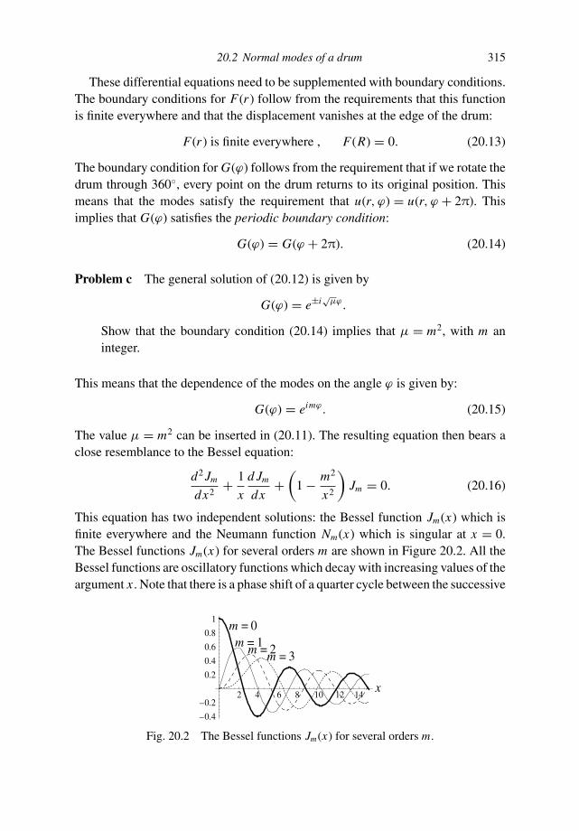
20.2 Normal modes of a drum 315
These differential equations need to be supplemented with boundary conditions.The boundary conditions for F(r ) follow from the requirements that this functionis finite everywhere and that the displacement vanishes at the edge of the drum:
F(r ) is finite everywhere , F(R) = 0. (20.13)
The boundary condition for G(ϕ) follows from the requirement that if we rotate thedrum through 360, every point on the drum returns to its original position. Thismeans that the modes satisfy the requirement that u(r, ϕ) = u(r, ϕ + 2π). Thisimplies that G(ϕ) satisfies the periodic boundary condition:
G(ϕ) = G(ϕ + 2π). (20.14)
Problem c The general solution of (20.12) is given by
G(ϕ) = e±i√
µϕ.
Show that the boundary condition (20.14) implies that µ = m2, with m aninteger.
This means that the dependence of the modes on the angle ϕ is given by:
G(ϕ) = eimϕ. (20.15)
The value µ = m2 can be inserted in (20.11). The resulting equation then bears aclose resemblance to the Bessel equation:
d2 Jm
dx2+ 1
x
d Jm
dx+(
1 − m2
x2
)
Jm = 0. (20.16)
This equation has two independent solutions: the Bessel function Jm(x) which isfinite everywhere and the Neumann function Nm(x) which is singular at x = 0.The Bessel functions Jm(x) for several orders m are shown in Figure 20.2. All theBessel functions are oscillatory functions which decay with increasing values of theargument x . Note that there is a phase shift of a quarter cycle between the successive
2 4 6 8 10 12 14x
–0.4
–0.2
0.2
0.4
0.6
0.8
1m = 0m = 1m = 2m = 3
Fig. 20.2 The Bessel functions Jm(x) for several orders m.
316 Normal modes
orders m. Near x = 0 the lowest order Bessel functions behave as J0(x) ∼ 1, whilethe higher order Bessel functions behave as J1(x) ∼ x and J2(x) ∼ x2. This is dueto the fact that the Bessel function Jm(x) behaves as xm for small values of x .
Problem d Show that the general solution of (20.11) can be written as:
F(r ) = AJm(kr ) + B Nm(kr ), (20.17)
with A and B integration constants.
Problem e Use the boundary conditions of F(r ) to show that B = 0 and that thewavenumber k must take a value such that Jm(k R) = 0.
This last condition for the wavenumber is analogous to the condition (20.4) for theone-dimensional string. For both the string and the drum the wavenumber can onlytake discrete values: these values are dictated by the condition that the displacementvanishes at the outer boundary of the string or the drum. For the drum there are forevery value of the angular degree m infinitely many wavenumbers that satisfy therequirement Jm(k R) = 0. These wavenumbers are labeled with a subscript n, butsince these wavenumbers are different for each value of the angular order m, theallowed wavenumbers carry two indices and are denoted here by k(m)
n . They satisfythe condition
Jm(k(m)n R) = 0. (20.18)
The zeroes (or roots) of the Bessel function Jm(x) are not known in closed analyticalform. However, numerical tables exists for the roots of Bessel functions, see for ex-ample, Table 9.4 of Abramowitz and Stegun [1]. Take a look at this reference whichcontains a bewildering collection of formulas, graphs, and tables of mathematicalfunctions. The lowest order zeroes of the Bessel functions J0(x), J1(x), . . . , J5(x)are shown in Table 20.1.
Using the results in this section it follows that the modes of the drum are givenby
unm(r, ϕ) = Jm(k(m)n r )eimϕ. (20.19)
Problem f Let us first consider the ϕ-dependence of these modes. Show that whenone follows the mode unm(r, ϕ) along a complete circle around the origin oneencounters exactly m oscillations of that mode.
Problem g Find the eigenfrequencies of the five modes of the drum with thelowest frequencies and make a sketch of the associated standing waves of the
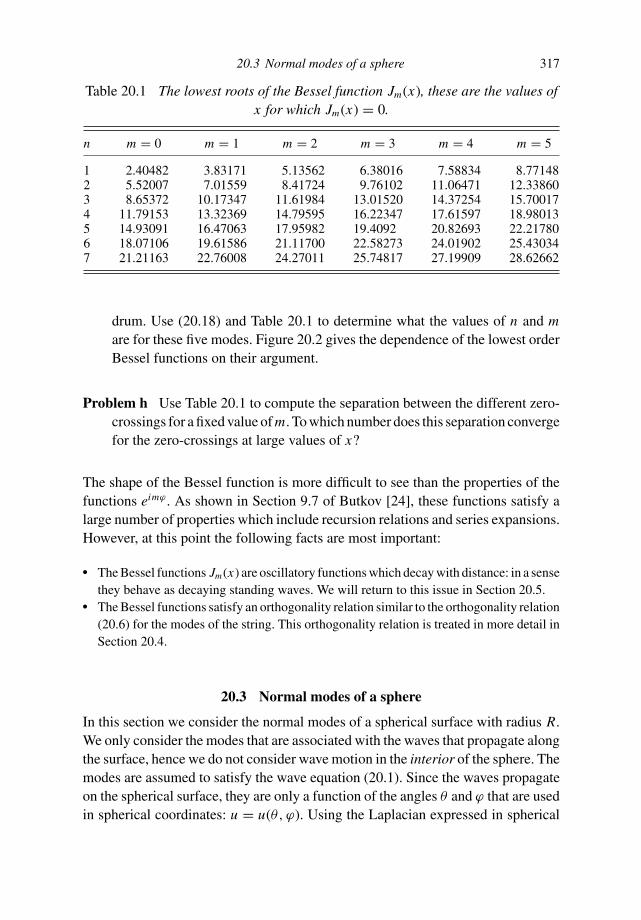
20.3 Normal modes of a sphere 317
Table 20.1 The lowest roots of the Bessel function Jm(x), these are the values ofx for which Jm(x) = 0.
n m = 0 m = 1 m = 2 m = 3 m = 4 m = 5
1 2.40482 3.83171 5.13562 6.38016 7.58834 8.771482 5.52007 7.01559 8.41724 9.76102 11.06471 12.338603 8.65372 10.17347 11.61984 13.01520 14.37254 15.700174 11.79153 13.32369 14.79595 16.22347 17.61597 18.980135 14.93091 16.47063 17.95982 19.4092 20.82693 22.217806 18.07106 19.61586 21.11700 22.58273 24.01902 25.430347 21.21163 22.76008 24.27011 25.74817 27.19909 28.62662
drum. Use (20.18) and Table 20.1 to determine what the values of n and mare for these five modes. Figure 20.2 gives the dependence of the lowest orderBessel functions on their argument.
Problem h Use Table 20.1 to compute the separation between the different zero-crossings for a fixed value of m. To which number does this separation convergefor the zero-crossings at large values of x?
The shape of the Bessel function is more difficult to see than the properties of thefunctions eimϕ . As shown in Section 9.7 of Butkov [24], these functions satisfy alarge number of properties which include recursion relations and series expansions.However, at this point the following facts are most important:
The Bessel functions Jm(x) are oscillatory functions which decay with distance: in a sensethey behave as decaying standing waves. We will return to this issue in Section 20.5.
The Bessel functions satisfy an orthogonality relation similar to the orthogonality relation(20.6) for the modes of the string. This orthogonality relation is treated in more detail inSection 20.4.
20.3 Normal modes of a sphere
In this section we consider the normal modes of a spherical surface with radius R.We only consider the modes that are associated with the waves that propagate alongthe surface, hence we do not consider wave motion in the interior of the sphere. Themodes are assumed to satisfy the wave equation (20.1). Since the waves propagateon the spherical surface, they are only a function of the angles θ and ϕ that are usedin spherical coordinates: u = u(θ, ϕ). Using the Laplacian expressed in spherical
318 Normal modes
coordinates, wave equation (20.1) is then given by
1
R2
[
1
sin θ
∂
∂θ
(
sin θ∂u
∂θ
)
+ 1
sin2 θ
∂2u
∂ϕ2
]
+ k2u = 0. (20.20)
Again, we seek a solution by applying separation of variables by writing the solutionin a form similar to (20.9):
u(θ, ϕ) = F(θ )G(ϕ). (20.21)
Problem a Insert this into (20.20) and apply separation of variables to show thatF(θ ) satisfies the following differential equation:
sin θd
dθ
(
sin θd F
dθ
)
+ (k2 R2 sin2 θ − µ)
F = 0, (20.22)
and that G(ϕ) satisfies (20.12), where the unknown constant µ does not dependon θ or ϕ.
To make further progress we have to apply boundary conditions. Just as with thedrum in Section 20.2, the system is invariant when a rotation over 2π is applied:u(θ, ϕ) = u(θ, ϕ + 2π). This means that G(ϕ) satisfies the same differential equa-tion (20.12) as for the case of the drum and the same periodic boundary condition(20.14). The solution is therefore given by G(ϕ) = eimϕ and the separation constantsatisfies µ = m2, with m an integer. Using this, the differential equation for F(θ )can be written as:
1
sin θ
d
dθ
(
sin θd F
dθ
)
+(
k2 R2 − m2
sin2 θ
)
F = 0. (20.23)
Before we continue let us compare this equation with (20.11) for the modes of thedrum which we can rewrite as
1
r
d
dr
(
rd F
dr
)
+(
k2 − m2
r2
)
F = 0. (20.11)
Note that these equations are identical when we compare r in (20.11) with sin θ
in (20.23). There is a good reason for this. Suppose that we have a source in themiddle of the drum. Then the variable r measures the distance from a point on thedrum to the source. This can be compared with the case of waves on a sphericalsurface that are excited by a source at the north pole. In that case, sin θ is a measureof the distance from a point to the source point. The only difference is that sin θ
enters the equation rather than the true angular distance θ . This is a consequence
20.3 Normal modes of a sphere 319
of the fact that the surface is curved, and this curvature leaves an imprint on thedifferential equation that the modes satisfy.
Problem b The differential equation (20.11) was reduced in Section 20.2 to theBessel equation by changing to a new variable x = kr . Define a new variable
x ≡ cos θ (20.24)
and show that the differential equation (20.23) is given by
d
dx
[
(
1 − x2) d F
dx
]
+(
k2 R2 − m2
1 − x2
)
F = 0. (20.25)
The solution of this differential equation is given by the associated Legendrefunctions Pm
l (x). These functions are described in great detail in Section 9.8 ofButkov [24]. In fact, just like the Bessel equation, the differential equation (20.25)has a solution that is regular as well as a solution Qm
l (x) that is singular at the pointx = 1 where θ = 0. However, since the modes are finite everywhere, they are givenonly by the regular solution Pm
l (x).The wavenumber k is related to frequency by the relation k = ω/c. At this point
it is not clear what k is, hence the eigenfrequencies of the spherical surface are notyet known. It is shown in Section 9.8 of Butkov [24] that:
The associated Legendre functions are only finite when the wavenumber satisfies
k2 R2 = l(l + 1), (20.26)
where l is a positive integer. Using this in (20.25) implies that the associated Legendrefunctions satisfy the following differential equation:
1
sin θ
d
dθ
[
sin θd Pm
l (cos θ )
dθ
]
+[
l (l + 1) − m2
sin2 θ
]
Pml (cos θ ) = 0.
(20.27)
Seen as a function of x (= cos θ ) this is equivalent to the following differential equation
d
dx
[
(
1 − x2) d Pml (x)
dx
]
+[
l (l + 1) − m2
1 − x2
]
Pml (x) = 0.
The integer l must be larger than or equal to the absolute value of the angular order m.
Problem c Show that the last condition can also be written as:
−l ≤ m ≤ l. (20.28)
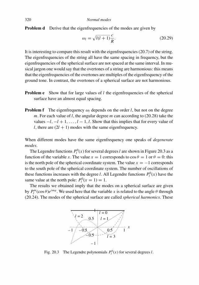
320 Normal modes
Problem d Derive that the eigenfrequencies of the modes are given by
ωl =√
l(l + 1)c
R. (20.29)
It is interesting to compare this result with the eigenfrequencies (20.7) of the string.The eigenfrequencies of the string all have the same spacing in frequency, but theeigenfrequencies of the spherical surface are not spaced at the same interval. In mu-sical jargon one would say that the overtones of a string are harmonious: this meansthat the eigenfrequencies of the overtones are multiples of the eigenfrequency of theground tone. In contrast, the overtones of a spherical surface are not harmonious.
Problem e Show that for large values of l the eigenfrequencies of the sphericalsurface have an almost equal spacing.
Problem f The eigenfrequency ωl depends on the order l, but not on the degreem. For each value of l, the angular degree m can according to (20.28) take thevalues −l, −l + 1, . . . , l − 1, l. Show that this implies that for every value ofl, there are (2l + 1) modes with the same eigenfrequency.
When different modes have the same eigenfrequency one speaks of degeneratemodes.
The Legendre functions P0l (x) for several degrees l are shown in Figure 20.3 as a
function of the variable x . The value x = 1 corresponds to cos θ = 1 or θ = 0: thisis the north pole of the spherical coordinate system. The value x = −1 correspondsto the south pole of the spherical coordinate system. The number of oscillations ofthese functions increases with the degree l. All Legendre functions P0
l (x) have thesame value at the north pole: P0
l (x = 1) = 1.The results we obtained imply that the modes on a spherical surface are given
by Pml (cos θ )eimϕ . We used here that the variable x is related to the angle θ through
(20.24). The modes of the spherical surface are called spherical harmonics. These
– 1 – 0.5 0.5 1x
– 1
– 0.5
0.5
1l = 0
l = 1l = 2
l = 3
Fig. 20.3 The Legendre polynomials P0l (x) for several degrees l.

20.3 Normal modes of a sphere 321
eigenfunctions for m ≥ 0 are given by:
Ylm(θ, ϕ) = (−1)m
√
2l + 1
4π
(l − m)!
(l + m)!Pm
l (cos θ )eimϕ m ≥ 0. (20.30)
For m < 0 the spherical harmonics are defined by the relation
Ylm(θ, ϕ) = (−1)m Yl,−m(θ, ϕ). (20.31)
You may wonder where the square-root in front of the associated Legendre functioncomes from. One can show that with this numerical factor the spherical harmonicsare normalized when integrated over the sphere:
∫∫
|Ylm |2 dΩ = 1, (20.32)
where∫∫ · · · dΩ denotes an integration over the unit sphere. You should be
aware of the fact that different authors use different definitions of the spheri-cal harmonics. For example, one could also define the spherical harmonics asYlm(θ, ϕ) = Pm
l (cos θ )eimϕ because the functions also account for the normalmodes of a spherical surface.
Problem g Show that the modes defined in this way satisfy∫∫ ∣
∣Ylm
∣
∣
2dΩ =
4π/ (2l + 1) × (l + m)!/(l − m)!.
This means that the modes defined in this way are not normalized when integratedover the sphere. There is no reason why one cannot work with this convention, aslong as one accounts for the fact that in this definition the modes are not normalized.Throughout this book we will use the definition (20.30) for the spherical harmonics.In doing so we follow the normalization that is used by Edmonds [37].
The real parts of the lowest order spherical harmonics are shown in Figure 20.4,in which these functions are projected on the Earth’s surface. Only those sphericalharmonics with m ≥ 0 are shown, the spherical harmonics for m < 0 follow from(20.31). Just as with the Bessel functions, the associated Legendre functions satisfyrecursion relations and a large number of other properties which are described indetail in Section 9.8 of Butkov [24]. The most important properties of the sphericalharmonics Ylm(θ, ϕ) are:
These functions display m oscillations when the angle ϕ increases by 2π. In other words,there are m oscillations along one circle of constant latitude.
The associated Legendre functions Pml (cos θ ) behave like Bessel functions in the sense
that they behave like standing waves with an amplitude that decays from the pole. Wereturn to this issue in Section 20.6.

322 Normal modes
Fig. 20.4 The real parts of the lowest order spherical harmonics. The value ofthe order l and degree m is shown above each panel. Negative values are shown inwhite, positive values in black. Each panel shows the surface of the complete sphereusing a Hammer projection. The world map is shown to provide spatial orientation.The thin solid lines correspond to lines of constant latitude and longitude on thesphere. Figure courtesy of Jeannot Trampert.
The number of oscillations between the north pole of the sphere and the south pole ofthe sphere increases with the difference (l − m).
The spherical harmonics are orthogonal for a suitably chosen inner product; this orthog-onality relation is derived in Section 20.4.
The spherical harmonics are the eigenfunctions of the Laplacian on the sphere.
Problem h Give a proof of this last property by showing that
∇21Ylm(θ, ϕ) = −l (l + 1) Ylm(θ, ϕ), (20.33)
where the Laplacian on the unit sphere is given by
∇21 = 1
sin θ
∂
∂θ
(
sin θ∂
∂θ
)
+ 1
sin2 θ
∂2
∂ϕ2. (20.34)
This property is extremely useful in many applications, because the action of theLaplacian on a sphere can be replaced by the much simpler multiplication by theconstant −l (l + 1) when spherical harmonics are concerned.

20.4 Normal modes of orthogonality relations 323
20.4 Normal modes of orthogonality relations
The normal modes of a physical system often satisfy orthogonality relations whena suitably chosen inner product for the eigenfunctions is used. In this section thisis illustrated by studying once again the normal modes of the Helmholtz equation(20.1) for different geometries. In this section we derive first the general orthogo-nality relation for these normal modes. This is then applied to the normal modes ofthe previous sections to derive the orthogonality relations for Bessel functions andassociated Legendre functions.
Let us consider two normal modes of the Helmholtz equation (20.1), and letthese modes be called u p and uq . At this point we leave it open whether the modesare defined on a line, on a surface of arbitrary shape or in a volume. The inte-gration over the region of space in which the modes are defined is denoted as∫ · · · d N x , where N is the dimension of this space. The wavenumbers of thesemodes, which are effectively the corresponding eigenvalues of the Helmholtz equa-tion, are defined by kp and kq , respectively. In other words, the modes satisfy theequations:
∇2u p + k2pu p = 0, (20.35)
∇2uq + k2quq = 0. (20.36)
The subscript p may stand for a single mode index such as in the index n forthe wavenumber kn for the modes of a string, or it may stand for a number ofindices such as the indices nm that label the eigenfunctions (20.19) of a circulardrum.
Problem a Multiply (20.35) by u∗q , take the complex conjugate of (20.36) and
multiply the result by u p. Subtract the resulting equations and integrate thisover the region of space for which the modes are defined to show that
∫
(
u∗q∇2u p − u p∇2u∗
q
)
d N x + (k2p − k∗2
q
)
∫
u∗qu pd N x = 0. (20.37)
Problem b Use the theorem of Gauss to derive that∫
u∗q∇2u pd N x =
∮
u∗q∇u p · dS −
∫
(∇u∗q · ∇u p
)
d N x, (20.38)
where the integral∮ · · · dS is over the surface that bounds the body. If you
have trouble deriving this, you can consult (8.10) where a similar result wasused for the derivation of the representation theorem for acoustic waves.

324 Normal modes
Problem c Use the last result to show that expression (20.37) can be written as∮
(
u∗q∇u p − u p∇u∗
q
) · dS + (k2p − k∗2
q
)
∫
u∗qu pd N x = 0. (20.39)
Problem d The first term is an integral over the boundary of the body. The secondterm contains a volume integral and this term leads to the orthogonality relationof the modes. Let us assume that on this boundary the modes satisfy one ofthe three boundary conditions: (i) u = 0, (ii) n · ∇u = 0 (where n is the unitvector perpendicular to the surface) or (iii) n · ∇u = αu (whereα is a constant).Show that for all of these boundary conditions the surface integral in (20.39)vanishes.
The last result implies that when the modes satisfy one of these boundary conditions
(
k2p − k∗2
q
)
∫
u∗qu pd N x = 0. (20.40)
Let us first consider the case in which the modes are equal, that is in which p = q.In that case the integral reduces to
∫ ∣
∣u p
∣
∣
2d N x which is guaranteed to be positive.
Equation (20.40) then implies that k2p = k∗2
p , so that the wavenumbers kp must bereal: kp = k∗
p . For this reason the complex conjugate of the wavenumbers can bedropped and (20.40) can be written as:
(
k2p − k2
q
)
∫
u∗qu pd N x = 0. (20.41)
Now consider the case of two different modes for which the wavenumbers kp andkq are different. In that case the term
(
k2p − k2
q
)
is nonzero, hence in order to satisfy(20.41) the modes must satisfy
∫
u∗qu pd N x = 0 for kp = kq . (20.42)
This finally gives the orthogonality relation of the modes in the sense that itstates that the modes are orthogonal for the following inner product: 〈 f · g〉 ≡∫
f ∗g d N x . Note that the inner product for which the modes are orthogonal fol-lows from the Helmholtz equation (20.1) which defines the modes.
Let us now consider this orthogonality relation for the modes of the string,the drum, and the spherical surface of the previous sections. For the string, theorthogonality relation was derived in problem d of Section 20.1 and you can seethat equation (20.6) is identical to the general orthogonality relation (20.42). Forthe circular drum the modes are given by (20.19).

20.4 Normal modes of orthogonality relations 325
Problem e Use (20.19) for the modes of the circular drum to show that the or-thogonality relation (20.42) for this case can be written as:
∫ R
0
∫ 2π
0Jm1 (k
(m1)n1
r )Jm2 (k(m2)n2
r )ei(m1−m2)ϕdϕ rdr
= 0 for k(m1)n1
= k(m2)n2
. (20.43)
Explain where the factor r comes from in the integration.
Problem f This integral can be separated into an integral over ϕ and an integralover r . The ϕ-integral is given by
∫ 2π0 ei(m1−m2)ϕdϕ. Show that this integral
vanishes when m1 = m2:∫ 2π
0ei(m1−m2)ϕdϕ = 0 for m1 = m2. (20.44)
Note that you obtained this relation earlier in (17.9) in the derivation of theresidue theorem.
Expression (20.44) implies that the modes un1m1 (r, ϕ) and un2m2 (r, ϕ) are orthog-onal when m1 = m2 because the ϕ-integral in (20.43) vanishes when m1 = m2. Letus now consider why the different modes of the drum are orthogonal when m1 andm2 are equal to the same integer m. In that case (20.43) implies that
∫ R
0Jm(k(m)
n1r )Jm(k(m)
n2r ) r dr = 0 for n1 = n2. (20.45)
Note that we have used here that k(m)n1
= k(m)n2
when n1 = n2. This integral definesan orthogonality relation for Bessel functions. Note that both Bessel functions inthis relation are of the same degree m but that the wavenumbers in the argument ofthe Bessel functions differ. Note the resemblance between this expression and theorthogonality relation (20.6) of the modes of the string which can be written as
∫ 2R
0sin(knx) sin(km x) dx = 0 for n = m. (20.46)
The presence of the term r in the integral (20.45) comes from the fact that the modesof the drum are orthogonal for the integration over the total area of the drum. Incylindrical coordinates this leads to a factor r in the integration.
Problem g Take your favorite book on mathematical physics and find an alterna-tive derivation of the orthogonality relation (20.45) of the Bessel functions ofthe same degree m.

326 Normal modes
Note finally that the modes un1m1 (r, ϕ) and un2m2 (r, ϕ) are orthogonal when m1 = m2
because the ϕ-integral satisfies (20.44), whereas the modes are orthogonal whenn1 = n2 but with the same order m because the r -integral (20.45) vanishes in thatcase. This implies that the eigenfunctions of the drum defined in (20.19) satisfy thefollowing orthogonality relation:
∫ R
0
∫ 2π
0u∗
n1m1(r, ϕ)un2m2 (r, ϕ) dϕ rdr = Cδn1n2δm1m2, (20.47)
where δi j is the Kronecker delta and C is a constant that depends on n1 and m1.A similar analysis can be applied to the spherical harmonics Ylm(θ, ϕ) which
are the eigenfunctions of the Helmholtz equation on a spherical surface. You maywonder in that case what the boundary conditions of these eigenfunctions are be-cause in the step from (20.39) to (20.40) the boundary conditions of the modeshave been used. A closed surface, however, has no boundary. This means that thesurface integral in (20.39) vanishes. This in turn means that the orthogonality rela-tion (20.42) holds despite the fact that the spherical harmonics do not satisfy one ofthe boundary conditions that was used in problem d. Let us now consider the innerproduct of two spherical harmonics on the sphere:
∫∫
Y ∗l1m1
(θ, ϕ)Yl2m2 (θ, ϕ)dΩ.
Problem h Show that the ϕ-integral in the integration over the sphere is of theform
∫ 2π0 ei(m2−m1)dϕ and that this integral is equal to 2πδm1m2 .
This implies that the spherical harmonics are orthogonal when m1 = m2 becauseof the ϕ-integration. We will now continue with the case in which m1 = m2, anddenote this common value with the single index m.
Problem i Use the general orthogonality relation (20.42) to derive that the asso-ciated Legendre functions satisfy the following orthogonality relation:
∫ π
0Pm
l1(cos θ )Pm
l2(cos θ ) sin θdθ = 0 when l1 = l2. (20.48)
Note the common value of the degree m in the two associated Legendre func-tions. Also show explicitly that the condition kl1 = kl2 is equivalent to thecondition l1 = l2.
Problem j Use a substitution of variables to show that this orthogonality relationcan also be written as
∫ 1
−1Pm
l1(x)Pm
l2(x)dx = 0 when l1 = l2. (20.49)
20.5 Bessel functions behave as decaying cosines 327
Problem k Find an alternative derivation of this orthogonality relation in theliterature.
The result you obtained in problem h implies that the spherical harmonics areorthogonal when m1 = m2 because of the ϕ-integration, whereas problem i im-plies that the spherical harmonics are orthogonal when l1 = l2 because of theθ -integration. This means that the spherical harmonics satisfy the following or-thogonality relation:
∫∫
Y ∗l1m1
(θ, ϕ)Yl2m2 (θ, ϕ) dΩ = δl1l2δm1m2 . (20.50)
The numerical constant multiplying the delta functions is equal to 1. This is aconsequence of the square-root term in (20.30) that pre-multiplies the associatedLegendre functions. Be aware of the fact that when a different convention is usedfor the normalization of the spherical harmonics a normalization factor appears onthe right-hand side of the orthogonality relation (20.50) of the spherical harmonics.
20.5 Bessel functions behave as decaying cosines
As we have seen in Section 20.2 the modes of the circular drum are given byJm(kr )eimϕ , where the Bessel function satisfies the differential equation (20.16) andwhere k is a wavenumber chosen in such a way that the displacement at the edge ofthe drum vanishes. We show in this section that the waves that propagate through thedrum have an approximately constant wavelength, but that their amplitude decayswith the distance to the center of the drum. The starting point of the analysis is theBessel equation
d2 Jm
dx2+ 1
x
d Jm
dx+(
1 − m2
x2
)
Jm = 0. (20.16)
If the terms (1/x)d Jm/dx and m2/x2 were absent in (20.16) the Bessel equationwould reduce to the differential equation d2 F/dx2 + F = 0 whose solutions aregiven by a superposition of cos x and sin x . We can therefore expect the Besselfunctions to display an oscillatory behavior when x is large.
It follows directly from (20.16) that the term m2/x2 is relatively small for largevalues of x , specifically when x m. However, it is not obvious under whichconditions the term (1/x)d Jm/dx is relatively small. Fortunately this term can betransformed away.
Problem a Write Jm(x) = xαgm(x), insert this in the Bessel equation (20.16),and show that the term with the first derivative vanishes when α = −1/2 and

328 Normal modes
that the resulting differential equation for gm(x) is given by
d2gm
dx2+(
1 − m2 − 1/4
x2
)
gm = 0. (20.51)
Up to this point we have made no approximations. Although we have transformedthe first derivative term out of the Bessel equation, we still cannot solve (20.51).However, when x m the term proportional to 1/x2 in this expression is rela-tively small. This means that for large values of x the function gm(x) satisfies theapproximate differential equation d2gm/dx2 + gm ≈ 0.
Problem b Show that the solution of this equation is given by gm(x) ≈A cos (x + ϕ), where A and ϕ are constants. Also show that this implies thatthe Bessel function is approximately given by:
Jm(x) ≈ Acos (x + ϕ)√
x. (20.52)
This approximation is obtained from a local analysis of the Bessel equation. Sinceall values of the constants A and ϕ lead to a solution that approximately satisfies thedifferential equation (20.51), it is not possible to retrieve the precise values of theseconstants from the analysis in this section. An analysis based on the asymptoticevaluation of the integral representation of the Bessel function as presented inSection 24.5 or reference [14] shows that:
Jm(x) =√
2
πxcos[
x − (2m + 1)π
4
]
+ O(x−3/2). (20.53)
Problem c As a check on the accuracy of this asymptotic expression let us com-pare the zeroes of this approximation with the zeroes of the Bessel functions asgiven in Table 20.1. In problem h of Section 20.2 you found that the separationof the zero-crossings tends to π for large values of x . Explain this using theapproximate expression (20.53). How large must x be for the different valuesof the degree m so that the difference in the spacing of the zero-crossings withπ is less than 0.01?
The asymptotic expression (20.53) can be compared in Figure 20.5 with theBessel functions Jm(x) for the degrees m = 0 and m = 2, respectively. For largevalues of x , the approximation (20.53) is very good. Note that for m = 0 theapproximation is better for smaller values of x than it is for m = 2. This isrelated to the fact that the approximation (20.53) is valid under the condition
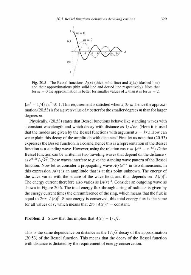
20.5 Bessel functions behave as decaying cosines 329
2 4 6 8 10 12 14x
–1
–0.5
0.5
1 m = 0
m = 2
Fig. 20.5 The Bessel functions J0(x) (thick solid line) and J2(x) (dashed line)and their approximations (thin solid line and dotted line respectively). Note thatfor m = 0 the approximation is better for smaller values of x than it is for m = 2.
(
m2 − 1/4)
/x2 1. This requirement is satisfied when x m, hence the approxi-mation (20.53) is for a given value of x better for the smaller degrees m than for largerdegrees m.
Physically, (20.53) states that Bessel functions behave like standing waves witha constant wavelength and which decay with distance as 1/
√kr . (Here it is used
that the modes are given by the Bessel functions with argument x = kr .) How canwe explain this decay of the amplitude with distance? First let us note that (20.53)expresses the Bessel function in a cosine, hence this is a representation of the Besselfunction as a standing wave. However, using the relation cos x = (eix + e−i x
)
/2 theBessel function can be written as two traveling waves that depend on the distance ras e±ikr/
√kr . These waves interfere to give the standing wave pattern of the Bessel
function. Now let us consider a propagating wave A(r )eikr in two dimensions; inthis expression A(r ) is an amplitude that is at this point unknown. The energy ofthe wave varies with the square of the wave field, and thus depends on |A(r )|2.The energy current therefore also varies as |A(r )|2. Consider an outgoing wave asshown in Figure 20.6. The total energy flux through a ring of radius r is given bythe energy current times the circumference of the ring, which means that the flux isequal to 2πr |A(r )|2. Since energy is conserved, this total energy flux is the samefor all values of r , which means that 2πr |A(r )|2 = constant.
Problem d Show that this implies that A(r ) ∼ 1/√
r .
This is the same dependence on distance as the 1/√
x decay of the approximation(20.53) of the Bessel function. This means that the decay of the Bessel functionwith distance is dictated by the requirement of energy conservation.
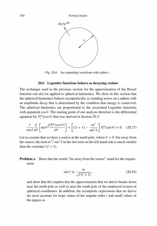
330 Normal modes
A(r)e
r
ikr
Fig. 20.6 An expanding wavefront with radius r .
20.6 Legendre functions behave as decaying cosines
The technique used in the previous section for the approximation of the Besselfunction can also be applied to spherical harmonics. We show in this section thatthe spherical harmonics behave asymptotically as standing waves on a sphere withan amplitude decay that is determined by the condition that energy is conserved.The spherical harmonics are proportional to the associated Legendre functionswith argument cos θ . The starting point of our analysis therefore is the differentialequation for Pm
l (cos θ ) that was derived in Section 20.3:
1
sin θ
d
dθ
[
sin θd Pm
l (cos θ )
dθ
]
+[
l (l + 1) − m2
sin2 θ
]
Pml (cos θ ) = 0. (20.27)
Let us assume that we have a source at the north pole, where θ = 0. Far away fromthe source, the term m2/ sin2 θ in the last term on the left-hand side is much smallerthan the constant l (l + 1).
Problem a Show that the words “far away from the source” stand for the require-ment
sin θ m√l (l + 1)
, (20.54)
and show that this implies that the approximation that we derive breaks downnear the north pole as well as near the south pole of the employed system ofspherical coordinates. In addition, the asymptotic expressions that we deriveare most accurate for large values of the angular order l and small values ofthe degree m.
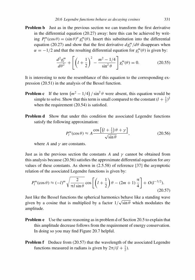
20.6 Legendre functions behave as decaying cosines 331
Problem b Just as in the previous section we can transform the first derivativein the differential equation (20.27) away: here this can be achieved by writ-ing Pm
l (cos θ ) = (sin θ )α gml (θ ). Insert this substitution into the differential
equation (20.27) and show that the first derivative dgml /dθ disappears when
α = −1/2 and that the resulting differential equation for gml (θ ) is given by:
d2gml
dθ2 +[
(
l + 1
2
)2
− m2 − 1/4
sin2 θ
]
gml (θ ) = 0. (20.55)
It is interesting to note the resemblance of this equation to the corresponding ex-pression (20.51) in the analysis of the Bessel function.
Problem c If the term(
m2 − 1/4)
/ sin2 θ were absent, this equation would besimple to solve. Show that this term is small compared to the constant (l + 1
2 )2
when the requirement (20.54) is satisfied.
Problem d Show that under this condition the associated Legendre functionssatisfy the following approximation:
Pml (cos θ ) ≈ A
cos[(
l + 12
)
θ + γ]
√sin θ
, (20.56)
where A and γ are constants.
Just as in the previous section the constants A and γ cannot be obtained fromthis analysis because (20.56) satisfies the approximate differential equation for anyvalues of these constants. As shown in (2.5.58) of reference [37] the asymptoticrelation of the associated Legendre functions is given by:
Pml (cos θ ) ≈ (−l)m
√
2
πl sin θcos
[(
l + 1
2
)
θ − (2m + 1)π
4
]
+ O(l−3/2).
(20.57)
Just like the Bessel functions the spherical harmonics behave like a standing wavegiven by a cosine that is multiplied by a factor 1/
√sin θ which modulates the
amplitude.
Problem e Use the same reasoning as in problem d of Section 20.5 to explain thatthis amplitude decrease follows from the requirement of energy conservation.In doing so you may find Figure 20.7 helpful.
Problem f Deduce from (20.57) that the wavelength of the associated Legendrefunctions measured in radians is given by 2π/(l + 1
2 ).
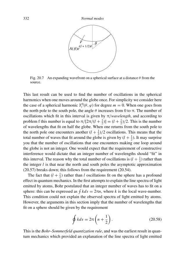
332 Normal modes
A( )ei(l + 1/2)
Fig. 20.7 An expanding wavefront on a spherical surface at a distance θ from thesource.
This last result can be used to find the number of oscillations in the sphericalharmonics when one moves around the globe once. For simplicity we consider herethe case of a spherical harmonic Y 0
l (θ, ϕ) for degree m = 0. When one goes fromthe north pole to the south pole, the angle θ increases from 0 to π. The number ofoscillations which fit in this interval is given by π/wavelength, and according toproblem f this number is equal to π/[2π/(l + 1
2 )] = (l + 12 )/2. This is the number
of wavelengths that fit on half the globe. When one returns from the south pole tothe north pole one encounters another (l + 1
2 )/2 oscillations. This means that thetotal number of waves that fit around the globe is given by (l + 1
2 ). It may surpriseyou that the number of oscillations that one encounters making one loop aroundthe globe is not an integer. One would expect that the requirement of constructiveinterference would dictate that an integer number of wavelengths should “fit” inthis interval. The reason why the total number of oscillations is (l + 1
2 ) rather thanthe integer l is that near the north and south poles the asymptotic approximation(20.57) breaks down; this follows from the requirement (20.54).
The fact that (l + 12 ) rather than l oscillations fit on the sphere has a profound
effect in quantum mechanics. In the first attempts to explain the line spectra of lightemitted by atoms, Bohr postulated that an integer number of waves has to fit on asphere: this can be expressed as
∮
kds = 2πn, where k is the local wave-number.This condition could not explain the observed spectra of light emitted by atoms.However, the arguments in this section imply that the number of wavelengths thatfit on a sphere should be given by the requirement
∮
kds = 2π
(
n + 1
2
)
. (20.58)
This is the Bohr–Sommerfeld quantization rule, and was the earliest result in quan-tum mechanics which provided an explanation of the line spectra of light emitted
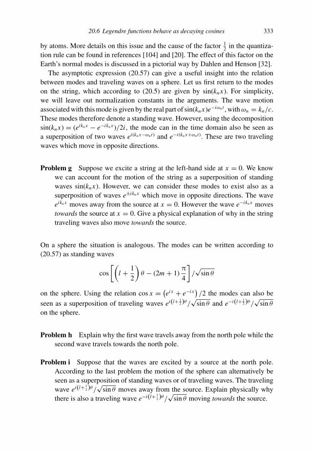
20.6 Legendre functions behave as decaying cosines 333
by atoms. More details on this issue and the cause of the factor 12 in the quantiza-
tion rule can be found in references [104] and [20]. The effect of this factor on theEarth’s normal modes is discussed in a pictorial way by Dahlen and Henson [32].
The asymptotic expression (20.57) can give a useful insight into the relationbetween modes and traveling waves on a sphere. Let us first return to the modeson the string, which according to (20.5) are given by sin(knx). For simplicity,we will leave out normalization constants in the arguments. The wave motionassociated with this mode is given by the real part of sin(knx)e−iωn t , with ωn = kn/c.These modes therefore denote a standing wave. However, using the decompositionsin(knx) = (eikn x − e−ikn x )/2i , the mode can in the time domain also be seen asa superposition of two waves ei(kn x−ωn t) and e−i(kn x+ωn t). These are two travelingwaves which move in opposite directions.
Problem g Suppose we excite a string at the left-hand side at x = 0. We knowwe can account for the motion of the string as a superposition of standingwaves sin(knx). However, we can consider these modes to exist also as asuperposition of waves e±ikn x which move in opposite directions. The waveeikn x moves away from the source at x = 0. However the wave e−ikn x movestowards the source at x = 0. Give a physical explanation of why in the stringtraveling waves also move towards the source.
On a sphere the situation is analogous. The modes can be written according to(20.57) as standing waves
cos
[(
l + 1
2
)
θ − (2m + 1)π
4
]
/√
sin θ
on the sphere. Using the relation cos x = (eix + e−i x)
/2 the modes can also be
seen as a superposition of traveling waves ei(l+ 12 )θ/
√sin θ and e−i(l+ 1
2 )θ/√
sin θ
on the sphere.
Problem h Explain why the first wave travels away from the north pole while thesecond wave travels towards the north pole.
Problem i Suppose that the waves are excited by a source at the north pole.According to the last problem the motion of the sphere can alternatively beseen as a superposition of standing waves or of traveling waves. The travelingwave ei(l+ 1
2 )θ/√
sin θ moves away from the source. Explain physically whythere is also a traveling wave e−i(l+ 1
2 )θ/√
sin θ moving towards the source.

334 Normal modes
These results imply that the oscillations of the Earth can be seen as either a super-position of normal modes, or a superposition of waves that travel along the Earth’ssurface in opposite directions. The waves that travel along the Earth’s surface arecalled surface waves. The relation between normal modes and surface waves istreated in more detail by Dahlen [31] and by Snieder and Nolet [101].
20.7 Normal modes and the Green’s function
In Section 13.6 we analyzed the normal modes of a system of three coupled masses.This system had three normal modes, and each mode could be characterized by avector v(n) with the displacement of the three masses and by an eigenfrequencyωn . The response of the system to a force F acting on the three masses with timedependence e−iωt was derived to be:
x = 1
m
3∑
n=1
v(n)(v(n) · F)(
ω2n − ω2
) . (13.67)
This means that the Green’s function of this system is given by the following dyad:
G = 1
2πm
3∑
n=1
v(n)v(n)T
(
ω2n − ω2
) . (20.59)
The factor 1/2π is due to the fact that a delta-function force f (t) = δ(t) in thetime domain corresponds with the Fourier transform (15.43) to F(ω) = 1/2π inthe frequency domain. In this section we derive the Green’s function for a generaloscillating system that can be continuous. An important example is the Earth,which is a body that has well-defined normal modes and where the displacement isa continuous function of the space coordinates.
We consider a system that satisfies the following equation of motion:
ρu + Hu = F. (20.60)
The field u can be either a scalar field or a vector field. The operator H at this pointis general, the only requirement that we impose is that this operator is Hermitian,which means that we require that
( f · Hg) = (H f · g) , (20.61)
where the inner product is defined as ( f · h) ≡ ∫ f ∗g dV . In the frequency domain,the equation of motion is given by
−ρω2u + Hu = F(ω). (20.62)

20.7 Normal modes and the Green’s function 335
Let the normal modes of the system be denoted by u(n); the normal modesdescribe the oscillations of the system in the absence of any external force. Thenormal modes therefore satisfy the following expression
Hu(n) = ρω2nu(n), (20.63)
where ωn is the eigenfrequency of this mode.
Problem a Take the inner product of this expression with a mode u(m), and usethe fact that H is Hermitian to derive that
(
ω2n − ω∗2
m
) (
u(m) · ρu(n)) = 0. (20.64)
Note the resemblance of this expression to (20.40) for the modes of a system thatobeys the Helmholtz equation.
Problem b Just like in Section 20.4 one can show that the eigenfrequencies arereal by setting m = n, and one can derive that different modes are orthogonalwith respect to the following inner product:
(
u(m) · ρu(n)) = δnm for ωm = ωn. (20.65)
Use (20.64) to give a proof of this orthogonality relation.
Note the presence of the density term ρ in this inner product.In the analysis of this section it was crucial for the operator H to be Hermitian.
This property of H has two important implications: (1) the eigenvalues of H arereal and (2) the eigenfunctions are orthogonal. It is for this reason that it is crucialto establish whether the operator H is Hermitian or not. In general, the operator of adynamical system is Hermitian when the system is invariant for time-reversal. Thismeans that the equations are invariant when one lets the clock run backward, ormathematically when one replaces t by −t . Dissipation in general breaks the sym-metry for time-reversal. It is shown in detail by Dahlen and Tromp [33] that attenu-ation in the Earth makes the eigenfrequencies of the Earth complex and that the nor-mal modes of an attenuating Earth do not satisfy the orthogonality relation (20.65).
Let us now return to the inhomogeneous problem (20.62) where an external forceF(ω) is present. Assuming that the normal modes form a complete set, the responseto this force can be written as a sum of normal modes:
u =∑
n
cnu(n), (20.66)
where the cn are unknown coefficients.

336 Normal modes
Problem c Find these coefficients by inserting (20.66) into the equation of motion(20.62) and by taking the inner product of the result with a mode u(m) to derivethat
cm =(
u(m) · F)
ω2m − ω2
. (20.67)
This means that the response of the system can be written as:
u =∑
n
u(n)(
u(n) · F)
ω2n − ω2
. (20.68)
Note the resemblance of this expression to (13.67) for a system of three masses.The main difference is that the derivation in this section is also valid for continuousvibrating systems such as the Earth.
It is instructive to rewrite this expression taking the dependence of the spacecoordinates explicitly into account:
u(r) =∑
n
u(n)(r)∫
u∗(n)(r′)F(r′) dV ′
ω2n − ω2
. (20.69)
It follows from this expression that the Green’s function is given by
G(r, r′, ω) = 1
2π
∑
n
u(n)(r)u∗(n)(r′)ω2
n − ω2. (20.70)
When the mode is a vector, one should take the transpose of the mode u∗(n)(r′).Note the similarity between this expression for the Green’s function of a continuousmedium and the Green’s function (20.59) for a discrete system. In this sense, theEarth behaves in the same way as a tri-atomic molecule. For both systems, thedyadic representation of the Green’s function provides a compact way to accountfor the response of the system to external forces.
Note that the response is strongest when the frequency ω of the external forceis close to one of the eigenfrequencies ωn of the system. This implies for examplefor the Earth that modes with a frequency close to the frequency of the externalforcing are most strongly excited. If we jump up and down with a frequency of1 Hz, we excite the Earth’s fundamental mode with a period of about 1 hour onlyvery weakly. In addition, a mode is most effectively excited when the inner productof the forcing F(r′) in (20.69) is maximal. This means that a mode is most stronglyexcited when the spatial distribution of the force equals the displacement u(n)(r′)of the mode.
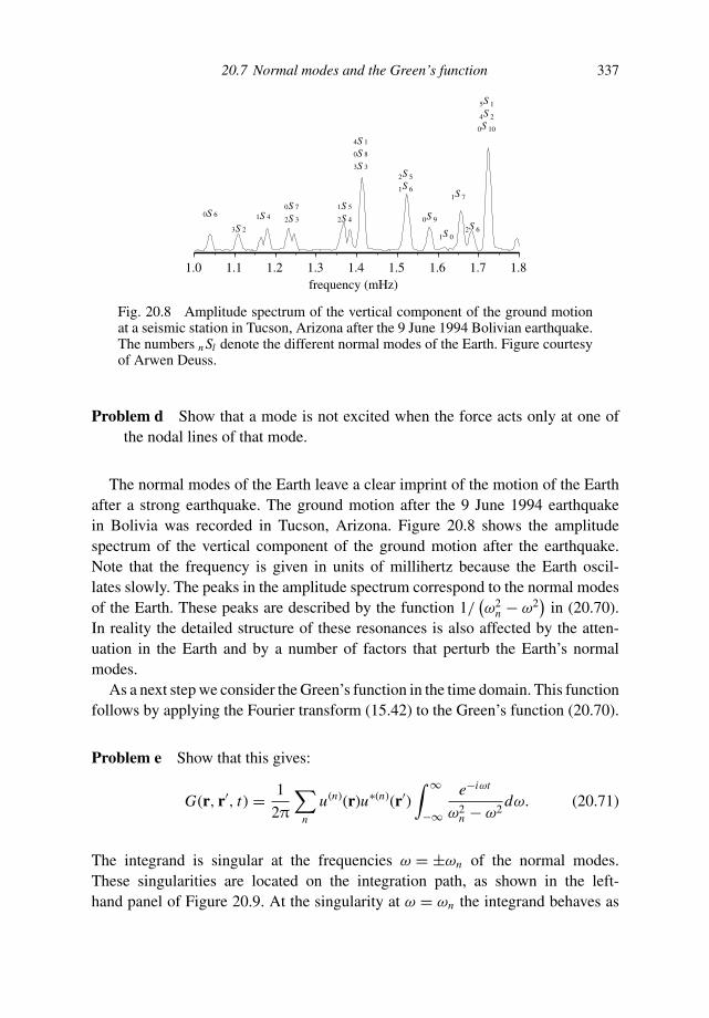
20.7 Normal modes and the Green’s function 337
1.0 1.1 1.2 1.3 1.4 1.5 1.6 1.7 1.8frequency (mHz)
0S 6
3S 2
1S 40S 7
2S 3
1S 5
2S 4
4S 1
0S 8
3S 32S 5
1S 6
0S 9
1S 0
1S 7
2S 6
5S 1
4S 2
0S 10
Fig. 20.8 Amplitude spectrum of the vertical component of the ground motionat a seismic station in Tucson, Arizona after the 9 June 1994 Bolivian earthquake.The numbers n Sl denote the different normal modes of the Earth. Figure courtesyof Arwen Deuss.
Problem d Show that a mode is not excited when the force acts only at one ofthe nodal lines of that mode.
The normal modes of the Earth leave a clear imprint of the motion of the Earthafter a strong earthquake. The ground motion after the 9 June 1994 earthquakein Bolivia was recorded in Tucson, Arizona. Figure 20.8 shows the amplitudespectrum of the vertical component of the ground motion after the earthquake.Note that the frequency is given in units of millihertz because the Earth oscil-lates slowly. The peaks in the amplitude spectrum correspond to the normal modesof the Earth. These peaks are described by the function 1/
(
ω2n − ω2
)
in (20.70).In reality the detailed structure of these resonances is also affected by the atten-uation in the Earth and by a number of factors that perturb the Earth’s normalmodes.
As a next step we consider the Green’s function in the time domain. This functionfollows by applying the Fourier transform (15.42) to the Green’s function (20.70).
Problem e Show that this gives:
G(r, r′, t) = 1
2π
∑
n
u(n)(r)u∗(n)(r′)∫ ∞
−∞
e−iωt
ω2n − ω2
dω. (20.71)
The integrand is singular at the frequencies ω = ±ωn of the normal modes.These singularities are located on the integration path, as shown in the left-hand panel of Figure 20.9. At the singularity at ω = ωn the integrand behaves as

338 Normal modes
x xx x
? ?
Fig. 20.9 The location of the poles and the integration path in the complex ω-plane. The poles are indicated with a cross. The left-hand panel shows the originalsituation where the poles are located on the integration path at location ±ωn . Theright-hand panel shows the location of the poles when a slight anelastic dampingis present.
1/[2ωn(ω − ωn)]. The contribution of these singularities is poorly defined becausethe integral
∫
1/ (ω − ωn) dω is not defined.This situation is comparable to the treatment in Section 17.4 of the response
of a particle in syrup to an external forcing. When this particle was subjectedto a damping β, the integrand in the Fourier transform to the time domain had asingularity in the lower half-plane. This gave a causal response; as shown in (17.35)the response was different from zero only at times later than the time at which theforcing was applied. This suggests that we can obtain a well-defined causal responseof the Green’s function (20.71) when we introduce a slight damping. This dampingbreaks the invariance of the problem for time-reversal, and is responsible for acausal response. At the end of the calculation we can let the damping parameter goto zero. Damping can be introduced by giving the eigenfrequencies of the normalmodes a small negative imaginary component: ±ωn → ±ωn − iη, where η is asmall positive number.
Problem f The time dependence of the oscillation of a normal mode is given bye−iωn t . Show that with this replacement the modes decay with a decay timethat is given by
τ = 1/η. (20.72)
This last property means that when we ultimately set η = 0 the decay time becomesinfinite: in other words, the modes are not attenuated in that limit.
With the replacement ±ωn → ±ωn − iη the poles that are associated withthe normal modes are located in the lower ω-plane: this situation is shown in
20.7 Normal modes and the Green’s function 339
Figure 20.9. Now that the singularities are moved from the integration path, thetheory of complex integration can be used to evaluate the resulting integral.
Problem g Use the theory of contour integration as treated in Chapter 17 to derivethat the Green’s function is given in the time domain by:
G(r, r′, t) =
⎧
⎪
⎪
⎨
⎪
⎪
⎩
0 for t < 0
∑
n
u(n)(r)u∗(n)(r′)ωn
sin ωnt for t > 0. (20.73)
Hint: use the same steps as in the derivation of the function (17.35) and let thedamping parameter η go to zero at the end of the integration.
This result gives a causal response because the Green’s function is only nonzeroat times t > 0, which is later than the time t = 0 when the delta-function forcing isnonzero. The total response is given as a sum over all the modes. Each mode leadsto a time signal sin(ωnt) in the modal sum: this is a periodic oscillation with thefrequency ωn of the mode. The singularities in the integrand of the Green’s function(20.71) at the pole positions ω = ±ωn are thus associated in the time domain witha harmonic oscillation with angular frequency ωn . Note that the Green’s function iscontinuous at the time t = 0 of excitation. It is interesting to compare this Green’sfunction with the Green’s function (18.21) for the girl on the swing. The onlydifferences are that in (20.73) modes are present in the Green’s function and that asummation over the modes is carried out. This difference is due to the fact that theharmonic oscillator has only one mode and that this mode of oscillation does nothave a spatial extent.
Problem h Use the Green’s function (20.73) to derive that the response of thesystem to a force F(r, t) is given by:
u(r, t) =∑
n
1
ωnu(n)(r)
∫ ∫ t
−∞u∗(n)(r′) sin ωn
(
t − t ′) F(r′, t ′) dt ′dV ′.
(20.74)
Justify the integration limit in the t ′-integration.
The results in this section imply that the total Green’s function of a system is knownonce the normal modes are known. The total response can then be obtained bysumming the contribution of each normal mode to the total response. This techniqueis called normal-mode summation, and is often used to obtain the low-frequencyresponse of the Earth to an excitation [33, 35]. However, in the seismological

340 Normal modes
literature one usually treats a source signal that is given by a step function at t = 0rather than a delta function because this is a more accurate description of the slipon a fault during an earthquake [3]. This leads to a time dependence (1 − cos(ωnt))rather than the time dependence sin(ωnt) in the response (20.73) to a delta-functionexcitation.
20.8 Guided waves in a low-velocity channel
In this section we consider a system that strictly speaking does not have normalmodes, but that can support solutions that behave like traveling waves in one di-rection and as modes in another direction. The waves in such a system propagateas guided waves. Consider a system in two dimensions (x and z), where the veloc-ity depends only on the z-coordinate. We assume that the wave-field satisfies theHelmholtz equation (20.1) in the frequency domain:
∇2u + ω2
c2(z)u = 0. (20.75)
In this section we consider a simple model of a layer of thickness H that extendsfrom z = 0 to z = H in which the velocity is given by c1. This layer is embeddedin a medium with a constant velocity c0. The geometry of the problem is shown inFigure 20.10. Since the system is invariant in the x-direction, the problem can besimplified by a Fourier transform over the x-coordinate:
u(x, z) =∫ ∞
−∞U (k, z)eikx dk. (20.76)
Problem a Show that U (k, z) satisfies the following ordinary differential equa-tion:
d2U
dz2+[
ω2
c(z)2− k2
]
U = 0. (20.77)
z = H
z = 0
c
c
c0
1
0
Fig. 20.10 Geometry of the model of a single layer sandwiched between twohomogeneous half-spaces.
20.8 Guided waves in a low-velocity channel 341
It is important to note at this point that the frequency ω is a fixed constant, andthat according to (20.76) the variable k is an integration variable that assumes allvalues in the integration (20.76). For this reason one should not at this point use therelation k = ω/c(z).
Now consider the special case of the model shown in Figure 20.10. We requirethat the waves outside the layer move away from the layer.
Problem b Show that this implies that the solution for z < 0 is given by Ae−ik0z
and the solution for z > H is given by Be+ik0z where A and B are unknownintegration constants and where k0 is given by
k0 =√
ω2
c20
− k2. (20.78)
Problem c Show that within the layer the wave field is given by C cos(k1z) +D sin(k1z) with C and D integration constants and k1 given by
k1 =√
ω2
c21
− k2. (20.79)
The solution in the three regions of space therefore takes the following form:
U (k, z) =⎧
⎨
⎩
Ae−ik0z for z < 0C cos(k1z) + D sin(k1z) for 0 < z < H.
Be+ik0z for z > H(20.80)
We now have the general form of the solution within the layer and the twohalf-spaces on either side of the layer. Boundary conditions are needed to findthe integration constants A, B, C , and D. For this system both U and dU/dz arecontinuous at z = 0 and z = H .
Problem d Use the results of problem b and problem c to show that these require-ments impose the following constraints on the integration constants:
A − C = 0,
ik0 A + k1 D = 0,
−Beik0 H + C cos k1 H + D sin k1 H = 0,
ik0 Beik0 H + k1C cos k1 H − k1 D sin k1 H = 0.
⎫
⎪
⎪
⎬
⎪
⎪
⎭
(20.81)
This is a linear system of four equations for the four unknowns A, B, C , and D.Note that this is a homogeneous system of equations, because the right-hand sides

342 Normal modes
vanish. Such a homogeneous system of equations only has nonzero solutions whenthe determinant of the system of equations vanishes.
Problem e Show that this requirement leads to the following condition:
tan(k1 H ) = −2ik0k1
k21 + k2
0
. (20.82)
This equation is implicitly an equation for the wave-number k, because accordingto (20.78) and (20.79) both k0 and k1 are functions of the wave-number k. Equa-tion (20.82) implies that the system can only support waves when the wavenum-ber k is such that expression (20.82) is satisfied. The system, strictly speaking,does not have normal modes, because the waves propagate in the x-direction.However, in the z-direction the waves only “fit” in the layer for very specificvalues of the wavenumber k. These waves are called “guided waves” becausethey propagate along the layer with a well-defined phase velocity that followsfrom the relation c(ω) = ω/k. Be careful not to confuse this phase velocity c(ω)with the velocities c1 and c0 in the layer and the half-spaces outside the layer.At this point we do not know yet what the phase velocities of the guided wavesare.
The phase velocity follows from expression (20.82) because this expressionis implicitly an equation for the wavenumber k. At this point we consider thecase of a low-velocity layer, that is we assume that c1 < c0. In this case 1/c0 <
1/c1. We look for guided waves with a wavenumber in the following interval:ω/c0 < k < ω/c1.
Problem f Show that in that case k1 is real and k0 is purely imaginary. Writek0 = iκ0 and show that
κ0 =√
k2 − ω2
c20
. (20.83)
Problem g Show that the solution decays exponentially away from thelow-velocity channel both in the half-space z < 0 and the half-spacez > H .
The fact that the waves decay exponentially with the distance to the low-velocitylayer means that the guided waves are trapped near the low-velocity layer. Wavesthat decay exponentially are called evanescent waves.
20.8 Guided waves in a low-velocity channel 343
Problem h Use (20.82) to show that the wavenumber of the guided waves satisfiesthe following relation:
tan
√
ω2
c21
− k2 H =2
√
k2 − ω2
c20
√
ω2
c21
− k2
ω2
(
1
c21
− 1
c20
) . (20.84)
For a fixed value of ω this expression constitutes a constraint on the wavenumberk of the guided waves. Unfortunately, it is not possible to solve this equation for kin closed form. Such an equation is called a transcendental equation.
Problem j Make a sketch of both the left-hand side and the right-hand side of(20.84) as a function of k. Show that the two curves have a finite number ofintersection points.
These intersection points correspond to the k-values of the guided waves. Thecorresponding phase velocity c = ω/k in general depends on the frequency ω.This means that these guided waves are dispersive, which means that the differentfrequency components travel with a different phase velocity. It is for this reasonthat (20.84) is called the dispersion relation.
Dispersive waves occur in many different situations. When electromagneticwaves propagate between plates or in a layered structure, guided waves result [53].The atmosphere, and most importantly the ionosphere, is an excellent waveguide forelectromagnetic waves [47]. This leads to a large variety of electromagnetic guidedwaves in the upper atmosphere with exotic names such as “pearls”, “whistlers”,“tweaks”, “hydromagnetic howling”, and “serpentine emissions”; colorful namesassociated with the sounds these phenomena would make if they were audible, orwith the patterns they generate in frequency–time diagrams. These perturbations areexcited for example by the electromagnetic fields generated by lightning. Guidedwaves play a crucial role in telecommunication, because light propagates throughoptical fibers as guided waves [61]. The fact that these waves are guided prohibitsthe light from propagating out of the fiber, and this allows for the transmission oflight signals over extremely large distances.
In the Earth the wave velocity increases rapidly with depth. Elastic waves canbe guided near the Earth’s surface and the different modes are called “Rayleighwaves” and “Love waves” [3]. These surface waves in the Earth are a prime toolfor mapping the shear velocity within the Earth [98].
Since the surface waves in the Earth are trapped near the Earth’s surface, theyeffectively propagate in two dimensions rather than in three dimensions. The surface
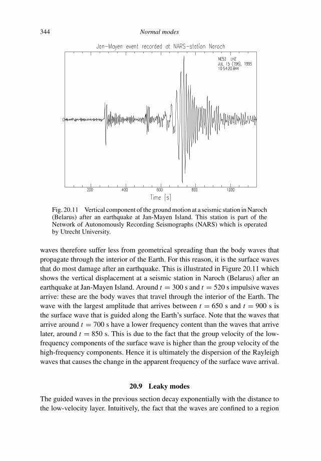
344 Normal modes
Fig. 20.11 Vertical component of the ground motion at a seismic station in Naroch(Belarus) after an earthquake at Jan-Mayen Island. This station is part of theNetwork of Autonomously Recording Seismographs (NARS) which is operatedby Utrecht University.
waves therefore suffer less from geometrical spreading than the body waves thatpropagate through the interior of the Earth. For this reason, it is the surface wavesthat do most damage after an earthquake. This is illustrated in Figure 20.11 whichshows the vertical displacement at a seismic station in Naroch (Belarus) after anearthquake at Jan-Mayen Island. Around t = 300 s and t = 520 s impulsive wavesarrive: these are the body waves that travel through the interior of the Earth. Thewave with the largest amplitude that arrives between t = 650 s and t = 900 s isthe surface wave that is guided along the Earth’s surface. Note that the waves thatarrive around t = 700 s have a lower frequency content than the waves that arrivelater, around t = 850 s. This is due to the fact that the group velocity of the low-frequency components of the surface wave is higher than the group velocity of thehigh-frequency components. Hence it is ultimately the dispersion of the Rayleighwaves that causes the change in the apparent frequency of the surface wave arrival.
20.9 Leaky modes
The guided waves in the previous section decay exponentially with the distance tothe low-velocity layer. Intuitively, the fact that the waves are confined to a region

20.9 Leaky modes 345
near a low-velocity layer can be understood as follows. Waves are refracted fromregions of high velocity to a region of low velocity. This means that the waves thatstray out of the low-velocity channel are refracted back into the channel. Effectivelythis traps the waves in the vicinity of the channel. This explanation suggests thatfor a high-velocity channel the waves are refracted away from the channel. Theresulting wave pattern then corresponds to waves that preferentially move awayfrom the high-velocity layer. For this reason we consider in this section the wavesthat propagate through the system shown in Figure 20.10 but now we consider thecase of a high-velocity layer where c1 > c0.
In this case, 1/c1 < 1/c0, and we consider waves with a wavenumber that isconfined to the following interval: ω/c1 < k < ω/c0.
Problem a Show that in this case the wavenumber k1 is imaginary and that it canbe written as k1 = iκ1, with
κ1 =√
k2 − ω2
c21
, (20.85)
and show that the dispersion relation (20.82) is given by:
tan(iκ1 H ) = −2k0κ1
κ21 − k2
0
. (20.86)
Problem b Use the relation cos x = (eix + e−i x)
/2 and the related expressionfor sin x to rewrite the dispersion relation (20.86) in the following form:
i tanh(κ1 H ) = −2k0κ1
κ21 − k2
0
. (20.87)
In this expression all quantities are real when k is real. The factor i on the left-handside implies that this equation cannot be satisfied for real values of k. The onlyway in which the dispersion relation (20.87) can be satisfied is if k is complex.What does it mean if the wavenumber is complex? Suppose that the dispersionrelation is satisfied for a complex wavenumber k = kr + iki , with kr and ki the realand imaginary parts. In the time domain a solution behaves for a fixed frequency asU (k, z)ei(kx−ωt). This means that for complex values of the wavenumber the solutionbehaves as U (k, z)e−ki x ei(kr x−ωt). This is a wave that propagates in the x-directionwith phase velocity c = ω/kr and that decays exponentially with the propagationdistance x .
The exponential decay of the wave with the propagation distance x is due to thefact that the wave energy refracts out of the high-velocity layer. A different way of
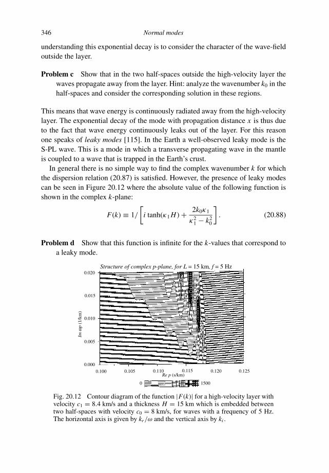
346 Normal modes
understanding this exponential decay is to consider the character of the wave-fieldoutside the layer.
Problem c Show that in the two half-spaces outside the high-velocity layer thewaves propagate away from the layer. Hint: analyze the wavenumber k0 in thehalf-spaces and consider the corresponding solution in these regions.
This means that wave energy is continuously radiated away from the high-velocitylayer. The exponential decay of the mode with propagation distance x is thus dueto the fact that wave energy continuously leaks out of the layer. For this reasonone speaks of leaky modes [115]. In the Earth a well-observed leaky mode is theS-PL wave. This is a mode in which a transverse propagating wave in the mantleis coupled to a wave that is trapped in the Earth’s crust.
In general there is no simple way to find the complex wavenumber k for whichthe dispersion relation (20.87) is satisfied. However, the presence of leaky modescan be seen in Figure 20.12 where the absolute value of the following function isshown in the complex k-plane:
F(k) ≡ 1/
[
i tanh(κ1 H ) + 2k0κ1
κ21 − k2
0
]
. (20.88)
Problem d Show that this function is infinite for the k-values that correspond toa leaky mode.
0. 15000
0.100 0.105 0.115 0.120 0.125
0.020
0.015
0.010
0.005
0.000
Imwp
(1/
km)
Re p (s/km)0.110
Structure of complex p-plane, for L = 15 km, f = 5 Hz
Fig. 20.12 Contour diagram of the function |F(k)| for a high-velocity layer withvelocity c1 = 8.4 km/s and a thickness H = 15 km which is embedded betweentwo half-spaces with velocity c0 = 8 km/s, for waves with a frequency of 5 Hz.The horizontal axis is given by kr/ω and the vertical axis by ki .
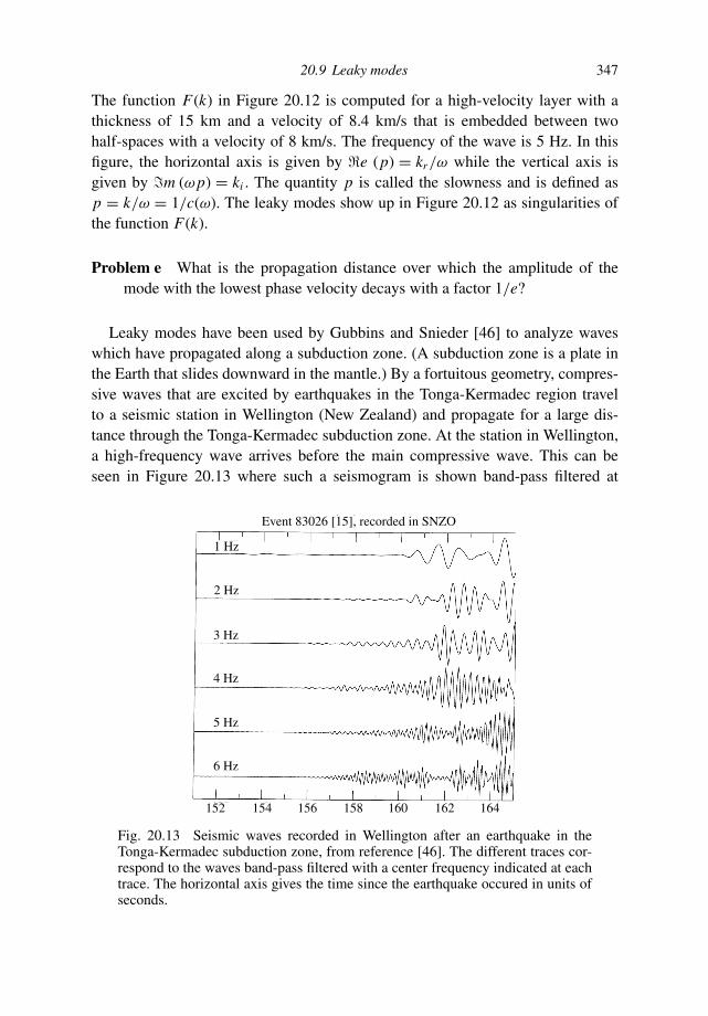
20.9 Leaky modes 347
The function F(k) in Figure 20.12 is computed for a high-velocity layer with athickness of 15 km and a velocity of 8.4 km/s that is embedded between twohalf-spaces with a velocity of 8 km/s. The frequency of the wave is 5 Hz. In thisfigure, the horizontal axis is given by e (p) = kr/ω while the vertical axis isgiven by m (ωp) = ki . The quantity p is called the slowness and is defined asp = k/ω = 1/c(ω). The leaky modes show up in Figure 20.12 as singularities ofthe function F(k).
Problem e What is the propagation distance over which the amplitude of themode with the lowest phase velocity decays with a factor 1/e?
Leaky modes have been used by Gubbins and Snieder [46] to analyze waveswhich have propagated along a subduction zone. (A subduction zone is a plate inthe Earth that slides downward in the mantle.) By a fortuitous geometry, compres-sive waves that are excited by earthquakes in the Tonga-Kermadec region travelto a seismic station in Wellington (New Zealand) and propagate for a large dis-tance through the Tonga-Kermadec subduction zone. At the station in Wellington,a high-frequency wave arrives before the main compressive wave. This can beseen in Figure 20.13 where such a seismogram is shown band-pass filtered at
152 154 156 158 160 162 164
6 Hz
5 Hz
4 Hz
3 Hz
2 Hz
1 Hz
Event 83026 [15], recorded in SNZO
Fig. 20.13 Seismic waves recorded in Wellington after an earthquake in theTonga-Kermadec subduction zone, from reference [46]. The different traces cor-respond to the waves band-pass filtered with a center frequency indicated at eachtrace. The horizontal axis gives the time since the earthquake occured in units ofseconds.

348 Normal modes
different frequencies. It can clearly be seen that waves with a frequency around6 Hz arrive before waves with a frequency around 1 Hz. This observation canbe explained by the propagation of a leaky mode through the subduction zone.The physical reason why the high-frequency components arrive before the lower-frequency components is that the high-frequency waves “fit” in the high-velocitylayer in the subducting plate, whereas the lower-frequency components do not fitin the high-velocity layer and are more influenced by the slower material outsidethe high-velocity layer. Of course, the energy leaks out of the high-velocity layerso that this arrival is very weak. From the data it could be inferred that in thesubduction zone a high-velocity layer with a thickness between 6 and 10 km ispresent [46].
20.10 Radiation damping
Up to this point we have considered systems that are freely oscillating. When suchsystems are of finite extent, such a system displays undamped free oscillations.In the previous section leaky modes were introduced. In such a system, energy isradiated away, which leads to an exponential decay of waves that propagate throughthe system. In a similar way, a system that has normal modes when it is isolatedfrom its surroundings can display damped oscillations when it is coupled to theexternal world.
As a simple prototype of such a system, consider a mass m that can move inthe z-direction which is coupled to a spring with spring constant κ . The mass isattached to a string which is under a tension T and which has a mass ρ per unitlength. The system is shown in Figure 20.14. The total force acting on the mass isthe sum of the force −κz exerted by the spring and the force Fs that is generatedby the string:
mz + κz = Fs, (20.89)
x
z
Fig. 20.14 Geometry of an oscillating mass that is coupled to a spring.

20.10 Radiation damping 349
where z denotes the vertical displacement of the mass. The motion of the wavesthat propagate in the string is given by the wave equation:
uxx − 1
c2utt = 0, (20.90)
where u is the displacement of the string in the vertical direction and c is given by
c =√
T
ρ. (20.91)
Let us first consider the case in which no external force is present and the massis not coupled to the spring.
Problem a Show that in that case the equation of motion is given by
z + ω20z = 0, (20.92)
with ω0 given by
ω0 =√
κ
m. (20.93)
One can say that the mass that is not coupled to the string has one free oscillationwith angular frequency ω0. The fact that the system has one free oscillation is aconsequence of the fact that this mass can move in the vertical direction only, henceit has only one degree of freedom.
Before we couple the mass to the string let us first analyze the wave motion inthe string in the absence of the mass.
Problem b Show that any function f (t − x/c) satisfies the wave equation (20.90).Show that this function describes a wave that moves in the positive x-directionwith velocity c.
Problem c Show that any function g(t + x/c) satisfies the wave equation (20.90)as well. Show that this function describes a wave that moves in the negativex-direction with velocity c.
The general solution is a superposition of the rightward and leftward moving waves:
u(x, t) = f(
t − x
c
)
+ g(
t + x
c
)
. (20.94)
This general solution is called the d’Alembert solution.
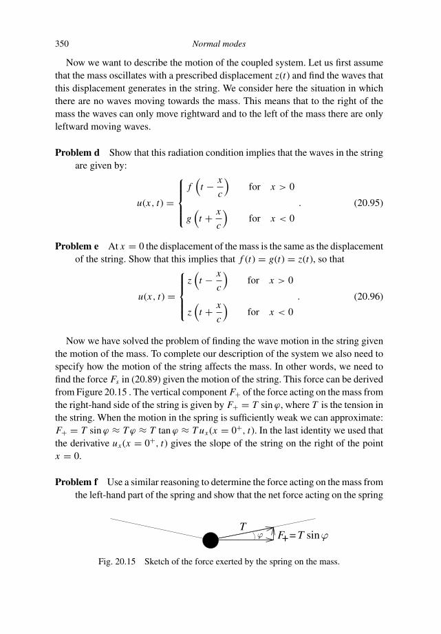
350 Normal modes
Now we want to describe the motion of the coupled system. Let us first assumethat the mass oscillates with a prescribed displacement z(t) and find the waves thatthis displacement generates in the string. We consider here the situation in whichthere are no waves moving towards the mass. This means that to the right of themass the waves can only move rightward and to the left of the mass there are onlyleftward moving waves.
Problem d Show that this radiation condition implies that the waves in the stringare given by:
u(x, t) =
⎧
⎪
⎪
⎨
⎪
⎪
⎩
f(
t − x
c
)
for x > 0
g(
t + x
c
)
for x < 0
. (20.95)
Problem e At x = 0 the displacement of the mass is the same as the displacementof the string. Show that this implies that f (t) = g(t) = z(t), so that
u(x, t) =
⎧
⎪
⎪
⎨
⎪
⎪
⎩
z(
t − x
c
)
for x > 0
z(
t + x
c
)
for x < 0
. (20.96)
Now we have solved the problem of finding the wave motion in the string giventhe motion of the mass. To complete our description of the system we also need tospecify how the motion of the string affects the mass. In other words, we need tofind the force Fs in (20.89) given the motion of the string. This force can be derivedfrom Figure 20.15 . The vertical component F+ of the force acting on the mass fromthe right-hand side of the string is given by F+ = T sin ϕ, where T is the tension inthe string. When the motion in the spring is sufficiently weak we can approximate:F+ = T sin ϕ ≈ T ϕ ≈ T tan ϕ ≈ T ux (x = 0+, t). In the last identity we used thatthe derivative ux (x = 0+, t) gives the slope of the string on the right of the pointx = 0.
Problem f Use a similar reasoning to determine the force acting on the mass fromthe left-hand part of the spring and show that the net force acting on the spring
TF+= T sin
Fig. 20.15 Sketch of the force exerted by the spring on the mass.

20.10 Radiation damping 351
is given by
Fs(t) = T(
ux (x = 0+, t) − ux (x = 0−, t))
, (20.97)
where ux (x = 0−, t) is the x-derivative of the displacement in the string justto the left of the mass.
Problem g Show that this expression implies that the net force that acts on themass is equal to the kink in the spring at the location of the mass.
You may not feel comfortable with the fact the we used the approximation of a smallangle ϕ in the derivation of (20.97). However, keep in mind that the wave equa-tion (20.90) is derived using the same approximation and that this wave equationtherefore is only valid for small displacements of the string.
At this point we have assembled all the ingredients for solving the coupledproblem.
Problem h Use (20.96) and (20.97) to derive that the force exerted by the springon the mass is given by
Fs(t) = −2T
cz, (20.98)
and that the motion of the mass is therefore given by:
z + 2T
mcz + ω2
0z = 0. (20.99)
It is interesting to compare this expression for the motion of the mass that iscoupled to the string with the equation of motion (20.92) for the mass that is notcoupled to the string. The string leads to a term (2T/mc) z in the equation of motionthat damps the motion of the mass. How can we explain this damping physically?When the mass moves, the string moves with it at location x = 0. Any motion inthe string at that point excites waves propagating in the string. This means that thestring radiates wave energy away from the mass whenever the mass moves. Sinceenergy is conserved, the energy that is radiated in the string must be withdrawn fromthe energy of the moving mass. This means that the mass loses energy wheneverit moves; this effect is described by the damping term in equation (20.99). Thisdamping process is called radiation damping, because it is the radiation of wavesthat damps the motion of the mass.
The system described in this section is extremely simple. However, it does containthe essential physics of radiation damping. Many systems in physics that displaynormal modes are not quite isolated from their surroundings. Interactions of the

352 Normal modes
systems with their surroundings often lead to the radiation of energy, and hence toa damping of the oscillation of the system.
One example of such a system is an atom in an excited state. In the absenceof external influences such an atom will not emit any light and will not decay.However, when such an atom can interact with electromagnetic fields, it can emita photon and subsequently decay.
A second example is a charged particle that moves in a synchrotron. In the absenceof external fields, such a particle will continue forever in a circular orbit without anychange in its speed. In reality, a charged particle is coupled to electromagnetic fields.This has the effect that a charged particle that is accelerated emits electromagneticradiation, called synchrotron radiation [53]. The radiated energy corresponds toan energy loss of the particle, so that the particle slows down. This is actually thereason why accelerators such as those used at CERN and Fermilab are so large.The acceleration of a particle in a circular orbit with radius r at the given velocityv is given by v2/r . This means that for a fixed velocity v the larger is the radiusof the orbit, the smaller is the acceleration, and the weaker is the energy loss dueto the emission of synchrotron radiation. This is why one needs huge machines toaccelerate tiny particles to an extreme energy.
Problem i The modes in the plate in Figure 20.1 are also damped because ofradiation damping. What form of radiation is emitted by this oscillating plate?

21
Potential theory
Potential fields play an important role in physics and geophysics because theydescribe the behavior of gravitational and electric fields as well as a number of otherfields. Conversely, measurements of potential fields provide important informationabout the internal structure of bodies. For example, measurements of the electricpotential at the Earth’s surface when a current is sent into the Earth give informationabout the electrical conductivity while measurements of the Earth’s gravity field orgeoid provide information about the mass distribution within the Earth.
An example of this can be seen in Figure 21.1 in which the gravity anomalyover the northern part of the Yucatan peninsula in Mexico is shown [49]. Thecoast is visible as a thin white line. Note the ring structure that is visible in thegravity signal. These rings have led to the discovery of the Chicxulub crater whichwas caused by the massive impact of a meteorite. Note that the diameter of theimpact crater is about 150 km! This crater is presently hidden by thick layers ofsediments: at the surface the only apparent imprint of this crater is the presence ofunderground water-filled caves called “cenotes” at the outer edge of the crater. Itwas the measurement of the gravity field that made it possible to find this massiveimpact crater.
The equation that the gravitational or electric potential satisfies depends criticallyon the Laplacian of the potential. As shown in Section 6.5 the gravitational fieldhas the mass-density as its source:
(∇ · g) = −4πGρ. (6.33)
The gravity field g is (minus) the gradient of the gravitational potential: g = −∇V .This means that the gravitational potential satisfies the following partial differentialequation:
∇2V (r) = 4πGρ. (21.1)
353
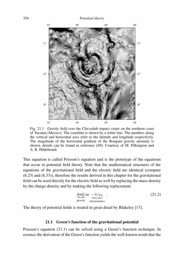
354 Potential theory
Fig. 21.1 Gravity field over the Chicxulub impact crater on the northern coastof Yucatan (Mexico). The coastline is shown by a white line. The numbers alongthe vertical and horizontal axes refer to the latitude and longitude respectively.The magnitude of the horizontal gradient of the Bouguer gravity anomaly isshown, details can be found in reference [49]. Courtesy of M. Pilkington andA. R. Hildebrand.
This equation is called Poisson’s equation and is the prototype of the equationsthat occur in potential field theory. Note that the mathematical structures of theequations of the gravitational field and the electric field are identical (compare(6.23) and (6.33)), therefore the results derived in this chapter for the gravitationalfield can be used directly for the electric field as well by replacing the mass-densityby the charge-density and by making the following replacement:
4πG︸︷︷︸
gravity
⇔ −1/ε0︸ ︷︷ ︸
electrostatics
. (21.2)
The theory of potential fields is treated in great detail by Blakeley [17].
21.1 Green’s function of the gravitational potential
Poisson’s equation (21.1) can be solved using a Green’s function technique. Inessence the derivation of the Green’s function yields the well-known result that the
21.1 Green’s function of the gravitational potential 355
gravitational potential for a point-mass m is given by −Gm/r . The use of Green’sfunctions was introduced in great detail in Chapter 18. The Green’s function G(r, r′)that describes the gravitational potential at location r generated by a point mass atlocation r′ satisfies the following differential equation:
∇2G(r, r′) = δ(
r − r′) . (21.3)
Take care not to confuse the Green’s function G(r, r′) with the gravitational cons-tant G.
Problem a Show that the solution of (21.1) is:
V (r) = 4πG∫
G(r, r′)ρ(r′) dV ′. (21.4)
Problem b The differential equation (21.3) has translational invariance, and isinvariant for rotations. Show that this implies that G(r, r′) = G(|r − r′|). Showby placing the point-mass at the origin by setting r′ = 0 that G(r ) satisfies
∇2G(r ) = δ (r) . (21.5)
Problem c Use the expression for the Laplacian in spherical coordinates to showthat for r > 0 (21.5) is given by
1
r2
∂
∂r
(
r2 ∂G(r )
∂r
)
= 0. (21.6)
Problem d Integrate this equation with respect to r to derive that the solution isgiven by G(r ) = A/r + B, where A and B are integration constants.
The constant B in the potential does not contribute to the forces that are associatedwith this potential because ∇ B = 0. For this reason the arbitrary constant B canbe taken to be equal to zero. The potential is therefore given by
G(r ) = A
r. (21.7)
Problem e The constant A can be found by integrating (21.5) over a sphere ofradius R centered around the origin. Show that Gauss’s theorem implies that∫ ∇2G(r )dV = ∮ ∇G · dS, use (21.7) in the right-hand side of this expressionand show that this gives A = −1/4π. Note that this result is independent ofthe radius R that you have used.
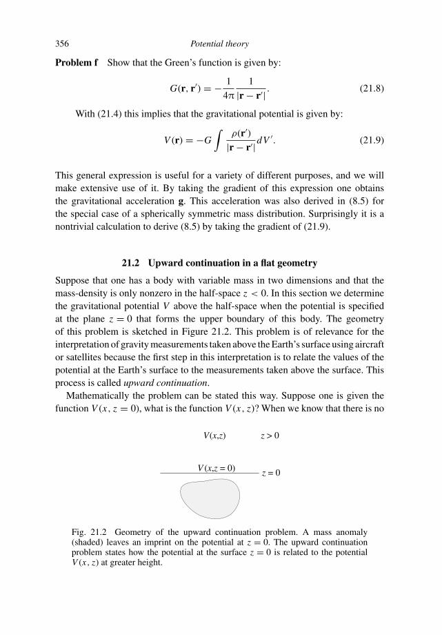
356 Potential theory
Problem f Show that the Green’s function is given by:
G(r, r′) = − 1
4π
1
|r − r′| . (21.8)
With (21.4) this implies that the gravitational potential is given by:
V (r) = −G∫
ρ(r′)|r − r′|dV ′. (21.9)
This general expression is useful for a variety of different purposes, and we willmake extensive use of it. By taking the gradient of this expression one obtainsthe gravitational acceleration g. This acceleration was also derived in (8.5) forthe special case of a spherically symmetric mass distribution. Surprisingly it is anontrivial calculation to derive (8.5) by taking the gradient of (21.9).
21.2 Upward continuation in a flat geometry
Suppose that one has a body with variable mass in two dimensions and that themass-density is only nonzero in the half-space z < 0. In this section we determinethe gravitational potential V above the half-space when the potential is specifiedat the plane z = 0 that forms the upper boundary of this body. The geometryof this problem is sketched in Figure 21.2. This problem is of relevance for theinterpretation of gravity measurements taken above the Earth’s surface using aircraftor satellites because the first step in this interpretation is to relate the values of thepotential at the Earth’s surface to the measurements taken above the surface. Thisprocess is called upward continuation.
Mathematically the problem can be stated this way. Suppose one is given thefunction V (x, z = 0), what is the function V (x, z)? When we know that there is no
V (x,z = 0) z = 0
z > 0V(x,z)
Fig. 21.2 Geometry of the upward continuation problem. A mass anomaly(shaded) leaves an imprint on the potential at z = 0. The upward continuationproblem states how the potential at the surface z = 0 is related to the potentialV (x, z) at greater height.
21.2 Upward continuation in a flat geometry 357
mass above the surface it follows from (21.1) that the potential satisfies:
∇2V (r) = 0 for z > 0. (21.10)
It is instructive to solve this problem by making a Fourier expansion of the potentialin the variable x :
V (x, z) =∫ ∞
−∞v(k, z)eikx dk. (21.11)
Problem a Show that for z = 0 the Fourier coefficients can be expressed in termsof the known value of the potential at the edge of the half-space:
v(k, z = 0) = 1
2π
∫ ∞
−∞V (x, z = 0)e−ikx dx . (21.12)
Problem b Use Poisson’s equation (21.10) and the Fourier expansion (21.11)to derive that the Fourier components of the potential satisfy for z > 0 thefollowing differential equation:
∂2v(k, z)
∂z2− k2v(k, z) = 0. (21.13)
Problem c Show that the general solution of this differential equation can bewritten as v(k, z) = A(k)e+|k|z + B(k)e−|k|z . The wave number k can be ei-ther positive or negative. By using the absolute value in the exponents it isexplicit that the solution consists of a superposition of an exponentially grow-ing solution (with z), and an exponentially decaying solution.
Since the potential must remain finite at great height (z → ∞) the coefficientA(k) must be equal to zero. Setting z = 0 shows that B(k) = v(k, z = 0), so thatthe potential is given by:
V (x, z) =∫ ∞
−∞v(k, z = 0)eikx e−|k|zdk. (21.14)
This expression is interesting because it states that the different Fourier componentsof the potential decay as e−|k|z with height.
Problem d Explain that this implies that the short-wavelength components in thepotential field decay faster with height than the long-wavelength components.
The decrease of the Fourier components with the distance z to the surface is prob-lematic when one wants to infer the mass-density in the body from measurements

358 Potential theory
of the potential or from gravity at a great height above the surface, because the in-fluence of mass perturbations on the gravitational field decays rapidly with height.The measurement of the short-wavelength component of the potential at a greatheight therefore carries virtually no information about the small-scale details of thedensity distribution within the Earth. This is the reason why gravity measurementsfrom space are preferably carried out using satellites in low orbits rather than inhigh orbits. Similarly, for gravity surveys at sea, a gravity meter has been devel-oped that is towed far below the sea surface [127]. The idea is that by towing thegravity meter closer to the sea bed, the gravity signal generated at the sub-surfacefor short wavelengths suffers less from the exponential decay due to upward con-tinuation.
Problem e Take the gradient of (21.14) to find the vertical component of thegravity field. Use the resulting expression to show that the gravity field g isless sensitive to the exponential decay due to upward continuation than thepotential V .
This last result is the reason why satellites in low orbits are used to measure theEarth’s gravitational potential and satellites in high orbits are used to measuregravity. In fact, a space-borne gradiometer [89] is presently being developed. Thisinstrument measures the gradient of the gravity vector by monitoring the differentialmotion between two masses in the satellite. Taking the gradient of the gravityleads to another factor of k in the Fourier expansion so that the effects of upwardcontinuation are further reduced.
We now explicitly express the potential at height z to the potential at the surfacez = 0.
Problem f Insert (21.12) into (21.14) to show that the upward continuation of thepotential is given by:
V (x, z) =∫ ∞
−∞H (x − x ′, z)V (x ′, z = 0) dx ′, (21.15)
with
H (x, z) = 1
2π
∫ ∞
−∞e−|k|zeikx dk. (21.16)
Note that (21.15) has exactly the same structure as (15.57) for a time-independentlinear filter. The only difference is that the variable x now plays the role of thevariable t in (15.57). This means that we can consider upward continuation as a

21.3 Upward continuation in a flat geometry in three dimensions 359
linear filtering operation. The convolutional filter H (x, z) maps the potential fromthe surface z = 0 onto the potential at height z.
Problem g Carry out the integral in expression (21.16) to show that this filter isgiven by:
H (x, z) = 1
π
z
z2 + x2. (21.17)
Problem h Sketch this filter as a function of x for a large value of z and a smallvalue of z.
Problem i Equation (21.15) implies that at the surface z = 0 this filter is givenby H (x, z = 0) = δ(x), with δ(x) the Dirac delta function. Convince yourselfof this by showing that H (x, z) becomes more and more peaked round x = 0when z → 0 and by proving that for all values of z the filter function satisfies∫∞−∞ H (x, z) dx = 1.
21.3 Upward continuation in a flat geometry in three dimensions
The analysis in the previous section is valid for a flat geometry in two dimensions.However, the theory can readily be extended to three dimensions by includinganother horizontal coordinate y in the derivation.
Problem a Show that the theory in the previous section up to equation (21.16)can be generalized by carrying out a Fourier transformation over both x andy. Show in particular that in three dimensions:
V (x, y, z) =∞∫∫
−∞H 3D(x − x ′, y − y′, z)V (x ′, y′, z = 0) dx ′dy′, (21.18)
with
H 3D(x, y, z) = 1
(2π)2
∞∫∫
−∞e−
√k2
x +k2y zei(kx x+ky y) dkx dky. (21.19)
The only difference with the case in two dimensions is that integral (21.19)leads to a different upward continuation filter than integral (21.16) for thetwo-dimensional case. The integral can be solved by switching the k-integral tocylindrical coordinates. The product kx x + ky y can be written as kr cos ϕ, where

360 Potential theory
k and r are the length of the k-vector and the position vector in the horizontalplane.
Problem b Use this to show that H 3D can be written as
H 3D(x, y, z) = 1
(2π)2
∫ ∞
0
∫ 2π
0ke−kzeikr cos ϕdϕdk. (21.20)
Note the factor k in the integrand.
Problem c As shown in Section 24.5, the Bessel function has the following inte-gral representation:
J0(x) = 1
2π
∫ 2π
0eix cos θdθ. (21.21)
Use this result to write the upward continuation filter as
H 3D(x, y, z) = 1
2π
∫ ∞
0e−kz J0(kr )kdk. (21.22)
It appears that we have only made the problem more complex, because theintegral of the Bessel function is not trivial. Fortunately, books and tables existwith a bewildering collection of integrals. For example, in equation (6.621.1) ofGradshteyn and Ryzhik [45] you can find an expression for the following integral:∫∞
0 e−αx Jν(βx)xµ−1dx .
Problem d What are the values of α, ν, β, and µ if we want to use this integralto solve the integration in (21.22)?
Take a look at the form of the integral in Gradshteyn and Ryzhik [45]. You willprobably be discouraged by what you find because the result is expressed in hyper-geometric functions, which means that you now have the new problem of findingout what these functions are. There is, however, a way out because (6.611.1) ofreference [45] gives the following integral:
∫ ∞
0e−αx Jν(βx) dx =
β−ν√
α2 + β2 − αν
√
α2 + β2. (21.23)
This is not quite the integral that we want because it does not contain a term thatcorresponds to the factor k in (21.22). However, we can introduce such a factor bydifferentiating (21.23) with respect to α.

21.4 Gravity field of the Earth 361
Problem e Do this to show that the upward continuation operator is given by
H 3D(x, y, z) = 1
2π
z(
x2 + y2 + z2)3/2 . (21.24)
Hint: you can make the problem simpler by first inserting the appropriate valueof ν in (21.23).
Problem f Compare the upward continuation operator (21.24) for three dimen-sions with the corresponding operator for two dimensions in (21.17). Which ofthese operators decays more rapidly as a function of the horizontal distance?Can you explain this difference physically?
Problem g In Section 21.2 you showed that the integral of the upward continu-ation operator over the horizontal distance is equal to 1. Show that the sameholds in three dimensions, that is show that
∫∫∞−∞ H 3D(x, y, z)dxdy = 1. The
integration simplifies by using cylindrical coordinates.
Comparing the upward continuation operators in different dimensions one findsthat these operators are different functions of the horizontal distance in the spacedomain. However, a comparison of (21.16) with (21.19) shows that in the wavenum-ber domain the upward continuation operators in two and three dimensions havethe same dependence on wave-number. The same is actually true for the Green’sfunction of the wave equation in one, two, or three dimensions. As you can see inSection 19.4 these Green’s functions are very different in the space domain, butone can show that in the wavenumber domain they are given in each dimension bythe same expression.
21.4 Gravity field of the Earth
In this section we obtain an expression for the gravitational potential outside theEarth for an arbitrary distribution of the mass density ρ(r) within the Earth. Thiscould be done be using the Green’s function that is appropriate for Poisson’s equa-tion (21.1). As an alternative we solve the problem here by expanding both themass-density and the potential in spherical harmonics and by using a Green’sfunction technique for every component in the spherical harmonics expansionseparately.
When using spherical harmonics, the natural coordinate system is a system ofspherical coordinates. For every value of the radius r both the density and the

362 Potential theory
potential can be expanded in spherical harmonics:
ρ(r, θ, ϕ) =∞∑
l=0
l∑
m=−l
ρlm(r )Ylm(θ, ϕ) (21.25)
and
V (r, θ, ϕ) =∞∑
l=0
l∑
m=−l
Vlm(r )Ylm(θ, ϕ). (21.26)
Problem a Use the orthogonality relation (20.50) of spherical harmonics to showthat the expansion coefficients for the density are given by:
ρlm(r ) =∫
Y ∗lm(θ, ϕ)ρ(r, θ, ϕ) dΩ, (21.27)
where∫
(· · ·) dΩ denotes an integration over the unit sphere.
Equation (21.1) for the gravitational potential contains the Laplacian. The Laplacianin spherical coordinates can be decomposed as
∇2 = 1
r2
∂
∂r
(
r2 ∂
∂r
)
+ 1
r2∇2
1, (21.28)
with ∇21 the Laplacian on the unit sphere:
∇21 = 1
sin θ
∂
∂θ
(
sin θ∂
∂θ
)
+ 1
sin2 θ
∂2
∂ϕ2. (20.34)
The reason why an expansion in spherical harmonics is used for the density andthe potential is that the spherical harmonics are the eigenfunctions of the operator∇2
1 (see (20.33) or p. 379 of Butkov [24]):
∇21Ylm = −l (l + 1) Ylm . (20.33)
Problem b Insert (21.25) and (21.26) into the Laplace equation, and use (20.33)and (20.34) for the Laplacian of the spherical harmonics to show that theexpansion coefficients Vlm(r ) of the potential satisfy the following differentialequation:
1
r2
∂
∂r
[
r2 ∂Vlm(r )
∂r
]
− l (l + 1)
r2Vlm(r ) = 4πGρlm(r ). (21.29)
21.4 Gravity field of the Earth 363
What we have gained by making the expansion in spherical harmonics is that(21.29) is an ordinary differential equation in the variable r whereas the originalequation (21.1) is a partial differential equation in the variables r , θ and ϕ. Thedifferential equation (21.29) can be solved using the Green’s function techniquedescribed in Section 18.3. Let us first consider a mass δ(r − r ′) located at a radiusr ′. The response to this mass is the Green’s function Gl that satisfies the followingdifferential equation:
1
r2
∂
∂r
[
r2 ∂Gl(r, r ′)∂r
]
− l (l + 1)
r2Gl(r, r ′) = δ
(
r − r ′) . (21.30)
Note that this equation depends on the angular order l but not on the angulardegree m. For this reason the Green’s function Gl(r, r ′) depends on l but noton m.
Problem c The Green’s function can be found by first solving the differentialequation (21.30) for r = r ′. Show that when r = r ′ the general solution of thedifferential equation (21.30) can be written as Gl = Arl + Br−(l+1), wherethe constants A and B do not depend on r .
Problem d In the regions r < r ′ and r > r ′ the constants A and B in general havedifferent values. Show that the requirement that the potential is everywherefinite implies that B = 0 for r < r ′ and that A = 0 for r > r ′. The solutioncan therefore be written as:
Gl(r, r ′) =
Arl for r < r ′
Br−(l+1) for r > r ′ . (21.31)
The integration constants follow in the same way as in the analysis of Section 18.3.One constraint on the integration constants follows from the requirement that theGreen’s function is continuous in the point r = r ′. The other constraint follows bymultiplying (21.30) by r2 and integrating the resulting equation over r from r ′ − ε
to r ′ + ε.
Problem e Show by taking the limit ε → 0 that this leads to the requirement
[
r2 ∂Gl(r, r′)
∂r
]r=r ′+ε
r=r ′−ε
= r ′2. (21.32)
364 Potential theory
Problem f Use this condition with the continuity of Gl to find the coefficients Aand B and show that the Green’s function is given by:
Gl(r, r ′) =
⎧
⎪
⎪
⎨
⎪
⎪
⎩
− 1
(2l + 1)
rl
r ′(l−1)for r < r ′
− 1
(2l + 1)
r ′(l+2)
r (l+1)for r > r ′
. (21.33)
Problem g Use this result to derive that the solution of (21.29) is:
Vlm(r ) = − 4πG
(2l + 1)
1
rl+1
∫ r
0ρlm(r ′)r ′(l+2)dr ′
− 4πG
(2l + 1)rl∫ ∞
rρlm(r ′)
1
r ′(l−2)dr ′. (21.34)
Hint: split the integration over r ′ into the interval 0 < r ′ < r and the intervalr ′ > r .
Problem h Let us now consider the potential outside the Earth. The radius of theEarth is denoted by the symbol a. Use the above expression to show that thepotential outside the Earth is given by
V (r, θ, ϕ) = −∞∑
l=0
l∑
m=−l
4πG
(2l + 1)
1
rl+1
∫ a
0ρlm(r ′)r ′(l+2)dr ′ Ylm(θ, ϕ). (21.35)
Problem i Eliminate ρlm using the result of problem a and show that the potentialis finally given by:
V (r, θ, ϕ) = −∞∑
l=0
l∑
m=−l
4πG
(2l + 1)
1
rl+1
×∫ a
0ρ(r ′, θ ′, ϕ′)r ′lY ∗
lm(θ′, ϕ′) dV ′ Ylm(θ, ϕ). (21.36)
Note that the integration in this expression is over the volume of the Earthrather than over the distance r ′ to the Earth’s center.
Let us reflect on the relation between this result and the derivation of upwardcontinuation in a Cartesian geometry of Section 21.2. Equation (21.36) can becompared with (21.14). In (21.14) the potential is written as an integration overwavenumber and the potential is expanded in basis functions eikx , whereas in (21.36)the potential is written as a summation over the degree l and order m and the potentialis expanded in basis functions Ylm . In both expressions the potential is written as

21.5 Dipoles, quadrupoles, and general relativity 365
a sum over basis functions with increasingly shorter wavelength as the summationindex l or the integration variable k increases. The decay of the potential withheight is in both geometries faster for a potential with rapid horizontal variationsthan for a potential with smooth horizontal variations. In both cases the potentialdecreases when the height z (or the radius r ) increases. In a flat geometry thepotential decreases as e−|k|z whereas in a spherical geometry the potential decreasesas r−(l+1). This difference in the reduction of the potential with distance is due tothe difference in the geometry in the two problems.
Expressions (21.9) and (21.36) both express the gravitational potential due tothe same density distribution ρ(r), therefore these expressions must be identical.
Problem j Use the equivalence of these expressions to derive that for r ′ < r thefollowing identity holds:
1
|r − r′| =∞∑
l=0
l∑
m=−l
4π
(2l + 1)Ylm(θ, ϕ)Y ∗
lm(θ′, ϕ′)
r ′l
r l+1. (21.37)
The derivation in this section could also have been made using (21.37) as a start-ing point because this expression can be derived by using the generating func-tion of Legendre polynomials and by using the addition theorem to obtain the m-summation [5, 53]. However, these concepts are not needed in the treatment in thissection which is based only on the expansion of functions in spherical harmonicsand on the use of Green’s functions.
As a last exercise let us consider the special case of a spherically symmetric massdistribution: ρ = ρ(r ). For such a mass distribution the potential is given by
V (r) = − G M
r, (21.38)
where M is the total mass of the body. The gradient of this potential is indeed equalto the gravitational acceleration given in (8.5) for a spherically symmetric mass M .
Problem i Derive the potential (21.38) from (21.36) by considering the specialcase that the mass-density depends only on the radius.
21.5 Dipoles, quadrupoles, and general relativity
We have seen in Section 8.2 that a spherically symmetric mass leads to a grav-itational field g(r) = −G M r/r2, which corresponds to a gravitational potentialV (r) = −G M/r . Similarly, the electric potential due to a spherically symmetriccharge distribution is given by V (r) = q/4πε0r , where q is the total charge. In this
366 Potential theory
section we investigate what happens if we place a positive charge and a negativecharge close together. Since there is no negative mass, we treat for the moment theelectric potential, but we will see in Section 21.6 that the results also have a bearingon the gravitational potential. The theory developed here is not only important inelectrostatics, it also accounts for the measurable effect of the ellipsoidal shapeof the Earth on its gravitational field. This application is treated in more detail inSection 21.7.
Consider a charge distribution that consists of a positive charge +q placed atposition a/2 and a negative charge −q placed at position −a/2 as shown in Figure21.3.
Problem a The total charge of this system is zero. What would you expect theelectric potential to be at positions that are very far from the charges comparedto the distance between the charges?
Problem b The potential follows by adding the potentials for the two pointcharges. Show that the electric potential generated by these two charges isgiven by
4πε0V (r) = q
|r − a/2| − q
|r + a/2| . (21.39)
Problem c Ultimately we will place the charges very close to the origin by takingthe limit a → 0. We can therefore restrict our attention to the special case thata r . Use a first order Taylor expansion to show that up to order a:
1
|r − a/2| = 1
r+ 1
2r3(r · a) . (21.40)
Hint: use that |r − a/2|−1 = [(r − a/2) · (r − a/2)]−1/2.
Problem d Insert this into (21.39) and derive that the electric potential is givenby:
4πε0V (r) = −q (r · a)
r3. (21.41)
Now suppose we bring the charges in Figure 21.3 closer and closer together, andsuppose we let the charge q increase so that the product p = qa is constant, thenthe electric potential is given by:
4πε0V (r) = − (r · p)
r2, (21.42)
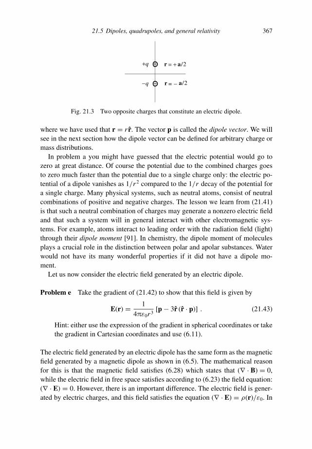
21.5 Dipoles, quadrupoles, and general relativity 367
+
−
+q
−q r
r = + a/2
a/2= −
Fig. 21.3 Two opposite charges that constitute an electric dipole.
where we have used that r = r r. The vector p is called the dipole vector. We willsee in the next section how the dipole vector can be defined for arbitrary charge ormass distributions.
In problem a you might have guessed that the electric potential would go tozero at great distance. Of course the potential due to the combined charges goesto zero much faster than the potential due to a single charge only: the electric po-tential of a dipole vanishes as 1/r2 compared to the 1/r decay of the potential fora single charge. Many physical systems, such as neutral atoms, consist of neutralcombinations of positive and negative charges. The lesson we learn from (21.41)is that such a neutral combination of charges may generate a nonzero electric fieldand that such a system will in general interact with other electromagnetic sys-tems. For example, atoms interact to leading order with the radiation field (light)through their dipole moment [91]. In chemistry, the dipole moment of moleculesplays a crucial role in the distinction between polar and apolar substances. Waterwould not have its many wonderful properties if it did not have a dipole mo-ment.
Let us now consider the electric field generated by an electric dipole.
Problem e Take the gradient of (21.42) to show that this field is given by
E(r) = 1
4πε0r3[p − 3r (r · p)] . (21.43)
Hint: either use the expression of the gradient in spherical coordinates or takethe gradient in Cartesian coordinates and use (6.11).
The electric field generated by an electric dipole has the same form as the magneticfield generated by a magnetic dipole as shown in (6.5). The mathematical reasonfor this is that the magnetic field satisfies (6.28) which states that (∇ · B) = 0,while the electric field in free space satisfies according to (6.23) the field equation:(∇ · E) = 0. However, there is an important difference. The electric field is gener-ated by electric charges, and this field satisfies the equation (∇ · E) = ρ(r)/ε0. In

368 Potential theory
+− −
+ −
+
+
monopole dipole quadrupole
Fig. 21.4 The definition of the monopole, dipole, and quadrupole in terms ofelectric charges.
the example in this section we created a dipole field by taking two opposite chargesand putting them closer and closer together. However, the magnetic field satisfies(∇ · B) = 0 everywhere. The reason for this is that the magnetic equivalent of theelectric charge, the magnetic monopole, has not been discovered in nature.
The fact that magnetic monopoles have not been observed in nature seems puz-zling, because we have seen that the magnetic dipole field has the same form asthe electric dipole field which was constructed by putting two opposite electriccharges close together. The reason for the analogy between an electric and a mag-netic dipole field is not that the magnetic dipole can be seen as a combination ofpositive and negative magnetic “charges” placed close together. In the context ofclassical electromagnetism, the magnetic dipole field is generated by a current thatruns in a small circular loop. On a microscopic scale a magnetic dipole is generatedby the spin of particles. This means that the electric and magnetic dipole fields havefundamentally different origins.
The starting point of the derivation in this section is the electric field of a singlepoint charge. Such a single point charge is called a monopole, see Figure 21.4. Thefield of this charge decays as 1/r2. If we put two opposite charges close togetherwe can create a dipole, see Figure 21.4. Its electric field is derived in (21.43); thisfield decays as 1/r3. We can also put two opposite dipoles together as shown inFigure 21.4. The resulting charge distribution is called a quadrupole. To leadingorder the electric fields of the dipoles that constitute the quadrupole cancel, and wewill see in the next section that the electric potential for a quadrupole decays as1/r3 so that the electric field decays with distance as 1/r4.
You may wonder whether the concept of a dipole or quadrupole can also beused for the gravity field because for the electric field these concepts are basedon the presence of both positive and negative charges whereas we know that onlypositive mass occurs in nature. However, there is nothing to keep us from comput-ing the gravitational field for a negative mass, and this is actually quite useful. Asan example, let us consider a double star that consists of two heavy stars whichrotate around their joint center of gravity. The first-order field is the monopole field

21.6 Multipole expansion 369
++ = ++ +−
+−
Fig. 21.5 The decomposition of a double star in a gravitational monopole and agravitational quadrupole.
that is generated by the joint mass of the stars. However, as shown in Figure 21.5the mass of the two stars can be seen as approximately the sum of a monopoleand a quadrupole consisting of two positive and two negative masses. Since thestars rotate, the gravitational quadrupole rotates as well, and this is the reasonwhy rotating double stars are seen as a prime source for the generation of gravi-tational waves [76]. However, gravitational waves that spread in space with timecannot be described by the classic expression (21.1) for the gravitational poten-tial.
Problem g Can you explain why (21.1) cannot account for propagating gravita-tional waves?
A proper description of gravitational waves depends on the general theory of rela-tivity [76]. Huge detectors for gravitational waves are being developed [8], becausethese waves can be used to investigate the theory of general relativity as well as theastronomical objects that generate gravitational waves.
21.6 Multipole expansion
Now that we have learned that the concepts of the monopole, dipole, and quadrupoleare relevant for both the electric field and the gravity field we continue the analysiswith the gravitational field. In this section we derive the multipole expansion inwhich the total field is written as a superposition of a monopole field, a dipole field,a quadrupole field, an octupole field, etc.
Consider the situation shown in Figure 21.6 in which a finite body has a mass-density ρ(r′). The gravitational potential generated by this mass is given by:
V (r) = −G∫
ρ(r′)|r − r′|dV ′. (21.9)
We consider the potential at a distance that is much larger than the size of the body.Since the integration variable r′ is limited by the size of the body, a “large distance”means in this context that r r ′. We therefore make a Taylor expansion of theterm 1/
∣
∣r − r′∣∣ in the parameter
(
r ′/r)
which is much smaller than unity.

370 Potential theory
r
r´
Fig. 21.6 Definition of the integration variable r′ within the mass and the obser-vation point r outside the mass.
Problem a Show that∣
∣r − r′∣∣ =
√
r2 − 2 (r · r′) + r ′2. (21.44)
Problem b Use a Taylor expansion in the small parameter r ′/r to show that:
1
|r − r′| = 1
r
1 + 1
r
(
r · r′)+ 1
2r2
[
3(
r · r′)2 − r ′2]
+ O
(
r ′
r
)3
. (21.45)
Be careful that you account for all the terms of order r ′ correctly. Alsobe aware of the distinction between the position vector r and the unitvector r.
From this point on we will ignore the terms of order(
r ′/r)3
.
Problem c Insert the expansion (21.45) into (21.9) and show that the gravitationalpotential can be written as a sum of different contributions:
V (r) = Vmon(r) + Vdip(r) + Vqua(r) + · · · , (21.46)
with
Vmon(r) = −G
r
∫
ρ(r′)dV ′, (21.47)
Vdip(r) = − G
r2
∫
ρ(r′)(
r · r′) dV ′, (21.48)
Vqua(r) = − G
2r3
∫
ρ(r′)[
3(
r · r′)2 − r ′2]
dV ′. (21.49)

21.6 Multipole expansion 371
It thus follows that the gravitational potential can be written as the sum of terms thatdecay with increasing powers of r−n . Let us analyze these terms in turn. The termVmon(r) in (21.47) is the simplest since the volume integral of the mass-density issimply the total mass of the body:
∫
ρ(r′)dV ′ = M . This means that this term isgiven by
Vmon(r) = −G M
r. (21.50)
This is the potential generated by a point mass M . To leading order, the gravitationalfield is the same as if all the mass of the body were concentrated in the origin. Themass distribution within the body does not affect this part of the gravitational fieldat all. Because the resulting field is the same as for a point mass, this field is calledthe monopole field.
For the analysis of the term Vdip(r) in (21.48) it is useful to define the center ofgravity rg of the body:
rg ≡∫
ρ(r′)r′dV ′∫
ρ(r′) dV ′ . (21.51)
This is simply a weighted average of the position vector with the mass-density asweight functions. Note that the word “weight” here has a double meaning!
Problem d Show that Vdip(r) is given by:
Vdip(r) = −G M
r2
(
r · rg)
. (21.52)
Note that this potential has exactly the same form as the potential (21.42) for anelectric dipole. For this reason Vdip(r) is called the dipole field.
Problem e Compared to the monopole term, the dipole term decays as 1/r2 ratherthan 1/r . The monopole term does not depend on r, the direction of obser-vation. Show that the dipole term varies with the direction of observation ascos θ and show how the angle θ must be defined.
Problem f You may be puzzled by the fact that the gravitational potential containsa dipole term, despite the fact that there is no negative mass. Draw a figuresimilar to Figure 21.5 to show that a displaced mass can be written as anundisplaced mass plus a mass dipole.

372 Potential theory
Of course, one is free in the choice of the origin of the coordinate system. If onechooses the origin to be at the center of mass of the body, then rg = 0 and the dipoleterm vanishes.
We now analyze the term Vqua(r) in (21.49). It can be seen from this expressionthat this term decays with distance as 1/r3. For this reason, this term is calledthe quadrupole field. The dependence of the quadrupole field on the direction ismore complex than for the monopole field and the dipole field. In the determinationof the directional dependence of the quadrupole term it is useful to use the doublecontraction between two tensors. Tensors are treated in Chapter 22. For the momentyou only need to know that the double contraction is defined as:
(A : B) ≡∑
i, j
Ai j Bi j . (21.53)
The double contraction generalizes the concept of the inner product of two vectors(a · b) =∑i ai bi to matrices or tensors of rank two. A double contraction occursfor example in the following identity
1 = (r · r) = (r · Ir) = (rr : I) , (21.54)
where I is the identity operator. Note that the term rr is a dyad. If you are unfamiliarwith the concept of a dyad you may want to look at Section 13.1 before continuingwith this chapter.
Problem g Use these results to show that Vqua(r) can be written as:
Vqua(r) = − G
2r3(rr : T) , (21.55)
where T is the inertia tensor defined as
T =∫
ρ(r)(
3rr − Ir2) dV . (21.56)
Note that we have renamed the integration variable r′ in the quadrupole mo-ment tensor as r.
Problem h Show that in explicit matrix notation T is given by:
T =∫
ρ(r)
⎛
⎝
2x2 − y2 − z2 3xy 3xz3xy 2y2 − x2 − z2 3yz3xz 3yz 2z2 − x2 − y2
⎞
⎠ dV . (21.57)
Note the resemblance between (21.55) and (21.52). For the dipole field the di-rectional dependence is described by the single contraction
(
r · rg)
whereas for
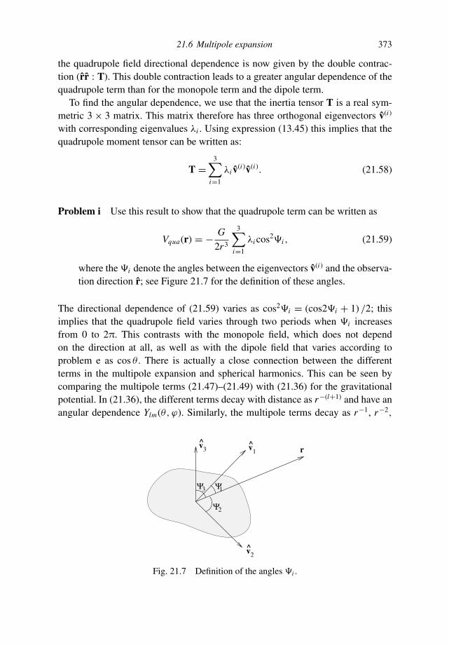
21.6 Multipole expansion 373
the quadrupole field directional dependence is now given by the double contrac-tion (rr : T). This double contraction leads to a greater angular dependence of thequadrupole term than for the monopole term and the dipole term.
To find the angular dependence, we use that the inertia tensor T is a real sym-metric 3 × 3 matrix. This matrix therefore has three orthogonal eigenvectors v(i)
with corresponding eigenvalues λi . Using expression (13.45) this implies that thequadrupole moment tensor can be written as:
T =3∑
i=1
λi v(i)v(i). (21.58)
Problem i Use this result to show that the quadrupole term can be written as
Vqua(r) = − G
2r3
3∑
i=1
λi cos2i , (21.59)
where the i denote the angles between the eigenvectors v(i) and the observa-tion direction r; see Figure 21.7 for the definition of these angles.
The directional dependence of (21.59) varies as cos2i = (cos2i + 1) /2; thisimplies that the quadrupole field varies through two periods when i increasesfrom 0 to 2π. This contrasts with the monopole field, which does not dependon the direction at all, as well as with the dipole field that varies according toproblem e as cos θ . There is actually a close connection between the differentterms in the multipole expansion and spherical harmonics. This can be seen bycomparing the multipole terms (21.47)–(21.49) with (21.36) for the gravitationalpotential. In (21.36), the different terms decay with distance as r−(l+1) and have anangular dependence Ylm(θ, ϕ). Similarly, the multipole terms decay as r−1, r−2,
^
v
v v r3 1
2
Ψ2
3Ψ Ψ1
Fig. 21.7 Definition of the angles i .
374 Potential theory
and r−3, respectively, and depend on the direction as cos 0, cos θ, and cos 2
respectively.
21.7 Quadrupole field of the Earth
Let us now investigate what the multipole expansion implies for the gravity field ofthe Earth. The monopole term is by far the dominant term. It explains why an applefalls from a tree, why the Moon orbits the Earth and most other manifestations ofgravity that we observe in daily life. The dipole term has in this context no physicalmeaning whatsoever. This can be seen from (21.52) which states that the dipoleterm only depends on the distance from the Earth’s center of gravity to the origin ofthe coordinate system. Since we are free in choosing the origin, the dipole term canbe made to vanish by choosing the origin of the coordinate system as the Earth’scenter of gravity. It is through the quadrupole field that some of the subtleties ofthe Earth’s gravity field become manifest.
Problem a The quadrupole field vanishes when the mass distribution in the Earthis spherically symmetric. Show this by computing the inertia tensor T whenρ = ρ(r ).
The dominant departure of the shape of the Earth from spherical is the flatteningof the Earth due to its rotation. If that is the case, then by symmetry one eigenvectorof T must be aligned with the Earth’s axis of rotation, and the two other eigenvectorsmust be perpendicular to the axis of rotation. By symmetry these other eigenvectorsmust correspond to equal eigenvalues. When we choose a coordinate system withthe z-axis along the Earth’s axis of rotation the eigenvectors are therefore givenby the unit vectors z, x, and y with eigenvalues λz , λx , and λy , respectively. Thelast two eigenvalues are identical because of the rotational symmetry around theEarth’s axis of rotation: hence λy = λx .
Let us first determine the eigenvalues. Once the eigenvalues are known, thequadrupole moment tensor follows from (21.59). The eigenvalues could be foundin the standard way by solving det (T−λI) = 0, but this is unnecessarily dif-ficult. Once we know the eigenvectors the eigenvalues can easily be foundfrom (21.58).
Problem b Take twice the inner product of (21.58) with the eigenvector v( j) toshow that
λ j = v( j) · T · v( j). (21.60)
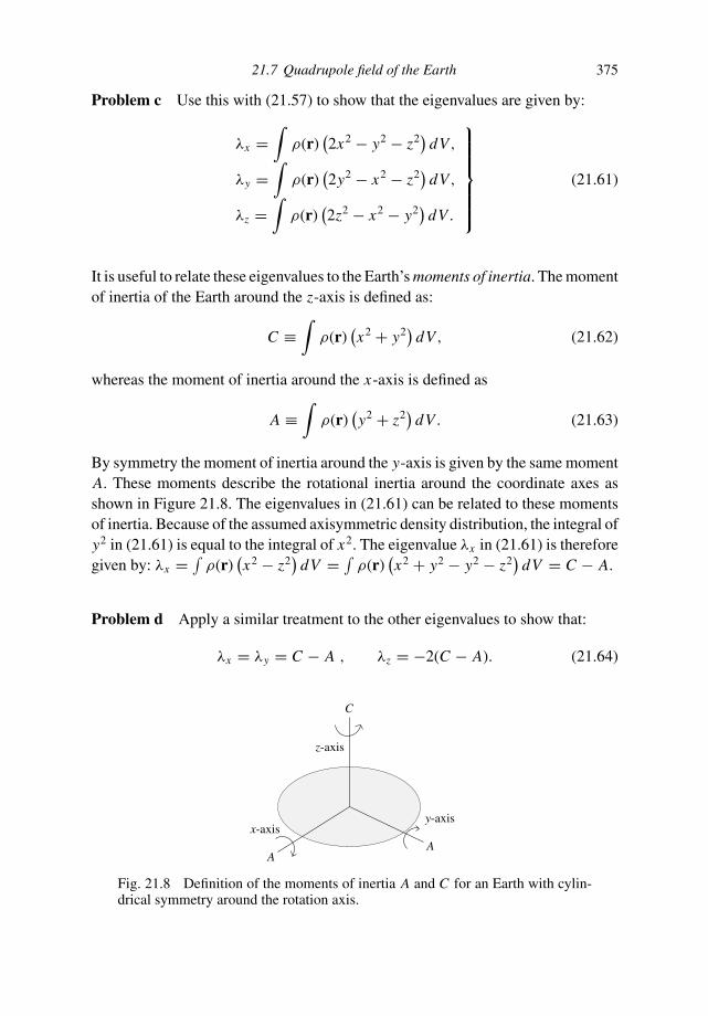
21.7 Quadrupole field of the Earth 375
Problem c Use this with (21.57) to show that the eigenvalues are given by:
λx =∫
ρ(r)(
2x2 − y2 − z2) dV,
λy =∫
ρ(r)(
2y2 − x2 − z2) dV,
λz =∫
ρ(r)(
2z2 − x2 − y2) dV .
⎫
⎪
⎪
⎪
⎪
⎪
⎬
⎪
⎪
⎪
⎪
⎪
⎭
(21.61)
It is useful to relate these eigenvalues to the Earth’s moments of inertia. The momentof inertia of the Earth around the z-axis is defined as:
C ≡∫
ρ(r)(
x2 + y2)
dV, (21.62)
whereas the moment of inertia around the x-axis is defined as
A ≡∫
ρ(r)(
y2 + z2) dV . (21.63)
By symmetry the moment of inertia around the y-axis is given by the same momentA. These moments describe the rotational inertia around the coordinate axes asshown in Figure 21.8. The eigenvalues in (21.61) can be related to these momentsof inertia. Because of the assumed axisymmetric density distribution, the integral ofy2 in (21.61) is equal to the integral of x2. The eigenvalue λx in (21.61) is thereforegiven by: λx = ∫ ρ(r)
(
x2 − z2)
dV = ∫ ρ(r)(
x2 + y2 − y2 − z2)
dV = C − A.
Problem d Apply a similar treatment to the other eigenvalues to show that:
λx = λy = C − A , λz = −2(C − A). (21.64)
A
C
x-axisA
y-axis
z-axis
Fig. 21.8 Definition of the moments of inertia A and C for an Earth with cylin-drical symmetry around the rotation axis.
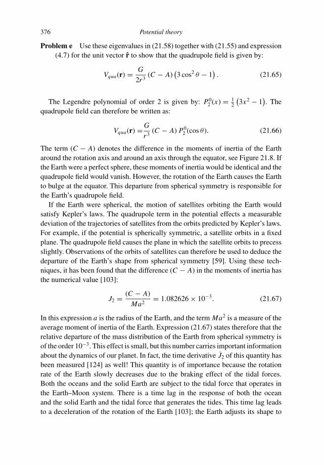
376 Potential theory
Problem e Use these eigenvalues in (21.58) together with (21.55) and expression(4.7) for the unit vector r to show that the quadrupole field is given by:
Vqua(r) = G
2r3(C − A)
(
3 cos2 θ − 1)
. (21.65)
The Legendre polynomial of order 2 is given by: P02 (x) = 1
2
(
3x2 − 1)
. Thequadrupole field can therefore be written as:
Vqua(r) = G
r3(C − A) P0
2 (cos θ ). (21.66)
The term (C − A) denotes the difference in the moments of inertia of the Eartharound the rotation axis and around an axis through the equator, see Figure 21.8. Ifthe Earth were a perfect sphere, these moments of inertia would be identical and thequadrupole field would vanish. However, the rotation of the Earth causes the Earthto bulge at the equator. This departure from spherical symmetry is responsible forthe Earth’s quadrupole field.
If the Earth were spherical, the motion of satellites orbiting the Earth wouldsatisfy Kepler’s laws. The quadrupole term in the potential effects a measurabledeviation of the trajectories of satellites from the orbits predicted by Kepler’s laws.For example, if the potential is spherically symmetric, a satellite orbits in a fixedplane. The quadrupole field causes the plane in which the satellite orbits to precessslightly. Observations of the orbits of satellites can therefore be used to deduce thedeparture of the Earth’s shape from spherical symmetry [59]. Using these tech-niques, it has been found that the difference (C − A) in the moments of inertia hasthe numerical value [103]:
J2 = (C − A)
Ma2= 1.082626 × 10⁻³. (21.67)
In this expression a is the radius of the Earth, and the term Ma2 is a measure of theaverage moment of inertia of the Earth. Expression (21.67) states therefore that therelative departure of the mass distribution of the Earth from spherical symmetry isof the order 10−3. This effect is small, but this number carries important informationabout the dynamics of our planet. In fact, the time derivative J2 of this quantity hasbeen measured [124] as well! This quantity is of importance because the rotationrate of the Earth slowly decreases due to the braking effect of the tidal forces.Both the oceans and the solid Earth are subject to the tidal force that operates inthe Earth–Moon system. There is a time lag in the response of both the oceanand the solid Earth and the tidal force that generates the tides. This time lag leadsto a deceleration of the rotation of the Earth [103]; the Earth adjusts its shape to

21.8 Fifth force 377
this deceleration. The measurement of J2 therefore provides important informationabout the response of the Earth to a time-dependent loading.
21.8 Fifth force
Gravity is the force in nature that was first understood by mankind through thediscovery by Newton of the law of gravitational attraction. The reason that thegravitational force was understood first is that this force manifests itself in themacroscopic world in the motion of the Sun, Moon, and planets. Later the electro-magnetic force, and the strong and weak interactions were discovered. This meansthat presently four forces are thought to be operative in nature. Of these four forces,the electromagnetic force and the weak nuclear force can now be described by asingle unified theory.
In the 1980s, geophysical measurements of gravity suggested that the gravita-tional field behaves in a different way over geophysical length scales (betweenmeters and kilometers) than over astronomical length scales (>104 km). This hasled to the speculation that this discrepancy is due to a fifth force in nature. Thisspeculation and the observations that fuelled this idea are clearly described byFishbach and Talmadge [41]. The central idea is that in Newton’s theory of gravitythe gravitational potential generated by a point mass M is given by (21.38):
VN (r) = −G M
r. (21.68)
The hypothesis of the fifth force presumes that a new potential should be added tothis Newtonian potential: this fifth potential is given by
V5(r) = −αG M
re−r/λ. (21.69)
Note that this potential has almost the same form as the Newtonian potential VN (r),the main differences are that the fifth force decays exponentially with distance overa length λ and that it is weaker than Newtonian gravity by a factor α. This ideawas prompted by measurements of gravity in mines, in the ice-cap of Greenland,on a 600 m high telecommunication tower, and by a number of other experimentalresults that seemed to disagree with the gravitational force that follows from theNewtonian potential VN (r).
Problem a Effectively, the fifth force leads to a change of the gravitational con-stant G with distance. Compute the gravitational acceleration g(r ) for thecombined potential VN + V5 by taking the gradient and write the result as

378 Potential theory
−G(r )M r/r2 to show that the effective gravitational constant is given by:
G(r ) = G[
1 + α(
1 + r
λ
)
e−r/λ]
. (21.70)
The fifth force thus effectively leads to a change of the gravitational constant over acharacteristic distance λ. This effect is small: in 1991 the value of α was estimatedto be less than 10−3 for all estimates of λ longer than 1 cm [41].
In doing geophysical measurements of gravity, one has to correct for perturbingeffects such as the topography of the Earth’s surface and density variations withinthe Earth’s crust. It has now been shown that the uncertainties in these correctionsare much larger than the observed discrepancy between the gravity measurementsand Newtonian gravity [80]. This means that the issue of the fifth force seems beclosed for the moment, and that the physical world appears again to be governedby four fundamental forces.
22
Cartesian tensors
In physics and mathematics, coordinate transformations play an important rolebecause many problems are much simpler when a suitable coordinate systemis used. Furthermore, the requirement that physical laws do not change undercertain transformations imposes constraints on the physical laws. An exampleof this is presented in Section 22.11 where it is shown that the fact that thepressure in a fluid is isotropic follows from the requirement that some physicallaws may not change under a rotation of the coordinate system. In this chapterit is shown how the change of vectors and matrices under coordinate transfor-mations is derived. The derived transformation properties can be generalized toother mathematical objects which are called tensors. In this chapter, only trans-formations of rectangular coordinate systems are considered. Since these coordi-nate systems are called Cartesian coordinate systems, the associated tensors arecalled Cartesian tensors. The transformation properties of tensors in Cartesian andcurvilinear coordinate systems are described in detail by Butkov [24] and Rileyet al. [87].
22.1 Coordinate transforms
In this section we consider the transformation of a coordinate system in two di-mensions. In Figure 22.1 an old coordinate system with coordinates xold and yold
is shown. The unit vectors along the old coordinate axis are denoted by ex,old andey,old . In a coordinate transformation, these old unit vectors are transformed to newunit vectors ex,new and ey,new, respectively. The matrix that maps the old unit vectorsonto the new unit vectors is denoted by C−1, hence
C−1ex,old = ex,new, C−1ey,old = ey,new. (22.1)
379

380 Cartesian tensors
ex,old^
ex,newe
y,new^
ey,old
xold
xnew
v
yold
ynew
Fig. 22.1 Definition of vectors in the original and transformed coordinatesystems.
The fact that we use the inverse of the matrix has no significance; the only reasonwe do so is that in the following sections we will mostly use the inverse of C−1
which is equal to C. The elements of the matrix C−1 are labeled as follows
C−1 =(
C−111 C−1
12
C−121 C−1
22
)
, (22.2)
where it is understood that C−1i j is not the inverse of the element Ci j , but is the
i, j-element of the matrix C−1.There is a close relation between the new basis vectors ex,new and ey,new and the
matrix C−1. To see this we first use that in the old coordinate system the unit vectorex,old is the unit vector in the x-direction and that ey,old is the unit vector in they-direction:
ex,old =(
10
)
, ey,old =(
01
)
. (22.3)
Problem a Let the matrix C−1 act on these expressions and use expression (22.1)to show that the first column of C−1 is given by ex,new while the second columnis equal to ey,new:
ex,new =(
C−111
C−121
)
, ey,new =(
C−112
C−122
)
. (22.4)

22.1 Coordinate transforms 381
Problem b Use (22.2) to show that this implies that the matrix C−1 can also bewritten as
C−1 = (
ex,new ey,new)
. (22.5)
In other words, the transformed basis vectors are the columns of the matrixthat describes the coordinate transform.
Let us now consider a vector v as shown in Figure 22.1. This vector is a phys-ical quantity that denotes, for example, the position of an object relative to somespecified origin. This vector is independent of any coordinate system since it is aphysical quantity. However, when we describe this vector we use a system of basisvectors to give the components of this vector in directions defined by the basisvectors. For example, using the old coordinate vectors ex,old and ey,old the vector vcan be decomposed into its components vold
x and voldy :
v =voldx ex,old + vold
y ey,old. (22.6)
This same vector can also be decomposed into its components along the new coor-dinate system
v =vnewx ex,new + vnew
y ey,new. (22.7)
The vector v is the same in each of these expressions. It is the goal of this section toderive the relation between the old components vold and the new components vnew.
Problem c Use that (22.6) and (22.7) are expressions for the same vector andinsert (22.3) and (22.4) for the unit vectors to show that the old and the newcomponents are related by
voldx
(
10
)
+ voldy
(
01
)
= vnewx
(
C−111
C−121
)
+ vnewy
(
C−112
C−122
)
. (22.8)
Problem d Rewrite this result to derive that
C−111 vnew
x + C−112 vnew
y = voldx ,
C−121 vnew
x + C−122 vnew
y = voldy .
(22.9)
At this point it is useful to introduce the vectors vold and vnew with the componentsof the vector in the old and new coordinate system respectively:
vold ≡(
voldx
voldy
)
, vnew ≡(
vnewx
vnewy
)
. (22.10)

382 Cartesian tensors
This harmless-looking definition belies a subtle complication. We now have threenotations for the same vector. The notation v denotes the physical vector that isdefined independently of any coordinate system, while the vectors vold and vnew
give the representation of this vector with respect to the old and the new coordinatesystems, respectively. It is crucial to separate these three different vectors.
Problem e Use the rules of matrix–vector multiplication to show that (22.9) im-plies that
C−1vnew = vold, (22.11)
and derive from this that
vnew = Cvold. (22.12)
This is the desired result because this expression prescribes how the old vectorvold is mapped in the coordinate transform onto the new vector vnew. It is interestingto compare this expression with (22.1) which states that the old unit vectors aremapped onto the new basis vectors by the inverse matrix C−1. There is a goodreason why the basis vectors transform with the inverse of the transformation matrixof the components. According to (22.6) the physical vector v is the product of thecomponents of the vector and the basis vectors: v =vx ex + vy ey . Since the physicalvector v by definition is not changed by the coordinate transform, the productvx ex + vy ey of the components and the basis vectors is invariant. This can onlybe the case when the transformation rule for the components is the inverse of thetransformation rule of the basis vectors.
The treatment in this section was for a two-dimensional coordinate transform.Each step of the argument can be generalized to coordinate transforms in more thantwo dimensions.
22.2 Unitary matrices
In the previous section, it was tacitly assumed that the matrix C was defined in sucha way that the new basis vectors ex,new and ey,new were of unit length. For a generalcoordinate transform C this is not true. We are, however, interested in orthonormalcoordinate systems only: these are coordinate systems in which the basis vectorshave unit length and are mutually orthogonal.
Problem a Let the unit vectors in a coordinate system be denoted by ei . Showthat for an orthonormal coordinate system
(
ei · e j) = δij, (22.13)

22.2 Unitary matrices 383
where δi j is the Kronecker delta which was defined in (11.15) as
δi j =
1 when i = j0 when i = j
(11.15)
When the old coordinate system and the new coordinate system are orthonormal,both coordinate systems must satisfy (22.13). The condition is certainly satisfiedwhen the inner product of two vectors does not change under the coordinate trans-formation. Such coordinate transformations are called unitary transformations. Tobe more specific, let u and v be two vectors in the old coordinate system that aremapped by the coordinate transform C to new vectors u′ = Cu and v′ = Cv, re-spectively. The coordinate transform C is called unitary when (u′ · v′) = (u · v), orequivalently
(Cu · Cv) = (u · v). (22.14)
Problem b Show that the fact that the length of a vector and the angle betweenvectors is preserved implies that the inner product of two vectors is preserved aswell. Examples of unitary coordinate transformations are rotations, reflectionsin a plane, or combinations of these. Draw a number of figures to convinceyourself that these coordinate transformations do not change the length of thevector and the angle between two vectors so that these transformations areindeed unitary.
Problem c The requirement (22.14) can be used to impose a constraint on C.Write the matrix products and the inner product in (22.14) in terms of thecomponents of the matrix C and the vectors u and v to derive that it is equivalentto
∑
i, j,k
Ci j u j Cikvk =∑
i
uivi . (22.15)
Writing out a matrix expression in its components has an important advantage.In general one cannot interchange the order of two matrices, because in general thematrix product AB differs from the matrix product BA.
Problem d Verify this statement by taking
A =⎛
⎝
0 1 0−1 0 00 0 1
⎞
⎠ and B =⎛
⎝
1 0 00 0 10 −1 0
⎞
⎠ (22.16)
and showing that AB = BA.
384 Cartesian tensors
Problem e Geometrically the matrix A represents a rotation around the z-axisthrough 90 degrees while B represents a rotation around the x-axis through90 degrees. Take this book and carry out these rotations in the two differentorders to see that the final orientation of the book is indeed different in eachcase.
This means that in general one cannot interchange the order of matrices in a product.However, when a term Ai j B jk occurs in a summation, the terms Ai j and B jk referto individual matrix elements. These matrix elements are regular numbers that canbe interchanged: Ai j B jk = B jk Ai j . This means that the decomposition of a matrixequation into its components allows us to move the individual components aroundin any way that we like.
In the following we will use the transpose CT of a matrix C extensively. This isthe matrix in which the rows and the columns are interchanged, so that
CTi j ≡ C ji . (22.17)
Problem f Use the results in this section to show that (22.15) can be written as∑
i, j,k
CTji Ciku jvk =
∑
i
uivi . (22.18)
At this point it is important to realize that it is immaterial how we label the summa-tion index. The right-hand side of (22.18) can just as well be written as
∑
j u jv j
because this sum and∑
i uivi both mean: “take the corresponding elements of uand v, multiply them and sum over all components.”
Problem g Show that (22.18) is equivalent to
∑
j,k
(
∑
i
CTji Cik
)
u jvk =∑
j
u jv j . (22.19)
Problem h Use the definition (11.15) of the Kronecker delta to show that∑
j u jv j = ∑
j,k δ jku jvk .
Problem i Use this result to show that C is unitary when it satisfies the followingcondition
(
∑
i
CTji Cik
)
= δ jk . (22.20)

22.3 Shear or dilatation? 385
At this point we use that δ jk is just the j,k element of the identity matrix I becausethe elements of this matrix are equal to 1 on the diagonal ( j = k) and equal to zerooff the diagonal ( j = k). In matrix notation, (22.20) for a unitary matrix thereforeimplies that
CT C = I. (22.21)
Problem j Show that this implies that the inverse of a unitary matrix is equal toits transpose:
C−1 = CT . (22.22)
This result can save you a lot of work. Suppose you need to invert a ma-trix, and suppose that you suspect that the matrix is unitary, then according to(22.22) the inverse matrix is equal to the transpose. You can verify whetherthis is indeed the case by multiplying this “guess” by the original matrix C tocheck whether the result is equal to the identity matrix; this amounts to applying(22.21).
Problem k The matrix corresponding to a rotation over an angle ϕ is given by
R =(
cos ϕ sin ϕ
− sin ϕ cos ϕ
)
. (22.23)
Compute the inverse of this matrix with a minimal amount of work. (This isalso called the principle of maximal laziness.)
22.3 Shear or dilatation?
As an example of the importance of coordinate transforms we consider a geologistwho observes a rock sample that is subjected to a shear as shown in Figure 22.2.The height and the width of the rock are of unit length. In the shear motion theupper side of the rock is displaced rightward over a distance d while the lower sideof the rock is displaced leftward over a distance −d.
Problem a Use Figure 22.2 to show that the original unit vectors change duringthe deformation as
(
10
)
→(
10
)
and
(
01
)
→(
d1
)
. (22.24)

386 Cartesian tensors
d
x
y
Fig. 22.2 The shear of a rock as seen by the geologist before (dashed lines) andafter (solid lines) the shear.
Problem b Let the deformation be described by a 2 × 2 matrix D. Show that thismatrix is given by
D =(
1 d0 1
)
. (22.25)
Hint: check that this produces the deformation described by (22.24).
The geologist is in general interested in the internal deformation of the rock.However, the transformation shown in Figure 22.2 entails both a deformation withinthe rock sample as well as a rotation of the sample. We first need to unravel thesetwo contributions. In the following we only considered very small shear (d 1),the associated rotation is therefore also small.
Problem c Use a Taylor expansion of (22.23) to show that the rotation matrixover an infinitesimal angle ϕ is given by
R = I +(
0 ϕ
−ϕ 0
)
. (22.26)
The shear described by (22.25) can be decomposed into this rotation plus an internaldeformation. To make this explicit we decompose the matrix D into the matrix onthe right-hand side of (22.26) which accounts for the rotation and a new matrix E:
D =(
0 ϕ
−ϕ 0
)
+ E. (22.27)

22.3 Shear or dilatation? 387
At this point we need to find the parameter ϕ that characterizes the rotationalcomponent. It follows from (22.26) that the difference between the 12-componentand the 21-component of the matrix is equal to 2ϕ. According to (22.25) thisdifference is given by D12 − D21 = d; since this is equal to 2ϕ the rotation angleis given by ϕ = d/2.
Problem d Use the expressions (22.25), (22.27), and the relation ϕ = d/2 toshow that the deformation component of the transformation in Figure 22.2 isgiven by
E =(
1 d/2d/2 1
)
. (22.28)
Note that this matrix is symmetric(
Ei j = E ji)
, whereas the matrix R in (22.26)is antisymmetric
(
Ri j = −R ji)
. The matrix D has thus been decomposed intoa symmetric part and an antisymmetric part. This corresponds to a decomposi-tion of the deformation into a rotational component plus a deformation. We haveseen this before in Chapter 7 where it was shown that the curl of a vector fieldin general has two contributions: rotation and shear. We return to this issue inSection 22.9.
Problem e We now focus on the internal deformation of the sample. Show thatFigure 22.3 displays the deformation E of the rock. Hint: determine first whathappens to the unit vectors in the x- and y-directions when they are multipliedwith the matrix E.
x
y
d/2
Fig. 22.3 The same deformation as in the previous figure when the rotationalcomponent is removed. The undeformed sample is shown by the dashed lines, thedeformed sample by the solid lines.
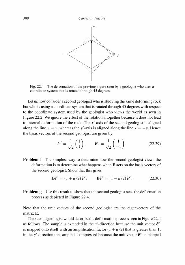
388 Cartesian tensors
x′
y′
Fig. 22.4 The deformation of the previous figure seen by a geologist who uses acoordinate system that is rotated through 45 degrees.
Let us now consider a second geologist who is studying the same deforming rockbut who is using a coordinate system that is rotated through 45 degrees with respectto the coordinate system used by the geologist who views the world as seen inFigure 22.2. We ignore the effect of the rotation altogether because it does not leadto internal deformation of the rock. The x ′-axis of the second geologist is alignedalong the line x = y, whereas the y′-axis is aligned along the line x = −y. Hencethe basis vectors of the second geologist are given by
ex ′ = 1√2
(
11
)
, ey′ = 1√2
(
1−1
)
. (22.29)
Problem f The simplest way to determine how the second geologist views thedeformation is to determine what happens when E acts on the basis vectors ofthe second geologist. Show that this gives
Eex ′ = (1 + d/2) ex ′, Eey′ = (1 − d/2) ey′
. (22.30)
Problem g Use this result to show that the second geologist sees the deformationprocess as depicted in Figure 22.4.
Note that the unit vectors of the second geologist are the eigenvectors of thematrix E.
The second geologist would describe the deformation process seen in Figure 22.4as follows. The sample is extended in the x ′-direction because the unit vector ex ′
is mapped onto itself with an amplification factor (1 + d/2) that is greater than 1;in the y′-direction the sample is compressed because the unit vector ey′
is mapped

22.4 Summation convention 389
onto itself with an amplification factor (1 − d/2) that is smaller than 1. This meansthat (apart from a rotation) the first geologist describes the transformation as pureshear whereas the second geologist describes the transformation as a combination ofextension and compression. These two points of view must be equivalent. However,they can be reconciled only when we have techniques for switching from onecoordinate system to another. This is the goal of tensor calculus. Before we derivethe transformation rules for matrices and more general tensors, we first introducea notational convention that turns out to be very convenient.
22.4 Summation convention
In this section the summation convention is introduced; this convention is some-times also referred to as the “Einstein summation convention.” Let us consider themultiplication of the matrix A by a vector x that gives a new vector y = Ax.
Problem a This is a vectorial notation; show that in component form this expres-sion should be written as
∑
j
Ai j x j = yi . (22.31)
You have seen in Section 22.2 that in matrix and vector calculations one has tocarry out a lot of summations. It is also shown in that section that working with theexpressions in component form has advantages over working with the more abstractvector/matrix notation. We could save a lot of work by leaving out the summationsigns in the equations. This is exactly what the summation convention does:
In the summation convention one leaves out the summation signs(∑)
with the understanding that one sums over any repeated index on eitherside of the equation.
What does this mean for expression (22.31)? In this expression we sum over theindex j . Note that this index appears twice on the left-hand side. According to thesummation convention we would write this expression as
Ai j x j = yi . (22.32)
It takes some time to get used to this notation. It should be kept in mind that underthe summation convention the identity (22.32) does not imply that this expressionholds for a single value of j . For example, (22.32) does not mean that Ai2x2 = yi
because a summation over the index j is implied rather than that j can take anyfixed value j = 1 or j = 2 or j = 3.
390 Cartesian tensors
As another example of the summation convention consider the inner productof two vectors. Normally one would write this as (u · v) = ∑
i uivi ; using thesummation convention one writes it as (u · v) = uivi . Note that the name of thesummation index is irrelevant. This expression could therefore also be writtenas (u · v) = u jv j . The matrix equation CT C = I is written in component formas
∑
k CTikCkj = ∑
k CikCkj = δi j ; in the summation convention this is written asCT
ikCkj = CikCkj = δi j .
Problem b Write out the matrix product AI (with I as the identity matrix) incomponent form, and show that the result can be written as: (AI)i j = Aikδk j .
In the last term a summation over the index k is implied. The Kronecker delta isalways zero, except when k = j . This means that the only nonzero contributionfrom the k-summation comes from the term k = j , so that (AI)i j = Aikδk j = Ai j .This is simply the identity AI = A in component form.
Problem c Show that v2 = vivi where v is the length of the vector v.
Problem d The Laplacian is the divergence of the gradient, use this to write theLaplacian in the following form
∇2 f = ∂i∂i f, (22.33)
with ∂i ≡ ∂/∂xi .
Problem e Use the summation convention to rewrite expression (11.55) as
∂(ρvi )
∂t+ ∂ j (ρv jvi ) = µ∂k∂kvi + Fi . (22.34)
Problem f In some applications one carries out summations over several indices.As an example consider the double sum
∑
i, j Ai jδ j i . Carry out the summationand show that the result can be written as
Ai jδ j i = Aii . (22.35)
Note that on the left-hand side a summation over i and j is implied whereas on theright-hand side a sum over i is implied. The term on the right-hand side is the sumof the diagonal elements of the matrix A. This quantity plays an important role ina variety of applications and is called the trace of A:
tr A ≡∑
i
Aii = Aii . (22.36)
22.5 Matrices and coordinate transforms 391
One caveat should be made with the summation convention. Suppose that onewrites Mii = 0. According to the summation convention this means that the traceof M is equal to zero. However, one could also mean to express that all the di-agonal elements of M are equal to zero: M11 = M22 = M33 = 0. This is an ex-ample where an expression can be ambiguous. It is important to state explicitlywhether one uses the summation convention. When one does, one can indicatethat one deviates from this convention in an equation by explicitly stating that nosummation is implied. For example, when one wants to express that all the di-agonal elements of M are equal to zero one could write this in the summationconvention as:
Mii = 0 (no summation over i). (22.37)
Problem g Use the properties of unitary matrices as derived in Section 22.2 toshow that for a unitary matrix C:
Ci j Cik = δk j . (22.38)
22.5 Matrices and coordinate transforms
In this section we determine the transformation properties of matrices under acoordinate transform C as introduced in Section 22.1. In the remainder of thissection we then restrict ourselves to unitary coordinate transformations. Let a matrixD map a vector x to a vector y
y = Dx. (22.39)
Consider this same operation in a new coordinate system and let us use a primeto denote the corresponding quantities is the new coordinate system. According to(22.12) the vector x in the new coordinate system is given by x′ = Cx, and a similarexpression holds for y. Expression (22.39) is given in the new coordinate systemby
y′= D′x′. (22.40)
In this section we determine the relation between the matrix D′ in the new coordinatesystem and the old matrix D.
Problem a Use (22.12) to show that (22.40) can be written as
Cy = D′Cx. (22.41)

392 Cartesian tensors
Problem b Multiply this expression on the left by C−1, compare the result with(22.39) to derive that D = C−1D′C. Multiply this last expression on the leftand the right by suitable matrices to derive that
D′ = CDC−1. (22.42)
This is the general transformation rule for matrices under a coordinate transform.It looks different from the transformation rule (22.12) for vectors because in (22.42)the inverse C−1of the coordinate transformation appears as well. However, forunitary coordinate transforms one can eliminate this inverse and write (22.42) in away that is similar to (22.12).
Problem c Use that C is unitary and rewrite (22.42) in component form as
D′i j =
∑
k,l
CikC jl Dkl . (22.43)
(Remember that you cannot interchange the order of matrices in a mul-tiplication, but that you can change the order of matrix elements that aremultiplied.)
Problem d Redo the calculation in the last problem using the summation con-vention at every step and rewrite the preceding result as
D′i j = CikC jl Dkl . (22.44)
Problem e To compare this result with the transformation rule (22.12) for vectorswrite vold = v, vnew = v′ and use the summation convention to rewrite (22.12)using the summation convention as
v′i = Ci jv j . (22.45)
Applying the matrix transformation (22.44) may appear to be complex to you.The easiest way to apply it in practice is to write it as
D′ = CDCT . (22.46)
This expression is identical to (22.42) with the only exception that it uses that C isunitary: C−1 = CT .

22.6 Definition of a tensor 393
Problem f According to (22.23) a rotation through 45 degrees of the coordinatesystem is described by the coordinate transform
C = 1√2
(
1 1−1 1
)
. (22.47)
Check that this coordinate transformation transforms the matrix E in (22.28)to the matrix
E′ =(
1 + d/2 00 1 − d/2
)
. (22.48)
Show also that this matrix describes the deformation shown in Figure 22.4.
22.6 Definition of a tensor
Expressions (22.44) and (22.45) allow us to see a resemblance between the trans-formation rule (22.44) for a matrix and the rule (22.45) for a vector. In bothequations the old vector or matrix is multiplied by the matrix C; for the vec-tor this happens once and for the matrix it happens twice. The first index ofthe quantity on the left-hand side (i in both cases) is the first index of the firstmatrix C on the right-hand side as indicated by the arrows in the followingexpressions:
v′i⇑
= Ci⇑
jv j , D′i⇑
j = Ci⇑
kC jl Dkl .
The second index of D′in (22.44) corresponds to the first index of the second term
C as indicated by the arrows:
D′i j⇑
= CikC j⇑
l Dkl .
In both (22.44) and (22.45) the second index of each term C also occurs in theterm D or v on which this matrix acts as shown by the arrows in the followingexpressions:
v′i = Ci j
⇑v j
⇑, D
′i j = Cik
⇑C jl Dk
⇑l, D
′i j = CikC j l
⇑Dk l
⇑.
Note that according to the summation convention, a summation over these repeatedindices is implied.
Some quantities that we use are not labeled by any index. Examples are tempera-ture and pressure. Such a quantity is a pure number and it is called a scalar. A vectorhas a direction and is labeled with one index and a matrix has two indices. There

394 Cartesian tensors
is no reason not to define objects which are characterized with an arbitrary numberof indices. In general a physical quantity can have any number of subscripts, and aquantity with n subscripts can be denoted as Ti1i2···in . We call such an object a tensorwhen it follows a transformation rule similar to (22.44) and (22.45) for a matrixand a vector, respectively.
Definition The quantity Ti1i2···in is called a tensor of rank n when it transformsunder a unitary coordinate transform C with the following transformation rule:
T ′i1i2···in
= Ci1 j1Ci2 j2 · · · Cin jn Tj1 j2··· jn . (22.49)
Note that the summation convention is used so a summation over the indicesj1, j2, . . . , jn is implied.
Problem a Convince yourself that the transformation rules (22.44) and (22.45)for a matrix and a vector, respectively, are special cases of this definition forthe values n = 2 and n = 1, respectively.
This means that a vector that transforms according to (22.45) is a tensor of rank oneand a matrix that transforms according to (22.44) is a tensor of rank two. Note thata scalar does not change under coordinate transformations. It has zero subscriptsand one can say that when one applies the coordinate transformation (22.49) thecoordinate transform C is applied zero times, for this reason one calls a scalar atensor of rank zero.
Let us consider some examples of tensors. The position vector r is a tensor ofrank one, as follows from the transformation rule (22.12) that you derived in Section22.1. From this it follows that the velocity vector v is a tensor of rank one providedthat the coordinate transformation C does not depend on time.
Problem b Differentiate the transformation law x′i = Ci j x j for the position vec-
tor with respect to time and use the result to show that the velocity indeedtransforms as a tensor of rank one.
Problem c Show that acceleration is a tensor of rank one.
Now we can use Newton’s law F = ma and that the mass m is a scalar. Since theacceleration is a tensor of rank one, the force must also be a tensor of rank one.

22.6 Definition of a tensor 395
It is interesting to see what happens when one works in a rotating coordinatesystem. In that case the transformation C which transforms the fixed system to therotating system depends on time.
Problem d Go through the steps of problems b and c and show that in that casethe acceleration transforms as
a′i = Ci j a j + 2Ci jv j + Ci j x j , (22.50)
where the dot denotes a time derivative.
This means that for such a time-dependent coordinate transform the accelerationdoes not transform as a vector of rank one. Note that additional terms appear thatare proportional to the velocity and the position vector. These correspond to theCoriolis force and the centrifugal force as treated in Section 13.3.
Another example of a tensor of rank one is the gradient vector ∇ i = ∂/∂xi . Thechain rule of differentiation states that
∇′i = ∂
∂x ′i
= ∂x j
∂x ′i
∂
∂x j= ∂x j
∂x ′i
∇ j , (22.51)
where to conform with the summation convention a summation over j is implied.
Problem e Use the transformation law of the position vector to derive that∂x j/∂x ′
i = C−1j i , and use the property that C is a unitary matrix to derive
that
∇′i = Ci j∇ j . (22.52)
In other words, the gradient vector is a tensor of rank one.
As an example of a tensor of rank two we consider the identity matrix whoseelements are the Kronecker delta δi j . At first sight you might believe that sincethe elements of the Kronecker delta are simply equal to zero or one, it is a scalar.However, the identity matrix really transforms like a tensor of rank two.
Problem f To see this, assume that the identity matrix follows the transformationrule (22.44) and use the property of the Kronecker delta to derive that
I ′i j = CikC jlδkl = CikC jk . (22.53)

396 Cartesian tensors
Problem g Write the last term as CTkj and use the property that C is unitary to
derive that
I ′i j = δi j . (22.54)
In other words, the identity matrix transforms as a tensor of rank two and yet ittakes the same form in every coordinate system!
22.7 Not every vector is a tensor
At this point you may think that any object with n-components is a tensor of rankone. However, keep in mind that not every vector transforms according to thetransformation rule (22.49) for a tensor. Let us first consider an obvious example.One might be interested in the distribution of shoe sizes of students. In such a studyone would measure the shoe size of each student in the group and could form avector of the data that one obtains:
d ≡
⎛
⎜
⎜
⎜
⎝
shoe size of Marieshoe size of Petershoe size of Klaas
...
⎞
⎟
⎟
⎟
⎠
. (22.55)
This vector is not a tensor. There are two reasons for this. The coordinate trans-formation matrix C is by definition a square matrix with a dimension equal to thedimension of the coordinate system (usually 3 and for some applications 4, seeSection 22.12). The vector d can have any dimension and the action of C in thisvector is not defined. The second reason why d is not a tensor of rank one is thatthe shoe size of students does not depend on the coordinate system. In other words,all the elements of d are scalars, hence d is certainly not a tensor of rank one.
Another example of a vector that is not a tensor is the stress–displacement tensorthat is used in the description of elastic wave propagation in elastic media [3]:
w =(
uy
σ yz
)
, (22.56)
where uy and σ yz are suitably chosen components of the displacement and thestress. This vector is not a tensor of rank one. It has a different dimension than C,hence the action of C on this vector is not defined. Furthermore the components ofw are of different dimension, hence they can never be mixed in the transformationrule (22.49).
Let us now consider a more subtle example. At this point you might think thatthe magnetic field vector is a tensor of rank one. Consider the circular current in

22.7 Not every vector is a tensor 397
I
x
y
z
B
B
Q
P
Fig. 22.5 A circular current that generates a magentic field B.
the (x, y)-plane shown in Figure 22.5 that generates a magnetic field. Given thedirection of this current the magnetic field on the z-axis is oriented in the directionof the positive z-axis. This holds for the points P and Q in Figure 22.5.
Problem a Let us perform the coordinate transformation in which the system isreflected in the (x, y)-plane. Make a drawing of the transformed current andmake sure you understand that the current has not changed in the coordinatetransform.
Problem b Now that you know that the current has not changed, use Figure 22.5to draw the associated magnetic field vector at the points P and Q.
Problem c Now add to your figure the image of the vectors B of Figure 22.5 afterthey have been subjected to a reflection in the (x, y)-plane.
If you made the drawing correctly, you will have found that the magnetic field thatyou obtained after transforming the original magnetic field vector had the oppositedirection to the magnetic field that was generated by the current that had beensubjected to the coordinate transform.
The only conclusion is that the magnetic field does not behave like a tensorof rank one under coordinate transforms: it does not transform according to thetransformation rule (22.45). In fact, the magnetic field behaves in a different way. It
398 Cartesian tensors
is an example of a pseudo-tensor indicating that it shares some of the properties ofthe tensors that we have explored, but that its transformation rules differ from thetransformation rule (22.45) that we have been used to. More details about pseudo-tensors can be found in reference [87]. The main thing to remember at this point isthat not every vector is a tensor!
The next example shows that not every tensor is Cartesian. In Section 4.2 wederived the transformation that maps the components vx , vy , and vz of a vector inCartesian coordinates into its components vr , vθ , and vϕ in spherical coordinates:
⎛
⎝
vr
vθ
vϕ
⎞
⎠ =⎛
⎝
sin θ cos ϕ sin θ sin ϕ cos θ
cos θ cos ϕ cos θ sin ϕ − sin θ
− sin ϕ cos ϕ 0
⎞
⎠
⎛
⎝
vx
vy
vz
⎞
⎠ . (4.19)
This transformation is of the same form as the general transformation rule (22.45)for a tensor of rank one. However, the matrix of the coordinate transform nowdepends on the position; this is a result of the fact that the spherical coordinatesystem is curvilinear. When we take a derivative of the vector, the dependence ofthe transformation matrix on the position gives additional terms. For this reasontensor calculus for tensors in curvilinear coordinate systems is significantly morecomplex than tensor calculus for Cartesian tensors.
22.8 Products of tensors
One can form products of vectors in different ways. You have probably seen theinner product and outer product of vectors. There are also other ways in whichone can make products of tensors. The first product of tensors that we consider isthe contraction. You have already seen examples of this: the inner product of twovectors is one:
(u · v) = uivi . (22.57)
Another example is matrix–vector multiplication:
(M · v)i = Mi jv j . (22.58)
Note that according to the summation convention a summation over i is implied in(22.57) and a summation over j in (22.58).
These operations can be extended. Let Ui1i2···in be a tensor of rank n and Vj1, j2··· jm
a tensor of rank m. The contraction of U and V is defined by setting the last indexof U equal to the first index of V and summing over this index:
(U · V)i1i2···in−1k2···km= Ui1···in−1r Vrk2···km . (22.59)
Note that we sum over the index r .
22.8 Products of tensors 399
Problem a Show that the rank of this tensor is n + m − 2.
Problem b Show that the inner product of two vectors and matrix-vector multi-plication are special cases of the contraction (22.59). Make sure you define nand m in each example. Verify that the rank of the result is indeed n + m − 2.
One can also apply a multiple contraction in which one sums over two or moreindices of the tensors that one contracts. For example, the double contraction isgiven by
(U : V)i1i2···in−2k3···km= Ui1···in−2rs Vsrk3···km . (22.60)
Problem c Show that the resulting tensor is of rank n + m − 4.
A very important property is that the contraction of two tensors is also a tensor.The proof of this property is not difficult, it is mostly a tedious bookkeeping exercise,and the details can be found for example in references [24] and [87]. Here we willstudy some examples.
Problem d Show that the double contraction of a matrix A with the identity matrixis equal to the trace of A as defined in (22.36):
(A : I) = Aii = tr A. (22.61)
The fact that the contraction of a tensor is also a tensor implies that the trace of amatrix is a tensor of rank zero: the trace of a matrix is a scalar. Therefore the traceof a matrix is invariant to unitary coordinate transformations.
Problem e There is one coordinate transformation in which the new basis vectorsare aligned with the eigenvectors of A. Show that in that particular coordinatesystem the trace is equal to the sum of the eigenvectors λi . Use this result toderive that in any coordinate system the trace of a matrix is equal to the sumof the eigenvalues:
tr A =∑
i
λi . (22.62)
A matrix that is often used is the Hessian of a function f which is defined bythe second partial derivatives of that function:
Hi j ≡ ∂2 f
∂xi∂x j. (22.63)
400 Cartesian tensors
Problem e Show that H is a tensor of rank two by generalizing the derivationof problem e of Section 22.6 to the transformation properties of the secondderivative.
Problem f Show that the trace of the Hessian is the Laplacian of f
tr H = ∇2 f. (22.64)
The trace is invariant for unitary coordinate transformations and the Laplacian isthe trace of a tensor; therefore the Laplacian is invariant for unitary coordinatetransformations as well.
The second type of product of tensors is the direct product. The direct productof two tensors is formed by multiplying the different elements of the two tensorswithout carrying out a summation over repeated indices. An example of this isthe dyad of two vectors that you encountered for example in Section 13.1 wherethe projection operator is written as the direct product of the unit vector n withitself:
P = nnT . (13.5)
In component form this expression is given by
Pi j = ni n j . (22.65)
This idea can be generalized to form the direct product of a tensor U of rank n anda tensor V of rank m. This direct product is usually denoted with the symbol ⊗:
(U ⊗ V)i1···in j1··· jm = Ui1···in Vj1··· jm . (22.66)
Note that there are no repeated indices over which one sums.
Problem g Show that the rank of this direct product is n + m.
Problem h Show that the dyad (13.5) is a special example of the direct product(22.65).
Problem i The direct product of two tensors is also a tensor. Show this propertyby applying the transformation rule (22.49) to the tensors on the right-handside of (22.66).
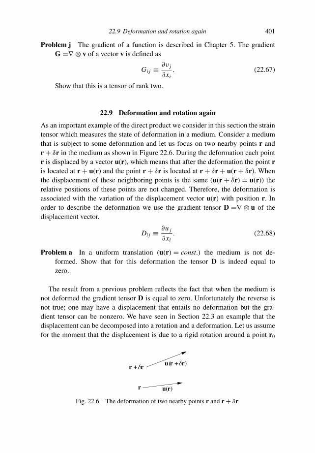
22.9 Deformation and rotation again 401
Problem j The gradient of a function is described in Chapter 5. The gradientG =∇ ⊗ v of a vector v is defined as
Gi j ≡ ∂v j
∂xi. (22.67)
Show that this is a tensor of rank two.
22.9 Deformation and rotation again
As an important example of the direct product we consider in this section the straintensor which measures the state of deformation in a medium. Consider a mediumthat is subject to some deformation and let us focus on two nearby points r andr + δr in the medium as shown in Figure 22.6. During the deformation each pointr is displaced by a vector u(r), which means that after the deformation the point ris located at r + u(r) and the point r + δr is located at r + δr + u(r + δr). Whenthe displacement of these neighboring points is the same (u(r + δr) = u(r)) therelative positions of these points are not changed. Therefore, the deformation isassociated with the variation of the displacement vector u(r) with position r. Inorder to describe the deformation we use the gradient tensor D =∇ ⊗ u of thedisplacement vector.
Di j ≡ ∂u j
∂xi. (22.68)
Problem a In a uniform translation (u(r) = const.) the medium is not de-formed. Show that for this deformation the tensor D is indeed equal tozero.
The result from a previous problem reflects the fact that when the medium isnot deformed the gradient tensor D is equal to zero. Unfortunately the reverse isnot true; one may have a displacement that entails no deformation but the gra-dient tensor can be nonzero. We have seen in Section 22.3 an example that thedisplacement can be decomposed into a rotation and a deformation. Let us assumefor the moment that the displacement is due to a rigid rotation around a point r0
r
r + r
u r
u r + r)
( )
(
Fig. 22.6 The deformation of two nearby points r and r + δr

402 Cartesian tensors
with rotation vector . According to (13.24) the associated displacement is givenby
urot (r) = × (r − r0). (22.69)
Problem b Show that in component form this displacement is given by
urot (r) =⎛
⎝
Ωy(z − z0) − Ωz(y − y0)Ωz(x − x0) − Ωx (z − z0)Ωx (y − y0) − Ωy(x − x0)
⎞
⎠ . (22.70)
Problem c Compute the partial derivatives of this vector to show that the associ-ated gradient tensor is given by
Drot=⎛
⎝
0 Ωz −Ωy
−Ωz 0 Ωx
Ωy −Ωx 0
⎞
⎠ . (22.71)
This is a remarkable result; although the displacement associated with the rotationdepends on the position, the associated gradient tensor does not depend on theposition. Note also that the gradient tensor does not depend on the point r0 aroundwhich the rotation takes place.
The gradient tensor Drot is antisymmetric: each element is equal to the elementon the other side of the main diagonal with an opposite sign: Drot
i j = −Drotji . Stated
differently, the sum of each element and the element on the other side of the diagonalis equal to zero:
Droti j + Drot
ji = 0. (22.72)
In general, any tensor of rank two can be written as the sum of a symmetric tensorand an antisymmetric tensor by using the following identity:
Di j =1
2
(
Di j + D ji)
︸ ︷︷ ︸
deformation
+ 1
2
(
Di j − D ji)
︸ ︷︷ ︸
rigid rotation
. (22.73)
Problem d Verify that this identity holds for any matrix D. Show that the firstterm is symmetric and that the second term is anti-symmetric.
According to (22.72) the rotational component of the displacement does not con-tribute to the first term of (22.73). For this reason, the first term of this expressionis used to characterize the deformation of the medium, while the second term
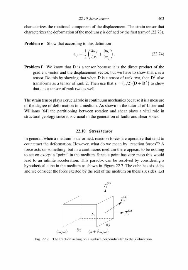
22.10 Stress tensor 403
characterizes the rotational component of the displacement. The strain tensor thatcharacterizes the deformation of the medium ε is defined by the first term of (22.73).
Problem e Show that according to this definition
εi j = 1
2
(
∂u j
∂xi+ ∂ui
∂x j
)
. (22.74)
Problem f We know that D is a tensor because it is the direct product of thegradient vector and the displacement vector, but we have to show that ε is atensor. Do this by showing that when D is a tensor of rank two, then DT alsotransforms as a tensor of rank 2. Then use that ε = (1/2)
(
D + DT)
to showthat ε is a tensor of rank two as well.
The strain tensor plays a crucial role in continuum mechanics because it is a measureof the degree of deformation in a medium. As shown in the tutorial of Lister andWilliams [64] the partitioning between rotation and shear plays a vital role instructural geology since it is crucial in the generation of faults and shear zones.
22.10 Stress tensor
In general, when a medium is deformed, reaction forces are operative that tend tocounteract the deformation. However, what do we mean by “reaction forces”? Aforce acts on something, but in a continuous medium there appears to be nothingto act on except a “point” in the medium. Since a point has zero mass this wouldlead to an infinite acceleration. This paradox can be resolved by considering ahypothetical cube in the medium as shown in Figure 22.7. The cube has six sidesand we consider the force exerted by the rest of the medium on these six sides. Let
z
(x +xy
x,y,z)(x,y,z)
Tz(x)
Ty(x)
Tx(x)
Fig. 22.7 The traction acting on a surface perpendicular to the x-direction.

404 Cartesian tensors
us focus on the side on the right that is perpendicular to the x-direction. In otherwords the normal vector to this side is orientated in the x-direction.
The force on this surface depends on the size of the surface. A meaningful way todescribe this is to use the traction, which is defined as the force per unit surface area.This traction T(x) obviously has three components which are shown in Figure 22.7;these are denoted by T (x)
x , T (x)y , and T (x)
z . The subscript refers to the component ofthe traction, the superscript refers to the fact that this is the traction on a surfaceperpendicular to the x-direction. The component T (x)
x is normal to the surface andcorresponds to a normal force, while the components T (x)
y and T (x)z are parallel to
the surface. The latter components are called the shear tractions because they causeshear motion of the medium.
When one considers the surface perpendicular to the y-direction one also findsa traction operating on that surface with components T (y)
x , T (y)y , and T (y)
z , and it isnot clear at this point whether the traction T(y) has any relation to the traction T(x)
that acts on a surface perpendicular to the x-direction. The tractions acting on thethree surfaces can be grouped in a 3 × 3 matrix:
σ ≡
⎛
⎜
⎜
⎝
......
...T(x) T(y) T(z)
......
...
⎞
⎟
⎟
⎠
=
⎛
⎜
⎝
T (x)x T (y)
x T (z)x
T (x)y T (y)
y T (z)y
T (x)z T (y)
z T (z)z
⎞
⎟
⎠. (22.75)
The quantity σ is called the stress tensor.The stress tensor has a remarkable property that is reminiscent of the property of
the gradient which was introduced in Section 5.1. The gradient is so useful becauseonce one knows the three components of the gradient, one can compute the changeof a function in any direction. The stress tensor gives the components of the tractionto surfaces that are perpendicular to the coordinates axes. One can show that thetraction on a surface that is perpendicular to an arbitrary unit vector n is givenby
T = σ · n. (22.76)
Problem a The proof of this identity is actually very simple. Consult Section 16.3of Butkov [24] or your favorite book on continuum mechanics or mathematicalphysics (that is, aside from this book) for a proof.
We have called σ the stress tensor, but we have not shown that σ is a tensor.However, one can show that when a quantity is contracted with a tensor and theresult is also a tensor, then this quantity must be a tensor as well. In (22.76) weknow that T is a tensor because it is a force (normalized with surface area) and
22.10 Stress tensor 405
we have shown in Section 22.6 that the force is a tensor of rank one. The normalvector n is also a tensor of rank one because it transforms in the same way as theposition vector. Hence we need to show from (22.76) and the fact that both T andn are tensors of rank one that σ is a tensor as well.
In components (22.76) is written as
Ti = σ i j n j , (22.77)
while the same expression in a transformed coordinate system is given by
T ′i = σ ′
i j n′j . (22.78)
Before we determine the transformation property of the stress tensor σ, we firstexpress the original vector v in terms of the transformed vector v′ using the trans-formation rule
v′i = Ci jv j . (22.45)
Problem b Multiply this expression on the left by C−1ki and sum over i to obtain
C−1ki v′
i = C−1ki Ci jv j . Use the fact that C is unitary on the left-hand side and carry
out the matrix multiplication on the right-hand side to show that Cikv′i = vk .
Finally rename i → j and k → i to obtain
vi = C jiv′j . (22.79)
It is interesting to compare this expression for the original vector v in terms of thetransformed vector v′ with (22.45) which gives the transformed vector given theoriginal vector. The only difference is the order of the subscripts in the coordinatetransform C. This is due to the fact that this matrix is unitary so that inversionamounts to interchanging the indices: C−1
i j = CTi j = C ji .
Problem c Insert (22.79) into (22.77) in order to express the unprimed vectors Tand n in terms of their transformed vectors to obtain
Cki T′
k = σ i j Cl j n′l . (22.80)
Problem d Write Cki = CTik = C−1
ik on the left-hand side and multiply by Cmi toobtain
T ′m = Cmi Cl jσ i j n
′l . (22.81)
Problem e We want to compare this expression with (22.78) in order to find σ′.However, the indices are different. As we noted earlier, the names of indices
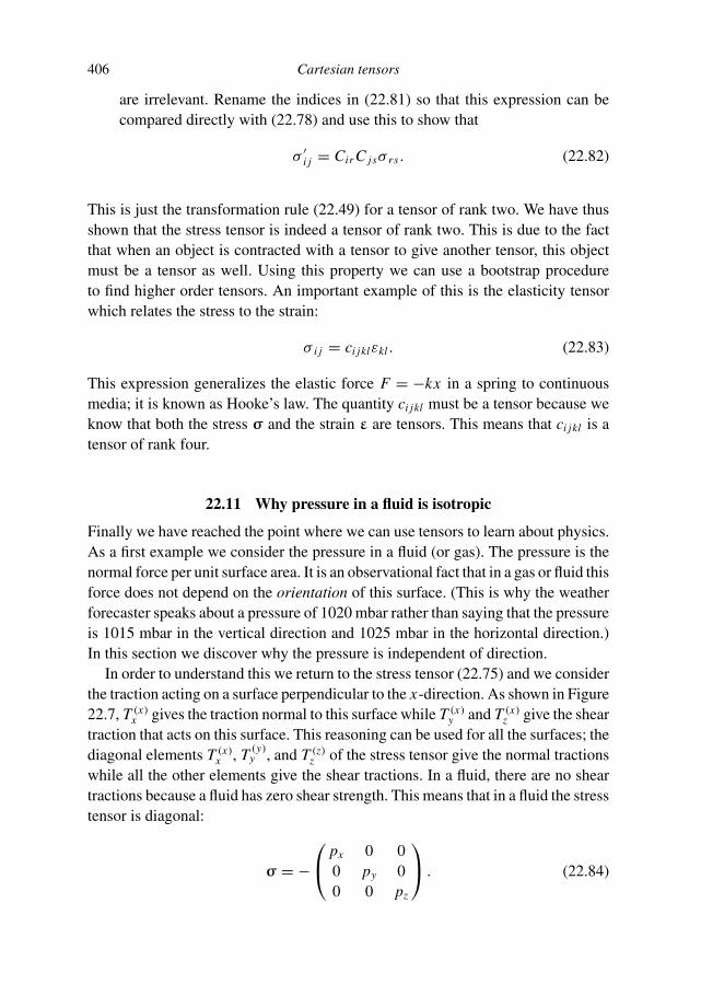
406 Cartesian tensors
are irrelevant. Rename the indices in (22.81) so that this expression can becompared directly with (22.78) and use this to show that
σ ′i j = Cir C jsσ rs . (22.82)
This is just the transformation rule (22.49) for a tensor of rank two. We have thusshown that the stress tensor is indeed a tensor of rank two. This is due to the factthat when an object is contracted with a tensor to give another tensor, this objectmust be a tensor as well. Using this property we can use a bootstrap procedureto find higher order tensors. An important example of this is the elasticity tensorwhich relates the stress to the strain:
σ i j = ci jklεkl . (22.83)
This expression generalizes the elastic force F = −kx in a spring to continuousmedia; it is known as Hooke’s law. The quantity ci jkl must be a tensor because weknow that both the stress σ and the strain ε are tensors. This means that ci jkl is atensor of rank four.
22.11 Why pressure in a fluid is isotropic
Finally we have reached the point where we can use tensors to learn about physics.As a first example we consider the pressure in a fluid (or gas). The pressure is thenormal force per unit surface area. It is an observational fact that in a gas or fluid thisforce does not depend on the orientation of this surface. (This is why the weatherforecaster speaks about a pressure of 1020 mbar rather than saying that the pressureis 1015 mbar in the vertical direction and 1025 mbar in the horizontal direction.)In this section we discover why the pressure is independent of direction.
In order to understand this we return to the stress tensor (22.75) and we considerthe traction acting on a surface perpendicular to the x-direction. As shown in Figure22.7, T (x)
x gives the traction normal to this surface while T (x)y and T (x)
z give the sheartraction that acts on this surface. This reasoning can be used for all the surfaces; thediagonal elements T (x)
x , T (y)y , and T (z)
z of the stress tensor give the normal tractionswhile all the other elements give the shear tractions. In a fluid, there are no sheartractions because a fluid has zero shear strength. This means that in a fluid the stresstensor is diagonal:
σ = −⎛
⎝
px 0 00 py 00 0 pz
⎞
⎠ . (22.84)

22.11 Why pressure in a fluid is isotropic 407
The diagonal elements pi denote the pressure in the three directions. The minussign reflects the fact that a positive pressure corresponds to a force that is directedinwards. In this section we show that the pressure is isotropic, in other words thatthe diagonal elements are identical.
Let us see what happens to the stress tensor (22.84) when we rotate the coordinatesystem through 45 degrees around the z-axis. For a rotation in two dimensionsthe rotation is given by (22.23). Setting the rotation angle ϕ to 45 degrees andextending the result to three dimensions gives the following matrix representationof this coordinate transformation:
C =⎛
⎝
1/√
2 −1/√
2 01/
√2 1/
√2 0
0 0 1
⎞
⎠ . (22.85)
Problem a Verify that this coordinate transformation is unitary.
Problem b Use the transformation property of a tensor of rank two that the stresstensor (22.84) in the rotated coordinate system is given by
σ′= −⎛
⎝
(
px + py)
/2(
px − py)
/2 0(
px − py)
/2(
px + py)
/2 00 0 pz
⎞
⎠ . (22.86)
In a fluid, the stress tensor is diagonal in any coordinate system since the sheartractions vanish in any coordinate system. This means that the off-diagonal elementsof σ′ must be equal to zero, hence px = py .
Problem c Find a suitable coordinate transform to show that px = pz .
This means that all the diagonal elements are identical; this quantity is referred toas the pressure: px = py = pz = p. In an acoustic medium such as a fluid or gasthe stress tensor is therefore given by
σ = −p I, (22.87)
so that pressure is indeed independent of direction.Note that we have done something truly remarkable; we have derived a physical
law (“the pressure is isotropic”) from the invariance of a property (“the shear stressis zero in a fluid”) under a coordinate transformation.

408 Cartesian tensors
22.12 Special relativity
One of the most spectacular applications of tensor calculus is the theory of relativitywhich describes the physics of objects and fields at very high speeds. The theoryof general relativity accounts for the fact that mass in the universe leads to a non-Cartesian structure of space-time [76]; by definition this cannot be treated with theCartesian tensors used in this chapter. The theory of special relativity describeshow different observers who both use Cartesian coordinate systems that move atgreat speeds with respect to each other describe the same physical phenomena. Aclear physical description of the theory of special relativity is given by Taylor andWheeler [105]. In this section we use the notation used by Muirhead [73] who usesa complex time variable.
Central to the theory of special relativity is the notion that space and time areintricately linked. The three position variables x , y, and z as well as time t areplaced in a four-dimensional vector, called a four-vector:
x =
⎛
⎜
⎜
⎝
xyz
ict
⎞
⎟
⎟
⎠
. (22.88)
In this expression c is the speed of light and i = √−1. The fact that the lastcomponent is complex leads to the surprising result that the length of the four-vector can be negative because
|x|2 = (x · x) = x2 + y2 + z2 − c2t2 (22.89)
and there is no reason why the last term cannot dominate the other terms.Suppose we have one observer who uses unprimed variables, and suppose that
another observer moves in the x-direction with a relative velocity v with respect tothe first observer. The two coordinate systems of the observers are then related bya Lorentz transformation [73]:
L =
⎛
⎜
⎜
⎜
⎜
⎜
⎜
⎜
⎝
1/
√
1 − v2
c20 0 i
v
c/
√
1 − v2
c2
0 1 0 0
0 0 1 0
−iv
c/
√
1 − v2
c20 0 1/
√
1 − v2
c2
⎞
⎟
⎟
⎟
⎟
⎟
⎟
⎟
⎠
. (22.90)
Problem a Show that the Lorentz transform is unitary by showing that LT L = I.
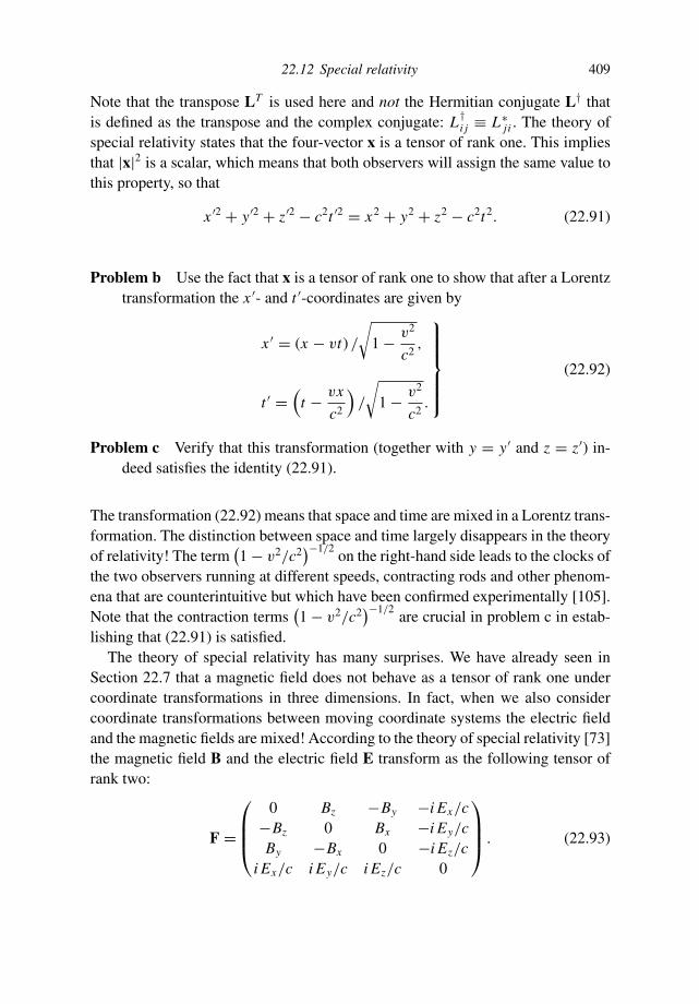
22.12 Special relativity 409
Note that the transpose LT is used here and not the Hermitian conjugate L† thatis defined as the transpose and the complex conjugate: L†
i j ≡ L∗j i . The theory of
special relativity states that the four-vector x is a tensor of rank one. This impliesthat |x|2 is a scalar, which means that both observers will assign the same value tothis property, so that
x ′2 + y′2 + z′2 − c2t ′2 = x2 + y2 + z2 − c2t2. (22.91)
Problem b Use the fact that x is a tensor of rank one to show that after a Lorentztransformation the x ′- and t ′-coordinates are given by
x ′ = (x − vt) /
√
1 − v2
c2,
t ′ =(
t − vx
c2
)
/
√
1 − v2
c2.
⎫
⎪
⎪
⎪
⎪
⎬
⎪
⎪
⎪
⎪
⎭
(22.92)
Problem c Verify that this transformation (together with y = y′ and z = z′) in-deed satisfies the identity (22.91).
The transformation (22.92) means that space and time are mixed in a Lorentz trans-formation. The distinction between space and time largely disappears in the theoryof relativity! The term
(
1 − v2/c2)−1/2
on the right-hand side leads to the clocks ofthe two observers running at different speeds, contracting rods and other phenom-ena that are counterintuitive but which have been confirmed experimentally [105].Note that the contraction terms
(
1 − v2/c2)−1/2
are crucial in problem c in estab-lishing that (22.91) is satisfied.
The theory of special relativity has many surprises. We have already seen inSection 22.7 that a magnetic field does not behave as a tensor of rank one undercoordinate transformations in three dimensions. In fact, when we also considercoordinate transformations between moving coordinate systems the electric fieldand the magnetic fields are mixed! According to the theory of special relativity [73]the magnetic field B and the electric field E transform as the following tensor ofrank two:
F =
⎛
⎜
⎜
⎝
0 Bz −By −i Ex/c−Bz 0 Bx −i Ey/cBy −Bx 0 −i Ez/c
i Ex/c i Ey/c i Ez/c 0
⎞
⎟
⎟
⎠
. (22.93)

410 Cartesian tensors
The momentum of a particle is also given by a four-vector; this momentum-energyvector [73] is given by
p =
⎛
⎜
⎜
⎝
px
py
pz
i E/c
⎞
⎟
⎟
⎠
, (22.94)
where E is the energy of the particle. This four-vector transforms as a tensor ofrank one under a Lorentz transformation [73].
Problem d Use the property that p is a tensor of rank one to show that p2 − E2/c2
is invariant, where p2 = p2x + p2
y + p2z .
Problem e In general the energy of a body is given by the energy of that bodyat rest plus a contribution due to the motion of the body. This rest energy isdenoted by E0. Show that for the particle at rest the norm of the four-vector pis given by |p|2 = −E2
0/c2 and use the result of problem d to show that
E =√
E20 + p2c2. (22.95)
This expression holds for any value of the momentum. For the moment we considera particle that moves much slower than the speed of light (p = mv mc). We shallshow that for such a particle the rest energy E0 is much larger than the energy pcthat is due to the motion.
Problem f Make a Taylor series expansion of (22.95) in the parameter pc/E0 toshow that for slow speeds
E = E0 + c2 p2
2E0− c4 p4
8E30
+ · · · . (22.96)
The first term on the right-hand side corresponds to the rest energy which we do notyet know. The second term is quadratic in the momentum. For small velocities thelaws of classical mechanics hold and the kinetic energy is given by 1
2 m0v2. Using
the classical relation p = m0v, the kinetic energy is in classical mechanics givenby p2/2m0. In classical mechanics the terms of order (cp/E0)4 are ignored. Thekinetic energy p2/2m0 in classical mechanics is therefore equal to the second termon the right-hand side of (22.96).
Problem g Derive from this statement that
E0 = m0c2. (22.97)
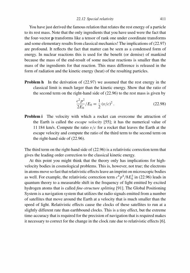
22.12 Special relativity 411
You have just derived the famous relation that relates the rest energy of a particleto its rest mass. Note that the only ingredients that you have used were the fact thatthe four-vector p transforms like a tensor of rank one under coordinate transformsand some elementary results from classical mechanics! The implications of (22.97)are profound. It reflects the fact that matter can be seen as a condensed form ofenergy. In nuclear reactions this is used for the benefit (or demise) of mankindbecause the mass of the end-result of some nuclear reactions is smaller than themass of the ingredients for that reaction. This mass difference is released in theform of radiation and the kinetic energy (heat) of the resulting particles.
Problem h In the derivation of (22.97) we assumed that the rest energy in theclassical limit is much larger than the kinetic energy. Show that the ratio ofthe second term on the right-hand side of (22.96) to the rest mass is given by
c2 p2
2E0/E0 = 1
2(v/c)2 . (22.98)
Problem i The velocity with which a rocket can overcome the attraction ofthe Earth is called the escape velocity [55]; it has the numerical value of11 184 km/s. Compute the ratio v/c for a rocket that leaves the Earth at theescape velocity and compute the ratio of the third term to the second term onthe right-hand side of (22.96).
The third term on the right-hand side of (22.96) is a relativistic correction term thatgives the leading order correction to the classical kinetic energy.
At this point you might think that the theory only has implications for high-velocity bodies in cosmological problems. This is, however, not true; the electronsin atoms move so fast that relativistic effects leave an imprint on microscopic bodiesas well. For example, the relativistic correction term c4 p4/8E3
0 in (22.96) leads inquantum theory to a measurable shift in the frequency of light emitted by excitedhydrogen atoms that is called fine-structure splitting [91]. The Global PositioningSystem is a navigation system that utilizes the radio signals emitted from a numberof satellites that move around the Earth at a velocity that is much smaller than thespeed of light. Relativistic effects cause the clocks of these satellites to run at aslightly different rate than earthbound clocks. This is a tiny effect, but the extremetime-accuracy that is required for the precision of navigation that is required makesit necessary to correct for the change in the clock rate due to relativistic effects [6].
23
Perturbation theory
From this book and most other books on mathematical physics you may have ob-tained the impression that most equations in the physical sciences can be solved.This is actually not true; most textbooks (including this book) give an unrepresen-tative state of affairs by only showing the problems that can be solved in closedform. It is an interesting paradox that as our theories of the physical world becomemore accurate, the resulting equations become more difficult to solve. In classicalmechanics the problem of two particles that interact with a central force can besolved in closed form, but the three-body problem in which three particles inter-act has no analytical solution. In quantum mechanics, the one-body problem of aparticle that moves in a potential can be solved for a limited number of situationsonly: for the free particle, the particle in a box, the harmonic oscillator, and thehydrogen atom. In this sense the one-body problem in quantum mechanics hasno general solution. This shows that as a theory becomes more accurate, the re-sulting complexity of the equations makes it often more difficult to actually findsolutions.
One way to proceed is to compute numerical solutions of the equations. Comput-ers are a powerful tool and can be extremely useful in solving physical problems.Another approach is to find approximate solutions to the equations. In Chapter 12,scale analysis was used to drop from the equations terms that appear to be irrel-evant. In this chapter, a systematic method is introduced to account for terms inthe equations that are small but that make the equations difficult to solve. The ideais that a complex problem is compared to a simpler problem that can be solvedin closed form, and to consider these small terms as a perturbation to the originalequation. The theory of this chapter then makes it possible to determine how thesolution is perturbed by the perturbation in the original equation; this techniqueis called perturbation theory. A classic reference on perturbation theory has beenwritten by Nayfeh [74]. The book by Bender and Orszag [14] gives a useful andillustrative overview of a wide variety of perturbation methods.
412
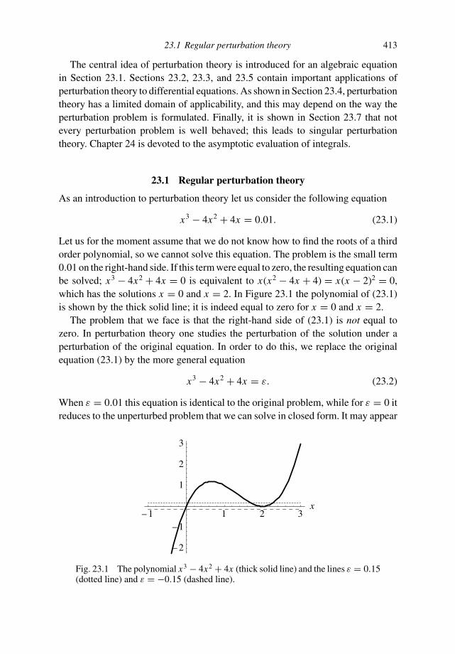
23.1 Regular perturbation theory 413
The central idea of perturbation theory is introduced for an algebraic equationin Section 23.1. Sections 23.2, 23.3, and 23.5 contain important applications ofperturbation theory to differential equations. As shown in Section 23.4, perturbationtheory has a limited domain of applicability, and this may depend on the way theperturbation problem is formulated. Finally, it is shown in Section 23.7 that notevery perturbation problem is well behaved; this leads to singular perturbationtheory. Chapter 24 is devoted to the asymptotic evaluation of integrals.
23.1 Regular perturbation theory
As an introduction to perturbation theory let us consider the following equation
x3 − 4x2 + 4x = 0.01. (23.1)
Let us for the moment assume that we do not know how to find the roots of a thirdorder polynomial, so we cannot solve this equation. The problem is the small term0.01 on the right-hand side. If this term were equal to zero, the resulting equation canbe solved; x3 − 4x2 + 4x = 0 is equivalent to x(x2 − 4x + 4) = x(x − 2)2 = 0,which has the solutions x = 0 and x = 2. In Figure 23.1 the polynomial of (23.1)is shown by the thick solid line; it is indeed equal to zero for x = 0 and x = 2.
The problem that we face is that the right-hand side of (23.1) is not equal tozero. In perturbation theory one studies the perturbation of the solution under aperturbation of the original equation. In order to do this, we replace the originalequation (23.1) by the more general equation
x3 − 4x2 + 4x = ε. (23.2)
When ε = 0.01 this equation is identical to the original problem, while for ε = 0 itreduces to the unperturbed problem that we can solve in closed form. It may appear
– 1 1 2 3x
– 2
– 1
1
2
3
Fig. 23.1 The polynomial x3 − 4x2 + 4x (thick solid line) and the lines ε = 0.15(dotted line) and ε = −0.15 (dashed line).

414 Perturbation theory
that we have made the problem more complex because we still need to solve thesame equation as our original equation, but it now contains a new variable ε aswell! However, this is also the strength of this approach.
The solution of (23.2) is a function of ε so that
x = x(ε) . (23.3)
In Section 3.1 the Taylor series was used to approximate a function f (x) by a powerseries in the variable x :
f (x) = f (0) + xd f
dx(x = 0) + x2
2!
d2 f
dx2(x = 0) + · · · . (3.11)
When the solution x of (23.2) depends in a regular way on ε, this solution can alsobe written as a similar power series by making the substitutions x → ε and f → xin (3.11):
x(ε) = x(0) + εdx
dε(ε = 0) + ε2
2!
d2x
dε2(ε = 0) + · · · . (23.4)
This expression is not very useful because we need the derivative dx/dε and higherderivatives dnx/dεn as well; in order to compute these derivatives we need to findthe solution x(ε) first, but this is just what we are trying to do. There is, however,another way to determine the series (23.4). Let us write the solution x(ε) as a powerseries in ε
x(ε) = x0 + εx1 + ε2x2 + · · · . (23.5)
The coefficients xn are not known at this point, but once we know them the solution xcan be found by inserting the numerical value ε = 0.01. In practice one truncates theseries (23.5); it is this truncation that makes perturbation theory an approximation.
When the series (23.5) is inserted into (23.2) one needs to compute x2 and x3
when x is given by (23.5). Let us first consider the x2-term. The square of a sum ofterms is given by
(a + b + c + · · ·)2 = a2 + b2 + c2 + · · ·+ 2ab + 2ac + 2bc + · · · . (23.6)
Let us apply this to the series (23.5) and retain only the terms up to order ε2, thisgives
(
x0 + εx1 + ε2x2 + · · ·)2 = x20 + ε2x2
1 + ε4x22 + · · ·
+ 2εx0x2 + 2ε2x0x2 + 2ε3x1x2 + · · · . (23.7)
If we are only are interested in retaining the terms up to order ε2, the terms ε4x22
and 2ε3x1x2 in this expression can be ignored. Collecting terms of equal powers of

23.1 Regular perturbation theory 415
ε then gives(
x0 + εx1 + ε2x2 + · · ·)2 = x20 + 2εx0x1 + ε2
(
x21 + 2x0x2
) + O(ε3). (23.8)
A similar expansion in powers of ε can be used for the term x3. This expansion isbased on the identity
(a + b + c + · · ·)3 = a3 + b3 + c3 + · · ·+ 3a2b + 3ab2 + 3a2c + 3ac2 + 3b2c + 3bc2 + · · · .
(23.9)
Problem a Apply this identity to the series (23.5), collect together all the termswith equal powers of ε and show that up to order ε2 the result is given by
(
x0 + εx1 + ε2x2 + · · ·)3 = x30 + 3εx2
0 x1 + 3ε2(
x0x21 + x2
0 x2) + O(ε3). (23.10)
Problem b At this point we can express all the terms in (23.2) in a power seriesof ε. Insert (23.5), (23.8), and (23.10) into the original equation (23.2) andcollect together terms of equal powers of ε to derive that
x30 − 4x2
0 + 4x0
+ ε(
3x20 x1 − 8x0x1 + 4x1 − 1
)
+ ε2 (
3x0x21 + x2
0 x2 − 4x21 − 8x0x2 + 4x2
) + · · · = 0 . (23.11)
In this and subsequent expressions the dots denote terms of order O(ε3). Theterm −1 in the term that multiplies ε comes from the right-hand side of (23.2).
At this point we use that ε does not have a fixed value, but that it can take any valuewithin certain bounds. This means that expression (23.11) must be satisfied for arange of values of ε. This can only be the case when the coefficients that multiplythe different powers εn are equal to zero. This means that (23.11) is equivalent tothe following system of equations which consists of the terms that multiply theterms ε0, ε1 and ε2 respectively:
O(1)-terms: x30 − 4x2
0 + 4x0 = 0,
O(ε)-terms: 3x20 x1 − 8x0x1 + 4x1 − 1 = 0,
O(ε2)-terms: 3x0x21 + x2
0 x2 − 4x21 − 8x0x2 + 4x2 = 0 .
⎫
⎬
⎭
(23.12)
You may wonder whether we have not made the problem more complex. We startedwith a single equation for a single variable x , and now we have a system of coupledequations for many variables. However, we could not solve (23.2) for the singlevariable x , while it is not difficult to solve (23.12).

416 Perturbation theory
Problem c Show that (23.12) can be rewritten in the following form:
x30 − 4x2
0 + 4x0 = 0,(
3x20 − 8x0 + 4
)
x1 = 1,(
x20 − 8x0 + 4
)
x2 = (4 − 3x0) x21 .
⎫
⎬
⎭
(23.13)
The first equation is simply the unperturbed problem, this has the solutions x0 = 0and x0 = 2. For reasons that will become clear in Section 23.7 we focus here on thesolution x0 = 0 only. Given x0, the parameter x1 follows from the second equationbecause this is a linear equation in x1. The last equation is a linear equation in theunknown x2 which can easily be solved once x0 and x1 are known.
Problem d Solve (23.13) in this way to show that the solution near x = 0 is givenby
x0 = 0, x1 = 1
4, x2 = 1
16. (23.14)
Now we are close to the final solution of our problem. The coefficients of theprevious expression can be inserted into the perturbation series (23.5) so that thesolution as a function of ε is given by
x = 0 + 1
4ε + 1
16ε2 + O(ε3) . (23.15)
At this point we can revert to the original equation (23.1) by inserting the numericalvalue ε = 0.01, which gives:
x = 1
4× 10⁻² + 1
16× 10−4 + O(10−6) = 0.002506 . (23.16)
It should be noted that this is an approximate solution because the terms of orderε3 and higher have been ignored. This is indicated by the term O(10−6) in (23.16).Assuming that the error made by truncating the perturbation series is of the sameorder as the first term that is truncated, the error in the solution (23.16) is of theorder 10−6. For this reason the number on the right-hand side of (23.16) is given tosix decimals; the last decimal is of the same order as the truncation error.
If this result is not sufficiently accurate for the application that one has in mind,then one can easily extend the analysis to higher powers εn in order to reduce thetruncation error of the truncated perturbation series. Although the algebra resultingfrom doing this can be tedious, there is no reason why this analysis cannot beextended to higher orders.
A truly formal analysis of perturbation problems can be difficult. For example,the perturbation series (23.5) converges only for sufficiently small values of ε. It is
23.2 Born approximation 417
often not clear whether the employed value of ε (in this case ε = 0.01) is sufficientlysmall to ensure convergence. Even when a perturbation series does not convergefor a given value of ε, one can often obtain a useful approximation to the solutionby truncating the perturbation series at a suitably chosen order [14]. In this caseone speaks of an asymptotic series.
When one has obtained an approximate solution of a perturbation problem, onecan sometimes substitute it back into the original equation to verify whether thissolution indeed satisfies the equation with an acceptable accuracy. For example,inserting the numerical value x = 0.002 506 in (23.1) gives
x3 − 4x2 + 4x = 0.009 998 9 = 0.01 − 0.000 001 1 . (23.17)
This means that the approximate solution satisfies (23.1) with a relative error thatis given by 0.000 001 1/0.01 = 10−4. This is a very accurate result given the factthat only three terms were retained in the perturbation analysis of this section.
23.2 Born approximation
In many scattering problems one wants to account for the scattering of waves bythe heterogeneities in the medium. Usually these problems are so complex that theycannot be solved in closed form. Suppose one has a background medium in whichscatterers are embedded. When the background medium is sufficiently simple, onecan solve the wave propagation problem for this background medium. For example,in Section 19.3 we computed the Green’s function for the Helmholtz equation in ahomogeneous medium.
In this section we consider the Helmholtz equation with a variable velocity c(r)as an example of the application of perturbation theory to scattering problems. Thismeans we consider the wave field p(r, ω) in the frequency domain that satisfies thefollowing equation:
∇2 p(r, ω) + ω2
c2(r)p(r, ω) = S(r, ω) . (23.18)
In this expression S(r, ω) denotes the source that generates the wave field. In orderto facilitate a systematic perturbation analysis we decompose 1/c2(r) into a term1/c2
0 that accounts for a homogeneous reference model and a perturbation:
1
c2(r)= 1
c20
[1 + εn(r)] . (23.19)
In this expression ε is a small parameter which measures the strength of the het-erogeneity. The function n(r) gives the spatial distribution of the heterogeneity.Combining the previous expressions it follows that the wave field satisfies the

418 Perturbation theory
following expression:
∇2 p(r, ω) + ω2
c20
[1 + εn(r)] p(r, ω) = S(r, ω). (23.20)
The solution p(r, ω) of this expression is a function of the scattering strength ε; forsufficiently small values of ε it can be written as a power series in ε:
p = p0 + εp1 + ε2 p2 + · · · . (23.21)
Problem a Insert the perturbation series (23.21) into (23.20), collect together theterms that multiply equal powers of ε and show that the terms that multiplythe different powers of ε give the following equations:
O(1) : ∇2 p0(r, ω) + ω2
c20
p0(r, ω) = S(r, ω),
O(ε) : ∇2 p1(r, ω) + ω2
c20
p1(r, ω) = −ω2
c20
n(r)p0(r, ω),
O(ε2) : ∇2 p2(r, ω) + ω2
c20
p2(r, ω) = −ω2
c20
n(r)p1(r, ω),
...
⎫
⎪
⎪
⎪
⎪
⎪
⎪
⎪
⎪
⎪
⎪
⎪
⎬
⎪
⎪
⎪
⎪
⎪
⎪
⎪
⎪
⎪
⎪
⎪
⎭
(23.22)
The first expression gives the Helmholtz equation for a homogeneous medium. Thesource of the unperturbed wave p0 is given by S(r, ω) which is also the sourceof the perturbed problem. The source of the first order perturbation p1 is givenby the right-hand side of the second equation, hence the source of p1 is givenby − (
ω2/c20
)
n(r)p0(r, ω). This means that the source of p1 is proportional tothe inhomogeneity n(r) of the medium. Physically this corresponds to the factthat the heterogeneity is the source of the scattered waves. The source of p1 isalso proportional to the unperturbed wave field p0. The reason for this is that thegeneration of the scattered waves depends on the local perturbation of the mediumas well as on the strength of the wave field at the location of the scatterers.
Each of the equations in (23.22) is of the form ∇2 p(r, ω) + ω2/c20 p(r, ω) =
F(r, ω). According to the theory of Section 18.4 the solution to this expression isgiven by
p(r, ω) =∫
G0(r, r′; ω)F(r′, ω) dV ′, (23.23)
where the unperturbed Green’s function G0(r, r′; ω) is the response in a homoge-neous medium at location r due to a point source at location r′:
∇2G0(r, r′; ω) + ω2
c20
G0(r, r′; ω) = δ(r − r′). (23.24)
23.2 Born approximation 419
The specific form of the unperturbed Green’s function in one, two, and three di-mensions is given in (19.43). From this point on it is not shown explicitly that thesolution and the Green’s function depend on the angular frequency ω, but it shouldbe kept in mind that all the results in this section depend on frequency.
Problem c Use these results to show that the solution of (23.22) is given by
p0(r) = ∫
G0(r, r′)S(r′) dV ′,
p1(r) = −ω2
c20
∫
G0(r, r′)n(r′)p0(r′) dV ′,
p2(r) = −ω2
c20
∫
G0(r, r′)n(r′)p1(r′) dV ′,
...
⎫
⎪
⎪
⎪
⎪
⎪
⎪
⎪
⎪
⎪
⎬
⎪
⎪
⎪
⎪
⎪
⎪
⎪
⎪
⎪
⎭
(23.25)
Problem d Insert the expression for the unperturbed wave p0 into the secondequation (23.25) to show that the first order perturbation is given by
p1(r) = −ω2
c20
∫∫
G0(r, r1)n(r1)G0(r1, r0)S(r0) dV1dV0. (23.26)
Note that the integration variable r′ has been relabeled as r0 and r1 respectively.
Problem e Insert this result in the last line of (23.25) to derive that the secondorder perturbation is given by
p2(r) = ω4
c40
×∫∫∫
G0(r, r2)n(r2)G0(r2, r1)n(r1)G0(r1, r0)S(r0) dV2dV1dV0.
(23.27)
Inserting this result and (23.25) in the perturbation series (23.21) finally gives thefollowing perturbation series for the scattered waves:
p(r, ω) =∫
G0(r, r0)S(r0) dV0
− ω2
c20
∫∫
G0(r, r1)n(r1)G0(r1, r0)S(r0) dV1dV0
+ ω4
c40
∫∫∫
G0(r,r2)n(r2)G0(r2,r1)n(r1)G0(r1,r0)S(r0) dV2dV1dV0
+ · · · . (23.28)

420 Perturbation theory
G S G S G nG S G nG nG S
singlescattered
wave
doublescattered
wave
unperturbedwave
totalwave
= + + + . . .
0 00 000
Fig. 23.2 Decomposition of the total wave field (thick solid line) in the unper-turbed wave, the single scattered wave, the double scattered wave, and higherorder scattering events. The total Green’s function G is shown by a thick line, theunperturbed Green’s function G0 by thin lines, and each scattering event by theheterogeneity n is indicated by a solid dot.
This expansion is shown graphically in Figure 23.2. Reading each of the lines inexpression (23.28) from right to left one can follow the “life-history” of the wavesthat are scattered in the medium. The top line of the right-hand side gives the unper-turbed wave. This wave is excited by the source at location r0; this is described bythe source term S(r0). The wave then propagates through the unperturbed mediumto the point r; this is accounted for by the term G0(r, r0). Graphically this is shownby the first diagram after the equality sign in Figure 23.2. In this figure the thinarrows denote the unperturbed Green’s function G0. The second line in (23.28)physically describes a wave that is generated at the source S(r0); this wave thenpropagates through the unperturbed medium with the Green’s function G0(r1, r0)to a scatterer at location r1. The wave is then scattered; this is accounted for by theterms − (
ω2/c20
)
n(r1). In Figure 23.2 this scattering interaction is indicated by asolid dot. The wave then travels through the unperturbed medium to the point r;this is accounted for by the term G0(r, r1).
Problem f Describe in a similar way the “life-history” of the double scatteredwave that is given by the last line of (23.28) and convince yourself that thiscorresponds to the right-most diagram in Figure 23.2.
The analysis in this section can be continued to any order. The resulting series iscalled the Neumann series. It gives a decomposition of the total wave field into singlescattered waves, double scattered waves, triple scattered waves, etc. In practice it isoften difficult to compute the waves that are scattered more than once. In the Bornapproximation one simply truncates the perturbation series after the second term.Using the notation of (23.25) this means that in the Born approximation the wavefield is given by
pB(r) = p0(r) − ω2
c20
∫
G0(r, r′)n(r′)p0(r′) dV ′. (23.29)

23.3 Linear travel time tomography 421
This expression is extremely useful for a large variety of applications. For suffi-ciently weak perturbations εn(r) it allows the analytical computation of the (single)scattered waves. In the Born approximation the scattered waves are given by the lastterm in (23.29). This last term gives a linear(ized) relation between the scatteredwaves and the perturbation of the medium. In many applications one measuresthe scattered waves and one wants to retrieve the perturbation of the medium. TheBorn approximation provides a linear relation between the scattered waves and theperturbation of the medium. Methods from linear algebra can then be used to inferthe perturbation n(r) of the medium from measurements of the scattered waves.The Born approximation provides the basis for most of the techniques used inreflection seismology for the detection of hydrocarbons in the Earth, see for ex-ample references [28] and [123]. The Born approximation also forms the basis ofthe imaging techniques used with radar [52] and a variety of other applications. Infact, it has been argued that imaging with multiple-scattered waves is not feasible inpractice [28]; a discussion of this controversial issue can be found in reference [92].
In this section the Born approximation for the Helmholtz equation was derived.However, this derivation can readily be generalized to other scattering problems.The only required ingredient is that, when one divides the medium into an unper-turbed medium and a perturbation, one can compute the Green’s function for theunperturbed medium. The Born approximation is used in quantum mechanics [69],electromagnetic wave scattering [53], scattering of elastic body waves [122], andelastic surface waves [97].
There is a famous application of the Born approximation. According to (23.29)the scattered waves are multiplied by ω2 compared to the unperturbed waves. This isalso the case for the scattering of electromagnetic waves [53]. This term ω2 explainswhy the sky is blue. The scattered waves are proportional to ω2 compared to theunperturbed waves. This means that light with a high frequency is scattered morestrongly than light with a lower frequency. In other words, blue light is scatteredmore strongly than red light. The blue light that comes from the Sun is scatteredmore effectively out of the light beam from the Sun to an observer than the red light.When this blue light is scattered again by small particles in the atmosphere it travelsto an observer as blue light that comes from the sky from a different location thanthe Sun. We perceive this as “the blue sky.” This argument should, however, be usedwith caution because the Green’s function in (23.29) also depends on frequency.
23.3 Linear travel time tomography
An important tool for determining the interior structure of the Earth and otherbodies is travel time tomography. In this technique one measures the travel time ofwaves between a large number of sources and receivers. When the coverage with
422 Perturbation theory
rays is sufficiently dense, one can determine the velocity of seismic waves in theEarth from the recorded travel times. Detailed descriptions of seismic tomographycan be found in references [51] and [75]. The travel time along a ray is given bythe integral
τ =∫
1
c(r)ds. (23.30)
Since the integral is proportional to 1/c(r), it is convenient to use the slownessu(r) = 1/c(r) rather than the velocity. Using this quantity the travel time is givenby
τ =∫
r[u]u(r) ds. (23.31)
The last expression suggests a linear relation between the measured travel timeτ and the unknown slowness u(r). Such a linear relation is ideal for solving theinverse problem of the determination of the slowness because one can resort totechniques from linear algebra. However, integral (23.31) is taken over the ray thatjoins the source and the receiver. The rays are curves of stationary travel time andthemselves depend on the slowness. This dependence effectively makes the relationbetween the slowness and the travel time nonlinear. In this section we perturb boththe slowness and the travel time to derive a linearized relation between the traveltime perturbation and the slowness perturbation. The travel time along rays followsfrom geometric ray theory as shown in Section 12.4. It is shown in that section thatthe travel time τ (r) from a given source to location r is given by the eikonal equation(12.25) which can be written as
|∇τ (r)|2 = u2(r). (23.32)
Let us assume that we have a reasonable guess u0(r) for the slowness, and thatwe seek a small perturbation of the slowness; this perturbation is denoted as εu1(r).The slowness can then be written as
u(r) = u0(r) + εu1(r). (23.33)
Again, the parameter ε only serves to systematically set up the perturbation treat-ment. When the slowness is perturbed, the travel time changes as well and it canbe expanded in a perturbation series of the parameter ε:
τ = τ 0 + ετ 1 + ε2τ 2 + · · · . (23.34)
In this section we seek the relation between the first order travel time perturbationτ 1 and the slowness perturbation u1.
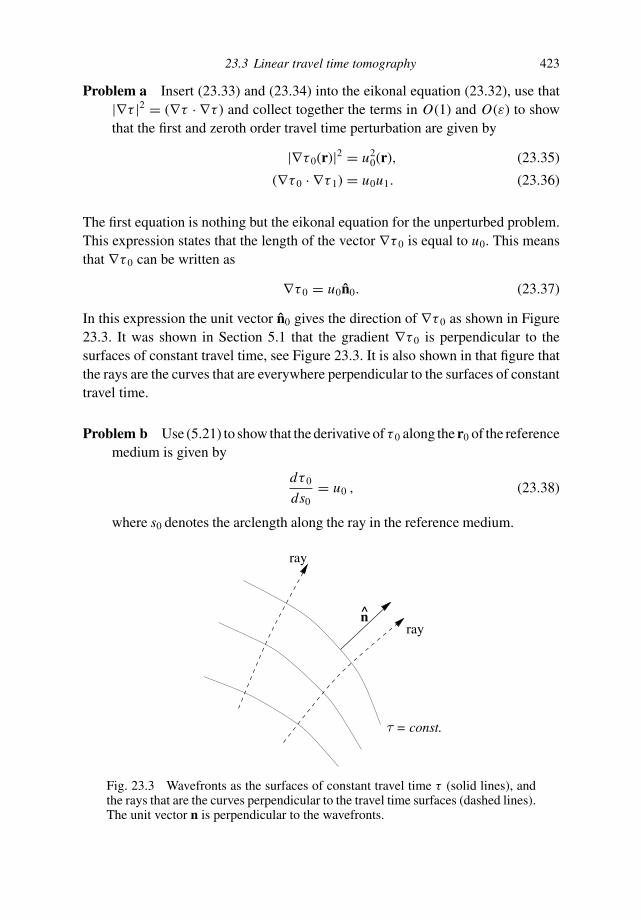
23.3 Linear travel time tomography 423
Problem a Insert (23.33) and (23.34) into the eikonal equation (23.32), use that|∇τ |2 = (∇τ · ∇τ ) and collect together the terms in O(1) and O(ε) to showthat the first and zeroth order travel time perturbation are given by
|∇τ 0(r)|2 = u20(r), (23.35)
(∇τ 0 · ∇τ 1) = u0u1. (23.36)
The first equation is nothing but the eikonal equation for the unperturbed problem.This expression states that the length of the vector ∇τ 0 is equal to u0. This meansthat ∇τ 0 can be written as
∇τ 0 = u0n0. (23.37)
In this expression the unit vector n0 gives the direction of ∇τ 0 as shown in Figure23.3. It was shown in Section 5.1 that the gradient ∇τ 0 is perpendicular to thesurfaces of constant travel time, see Figure 23.3. It is also shown in that figure thatthe rays are the curves that are everywhere perpendicular to the surfaces of constanttravel time.
Problem b Use (5.21) to show that the derivative of τ 0 along the r0 of the referencemedium is given by
dτ 0
ds0= u0 , (23.38)
where s0 denotes the arclength along the ray in the reference medium.
= const.
n
ray
ray
Fig. 23.3 Wavefronts as the surfaces of constant travel time τ (solid lines), andthe rays that are the curves perpendicular to the travel time surfaces (dashed lines).The unit vector n is perpendicular to the wavefronts.

424 Perturbation theory
This last expression can be integrated to give
τ 0 =∫
r0[u0]u0(r) ds0. (23.39)
This expression is identical to (23.31) with the exception that all quantities are forthe reference medium u0 and its associated rays r0[u0].
Problem c In order to derive the first order travel time perturbation, insert (23.37)into (23.36) to derive that
(n0 · ∇τ 1) = u1. (23.40)
Note that the unit vector n0 is directed along the rays in the reference mediumu0 and that it is therefore independent of the slowness perturbation u1.
Problem d Integrate the last expression to give
τ 1 =∫
r0[u0]u1(r) ds0. (23.41)
In this expression the integration is along the rays r0[u0] in the reference medium.Since these rays are assumed to be known, (23.41) constitutes a linearized relationbetween the travel time perturbation τ 1 and the slowness perturbation u1. Tech-niques from linear algebra can then be used to determine the unknown slownessperturbation from the measured travel time perturbations τ 1. In many textbooks (e.g.reference [75]) this result is derived from Fermat’s theorem. However, the treatmentin this section (which was proposed by Aldridge [4]) is conceptually much simpler.In fact, the treatment in this section can easily be extended to compute the traveltime perturbation to any order [99].
23.4 Limits on perturbation theory
Perturbation theory is a powerful tool; in principle it provides a systematic way toderive the perturbation to any desired order. In this section we will discover that fora given order of truncation of the perturbation series the accuracy of the obtainedresult may depend strongly on the value of certain parameters of the problem thatone is considering. This is illustrated with a simple problem which we can alsosolve analytically. We consider the differential equation
x + ω20 (1 + ε) x = 0, (23.42)

23.4 Limits on perturbation theory 425
with the initial conditions
x(0) = 1, x(0) = 0. (23.43)
This equation describes a harmonic oscillator in which the frequency is perturbed.
Problem a Show that the exact solution of this problem is given by
x(t) = cos(
ω0
√1 + ε t
)
. (23.44)
Problem b The solution x(t) is a function of the perturbation parameter ε, it cantherefore be written as a perturbation series in this parameter:
x(t) = x0(t) + εx1(t) + ε2x2(t) + · · · . (23.45)
Insert this series into (23.42) and collect together the terms of equal powersin ε to show that the terms xn(t) satisfy the following equations:
x0 + ω20x0 = 0,
x1 + ω20x1 = −ω2
0x0,
x2 + ω20x2 = −ω2
0x1,
...
⎫
⎪
⎪
⎪
⎪
⎬
⎪
⎪
⎪
⎪
⎭
(23.46)
Problem c In order to solve these equations one must also consider the initialconditions of xn(t). Obtain these condition by inserting the perturbation series(23.45) into the initial conditions (23.43) and derive that
x0(0) = 1, x0(0) = 0 ,
xn(0) = 0, xn(0) = 0 for n ≥ 1.
(23.47)
Problem d Solve the differential equation for x0 for the boundary condition of(23.47) and show that the solution is given by
x0(t) = cos (ω0t) . (23.48)
Note that this expression is identical to the exact solution (23.44) when oneswitches off the perturbation by setting ε = 0. Inserting this solution into the secondline of (23.46) one finds that the first order perturbation satisfies the followingdifferential equation
x1 + ω20x1 = −ω2
0 cos (ω0t) . (23.49)
This equation describes a harmonic oscillator with eigenfrequency ω0 which isdriven by a force on the right-hand side. This driving force also oscillates with
426 Perturbation theory
frequency ω0. This means that the oscillator x1 is driven at its resonance frequency,which in general leads to a motion that grows with time.
Problem e In order to solve (23.49) write the perturbation x1(t) as
x1(t) = f (t) cos (ω0t) + g(t) sin (ω0t) . (23.50)
Insert this expression into (23.49) and collect together the terms that multiplycos (ω0t) and sin (ω0t) to show that the unknown functions f (t) and g(t) obeythe following differential equations:
f + 2ω0g = −ω20,
g − 2ω0 f = 0.
(23.51)
Problem f Show that these equations are satisfied by the following solution:
f = 0, g = − ω0
2, (23.52)
and integrate these equations to derive a particular solution that is given by
f = A, g(t) = − 1
2ω0t + B, (23.53)
with A and B integration constants.
These expressions for f and g lead to the general solution
x1(t) = − 1
2ω0t sin (ω0t) + A cos (ω0t) + B sin (ω0t) . (23.54)
It follows from (23.47) that the initial conditions for x1(t) are given by x1(0) = 0,x(0) = 0.
Problem g Derive from these initial conditions that the integration constants aregiven by A = B = 0, so that the solution is given by
x1(t) = − 1
2ω0t sin (ω0t) . (23.55)
It was noted earlier that (23.49) describes an oscillator that is driven at its reso-nance frequency. Solution (23.55) grows linearly with time. This growth with timeis called the secular growth. It is an artifact of the perturbation technique employedbecause the original problem (23.42) does not contain a resonant driving force at all.Inserting the first order perturbation (23.55) and the unperturbed solution (23.48)into the perturbation series (23.45) finally gives
x(t) = cos (ω0t) − ε
2ω0t sin (ω0t) + O(ε2). (23.56)

23.5 WKB approximation 427
Let us first verify that this expression is indeed the first order expansion of theexact solution (23.44). Using the series (3.12), (3.13), and (3.16), the exact solution(23.44) is to first order in ε given by
x(t) = cos(
ω0
√1 + ε t
)
= cos
ω0
[
1 + ε
2+ O(ε2)
]
t
= cos (ω0t) cos(ε
2ω0t
)
− sin (ω0t) sin(ε
2ω0t
)
+ O(ε2)
= cos (ω0t) − ε
2ω0t sin (ω0t) + O(ε2) (23.57)
This result is indeed identical to the first order expansion (23.56) that was obtainedfrom perturbation theory. The fact that this result is correct, however, does notimply that this result is also useful. Perturbation theory is based on the premisethat the truncated perturbation series gives a good approximation to the true solu-tion. The truncation of this series only makes sense when the subsequent terms inthe perturbation expansion rapidly become smaller. However, the first order term(εω0t/2) sin (ω0t) in (23.46) is as large as the zeroth order term cos (ω0t) whenεω0t/2 ∼ 1. This means that the first order perturbation series (23.56) ceases to bea good approximation to the true solution when
t ∼ 1
εω0. (23.58)
The upshot of this example is that even though a truncated perturbation series maybe correct, it may only be useful for a restricted range of parameters. In this examplethe first order perturbation series is a good approximation only when t 1/εω0.For the problem in this section it would be more appropriate to make a perturbationseries of the phase and the amplitude of the oscillator. Systematic techniques such asmultiple-scale analysis [14] have been developed for this purpose. In the followingsection we carry out the transformation p = eS to derive the perturbations of theamplitude and phase of a wave that propagates through an inhomogeneous medium.
23.5 WKB approximation
In this section we analyze the propagation of a wave through a one-dimensionalacoustic medium. In the frequency domain the pressure satisfies the followingdifferential equation:
ρd
dx
(
1
ρ
dp
dx
)
+ ω2
c2p = 0. (23.59)
In this expression both the density ρ and the velocity c vary with the position x .This equation can only be solved in closed form for a special form of the functions

428 Perturbation theory
ρ(x) and c(x). It should be noted that the treatment in this section is also applicableto the Schrodinger equation
d2ψ
dx2+ 2m
h2 [E − V (x)] ψ = 0, (23.60)
by making the substitutions
ρ(x) → 1, p → ψ, 1/c(x) →√
2m (E − V (x))/hω. (23.61)
At this point there is as yet no small perturbation parameter. We restrict ourattention to media in which the length scale of each variation in ρ and c is muchlarger than the wavelength λ of the wave. Physically this type of medium does notcontain strong inhomogeneities on the scale of a wavelength, so that the waves arenot reflected strongly by the heterogeneity. Let the length scale of the heterogeneitybe denoted by L . When this length scale is much larger than the wavelength λ =2πω/c, the following parameter is small:
ε = c
ωL 1. (23.62)
As noted in the previous section, when the perturbation affects mostly the phaseof a wave, it is advantageous to perturb the phase (and amplitude) of the wave ratherthan the solution p itself. This can be achieved by making the transformation
p = eS. (23.63)
When S is complex this transformation is without any loss of generality.
Problem a Insert this relation into (23.59) and derive that S(x) satisfies the fol-lowing differential equation:
d2S
dx2− 1
ρ
dρ
dx
d S
dx+
(
d S
dx
)2
+ ω2
c2= 0. (23.64)
At this point we have made the problem more complex because this equation isnonlinear in the unknown function S(x) whereas the original equation (23.59) islinear in the pressure p(x). However, we have not yet applied the perturbationtechnique. Before we do this, let us first reflect on the transformation (23.63).If the medium were homogeneous, the solution would be given by p = Aeikx ,with the wavenumber given by k = ω/c. This special solution corresponds to S =ln (A) + ikx , so that d S/dx = ik = iω/c. For an inhomogeneous medium one mayexpect the derivative of the phase to be close to this value, therefore we make the

23.5 WKB approximation 429
following substitution:
d S
dx= iω
c(x)F(x). (23.65)
Problem b Show that this transformation transforms (23.64) into the followingdifferential equation for F :
d F
dx− 1
ρc
d (ρc)
dxF + iω
cF2 = iω
c. (23.66)
Now we use perturbation analysis by using that the parameter ε defined in (23.62)is much smaller than unity. This can be achieved by transforming the distance x toa dimensionless distance ξ defined by
ξ ≡ x/L , (23.67)
where L is the characteristic length scale of the velocity and density variations.
Problem c Under this transformation the derivative d/dx changes to d/dx =d/d(ξ L) = (1/L) d/dξ . Use this to show that F(ξ ) satisfies the followingdifferential equation:
c
ωL
d F
dξ− c
ωL
1
ρc
d (ρc)
dξF + i F2 = i. (23.68)
This equation contains the small dimensionless parameter c/ωL defined in (23.62),so that this equation is equivalent to
εd F
dξ− ε
1
ρc
d (ρc)
dξF + i F2 = i. (23.69)
Now we have an equation that looks similar to those in the perturbation problemswe have seen in this chapter. We solve this equation by inserting the followingperturbation series for F(ξ ):
F(ξ ) = F0(ξ ) + εF1(ξ ) + · · · . (23.70)
Problem d Insert this perturbation series into the differential equation(23.69) to derive that F0(ξ ) and F1(ξ ) satisfy the following equations:
F20 = 1,
2i F0 F1 = −d F0
dξ+ 1
ρc
d (ρc)
dξF0.
⎫
⎪
⎬
⎪
⎭
(23.71)
430 Perturbation theory
The first of these equations has the solutions F0 = ±1. According to (23.65) thiscorresponds to the phase derivative d S/dx = ±iω/c. The plus sign denotes a right-going wave, and the minus sign a left-going wave. We focus here on a right-goingwave so that F0 = +1.
Problem e Insert this solution into the second line of (23.71) and show that F1(x ′)is given by
F1(ξ ) = − i
2
1
ρc
d (ρc)
dξ. (23.72)
This means that the first-order perturbation series for F(ξ ) is given by
F(ξ ) = 1 − iε
2
1
ρc
d (ρc)
dξ+ O(ε2). (23.73)
Problem f Now that we have obtained this solution as a function of the trans-formed distance ξ , transform back to the original distance x by using (23.67).Use (23.62) to show that the solution (23.73) is equivalent to
F(x) = 1 − i
2
1
ρω
d (ρc)
dx+ · · · . (23.74)
Problem g Use (23.65) to convert this into an equation for d S/dx . Integrate thisequation to show that the solution S(x) is given by
S(x) = i∫ x
−∞
ω
c(x ′)dx ′ + 1
2ln [ρ(x)c(x)] + B. (23.75)
Problem h Use the transformation (23.63) to show that this solution correspondsto the following pressure field
p(x) = A√
ρ(x)c(x) exp
(
i∫ x
−∞
ω
c(x ′)dx ′
)
, (23.76)
with the new constant defined by A = eB .
This solution states that the wave propagates to the right with an amplitude thatis proportional to
√ρ(x)c(x). The local wavenumber k(x) of the wave is given by
the derivative of the phase of the wave [119]; it is therefore given by
k(x) = d
dx
∫ x
−∞
ω
c(x ′)dx ′ = ω
c(x). (23.77)
This means that the local wavenumber at a location x is given by the wavenumberω/c(x) that the medium would have if it were homogeneous with the properties of
23.6 Need for consistency 431
the medium at that location x . The solution (23.76) is known as the WKB solution(named after Wentzel, Kramers, and Brillouin). Seismologists prefer to call thissolution the WKBJ approximation because of the contribution of Lord Jeffreys [54].
In most textbooks (e.g. reference [69]) this solution is derived for the Schrodingerequation rather than the acoustic wave equation; with the transformation (23.61)the derivations are equivalent.
Problem i Use the correspondence (23.61) to show that in quantum mechanicsthe WKB solution is given by
ψ(x) = A
[E − V (x)]1/4 exp
i∫ x
−∞
√2m [E − V (x ′)]
hdx ′
. (23.78)
Problem j Show that this approximation is infinite at the turning points of themotion. These are the points where the total energy of the particle is equal tothe potential energy. This means that the WKB solution breaks down at theturning points.
A clear account of the WKB approximation with a large number of applications isgiven by Bender and Orszag [14].
23.6 Need for consistency
In perturbation theory one derives an approximate solution to a problem. In manyapplications this approximation is then used in subsequent calculations. In doingso, one must keep in mind that the solution obtained from perturbation theory isnot the true solution, and that it is pointless to carry out the subsequent calculationswith an accuracy which is higher than the accuracy of the solution obtained fromperturbation theory.
As an example we consider in this section the WKB solution (23.76) for thepressure field p(x) and compute the particle velocity v(x) that is associated withthis pressure field. We assume that the motion is sufficiently small that the equationof motion can be linearized so that Newton’s law gives ρ∂v/∂t = F . As shown inSection 5.2 the pressure force is given by F = −∂p/∂x , so that in the time domainNewton’s law is given by ρ∂v/∂t = −∂p/∂x .
Problem a Show that with the Fourier convention (15.42) the correspondingequation is given in the frequency domain by
iωρv = ∂p/∂x . (23.79)

432 Perturbation theory
Problem b Apply this result to the WKB solution (23.76) and show that thevelocity is given by
iωρv = 1
2
1
ρc
d (ρc)
dxp + iω
cp. (23.80)
Problem c Use the estimate of the derivative in Section 12.2 to show that the firstterm on the right-hand side is of the order p/L , where L is the characteristiclength scale over which the density and the velocity vary.
The second term on the right-hand side of (23.80) is of the order ωp/c. This meansthat the ratio of the first term to the second term is given by (p/L)/(ωp/c) =c/(ωL) = ε, where the parameter ε is defined in (23.62). In the previous section weassumed that the medium varies so smoothly that ε 1. This means that under theassumptions which underlie the WKB approximation the first term on the right-handside of (23.80) can be ignored with respect to the second term.
Problem d Show that in this approximation the velocity is given by
v = p
ρc. (23.81)
Note that ignoring the first term is consistent with the terms that we have ignoredin the WKB approximation.
This last expression has an interesting interpretation. The quantity ρc is called theacoustic impedance. This term is reminiscent of the theory of electromagnetism. Fora resistor, Ohm’s law I = V/R relates the current I that is generated by a voltageV . For a general linear electric system the current and the voltage are related by
I = V
Z, (23.82)
where Z is a generalization of the resistance that is called the impedance. Theimpedance gives the strength of the current for a given potential. Similarly, theacoustic impedance ρc in (23.81) gives the particle velocity for a given pressure.
Combining (23.76) with (23.81) shows that the velocity, and hence the particlemotion, is proportional to 1/
√ρc. This means that the particle motion increases
when the acoustic impedance decreases. This has important implications for earth-quake hazards. For soft soils, both the density ρ and the wave velocity c are small.This means that the acoustic impedance is much smaller in soft soils than in hardrock. This in turn means that the ground motion during earthquakes is much moresevere in soft soils than in hard rock. (The motion in the Earth is governed by theelastic wave equation rather than the acoustic wave equation. However, one can

23.7 Singular perturbation theory 433
show [3] that for elastic waves also the displacement is inversely proportional to1/
√ρc, where c is the propagation velocity of the elastic wave under consideration.)
The fact that the ground motion is inversely proportional to the square-root ofthe impedance is one of the factors that made the 1985 earthquake along the westcoast of Mexico cause so much damage in Mexico City. This city is constructed onsoft sediments which have filled the swamp onto which the city is built. The smallvalue of the associated elastic impedance was one of the causes of the extensivedamage in Mexico City after this earthquake.
23.7 Singular perturbation theory
In Section 23.1 we analyzed the behavior of the root of the equation x3 − 4x2 +4x = ε that was located near x = 0. As shown in that section, the unperturbedproblem also has a root x = 2. The roots x = 0 and x = 2 can be seen graphicallyin Figure 23.1 because for these values of x the polynomial shown by the thicksolid line is equal to zero. In Figure 23.1 the value ε = + 0.15 is shown by adotted line while the value ε = − 0.15 is indicated by the dashed line. There is aprofound difference between the two roots when the parameter ε is nonzero. Theroot near x = 0 depends in a continuous way on ε, and (23.2) has for the rootnear x = 0 a solution regardless of whether ε is positive or negative. This situationis completely different for the root near x = 2. When ε is positive (the dottedline), the polynomial has two intersections with the dotted line, whereas when ε
is negative the polynomial does not intersect the dashed line at all. This meansthat depending on whether ε is positive or negative, the solution has two or zerosolutions, respectively. This behavior cannot be described by a regular perturbationseries of the form (23.5) because this expansion assigns one solution to each valueof the perturbation parameter ε.
Let us first diagnose where the treatment of Section 23.1 breaks down when weapply it to the root near x = 2.
Problem a Insert the unperturbed solution x0 = 2 into the second line of (23.13)and show that the resulting equation for x1 is
0 · x1 = 1. (23.83)
This equation obviously has no finite solution. This is related to the fact that thetangent of the polynomial at x = 2 is horizontal. First-order perturbation theoryeffectively replaces the polynomial by the straight line that is tangent to the poly-nomial. When this tangent line is horizontal, it can never have a value that is nonzero.

434 Perturbation theory
0.2 0.4 0.6 0.8 1
0.2
0.4
0.6
0.8
1
Fig. 23.4 Graph of the function√
ε.
This means that the regular perturbation series (23.5) is not the appropriate wayto study the behavior of the root near x = 2. In order to find out how this rootbehaves, let us set
x = 2 + y. (23.84)
Problem b Show that under the substitution (23.84) the original problem (23.2)transforms to
y3 + 2y2 = ε. (23.85)
We will not yet carry out a systematic perturbation analysis, but we will first deter-mine the dependence of the solution y on the parameter ε. For small values of ε, theparameter y is also small. This means that the term y3 can be ignored with respectto the term y2. Under this assumption (23.85) is approximately equal to 2y2 ≈ ε sothat y ≈ √
ε/2. This means that the solution does not depend on integer powers ofε as in the perturbation series (23.5), but that it does depend on the square-root of ε.The square-root of ε is shown in Figure 23.4. Note that for ε = 0 the tangent of thiscurve is vertical and that for ε < 0 the function
√ε is not defined for real values of
ε .‡ This reflects the fact that the roots near x = 2 depend in a very different wayon ε than the root near x = 0.
We know now that a regular perturbation series (23.5) is not the correct tool touse to analyze the root near x = 2. However, we do not yet know what type ofperturbation series we should use for the root near x = 2; we only know that theperturbation depends to leading order on
√ε. That is, let us make the following
‡ When one allows a complex solution x(ε) of the equation, there are always two roots near x = 2. However,these complex solutions also display a fundamental change in their behavior when ε = 0, which is characterizedby a bifurcation.

23.7 Singular perturbation theory 435
substitution:
x = 2 + √ε z. (23.86)
Problem c Insert this solution into (23.2) and show that z satisfies the followingequation:
√εz3 + 2z2 = 1. (23.87)
Now we have a new perturbation problem with a small parameter. However, thissmall parameter is not the original perturbation parameter ε, but it is the square-root√
ε. The perturbation problem in this section is a singular perturbation problem.In a singular perturbation problem the solution is not a well-behaved function ofthe perturbation parameter. This has the result that the corresponding perturbationseries cannot be expressed in powers εn , where n is a positive real integer. Instead,negative or fractional powers of ε are present in the perturbation series of a singularperturbation problem.
Problem d Since the small parameter in (23.87) is√
ε, it makes sense to seek anexpansion of z in this parameter:
z = z0 + ε1/2z1 + εz2 + · · · . (23.88)
Collect together the coefficients of equal powers of ε when this series is in-serted into (23.87) and show that this leads to the following equations for thecoefficients z0 and z1:
O(1)-terms: 2z20 − 1 = 0,
O(ε1/2)-terms: z30 + 4z0z1 = 0.
(23.89)
Problem e The first equation of (23.89) obviously has the solution z0 = ±1/√
2.Show that for both the plus and the minus signs z1 = −1/2. Use these resultsto derive that the roots near x = 2 are given by
x = 2 ± 1√2
√ε − 1
2ε + O(ε3/2). (23.90)
It is illustrative to compute the numerical values of these roots for the originalproblem (23.1), where ε = 0.01; this gives for the two roots:
x = 1.924 and x = 2.065. (23.91)
In these numbers only three decimals are shown. The reason is that the error in thetruncated perturbation series is of the order of the first truncated term, hence the
436 Perturbation theory
error is of the order (0.01)3/2 = 0.001. When these solutions are compared with theperturbation solution (23.16) for the root near x = 0, it is striking that the singularperturbation series for the root near x = 2 converges much less rapidly than theregular perturbation series (23.16) for the root near x = 0. This is a consequenceof the fact that the solution near x = 2 is a perturbation series in
√ε(= 0.1) rather
than ε(= 0.01). When the roots (23.91) are inserted into the polynomial (23.1) thefollowing solutions are obtained for the two roots:
x = 1.924 : x3 − 4x2 + 4x = 0.0111 = 0.01 + 0.0011,
x = 2.065 : x3 − 4x2 + 4x = 0.0087 = 0.01 − 0.0012.
(23.92)
Note that these results are much less accurate than the corresponding result (23.17)for the root near x = 0. Again this is a consequence of the singular behavior of theroots near x = 2.
The singular behavior of the roots of the polynomial (23.1) near x = 2 cor-responds to the fact that the solution changes in a discontinuous way when theperturbation parameter ε goes to zero. It follows from Figure 23.1 that for the per-turbation problem in this section the problem has one root near x = 2 when ε = 0, ithas no roots when ε < 0 and there are two roots when ε > 0. Such a discontinuouschange in the character of the solution also occurs in fluid mechanics in which theequation of motion is given by
∂(ρv)
∂t+ ∇ · (ρvv) = µ∇2v + F. (11.55)
In this expression the viscosity of the fluid gives a contribution µ∇2v, where µ is theviscosity. This viscous term contains the highest spatial derivatives of the velocitythat are present in the equation. When the viscosity µ goes to zero, the equationfor fluid flow becomes a first order differential equation rather than a second orderdifferential equation. This changes the number of boundary conditions that areneeded for the solution, and hence it drastically affects the mathematical structureof the solution. This has the effect that boundary-layer problems are, in general,singular perturbation problems [111].
When waves propagate through an inhomogeneous medium they may be focusedonto focal points or focal surfaces [16]. These regions in space where the waveamplitude is large are called caustics. The formation of caustics depends on ε2/3,where ε is a measure of the variations in the wave velocity [58, 102]. The non-integer power of ε indicates that the formation of caustics constitutes a singularperturbation problem.

24
Asymptotic evaluation of integrals
In mathematical physics, the result of a computation often is expressed as an in-tegral. Frequently, an analytical solution to these integrals is not known or it is socomplex that it gives little insight into the physical nature of the solution. As analternative, one can often find an approximate solution to the integral that in manycases works surprisingly well. The approximations that are treated here exploitthat there is a parameter in the problem that is either large or small. The corre-sponding approximation is called an asymptotic solution to the integral, becausethe approximation holds for asymptotically large or small values of that parameter.Excellent treatments of the asymptotic evaluation of integrals are given by Benderand Orszag [14] and by Bleistein and Handelsman [18].
24.1 Simplest tricks
In general there is no simple recipe for integrating a function. For this reason, thereis no simple trick for approximating integrals that always works. The asymptoticevaluation of integrals is more like a bag of tricks. In this section we treat thesimplest tricks; the Taylor series and integration by parts. As an example, let usconsider the following integral
F(x) ≡∫ x
0e−u2
du. (24.1)
For small values of x , the integrand can be approximated well by a Taylor series.Each term in this Taylor series can be integrated separately.
Problem a Expand the integrand in a Taylor series around u = 0, and integratethis series term by term to derive that
∫ x
0e−u2
du = x − 1
3x3 + 1
10x5 − 1
42x7 + · · · (24.2)
437

438 Asymptotic evaluation of integrals
Problem b Show that this result can also be written as∫ x
0e−u2
du =∞
∑
n=0
(−1)n
(2n + 1) n!x2n+1. (24.3)
In general, such an infinite series is just as difficult to evaluate as the originalintegral. The approximation to this integral consists in truncating the integral at acertain point. For example, retaining the first two terms gives the approximation
∫ x
0e−u2
du ≈ x − 1
3x3. (24.4)
The approximation sign ≈ is mathematically not very precise, for this reason thefollowing notation is preferred by many
∫ x
0e−u2
du = x − 1
3x3 + O(x5). (24.5)
This notation has the advantage that is shows that the error made in (24.4) goesto zero as x5 (or faster) as x → 0. This type of mathematical rigor may appearto be attractive. However, the notation (24.5) still does not tell us how good theapproximation (24.4) is for a given finite value of x . Since the mathematical rigor of(24.5) is not very informative for this problem, we will often use the more sloppy,but equally uninformative, notation (24.4). We return to this issue at the end ofthis section when we apply this result to the computation of probabilities for theGaussian distribution.
In the following example we consider the integral
I (x) ≡∫ ∞
xe−u2
du, (24.6)
for x 1. The approximation that we will derive is based on the following identity:
e−u2 = −1
2u
de−u2
du. (24.7)
Problem c Show this identity.
Problem d Insert (24.7) into (24.6) and carry out an integration by parts to showthat
I (x) = 1
2xe−x2 − 1
2
∫ ∞
x
1
u2e−u2
du. (24.8)
For x 1, the integration variable u is also much larger than one, and 1/u2 1.For this reason, the integral in (24.8) is much smaller than the original integral (24.6).
24.1 Simplest tricks 439
The first term in the right-hand side of (24.8) therefore is a good approximation tothe integral:
∫ ∞
xe−u2
du ≈ 1
2xe−x2
. (24.9)
However, this approximation can be refined further.
Problem e Insert the identity (24.7) into the integral in (24.8), carry out anotherintegration by parts to show that
I (x) = 1
2xe−x2 − 1
4x3e−x2 − 1
12
∫ ∞
x
1
u4e−u2
du. (24.10)
Since u 1, the integral in (24.10) is much smaller than the integral in (24.8). Theresult of problem e leads to the two-term approximation
∫ ∞
xe−u2
du = 1
2xe−x2
(
1 − 1
2x2+ O
(
1
x4
))
. (24.11)
In going from (24.10) to the previous expression we used that∫ ∞
x
1
u4e−u2
du ≤ 1
x4
∫ ∞
xe−u2
du ≤ 1
x4
∫ ∞
0e−u2
du =√
π
2x4. (24.12)
The tricks shown in this section can be applied to many other integrals. Herewe discuss an application of the approximations (24.5) and (24.11). Suppose thata random variable y follows a Gaussian distribution with zero mean and stan-dard deviation σ . The corresponding probability density function is then givenby
p(y) = 1√2πσ
exp
(
− y2
2σ 2
)
. (24.13)
The probability that y lies between a and b is given by
P(a < y < b) =∫ b
ap(y) dy. (24.14)
The integral of (24.13) is not known in closed form. Tables of the integral ofthe Gaussian distribution exist. Bevington and Robinson [12] give a table for theprobability P(|y| < aσ ). For example, the probability that |y| < σ/2 is equal to0.352. We can estimate this probability with the small-x expansion (24.4) by usingthat
P(|y| < aσ ) = 2P(0 < y < aσ ) = (2/√
2πσ )∫ aσ
0exp(−y2/2σ 2) dy. (24.15)
440 Asymptotic evaluation of integrals
Table 24.1 The probability P(|y| < σ/2) and variousapproximations to this probability.
P(|y| < σ/2) error (%)
True value 0.352Leading order asymptotic expansion 0.398 13Second order asymptotic expansion 0.382 8.6
Table 24.2 The probability P(y > 3σ ) and variousapproximations to this probability.
P(y > 3σ ) error (%)
True value 0.001 35Leading order asymptotic expansion 0.001 48 9Second order asymptotic expansion 0.001 32 2.5
Problem f Use this result to compute the probability P(|y| < σ/2) with the one-term Taylor expansion and the two-term Taylor expansion (24.4) and show thatthese approximations give the estimated probabilities shown in Table 24.1.
Note that the Taylor approximation gives a reasonably accurate estimate for thisprobability. Taking more terms of the Taylor series into account leads to moreaccurate estimates of this probability.
The large-x expansion (24.11) can be used to estimate the probability P(y >
aσ ) that y exceeds a given value aσ . Here we estimate the probability that y islarger than three standard deviations from the mean by using that P(y > 3σ ) =(1/
√2πσ )
∫ ∞3σ
exp(−y2/2σ 2)dy. According the Bevington and Robinson [12] thisprobability is equal to 0.001 35.
Problem g Use the large-x expansion (24.11) to show that the leading order andsecond order asymptotic expansion give the estimates of this probability shownin Table 24.2.
Note that the estimates from the asymptotic expansion (24.11) are quite accurate,despite the fact that the employed value in its argument was x = 3/
√2 = 2.12. It
is difficult to sustain that this value of x is much larger than one!
24.2 What does n! have to do with e and√
π ? 441
24.2 What does n! have to do with e and√
π ?
The factorial function is defined as
n! ≡ 1 · 2 · 3 · · · (n − 1) · n. (24.16)
In this section we investigate how n! behaves for large values of n. At first you mightbe puzzled that we seek an approximation to this function, because the recipe (24.16)is simple. However, the statistical mechanics of a many-particle system depends onthe number of ways in which particles can be permuted [62]. Since a macroscopicsystem typically contains a mole of particles, one needs to evaluate n! when n isof the order 1023. For these types of problem the asymptotic behavior of n! is veryuseful.
In order to derive this asymptotic behavior we first express n! in an integral byusing the gamma function that is defined as
Γ (x) ≡∫ ∞
0ux−1e−udu. (24.17)
With an integration by parts this function can be rewritten as
Γ (x + 1) = −∫ ∞
0ux de−u
dudu = − [
ux e−u]u=∞
u=0 +∫ ∞
0
dux
due−udu. (24.18)
Problem a Evaluate the boundary term in the right-hand side and use the defini-tion (24.17) to show that
Γ (x + 1) = xΓ (x). (24.19)
Problem b Show by direct integration that Γ (1) = 1. Use this result and (24.19)to show that when n is a positive integer
Γ (n + 1) = n! (24.20)
The combination of (24.17) and (24.20) implies that n! can be expressed in thefollowing integral
n! =∫ ∞
0Fn(u) du, (24.21)
with
Fn(u) = une−u. (24.22)

442 Asymptotic evaluation of integrals
10 20 30 40u
0.2
0.4
0.6
0.8
1
Fig. 24.1 The function Fn(u) normalized by its maximum value for n = 2 (dashedline), n = 10 (thin solid line), and n = 20 (thick solid line).
It is instructive to consider the behavior of this function for large values of n. Theterm un is a rapidly growing function of u while the term e−u is a decreasingfunction of u. For small values of u the first term dominates, while for large valuesof u the last term dominates. This means that Fn(u) must have a maximum for someintermediate value of u.
Problem c Show that Fn(u) has a maximum for umax = n.
The function Fn(u) is shown in Figure 24.1 for n = 2, 10, and 20. The maximumof the function occurs for u = n. Note that as n increases, Fn(u) becomes more andmore a symmetrically peaked function around its maximum.
Since for large values of n the integrand Fn(u) is a peaked function, the valueof the integral will mostly be determined by the behavior of the integrand near thepeak. Let us first consider a Taylor approximation of the function near its maximum.
Problem d Show that the second order Taylor approximation around its maximumu = n is given by
Fn(u) = nne−n − 1
2(n − 1)nn−1e−n(u − n)2. (24.23)
What we have done in this expression is approximate the function Fn(u) by aparabola. As shown by the dashed line in Figure 24.2, for n = 20 this is goodapproximation of the function near its maximum, but this is not a good approxi-mation of the tails of the function as it approaches zero. The second order Taylorapproximation (24.23) does not account for the fact that Fn(u) roughly has theshape of a Gaussian (which is defined as exp(−a(u − u0)2)). In order to describethe Gaussian shape of the integrand we carry out a Taylor expansion of the exponent
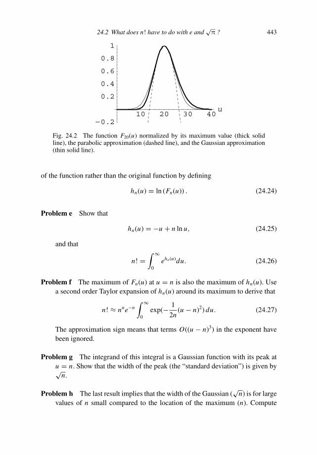
24.2 What does n! have to do with e and√
π ? 443
10 20 30 40u
−0.2
0.2
0.4
0.6
0.8
1
Fig. 24.2 The function F20(u) normalized by its maximum value (thick solidline), the parabolic approximation (dashed line), and the Gaussian approximation(thin solid line).
of the function rather than the original function by defining
hn(u) = ln (Fn(u)) . (24.24)
Problem e Show that
hn(u) = −u + n ln u, (24.25)
and that
n! =∫ ∞
0ehn(u)du. (24.26)
Problem f The maximum of Fn(u) at u = n is also the maximum of hn(u). Usea second order Taylor expansion of hn(u) around its maximum to derive that
n! ≈ nne−n∫ ∞
0exp(− 1
2n(u − n)2) du. (24.27)
The approximation sign means that terms O((u − n)3) in the exponent havebeen ignored.
Problem g The integrand of this integral is a Gaussian function with its peak atu = n. Show that the width of the peak (the “standard deviation”) is given by√
n.
Problem h The last result implies that the width of the Gaussian (√
n) is for largevalues of n small compared to the location of the maximum (n). Compute

444 Asymptotic evaluation of integrals
the value of the Gaussian function at the lower end of the integration interval(u = 0) for n = 5, 10, and 100, respectively.
The integral (24.27) runs from u = 0 to u = ∞. If the integration ran fromu = −∞ to u = ∞ then we could solve the integral using
∫ ∞
−∞e−ax2
dx =√
π
a. (24.28)
However, as shown in Figure 24.2 the integrand in (24.27) is for large values ofn small for negative values of u. Also, as shown in the last problem, even formoderately large values of n, the integrand is extremely small at the integrationboundary u = 0. For this reason, we make a small error by extending the integrationlimit in (24.27) to −∞:
n! ≈ nne−n∫ ∞
−∞exp(− 1
2n(u − n)2) du. (24.29)
Problem i Use the Gaussian integral (24.28) to show that
n! ≈ nne−n√
2πn. (24.30)
This approximation is called Stirling’s formula. In this expression the meaningof the ≈ sign is not precise. In the derivation of (24.30) we have made two approx-imations; the second order Taylor approximation of problem f and the extension ofthe lower limit of the integral (24.27) from 0 to −∞. The first approximation can beimproved by using a higher-order Taylor approximation, while the second approx-imation can be improved by using an asymptotic expansion of the error functionas presented in the previous section. A more detail analysis of this problem showsthat n! can be written as [14]:
n! ≈ nne−n√
2πn(
1 + c1
n+ c2
n2+ · · ·
)
. (24.31)
This series behaves differently to the series we have encountered so far since it hasthe following properties [14]:
For small n the cn decrease with increasing values of n. However, for larger values ofn the cn increase so rapidly with n that the series diverges. Trying to sum the seriestherefore is pointless.
When the series is truncated at a certain point, the truncated series becomes more andmore accurate as n increases.
For a given value of n there is an optimal truncation point.
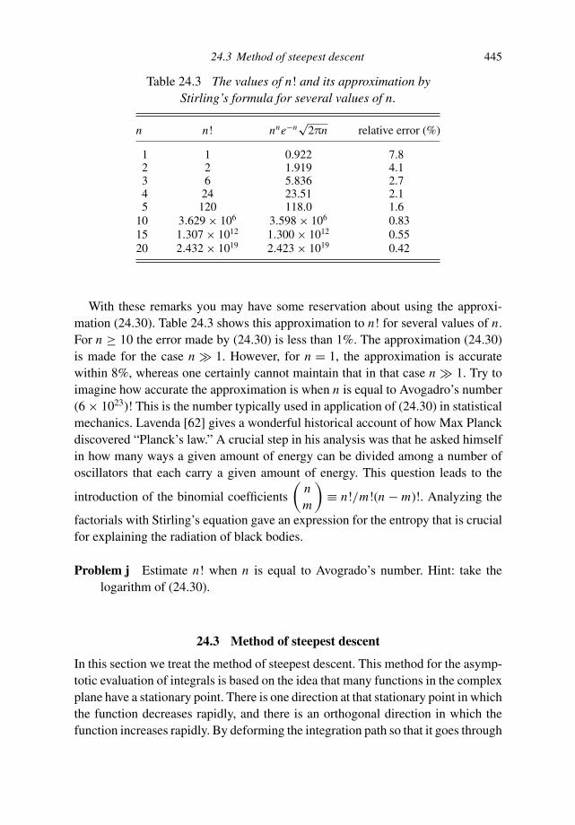
24.3 Method of steepest descent 445
Table 24.3 The values of n! and its approximation byStirling’s formula for several values of n.
n n! nne−n√
2πn relative error (%)
1 1 0.922 7.82 2 1.919 4.13 6 5.836 2.74 24 23.51 2.15 120 118.0 1.6
10 3.629 × 10⁶ 3.598 × 10⁶ 0.8315 1.307 × 10¹² 1.300 × 10¹² 0.5520 2.432 × 10¹⁹ 2.423 × 10¹⁹ 0.42
With these remarks you may have some reservation about using the approxi-mation (24.30). Table 24.3 shows this approximation to n! for several values of n.For n ≥ 10 the error made by (24.30) is less than 1%. The approximation (24.30)is made for the case n 1. However, for n = 1, the approximation is accuratewithin 8%, whereas one certainly cannot maintain that in that case n 1. Try toimagine how accurate the approximation is when n is equal to Avogadro’s number(6 × 10²³)! This is the number typically used in application of (24.30) in statisticalmechanics. Lavenda [62] gives a wonderful historical account of how Max Planckdiscovered “Planck’s law.” A crucial step in his analysis was that he asked himselfin how many ways a given amount of energy can be divided among a number ofoscillators that each carry a given amount of energy. This question leads to the
introduction of the binomial coefficients
(
nm
)
≡ n!/m!(n − m)!. Analyzing the
factorials with Stirling’s equation gave an expression for the entropy that is crucialfor explaining the radiation of black bodies.
Problem j Estimate n! when n is equal to Avogrado’s number. Hint: take thelogarithm of (24.30).
24.3 Method of steepest descent
In this section we treat the method of steepest descent. This method for the asymp-totic evaluation of integrals is based on the idea that many functions in the complexplane have a stationary point. There is one direction at that stationary point in whichthe function decreases rapidly, and there is an orthogonal direction in which thefunction increases rapidly. By deforming the integration path so that it goes through

446 Asymptotic evaluation of integrals
x
Fig. 24.3 The function e(
exp(
i x2))
for −6 < x < 6. The vertical axis runsfrom −1 to 1.
−4−2
0
2
4
x
−4−2
0
2
4
y
02
4
−20
2
Fig. 24.4 The function e(
exp(
i z2))
in the complex plane. For clarity the expo-nential growth has been modified by plotting the function e−0.1×2xy cos(x2 − y2).
the stationary point in the direction in which the function decreases, one can eval-uate the integral asymptotically. As an example we apply this idea to the followingintegral
I =∫ ∞
−∞eiax2
dx, with a > 0. (24.32)
Let us first investigate the behavior of the integrand exp(
i z2)
in the complexplane with z = x + iy for the special case a = 1. The real part of the integrandalong the real axis is shown in Figure 24.3. Along this axis, the integrand is arapidly oscillating function, except near the point x = 0 where the function isstationary. The real part of exp
(
i z2)
in the complex plane is shown in Figure 24.4.It can be seen from this figure that along the real axis and along the imaginary axis,the function is oscillatory. Along the line y = x the function has a maximum at the

24.3 Method of steepest descent 447
−2 −1 1 2r
1
2
3
4
5
Fig. 24.5 The function e(
exp(
i z2))
in the complex plane along the lines x = y(solid line) and x = −y (dashed line).
osci
llato
ry
x
y
steep
est d
esce
nt
steepest ascent
f oscillatory
Fig. 24.6 The behaviour of the function eiz2in the complex plane.
origin, while along the line y = −x the function has a minimum at the origin. Thebehavior of e
(
exp(
i z2))
along these lines is shown in Figure 24.5.
Problem a Compute e(
exp(
i z2))
along the x-axis, the y-axis, and the linesy = ±x and show that this function has a behavior as shown in Figure 24.6. Adirection of steepest descent means that in that direction the function decreasesfrom its stationary point, while a direction of steepest ascent means that in thatdirection a function increases from its stationary point.
There is a good reason why there are steepest descent and steepest ascent direc-tions that are perpendicular. As shown in Section 16.1, the real and imaginary partsof an analytic function satisfy Laplace’s equation: ∇2 f = 0. Let us momentarily
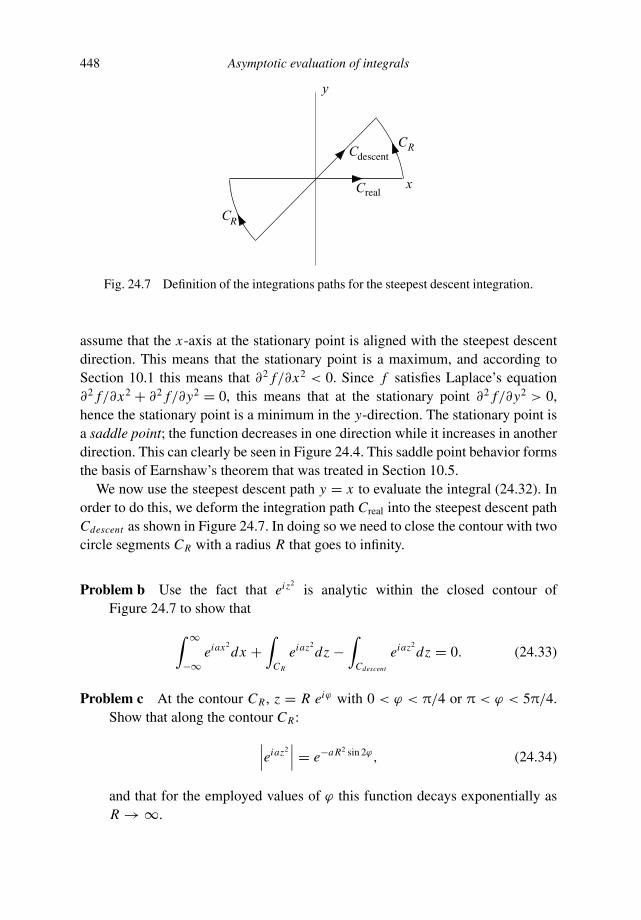
448 Asymptotic evaluation of integrals
x
y
CR
CR
Creal
Cdescent
Fig. 24.7 Definition of the integrations paths for the steepest descent integration.
assume that the x-axis at the stationary point is aligned with the steepest descentdirection. This means that the stationary point is a maximum, and according toSection 10.1 this means that ∂2 f/∂x2 < 0. Since f satisfies Laplace’s equation∂2 f/∂x2 + ∂2 f/∂y2 = 0, this means that at the stationary point ∂2 f/∂y2 > 0,hence the stationary point is a minimum in the y-direction. The stationary point isa saddle point; the function decreases in one direction while it increases in anotherdirection. This can clearly be seen in Figure 24.4. This saddle point behavior formsthe basis of Earnshaw’s theorem that was treated in Section 10.5.
We now use the steepest descent path y = x to evaluate the integral (24.32). Inorder to do this, we deform the integration path Creal into the steepest descent pathCdescent as shown in Figure 24.7. In doing so we need to close the contour with twocircle segments CR with a radius R that goes to infinity.
Problem b Use the fact that eiz2is analytic within the closed contour of
Figure 24.7 to show that
∫ ∞
−∞eiax2
dx +∫
CR
eiaz2dz −
∫
Cdescent
eiaz2dz = 0. (24.33)
Problem c At the contour CR , z = R eiϕ with 0 < ϕ < π/4 or π < ϕ < 5π/4.Show that along the contour CR:
∣
∣
∣eiaz2∣
∣
∣ = e−a R2 sin 2ϕ, (24.34)
and that for the employed values of ϕ this function decays exponentially asR → ∞.

24.3 Method of steepest descent 449
This result implies that the contribution of the contours CR vanishes as R → ∞,so that according to (24.33):
∫ ∞
−∞eiax2
dx =∫
Cdescent
eiaz2dz. (24.35)
Problem d Evaluate the integral on the right-hand side by substituting z = ueiπ/4
and use (24.28) to show that∫ ∞
−∞eiax2
dx =√
π
aeiπ/4 (a > 0). (24.36)
Problem e Show that this result can also be obtained by simply substitutingb = −ia into the integral (24.28). This substitution does not address anyconvergence issues of the resulting integral. However, it is a simple trick tomemorize (24.36).
Problem f Repeat the analysis that leads to problem d for a < 0. Show thatin this case the steepest descent direction is along the line y = −x andthat
∫ ∞
−∞eiax2
dx =√
π
|a| e−iπ/4 (a < 0). (24.37)
Note that the expressions (24.36) and (24.37) can be summarized by the singleexpression
∫ ∞
−∞eiax2
dx =√
π
|a|eiπ/4 sgn(a), (24.38)
with
sgn(a) ≡⎧
⎨
⎩
+1 when a > 0
−1 when a < 0. (24.39)
The integration in this section was over a single variable. Bleistein and Handels-man [18] show how this analysis can be extended to multidimensional integrals:
∫
exp(ix · A · x)d N x =√
πN
|det A| eiπ/4 sgn(A), (24.40)
where sgn(A) = number of positive eigenvalues of A− number of negative eigen-values of A.
450 Asymptotic evaluation of integrals
The advantage of using expression (24.38) is that we do not need to know thesteepest descent path once we know this integral. The integral (24.38) forms thebasis of the method of stationary phase that will be treated in the next section. Sincethe method of stationary phase uses the original integration path along the real axis,one can say that the method of stationary phase is the steepest descent method forthose that are too lazy to deform contours in the complex plane.
24.4 Group velocity and the method of stationary phase
Before treating the method of stationary phase, let us briefly examine a commonexplanation of the concept of group velocity. Suppose a wave consists of twopropagating waves of equal amplitudes with frequencies ω1 and ω2 that are close:
p(x, t) = cos(k(ω1)x − ω1t) + cos(k(ω2)x − ω2t) (24.41)
Note that the wave number is a function of frequency: k = k(ω). In the followingwe use
ω1 = ω0 − ∆ and ω2 = ω0 + ∆, (24.42)
so that ω0 is the center frequency and 2 the frequency separation.
Problem a Use a first-order Taylor expansion of k(ω) around the point ω0 to showthat
cos(k(ω1)x − ω1t) = cos(k0x − ω0t) cos
(
∆
(
∂k
∂ωx − t
))
+ sin(k0x − ω0t) sin
(
∆
(
∂k
∂ωx − t
))
,
(24.43)
where k0 = k(ω0) and ∂k/∂ω is evaluated at ω0.
Problem b Apply the same analysis to the last term of (24.41) and derive that
p(x, t) = 2 cos(
ω0(t − x
c))
cos(
∆
(
t − x
U
))
, (24.44)
with
c = ω
kand U = ∂ω
∂k. (24.45)
Since ∆ ω0, the total wave field (24.44) consists of a wave cos(ω0(t − (x/c)))that propagates with a velocity c that is modulated by a slowly varying amplitudevariation cos(∆(t − x/U )) that propagates with a velocity U . The velocity U of

24.4 Group velocity and the method of stationary phase 451
the amplitude variation is called the group velocity, while the velocity c with whichthe carrier wave of frequency ω0 propagates is called the phase velocity.
Even though this analysis is relatively simple, it is not very realistic. A propagat-ing wave rarely consists of two frequency components that have equal amplitudes.In general, a wave consists of the superposition of all frequency components withina certain frequency band, and the amplitude spectrum A(ω) in general is not aconstant. In the frequency domain such a wave is given by A(ω) exp(ik(ω)x), andafter a Fourier transform the wave is in the time domain given by
p(x, t) =∫ ∞
−∞A(ω)ei(k(ω)x−ωt)dω. (24.46)
In the following we assume that the amplitude A(ω) varies slowly with frequencycompared to the phase
ψ(ω) = k(ω)x − ωt. (24.47)
In general, the phase is a rapidly oscillating function of frequency. We argued inthe previous section that the dominant contribution to the integral
∫ ∞−∞ eiax2
dx camefrom the saddle point x = 0. In Figure 24.3 the saddle point x = 0 corresponds tothe point where the function ceases to oscillate. This corresponds to the point wherethe phase in the exponent is stationary, that is this is the point where the phase iseither a maximum or a minimum. For the function eiax2
the phase is given by ax2,the phase is stationary when d
(
ax2)
/dx = 0; this implies that x = 0, which isindeed the point of stationary phase in Figure 24.3.
Problem c Show that the phase (24.47) is stationary when
∂k
∂ωx − t = 0. (24.48)
With the definition (24.45) for the group velocity this result can also be written as
U (ω0) = x
t. (24.49)
Before we proceed, let us briefly reflect on this result. The Fourier integral (24.46)states that all frequencies contribute to the wave field. However, for given valuesof x and t the dominant contribution to this frequency integral comes from thefrequency ω0 for which the phase of the integrand is stationary. This frequency isdefined by expression (24.49). When the group velocity is known as a function offrequency, this expression implicitly defines ω0. Note that this frequency dependson the location x and the time t for which we want to compute the wave field. Theright-hand side x/t is the distance x covered in a time t , the principle of stationary
452 Asymptotic evaluation of integrals
phase simply states that this distance is covered with a velocity given by the groupvelocity.
We approximate the integral (24.46) here with the method of stationary phase.In this approximation we assume that:
The amplitude A(ω) varies slowly with ω, so that we can replace the amplitude by itsvalue at the stationary point:
A(ω) ≈ A(ω0). (24.50)
For the phase we use a second order Taylor expansion around the stationary point:
ψ(ω) ≈ ψ(ω0) + 1
2
∂2ψ
∂ω2(ω − ω0)2, (24.51)
where the second derivative is evaluated at the stationary point ω0. Note that the firstderivative does not appear in this Taylor expansion because at the stationary point wehave by definition that ∂ψ/∂ω = 0.
Insert these approximations into (24.46) and evaluate the remaining integral with expres-sion (24.38).
Problem d The first step in this approach is trivial. In the second step we need∂2ψ/∂ω2 at the stationary point. Compute this derivative and use (24.45) toshow that
∂2ψ
∂ω2= ∂2k
∂ω2x = − 1
U 2
∂U
∂ωx, (24.52)
where all quantities are evaluated at frequency ω0.
Problem e Insert (24.50)–(24.52) into the integral (24.46) and solve the remainingintegral with (24.38) to show that
p(x, t) ≈ A(ω0)ei(k0x−ω0t)
√
2π
|∂U/∂ω| xU (ω0)e−iπ/4 sgn(∂U/∂ω). (24.53)
This expression generalizes (24.44) for a wave with an arbitrary amplitude spec-trum A(ω). The wave (24.53) consists of a carrier wave exp(i(k0x − ω0t)) withamplitude A(ω0). The frequency ω0 is determined by the condition that the groupvelocity U (ω0) is the velocity needed to cover the distance x in time t . The ampli-tude of the wave is also determined by the term 1/
√|∂U/∂ω| x . Let us first considerthe x-dependence. The wave we consider here has a group velocity that dependson frequency. This means that the different frequency components travel with adifferent velocity. Because of this, the amplitude of the wave is reduced as the

24.5 Asymptotic behavior of the Bessel function J0(x) 453
wave propagates, because the different frequency components are spread-out overspace during the propagation. This phenomenon is called dispersion. The decayof the amplitude with propagation distance is given by the term 1/
√x . Suppose
that the group velocity depends weakly on frequency. In that case ∂U/∂ω is small.In that situation, many different frequency components interfere constructively inthe Fourier integral. This leads to a large amplitude that is described by the term1/
√|∂U/∂ω|. An extensive treatment of the concept of group velocity is given byBrillouin [21].
An example of wave dispersion can be seen in Figure 20.11 which shows thevertical component of the ground motion recorded in Belarus after an earthquake atJan-Mayen Island. Between t = 650 s and t = 900 s a dispersive wave arrives. Thisis the Rayleigh wave, an elastic wave that is guided along the Earth’s surface. Thefrequency content at early times (t = 700 s) is lower than at later times (say t =800 s). This dispersion is caused by the fact that the group velocity of the Rayleighwave decreases with increasing frequency for the frequencies that contribute to theseismogram in Figure 20.11. This causes the low-frequency components to arriveearlier than the high-frequency components.
It may occur that the group velocity does not depend on frequency. Accordingto (24.52) this means that ∂2ψ/∂ω2 = 0 and the stationary phase integral (24.53)is infinite. In that case the Taylor expansion (24.51) must be replaced by the thirdorder Taylor expansion
ψ(ω) ≈ ψ(ω0) + 1
6
∂3ψ
∂ω3(ω − ω0)3. (24.54)
The resulting integral can be integrated to give an Airy function [14]. The corre-sponding wave arrivals are called Airy phases [114]; these waves have, in general,a strong amplitude because many different frequency components interfere con-structively.
24.5 Asymptotic behavior of the Bessel function J0(x)
In Section 20.5 we showed that for x n the Bessel function Jn(x) behaves as adecaying cosine:
Jn(x) ≈ A√x
cos (x + ϕ) . (24.55)
This relation followed from an analysis of the differential equation of the Besselfunction for large values of x . The analysis of Section 20.5 did not tell us whatthe constants A and ϕ are. Here we find these constants for J0(x) by applyinga stationary phase analysis to the following integral representation of the Bessel

454 Asymptotic evaluation of integrals
function:
J0(x) = 1
π
∫ π
0cos (x sin ϕ) dϕ. (24.56)
Before we solve this integral in the stationary phase approximation, let us verifythat this is a valid representation of the Bessel function. In order to do this, we needto check if the representation (24.56) satisfies the Bessel equation (20.16), with thefollowing initial conditions:
J0(x = 0) = 1,d J0
dx(x = 0) = 0. (24.57)
Problem a Show that
d J0
dx= −1
π
∫ π
0sin (x sin ϕ) sin ϕ dϕ, (24.58)
and
d2 J0
dx2= −1
π
∫ π
0cos (x sin ϕ) sin2 ϕ dϕ. (24.59)
Using the identity sin2 ϕ = 1 − cos2 ϕ, the last integral can be written as−π−1
∫ π0 cos (x sin ϕ) dϕ + π−1
∫ π0 cos (x sin ϕ) cos2 ϕ dϕ. In the last term we can
use that
cos(x sin ϕ) = 1
x cos ϕ
d sin(x sin ϕ)
dϕ. (24.60)
Problem b Insert these results into (24.59), and use an integration by parts of thelast term to derive that
d2 J0
dx2= −1
π
∫ π
0cos (x sin ϕ) dϕ + 1
πx
∫ π
0sin (x sin ϕ) sin ϕ dϕ. (24.61)
Problem c Use this result with (24.56) and (24.58) to show that the representation(24.56) satisfies the Bessel equation (20.16).
Problem d We next check if J0(x) indeed satisfies the initial conditions (24.57).Apply the Taylor approximation technique of Section 24.1 to the integral(24.56) and show that for small values of x :
J0(x) = 1 + 0 · x + O(x2). (24.62)
24.5 Asymptotic behavior of the Bessel function J0(x) 455
This result implies that the initial conditions (24.57) are satisfied, so that(24.56) indeed is a valid representation of the Bessel function J0(x).
In order to apply a stationary phase analysis for x 1 to (24.56) we first rewriteit in the following form:
J0(x) = 1
πe
∫ π
0eixψ(ϕ)dϕ, (24.63)
with
ψ(ϕ) = sin ϕ. (24.64)
Problem e Show that the phase ψ is stationary for ϕ = π/2 and that at that pointd2ψ/dϕ2 = −1.
Problem f Use a second order Taylor expansion around the stationary point torewrite (24.63) as
J0(x) ≈ 1
πe eix
∫ π
0exp
(
− i x
2(ϕ − π
2)2
)
dϕ. (24.65)
The integrand has the behavior shown in Figure 24.3; away from the stationarypoint the integrand fluctuates rapidly and the positive contributions are canceled bythe negative contributions so that the dominant contribution to the integral comesfrom a region near the stationary point.
Problem g We can estimate the region of stationary phase by finding the valuesof ϕ for which the real part of the integrand of (24.65) vanishes. These pointscorrespond to the zero crossing in Figure 24.3 closest to the stationary point.Show that the corresponding values of ϕ are given by
ϕ = π
2±
√
π
x. (24.66)
For x 1 these values of ϕ are close to the stationary point. Since the dominantcontribution to the stationary phase integral (24.65) comes from the region close tothe stationary point, we can extend the integration interval to infinity:
J0(x) ≈ 1
πe eix
∫ ∞
−∞exp
(
− i x
2(ϕ − π
2)2
)
dϕ. (24.67)
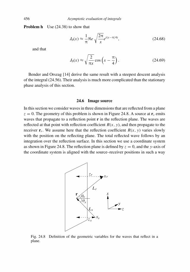
456 Asymptotic evaluation of integrals
Problem h Use (24.38) to show that
J0(x) ≈ 1
πe
√
2π
xei(x−π/4), (24.68)
and that
J0(x) ≈√
2
πxcos
(
x − π
4
)
. (24.69)
Bender and Orszag [14] derive the same result with a steepest descent analysisof the integral (24.56). Their analysis is much more complicated than the stationaryphase analysis of this section.
24.6 Image source
In this section we consider waves in three dimensions that are reflected from a planez = 0. The geometry of this problem is shown in Figure 24.8. A source at rs emitswaves that propagate to a reflection point r in the reflection plane. The waves arereflected at that point with reflection coefficient R(x, y), and then propagate to thereceiver rr . We assume here that the reflection coefficient R(x, y) varies slowlywith the position on the reflecting plane. The total reflected wave follows by anintegration over the reflection surface. In this section we use a coordinate systemas shown in Figure 24.8. The reflection plane is defined by z = 0, and the y-axis ofthe coordinate system is aligned with the source–receiver positions in such a way
x
yz
r
z s
Ls
s
r
Lr
zr x r
xs
Fig. 24.8 Definition of the geometric variables for the waves that reflect in aplane.

24.6 Image source 457
that:
rs =⎛
⎝
xs
0zs
⎞
⎠, r =⎛
⎝
xy0
⎞
⎠, rr =⎛
⎝
xr
0zr
⎞
⎠ . (24.70)
The propagation of the waves from the source to the reflection point, and from thereflection point to the receiver is given by the Green’s function (19.37) for scalarwaves in a 3D homogeneous medium. The total wave field is given by the integralover the reflecting plane, so that
p(rr ) =∞∫∫
−∞G(|rr − r|)R(x, y)G(|r − rs |) dxdy, (24.71)
with G given by expression (19.37).
Problem a Show that this integral can be written as
p(rr ) =∞∫∫
−∞A(x, y)R(x, y)eikψ(x,y)dxdy, (24.72)
with
A(x, y) = 1
(4π)2
(
(xr − x)2 + y2 + z2r
)−1/2 (
(xs − x)2 + y2 + z2s
)−1/2, (24.73)
and
ψ(x, y) =√
(xr − x)2 + y2 + z2r +
√
(xs − x)2 + y2 + z2s (24.74)
Problem b We will solve the integral (24.72) in the stationary phase approxi-mation. In order to do this we evaluate both the x- and the y-integral with astationary phase approximation. Before we can do this, we first need to findthe stationary point in the x, y-plane. In order to find this point, show first that
∂ψ
∂x= x − xr
√
(xr − x)2 + y2 + z2r
+ x − xs√
(xs − x)2 + y2 + z2s
, (24.75)
and
∂ψ
∂y= y
√
(xr − x)2 + y2 + z2r
+ y√
(xs − x)2 + y2 + z2s
. (24.76)

458 Asymptotic evaluation of integrals
Problem c At the stationary point, both derivatives vanish; show that the station-ary point is given by
x − xr
Lr+ x − xs
Ls= 0 and y = 0, (24.77)
with Lr and Ls defined in Figure 24.8.
Let us first analyze this stationary phase condition. The condition y = 0 statesthat the line from the source to the reflection point and the line from the reflectionpoint to the receiver lie in the same plane. The phase is thus stationary for in-planereflection. The first equality in (24.77) states for which point in that plane the phaseis stationary.
Problem d Use the angles θ s and θ r defined in Figure 24.8 to show that the pointof stationary phase as defined by the first equality in (24.77) satisfies
θ s = θ r . (24.78)
This identity implies that at the point of stationary phase the angles of the incomingand the outgoing waves are equal. If the waves could be described by rays, thereflection point would be defined by (24.78) and also the condition y = 0. Thecondition of stationary phase thus gives the same reflection point as would begiven by ray theory. A similar condition holds when the incoming and outgoingwaves travel at a different velocity. Snieder [97] shows that for the reflection ofsurface waves where the incoming surface wave mode travels with velocity cin andthe outgoing surface wave mode with velocity cout the point of stationary phasesatisfies
sin θ in
cin= sin θout
cout. (24.79)
This is nothing but Snell’s law [3, 53] for mode-converted waves.The condition of stationarity thus gives us the location of the ray-geometric
reflection point. Let is now compute the reflected wavefield. In order to evaluate(24.72) in the stationary phase approximation we need the second derivatives ofthe phase.
Problem e Show for an arbitrary point (x, y) that
∂2ψ
∂x2= y2 + z2
r(
(xr − x)2 + y2 + z2r
)3/2 + y2 + z2s
(
(xs − x)2 + y2 + z2s
)3/2 , (24.80)

24.6 Image source 459
and
∂2ψ
∂y2= (xr − x)2 + z2
r(
(xr − x)2 + y2 + z2r
)3/2 + (xs − x)2 + z2s
(
(xs − x)2 + y2 + z2s
)3/2 . (24.81)
Problem f Show that at the stationary point:
∂2ψ
∂x2= cos2 θ
(
1
Lr+ 1
Ls
)
, (24.82)
and
∂2ψ
∂y2=
(
1
Lr+ 1
Ls
)
, (24.83)
where θ = θ r = θ s at the reflection point, and Ls and Lr are the distance fromthe reflection point to the source and receiver, respectively.
Problem g Show that near the reflection point the phase is approximately given by
ψ(x, y) ≈ Lr + Ls + 1
2cos2 θ
(
1
Lr+ 1
Ls
)
(x − xrefl)2
+ 1
2
(
1
Lr+ 1
Ls
)
(y − yrefl)2, (24.84)
with (xrefl, yrefl) the coordinates of the reflection point.
Problem h Show that the amplitude A near the reflection point is given by
A(x, y) = 1
(4π)2 Lr Ls. (24.85)
Problem g Evaluate the x and y integral in (24.72) each with the stationary phaseapproximation, and show that in this approximation
p(rr ) = rexp (ik(Lr + Ls))
4π(Lr + Ls), (24.86)
with
r = i R
2k cos θ. (24.87)
In this expression R is the reflection coefficient at the reflection point at anangle of incidence θ .
Apart from a minus sign, the term exp (ik(Lr + Ls)) /4π(Lr + Ls) =−G(Lr + Ls) is the Green’s function for a distance Lr + Ls . The wavefield (24.86)

460 Asymptotic evaluation of integrals
LsL s
Lr
xr
xs
r
virtualsource
realsource
Fig. 24.9 The position of a virtual source that is the mirror image of the realsource.
can therefore be interpreted as the wavefield generated by a virtual source that is themirror image of the original source in the reflector plane, see Figure 24.9. This cor-responding Green’s function G(Lr + Ls) is multiplied in (24.86) with an effectivereflection coefficient r that accounts for the net reflectivity of the reflection plane.The stationary phase approximation thus not only accounts for the ray-geometricreflection point, it also describes how the original source can be replaced by animage source at the other side of the reflection point.
25
Variational calculus
25.1 Designing a can
As an introduction to variational calculus we consider in this section the problemof designing a can. Suppose you want to make the can with a given amount of metalthat has the largest content. A squat can with a small height and a large radius hasa small volume, but a tall can with a large height but a small radius cannot containmuch either. Clearly there is a specific shape of the can that maximizes the volumefor a given surface area. Consider the can shown in Figure 25.1, the top and bottomeach having a surface area S, the height denoted by h, and the circumference of thecan denoted by C . The total surface area A is twice the surface area of the bottom,plus the surface area hC of the side, so that
A = 2S + hC. (25.1)
The volume V of the can is the product of the surface area of the bottom times theheight:
V = hS. (25.2)
Problem a We want to eliminate the height h from the problem. Use expression(25.1) to show that
h = (A − 2S)
C, (25.3)
and use this result to show that
V = (A − 2S) S
C. (25.4)
Problem b For the moment we assume that the can has the shape of cylinder withradius r . Express the surface area S and the circumference C in this radius,
461
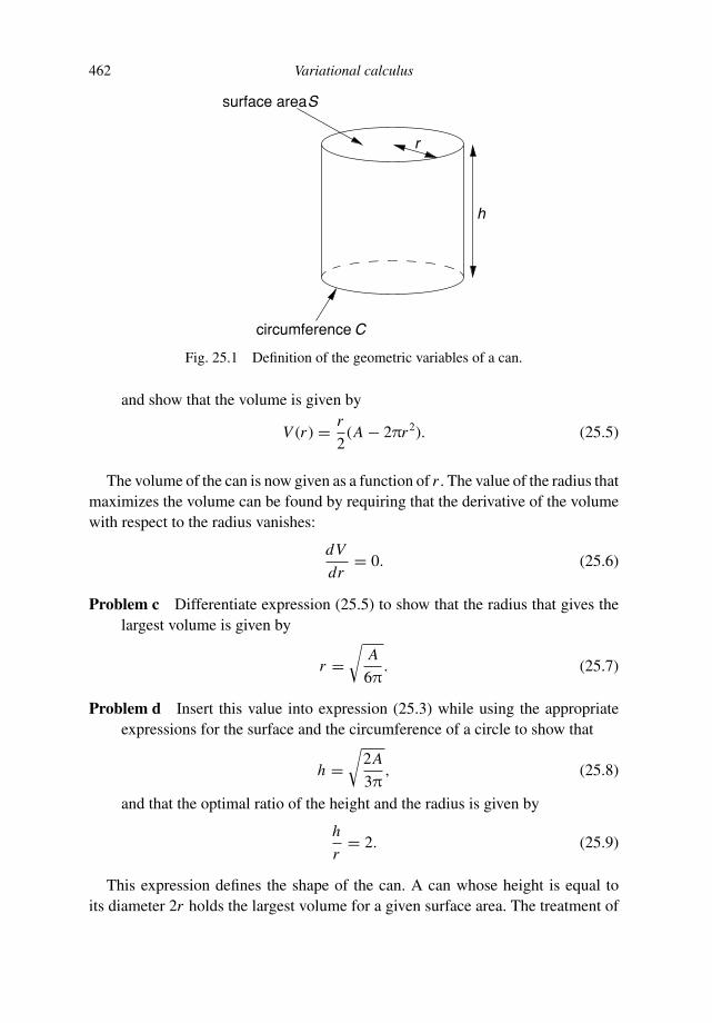
462 Variational calculus
r
h
surface area S
circumference C
Fig. 25.1 Definition of the geometric variables of a can.
and show that the volume is given by
V (r ) = r
2(A − 2πr2). (25.5)
The volume of the can is now given as a function of r . The value of the radius thatmaximizes the volume can be found by requiring that the derivative of the volumewith respect to the radius vanishes:
dV
dr= 0. (25.6)
Problem c Differentiate expression (25.5) to show that the radius that gives thelargest volume is given by
r =√
A
6π. (25.7)
Problem d Insert this value into expression (25.3) while using the appropriateexpressions for the surface and the circumference of a circle to show that
h =√
2A
3π, (25.8)
and that the optimal ratio of the height and the radius is given by
h
r= 2. (25.9)
This expression defines the shape of the can. A can whose height is equal toits diameter 2r holds the largest volume for a given surface area. The treatment of
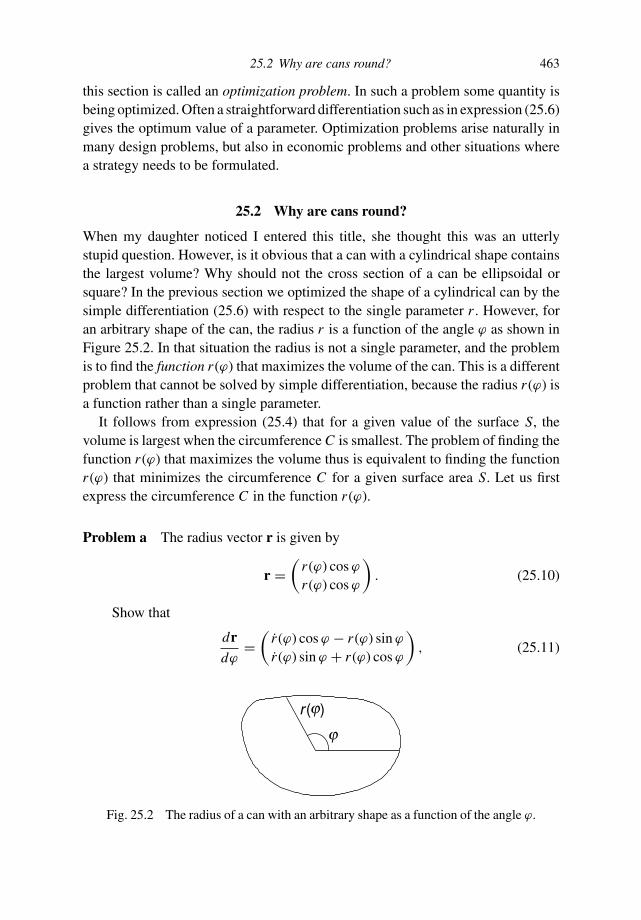
25.2 Why are cans round? 463
this section is called an optimization problem. In such a problem some quantity isbeing optimized. Often a straightforward differentiation such as in expression (25.6)gives the optimum value of a parameter. Optimization problems arise naturally inmany design problems, but also in economic problems and other situations wherea strategy needs to be formulated.
25.2 Why are cans round?
When my daughter noticed I entered this title, she thought this was an utterlystupid question. However, is it obvious that a can with a cylindrical shape containsthe largest volume? Why should not the cross section of a can be ellipsoidal orsquare? In the previous section we optimized the shape of a cylindrical can by thesimple differentiation (25.6) with respect to the single parameter r . However, foran arbitrary shape of the can, the radius r is a function of the angle ϕ as shown inFigure 25.2. In that situation the radius is not a single parameter, and the problemis to find the function r (ϕ) that maximizes the volume of the can. This is a differentproblem that cannot be solved by simple differentiation, because the radius r (ϕ) isa function rather than a single parameter.
It follows from expression (25.4) that for a given value of the surface S, thevolume is largest when the circumference C is smallest. The problem of finding thefunction r (ϕ) that maximizes the volume thus is equivalent to finding the functionr (ϕ) that minimizes the circumference C for a given surface area S. Let us firstexpress the circumference C in the function r (ϕ).
Problem a The radius vector r is given by
r =(
r (ϕ) cos ϕ
r (ϕ) cos ϕ
)
. (25.10)
Show that
drdϕ
=(
r (ϕ) cos ϕ − r (ϕ) sin ϕ
r (ϕ) sin ϕ + r (ϕ) cos ϕ
)
, (25.11)
jr (j)
Fig. 25.2 The radius of a can with an arbitrary shape as a function of the angle ϕ.
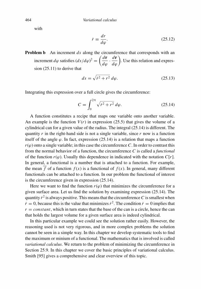
464 Variational calculus
with
r ≡ dr
dϕ. (25.12)
Problem b An increment ds along the circumference that corresponds with an
increment dϕ satisfies (ds/dϕ)2 =(
drdϕ
· drdϕ
)
. Use this relation and expres-
sion (25.11) to derive that
ds =√
r2 + r2 dϕ. (25.13)
Integrating this expression over a full circle gives the circumference:
C =∫ 2π
0
√
r2 + r2 dϕ. (25.14)
A function constitutes a recipe that maps one variable onto another variable.An example is the function V (r ) in expression (25.5) that gives the volume of acylindrical can for a given value of the radius. The integral (25.14) is different. Thequantity r in the right-hand side is not a single variable, since r now is a functionitself of the angle ϕ. In fact, expression (25.14) is a relation that maps a functionr (ϕ) onto a single variable; in this case the circumference C . In order to contrast thisfrom the normal behavior of a function, the circumference C is called a functionalof the function r (ϕ). Usually this dependence in indicated with the notation C[r ].In general, a functional is a number that is attached to a function. For example,the mean f of a function f (x) is a functional of f (x). In general, many differentfunctionals can be attached to a function. In our problem the functional of interestis the circumference given in expression (25.14).
Here we want to find the function r (ϕ) that minimizes the circumference for agiven surface area. Let us find the solution by examining expression (25.14). Thequantity r2 is always positive. This means that the circumference C is smallest whenr = 0, because this is the value that minimizes r2. The condition r = 0 implies thatr = constant , which in turn states that the base of the can is a circle, hence the canthat holds the largest volume for a given surface area is indeed cylindrical.
In this particular example we could see the solution rather easily. However, thereasoning used is not very rigorous, and in more complex problems the solutioncannot be seen in a simple way. In this chapter we develop systematic tools to findthe maximum or minium of a functional. The mathematics that is involved is calledvariational calculus. We return to the problem of minimizing the circumference inSection 25.9. In this chapter we cover the basic principles of variational calculus.Smith [95] gives a comprehensive and clear overview of this topic.
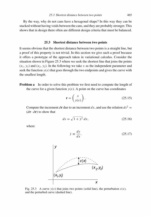
25.3 Shortest distance between two points 465
By the way, why do not cans have a hexagonal shape? In this way they can bestacked without having voids between the cans, and they are probably stronger. Thisshows that in design there often are different design criteria that must be balanced.
25.3 Shortest distance between two points
It seems obvious that the shortest distance between two points is a straight line, buta proof of this property is not trivial. In this section we give such a proof becauseit offers a prototype of the approach taken in variational calculus. Consider thesituation shown in Figure 25.3 where we seek the shortest line that joins the points(x1, y1) and (x2, y2). In the following we take x as the independent parameter andseek the function y(x) that goes through the two endpoints and gives the curve withthe smallest length.
Problem a In order to solve this problem we first need to compute the length ofthe curve for a given function y(x). A point on the curve has coordinates
r =(
xy(x)
)
. (25.15)
Compute the increment dr due to an increment dx , and use the relation ds2 =(dr · dr) to show that
ds =√
1 + y2 dx, (25.16)
where
y ≡ dy
dx. (25.17)
y
x
e(x)
(x ,y )1 1
(x ,y )2 2
Fig. 25.3 A curve y(x) that joins two points (solid line), the perturbation ε(x),and the perturbed curve (dashed line).
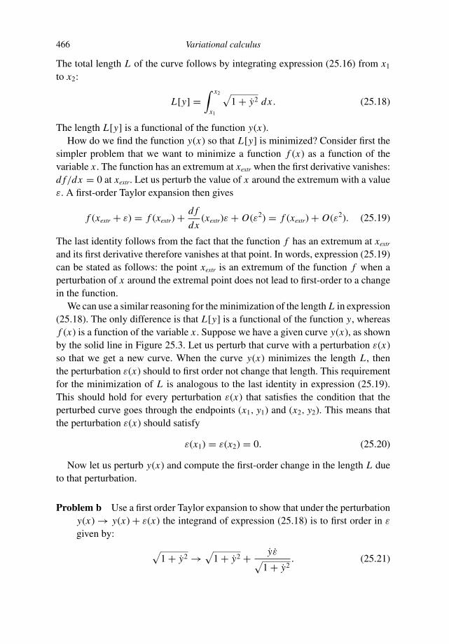
466 Variational calculus
The total length L of the curve follows by integrating expression (25.16) from x1
to x2:
L[y] =∫ x2
x1
√
1 + y2 dx . (25.18)
The length L[y] is a functional of the function y(x).How do we find the function y(x) so that L[y] is minimized? Consider first the
simpler problem that we want to minimize a function f (x) as a function of thevariable x . The function has an extremum at xextr when the first derivative vanishes:d f/dx = 0 at xextr. Let us perturb the value of x around the extremum with a valueε. A first-order Taylor expansion then gives
f (xextr + ε) = f (xextr) + d f
dx(xextr)ε + O(ε2) = f (xextr) + O(ε2). (25.19)
The last identity follows from the fact that the function f has an extremum at xextr
and its first derivative therefore vanishes at that point. In words, expression (25.19)can be stated as follows: the point xextr is an extremum of the function f when aperturbation of x around the extremal point does not lead to first-order to a changein the function.
We can use a similar reasoning for the minimization of the length L in expression(25.18). The only difference is that L[y] is a functional of the function y, whereasf (x) is a function of the variable x . Suppose we have a given curve y(x), as shownby the solid line in Figure 25.3. Let us perturb that curve with a perturbation ε(x)so that we get a new curve. When the curve y(x) minimizes the length L , thenthe perturbation ε(x) should to first order not change that length. This requirementfor the minimization of L is analogous to the last identity in expression (25.19).This should hold for every perturbation ε(x) that satisfies the condition that theperturbed curve goes through the endpoints (x1, y1) and (x2, y2). This means thatthe perturbation ε(x) should satisfy
ε(x1) = ε(x2) = 0. (25.20)
Now let us perturb y(x) and compute the first-order change in the length L dueto that perturbation.
Problem b Use a first order Taylor expansion to show that under the perturbationy(x) → y(x) + ε(x) the integrand of expression (25.18) is to first order in ε
given by:
√
1 + y2 →√
1 + y2 + yε√
1 + y2. (25.21)
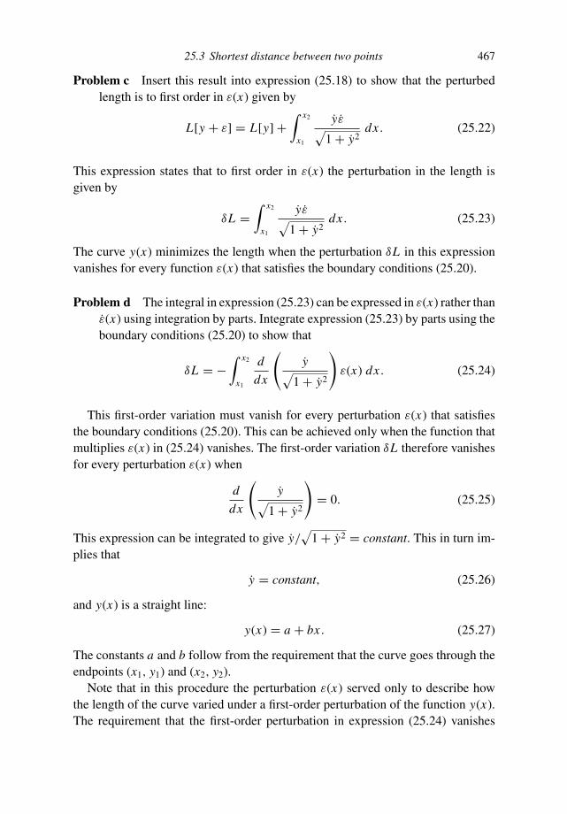
25.3 Shortest distance between two points 467
Problem c Insert this result into expression (25.18) to show that the perturbedlength is to first order in ε(x) given by
L[y + ε] = L[y] +∫ x2
x1
yε√
1 + y2dx . (25.22)
This expression states that to first order in ε(x) the perturbation in the length isgiven by
δL =∫ x2
x1
yε√
1 + y2dx . (25.23)
The curve y(x) minimizes the length when the perturbation δL in this expressionvanishes for every function ε(x) that satisfies the boundary conditions (25.20).
Problem d The integral in expression (25.23) can be expressed in ε(x) rather thanε(x) using integration by parts. Integrate expression (25.23) by parts using theboundary conditions (25.20) to show that
δL = −∫ x2
x1
d
dx
(
y√
1 + y2
)
ε(x) dx . (25.24)
This first-order variation must vanish for every perturbation ε(x) that satisfiesthe boundary conditions (25.20). This can be achieved only when the function thatmultiplies ε(x) in (25.24) vanishes. The first-order variation δL therefore vanishesfor every perturbation ε(x) when
d
dx
(
y√
1 + y2
)
= 0. (25.25)
This expression can be integrated to give y/√
1 + y2 = constant. This in turn im-plies that
y = constant, (25.26)
and y(x) is a straight line:
y(x) = a + bx . (25.27)
The constants a and b follow from the requirement that the curve goes through theendpoints (x1, y1) and (x2, y2).
Note that in this procedure the perturbation ε(x) served only to describe howthe length of the curve varied under a first-order perturbation of the function y(x).The requirement that the first-order perturbation in expression (25.24) vanishes
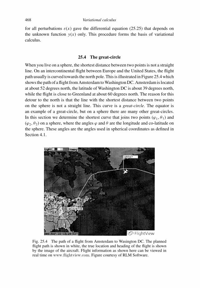
468 Variational calculus
for all perturbations ε(x) gave the differential equation (25.25) that depends onthe unknown function y(x) only. This procedure forms the basis of variationalcalculus.
25.4 The great-circle
When you live on a sphere, the shortest distance between two points is not a straightline. On an intercontinental flight between Europe and the United States, the flightpath usually is curved towards the north pole. This is illustrated in Figure 25.4 whichshows the path of a flight from Amsterdam to Washington DC. Amsterdam is locatedat about 52 degrees north, the latitude of Washington DC is about 39 degrees north,while the flight is close to Greenland at about 60 degrees north. The reason for thisdetour to the north is that the line with the shortest distance between two pointson the sphere is not a straight line. This curve is a great-circle. The equator isan example of a great-circle, but on a sphere there are many other great-circles.In this section we determine the shortest curve that joins two points (ϕ1, θ1) and(ϕ2, θ2) on a sphere, where the angles ϕ and θ are the longitude and co-latitude onthe sphere. These angles are the angles used in spherical coordinates as defined inSection 4.1.
Fig. 25.4 The path of a flight from Amsterdam to Wasington DC. The plannedflight path is shown in white, the true location and heading of the flight is shownby the image of the aircraft. Flight information as shown here can be viewed inreal time on www.flightview.com. Figure courtesy of RLM Software.
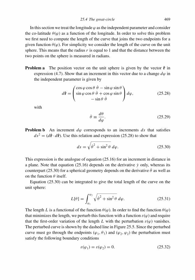
25.4 The great-circle 469
In this section we treat the longitude ϕ as the independent parameter and considerthe co-latitude θ (ϕ) as a function of the longitude. In order to solve this problemwe first need to compute the length of the curve that joins the two endpoints for agiven function θ (ϕ). For simplicity we consider the length of the curve on the unitsphere. This means that the radius r is equal to 1 and that the distance between thetwo points on the sphere is measured in radians.
Problem a The position vector on the unit sphere is given by the vector r inexpression (4.7). Show that an increment in this vector due to a change dϕ inthe independent parameter is given by
d r =⎛
⎝
cos ϕ cos θ θ − sin ϕ sin θ
sin ϕ cos θ θ + cos ϕ sin θ
− sin θ θ
⎞
⎠ dϕ, (25.28)
with
θ ≡ dθ
dϕ. (25.29)
Problem b An increment dϕ corresponds to an increments ds that satisfiesds2 = (d r · d r). Use this relation and expression (25.28) to show that
ds =√
θ2 + sin2 θ dϕ. (25.30)
This expression is the analogue of equation (25.16) for an increment in distance ina plane. Note that equation (25.16) depends on the derivative y only, whereas itscounterpart (25.30) for a spherical geometry depends on the derivative θ as well ason the function θ itself.
Equation (25.30) can be integrated to give the total length of the curve on theunit sphere:
L[θ ] =∫ ϕ2
ϕ1
√
θ2 + sin2 θ dϕ. (25.31)
The length L is a functional of the function θ (ϕ). In order to find the function θ (ϕ)that minimizes the length, we perturb this function with a function ε(ϕ) and requirethat the first-order variation of the length L with the perturbation ε(ϕ) vanishes.The perturbed curve is shown by the dashed line in Figure 25.5. Since the perturbedcurve must go through the endpoints (ϕ1, θ1) and (ϕ2, ϕ2) the perturbation mustsatisfy the following boundary conditions
ε(ϕ1) = ε(ϕ2) = 0. (25.32)

470 Variational calculus
e(f)
(f ,q )
(f ,q )
1
22
1
Fig. 25.5 The unperturbed curve θ (ϕ) that joins two points on the sphere (solidline), the perturbation ε(ϕ), and the perturbed curve (dashed line).
Problem c Show that under the perturbation θ → θ + ε the following first-orderperturbations hold:
θ2 → θ
2 + 2θ ε, (25.33)
sin θ → sin (θ + ε) = sin θ + ε cos θ, (25.34)
sin2 θ → sin2 θ + 2ε sin θ cos θ. (25.35)
Use these results to show that to first order in the perturbation ε the integrandof expression (25.31) is perturbed in the following way
√
θ2 + sin2 θ →
√
θ2 + sin2 θ + 2θ ε + ε sin 2θ
2√
θ2 + sin2 θ
. (25.36)
Integrating this expression between the endpoints ϕ1 and ϕ2 gives the followingfirst-order perturbation of the length due to the perturbation ε(ϕ):
δL = 1
2
∫ ϕ2
ϕ1
2θ ε + ε sin 2θ√
θ2 + sin2 θ
dϕ. (25.37)
Problem d This perturbation depends on both ε and ε. The derivative ε can beeliminated by carrying out an integration by parts of the first term of the

25.4 The great-circle 471
numerator using the boundary conditions (25.32). Use this to show that
δL = 1
2
∫ ϕ2
ϕ1
⎧
⎨
⎩
− d
dϕ
⎛
⎝
2θ√
θ2 + sin2 θ
⎞
⎠ + sin 2θ√
θ2 + sin2 θ
⎫
⎬
⎭
ε(ϕ) dϕ. (25.38)
For the curve that minimizes the distance, the length L is stationary and its firstorder variation δL with a perturbation ε(ϕ) vanishes. This can only hold for everyperturbation ε(ϕ) when
− d
dϕ
⎛
⎝
2θ√
θ2 + sin2 θ
⎞
⎠ + sin 2θ√
θ2 + sin2 θ
= 0. (25.39)
This is a differential equation for the function θ (ϕ) that gives the shortest distancebetween two points on a sphere. This nonlinear differential equation does not have anobvious solution. In variational calculus the resulting differential equations often arecomplicated, solving the differential equation can be the hardest part of the problem.
Problem e Carry out the differentiation in the first term of expression (25.39) toshow that this expression can be rewritten as
θ − 2 cot θ θ2 − 1
2sin 2θ = 0. (25.40)
Problem f Despite the complicated appearance of the differential equation(25.39), or the equivalent form (25.40), this equation has the following simplesolution
θ (ϕ) = arctan
(
A
cos(ϕ + B)
)
. (25.41)
The integration constants A and B follow from the requirement that thecurve goes through the fixed endpoints, hence these constants follow fromthe boundary conditions θ (ϕ1) = θ1 and θ (ϕ2) = θ2. Show that the solution(25.41) indeed satisfies the differential equation (25.40). This is a lengthycalculation that requires extensive use of trigonometric identities.
The solution (25.41) gives the curve that minimizes the distance between twopoints on the sphere. Once the constants A and B are known, this solution can beused to compute the great-circle that goes through two fixed points. However, thisfunction gives little insight into the shape of a great-circle. In order to understand

472 Variational calculus
the solution better, we rewrite the solution (25.41) as
tan θ = A
cos(ϕ + B). (25.42)
Let us analyze this solution in Cartesian coordinates (x, y, z).
Problem g Use Figure 4.1 to show that
tan θ =√
x2 + y2
z. (25.43)
Problem h Show that
cos(ϕ + B) = cos ϕ (cos B − tan ϕ sin B) , (25.44)
use Figure 4.1 to show that cos ϕ = x/√
x2 + y2 and tan ϕ = y/x , and usethese results to derive that
cos(ϕ + B) = x cos B − y sin B√
x2 + y2. (25.45)
Problem i Insert these relations into expression (25.42) and show that the solutionfor the great-circle in Cartesian coordinates is given by
x cos B − y sin B = Az. (25.46)
Since A and B are constant, this is the equation for a plane that goes through theorigin. The points (x, y, z) on a great-circle are confined to that plane. Since thegreat-circle is also confined to the surface of the unit sphere, we can conclude thatthe great-circle is given by the intersection of a plane that goes through the centerof the sphere and the endpoints of the curve, with the unit sphere. This solution isshown in Figure 25.6.
25.5 Euler–Lagrange equation
The approach taken in the previous sections was similar. The problems in bothsections were reformulated into equations (25.24) and (25.38) that both give a first-order perturbation of the form δL = ∫
(· · ·) ε(x)dx . The requirement that this first-order perturbation vanishes for every perturbation ε(x) led to the requirement thatthe terms indicated by dots must be equal to zero. The similarity of the treatmentsin the previous sections suggests a systematic approach.
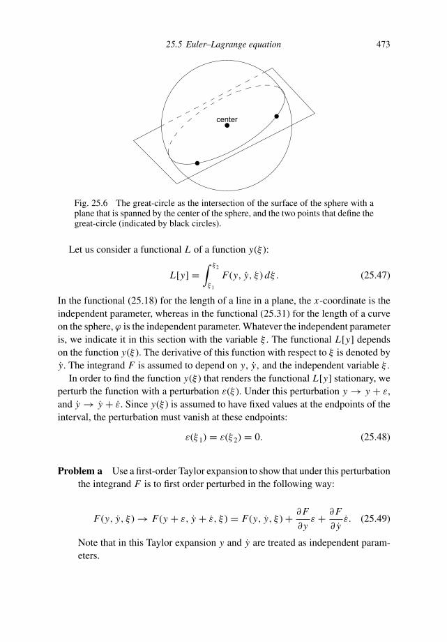
25.5 Euler–Lagrange equation 473
center
Fig. 25.6 The great-circle as the intersection of the surface of the sphere with aplane that is spanned by the center of the sphere, and the two points that define thegreat-circle (indicated by black circles).
Let us consider a functional L of a function y(ξ ):
L[y] =∫ ξ 2
ξ 1
F(y, y, ξ ) dξ . (25.47)
In the functional (25.18) for the length of a line in a plane, the x-coordinate is theindependent parameter, whereas in the functional (25.31) for the length of a curveon the sphere, ϕ is the independent parameter. Whatever the independent parameteris, we indicate it in this section with the variable ξ . The functional L[y] dependson the function y(ξ ). The derivative of this function with respect to ξ is denoted byy. The integrand F is assumed to depend on y, y, and the independent variable ξ .
In order to find the function y(ξ ) that renders the functional L[y] stationary, weperturb the function with a perturbation ε(ξ ). Under this perturbation y → y + ε,and y → y + ε. Since y(ξ ) is assumed to have fixed values at the endpoints of theinterval, the perturbation must vanish at these endpoints:
ε(ξ 1) = ε(ξ 2) = 0. (25.48)
Problem a Use a first-order Taylor expansion to show that under this perturbationthe integrand F is to first order perturbed in the following way:
F(y, y, ξ ) → F(y + ε, y + ε, ξ ) = F(y, y, ξ ) + ∂ F
∂yε + ∂ F
∂ yε. (25.49)
Note that in this Taylor expansion y and y are treated as independent param-eters.
474 Variational calculus
Problem b Insert this relation into expression (25.47) and derive that the first-order perturbation in the functional L is given by
δL =∫ ξ 2
ξ 1
(
∂ F
∂yε + ∂ F
∂ yε
)
dξ . (25.50)
Problem c Carry out an integration by parts of the second term, and show thatwith the boundary conditions (25.48) the first-order perturbation is given by
δL =∫ ξ 2
ξ 1
(
∂ F
∂y− d
dξ
(
∂ F
∂ y
))
ε(ξ ) dξ . (25.51)
This first-order perturbation vanishes for every perturbation ε(ξ ) when
∂ F
∂y− d
dξ
(
∂ F
∂ y
)
= 0. (25.52)
This equation is called the Euler–Lagrange equation; it constitutes a differentialequation for the function y that renders the functional L stationary.
The derivation of the Euler–Lagrange equation is not particularly difficult. How-ever, when using this equation it is important to keep track of the different typesof derivatives. The partial derivatives ∂/∂y and ∂/∂ y treat y and y as independentparameters. This may be confusing because y is the derivative of y with respectto ξ . The notation with partial derivatives is used to denote the dependence of Fon y and y, respectively. The derivative d/dξ is a total derivative. This means thatthe derivative acts on all quantities and the chain law must be used to compute thisderivative.
Let us see how this works for the particular example of the minimization of thelength of the curve in Section 25.3. According to expression (25.18) we have inthat case
F(y, y, x) =√
1 + y2. (25.53)
Since F does not depend explicitly on y, the partial derivative of F with respect to yvanishes: ∂ F/∂y = 0. Furthermore, ∂ F/∂ y = y/
√
1 + y2. Inserting these resultsin the Euler–Lagrange equation and using that x plays the role of the independentvariable ξ gives
0 − d
dx
(
y√
1 + y2
)
= 0. (25.54)
This equation is identical to expression (25.25). The Euler–Lagrange equation thusgives the same result as the treatment of Section 25.3.

25.5 Euler–Lagrange equation 475
As a second example let us consider the determination of the curve with theshortest distance between two points on a sphere. According to expression (25.31),in that case
F(θ, θ , ϕ) =√
θ2 + sin2 θ. (25.55)
In this problem, ϕ plays the role of the independent variable ξ , and the function yis denoted by θ . When encountering a problem with a different notation, it is oftenuseful to reformulate the Euler–Lagrange equation for the variables that are used.In this particular problem the Euler–Lagrange equation (25.52) is given by
∂ F
∂θ− d
dϕ
(
∂ F
∂θ
)
= 0. (25.56)
The partial derivatives with respect to θ and θ are given by
∂ F
∂θ= sin θ cos θ
√
θ2 + sin2 θ
,
∂ F
∂θ= θ
√
θ2 + sin2 θ
.
(25.57)
Inserting these values in the Euler–Lagrange equation (25.56) gives
sin θ cos θ√
θ2 + sin2 θ
− d
dϕ
⎛
⎝
θ√
θ2 + sin2 θ
⎞
⎠ = 0. (25.58)
Problem d Verify that this expression is identical to equation (25.39).
The examples shown here imply that the Euler–Lagrange equation gives the sameresults as we derived in the previous sections. We have covered the simplest casewhere y(ξ ) depends on one variable only and where the endpoints of the functiony are fixed. The treatment can be generalized to include functions y that depend onmore than one independent variable, functions whose endpoints are not necessarilyfixed, and functionals that also contain the second derivative y. Details can be foundin reference [95].
The treatment of this section can be generalized for the situation that the func-tional depends on several different variables. This is for example the case when onewants to minimize a functional that depends on the trajectory r(ξ ) that depends on

476 Variational calculus
three spatial coordinates. In that case, the functional depends on the coordinates r:
F = F[r], (25.59)
where r is a function of the independent parameter ξ . The curve that renders thisfunctional stationary can be found by changing the trajectory r(ξ ) with a vectorperturbation ε(ξ ), and by requiring that to first order in ε(ξ ) the functional doesnot change. This perturbation in general has three components as well. However,nothing keeps us from perturbing one of the components of ε only, let us denotethis component with εi . Let the components of the vector r be denoted by yi . Thederivation in expressions (25.48)–(25.52) can be repeated for that case, with the onlychange that the variable ε must be replaced by εi . This gives the Euler–Lagrangeequation for each of the components yi :
∂ F
∂yi− d
dξ
(
∂ F
∂ yi
)
= 0. (25.60)
25.6 Lagrangian formulation of classical mechanics
In this section we consider a particle with mass m that moves in one dimension. Themass m is not necessarily constant. In order to relate this problem to the notationof the previous section we denote the location of the particle with the coordinatey. The particle starts at a location y1 at time t1 and moves to the endpoint y2 whereit arrives at time t2. The kinetic energy of the particle is given by EK = my2/2,where the dot denotes the time derivative: y ≡ dy/dt . The time t now plays therole of the independent variable ξ . The potential energy of the particle is given byEP = V (y), where V describes the potential in which the particle moves. Let usconsider the difference of the kinetic and potential energy integrated over time:
A[y] ≡∫ t2
t1
(
1
2my2 − V (y)
)
dt, (25.61)
this quantity is called the action [44]. At this moment there is no specific reasonyet to compute the action, but we will see that the trajectory y(t) that renders theaction stationary has a special meaning.
In the notation of equation (25.47) the integrand of the action is given by
L(y, y, t) = 1
2my2 − V (y), (25.62)
this quantity is called the Lagrangian [44].
25.6 Lagrangian formulation of classical mechanics 477
Problem a Verify that the partial derivatives of the Lagrangian with respect to yand y are given by
∂L
∂y= −∂V
∂y,
∂L
∂ y= my.
(25.63)
Problem b Insert these results in the Euler–Lagrange equation to show that thetrajectory y(t) that renders the action stationary is given by
d
dt(my) = −∂V
∂y. (25.64)
The derivative −∂V/∂y is simply the force F that acts on the particle. Since y isthe velocity, my is the momentum, and equation (25.64) is equivalent to Newton’slaw: d(mv)/dt = F . This result gives us a new way to interpret the motion of aparticle in classical mechanics. The Lagrangian (25.62) is the difference of thekinetic and potential energy. This means that in classical mechanics a particlefollows a trajectory such that the time-averaged difference between the kinetic andpotential energy is minimized. This is one example of the variational formulationof classical mechanics. More details and many examples can be found in references[44, 60].
Let us redo this problem in three dimensions. In that case the action is given by
A ≡∫ t2
t1
(
1
2my2 − V (y)
)
dt, (25.65)
where y(t) describes the trajectory of the particle as a function of time.
Problem c Use the Euler–Lagrange equation (25.60) to show that this functionalis stationary when
d
dt(myi ) = −∂V
∂yi. (25.66)
In vector-form this expression can be written as
d
dt(my) = −∇V . (25.67)
This is Newton’s law in three dimensions for a force that is related to the potentialby F = −∇V .
478 Variational calculus
25.7 Rays are curves of stationary travel time
In Section 12.4 we discussed geometric ray theory as a high-frequency approxi-mation to solutions of the wave equation. In this section we develop an alternativeview on ray theory. When a wave travels along a segment of a ray with lengthds, and if the wave velocity is denoted by c, then the time needed to cover thisdistance is given by dt = c−1ds. In this section we use the symbol u for slowness,the reciprocal of velocity:
u ≡ 1/c. (25.68)
Using this definition, the total travel time along the ray is given by
T =∫
u(r) ds. (25.69)
In this section we consider the trajectories that render the travel time stationary.The integral (25.69) suggests use of the arc-length s as independent parameter.
This is, however, not a good idea since it is not known how long the ray thatconnects a source to a receiver will be. For this reason the endpoint condition(25.48) cannot be applied because it is not known what ξ 2 is. The travel timecannot be used as independent parameter either, because it is the travel time thatwe seek to optimize. Instead we will use the relative arc-length as independentparameter. Let the total length of the ray be denoted by S. The relative arc-length isdefined as
ξ ≡ s/S. (25.70)
At the starting point of the ray ξ = 0, while at the endpoint ξ = 1.At this moment we do not know S yet, but this quantity can be related to the
curve r(ξ ) by using that
ds =∣
∣
∣
∣
drdξ
∣
∣
∣
∣
dξ = |r| dξ =√
x2 + y2 + z2 dξ . (25.71)
Problem a Use these results to show that the travel time can be written as
T [r] =∫ 1
0F(r, r) dξ, (25.72)
with
F(r, r) = u(r)√
x2 + y2 + z2. (25.73)

25.7 Rays are curves of stationary travel time 479
Problem b The curve that renders the travel time stationary follows from theEuler–Lagrange equation (25.60). Show that
∂ F
∂x= ∂u
∂x
√
x2 + y2 + z2, (25.74)
and
∂ F
∂ x= u
x√
x2 + y2 + z2. (25.75)
Problem c Use these results to show that the Euler–Lagrange equation (25.60)for the variable x is given by
d
dξ
(
ux
√
x2 + y2 + z2
)
= ∂u
∂x
√
x2 + y2 + z2. (25.76)
Similar equations hold for the variables y and z. In order to interpret this equation,we introduce the unit vector n, whose x-component is defined by
nx ≡ x√
x2 + y2 + z2, (25.77)
with a similar definition for the y- and z-components.
Problem d Show that this vector is of unit length: |n| = 1.
Problem e Expression (25.71) can be used to convert the ξ -derivative in expres-sion (25.76) into a derivative along the curve, by using
d
dξ= ds
dξ
d
ds=
√
x2 + y2 + z2d
ds. (25.78)
Use these results to show that the Euler–Lagrange equation (25.76) can bewritten as
d
ds(unx ) = ∂u
∂x. (25.79)
Similar expressions hold for the y- and z-components of the Euler–Lagrangeequation. In vector-form the Euler–Lagrange equation can be written as
d
ds(un) = ∇u. (25.80)

480 Variational calculus
With definition (25.77), the unit vector n can be rewritten in the following way
n = dr/dξ√
x2 + y2 + z2= dr
dξ
dξ
ds= dr
ds, (25.81)
where expression (25.78) is used in the second identity. Using this result in equation(25.80), and using that u = c−1 gives
d
ds
(
1
c
drds
)
= ∇(
1
c
)
. (25.82)
This equation is called the equation of kinematic ray tracing.The equation of kinematic ray tracing can be derived from the eikonal equation
(12.25) that was derived from the high-frequency approximation to the wave equa-tion [3]. The eikonal equation (12.25) describes the propagation of wave-fronts,while the equation of kinematic ray tracing (25.82) describes the propagation ofrays. These equations are equivalent and provide a complementary view of geomet-ric ray theory. In this section we derived the equation of kinematic ray tracing fromthe requirement that the travel time is stationary. This means that rays are curvesthat render the travel time stationary. Most often, rays are curves that minimizethe travel time. However, seismic waves that reflect once off the Earth’s surfaceare so-called minimax arrivals. The travel time increases when the ray is perturbedin one direction and it decreases when the ray is perturbed in another direction.Whether a ray is a minimum time arrival or a minimax arrival can be detected inthe phase of the arriving waves. Observations of this phenomenon are shown byChoy and Richards [25].
It is interesting to convert the derivative d/ds in expression (25.82) into a timederivative by using that
d
ds= dt
ds
d
dt= 1
c
d
dt. (25.83)
This changes the equation of kinematic ray tracing into
d
dt
(
1
c2
drdt
)
= c∇(
1
c
)
. (25.84)
This expression can be compared with Newton’s law (25.67) for a particle with amass m that may vary with time:
d
dt
(
mdrdt
)
= F. (25.85)
These equations are identical when 1/c2 in (25.84) is equated to the mass m in(25.85), and when c∇ (1/c) takes the role of the force F in Newton’s law. In classicalmechanics it is the force that makes a trajectory curve. Therefore, in geometric ray

25.8 Lagrange multipliers 481
theory it is the velocity gradient that makes a ray curve. The close analogy betweengeometric ray theory and classical mechanics has led to a wide body of theorythat utilizes the same mathematical tools for classical mechanics and geometric raytheory [11, 38].
25.8 Lagrange multipliers
Often in minimization there is a constraint that the solution should satisfy. In Section25.10 we consider the problem of a wire that is suspended between two points. Theshape of the wire is dictated by the requirement that its potential energy in thegravitational field is minimized. Obviously, the potential energy is smallest whenthe wire curves down as much as possible. The constraint that the wire has agiven length restricts the downward displacement of the wire. This amounts to aconstrained optimization problem where the potential energy is minimized underthe constraints that the wire has a fixed length. Problems like this can be solved witha technique called Lagrange multipliers. In this section we introduce this techniquefirst with a finite-dimensional problem, and then generalize it to problems withinfinitely many degrees of freedom.
To fix our mind we consider the following question: what is the point on thesurface of a ball that has the lowest potential energy in a gravitational field? This isa trivial problem, and the solution obviously is given by the point at the bottom ofthe ball. Here we solve this problem while introducing the technique of Lagrangemultipliers.
Let us first cast the condition that the point lies on the surface of the ball in amathematical form. When the ball has a radius R and is centered on the origin, thisconstraint is given by
C(x, y, z) = x2 + y2 + z2 = R2. (25.86)
The constraint thus implies that C(x, y, z) = constant. Suppose that we move apoint r = (x, y, z) along the surface of the ball with an infinitesimal displacementδr, as shown in Figure 25.7. Since the displaced point r + δr must lie on the surfaceof the ball as well, it must satisfy
C(r + δr) = C(r) (25.87)
Problem a Use equation (5.8) to show that this implies that
∇C · δr = 0. (25.88)

482 Variational calculus
rdrd
V
C
C
V
A
B
Fig. 25.7 The direction of the vectors ∇C and ∇V at two points on a ball. Thedashed lines indicate the equipotential surfaces where V = constant.
Geometrically this condition states that δr is perpendicular to the gradient ∇C . Forour particular problem, ∇C points in the radial direction, so the condition (25.87)simply states that the point is perturbed along the surface of the sphere.
We want to minimize the potential energy V (r) associated with the gravitationalfield as a function of the location r. Under a perturbation δr, the potential energyis to first order changed by an amount
δV = (∇V · δr). (25.89)
The potential energy is minimized when this quantity vanishes, this is the case whenthe displacement δr is perpendicular to ∇V .
How can we see that the point A in the sphere in Figure 25.7 does not minimizethe potential energy, but that the point B does minimize the potential energy? Con-sider the displacement δr at point A along the surface of the sphere. At point A thedisplacement δr is not perpendicular to the gradient ∇V . According to expression(25.89) this implies that the potential energy changes to first order under this per-turbation, hence point A does not minimize the potential energy. At point B, thedisplacement δr is perpendicular to the vector ∇V , so that at that point the potentialenergy does not change to first order under this perturbation. In other words, pointB is an extremum of the potential energy.
At point A the vectors ∇C and ∇V are not parallel; the vector ∇C points in theradial direction while the vector ∇V points downward. However, at the minimumof the potential energy at point B, these vectors are parallel, see Figure 25.7. This

25.8 Lagrange multipliers 483
means that at the minimum the gradient vectors satisfy
∇C = −λ∇V . (25.90)
The constant −λ accounts for the fact that the vectors in general have a differentlength. The minus sign is introduced in order to conform to the notation most oftenfound in the literature; it has no specific meaning. The constant λ is called theLagrange multiplier. Equation (25.90) can also be written as
∇ (V + λC) = 0. (25.91)
For the unconstrained minimization of the potential energy, we just needed to solvethe equation ∇V = 0. The constraint that the point lies on the surface of the ballleads to the minimization problem (25.91). Note that this problem contains theunknown parameter λ, hence the constrained minimization problem depends onthe four variables x , y, z, and λ, whereas the original problem was dependent onlyon the three variables x , y, and z. However, the constrained minimization problemhas an extra equation that should be satisfied: the constraint (25.86). This meansthat we now have four equations with four unknowns.
Yet another way to see that point B minimizes the potential energy is the fol-lowing. The constraint states that the point lies on the surface of the sphere. Stateddifferently, the point must lie on the surface C(x, y, z) = constant. At the extremumof the potential energy, this surface must touch the surface V (x, y, z) = constant;if it would intersect that surface at an angle the point could be moved along thesurface C(x, y, z) = constant while raising or lowering the potential energy. Thiscontradicts the fact that the point maximizes or minimizes the potential energy.This means the extremum of the potential energy is attained at the points wherethe surfaces C(x, y, z) = constant and V (x, y, z) = constant are tangent. (When aball lies on the ground, the surface of the ball and the ground touch each other.) Adifferent way of stating this is that the vectors ∇C and ∇V are parallel, which isequivalent to condition (25.90).
Let us see how the machinery of the Lagrange multipliers works for finding thepoint on a ball that has the lowest potential energy. In this case the potential energyis given by
V (r) = z, (25.92)
and the constraint that the point lies on a sphere with radius R is given by (25.86).For this example, V + λC = z + λ(x2 + y2 + z2).
484 Variational calculus
Problem b Show that for this problem equation (25.91) leads to⎛
⎝
2λx2λy
1 + 2λz
⎞
⎠ = 0. (25.93)
This expression constitutes three equations for the four unknowns x , y, z, and λ.The first two lines dictate that x = y = 0. The last line states that z = −1/2λ.
Problem c Use the constraint (25.86) to show that λ = ±1/2R.
This means that the solution is given by
r =⎛
⎝
00
±R
⎞
⎠ . (25.94)
The potential energy has extrema for the top and the bottom of the sphere. The topof the sphere maximizes the potential energy, while at the bottom of the sphere thepotential energy has a minimum.
In the treatment of this section, it is not essential that the constraint C(r) describesthe surface of the sphere, and the V (r) is the potential energy. The employed argu-ments hold for the minimization of any function V (r) under a constraint C(r). Aslong as the gradient of these functions is well-defined the constrained optimizationproblem can be solved with expression (25.91).
The extension of Lagrange multipliers to the constrained optimization of func-tionals is not trivial. Here we sketch the main idea. Suppose we want to minimizethe functional
L[y] =∫
F(y, y, ξ ) dξ, (25.95)
subject to the constraint∫
C(y, y, ξ )dξ = constant. (25.96)
Suppose that y(ξ ) is modified with a perturbation ε(ξ ) such that the perturbedfunction also satisfies the constraint (25.96). This means that the perturbation ofthe constraint is given by
∫ (
∂C
∂yε + ∂C
∂ yε
)
dξ = 0. (25.97)
Using an integration by parts, as in Section 25.5, then gives∫ (
∂C
∂y− d
dξ
(
∂C
∂ y
))
ε(ξ ) dξ = 0. (25.98)
25.9 Designing a can with an optimal shape 485
This equation is equivalent to expression (25.87) for a finite-dimensional problem.With a similar argument, the minimization of the functional (25.95) leads to thecondition
∫ (
∂ F
∂y− d
dξ
(
∂ F
∂ y
))
ε(ξ ) dξ = 0. (25.99)
The last two expressions state that the functions
(
∂C/∂y − d
dξ(∂C/∂ y)
)
and(
∂ F/∂y − d
dξ(∂ F/∂ y)
)
are both “perpendicular” to the perturbation ε(ξ ), just
like ∇C and ∇V were perpendicular to the perturbation δr of the point on the sphere.Since this must hold for any perturbation ε(ξ ), this means that these functions are“parallel” to each other:
(
∂ F
∂y− d
dξ
(
∂ F
∂ y
))
= −λ
(
∂C
∂y− d
dξ
(
∂C
∂ y
))
. (25.100)
The is the analogue of equation (25.90). This argument is not rigorous, the quo-tation marks highlight a vague use of the concepts perpendicular and parallel. Amore thorough (and more complex) derivation is given by Smith [95]. However,accepting expression (25.100), the constrained optimization problem is given by theequation
∂ (F + λC)
∂y− d
dξ
(
∂ (F + λC)
∂ y
)
= 0. (25.101)
This expression is nothing but the Euler–Lagrange equation for the function F +λC . The constrained optimization problem can thus be solved by optimizing F +λC . This introduces the additional parameter λ. This parameter can be found bysolving the constraint (25.96).
25.9 Designing a can with an optimal shape
In this section we return to the problem of Sections 25.1 and 25.2 where we treatedthe design of the shape of a can that maximizes the content for a given surfacearea. We treat this problem here using the Lagrange multiplier. Let us consider thedesign problem in a slightly different way by assuming that the surface area S ofthe bottom and the top of the can is fixed. We noted in Section 25.2 that the volumeof the can is largest when the circumference C is minimized for a fixed value of thesurface S of the top and bottom.
486 Variational calculus
The circumference is related to the radius r (ϕ) by expression (25.14). The surfacearea of the top and bottom is given by
S = 1
2
∫ 2π
0r2dϕ. (25.102)
According to the theory of the previous section, this constrained optimization prob-lem can be solved by optimizing C + λS, where the Lagrange multiplier λ followsfrom the constraint (25.102).
Problem a Use expressions (25.14) and (25.102) to show that the constrainedoptimization problem is solved by solving the Euler–Lagrange equation for
F(r, r ) =√
r2 + r2 + λ
2r2. (25.103)
Problem b Show that
∂ F
∂r= r√
r2 + r2+ λr, (25.104)
and
∂ F
∂ r= r√
r2 + r2. (25.105)
Problem c Take the total derivative of the previous expression with respect to ϕ
and show that the Euler–Lagrange equation for this optimization problem isgiven by
rr2 − r2r(
r2 + r2)3/2 = r√
r2 + r2+ λr. (25.106)
Problem d This is a nonlinear differential equation. However, we know fromSection 25.2 that a constant radius is likely to be a solution. Show that thesolution r (ϕ) = constant reduces equation (25.106) to
1 + λr = 0. (25.107)
Problem e This condition implies that r = −λ−1. Determine the Lagrange mul-tiplier λ by inserting this expression into the constraint (25.102) to show that
λ =√
π/S, (25.108)
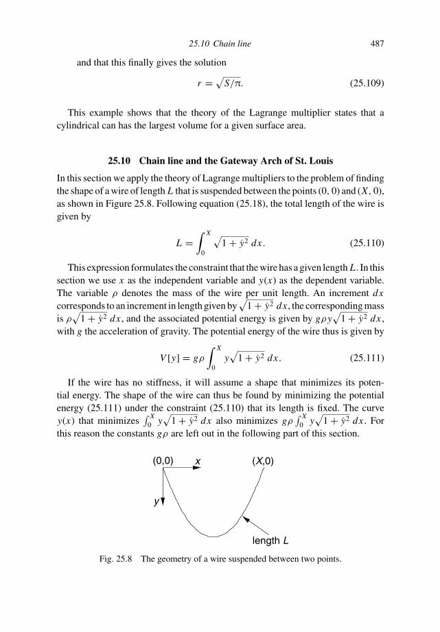
25.10 Chain line 487
and that this finally gives the solution
r =√
S/π. (25.109)
This example shows that the theory of the Lagrange multiplier states that acylindrical can has the largest volume for a given surface area.
25.10 Chain line and the Gateway Arch of St. Louis
In this section we apply the theory of Lagrange multipliers to the problem of findingthe shape of a wire of length L that is suspended between the points (0, 0) and (X, 0),as shown in Figure 25.8. Following equation (25.18), the total length of the wire isgiven by
L =∫ X
0
√
1 + y2 dx . (25.110)
This expression formulates the constraint that the wire has a given length L . In thissection we use x as the independent variable and y(x) as the dependent variable.The variable ρ denotes the mass of the wire per unit length. An increment dxcorresponds to an increment in length given by
√
1 + y2 dx , the corresponding massis ρ
√
1 + y2 dx , and the associated potential energy is given by gρy√
1 + y2 dx ,with g the acceleration of gravity. The potential energy of the wire thus is given by
V [y] = gρ
∫ X
0y√
1 + y2 dx . (25.111)
If the wire has no stiffness, it will assume a shape that minimizes its poten-tial energy. The shape of the wire can thus be found by minimizing the potentialenergy (25.111) under the constraint (25.110) that its length is fixed. The curvey(x) that minimizes
∫ X0 y
√
1 + y2 dx also minimizes gρ∫ X
0 y√
1 + y2 dx . Forthis reason the constants gρ are left out in the following part of this section.
(0,0) (X,0)x
y
length L
Fig. 25.8 The geometry of a wire suspended between two points.

488 Variational calculus
According to the discussion of Section 25.8 the solution of this constrained opti-mization problem can be found by optimizing V + λL , and by using the constraint(25.110) to find the Lagrange multiplier λ.
Problem a Use the theory of the previous section to show that the shape of thewire is found by optimizing
F[y] =∫ X
0F(y, y) dx, (25.112)
with
F(y, y) = y√
1 + y2 + λ√
1 + y2 (25.113)
Problem b Show that
∂F∂y
=√
1 + y2, (25.114)
and
∂F∂ y
= y√
1 + y2(y + λ). (25.115)
Problem c Take the total derivative of the last expression to derive that
d
dx
(
∂F∂ y
)
= 1(
1 + y2)3/2
y(y + λ) + y2√
1 + y2
. (25.116)
Remember that in this derivative all variables that depend on x are differenti-ated.
Problem d Show that the Euler–Lagrange equation for this problem can be writ-ten as
1 + y2 = y(y + λ). (25.117)
This is a non-linear differential equation that displays the complexity that oftenresults in the solution of variational problems. There is no simple way to guess thesolution, or to construct it in a systematic way. For this reason we simply state thefollowing trial solution
y(x) = A cosh (B(x + h)) + C, (25.118)
where A, B, C , and h are constants.

25.10 Chain line 489
Problem e Insert this solution into the differential equation (25.117) and showthat the result can be written as
(1 − A2 B2) = AB2(λ + C) cosh (B(x + h)) . (25.119)
The left-hand side of this expression is independent of x , while the right-hand sidevaries with x . This is possible only when the coefficients of the left-hand side andthe right-hand side vanish. This implies that
1 − A2 B2 = 0 and AB2(λ + C) = 0. (25.120)
These equations are satisfied when A = 1/B and C = −λ, so that the solution isgiven by
y(x) = 1
Bcosh (B(x + h)) − λ. (25.121)
This expression contains three constants. There are, however, three pieces of in-formation that we have not used yet: the boundary conditions which state the wiregoes through the points (0, 0) and (X, 0), and the constraint (25.110) which statesthat the wire has length L .
Problem f Use the boundary conditions to show that h = −X/2 and λ =B−1 cosh (X/2), so that the solution is given by
y(x) = B−1
cosh
(
B
(
x − X
2
))
− cosh
(
B X
2
)
. (25.122)
Problem g Insert this solution into the constraint (25.110) and show that thisleads to the following equation for the constant B:
2
Bsinh
(
B X
2
)
= L (25.123)
This is a transcendental equation that cannot be solved in closed form, but it canbe solved numerically. This completes the solution of finding the shape of a wiresuspended between two points.
It follows from equation (25.122) that the wire is shaped like the cosine-hyperbolic. This curve is called the catenary; this word is derived from the Latinword catena that means chain. The catenary can be seen in the chain that is sus-pended in the background of Figure 25.9. Knowing the shape of a suspended wireis more than a mathematical curiosity. A suspended wire has in general such a

490 Variational calculus
Fig. 25.9 The chain in the background, and the arch in the foreground have theshape of a catenary. The arch consists of blocks of foam that are not glued together.The figure is made by high-school students and is reproduced with permission ofthe New Trier Connections Project.
tension
tension
gravity
gravity
compression
com
pres
sion
Fig. 25.10 The balance of the tensional forces and gravity for a suspended wire(left panel), and the balance between tensional forces and the gravitational forcefor an arch (right panel).
small stiffness that this property can be ignored. (In the analysis of this section thewire does not have any stiffness.) This means that the wire does not support anyinternal bending moments. The shape of the wire is dictated by the balance of thegravitational force and the net tensional force that arises from the curvature of thewire as shown in the left panel of Figure 25.10.
Let us suppose we turn the wire upside down and that we build an arch. Inthat case the gravitational force acts into the arch and the tensional forces of theleft panel of Figure 25.10 are changed into compressional forces that balances thegravitational force, as shown in the right panel of Figure 25.10. This implies that an
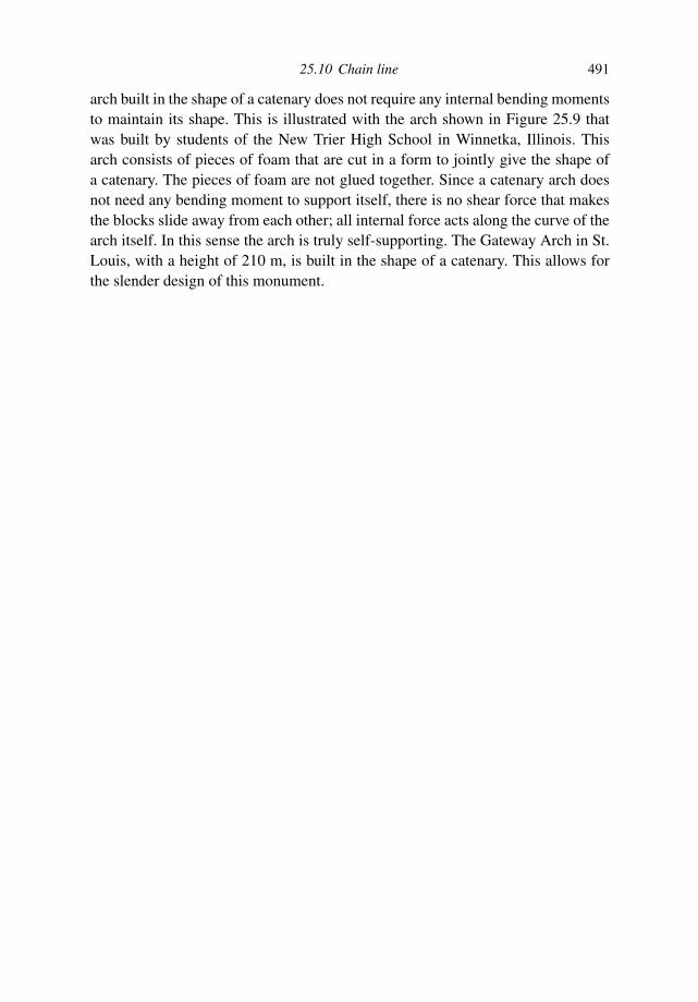
25.10 Chain line 491
arch built in the shape of a catenary does not require any internal bending momentsto maintain its shape. This is illustrated with the arch shown in Figure 25.9 thatwas built by students of the New Trier High School in Winnetka, Illinois. Thisarch consists of pieces of foam that are cut in a form to jointly give the shape ofa catenary. The pieces of foam are not glued together. Since a catenary arch doesnot need any bending moment to support itself, there is no shear force that makesthe blocks slide away from each other; all internal force acts along the curve of thearch itself. In this sense the arch is truly self-supporting. The Gateway Arch in St.Louis, with a height of 210 m, is built in the shape of a catenary. This allows forthe slender design of this monument.

26
Epilogue, on power and knowledge
We all continue to feel a frustration because of our inability to foresee the soul’sultimate fate. Although we do not speak about it, we all know that the objec-tives of our science are, from a general point of view, much more modest thanthe objectives of, say, the Greek sciences were; that our science is more suc-cessful in giving us power than in giving us knowledge of truly human interest.[E. P. Wigner, 1972, The place of consciousness in modern physics, in Conscious-ness and Reality, eds. C. Muses and A. M. Young, New York, Outerbridge andLizard, pp. 132–141].
In this book we have explored many methods of mathematics as used in thephysical sciences.Mathematics plays a central role in the physical sciences becauseit is the only language we have for expressing quantitative relations in the worldaround us. In fact, mathematics not only allows us to express phenomena in aquantitative way, it also has a remarkable predictive power in the sense that it allowsus to deduce the consequences of natural laws in terms of measurable quantities. Infact, we do not quite understandwhymathematics gives such an accurate descriptionof the world around us [120].
It is truly stunning how accurate some of the predictions in (mathematical)physics have been. The orbits of the planetary bodies can now be computed withan extreme accuracy. Morrison and Stephenson [72] compared the path of a solareclipse at 181 BC with historic descriptions made in a city in eastern China thatwas located in the path of the solar eclipse. According to the computations, the pathof the solar eclipse passed 50 degrees west of the site of this historic observation.This eclipse took place about 2000 years ago; this means that the Earth has rotatedthrough about 2.8 × 10⁸ degrees since the eclipse. The relative error in the pathof the eclipse over the Earth is thus only 1.7 × 10⁻⁷. In fact, this discrepancy of50 degrees can be explained well by the observed deceleration of the Earth [72]due to the braking effect of the Earth’s tides.
492
Epilogue, on power and knowledge 493
The light emitted by hydrogen atoms has discrete spectral lines which are due tothe fact that electrons behave as standingwaves.Every electron is coupled to thefieldof electromagnetic radiation (light). There is a small chance that an electron willemit and re-absorb a virtual photon [91]. (Photons are the light-quanta.) This leads tothe so-called Lamb shift of the spectral lines of light radiated by excited hydrogenatoms. For hydrogen atoms the shift for the transition between the 2s and 2p1/2state is 1060 MHz. This corresponds to a reciprocal wavelength of 0.035 cm−1,the reciprocal wavelength that corresponds to the ionization energy is 2700 cm−1.Compared to the ionization energy of the ground state this corresponds thereforeto a relative frequency shift of 1.3 × 10⁻⁶. This is in very good agreement withobservations. It is interesting to note that this prediction of the Lamb shift is basedon second order perturbation theory [91]. This means that an approximate theoryprovides a stunningly accurate prediction of the Lamb shift.
A third example of the extreme accuracy of mathematics in the physical sciencesis the perihelion precession of Mercury [76]. According to the laws of Newton, aplanet will orbit in a fixed ellipsoidal orbit around the Sun. The general theory ofrelativity predicts that this ellipse slowly changes its position; the point of the ellipseclosest to the Sun (the perihelion) slowly precesses around the Sun. According tothe theory of general relativity this precession is given by 42.98 arcsec/century,whereas the observed precession rate is 43.1 ± 0.1 arcsec/century. Note that thisprecession rate is extremely small, but that it is well predicted from theory.
Mathematics not only provides us with valuable and stunningly accurate in-sights in the world around us, it is also an indispensable tool in making technicalinnovations. The design and implementation of rockets, aircraft, chemical plants,water treatment systems, modern electronics, information technology, and manyother innovations would have been impossible without mathematics. Mathematicsand the physical sciences have created many new opportunities for mankind. Forthis reason one can state that mathematics and the physical sciences have greatlyincreased our power to modify the world in which we live; see also the quote ofNobel prize laureate Wigner [121] at the beginning of this section.
The problem with releasing power is that it can be used for good and for badpurposes. Science is objective in the sense that a certain theory is either consistentwith observations, or it is not. However, scientific knowledge does not come withthemoral standard that tells us how the power that we release in our scientific effortsshould be used. It is essential that each of us develops such a standard, so that thefruits of our knowledge can be used for the benefit of mankind and the world weinhabit.

References
[1] Abramowitz, M. and I. A. Stegun, 1965, Handbook of Mathematical Functions,New York, Dover Publications.
[2] Aharonov, Y., and D. Bohm, 1959, Significance of electromagentic potentials inthe quantum theory, Phys. Rev., 115, 485–491.
[3] Aki, K. and P. G. Richards, 2002, Quantitative Seismology, 2nd edition, Sausalito,University Science Books.
[4] Aldridge, D. F., 1994, Linearization of the eikonal equation, Geophysics, 59,1631–1632.
[5] Arfken, G. B., 1995, Mathematical Methods for Physicists, San Diego, AcademicPress.
[6] Ashby, N., 2002, Relativity and the Global Positioning System, Phys. Today,55(5), 41–47.
[7] Backus, M.M., 1959, Water reverberations – their nature and elimination,Geophysics, 24, 233–261.
[8] Barish, B. C. and R. Weiss, 1999, LIGO and the detection of gravitational waves,Phys. Today, 52(10), 44–55.
[9] Barton, G., 1989, Elements of Green’s Functions and Propagation, Potentials,Diffusion and Waves, Oxford, Oxford Scientific Publications.
[10] Beissner, K., 1998, The acoustic radiation force in lossless fluids in Eulerian andLagrangian coordinates, J. Acoust. Soc. Am., 103, 2321–2332.
[11] Bennett, J. A., 1973, Variations of the ray path and phase path: a Hamiltonianformulation, Radio Sci., 8, 737–744.
[12] Bevington P. R. and D.K. Robinson, 1992, Data reduction and Error Analysis forthe Physical Sciences, New York, McGraw-Hill.
[13] Bellman, R. and R. Kalaba, 1960, Invariant embedding and mathematical physicsI. Particle processes, J. Math. Phys., 1, 280–308.
[14] Bender, C.M. and S. A. Orszag, 1978, Advanced mathematical Methods forScientists and Engineers, New York, McGraw-Hill.
[15] Berry, M.V. and S. Klein, 1997, Transparent mirrors: rays, waves and localization,Eur. J. Phys., 18, 222–228.
[16] Berry, M.V. and C. Upstill, 1980, Catastrophe optics: Morphologies of causticsand their diffraction patterns, Prog. Optics, 18, 257–346.
[17] Blakeley, R. J., 1995, Potential Theory in Gravity and Magnetics, Cambridge,Cambridge University Press.
494

References 495
[18] Bleistein, N. and R.A. Handelsman, 1975, Asymptotic Expansions of Integrals,New York, Dover.
[19] Boas, M. L., 1983, Mathematical Methods in the Physical Sciences, 2nd edition,New York, Wiley.
[20] Brack, M. and R.K. Bhaduri, 1997, Semiclassical Physics, Reading MA,Addison-Wesley.
[21] Brillouin, L., 1960, Wave Propagation and Group Velocity, New York, AcademicPress.
[22] Broglie, L. de, 1952, La Theorie des particules de spin 1/2, Paris, Gauthier-Villars.[23] Buckingham, E., 1914, On physically similar systems; illustrations of the use of
dimensional equations, Phys. Rev., 4, 345–376.[24] Butkov, E., 1968, Mathematical Physics, Reading MA, Addison Wesley.[25] Choy, G. L., and P. G. Richards, 1975, Pulse distortion and Hilbert transformation
in multiply reflected and refracted body waves, Bull. Seismol. Soc. Am., 65, 55–70.[26] Cipra, B., 2000, Misteaks . . . and how to Find Them Before the Teacher Does, 3rd
Edition, Natck MA, A.K. Peters.[27] Claerbout, J. F., 1976, Fundamentals of Geophysical Data Processing, New York,
McGraw-Hill.[28] Claerbout, J. F., 1985, Imaging the Earth’s Interior, Oxford, Blackwell.[29] Chopelas, A., 1996, Thermal expansivity of lower mantle phases MgO and
MgSiO3 perovskite at high pressure derived from vibrational spectroscopy, Phys.Earth. Plan. Int., 98, 3–15.
[30] Coveney, P., and R. Highfield, 1991, The Arrow of Time, London, Harper Collins.[31] Dahlen, F. A., 1979, The spectra of unresolved split normal mode multiples,
Geophys. J. R. Astron. Soc., 58, 1–33.[32] Dahlen, F. A. and I. H. Henson, 1985, Asymptotic normal modes of a laterally
heterogeneous Earth, J. Geophys. Res., 90, 12653–12681.[33] Dahlen, F. A., and J. Tromp, 1988, Theoretical Global Seismology, Princeton,
Princeton University Press.[34] DeSanto, J. A., 1992. Scalar Wave Theory; Green’s Functions and Applications,
Berlin, Springer Verlag.[35] Dziewonski, A.M., and J. H. Woodhouse, 1983, Studies of the seismic source
using normal-mode theory, in Earthquakes: Observations, Theory andInterpretation, edited by H. Kanamori and E. Boschi, Amsterdam, North Holland,pp. 45–137.
[36] Earnshaw, S., 1842, On the nature of molecular forces which regulate theconstitution of the luminiferous ether, Trans. Camb. Phil. Soc., 7, 97–112.
[37] Edmonds, A. R., 1974, Angular Momentum in Quantum Mechanics, 3rd edition,Princeton, Princeton University Press.
[38] Farra, V. and R. Madariaga, 1987, Seismic waveform modeling in heterogeneousmedia by ray perturbation theory, J. Geophys. Res., 92, 2697–2712.
[39] Feynman, R. P., 1975, The Character of Physical Law, Cambridge (MA), MITPress.
[40] Feynman, R. P. and A. R. Hibbs, 1965, Quantum Mechanics and Path Integrals,New York, McGraw-Hill.
[41] Fishbach, E. and C. Talmadge, 1992, Six years of the fifth force, Nature, 356,207–214.
[42] Fletcher, C., 1996, The Complete Walker III, New York, Alfred A. Knopf.[43] Fokkema, J. T. and P.M. van den Berg, 1993, Seismic Applications of Acoustic
Reciprocity, Amsterdam, Elsevier.

496 References
[44] Goldstein, H., 1980, Classical Mechanics, 2nd edition, Reading MA,Addison-Wesley.
[45] Gradshteyn, I. S. and I.M. Rhyzik, 1965, Tables of Integrals, Series and Products,New York, Academic Press.
[46] Gubbins, D. and R. Snieder, 1991, Dispersion of P waves in subducted lithosphere:Evidence for an eclogite layer, J. Geophys. Res., 96, 6321–6333.
[47] Guglielmi, A. V. and O.A. Pokhotelov, 1996, Geoelectromagnetic Waves, Bristol,Inst. of Physics Publ.
[48] Halbwachs, F., 1960, Theorie relativiste des fluides a spin, Paris, Gauthier-Villars.[49] Hildebrand, A. R., M. Pilkington, M. Conners, C. Ortiz-Aleman and R. E. Chavez,
1995, Size and structure of the Chicxulub crater revealed by horizontal gravity andcenotes, Nature, 376, 415–417.
[50] Holton, J. R., 1992, An Introduction to Dynamic Meteorology, San Diego,Academic Press.
[51] Iyer, H.M. and K. Hirahara (eds.), 1993, Seismic Tomography, Theory andPractice, London, Prentice Hall.
[52] Ishimaru, A., 1997, Wave propagation and Scattering in Random Media, Oxford,Oxford University Press.
[53] Jackson, J. D., 1975, Classical Electrodynamics, New York, Wiley.[54] Jeffreys, H., 1924, On certain approximate solutions of linear differential
equations of second order, Phil. London Math. Soc., 23, 428–436.[55] Kermode, A. C., 1996, Mechanics of Flight, 10th edition, Singapore, Longman.[56] Kline, S. J., 1965, Similitude and Approximation Theory, New York, McGraw-Hill.[57] Kravtsov, Yu. A., 1988, Ray and caustics as physical objects, Prog. Optics, 26,
228–348.[58] Kulkarny, V.A., and B. S. White, 1982, Focusing of waves in turbulent
inhomogeneous media, Phys. Fluids, 25, 1770–1784.[59] Lambeck, K., 1988, Geophysical Geodesy, Oxford, Oxford University Press.[60] Lanczos, C., 1970, The Variational Principles of Mechanics, New York, Dover.[61] Lauterborn, W., T. Kurz and M. Wiesenfeldt, 1993, Coherent Optics, Berlin,
Springer Verlag.[62] Lavenda, B. H., 1991, Statistical Physics, a Probabilistic Approach, New York,
John Wiley.[63] Lin, C. C., L. A. Segel and G.H. Handelman, 1974, Mathematics Applied to
Deterministic Problems in the Natural Sciences, New York, Macmillan.[64] Lister, G. S., and P. F. Williams, 1983, The partitioning of deformation in flowing
rock masses, Tectonophysics, 92, 1–33.[65] Love, S. G., and D. E. Brownlee, 1993, A direct measurement of the terrestrial
mass accretion rate of cosmic dust, Science, 262, 550–553.[66] Madelung, E., 1926, Quantentheorie in hydrodynamischer form, Z. Phys., 40, 322.[67] Marchaj, C. A., 1993, Aerohydrodynamics of Sailing, 2nd edition, London, Adlard
Coles Nautical.[68] Marsden, J. E. and A. J. Tromba, 1988, Vector Calculus, New York, Freeman and
Company.[69] Merzbacher, E., 1970, Quantum Mechanics, New York, Wiley.[70] Moler, C. and C. van Loan, 1978, Nineteen dubious ways to compute the
exponential of a matrix, SIAM Review, 20, 801–836.[71] Morley, T., 1985, A simple proof that the world is three dimensional, SIAM
Review, 27, 69–71.[72] Morrison, L. and R. Stephenson, 1988, The sands of time and the Earth’s rotation,
Astronomy and Geophysics, 39(5), 8–13.

References 497
[73] Muirhead, H., 1973, The Special Theory of Relativity, London, Macmillan.[74] Nayfeh, A.H., 1981, Introduction to Perturbation Techniques, New York,
Wiley.[75] Nolet G. (ed.), 1987, Seismic Tomography, with Applications in Global Seismology
and Exploration Geophysics, Dordrecht, Kluwer.[76] Ohanian, H. C. and R. Ruffini, 1994, Gravitation and Spacetime, New York,
Norton.[77] Olson, P., 1989, Mantle convection and plumes, in The Encyclopedia of Solid
Earth Geophysics, ed. D. E. James, New York, Van Nostrand Reinholt.[78] Oort, A. H. and J. P. Peixoto, 1992, Physics of Climate, New York, Springer Verlag.[79] Parker, R. L., 1994, Geophysical Inverse Theory, Princeton NJ, Princeton
University Press.[80] Parker, R. L. and M.A. Zumberge, 1989, An analysis of geophysical experiments
to test Newton’s law of gravity, Nature, 342, 29–31.[81] Parsons, B. and J. G. Sclater, 1977, An analysis of the variation of the ocean floor
bathymetry and heat flow with age, J. Geophys. Res., 32, 803–827.[82] Pedlosky, J., 1979, Geophysical Fluid Dynamics, Berlin, Springer Verlag.[83] Popper, K., 1956, The arrow of time, Nature, 177, 538.[84] Press, W.H., B. P. Flannery, S. A. Teukolsky and W. T. Vetterling, 1986, Numerical
Recipes, Cambridge, Cambridge University Press.[85] Price, H., 1996, Time’s Arrow and Archimedes’ Point, New Directions for the
Physics of Time, New York, Oxford University Press.[86] Rayleigh, Lord, 1917, On the reflection of light from a regularly stratified medium,
Proc. Roy. Soc. Lon., A93, 565–577.[87] Riley, K. F., M. P. Hobson, and S. J. Bence, 1998, Mathematical Methods for
Physics and Engineering, Cambridge, Cambridge University Press.[88] Rossing, T. D., 1990, The Science of Sound, Reading (MA), Addison Wesley.[89] Rummel, R., 1986, Satellite gradiometry, in Mathematical Techniques for
High-resolution Mapping of the Gravitational Field, Lecture notes in the EarthSciences, vol. 7, ed. H. Suenkel, Berlin, Springer Verlag.
[90] Robinson, E. A. and S. Treitel, 1980, Geophysical Signal Analysis, EnglewoodCliffs (NJ), Prentice Hall.
[91] Sakurai, J. J., 1978, Advanced Quantum Mechanics, Reading (MA), AddisonWesley.
[92] Scales, J. A. and R. Snieder, 1997, Humility and nonlinearity, Geophysics, 62,1355–1358.
[93] Schneider, W.A., 1978, Integral formulation for migration in two and threedimensions, Geophysics, 43, 49–76.
[94] Silverman, M. P., 1993, And Yet It Moves; Strange Systems and Subtle Questions inPhysics. Cambridge, Cambridge University Press.
[95] Smith, D. R., 1974, Variational Methods in Optimization, Englewood Cliffs,Prentice-Hall.
[96] Snieder, R. K., 1985, The origin of the 100,000 year cycle in a simple ice agemodel, J. Geophys. Res., 90, 5661–5664.
[97] Snieder, R., 1986, 3D Linearized scattering of surface waves and a formalism forsurface wave holography, Geophys. J. R. astr. Soc., 84, 581–605.
[98] Snieder, R., 1996, Surface wave inversions on a regional scale, in SeismicModelling of Earth Structure, eds. E. Boschi, G. Ekstrom and A. Morelli, Bologna,Editrice Compositori, pp. 149–181.
[99] Snieder, R. and D. F. Aldridge, 1995, Perturbation theory for travel times, J.Acoust. Soc. Am., 98, 1565–1569.

498 References
[100] Snieder, R., 2002, Time-reversal invariance and the relation between wave chaosand classical chaos, in Imaging of Complex Media with Acoustic and SeismicWaves, pp. 1–15, eds. M. Fink, W.A. Kuperman, J. P. Montagner, and A. Tourin,Berlin, Springer Verlag.
[101] Snieder, R. and G. Nolet, 1987, Linearized scattering of surface waves on aspherical Earth, J. Geophys., 61, 55–63.
[102] Spetzler, J. and R. Snieder, 2001, The formation of caustics in two and threedimensional media, Geophys. J. Int., 144, 175–182.
[103] Stacey, F. D., 1992, Physics of the Earth, 3rd edition, Brisbane, Brookfield Press.[104] Tabor, M., 1989, Chaos and Integrability in Nonlinear Dynamics, New York, John
Wiley.[105] Taylor, E. F., and J. A. Wheeler, 1966, Spacetime Physics, San Francisco, Freeman.[106] Tennekes, H., 1997, The Simple Science of Flight: from Insects to Jumbo Jets,
Cambridge MA, MIT Press.[107] Thompson, P. A., 1972, Compressible-fluid Dynamics, New York, McGraw-Hill.[108] Tritton, D. J., 1982, Physical Fluid Dynamics, Wokingham (UK), Van Nostrand
Reinhold.[109] Tromp, J. and R. Snieder, 1989, The reflection and transmission of plane P- and
S-waves by a continuously stratified band: a new approach using invariantembedding, Geophys. J., 96, 447–456.
[110] Turcotte, D. L. and G. Schubert, 2002, Geodynamics, 2nd edition, Cambridge UK,Cambridge University Press.
[111] van Dyke, M., 1978, Perturbation Methods in Fluid Mechanics, Stanford CA,Parabolic Press.
[112] Virieux, J., 1996, Seismic ray tracing, in Seismic Modelling of Earth Structure,eds. E. Boschi, G. Ekstrom and A. Morelli, Bologna, Editrice Compositori,pp. 221–304.
[113] Vogel, S., Exposing life’s limits with dimensionless numbers, Physics Today,51(11), 22–27.
[114] Udias, A., 1999, Principles of Seismology, Cambridge, Cambridge UniversityPress.
[115] Watson, T. H., 1982, A real frequency, wave-number analysis of leaking modes,Bull. Seismol. Soc. Am., 62, 369–394.
[116] Webster, G.M. (ed.), 1981, Deconvolution, Geophysics reprint series, vol. 1, Tulsa,Society of Exploration Geophysicists.
[117] Weisskopf, V. F., 1939, On the self-energy and the electric field of the electron,Phys. Rev., 56, 72–85.
[118] Whitaker, S., 1968, Introduction to Fluid Mechanics, Englewood Cliffs,Prentice-Hall.
[119] Whitham, G. B., 1974, Linear and Nonlinear Waves, New York, Wiley.[120] Wigner, E. P., 1960, The unreasonable effectiveness of mathematics in the natural
sciences, Comm. Pure Appl. Math., 13, 222–236.[121] Wigner, E. P, 1972, The place of consciousness in modern physics, in
Consciousness and reality, eds. C. Muses and A.M. Young, New York,Outerbridge and Lizard, pp. 132–141.
[122] Wu, R. S. and K. Aki, 1985, Scattering characteristics of elastic waves by anelastic heterogeneity, Geophysics, 50, 582–595.
[123] Yilmaz, O., 1987, Seismic Data Processing, Investigations in Geophysics, vol. 2,Tulsa, Society of Exploration Geophysicists.
References 499
[124] Yoder, C. F., J. G. Williams, J. O. Dickey, B. E. Schutz, R. J. Eanes and B.D. Tapley,1983, Secular variation of the Earth’s gravitational harmonic J2 coefficient fromLAGEOS and nontidal acceleration of the Earth rotation, Nature, 303, 757–762.
[125] Zee, A., 2003, Quantum Field Theory in a Nutshell, Princeton NJ, PrincetonUniversity Press.
[126] Ziolkowski, A., 1991, Why don’t we measure seismic signatures? Geophysics, 56,190–201.
[127] Zumberge, M.A., J. R. Ridgway and J. A. Hildebrand, 1997, A towed marinegravity meter for near-bottom surveys, Geophysics, 62, 1386–1393.

Index
acceleration in spherical coordinates37–40
accretion 22acoustic impedance 432action 476advanced Green’s function 304advection 140advective terms 159–162Aharonov–Bohm effect 104–108Airy phase 453analytic functions 21aquifers 13analytic continuation 250analytic function 247
and fluid flow 251angle of attack 11angular momentum 5anti-symmetric tensor 402Archimedes’s law 168arrow of time 266, 304associated Legendre functions 319–321
asymptotic behavior 331orthogonality 326
asymptotic behaviorassociated Legendre functions 331Bessel function 301, 327–329,
455–456Hankel function 301Legendre functions 330–334Neumann function 301
asymptotic evaluation of integralsintegration by parts 438–440Taylor series 437–438
asymptotic expansion 417, 444augmented matrix 198averaging integrals 130–132Avogadro’s number 445
backsubstitution 198basis vectors
Cartesian 34spherical 34
Bessel equation 300, 315, 327Bessel function 300, 315
asymptotic behavior 301, 327–329, 455–456integral representation 360, 453–455orthogonality 325zero crossings 316–317
β-plane approximation 184blue sky 165, 421Bohr–Sommerfeld quantization rule 332Born approximation 29, 417–421bouncing ball 24–27boundary condition
homogeneous 284periodic 315radiation 299
boundary layer problems 436boxcar function 203Brunt-Vaisala frequency 10Buckingham pi theorem 7–10buoyancy force 168
Cartesian basis vectors 34Cartesian coordinates 31, 32
relation to cylindrical coordinates 44relation to spherical coordinates 33
catenary 489Cauchy–Riemann relations 247causal
filter 120Green’s function 274response 338
causality 265and dissipation 266
causal solution 268, 303caustic 166, 436centrifugal force 75, 154, 179–184chain line 487–491changing coordinate systems 35chaos theory 153chaotic system 153charge density 70Chicxulub impact crater 354
500

Index 501
circulation 109classical mechanics 8, 17
and Planck’s constant 294and ray theory 481variational formulation 476–477
closure relation 176, 225colatitude 31complete set 176, 186, 218, 335completeness relation 186concave function 116contraction
definition 398double 399
conservation lawenergy of continuous medium 138–139general form 133–135heat 141mass of continuous medium 135–136, 150momentum of continuous medium 138–139,
151consistency 164constrained optimization 481
chain line 487–491design of a can 485–487
constructive interference 106continuity equation 135–136, 150convection 140
Earth’s mantle 167–169convergence 20convex function 116convolution 229
Fourier transform 228–230linear filter 233three dimensional 273
convolution theorem 229, 231–234coordinate transform
matrix 391–393time-dependent 395vector 379–382
Coriolis force 154, 179–184Coriolis parameter 184correlation 230
Fourier transform 230–231coupling constant 70, 85, 184curl
cylindrical coordinates 87definition 78relation to line integral 79rigid rotation 80–83shear 83–84spherical coordinates 86–87
currentelectric 85, 102general 133heat 140kinetic energy 139momentum 137potential energy 139probability 95small-scale momentum 148
curvature of a function 113–117
curvilinear coordinate systems 34, 37cylindrical coordinates 43–45
curl 87divergence 71–73gradient 63Laplacian 130relation to Cartesian coordinates 44
d’Alembert solution 349de Broglie relation 96deconvolution 230, 236deformation 386degenerate modes 320delta function 202–206
Fourier transform 224–225, 289Green’s function 271input for linear filter 232more dimensions 210, 289of a function 208–210on a sphere 210–212point charge or mass 212–216properties 206–208
densitycharge 70mass 70probability 94
dereverberation 236filter 234–238
derivativedirectional 54estimation of 156–159partial 57–61, 135second, and radius of curvature 115total 57–61, 135
design criteria 465destructive interference 106diffusion constant 294dimensionless
equation 169–172numbers 4, 169
dipolefield 371gravitational or electric 365–369moment 367vector 367
Dirac delta function, see delta functiondirectional derivative 54direct product 400dispersion 343, 453
relation 343displacement vector 401distribution 205divergence
cylindrical coordinates 71–73definition 67electrical field 70gravitational field 73magnetic field 71relation to flux 67spherical coordinates 73velocity field 136

502 Index
drumnormal modes 314–317
dyad 175, 400dynamo 103
E = mc2 410Earnshaw’s theorem 127Earth
moment of inertia 375normal mode spectrum 337quadrupole field 374–377temperature Green’s function 279–284
earthquake 160eigenfrequency 191eigenfunction 335
translation operator 243eigenvalue 185, 242, 335eigenvalue decomposition of matrix
184–187eigenvector 185, 241–242
decomposition 192, 240eikonal equation 165, 422, 480Einstein summation convention 389–391elasticity tensor 406electrical field
divergence 67energy 126flux 65Green’s function 272–273relation to gravity field 354
electromotive force 104energy
conservation and Newton’s law 55–57self 212–216static electric field 126
equationBessel 300, 315, 327continuity 135–136, 150dimensionless 169–172eikonal 165, 422, 480Euler–Lagrange 472–474heat 141, 167, 280Helmholtz 297, 312, 340, 417homogeneous 278, 282, 341inhomogeneous 278kinematic ray tracing 166, 480Laplace 122, 127, 129, 262, 447Maxwell 103Navier–Stokes 15, 149, 168Poisson 125–126, 354Schrodinger 5transcendental 343, 489transport 166Verhulst 284wave 302, 349
equilibriumpoint 116stable and unstable 116
escape velocity 411estimation of derivative 156–159ethics 493
Eulerian formulation 61, 135equation of motion 136
Euler–Lagrange equation 472–474evanescent waves 342expansion coefficient 168explosion of nuclear bomb 145extremum 114
factorial n! 441behavior for large n 441–445
Fermat’s theorem 424Fick’s law 141field lines
magnetic 66fifteen degrees approximation 115fifth force 377–378filter
dereverberation 234–238linear 231–232
finding mistakes 6–7filters
causal 240frequency 238–240linear 231–232, 264low-pass 238
flux 64–66definition 64electric field 65magnetic field 65, 108relation to divergence 67
forcebuoyancy 168centrifugal 75, 154, 179–184Coriolis 154, 179–184fifth 377–378gravitational 75pressure 50–53, 154quantum 152
Fourier transformcomplex, over finite interval 221–223convolution 228–230correlation 230–231delta function 224–225, 289infinite interval 223–224real, over finite interval 217–221shift property 236sign and scale factor 225–228
four-vector 408f-plane approximation 184frequency filter 238–240function
analytic 21, 247associated Legendre 319–321Bessel 300, 315, 360boxcar 203concave and convex 116curvature of 113–117Gaussian 206, 292, 439–440, 443gamma 441Hankel 300harmonic 130

Index 503
Legendre 320Neumann 300, 315nonanalytic 254–255of matrix 187–189sinc 239
functional 464fundamental mode 313
gamma function 441recursive relation 441relation to n! 441
Gateway Arch of St. Louis 487–491Gauss function 206, 292, 439–440, 443Gauss’s law 88–89
relation to Stokes’s law 100–101geometric ray theory, see ray theoryglobal bahavior of a function 20Global Positioning System 411
and relativistic effects 411gradient
cylindrical coordinates 63definition 48direction 49magnitude 50of vector 401properties 46–50spherical coordinates 61–63
gravity anomaly 353gravitational field
divergence 73Green’s function 354–356in spherical harmonics 361–364measured from aircraft or satellite 356N-dimensions 74–75relation to electrical field 354spherically symmetric mass 89–91
gravitational waves 369great-circle 468–472Green’s function
advanced 304causal 274, 303Earth’s temperature 279–284electrical field 272–273general problem 276–279gravitational potential 354–356
in spherical harmonics 361–364harmonic oscillator 267–271heat equation in N dimensions 288–292Helmholtz equation in 1D 296–298Helmholtz equation in 2D and 3D 298–302impulse response 271, 273–276nonlinear system 284–287normal modes 334–340reciprocity 308–309response to delta function excitation 213, 271retarded 303Schrodinger equation 292–296singularity 276wave equation in 1D 307–308wave equation in 2D 304–307wave equation in 3D 302–303
group velocity 344, 451stationary phase 450–453
guided waves 340–344
Hankel function 300asymptotic behavior 301
harmonious spectra 320harmonic function 130, 247, 249harmonic oscillator 7
Green’s function 267–271perturbation analysis 425
heat current 140heat equation 141, 167, 280
Green’s function in N dimensions 288–292Heisenberg uncertainty relation 239Helmholtz equation 297, 312, 340, 417
Green’s function in 1D 296–298Green’s function in 2D and 3D 298–302
Hermitianconjugate 409operator 334
Hessian 399relation to Laplacian 400
hidden numerical factors 159higher modes 313homogeneous
boundary conditions 284equation 278, 282, 341
Householder transformation 197–201Huygens’s principle 93hydraulic jump 161hydrocarbon reservoirs 13hydrodynamics and quantum mechanics
150–152
idempotent operator 174identity
matrix 202operator 176
ill-conditioned 197imaging 93impedance 432
acoustic 432impulse response
definition 232Green’s function 271, 273–276
incompressible fluid 67induced drag 111inductance 104inertia tensor 372inhomogeneous equation 278instability
numerical 197of matter 126–128
integrable singularity 302integration by parts 82
asymptotic evaluation of integrals438–440
integration without primitive function259–262
invariant embedding 30

504 Index
inversematrix 187problems 192, 197
Jacobian 41, 212
kinetic energy 25, 55, 476current 139
kinematic ray tracing 480Kronecker delta 137, 185, 202, 383
Lagrange multipliersdiscrete problem 481–484
Lagrangian 476Lagrangian formulation 61, 135
classical mechanics 476–477equation of motion 136
Laplace equation 122, 127, 129, 262,447
Laplaciancylindrical coordinates 130definition 122invariance 400relation to Hessian 400spherical coordinates 130unit sphere 362
latitude 31layered media 29leaky modes 344–348Legendre functions 320
asymptotic behavior 330–334Lenz’s law 103–104lift coefficient 11lift of a wing 11–12, 108–110lightning 128–129linear filter 231–232, 358linear spring 5linear system 270line integral
relation to curl 79local wavenumber 295, 430longitude 31Lorentz transformation 408Love waves 343low-pass filter 238
magnetic fielddivergence 71flux 66, 104lines 65straight current 85, 102
magnetic induction 103–104magnetic monopoles 71, 368mantle convection 167–169mass density 70mathematical biology 285matrix
augmented 198coordinate transform 391–393eigenvalue decomposition 184function of 187–189identity 202
inverse 187inverse of orthogonal 36inverse of unitary 385orthogonal 36rotation 385trace of 390, 399transpose of 36, 175, 384unitary 185, 382–385
Maxwell equation 103meteorites 22method of stationary phase 450–453
group velocity 450method of steepest descent 445–450
multidimensional integrals 449minimax arrivals 480moment of inertia
Earth 375momentum current 137momentum-energy vector 410monopole
field 371magnetic 71, 368gravitational or electric 365–369
multiple scale analysis 427multipole expansion 369–374
n! 441behavior for large n 441–445
Navier–Stokes equation 15, 149, 168Neumann function 300, 315
asymptotic behavior 301Neumann series 420New Trier Connections Project 490nonanalytic functions 254–255nonlinear system
Green’s function 284–287nonuniqueness 90normal modes
degenerate 320drum 317–318Earth 337fundamental 313Green’s function 334–340guided waves 340–344higher modes 313leaky 344–348orthogonality relation 323–327plate 312sphere 317–322string 312–314summation 339vibrating system 189–192
nuclear chain reaction 145numerical solution
differential equation 158errors 23instability 198stability 158
Ohm’s law 432operator
Hermitian 334

Index 505
identity 176translation 243
optimization problem 463constrained 482design of a can 461–463shape of a can 463–465
orthogonalityassociated Legendre functions 326Bessel functions 325modes of string 313normal modes 323–327spherical harmonics 327
orthogonal matrix 36inverse of 36
orthonormalbasis 34coordinate system 382transformation 101
overtones 313, 320
Parsevals’s theorem 231partial derivative 57–61, 135particular solution 278periodic boundary condition 315perturbation
singular 172perturbation theory
limits on 424–427need for consistency 431–433regular 413–417singular 433–436
phase velocity 451Physical Acoustic Laboratory 312physical dimension 3pipe flow 13–15Planck’s constant 94, 151
and classical mechanics 294and diffusion constant 294
Planck’s law 445point charge or mass 212point of stationary phase 451Poisson’s equation 125, 354polar and apolar substances 367pole 254
simple 258poorly conditioned 188population growth 285potential energy 5, 55, 476
current 139potential flow 251potential temperature 10power 57, 139pressure
force 50–53, 154gradient 15isotropic property 406–407
probability 439Gauss distribution 439–440
probability density 94probability-density current 95projection
Fourier analysis 219
linear algebra 173–177on plane 178
pseudo-tensor 398
quadrupolefield 372–373field of Earth 374–377gravitational or electric 365–369
quantum field theory 215quantum force 152quantum mechanics 94, 106, 127, 332
relation to hydrodynamics 150–152WKB approximation 431
radiation boundary condition 299radiation damping 348–352radiation stress 138radiogenic heating 280radius of convergence 20radius of curvature 114
and second derivative 115rainbow 166ray 166
as curve of stationary travel time 478–481Rayleigh
number 169, 171waves 343, 453
ray-geometric reflection point 458ray theory 162–167, 458, 478
and classical mechanics 481equation of kinematic ray tracing 166frequency dependence 165transport equation 166
reciprocity theorem 309reflected waves
stationary phase method 456–460reflection and transmission 27–30reflection coefficient 27regular perturbation theory 413–417representation theorem
acoustic waves 91–93residue 264
definition 257simple pole 258
residue theorem 255–258resonance 192retarded Green’s function 303reverberation 29Rossby waves 184rotation matrix 385
saddle point 448saddle surface 124scalar 393scale factors 34, 41scaling relations 12–13schlieren method 161science of flight 13Schrodinger equation 5, 94
Green’s function 292–296secular growth 426self energy 212–216

506 Index
separation of variables 314, 318shear traction 404, 406shift property of Fourier transform 236shock waves 161shortest distance
in a plane 117–120, 465–468on a sphere 468–472
simple poledefinition 258residue 258
sinc function 239single scattering 421singular
Green’s function 276perturbation 172perturbation theory 433–436value decomposition 192–197
small-scale momentum current 148Snell’s law 458soap film 120–124sources and sinks 69–71, 133sources of curvature 124–126special relativity 408–411spectrum
Earth 337harmonious 320saxophone 218
spherenormal modes 317–322
spherical basis vectors 34spherical coordinates 31–34
acceleration 37–40definition 31curl 86–87divergence 73gradient 61–63Laplacian 129relation to Cartesian coordinates 33velocity 38volume integration 40–45
spherical harmonics 320, 362orthogonality 327
spreading of pollution 61stability
equilibrium point 116of gravitational motion 127of matter 126–128of numerical solution 158of planetary orbits 73–77
stationary point 114, 446, 451, 458stationary phase method 450–453
Bessel function 455–456group velocity 450reflected waves 456–460
statistical mechanics 441, 445steepest descent method 445
multidimensional integrals 449Stirling’s formula 444strain tensor 401–403stress tensor 403–406
in fluid 406
Stokes’s law 97–100, 248relation to theorem of Gauss 100–101
streamlines 69string
normal modes 312–314summation convention 389–391surface waves 334superposition principle 270, 284, 286surface element 42surface tension 120SVD 196symmetric tensor 402
tangent circle 114Taylor series 16–22
asymptotic valuation of integrals 437–438function of more variables 19of common functions 18
tensorantisymmetric 402definition 393–396elasticity 406inertia 372non-Cartesian 398pseudo 398rank 0, 1, 2, n 394rank 4 406strain 401–403stress 403–406symmetric 402
theoremBuckingham pi 7–10Cauchy–Riemann 245–249convolution 229Earnshaw 127Fermat’s 424Gauss 88–89Parseval 231reciprocity 309representation 91–93residue 255–258Stokes 97–100, 248
thermal expansion coefficient 168tomography 421–424total derivative 57–61, 135trace of matrix 390
invariance 399traction 404transcendental equation 343, 489translation operator 243
eigenfunctions 243transmission coefficient 27transparent mirrors 30transport equation 166transpose
of a vector 175of a matrix 36, 175, 384
travel time 165tomography 421–424
truncation error 416two-slit experiment 106–107

Index 507
uncertainty relation of Heisenberg 239unit, physical 3unitary
matrix 185, 382–385transformation 383
unstable equilibium 116upper-triangular form 198upward continuation
flat geometry in 2D 356–359flat geometry in 3D 359–361
variational calculus 117, 464vector
coordinate transform 379–382four- 408momentum-energy 410momentum-potential 105transpose of 175
velocityestimation 93group 344, 451phase 451
velocity in spherical coordinates 37Verhulst equation 284vibrating system
normal modes 189–192viscosity 14, 149volume integration in spherical coordinates
40–45volume of a sphere 40vortex in bathtub 154–156
vortex strength 110vorticity
definition 80rigid rotation 81–83shear 83–84
wave equation 302, 349Green’s function in 1D 307–308Green’s function in 2D 304–307Green’s function in 3D 302–303
wavenumberlocal 295, 430
wavesdispersive 343electromagnetic 343evanescent 342gravitational 369guided 340–344Love 343Rayleigh 343, 453Rossby 184shock 161surface 334
weather map 50weather prediction 147wingtip vortices 108–112WKB approximation 427–431
acoustic waves 430quantum mechanics 431
zero measure 203