A High-Dimensional Nonparametric

Multivariate Test for Mean Vector

Lan Wang, Bo Peng and Runze Li

Abstract

This work is concerned with testing the population mean vector of nonnormal high-dimensional multivariate data. Several tests for high-dimensional mean vector, basedon modifying the classical Hotelling T 2 test, have been proposed in the literature.Despite their usefulness, they tend to have unsatisfactory power performance for heavy-tailed multivariate data, which frequently arise in genomics and quantitative finance.This paper proposes a novel high-dimensional nonparametric test for the populationmean vector for a general class of multivariate distributions. With the aid of newtools in modern probability theory, we proved that the limiting null distribution of theproposed test is normal under mild conditions when p is substantially larger than n.We further study the local power of the proposed test and compare its relative efficiencywith a modified Hotelling T 2 test for high-dimensional data. An interesting finding isthat the newly proposed test can have even more substantial power gain with large pthan the traditional nonparametric multivariate test does with finite fixed p. We studythe finite sample performance of the proposed test via Monte Carlo simulations. Wefurther illustrate its application by an empirical analysis of a genomics data set.

KEYWORDS: Asymptotic relative efficiency; High dimensional multivariate data; Hotelling

T 2 test; Nonparametric multivariate test.

1Lan Wang is Associate Professor and Bo Peng is graduate student, School of Statistics, University ofMinnesota, Minneapolis, MN 55455. Email: wangx346@umn.edu. Runze Li is Distinguished Professor,Department of Statistics and the Methodology Center, the Pennsylvania State University, University Park,PA 16802-2111. Email: rzli@psu.edu. Wang and Peng’s research is supported by a NSF grant DMS1308960.Li’s research is supported by NIDA, NIH grants P50 DA10075 and P50 DA036107. The content is solely theresponsibility of the authors and does not necessarily represent the official views of the NIDA or the NIH.We thank the Editor, the AE and three referees for their constructive comments which help us significantlyimprove the paper. We also thank Professor Tiefeng Jiang for helpful discussions.

1

1 Introduction

Let X1, . . . , Xn be independent and identically distributed (iid) p-dimensional random vec-

tors from the model Xi = µ + εi, where εi is the random error to be specified later. In this

paper, we consider a novel nonparametric procedure for testing the hypothesis

H0 : µ = 0 versus H1 : µ 6= 0, (1)

when p is potentially much larger than n. Here and throughout this paper, p stands for the

number of variables (or features) of the data, and n for the sample size.

The above testing problem is motivated by recent advances in genomics. There is growing

evidence that most biological processes involve the regulation of multiple genes; and that

analysis focusing on individual genes often suffer from low power to detect important genetic

variation and poor reproduceability (Vo et al., 2007). As a result, increasing attention

has been focused on the analysis of gene sets/pathways, which are groups of genes sharing

common biological functions, chromosomal locations or regulations. In some important

applications, the problem of evaluating whether a group of genes are differentially expressed

can be formulated as the hypothesis in (1), where Xi represents a vector of summary statistics

computed on each of the p genes, such as the log-intensity ratios of the red over green

channels; or the log ratios of the gene expression levels between control and treatment chips

(or before and after drug treatment). For example, the data set we analyzed in Section 3.2

contains microarray measurements from diabetic patients before and after insulin treatment

(Wu et al., 2007, 2011).

Testing the hypothesis in (1) becomes very challenging for high-dimensional data. The

traditional Hotelling’s T 2 test is not well defined as the inverse of sample covariance matrix

may not exist when p is larger than n. It has been observed in Bai and Saranadasa (1996) that

the power of the Hotelling’s T 2 test can be adversely affected even when p < n, if the sample

covariance matrix is nearly singular, see also Pan and Zhou (2011). Recently, there has been

great interest in extending Hotelling’s test to the p > n setting, see Bai and Saranadasa

(1996, p/n → c ∈ (0, 1)), Srivastava and Du (2008, n = O(pδ) for some 1/2 < δ ≤ 1),

Srivastava (2009, n = O(pδ) for some 0 < δ ≤ 1), Lee et al. (2012, p/n→ c > 0), Srivastava

et al. (2013, n = O(pδ), δ > 1/2), Chen and Qin (2010, Tr(Σ4) = o(Tr2(Σ2))). Thulin (2014)

proposed a more computing-intensive extension by combining Hotelling’s tests from a large

2

number of lower-dimensional random subspaces. A shared drawback of the aforementioned

tests is that they tend to have unsatisfactory power performance when the multivariate

distribution is heavy-tailed and is very sensitive to outlying observations.

In many microarray experiments, most genes are expressed at very low levels, few genes

are expressed at high levels. The distribution of intensities tends to be nonnormal even after

log transformation, regardless of the normalization methods (e.g., Purdom and Holmes,

2005). For the data example in Section 3.2, it is observed that the marginal distributions

of the microarray expressions are nonnormal and have heavy tails based on values of their

marginal kurtosises. Furthermore, in microarray experiments, outliers frequently arise due

to the array chip artifacts such as uneven spray of reagents within arrays and other reasons.

This motivates us to develop a nonparametric test for high-dimensional population mean

vector or the location parameter without the multivariate normality assumption.

We propose a new test for hypothesis (1) based on spatial signs of the observations, and

further study its asymptotic theory. Comparing with the extensions of Hotelling’s T 2 test

(Chen and Qin, 2010), the theory for the nonparametric test with p > n is considerably

more challenging. To derive the asymptotic theory, we employ new probability tools on the

concentration properties of certain quadratic forms, which may be of independent interest

and have potential applications in developing the theory for other related high-dimensional

nonparametric procedures. The proposed nonparametric test has several appealing prop-

erties. First it is directly applicable for the setting with p > n, and it is computationally

simple. Second, the new test is shown to lose little efficiency when the underlying data are

multivariate normal and to have potentially significant efficiency gain for heavy-tailed mul-

tivariate distributions. This is verified by deriving its asymptotic relative efficiency. From

our Monte Carlo simulation, significant efficiency gain can be achieved at small or moderate

sample size.

Nonparametric statistical procedures have been explored little in the high dimensional

setting. An open question is whether their power advantage continues to hold (and if hold, to

what extent) in high dimension. This work takes a substantial step towards understanding

the merits of nonparametric procedures when p > n by providing both theoretical justifica-

tion and numerical evidence. Our theoretical analysis reveals a striking phenomenon: the

efficiency gain of the new nonparametric test in the high-dimensional setting can be more

substantial comparing with the well known traditional nonparametric tests efficiency gain in

3

the “classical” framework where p is fixed and n goes to infinity. For example, consider the

p-dimensional multivariate t-distribution with 3 degrees of freedom, which is heavy-tailed.

For this distribution, it is well known that the asymptotic relative efficiency of the spatial

sign test versus Hotelling’s T 2 test is 1.9 for p = 1, 2.02 for p = 3, and 2.09 for p = 10.

This implies an increasing trend as the dimension p increases. The theory established in this

paper suggests that when p > n, the asymptotic relative efficiency of the proposed new non-

parametric test versus Chen and Qin’s extension of Hotelling’s T 2 test is about 2.54. This

result provides strong support for the usefulness of nonparametric tests in high-dimensional

problems.

It is worth noting that we do not impose structural constrains, such as sparsity, on the

alternative hypothesis. Hence, it allows for a dense alternative, where many components of

the vector contribute to the signal. In fact, this is one of the main motivations for gene set

analysis. For many complex diseases, such as depression and diabetes, evidence from medical

literature suggests that many of the genes from a biological pathway contribute small signals

which are hard to detect individually. Cook et al. (2012) discussed other applications of

similar nature, where sparsity may not be the reality. In the simulations, we demonstrated

that the test based on marginal p values with Bonferroni or FDR correction may have low

power to detect the global signal. On the other hand, in some other applications involving

high-dimensional testing, there may be reasons to believe the alternative is sparse, for which

case the existing tests can be further tuned to increase the power performance, see the

recent work by Hall and Jin (2010), Zhong, Chen and Xu (2013) and Cai, Liu and Xia

(2014), among others. It is noted that these tests use sample means as basic building blocks

and hence are expected to suffer from power loss for heavy-tailed multivariate data. The

new test we propose has the potential to be extended to the sparse alternative setting with

the promise of improved power performance.

We introduce the high-dimensional nonparametric test in Section 2.1. We derive its

limiting null distribution under a set of weak conditions in Section 2.2, and investigate its

power performance under local alternatives and study the asymptotic relative efficiency in

Section 2.3, some important extensions are discussed in Section 2.4. We conduct Monte

Carlo simulations and analyze the gene sets from a genomics study in Section 3. Section 4

concludes the paper and discusses relevant issues. Technical proofs are given in the Appendix.

The Supplemental Material include additional technical and numerical results.

4

2 A high-dimensional nonparametric test

We first focus on the case that the random vector Xi follows an elliptical distribution.

Extensions to beyond the elliptical distribution family are discussed in Section 2.4.

The class of elliptical distributions encompasses many useful non-Gaussian multivariate

distributions such as multivariate t distribution, multivariate logistic distribution, Kotz-

type multivariate distribution, Pearson II type multivariate distribution and many others.

The family of elliptical distributions is well studied in the statistical literature (e.g., Fang,

Kotz and Ng, 1990). Recently, this family becomes important for modeling finance data

(McNeil, Frey and Embrechts, 2005) due to its potential to accommodate tail dependence

(the phenomenon of simultaneous extremes), which is important in quantitative finance but

is not allowed by the multivariate normal distribution (Schmidt, 2002).

An elliptically distributed random vector Xi has the following convenient stochastic rep-

resentation:

Xi = µ+ εi, and εi = ΓRiUi, (2)

where Γ is a p × p matrix, Ui is a random vector uniformly distributed on the unit sphere

in Rp, and Ri is a nonnegative random variable independent of Ui. The distribution of Xi

depends on Γ only through ΓΓT (Fang, Kotz and Ng, 1989). Thus, we denote Ω = ΓΓT for

easy future reference. An important special case of (2) is the multivariate normal distribution

with mean µ and covariance matrix Σ, for which R2i has a chi-square distribution with p

degrees of freedom and Ω = Σ. In general, Xi’s covariance matrix Σ is related to Ω by

Σ = p−1E(R2i )Ω.

2.1 The test statistic

Our test statistic Tn is based on the spatial sign function of the observed data. The spatial

sign function of Xi is defined as Zi = Xi‖Xi‖ if Xi 6= 0; and Zi = 0 if Xi = 0, where ‖Xi‖

denotes the L2 norm of Xi. The spatial sign vector is simply the unit vector in the direction

of Xi. In the univariate case, it reduces to the familiar sign function.

5

We propose the following new nonparametric test statistics:

Tn =n∑i=1

i−1∑j=1

ZTi Zj, (3)

which indeed is a U -statistic. Under H0, E(Zi) = 0 which implies E(Tn) = 0. The above

test statistic has an intuitive connection with the work of Bai and Saranadasa (1996) and

Chen and Qin (2010), particularly the latter one. To see this, we note that the test statistic

of Bai and Saranadasa (1996) for testing (1) is based on∥∥X∥∥2

, while the one of Chen and

Qin (2010) is based on∑n

i=1

∑nj=1,j 6=i X

Ti Xj. By removing the diagonal elements in the

statistic of Bai and Saranadasa (1996), Chen and Qin (2010) was able to considerably relax

the restrictive condition on p and n. In this spirit, we also dismiss the diagonal elements in

defining Tn. Our test statistic hence can be deemed as a nonparametric extension of Chen

and Qin (2010).

From another perspective, the new test generalizes the multivariate spatial sign test (e.g.,

Brown, 1983; Chaudhuri, 1992; Mottonen and Oja, 1995) to the high-dimensional setting.

In the classical setting of p < n, Mottonen, Oja and Tienari (1997) derived the asymptotic

relative efficiency (ARE) of the spatial sign test versus Hotelling’s T 2 test and established

its theoretical advantage for heavy-tailed distributions. For example, when the underlying

distribution is a 10-dimensional t distribution with ν degrees of freedom, the ARE of the

spatial sign test versus the Hotelling’s T 2 test is 2.42 when ν = 3, and is 0.95 when ν =∞(multivariate normality). However, similarly as Hotelling’s T 2 test, the multivariate spatial

sign test is not defined when p > n. It is an open question whether we can modify it in

a way such that its efficiency advantage can be preserved in the high-dimensional setting.

This paper provides an affirmative answer.

Remark 1. It is interesting to compare with Bai and Saranadasa (1996) and Chen and Qin

(2010), both of which adopt a factor model structure and a type of pseudo-independence

assumption. It is noted that their model assumption excludes some commonly-used mul-

tivariate distributions such as the multivariate t distribution. However, we can show that

Chen and Qin’s test remain valid for the multivariate t distribution (see the Supplementary

Material); but could suffer from substantial power loss. In Section 2.4, we also extend the

new test to some important models in the Chen and Qin’s class.

6

2.2 The limiting null distribution

Despite the simple form of Tn, deriving its asymptotic distribution when p > n is by no means

straightforward. As for any other high-dimensional inference, the most challenging issue lies

in characterizing the underlying conditions for the asymptotic theory. In Bai and Saranadasa

(1996) and Chen and Qin (2010), the key condition is stated through the behavior of the

population covariance matrix Σ = Cov(Xi). In Bai and Saranadasa (1996), it is assumed that

λmax(Σ) = o√

Tr2(Σ2), where λmax(·) denotes the largest eigenvalue of a matrix and Tr(·)denotes the trace. In Chen and Qin (2010), it is assumed that Tr(Σ4) = oTr2(Σ2), which is

satisfied under quite relaxed conditions on the eigenvalues of Σ. For the nonparametric test

Tn, it is desirable to characterize the underlying conditions in a similar fashion. However,

this is challenging as the building blocks of Tn are the transformations Zi’s, which are not

directly related to Σ.

In deriving the asymptotic properties of Tn, moment conditions directly related to Zi’s

naturally arise. Lemma 2.1 below plays an important role in this paper. It establishes some

of the key properties of the moments of Zi’s under a set of relaxed conditions on Σ. More

specifically, we impose the following two conditions:

(C1) Tr(Σ4) = oTr2(Σ2).

(C2) Tr4(Σ)

Tr2(Σ2)

exp− Tr2

(Σ)128pλ2max(Σ)

= o(1).

Lemma 2.1 Suppose that conditions (C1) and (C2) hold. Let B = E(εiε

Ti

‖εi‖2

). Then under

H0,

E

(ZT1 Z2)4

= O(1)

(E2

(ZT1 Z2)2

), (4)

E

(ZT1 BZ1)2

= O(1)

(E2(ZT

1 BZ1)), (5)

E

(ZT1 BZ2)2

= o(1)

(E2(ZT

1 BZ1

)). (6)

The above result is established by using a recent probability tool developed by El Karoui

(2009) on the concentration inequality for the quadratic form of a random vector that has a

uniform distribution on the unit sphere of Rp.

Some intuition on Tn’s asymptotic behavior under H0 can be gained by observing its

first two moments. First, it is evident that E(Tn) = 0. To calculate its variance, we write

7

Tn =∑n

i=2 Yi, where Yi =∑i−1

j=1 ZTi Zj. It follows from direct calculation that

E(Y 2i ) =

i−1∑j=1

i−1∑k=1

E(ZTi ZjZ

Ti Zk) =

i−1∑j=1

E((ZTi Zj)

2)

= (i− 1)Tr(E(Z1ZT1 )E(Z2Z

T2 )) = (i− 1)Tr(B2),

where B is defined in Lemma 2.1. Hence, Var(Tn) = n(n−1)2

Tr(B2). Although Tn has a U -

statistics structure, the classical central limit theorem for U -statistics does not apply because

the dimension p may depend on the sample size n. By applying Lemma 2.1 and exploring

the martingale structure of Tn, we can establish the asymptotic normality of Tn√Var(Tn)

. The

limiting null distribution of Tn is given in the following theorem.

Theorem 2.2 Assume conditions (C1) and(C2) hold. Then under H0, as n, p → ∞,

Tn√n(n−1)

2Tr(B2)

→ N(0, 1) in distribution.

Remark 2. Condition (C1) holds trivially if all eigenvalues of Σ are bounded away from

0 and ∞. It is noted that the bounded eigenvalues assumption is commonly adopted in

the literature of estimating high-dimensional covariance matrices (e.g., Bickel and Levina,

2008). It has also been shown that (C1) holds under some general conditions if some of the

eigenvalues are unbounded (Chen and Qin, 2010).

Remark 3. Condition (C2) is new but quite relaxed. In particular, it is generally weaker

than those conditions in the literature which explicitly imposed a relationship between n and

p such as p = o(n2). Condition (C2) holds if all eigenvalues of Σ are bounded away from 0

and∞. It also permits the eigenvalues to be unbounded as the exponential term is expected

to converge to zero quickly if Tr(Σ)√pλmax(Σ)

diverges to ∞. To see this, let λ1 ≤ λ2 ≤ · · · ≤ λp

be ordered eigenvalues of Σ. Assume that as p → ∞, k1 eigenvalues converge to 0; k2

eigenvalues diverge to ∞; and p − k1 − k2 eigenvalues remain bounded with lower bound

c1 > 0 and upper bound c2 <∞. Then

Tr(Σ)√pλmax(Σ)

≥ k1λ1 + c1(p− k1 − k2) + k2λp−k2+1√pλp

,

Tr2(Σ)

Tr(Σ2)≤

k22λ

2p + (p− k2)2c2

2 + 2k2(p− k2)c2λp

k1λ21 + (p− k1)c2

1

.

8

Assume λ1 = p−b1 and λp = pb2 for b1 > 0, b2 > 0. If both k1 and k2 are bounded, then it is

easy to see that condition (C2) is satisfied if b2 <12. It is noted that(C2) can still hold under

some extra conditions on the rate of λ1 and λp even if both k1 and K2 diverge to infinity at

appropriate rate.

Remark 4. To apply Tn in practice, we need an estimator of Tr(B2). Following Chen and

Qin (2010), we may estimate Tr(B2) using the cross-validation approach as follows:

Tr(B2) = n(n− 1)−1Tr ∑

1≤j 6=k≤n

(Zj − Z(j,k))ZTj (Zk − Z(j,k))Z

Tk

, (7)

where Z(j,k) is the sample mean after excluding Zj and Zk. It is noteworthy that the estimator

in Chen and Qin can be computationally intensive for large p as each term inside the U-

statistic involves multiplying high-dimensional matrices. In contrast, the computational

burden of the estimator in (7) can be substantially reduced by observing that ‖Zj‖2 = 1.

Let Z∗

= (n− 2)−1∑n

m=1 Zm. In the Appendix, it is derived that

Tr(B2) = − n

(n− 2)2+

(n− 1)

n(n− 2)2Tr

(n∑j=1

ZjZTj )2

+1− 2n

n(n− 1)Z∗T

(n∑j=1

ZjZTj )Z

∗

+2

n

∥∥∥Z∗∥∥∥2

+(n− 2)2

n(n− 1)

∥∥∥Z∗∥∥∥4

. (8)

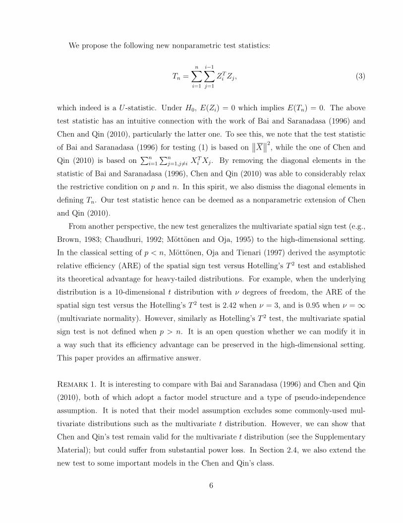
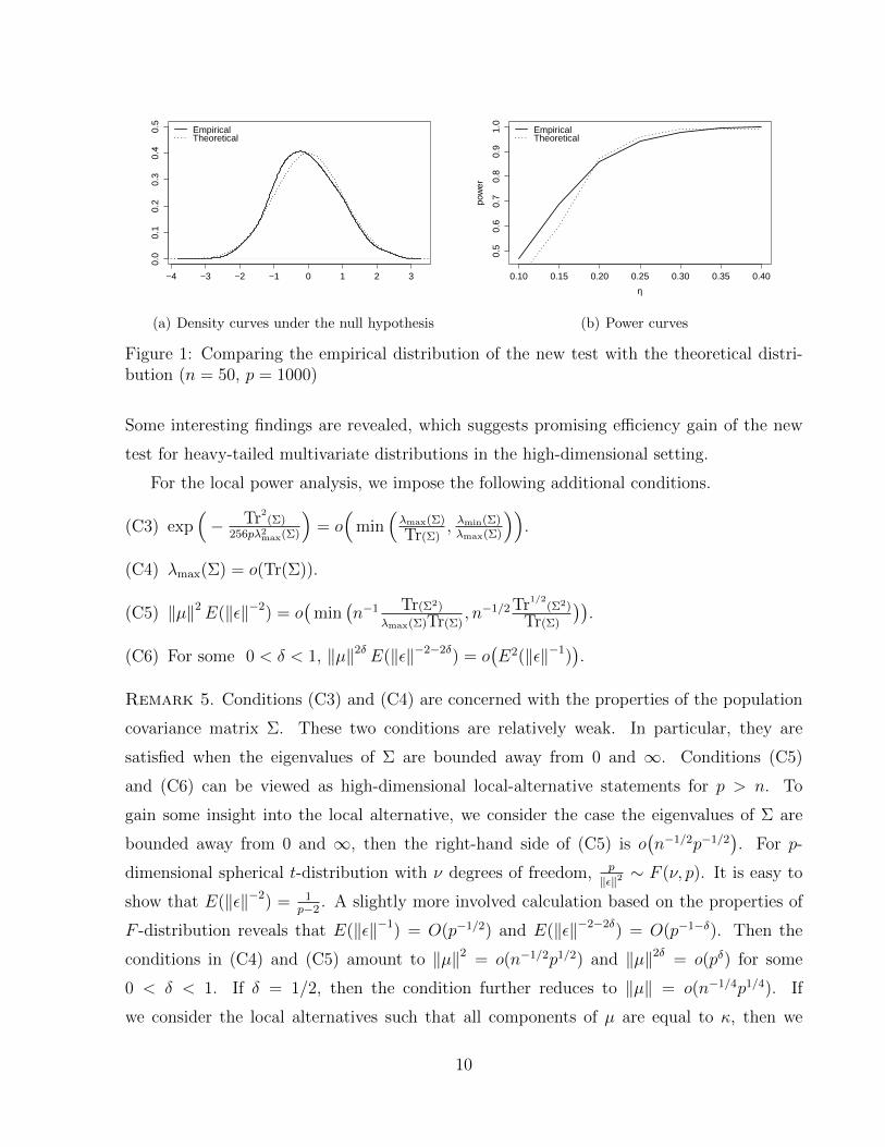
In Figure 1(a), we plot the empirical distribution of Tn√n(n−1)

2Tr(B2)

and compare it with the

N(0, 1) density curve for n = 50, p = 1000, where the data are generated from the Np(0,Σ)

distribution with the (i, j)th entry of Σ equal to 0.8|i−j|. The two curves are very close

to each other, which suggests that the standard normal distribution provides a satisfactory

approximation of the null distribution.

2.3 Local power analysis

We now turn our attention to the power analysis of Tn under contiguous sequences of al-

ternative hypotheses. This analysis enables us to further investigate the asymptotic relative

efficiency of Tn with respect to Chen and Qin’s test (referred to as CQ test in the sequel).

9

−4 −3 −2 −1 0 1 2 3

0.0

0.1

0.2

0.3

0.4

0.5

EmpiricalTheoretical

(a) Density curves under the null hypothesis

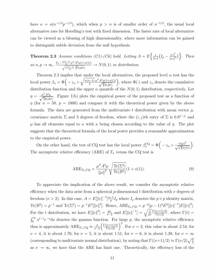
0.10 0.15 0.20 0.25 0.30 0.35 0.40

0.5

0.6

0.7

0.8

0.9

1.0

η

pow

er

EmpiricalTheoretical

(b) Power curves

Figure 1: Comparing the empirical distribution of the new test with the theoretical distri-bution (n = 50, p = 1000)

Some interesting findings are revealed, which suggests promising efficiency gain of the new

test for heavy-tailed multivariate distributions in the high-dimensional setting.

For the local power analysis, we impose the following additional conditions.

(C3) exp(− Tr2

(Σ)256pλ2max(Σ)

)= o(

min(λmax(Σ)

Tr(Σ), λmin(Σ)λmax(Σ)

)).

(C4) λmax(Σ) = o(Tr(Σ)).

(C5) ‖µ‖2E(‖ε‖−2) = o(

min(n−1 Tr(Σ2)

λmax(Σ)Tr(Σ), n−1/2 Tr1/2

(Σ2)

Tr(Σ)

)).

(C6) For some 0 < δ < 1, ‖µ‖2δ E(‖ε‖−2−2δ) = o(E2(‖ε‖−1)

).

Remark 5. Conditions (C3) and (C4) are concerned with the properties of the population

covariance matrix Σ. These two conditions are relatively weak. In particular, they are

satisfied when the eigenvalues of Σ are bounded away from 0 and ∞. Conditions (C5)

and (C6) can be viewed as high-dimensional local-alternative statements for p > n. To

gain some insight into the local alternative, we consider the case the eigenvalues of Σ are

bounded away from 0 and ∞, then the right-hand side of (C5) is o(n−1/2p−1/2

). For p-

dimensional spherical t-distribution with ν degrees of freedom, p

‖ε‖2 ∼ F (ν, p). It is easy to

show that E(‖ε‖−2) = 1p−2

. A slightly more involved calculation based on the properties of

F -distribution reveals that E(‖ε‖−1) = O(p−1/2) and E(‖ε‖−2−2δ) = O(p−1−δ). Then the

conditions in (C4) and (C5) amount to ‖µ‖2 = o(n−1/2p1/2) and ‖µ‖2δ = o(pδ) for some

0 < δ < 1. If δ = 1/2, then the condition further reduces to ‖µ‖ = o(n−1/4p1/4). If

we consider the local alternatives such that all components of µ are equal to κ, then we

10

have κ = o(n−1/4p−1/4), which when p > n is of smaller order of n−1/2, the usual local

alternative rate for Hotelling’s test with fixed dimension. The faster rate of local alternative

can be viewed as a blessing of high dimensionality, where more information can be gained

to distinguish subtle deviation from the null hypothesis.

Theorem 2.3 Assume conditions (C1)-(C6) hold. Letting A = E

1‖εi‖

(Ip − εiε

Ti

‖εi‖2)

. Then

as n, p→∞,Tn−n(n−1)

2µTA2µ(1+o(1))√

n(n−1)2

Tr(B2)→ N(0, 1) in distribution.

Theorem 2.3 implies that under the local alternatives, the proposed level α test has the

local power βn = Φ(− zα +

√n(n−1)

2µTA2µ(1+o(1))√

Tr(B2)

), where Φ(·) and zα denote the cumulative

distribution function and the upper α quantile of the N(0, 1) distribution, respectively. Let

η = µTA2µ√Tr(B2)

. Figure 1(b) plots the empirical power of the proposed test as a function of

η (for n = 50, p = 1000) and compare it with the theoretical power given by the above

formula. The data are generated from the multivariate t distribution with mean vector µ,

covariance matrix Σ and 3 degrees of freedom, where the (i, j)th entry of Σ is 0.8|i−j| and

µ has all elements equal to κ with κ being chosen according to the value of η. The plot

suggests that the theoretical formula of the local power provides a reasonable approximation

to the empirical power.

On the other hand, the test of CQ test has the local power βCQn = Φ

(− zα + n‖µ‖2√

2Tr(Σ2)

).

The asymptotic relative efficiency (ARE) of Tn versus the CQ test is

ARETn,CQ =µTA2µ

‖µ‖2

√Tr(Σ2)

Tr(B2)(1 + o(1)). (9)

To appreciate the implication of the above result, we consider the asymptotic relative

efficiency when the data arise from a spherical p-dimensional t distribution with ν degrees of

freedom (ν > 2). In this case, A = E[‖ε‖−1]p−1pIp where Ip denotes the p×p identity matrix,

Tr(B2) = p−1 and Tr(Σ2) = p−1E2[‖ε‖2]. Hence, ARETn,CQ = p−2(p − 1)2E2[‖ε‖−1]E[‖ε‖2].

For the t distribution, we have E[‖ε‖2] = pνν−2

and E[‖ε‖−1] =√

2pν

Γ((ν+1)/2)Γ(ν/2)

, where Γ(t) =∫∞0ut−1e−udu denotes the gamma function. For large p, the asymptotic relative efficiency

thus is approximately ARETn,CQ ≈ 2ν−2

(Γ((ν+1)/2)

Γ(ν/2)

)2

. For ν = 3, this value is about 2.54; for

ν = 4, it is about 1.76; for ν = 5, it is about 1.51; for ν = 6, it is about 1.38; for ν = ∞(corresponding to multivariate normal distribution), by noting that Γ((ν+1)/2) ≈ Γ(ν/2)

√ν2

as ν → ∞, we have that the ARE has limit one. Theoretically, the efficiency loss of the

11

new test under multivariate normality is little, but the efficiency gain can be substantial

for heavy-tailed distribution. Recall that for ν = 3, the ARE of the classical spatial sign

test versus Hotelling’s T 2 is 2.02 for p = 3 and 2.09 for p = 10 in the fixed dimensional

case. This suggests that nonparametric test may have more substantial power gain in the

high-dimensional case.

2.4 Extensions to beyond the elliptical distribution family

In this paper, we focus on the family of elliptical distributions because its popularity and

flexibility for modeling non-normal multivariate data. Our results have the potential to

extend to some useful multivariate distributions beyond the family of elliptical distributions.

One such class of distributions are those generated from the symmetric independent

component models (e.g., Ilmonen and Paindaveine, 2011). That is,

Xi = µ+ ΓZi, (10)

where Γ is a full rank p × p positive definite matrix; Zi = (Zi1, . . . , Zip)′ has independent

components Zij and Zij is symmetric about zero. The independent components model as-

sumes that the observed random vector can be written as linear combinations of independent

random variables. This model has received broad attentions in signal processing and ma-

chine learning (Hyvarinen, Karhunen and Oja, 2001). For example, independent component

analysis with exponential power marginal density (p(x) ∝ exp(−|x|q) for some q > 0) is pop-

ular for analyzing image and sound signals. It is noted that this class of models encompass

many of the practically useful distributions from Bai and Saranadasa (1996) and Chen and

Qin (2010).

We assume that Zij are standardized such that V ar(Zij) = 1. Thus Var(Xi) = ΓΓT . We

also assume that Zij has a sub-exponential distribution with exponent α, that is, there exist

constants a > 0, b > 0 such that for all t > 0, P (|Zij| ≥ tα) ≤ a exp(−bt). If α = 1/2,

then Zij is sub-gaussian. The class of sub-exponential distributions include many practically

used heavy-tailed distributions. The fact that our proposed test is still valid for this class is

summarized in the following theorem, whose proof is given in the Supplementary Material.

Theorem 2.4 Assume (C1) and (C2) hold for model (10), E(Z4ij) ≤ c for some positive

12

constant c for all i, j, and Tr(Σ2) = o(Tr2(Σ)). Then Tn√n(n−1)

2Tr(B2)

→ N(0, 1) in distribution

under H0, as n, p→∞, where B has the same expression as in Lemma 2.1.

Another interesting extension of the elliptical distributions involves generating random

variables from (2) but allowing Ri to be negative and depend on Ui. This yields the so-called

family of generalized elliptical distributions. The asymptotic results of this paper also hold for

this class by observing that Xi‖Xi‖ = Ui

‖Ui‖ under H0. This class of models recently caught the

attentions of researchers in finance, see Branco and Dey (2001), Frahm (2004), among others.

A representative example of this class is the collection of multi-tail elliptical distributions,

where Ri is a positive random variable whose tail parameter depends on ΓUi (e.g., Kring et

al, 2009; Rachev et al, 2011). The multi-tail elliptical distributions are particularly useful

for modeling asset returns in finance.

Not surprisingly, generalizations to other multivariate distributions are possible although

a case-by-case consideration may be needed. Particularly, the requirement that the Ui in

(2) is uniformly distributed on the L2 sphere can be relaxed. For example, one possible

extension is to allow Ui to be from the class of distributions discussed in Gupta and Song

(1997) and Szablowski (1998). Concentration inequalities similar to that given in Lemma

A.2, which plays an important role in the proof, can be obtained for random vectors that

satisfy certain concentration of measure properties (El Karoui, 2009).

3 Numerical studies

3.1 Monte Carlo simulations

We compare the performance of the new test with four alternatives: the test of Chen and Qin

(CQ test, 2010), the test of Srivastava, Katayama and Kano (SKK test, 2013), the test based

on multiple comparison with Bonferroni correction (BF test), and the test based on multiple

comparison with FDR control (FDR test, Benjamini and Hochberg, 1995). The SKK test

is constructed using the inverse of the diagonalized version of the sample covariance matrix

and is computationally attractive as it involves a simple estimator for the asymptotic covari-

ance. The BF test controls the family error rate at 0.05 and the FDR test controls the false

discovery rate at 0.05. Both the BF test and FDR test are computed using the p-values from

the t tests for the marginal hypotheses and reject H0 if at least one marginal test is signifi-

13

cant. The performance of the five tests are evaluated on 1000 simulation runs. We consider

n = 20, 50 and p = 200, 1000 and 2000. To save space, we report the results for p = 1000

and 2000 here. The results for p = 50, 100 and 200 are reported in the Supplemental Material.

Example 1. In this example, random data were generated from Np(µ,Σ). We consider

three different choices for µ and three different choices for Σ = (σij).

The three choices for µ are: (1) the null hypothesis µ0 = (0, . . . , 0)T ; (2) the alternative

µ1 = (0.25, 0.25, . . . , 0.25)T ; and (3) the alternative µ2 = (µ21, . . . , µ2p)T with µ21 = . . . =

µ2 p3

= 0, µ2( p3

+1) = . . . = µ2( 2p3

) = 0.25 and µ2( 2p3

+1) = . . . = µ2p = −0.25. The three

choices for Σ are: (1) σii = 1 and σij = 0.2 (i 6= j); (2) σij = 0.8|i−j|; and (3) Σ = DRD,

where D = diag(d1, . . . , dp) with di = 2 + (p − i + 1)/p, R = (rij) with rii = 1 and

rij = (−1)i+j(0.2)|i−j|0.1

for i 6= j. In the tables, we denote these three choices for Σ by Σ1,

Σ2 and Σ3, respectively. It is noted that Σ3 was considered in Srivastava, Katayama and

Kano (2013).

Table 1 summarizes the simulations results for different choices of Σ, µ, n and p. We

observe that the five tests have nominal levels reasonably close to 0.05, especially when

n = 50. For the alternative µ1, the performance of the new test is very close to that of the

CQ test and the SKK test, which are significantly better than the BF test and the FDR

test. The latter two tests have especially low power when n = 20. For the alternative µ2,

we first note that the BF test and the FRD test perform fine for Σ1 when n = 50 but has

significantly lower power in all other settings. We also observe that the new test, the CQ test

and the SKK test perform similarly for Σ3; the new test has somewhat better performance

for Σ1; and the SKK test has somewhat better performance for Σ2 for p = 1000.

[Table 1 is about here]

Example 2. We simulate Xi from a p-variate t distribution with mean vector µ, covariance

matrix Σ and 3 degrees of freedom. The choices of µ and Σ are set to be the same as those

in Example 1. The distribution is heavy-tailed in this example.

We summarize the simulation results in Table 2. Both the new test and the CQ test have

empirical levels close to 0.05 under the null hypothesis µ0 while the other three tests tend to

be conservative. In this example, the BF test and FDR test perform unsatisfactorily under

the alternatives µ1 and µ2. It is observed that the new test has the best power performance

in all settings; which is often substantially higher than (sometimes more than twofold) the

14

second best performed test (the CQ test in this example). For example, the new test (and

the CQ test) has power 0.83 (and 0.36) for the setting with µ = µ2, Σ = Σ1, n = 20 and

p = 2000; 0.98 (and 0.47) for the setting with µ = µ1, Σ = Σ2, n = 50 and p = 1000; 0.88

(and 0.51) for the setting with µ = µ1, Σ = Σ3, n = 20 and p = 2000.

[Table 2 is about here]

Example 3. We simulate Xi from a scale mixture of two multivariate normal distributions

0.9∗Np(µ,Σ)+0.1∗Np(µ, 9Σ), where we consider the same choices of µ and Σ as in Example

1. The distribution in this example also has heavy tails.

We summarize the simulation results in Table 3. Similarly as in Example 2, the new test

significantly outperforms the four contending approaches. For example, the new test (and

the CQ test) has power 0.88 (and 0.49) for the setting with µ = µ2, Σ = Σ1, n = 20 and

p = 2000; 0.80 (and 0.42) for the setting with µ = µ2, Σ = Σ2, n = 50 and p = 1000; 0.91

(and 0.70) for the setting with µ = µ1, Σ = Σ3, n = 20 and p = 2000.

[Table 3 is about here]

3.2 An application

Type 2 diabetes is one of the most common chronic diseases. Insulin resistance in skeletal

muscle, which is the major site of glucose disposal, is a prominent feature of Type 2 diabetes.

To study insulins ability to regulate gene expression, an experiment performed microarray

analysis using the Affymetrix Hu95A chip of human skeletal muscle biopsies from 15 diabetic

patients both before and after insulin treatment (Wu et al., 2007). The gene expression

alterations are promising to provide insights on new therapeutic targets for the treatment

of this common disease. Hence, we are interested in testing the hypothesis in (1), where µ

represents the average change of the gene expression level due to the treatment.

The underlying genetics of Type 2 diabetes were recognized to be very complex. It

is believed that Type 2 diabetes is resulted from interactions between many genetic fac-

tors and the environment. The data were normalized by quantile normalization. When

multiple probes are associated with the same gene, their expression values are consol-

idated by taking the average. In our analysis, we considered 2519 curated gene sets.

15

The gene sets we used are from the C2 collection of the GSEA online pathway databases

(http://www.broadinstitute.org/gsea/msigdb/collection details.jsp#C2). The largest gene

set contains 1607 genes, which makes the hypothesis testing problem a high-dimensional

one.

We applied both the new test and the CQ test at 5% significance level with the Bonferroni

correction to control the family-wise error rate at 0.05 level. For the CQ method, 520 gene

sets (20.64% of all candidates) are identified as significant; and for the new method, 954 gene

sets (37.87% of all candidates) are selected as significant. We observe that the significant

gene sets selected by the new test include those identified by the CQ test with only one

exception (HASLINGER B CLL WITH CHROMOSOME 12 TRISOMY).

Table 4 displays the top 10 significant gene sets identified by the two tests and their

corresponding test statistics values. The “NA” values in the table correspond to gene sets

in the top 10 list of one test but not the other. We observe these two lists share 7 common

gene sets. Among these seven gene sets, ZWANG CLASS 2 TRANSIENTLY INDUCED

BY EGF, NAGASHIMA EGF SIGNALING UP, AMIT EGF RESPONSE 60 HELA,

AMIT SERUM RESPONSE 40 MCF10A and AMIT SER UM RESPONSE 60 MCF10A are

known to be biologically related to insulin effect on human cells. We also observe that for 9

out of the top 10 gene sets, the new test has a smaller p-value than the CQ test does. The

gene set SEMENZA HIF1 TARGETS is only on the top ten list of the new test and was also

found to be biologically related to insulin effect on human cells. Most of those significant

gene sets are induced by Epidermal growth factor (EGF) or insulin-like growth factor (IGF).

[Table 4 is about here]

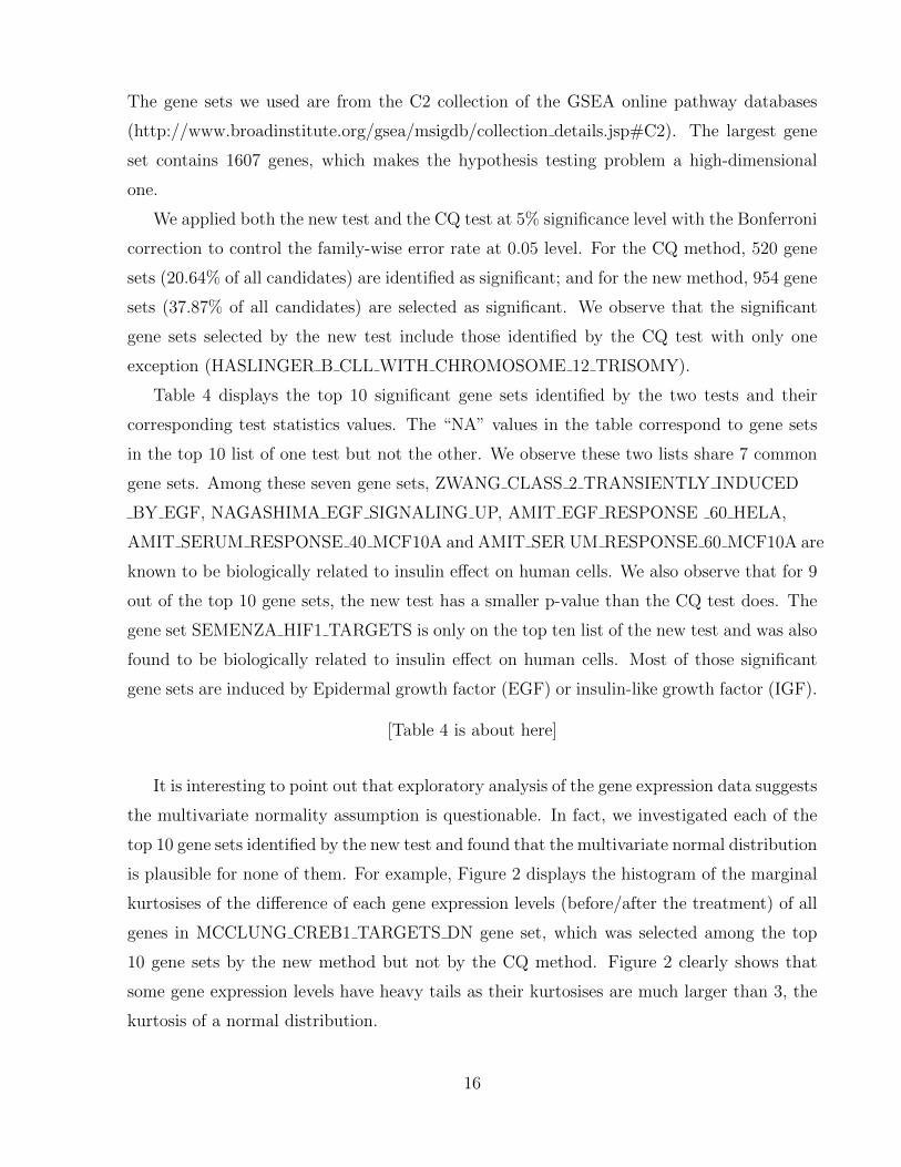
It is interesting to point out that exploratory analysis of the gene expression data suggests

the multivariate normality assumption is questionable. In fact, we investigated each of the

top 10 gene sets identified by the new test and found that the multivariate normal distribution

is plausible for none of them. For example, Figure 2 displays the histogram of the marginal

kurtosises of the difference of each gene expression levels (before/after the treatment) of all

genes in MCCLUNG CREB1 TARGETS DN gene set, which was selected among the top

10 gene sets by the new method but not by the CQ method. Figure 2 clearly shows that

some gene expression levels have heavy tails as their kurtosises are much larger than 3, the

kurtosis of a normal distribution.

16

histogram of kurtosis

kurtosis

Fre

qu

en

cy

2 4 6 8 10

01

23

45

67

Figure 2: The histogram of marginal kurtosises for all genes in MC-CLUNG CREB1 TARGETS DN gene set.

4 Conclusion and discussions

The paper proposes a new spatial sign based nonparametric test for testing a hypothesis

about the location parameter of a high-dimensional random vector. The goal is to improve

the power performance when the underlying distribution of the data deviates from multi-

variate normality. We investigate the asymptotic properties of the new test and compare it

with alternative tests based on extending Hotelling’s T 2 test. A remarkable finding is the

power improvement in the large p setting can be more substantial than that in the classical

fixed p setting. The proposed test can be used as a basic building block to develop nonpara-

metric tests in other important settings such as testing for sparse alternative or testing a

hypothesis on coefficients in high-dimensional factorial designs (Zhong and Chen, 2011). A

spatial sign based test was proposed for sphericity when p = O(n2) in Zou et al. (2014), and

spatial sign tests were proposed for testing uniformity on the unit sphere and other related

null hypotheses when p/n→ c for some positive constant c in Paindaveinez and Verdebout

(2013). The techniques related to sign tests have the potential to be used to develop the

high-dimensional theory for other classical nonparametric multivariate testing procedures,

such as those based on spatial sign ranks (e.g., Mottonen and Oja, 1995) and ranks (e.g.,

Hallin and Davy Paindaveine, 2006).

For reasons discussed in the introduction section, detecting the significance of a gene

set is often of independent interest. In particular, finding significant gene sets/pathways

17

can improve our understanding of the biological processes associated with a specific disease.

The proposed method can also be incorporated into a multi-step procedure, in combination

with various gene-level testing procedures and multiple tests correction methods, to further

identify a short list of top genes for the biologists. This kind of multi-step procedure is

expected to have better power to identify important individual genes as the gene set acts as

a dimension reduction from potentially thousands of genes.

References

[1] Bai, Z., and Sarandasa, H. (1996), “Effect of High Dimension: By an Example of a TwoSample Problem”. Statistica Sinica, 6, 311-329.

[2] Benjamini, Yoav, and Hochberg, Yosef. (1995), ”Controlling the False Discovery Rate:a Practical and Powerful Approach to Multiple Testing”. Journal of the Royal StatisticalSociety, Series B, 57, 289?00.

[3] Bickel, P.J. and Levina, E. (2008), “Covariance Regularization by Thresholding”. Annalsof Statistics, 36, 2577-2604.

[4] Branco, M.D. and Dey, D.K. (2001), “A General Class of Multivariate Skew-ellipticalDistributions”. Journal of Multivariate Analysis, 79, 99-113.

[5] Brown, B. M. (1983), “Statistical Uses of the Spatial Median,” Journal of the RoyalStatistical Society, Series B, 45, 25-30.

[6] Cai, T., Liu, W., and Xia, Y. (2014) “Two-sample Test of High Dimensional Meansunder Dependence”, Journal of the Royal Statistical Society, Series B, 76, 349-372.

[7] Chaudhuri, P. (1992), “Multivariate Location Estimation Using Extension of R-estimates through U-statistics Type Approach,” Annals of Statistics, 20, 897-916.

[8] Chen, S. X., and Qin, Y. L. (2010), “A Two-sample Test for High-dimensional Datawith Application to Gene-Set Testing,” Annals of Statistics, 38, 808-835.

[9] Cook, R. D., Forzani, L., and Rothman, A. J. (2012), “Estimating Sufficient Reductionsof the Predictors in Abundant High-dimensional Regressions” Annals of Statistics, 40,353?84.

[10] El Karoui, N. (2009), “Concentration of Measure and Spectra of Random Matrices:with Applications to Correlation Matrices, Elliptical Distributions and Beyond,” TheAnnals of Applied Probability, 19, 2362-2405.

[11] Fang, K. T., Kotz, S., and Ng, K. W. (1990), Symmetric Multivariate and RelatedDistributions, Chapman and Hall, London.

18

[12] Frahm, G. 2004. “Generalized Elliptical Distributions: Theory and Applications”. Ph.D.thesis, University of Cologne, Germany.

[13] Gupta, A. K. , and Song, D. (1997), “Lp-norm Spherical Distributions”, Journal ofStatistical Planning and Inference, 100, 241-260.)

[14] Hallin, M., and Paindaveine, D. (2006), “Semiparametrically Efficient Rank-based Infer-ence for Shape I. Optimal Rank-based Tests for Sphericity”, The Annals of Statistics,34, 2707-2756.

[15] Hall, P., and Heyde, C. (1980), Martingale Limit Theory and Applications, AcademicPress, New York.

[16] Hall, P. and Jin, J. (2010), “Innovated Higher Criticism for Detecting Sparse Signals inCorrelated Noise”, The Annals of Statistics, 38, 1686-1732.

[17] Hyvarinen, A., Karhunen, J. ,and Oja, E. (2001), Independent Component Analysis,John Wiley & Sons, New York.

[18] Ilmonen, P., and Paindaveine, D. (2011), “Semiparametrically Efficient Inference basedon Signed Ranks in Symmetric Independent Component Models”, Annals of Statistics,39, 2448-2476.

[19] Kring, S., Rachev, S. T., Hchsttter, M., Fabozzi, F. J. and Bianchi, M. L. (2009), ‘Multi-tail Generalized Elliptical Distributions for Asset Returns”, The Econometrics Journal,12, 272?91.

[20] Lee, S. H. , Limb, J., Li, E. Vannuccid, M., Petkova, E. (2012), “Order test for high-dimensional two-sample means”, Journal of Statistical Planning and Inference usingrandom subspaces, 142, 2719-2725.

[21] Ledoux, M. (2001). The Concentration of Measure Phenomenon. American Mathemat-ical Society. Providence, Rhode Island.

[22] Mcneil, A. J., Frey, R., and Embrechts, P. (2005), Quantitative Risk Management:Concepts, Techniques and Tools, Princeton University Press, Princeton, NJ.

[23] Mottonen, J., and Oja, H. (1995), “Multivariate Spatial Sign and Rank Methods,”Journal of Nonparametric Statistics, 5, 201-213.

[24] Mottonen, J., Oja, H., and Tienari, J. (1997), “On the Efficiency of Multivariate SpatialSign and Rank Tests,” Annals of Statistics, 25, 542-552.

[25] Oja, H. (2010), Multivariate Nonparametric Methods with R, Springer.

[26] Paindaveine, D. and Verdebout, T. (2013), “Universal Asymptotics for High-dimensionalSign Tests”, technical report, Universite libre de Bruxellesz. .

[27] Pan, G. M and Zhou, W. (2011), “Central Limit Theorem for Hotelling’s T 2 Statisticunder Large Dimension”, Annals of Applied Probability., 21, 1860-1910.

19

[28] Purdom, E., and Holmes, S.P. (2005), “Error Distribution for Gene Expression Data”,Statistical Applications in Genetics and Molecular Biology, 4, Article 16.

[29] Rachev, S. T., Kim, Y. S., Bianchi, M. L. and Fabozzi, F. J. (2011), ‘Multi-Tail t-Distribution”, in Financial Models with Levy Processes and Volatility Clustering, JohnWiley & Sons., Hoboken, NJ, USA.

[30] Schmidt, R. (2002), “Tail Dependence for Elliptically Contoured Distributions,” Math-ematical Methods of Operations Research, 55, 301-327.

[31] Srivastava, M. (2009), “A Test for the Mean Vector with Fewer Observations than theDimension under Non-normality”, Journal of Multivariate Analysis, 100, 386- 402.

[32] Srivastava, M. S., and Du, M. (2008), “A Test for the Mean Vector with Fewer Obser-vations than the Dimension,” Journal of Multivariate Analysis, 99, 386-402.

[33] Srivastava, M. S., Katayama, S., and Kano, Y. (2013), “A two sample test in highdimensional data,” Journal of Multivariate Analysis, 114, 349-358.

[34] Szabowski, P. J. (1998), “Uniform Distributions on Spheres in Finite-dimensional Lαand Their Generalization”, Journal of Multivariate Analysis, 64, 103-117.

[35] Thulin, M. (2014). 11A high-dimensional two-sample test for the mean using randomsubspaces”. Computational Statistics & Data Analysis. 74, 26 - 38.

[36] Vo, T., Phan, J., Huynh, K., and Wang, M. (2007), “Reproducibility of DifferentialGene Detection across Multiple Microarray Studies”, In Engineering in Medicine andBiology Society, 2007. EMBS 2007. 29th Annual International Conference of the IEEE,4231?234.

[37] Wu, X., Wang, J., Cui, X., Maianu, L. et al., (2007), “The Effect of Insulin on Expressionof Genes and Biochemical Pathways in Human Skeletal Muscle,” Endocrine, 31, 5-17.

[38] Zhong, P. S., and Chen, S. X. (2011), “Tests for High Dimensional Regression Coef-ficients with Factorial Designs”, Journal of the American Statistical Association, 106,260-274.

[39] Zhong, P. S., Chen, S. X. and Xu, M. Y. (2013), “Tests Alter- native to Higher Criticismfor High Dimensional Means under Sparsity and Column-wise Dependence”, The Annalsof Statistics, 41, 2703-3110.

[40] Zou, C. L., Peng, L. H. and Wang, Z. J. (2014), “Multivariate Sign-based High-dimensional Tests for Sphericity”, Biometrika, 101, 229-236.

20

Appendix: Technical proofs

Appendix 1: Some useful lemmas

We present below several useful technical lemmas, the proof for which can be found in the

online supplementary material.

Lemma A.1 Let U = (U1, . . . , Up)T be a random vector uniformly distributed on the unit

sphere in Rp. Then

(1) E(U) = 0, V ar(U) = p−1Ip, E(U4j ) = 3

p(p+2), ∀ j, and E(U2

j U2k ) = 1

p(p+2)for j 6= k.

(2) Let M be a deterministic real-valued matrix. Assume that ‖M‖2 ≤ k, where ‖M‖2

denotes the spectral norm of M . Then, ∀ t > 0, P(∣∣UTMU − p−1Tr(M)

∣∣ > t)≤ 2 exp

(−

(p−1)(t−cp)2

8k2

), where cp =

√8πk2

p−1.

Lemma A.2 (A concentration inequality) Assume W = ΓU , where U is uniformly dis-

tributed on the unit sphere in Rp. Let Ω = ΓΓT and consider the event A =Tr(Ω)

2p≤ ‖W‖2 ≤

3Tr(Ω)2p

. Then P (A) ≥ 1− c1 exp

(− Tr2

(Σ)128pλ2max(Σ)

), for all p > 1, where c1 = 2 exp(π/2) is a

finite constant.

Lemma A.3 For any p-dimensional vectors X and µ, we have (1)∥∥∥ X−µ‖X−µ‖ −

X‖X‖

∥∥∥ ≤ 2 ‖µ‖‖X‖ ;

and (2)∥∥∥ X−µ‖X−µ‖ −

X‖X‖ −

1‖X‖

(Ip − XXT

‖X‖2)µ∥∥∥ ≤ c2

‖µ‖1+δ

‖X‖1+δ , for all 0 < δ < 1, where c2 is a

constant that does not depend on X or µ.

Lemma A.4 Let B be the matrix defined in Lemma 2.1. Assume condition (C3) holds, then

λmax(B) ≤ 2λmax(Σ)

Tr(Σ)(1 + o(1)).

Lemma A.5 Let A be the matrix defined in Theorem 2.3 and D = E

1‖ε1‖2

(Ip − ε1εT1

‖ε1‖2

),

then λmax(A) ≤ E(‖ε1‖−1) and λmax(D) ≤ E(‖ε1‖−2). Furthermore, if conditions (C3) and

(C4) hold, then λmin(A) ≥ 1√3E(‖ε1‖−1)(1− o(1)).

Appendix 2: Proof of main theorems

We use c or C to denote generic positive constants, which may vary from line to line.

21

Proof of Theorem 2.2. Let S2n = V ar(Tn) = n(n−1)

2Tr(B2) = n(n−1)

2E

(ZT1 Z2)2

. Let

V 2n =

∑ni=2 E(Y 2

i |Z1, . . . , Zi−1) and Yi =∑i−1

j=1 ZTi Zj. To apply the martingale central limit

theorem (Hall and Heyde, 1980), it is sufficient to check two conditions:

S−4n

n∑i=2

E(Y 4i ) → 0 as n, p→∞, (A.1)

S−2n V 2

n → 1 in probability as n, p→∞. (A.2)

To check (A.1), note that under H0,

E(Y 4i ) = E

( i−1∑j=1

ZTi Zj

)4

=i−1∑j=1

E

(ZTi Zj)

4

+ 3∑

1≤j,k≤i−1j 6=k

E

(ZTi Zj)

2(ZTi Zk)

2

= (i− 1)E

(ZT1 Z2)4

+ 3(i− 1)(i− 2)E

(ZT

1 Z2)2(ZT1 Z3)2

.

Hence,∑n

i=1E(Y 4i ) ≤ c

[n2E

(ZT

1 Z2)4

+ n3E

(ZT1 Z2)2(ZT

1 Z3)2]≤ cn3E

(ZT

1 Z2)4

by

Holder’s inequality. By Lemma 2.1, we have E

(ZT1 Z2)4

= o(nE2

(ZT

1 Z2)2)

. Therefore,

(A.1) holds.

To prove (A.2), it is sufficient to verify that E(V 2n−S2

n)2

S4n

→ 0 as n, p → ∞. We write

V 2n =

∑ni=2 Vni, where Vni = E(Y 2

i |Z1, . . . , Zi−1). We have

Vni =i−1∑j=1

i−1∑k=1

E(ZTi ZjZ

Ti Zk|Z1, . . . , Zi−1) =

i−1∑j=1

i−1∑k=1

Tr(ZjZTk B) =

i−1∑j=1

i−1∑k=1

ZTj BZk

= 2∑

1≤j<k≤i−1

ZTj BZk +

i−1∑j=1

ZTj BZj.

If j1 ≤ k1 and j2 ≤ k2, then

E(ZTj1BZk1Z

Tj2BZk2

)= E

(ZT

1 BZ1)2Ij1 = k1 = j2 = k2+ E2

(ZT

1 BZ1

)Ij1 = k1 6= j2 = k2

+E

(ZT1 BZ2)2

Ij1 = j2, k1 = k2, j1 < k1.

22

Therefore, for i1 ≤ i2,

E(Vni1Vni2

)= 4

∑1≤j<k≤i1−1

E

(ZT1 BZ2)2

+

i1−1∑j=1

i2−1∑k=1

E2(ZT

1 BZ1

)+

i1−1∑j=1

[E

(ZT1 BZ1)2

− E2(ZT

1 BZ1)]

= 2(i1 − 1)(i1 − 2)E

(ZT1 BZ2)2

+ (i1 − 1)(i2 − 1)E2

(ZT

1 BZ1

)+ (i1 − 1)V ar(ZT

1 BZ1).

Consequently,

E(V 4n ) = E

( n∑i=2

Vni)2

= 2∑

2≤i<j≤n

E(VniVnj) +n∑i=2

E(V 2ni)

= 2n∑i=2

(i− 1)(i− 2)(2n− 2i+ 1)E

(ZT1 BZ2)2

+

n∑i=2

(i− 1)(2n− 2i+ 1)V ar(ZT1 BZ1)

+n(n− 1)E

(ZT

1 BZ1

)/22

.

Note that E(ZT

1 BZ1

)= Tr(B2) and S2

n = n(n−1)2

Tr(B2). Hence,

E

(V 2n − S2

n)2

= E(V 4n )− S4

n

= 2n∑i=2

(i− 1)(i− 2)(2n− 2i+ 1)E

(ZT1 BZ2)2

+

n∑i=2

(i− 1)(2n− 2i+ 1)V ar(ZT1 BZ1)

≤ c[n4E

(ZT

1 BZ2)2

+ n3E

(ZT1 BZ1)2

].

Hence, a sufficient condition for S−4n E(V 2

n − S2n)2 → 0 is

n4E

(ZT1 BZ2)2

+n3E

(ZT1 BZ1)2

n4E2ZT1 BZ1

→ 0.

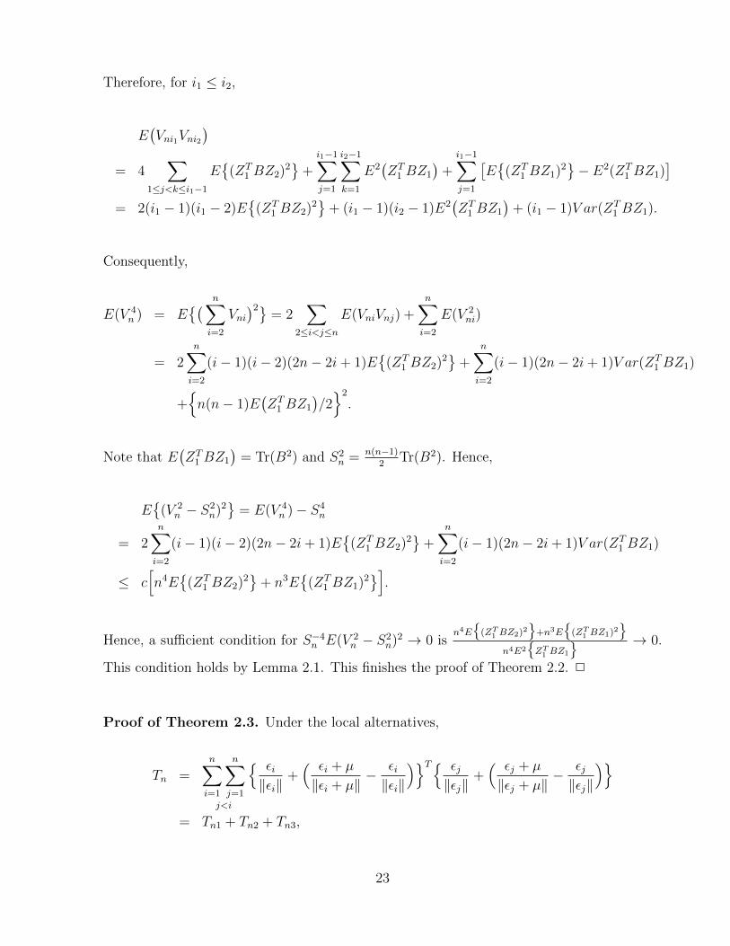
This condition holds by Lemma 2.1. This finishes the proof of Theorem 2.2. 2

Proof of Theorem 2.3. Under the local alternatives,

Tn =n∑i=1

n∑j=1

j<i

εi‖εi‖

+( εi + µ

‖εi + µ‖− εi‖εi‖

)T εj‖εj‖

+( εj + µ

‖εj + µ‖− εj‖εj‖

)= Tn1 + Tn2 + Tn3,

23

where Tn1 =∑n

i=1

∑nj=1

j<i

εTi εj‖εi‖‖εj‖ , Tn2 =

∑ni=1

∑nj=1

j 6=i

(εi+µ‖εi+µ‖−

εi‖εi‖

)Tεj‖εj‖ , and Tn3 =

∑ni=1

∑nj=1

j<i

(εi+µ‖εi+µ‖−

εi‖εi‖

)T(εj+µ

‖εj+µ‖ −εj‖εj‖

). By Theorem 2.2, Tn1/

√n(n−1)

2Tr(B2)→ N(0, 1).

To analyze Tn2, we write Tn2 = Tn21 + Tn22, where Tn21 =∑

i<j

(εi+µ‖εi+µ‖ −

εi‖εi‖

)Tεj‖εj‖ and

Tn22 =∑

j<i

(εi+µ‖εi+µ‖ −

εi‖εi‖

)Tεj‖εj‖ . Note that E(Tn21) = 0, and

E(T 2n21) =

∑i1<j1

∑i2<j2

E( εi1 + µ

‖εi1 + µ‖− εi1‖εi1‖

)T εj1‖εj1‖

εTj2‖εj2‖

( εi2 + µ

‖εi2 + µ‖− εi2‖εi2‖

)=

∑i1<j

∑i2<j

E( εi1 + µ

‖εi1 + µ‖− εi1‖εi1‖

)TB( εi2 + µ

‖εi2 + µ‖− εi2‖εi2‖

)≤ λmax(B)

∑i1<j

∑i2<j

E 4 ‖µ‖2

‖εi1‖ ‖εi2‖

≤ 8

λmax(Σ)

Tr(Σ)(1 + o(1)) ‖µ‖2

∑i<j

E(‖εi‖−2) +∑i1<j

∑i2<j

E2(‖εi1‖−1)

≤ O(n3 ‖µ‖2)λmax(Σ)

Tr(Σ)E(‖ε‖−2),

where the first inequality uses Lemma A.3, and the second inequality uses Lemma A.4. In

the derivation in Lemma 2.1, we derived that Tr(B2) ≥ 49

Tr(Σ2)

Tr2(Σ)

(1− o(1)). Hence, it follows

by condition (C5) that

E(T 2n21)

n(n−1)2

Tr(B2)≤ O(n ‖µ‖2)

λmax(Σ)Tr(Σ)

Tr(Σ2)E(‖ε‖−2) = o(1).

This implies Tn21/√

n(n−1)2

Tr(B2) = op(1). Similarly, Tn22/√

n(n−1)2

Tr(B2) = op(1).

Finally, we analyze Tn3. Denote

Tn31 =n(n− 1)

2E( ε1 + µ

‖ε1 + µ‖

)TE( ε2 + µ

‖ε2 + µ‖

),

Tn32 =∑j 6=i

E( εi + µ

‖εi + µ‖

)T εj + µ

‖εj + µ‖− εj‖εj‖

− E( εj + µ

‖εj + µ‖

),

Tn33 =∑j<i

εi + µ

‖εi + µ‖− εi‖εi‖

− E( εi + µ

‖εi + µ‖

)T εj + µ

‖εj + µ‖− εj‖εj‖

− E( εj + µ

‖εj + µ‖

).

24

Then it follows that

Tn3 =n∑i=1

n∑j=1

j<i

[E( εi + µ

‖εi + µ‖

)+ εi + µ

‖εi + µ‖− εi‖εi‖

− E( εi + µ

‖εi + µ‖

)]T

×[E( εj + µ

‖εj + µ‖

)+ εj + µ

‖εj + µ‖− εj‖εj‖

− E( εj + µ

‖εj + µ‖

)]= Tn31 + Tn32 + Tn33.

To analyze Tn31, by Lemma A.3 (2), we can write E(

ε1+µ‖ε1+µ‖

)= −Aµ + E(Q1), where

Q1 = ε1+µ‖ε1+µ‖ −

ε1‖ε1‖ + 1

‖ε1‖

(Ip − ε1εT1

‖ε1‖2)µ satisfies E(‖Q1‖2) ≤ c3 ‖µ‖2+2δ E

(‖ε1‖−2−2δ ) for all

0 < δ < 1, where c3 is a constant that does not depend on ε1 or µ. Hence,

E( ε1 + µ

‖ε1 + µ‖

)TE( ε2 + µ

‖ε2 + µ‖

)= µTA2µ− µTAE(Q1)− µTAE(Q2) + E(Q1)TE(Q2).

Note that by Lemma A.5 and condition (C6), the last three terms on the right-hand side of

the above expression are bounded by

2c1/23 ‖µ‖

1+δ∥∥µTA∥∥ · E1/2

(‖ε1‖−2−2δ

)+ c3 ‖µ‖2+2δ E

(‖ε1‖−2−2δ

)≤ c ‖µ‖2 o

(E2(‖ε1‖−1)

)= o(µTA2µ).

Therefore, Tn31 = n(n−1)2

µTA2µ(1 + o(1)).

To evaluate Tn32, we observe that E(Tn32) = 0 and that

E(T 2n32) = O(n3)E

( ε2 + µ

‖ε2 + µ‖

)TE( ε1 + µ

‖ε1 + µ‖− ε1‖ε1‖

− E( ε1 + µ

‖ε1 + µ‖

))( ε1 + µ

‖ε1 + µ‖− ε1‖ε1‖

− E( ε1 + µ

‖ε1 + µ‖

))TE( ε3 + µ

‖ε3 + µ‖

).

Note that by Lemma A.3 (2),

ε1 + µ

‖ε1 + µ‖− ε1‖ε1‖

− E( ε1 + µ

‖ε1 + µ‖

)= −

1

‖ε1‖

(Ip −

ε1εT1

‖ε1‖2

)− A

µ+ (Q1 − E(Q1)).

25

Applying the above decomposition, we obtain

λmax

[E( ε1 + µ

‖ε1 + µ‖− ε1‖ε1‖

− E( ε1 + µ

‖ε1 + µ‖

))( ε1 + µ

‖ε1 + µ‖− ε1‖ε1‖

− E( ε1 + µ

‖ε1 + µ‖

))T]≤ 2 ‖µ‖2 λmax(D) + C ‖µ‖2+2δ E

(‖ε1‖−2−2δ

)≤ 2 ‖µ‖2E

(‖ε1‖−2 )+ C ‖µ‖2+2δ E

(‖ε1‖−2−2δ ),

by Lemma A.5, where D = E

1‖ε1‖2

(Ip − ε1εT1

‖ε1‖2

). Therefore, by Lemma A.5, conditions

(C5), (C6), and observing that Tr(B2) ≥ 4Tr(Σ2)

9Tr2(Σ)

(1− o(1)), we have

E(T 2n32) ≤ O(n3)

2 ‖µ‖2E

(‖ε1‖−2 )+ C ‖µ‖2+2δ E

(‖ε1‖−2−2δ ) ‖µ‖2E2

(‖ε1‖−1 )

≤ O(n3) ‖µ‖4E2(‖ε1‖−2 ) = o(n2Tr(B2)).

Therefore, Tn32/√

n(n−1)2

Tr(B2) = op(1).

To evaluate Tn33, we observe that E(Tn33) = 0 and that

E(T 2n33)

= O(n2)E[ ε1 + µ

‖ε1 + µ‖− ε1‖ε1‖

− E( ε1 + µ

‖ε1 + µ‖

)T ε2 + µ

‖ε2 + µ‖− ε2‖ε2‖

− E( ε2 + µ

‖ε2 + µ‖

) ε2 + µ

‖ε2 + µ‖− ε2‖ε2‖

− E( ε2 + µ

‖ε2 + µ‖

)T ε1 + µ

‖ε1 + µ‖− ε1‖ε1‖

− E( ε1 + µ

‖ε1 + µ‖

)]≤ O(n2)

2 ‖µ‖2 λmax(D) + C ‖µ‖2+2δ E

(‖ε1‖−2−2δ

)×E[ ∥∥∥∥ ε1 + µ

‖ε1 + µ‖− ε1‖ε1‖

− E( ε1 + µ

‖ε1 + µ‖

)∥∥∥∥2 ]≤ O(n2)

2 ‖µ‖2 λmax(D) + C ‖µ‖2+2δ E

(‖ε1‖−2−2δ

)2

≤ O(n2) ‖µ‖4E2(‖ε1‖−2 ) = o

(n2Tr(B2)

)by Lemma A.5, conditions (C5) and (C6). Therefore, Tn33/

√n(n−1)

2Tr(B2) = op(1). Sum-

marizing the above, Tn3/√

n(n−1)2

Tr(B2) =n(n−1)

2µTA2µ(1+o(1))√

n(n−1)2

Tr(B2)+op(1). This finishes the proof.

2

26

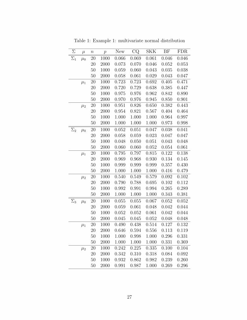
Table 1: Example 1: multivariate normal distribution

Σ µ n p New CQ SKK BF FDR

Σ1 µ0 20 1000 0.066 0.069 0.061 0.046 0.04620 2000 0.073 0.070 0.046 0.052 0.05350 1000 0.059 0.060 0.043 0.035 0.03850 2000 0.058 0.061 0.029 0.043 0.047

µ1 20 1000 0.723 0.723 0.692 0.405 0.47120 2000 0.720 0.729 0.638 0.385 0.44750 1000 0.975 0.976 0.962 0.842 0.89050 2000 0.970 0.976 0.945 0.850 0.901

µ2 20 1000 0.951 0.826 0.650 0.382 0.44320 2000 0.954 0.821 0.567 0.404 0.46450 1000 1.000 1.000 1.000 0.964 0.99750 2000 1.000 1.000 1.000 0.973 0.998

Σ2 µ0 20 1000 0.052 0.051 0.047 0.038 0.04120 2000 0.058 0.059 0.023 0.047 0.04750 1000 0.048 0.050 0.051 0.043 0.04850 2000 0.060 0.060 0.052 0.054 0.061

µ1 20 1000 0.795 0.797 0.815 0.122 0.13820 2000 0.969 0.968 0.930 0.134 0.14550 1000 0.999 0.999 0.999 0.357 0.43050 2000 1.000 1.000 1.000 0.416 0.479

µ2 20 1000 0.540 0.549 0.579 0.092 0.10220 2000 0.790 0.788 0.695 0.102 0.11250 1000 0.992 0.991 0.994 0.265 0.28950 2000 1.000 1.000 1.000 0.343 0.381

Σ3 µ0 20 1000 0.055 0.055 0.067 0.052 0.05220 2000 0.059 0.061 0.048 0.042 0.04450 1000 0.052 0.052 0.061 0.042 0.04450 2000 0.045 0.045 0.052 0.048 0.048

µ1 20 1000 0.490 0.438 0.514 0.127 0.13220 2000 0.646 0.594 0.556 0.113 0.11950 1000 1.000 0.998 1.000 0.296 0.33150 2000 1.000 1.000 1.000 0.331 0.369

µ2 20 1000 0.242 0.225 0.335 0.100 0.10420 2000 0.342 0.310 0.318 0.084 0.09250 1000 0.932 0.862 0.982 0.239 0.26050 2000 0.991 0.987 1.000 0.269 0.296

27

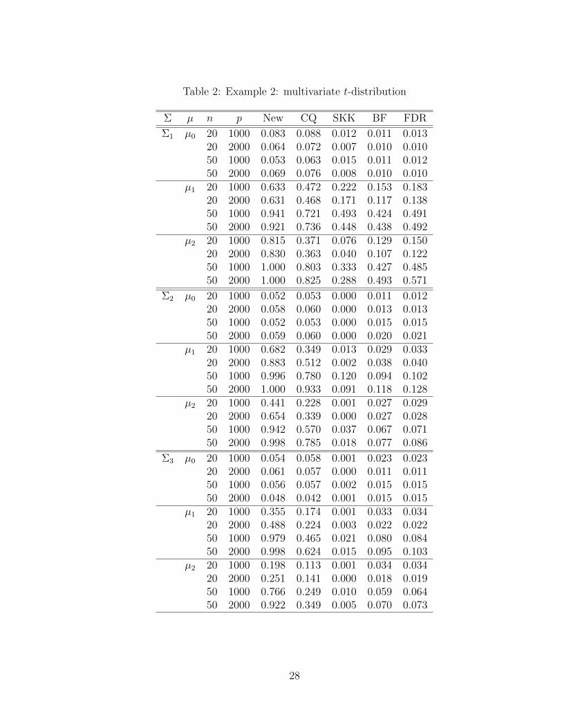
Table 2: Example 2: multivariate t-distribution

Σ µ n p New CQ SKK BF FDR

Σ1 µ0 20 1000 0.083 0.088 0.012 0.011 0.01320 2000 0.064 0.072 0.007 0.010 0.01050 1000 0.053 0.063 0.015 0.011 0.01250 2000 0.069 0.076 0.008 0.010 0.010

µ1 20 1000 0.633 0.472 0.222 0.153 0.18320 2000 0.631 0.468 0.171 0.117 0.13850 1000 0.941 0.721 0.493 0.424 0.49150 2000 0.921 0.736 0.448 0.438 0.492

µ2 20 1000 0.815 0.371 0.076 0.129 0.15020 2000 0.830 0.363 0.040 0.107 0.12250 1000 1.000 0.803 0.333 0.427 0.48550 2000 1.000 0.825 0.288 0.493 0.571

Σ2 µ0 20 1000 0.052 0.053 0.000 0.011 0.01220 2000 0.058 0.060 0.000 0.013 0.01350 1000 0.052 0.053 0.000 0.015 0.01550 2000 0.059 0.060 0.000 0.020 0.021

µ1 20 1000 0.682 0.349 0.013 0.029 0.03320 2000 0.883 0.512 0.002 0.038 0.04050 1000 0.996 0.780 0.120 0.094 0.10250 2000 1.000 0.933 0.091 0.118 0.128

µ2 20 1000 0.441 0.228 0.001 0.027 0.02920 2000 0.654 0.339 0.000 0.027 0.02850 1000 0.942 0.570 0.037 0.067 0.07150 2000 0.998 0.785 0.018 0.077 0.086

Σ3 µ0 20 1000 0.054 0.058 0.001 0.023 0.02320 2000 0.061 0.057 0.000 0.011 0.01150 1000 0.056 0.057 0.002 0.015 0.01550 2000 0.048 0.042 0.001 0.015 0.015

µ1 20 1000 0.355 0.174 0.001 0.033 0.03420 2000 0.488 0.224 0.003 0.022 0.02250 1000 0.979 0.465 0.021 0.080 0.08450 2000 0.998 0.624 0.015 0.095 0.103

µ2 20 1000 0.198 0.113 0.001 0.034 0.03420 2000 0.251 0.141 0.000 0.018 0.01950 1000 0.766 0.249 0.010 0.059 0.06450 2000 0.922 0.349 0.005 0.070 0.073

28

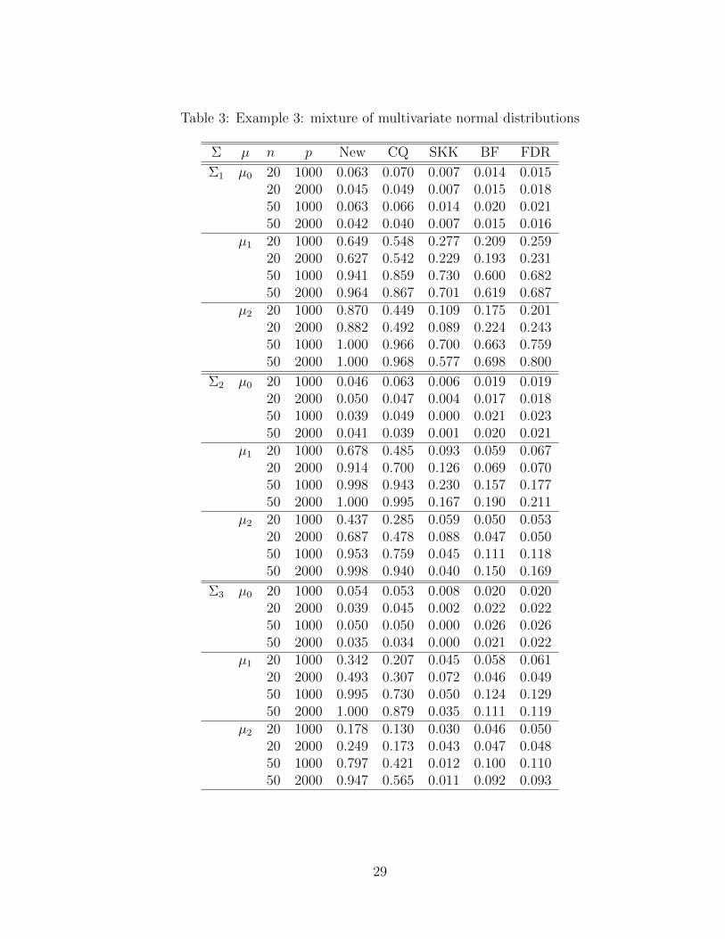
Table 3: Example 3: mixture of multivariate normal distributions

Σ µ n p New CQ SKK BF FDR

Σ1 µ0 20 1000 0.063 0.070 0.007 0.014 0.01520 2000 0.045 0.049 0.007 0.015 0.01850 1000 0.063 0.066 0.014 0.020 0.02150 2000 0.042 0.040 0.007 0.015 0.016

µ1 20 1000 0.649 0.548 0.277 0.209 0.25920 2000 0.627 0.542 0.229 0.193 0.23150 1000 0.941 0.859 0.730 0.600 0.68250 2000 0.964 0.867 0.701 0.619 0.687

µ2 20 1000 0.870 0.449 0.109 0.175 0.20120 2000 0.882 0.492 0.089 0.224 0.24350 1000 1.000 0.966 0.700 0.663 0.75950 2000 1.000 0.968 0.577 0.698 0.800

Σ2 µ0 20 1000 0.046 0.063 0.006 0.019 0.01920 2000 0.050 0.047 0.004 0.017 0.01850 1000 0.039 0.049 0.000 0.021 0.02350 2000 0.041 0.039 0.001 0.020 0.021

µ1 20 1000 0.678 0.485 0.093 0.059 0.06720 2000 0.914 0.700 0.126 0.069 0.07050 1000 0.998 0.943 0.230 0.157 0.17750 2000 1.000 0.995 0.167 0.190 0.211

µ2 20 1000 0.437 0.285 0.059 0.050 0.05320 2000 0.687 0.478 0.088 0.047 0.05050 1000 0.953 0.759 0.045 0.111 0.11850 2000 0.998 0.940 0.040 0.150 0.169

Σ3 µ0 20 1000 0.054 0.053 0.008 0.020 0.02020 2000 0.039 0.045 0.002 0.022 0.02250 1000 0.050 0.050 0.000 0.026 0.02650 2000 0.035 0.034 0.000 0.021 0.022

µ1 20 1000 0.342 0.207 0.045 0.058 0.06120 2000 0.493 0.307 0.072 0.046 0.04950 1000 0.995 0.730 0.050 0.124 0.12950 2000 1.000 0.879 0.035 0.111 0.119

µ2 20 1000 0.178 0.130 0.030 0.046 0.05020 2000 0.249 0.173 0.043 0.047 0.04850 1000 0.797 0.421 0.012 0.100 0.11050 2000 0.947 0.565 0.011 0.092 0.093

29

Table 4: The top 10 significant gene sets selected by the new test and the CQ testGene set New test CQ testZWANG CLASS 2 TRANSIENTLY INDUCED BY EGF 24.34 20.11NAGASHIMA EGF SIGNALING UP 22.44 17.01SHIPP DLBCL CURED VS FATAL DN 22.34 18.24WILLERT WNT SIGNALING 19.66 NAUZONYI RESPONSE TO LEUKOTRIENE AND THROMBIN 19.63 18.46PID HIF2PATHWAY 19.46 15.65PHONG TNF TARGETS UP 19.21 18.90AMIT EGF RESPONSE 60 HELA 18.64 16.38MCCLUNG CREB1 TARGETS DN 18.43 NASEMENZA HIF1 TARGETS 18.34 NAAMIT SERUM RESPONSE 40 MCF10A NA 15.98AMIT SERUM RESPONSE 60 MCF10A NA 15.43PLASARI TGFB1 TARGETS 1HR UP NA 15.00

30