multivariate and high dimensional visualizations
DESCRIPTION
Multivariate and High Dimensional Visualizations. Robert Herring. Articles Covered. Visualizing the Behavior of Higher Dimensional Dynamical Systems Rainer Wegenkittl, Helwig Loffelmann, and Eduard Groller Multivariate Visualization Using Metric Scaling Pak Chung Wong and R. Daniel Bergeron. - PowerPoint PPT PresentationTRANSCRIPT
Multivariate and High Dimensional Visualizations
Robert Herring
Articles Covered
Visualizing the Behavior of Higher Dimensional Dynamical Systems Rainer Wegenkittl, Helwig Loffelmann, and
Eduard Groller
Multivariate Visualization Using Metric Scaling Pak Chung Wong and R. Daniel Bergeron
Problem Addressed
Information gathered often contains multiple variables to be studied
Most visualization techniques focus on discrete statistical characteristics
These techniques are ill suited for visualizing continuous flow in high-dimensional space from dynamical systems
Statistical visualizations typically are not designed to show integral curves within a high-dimensional phase space
Visualizing the Behavior of Higher Dimensional Dynamical Systems
Visualizing Multidimensional Data
Multivariate data sets becoming common Data is either discrete of continuous Data can be spatially coherent or spatially
incoherent Data sets may consist of a collection of
sampled data Each sample is an n-dimensional data item Can be sampled from m-dimensional space Lm
n data set
Visualizing the Behavior of Higher Dimensional Dynamical Systems
Visualizing Multidimensional Data
Two important goals Identification of individual parameters Detection of regions and correlation of variables
Methods for visualizing high-dimensional data Attribute Mapping Geometric Coding Sonification Reduction of Dimension Parallel Coordinates
Visualizing the Behavior of Higher Dimensional Dynamical Systems

Attribute Mapping
Use geometric primitives, planes, etc. Most commonly used attribute used in
attribute mapping is color Most common color models RGB and HLS Advantages
Easy calculation/interpretation, many people familiar with color mapping
Disadvantages No unique order, requires legend Can only encode 3 variables 8% of population has some form of color
blindness
Visualizing the Behavior of Higher Dimensional Dynamical Systems
Geometric Coding
Use distinct geometric objects and map high-dimensional data to geometric features or attributes of these objects
Glyphs Icons Chernoff Faces Data Jacks m-Arm Glyph
Visualizing the Behavior of Higher Dimensional Dynamical Systems
Geometric Coding
Glyphs Utilized for interactive exploration of data sets Generic term for graphical entity whose
shape/appearance is modified by mapping data values to graphical attributes (length, shape, angle, color, transparency, et.)
Icons Use icons as basic primitives Attributes mapped to icon shape, color, and
texture to map multiple variables
Visualizing the Behavior of Higher Dimensional Dynamical Systems

Geometric Coding
Chernoff Faces Uses stylized faces where variables influence
appearance features like overall shape, mouth, eyes, nose, eyebrows, etc
Data Jacks Three-dimensional shapes with four different
limbs (length, color, etc modified) m-Arm Glyph
Two-dimensional structure with m arms attached (thickness, angle from main axis, etc modified)
Visualizing the Behavior of Higher Dimensional Dynamical Systems

Sonification
The use of sound to add a layer of dimensional that does not overload visual system
Sounds can vary over Pitch Volume Pulse
Visualizing the Behavior of Higher Dimensional Dynamical Systems
Reduction of Dimension
Focusing Selecting subsets, reduction of dimension
through projection Examples are panning, zooming, and slicing High dimensional data can be mapped to lower
dimensions with other dimensions being represented via attributes
Linking Showing multiple varying visualizations of data
Visualizing the Behavior of Higher Dimensional Dynamical Systems
Parallel Coordinates
Represent dimensions as parallel axes orthogonal to a horizontal line uniformly spaced on display
Each data set corresponds to a polyline that traverses/intersects these parallel axes
Visualizing the Behavior of Higher Dimensional Dynamical Systems
High Dimensional Dynamical Systems and Visualization
Many natural phenomenona can be described by differential equations
Each differential equation describes the change of one state variable n differential equations define behavior of n state
variables describing a n-dimensional dynamical system
n-dimensional vector from each sampled set of state variables
The discretized flow described by n differential equations forms a vector field of dimension n, where each vector itself is of dimension n
Lnn data set
Visualizing the Behavior of Higher Dimensional Dynamical Systems

High Dimensional Dynamical Systems and Visualization
Dynamical system typically describes a complex but smooth flow
Behavior of flow determined by topology To interpret behavior of system each point
within n-space cannot be investigated by itself but seen in respect to its neighborhood Derived from continuous flow field
Two basic approaches
Visualizing the Behavior of Higher Dimensional Dynamical Systems

High Dimensional Dynamical Systems and Visualization
Neighboring information can be calculated from vector field (interpreting Jacobian matrix) and the derived data displayed in n-space
Directional information at each point in n-space may be projected to an m-dimensional data object describing some local feature
Visualizing the Behavior of Higher Dimensional Dynamical Systems
High Dimensional Dynamical Systems and Visualization
Direct global flow visualization can be done by starting short integral curves (trajectories), which follow the flow, at the nodes of an n-dimensional regular grid
Features like separatrices can be detected visually by interpreting the flow directions of the trajectories.
Visualizing the Behavior of Higher Dimensional Dynamical Systems

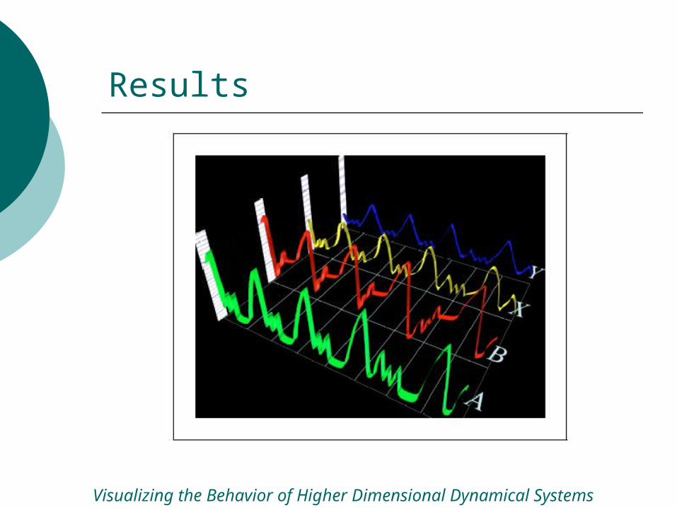
Extruded Parallel Coordinates
Instead of using same coordinate system for each sample, move parallel coordinate system along third spatial axis
Polylines viewed as cross sections of a moving plane with a complex surface that defines the trajectory
Visualizing the Behavior of Higher Dimensional Dynamical Systems

Extruded Parallel Coordinates
Visualizing the Behavior of Higher Dimensional Dynamical Systems

Extruded Parallel Coordinates
Geometry of surface can be generated and modified quickly
Clustering and correlation visually detectable
Convergence and divergence pbserved by varying the starting coordinates of the trajectory slightly
Visualizing the Behavior of Higher Dimensional Dynamical Systems
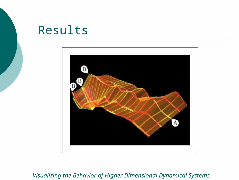
Linking with Wings
Two dimensions of high-dimensional system selected and displayed as a two-dimensional trajectory within a base plane
Third dimension of display can now be use to display third variable over base trajectory
If resulting three-dimensional trajectory is connected with base trajectory, thought of as a wing on the base trajectory Wing can be tilted at each point within a plane
normal to base trajectory
Visualizing the Behavior of Higher Dimensional Dynamical Systems

Linking with Wings
Visualizing the Behavior of Higher Dimensional Dynamical Systems
Linking with Wings
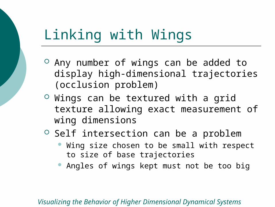
Any number of wings can be added to display high-dimensional trajectories (occlusion problem)
Wings can be textured with a grid texture allowing exact measurement of wing dimensions
Self intersection can be a problem Wing size chosen to be small with respect to size
of base trajectories Angles of wings kept must not be too big
Visualizing the Behavior of Higher Dimensional Dynamical Systems
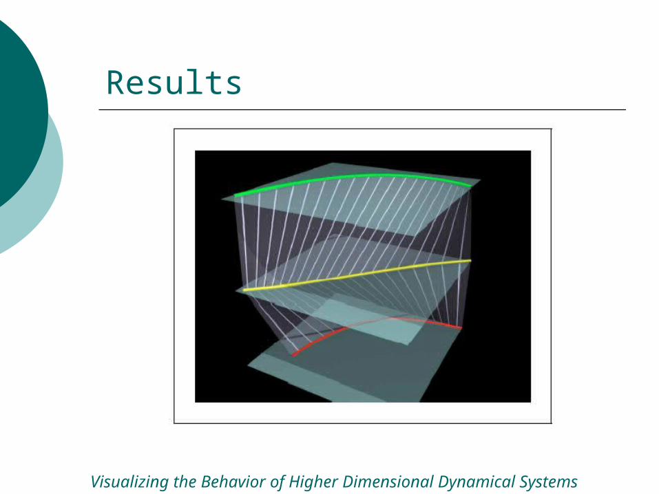
Three-dimensional Parallel Coordinates
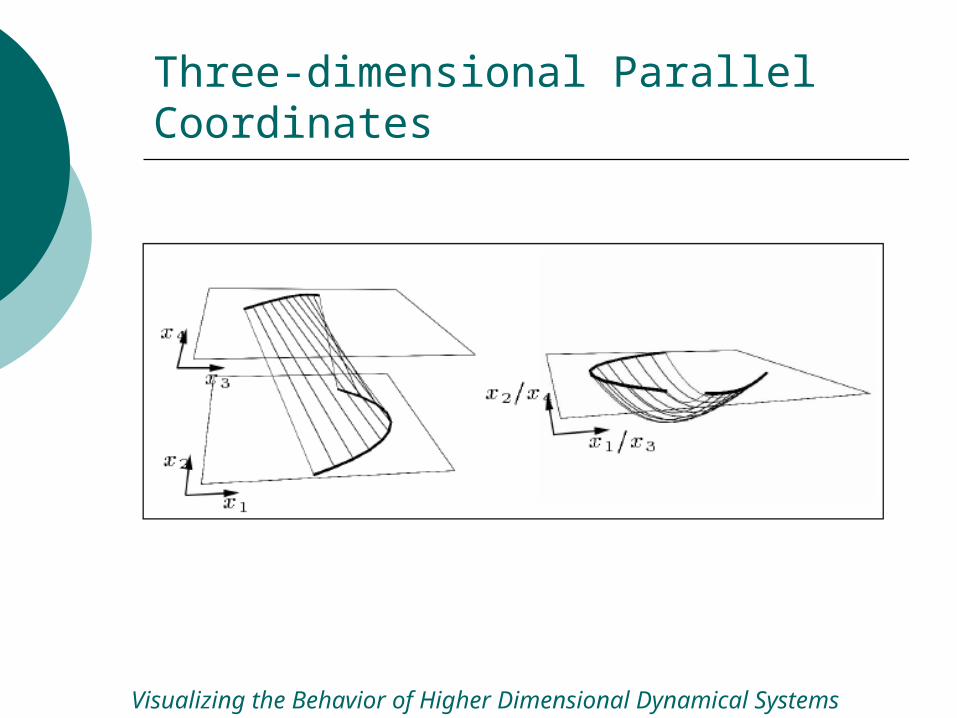
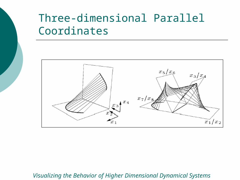
Based on parallel coordinate method One-dimensional spaces put together within
two-dimensional space (planes) and linked with polylines
Positioning of planes is more flexible Can be moved, rotated within three-dimensional
space
Visualizing the Behavior of Higher Dimensional Dynamical Systems
Three-dimensional Parallel Coordinates
Visualizing the Behavior of Higher Dimensional Dynamical Systems
Three-dimensional Parallel Coordinates
Visualizing the Behavior of Higher Dimensional Dynamical Systems
Results
Visualizing the Behavior of Higher Dimensional Dynamical Systems
Results
Visualizing the Behavior of Higher Dimensional Dynamical Systems

Results
Visualizing the Behavior of Higher Dimensional Dynamical Systems
Results
Visualizing the Behavior of Higher Dimensional Dynamical Systems

Results
Visualizing the Behavior of Higher Dimensional Dynamical Systems
Problem Addressed
Large multivariate can be difficult to navigate
Need a low dimensional representation to easy navigation
Metric scaling used as basis for creating low-dimensional overview
Multivariate Visualization Using Metric Scaling
Metric Scaling
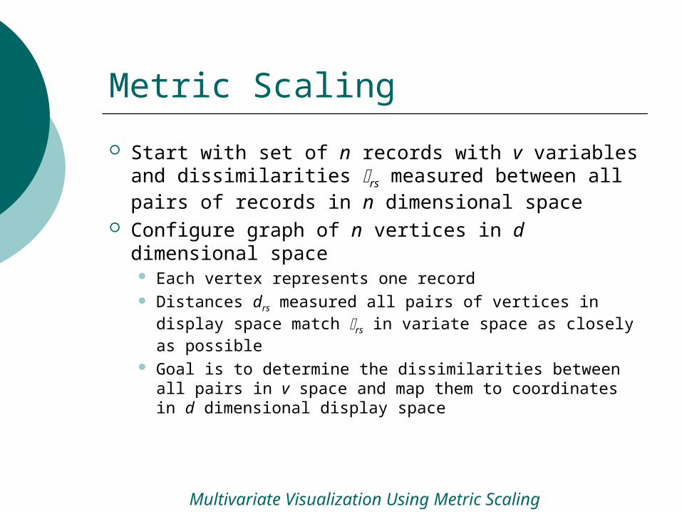
Start with set of n records with v variables and dissimilarities rs measured between all pairs of records in n dimensional space
Configure graph of n vertices in d dimensional space Each vertex represents one record Distances drs measured all pairs of vertices in display
space match rs in variate space as closely as possible
Goal is to determine the dissimilarities between all pairs in v space and map them to coordinates in d dimensional display space
Multivariate Visualization Using Metric Scaling

Metric Scaling
Multivariate Visualization Using Metric Scaling
Data Dissimilarity Measurement
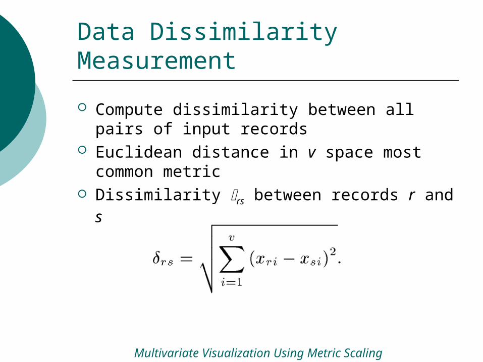
Compute dissimilarity between all pairs of input records
Euclidean distance in v space most common metric
Dissimilarity rs between records r and s
Multivariate Visualization Using Metric Scaling
Data Dissimilarity Measurement
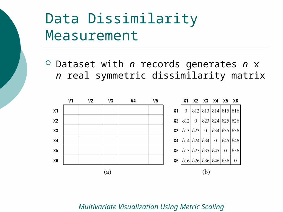
Dataset with n records generates n x n real symmetric dissimilarity matrix
Multivariate Visualization Using Metric Scaling

Recovery of Coordinates
Represent data as points in new p dimensional space where p <= n
Create inner product matrix from rs in variate space, find its non-negative eigenvalues and the corresponding eigenvectors Yield the Euclidean coordinates of n vertices in p
dimensional space
Multivariate Visualization Using Metric Scaling
Principal Coordinates
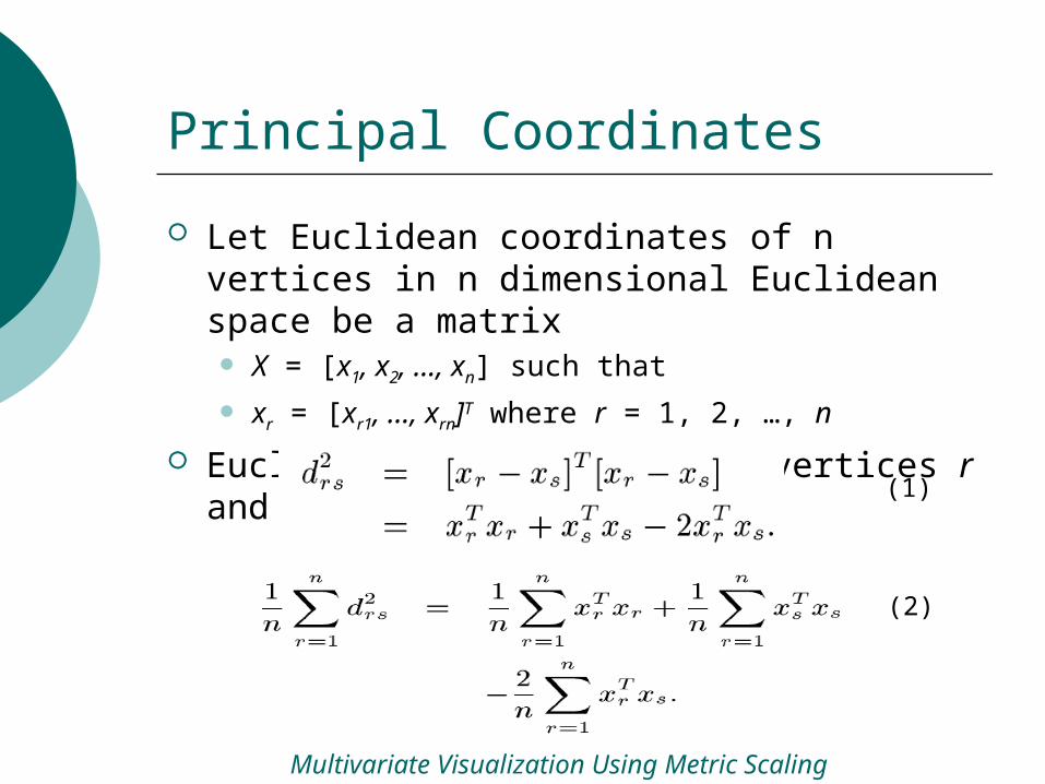
Let Euclidean coordinates of n vertices in n dimensional Euclidean space be a matrix X = [x1, x2, …, xn] such that
xr = [xr1, …, xrn]T where r = 1, 2, …, n
Euclidean distance between vertices r and s
Multivariate Visualization Using Metric Scaling
(1)
(2)

Principal Coordinates
Standardize data to have zero mean and unit variance, center of mass of the vertices is the origin
Multivariate Visualization Using Metric Scaling

Principal Coordinates
Multivariate Visualization Using Metric Scaling
since
Equation (2) becomes
(3)

Principal Coordinates
Similarly
(4)
Multivariate Visualization Using Metric Scaling
Principal Coordinates
Multivariate Visualization Using Metric Scaling
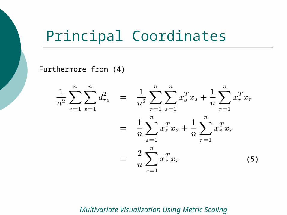
Furthermore from (4)
(5)
Principal Coordinates
Multivariate Visualization Using Metric Scaling
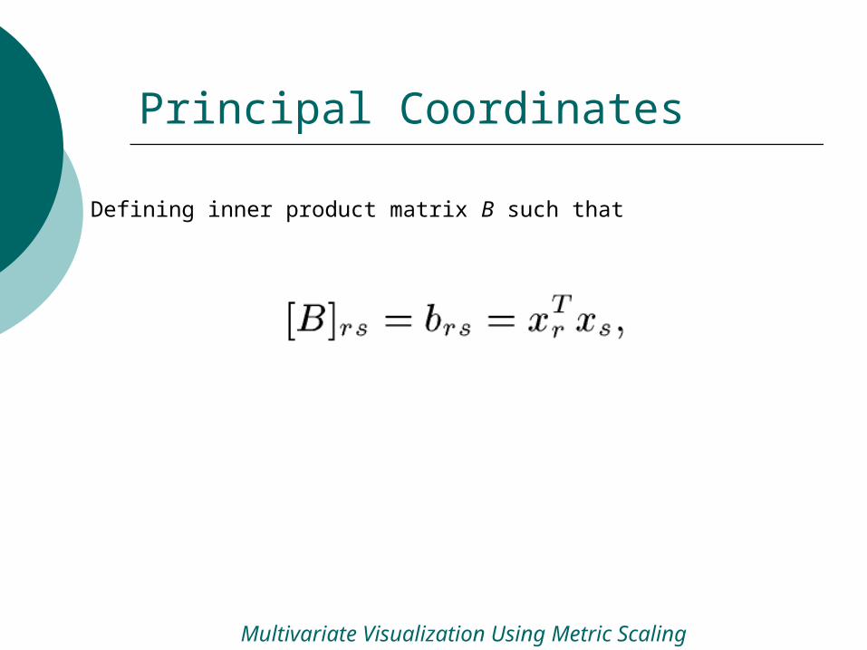
Defining inner product matrix B such that
Principal Coordinates
Multivariate Visualization Using Metric Scaling
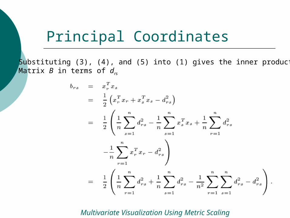
Substituting (3), (4), and (5) into (1) gives the inner productMatrix B in terms of drs
Principal Coordinates
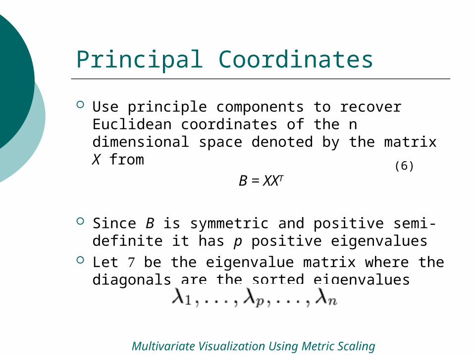
Use principle components to recover Euclidean coordinates of the n dimensional space denoted by the matrix X from
B = XXT
Since B is symmetric and positive semi-definite it has p positive eigenvalues
Let be the eigenvalue matrix where the diagonals are the sorted eigenvalues
Multivariate Visualization Using Metric Scaling
(6)
Principal Coordinates
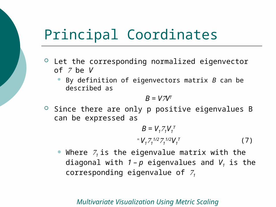
Let the corresponding normalized eigenvector of be V By definition of eigenvectors matrix B can be described
as
B = VVT
Since there are only p positive eigenvalues B can be expressed as
B = V11V1T
= V111/21
1/2V1T
Where 1 is the eigenvalue matrix with the diagonal with 1 – p eigenvalues and V1 is the corresponding eigenvalue of 1
Multivariate Visualization Using Metric Scaling
(7)
Principal Coordinates
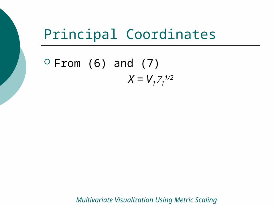
From (6) and (7)X = V11
1/2
Multivariate Visualization Using Metric Scaling

Recovery of Coordinates
If eigenvalues are sorted in desending order the first principal component associated with the first eigenvalue is more important than the second
The distance between vertices r and s is
Where xr and xs are the distance vectors associated with points r and s respectively
Multivariate Visualization Using Metric Scaling
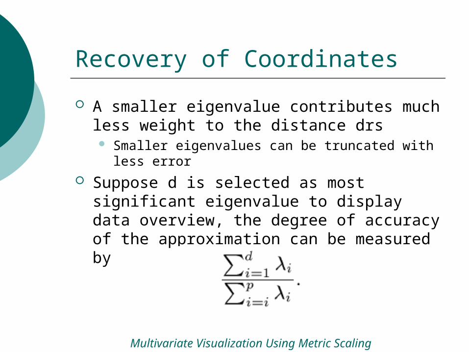
Recovery of Coordinates
A smaller eigenvalue contributes much less weight to the distance drs Smaller eigenvalues can be truncated with less
error Suppose d is selected as most significant
eigenvalue to display data overview, the degree of accuracy of the approximation can be measured by
Multivariate Visualization Using Metric Scaling
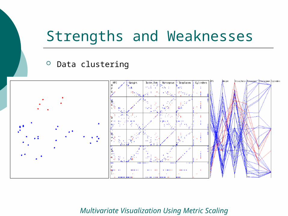
Strengths and Weaknesses
Data clustering
Multivariate Visualization Using Metric Scaling

Strengths and Weaknesses
Display Density
Multivariate Visualization Using Metric Scaling
Strengths and Weaknesses
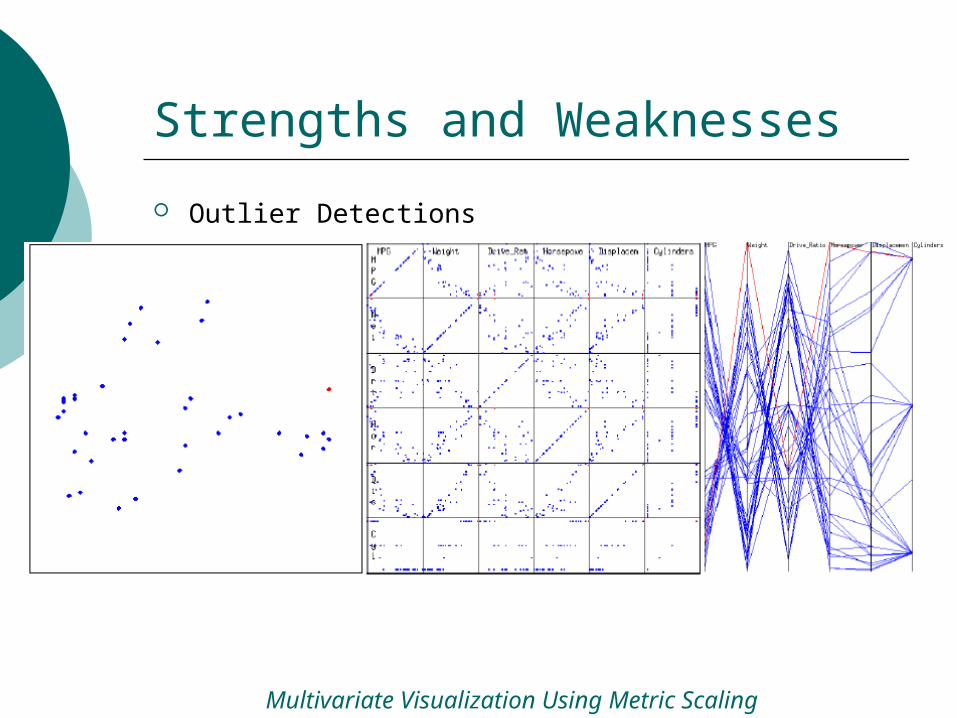
Outlier Detections
Multivariate Visualization Using Metric Scaling
Strengths and Weaknesses
Multiresolution Visualization Prograssive refinement to visualize datasets with
many variates
Multivariate Visualization Using Metric Scaling

Strengths and Weaknesses
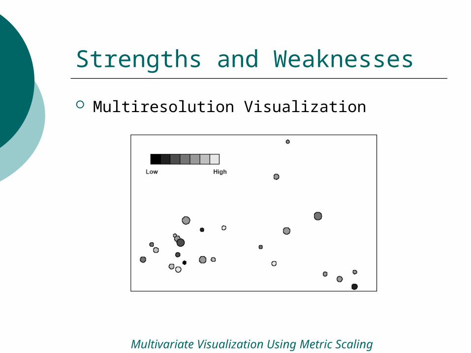
Multiresolution Visualization
Multivariate Visualization Using Metric Scaling

Strengths and Weaknesses
Multiresolution Visualization
Multivariate Visualization Using Metric Scaling
Strengths and Weaknesses
Multiresolution Visualization
Multivariate Visualization Using Metric Scaling

Strengths and Weaknesses
Individual variate values are lost
Multivariate Visualization Using Metric Scaling

Integration of Techniques
Linking
Multivariate Visualization Using Metric Scaling
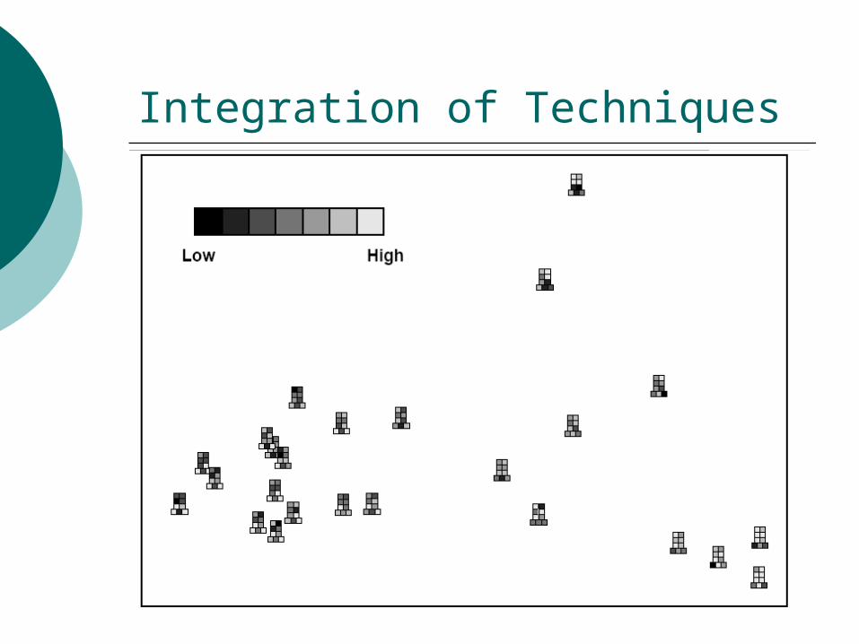
Integration of Techniques
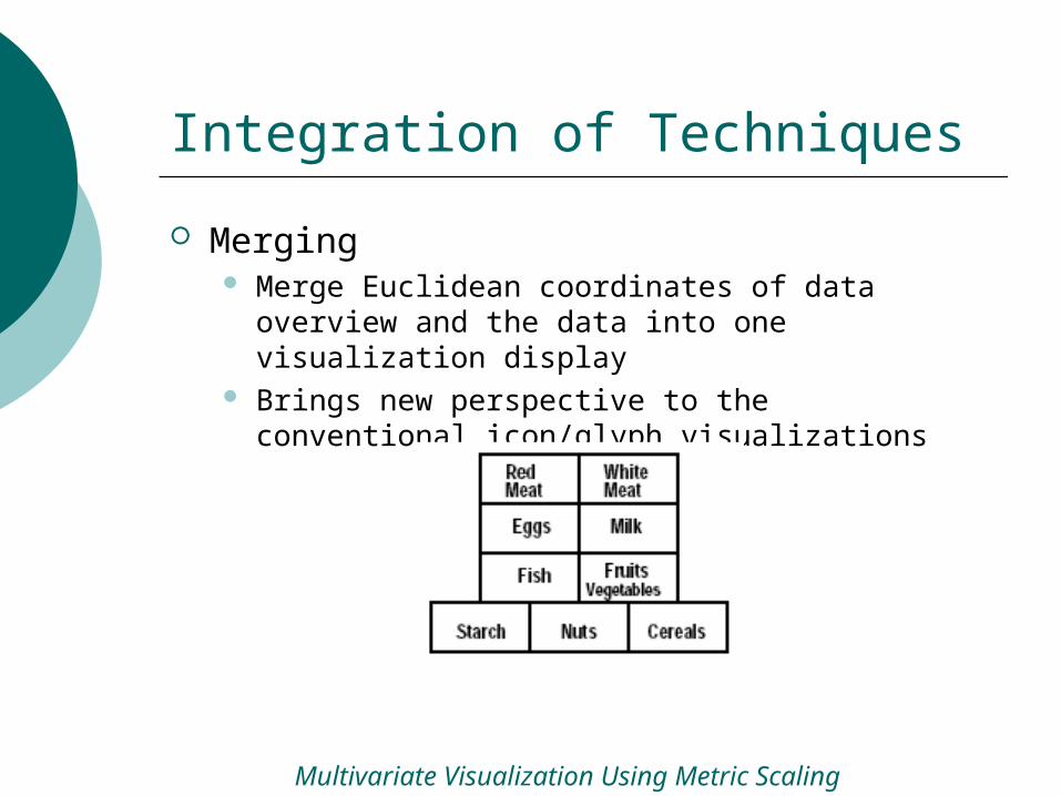
Merging Merge Euclidean coordinates of data overview
and the data into one visualization display Brings new perspective to the conventional
icon/glyph visualizations
Multivariate Visualization Using Metric Scaling
Integration of Techniques
Questions?