A highly efficient semismooth Newton augmented Lagrangian

method for solving Lasso problems∗

Xudong Li†, Defeng Sun‡ and Kim-Chuan Toh§

April 27, 2017

Abstract

We develop a fast and robust algorithm for solving large scale convex composite optimizationmodels with an emphasis on the `1-regularized least squares regression (Lasso) problems. Despitethe fact that there exist a large number of solvers in the literature for the Lasso problems, wefound that no solver can efficiently handle difficult large scale regression problems with realdata. By leveraging on available error bound results to realize the asymptotic superlinearconvergence property of the augmented Lagrangian algorithm, and by exploiting the secondorder sparsity of the problem through the semismooth Newton method, we are able to proposean algorithm, called Ssnal, to efficiently solve the aforementioned difficult problems. Undervery mild conditions, which hold automatically for Lasso problems, both the primal and the dualiteration sequences generated by Ssnal possess a fast linear convergence rate, which can evenbe superlinear asymptotically. Numerical comparisons between our approach and a number ofstate-of-the-art solvers, on real data sets, are presented to demonstrate the high efficiency androbustness of our proposed algorithm in solving difficult large scale Lasso problems.

Keywords: Lasso, sparse optimization, augmented Lagrangian, metric subregularity, semismooth-ness, Newton’s method

AMS subject classifications: 65F10, 90C06, 90C25, 90C31

1 Introduction

In this paper, we aim to design a highly efficient and robust algorithm for solving convex compositeoptimization problems including the following `1-regularized least squares (LS) problem

min

1

2‖Ax− b‖2 + λ‖x‖1

, (1)

∗An earlier version of this paper was made available in arXiv as arXiv:1607.05428. This research is supported inpart by the Ministry of Education, Singapore, Academic Research Fund under Grant R-146-000-194-112.†Department of Mathematics, National University of Singapore, 10 Lower Kent Ridge Road, Singapore

(matlixu@nus.edu.sg).‡Department of Mathematics and Risk Management Institute, National University of Singapore, 10 Lower Kent

Ridge Road, Singapore (matsundf@nus.edu.sg).§Department of Mathematics, National University of Singapore, 10 Lower Kent Ridge Road, Singapore

(mattohkc@nus.edu.sg).

1

where A : X → Y is a linear map whose adjoint is denoted as A∗, b ∈ Y and λ > 0 are given data,and X , Y are two real finite dimensional Euclidean spaces each equipped with an inner product〈·, ·〉 and its induced norm ‖ · ‖.

With the advent of convenient automated data collection technologies, the Big Data era bringsnew challenges in analyzing massive data due to the inherent sizes – large samples and high di-mensionality [15]. In order to respond to these challenges, researchers have developed many newstatistical tools to analyze such data. Among these, the `1-regularized models are arguably themost intensively studied. They are used in many applications, such as in compressive sensing,high-dimensional variable selection and image reconstruction, etc. Most notably, the model (1),named as Lasso, was proposed in [48] and has been used heavily in high-dimensional statistics andmachine learning. The model (1) has also been studied in the signal processing context under thename of basis pursuit denoising [9]. In addition to its own importance in statistics and machinelearning, Lasso problem (1) also appears as an inner subproblem of many important algorithms.For example, in recent papers [4, 1], a level set method was proposed to solve a computationallymore challenging reformulation of the Lasso problem, i.e.,

min

‖x‖1 |

1

2‖Ax− b‖2 ≤ σ

.

The level set method relies critically on the assumption that the following optimization problem,the same type as (1),

min

1

2‖Ax− b‖2 + δBλ(x)

, Bλ = x | ‖ · ‖1 ≤ λ,

can be efficiently solved to high accuracy. The Lasso-type optimization problems also appearas subproblems in various proximal Newton methods for solving convex composite optimizationproblems [7, 29, 53]. Notably, in a broader sense, all these proximal Newton methods belong to theclass of algorithms studied in [17].

The above mentioned importance together with a wide range of applications of (1) has in-spired many researchers to develop various algorithms for solving this problem and its equivalentreformulations. These algorithms can roughly be divided into two categories. The first categoryconsists of algorithms that use only the gradient information, for example, accelerated proximalgradient (APG) method [37, 2], GPSR [16], SPGL1 [4], SpaRSA [50], FPC AS [49], and NESTA[3], to name only a few. Meanwhile, algorithms in the second category, including but not limitedto mfIPM [18], SNF [36], BAS [6], SQA [7], OBA [26], FBS-Newton [51], utilize the second orderinformation of the underlying problem in the algorithmic design to accelerate the convergence. N-early all of these second order information based solvers rely on certain nondegeneracy assumptionsto guarantee the non-singularity of the corresponding inner linear systems. The only exception isthe inexact interior-point-algorithm based solver mfIPM, which does not rely on the nondegeneracyassumption but require the availability of appropriate pre-conditioners to ameliorate the extremeill-conditioning in the linear systems of the subproblems. For nondegenerate problems, the solversin the second category generally work quite well and usually outperform the algorithms in the firstcategory when high accuracy solutions are sought. In this paper, we also aim to solve the Lassoproblems by making use of the second order information. The novelty of our approach is that we donot need any nondegeneracy assumption in our theory or computations. The core idea is to analyzethe fundamental nonsmooth structures in the problems to formulate and solve specific semismooth

2

equations with well conditioned symmetric and positive definite generalized Jacobian matrices,which consequently play a critical role in our algorithmic design. When applied to solve difficultlarge scale sparse optimization problems, even for degenerate ones, our approach can outperformthe first order algorithms by a huge margin regardless of whether low or high accuracy solutionsare sought. This is in a sharp contrast to most of the other second order based solvers mentionedabove, where their competitive advantages over first-order methods only become apparent whenhigh accuracy solutions are sought.

Our proposed algorithm is a semismooth Newton augmented Lagrangian method (in short,Ssnal) for solving the dual of problem (1) where the sparsity property of the second order gener-alized Hessian is wisely exploited. This algorithmic framework is adapted from those appeared in[54, 25, 52, 31] for solving semidefinite programming problems where impressive numerical resultshave been reported. Specialized to the vector case, our Ssnal possesses unique features that arenot available in the semidefinite programming case. It is these combined unique features that allowour algorithm to converge at a very fast speed with very low computational costs at each step.Indeed, for large scale sparse Lasso problems, our numerical experiments show that the proposedalgorithm needs at most a few dozens of outer iterations to reach solutions with the desired accura-cy while all the inner semismooth Newton subproblems can be solved very cheaply. One reason forthis impressive performance is that the piecewise linear-quadratic structure of the Lasso problem(1) guarantees the asymptotic superlinear convergence of the augmented Lagrangian algorithm.Beyond the piecewise linear-quadratic case, we also study more general functions to guarantee thisfast convergence rate. More importantly, since there are several desirable properties including thestrong convexity of the objective function in the inner subproblems, in each outer iteration weonly need to execute a few (usually one to four) semismooth Newton steps to solve the underlyingsubproblem. As will be shown later, for Lasso problems with sparse optimal solutions, the compu-tational costs of performing these semismooth Newton steps can be made to be extremely cheapcompared to other costs. This seems to be counter-intuitive as normally one would expect a secondorder method to be computationally much more expensive than the first order methods at eachstep. Here, we make this counter-intuitive achievement possible by carefully exploiting the secondorder sparsity in the augmented Lagrangian functions. Notably, our algorithmic framework not on-ly works for models such as Lasso, adaptive Lasso [56] and elastic net [57], but can also be appliedto more general convex composite optimization problems. The high performance of our algorithmalso serves to show that the second order information, more specifically the nonsmooth secondorder information, can be and should be incorporated intelligently into the algorithmic design forlarge scale optimization problems.

The remaining parts of this paper are organized as follows. In the next section, we introducesome definitions and present preliminary results on the metric subregularity of multivalued map-pings. We should emphasize here that these stability results play a pivotal role in the analysis of theconvergence rate of our algorithm. In Section 3, we propose an augmented Lagrangian algorithmto solve the general convex composite optimization model and analyze its asymptotic superlinearconvergence. The semismooth Newton algorithm for solving the inner subproblems and the effi-cient implementation of the algorithm are also presented in this section. In Section 4, we conductextensive numerical experiments to evaluate the performance of Ssnal in solving various Lassoproblems. We conclude our paper in the final section.

3

2 Preliminaries

We discuss in this section some stability properties of convex composite optimization problems. Itwill become apparent later that these stability properties are the key ingredients for establishingthe fast convergence of our augmented Lagrangian method.

Recall that X and Y are two real finite dimensional Euclidean spaces. For a given closed properconvex function p : X → (−∞,+∞], the proximal mapping Proxp(·) associated with p is definedby

Proxp(x) := arg minu∈X

p(x) +

1

2‖u− x‖2

, ∀x ∈ X .

We will often make use of the following Moreau identity Proxtp(x) + tProxp∗/t(x/t) = x, wheret > 0 is a given parameter. Denote dist(x,C) = infx′∈C ‖x−x′‖ for any x ∈ X and any set C ⊂ X .

Let F : X ⇒ Y be a multivalued mapping. We define the graph of F to be the set

gphF := (x, y) ∈ X × Y | y ∈ F (x).

F−1, the inverse of F , is the multivalued mapping from Y to X whose graph is (y, x) | (x, y) ∈gphF.

Definition 1 (Error bound). Let F : X ⇒ Y be a multivalued mapping and y ∈ Y satisfy F−1(y) 6=∅. F is said to satisfy the error bound condition for the point y with modulus κ ≥ 0, if there existsε > 0 such that if x ∈ X with dist(y, F (x)) ≤ ε then

dist(x, F−1(y)) ≤ κdist(y, F (x)). (2)

The above error bound condition was called the growth condition in [34] and was used to analyzethe local linear convergence properties of the proximal point algorithm. Recall that F : X ⇒ Yis called a polyhedral multifunction if its graph is the union of finitely many polyhedral convexsets. In [39], Robinson established the following celebrated proposition on the error bound resultfor polyhedral multifunctions.

Proposition 1. Let F be a polyhedral multifunction from X to Y. Then, F satisfies the errorbound condition (2) for any point y ∈ Y satisfying F−1(y) 6= ∅ with a common modulus κ ≥ 0.

For later uses, we present the following definition of metric subregularity from Chapter 3 in[13].

Definition 2 (Metric subregularity). Let F : X ⇒ Y be a multivalued mapping and (x, y) ∈ gphF .F is said to be metrically subregular at x for y with modulus κ ≥ 0, if there exist neighborhoods Uof x and V of y such that

dist(x, F−1(y)) ≤ κdist(y, F (x) ∩ V ), ∀x ∈ U.

From the above definition, we see that if F : X ⇒ Y satisfies the error bound condition (2) fory with the modulus κ, then it is metrically subregular at x for y with the same modulus κ for anyx ∈ F−1(y).

The following definition on essential smoothness is taken from [40, Section 26].

4

Definition 3 (Essential smoothness). A proper convex function f on X is essentially smooth if fis differentiable on int (dom f) 6= ∅ and limk→∞ ‖∇f(xk)‖ = +∞ whenever xk is a sequence inint (dom f) converging to a boundary point x of int (dom f).

In particular, a smooth convex function on X is essentially smooth. Moreover, if a closedproper convex function f is strictly convex on dom f , then its conjugate f∗ is essentially smooth[40, Theorem 26.3].

Consider the following composite convex optimization model

max−f(x) := h(Ax)− 〈c, x〉+ p(x) , (3)

where A : X → Y is a linear map, h : Y → < and p : X → (−∞,+∞] are two closed proper convexfunctions, c ∈ X is a given vector. The dual of (3) can be written as

min h∗(y) + p∗(z) | A∗y + z = c , (4)

where g∗ and p∗ are the Fenchel conjugate functions of g and h, respectively. Throughout thissection, we make the following blanket assumption on h∗(·) and p∗(·).

Assumption 1. h∗(·) is essentially smooth and p∗(·) is either an indicator function δP (·) or asupport function δ∗P (·) for some nonempty polyhedral convex set P ⊆ X . Note that ∇h∗ is locallyLipschitz continuous and directionally differentiable on int (domh∗).

Under Assumption 1, by [40, Theorem 26.1], we know that ∂h∗(y) = ∅ whenever y 6∈ int (domh∗).Denote by l the Lagrangian function for (4):

l(y, z, x) = h∗(y) + p∗(z)− 〈x, A∗y + z − c〉, ∀ (y, z, x) ∈ Y × X × X . (5)

Corresponding to the closed proper convex function f in the objective of (3) and the convex-concavefunction l in (5), define the maximal monotone operators Tf and Tl [42], by

Tf (x) := ∂f(x), Tl(y, z, x) := (y′, z′, x′) | (y′, z′,−x′) ∈ ∂l(y, z, x),

whose inverse are given, respectively, by

T −1f (x′) := ∂f∗(x′), T −1l (y′, z′, x′) := (y, z, x) | (y′, z′,−x′) ∈ ∂l(y, z, x).

Unlike the case for Tf [33, 47, 58], stability results of Tl which correspond to the perturbations ofboth primal and dual solutions are very limited. Next, as a tool for studying the convergence rateof Ssnal, we shall establish a theorem which reveals the metric subregularity of Tl under somemild assumptions.

The KKT system associated with problem (4) is given as follows:

0 ∈ ∂h∗(y)−Ax, 0 ∈ −x+ ∂p∗(z), 0 = A∗y + z − c, (x, y, z) ∈ X × Y × X .

Assume that the above KKT system has at least one solution. This existence assumption togetherwith the essentially smoothness assumption on h∗ implies that the above KKT system can beequivalently rewritten as

0 = ∇h∗(y)−Ax, 0 ∈ −x+ ∂p∗(z), 0 = A∗y + z − c, (x, y, z) ∈ X × int(domh∗)×X . (6)

5

Therefore, under the above assumptions, we only need to focus on int (domh∗) × X when solvingproblem (4). Let (y, z) be an optimal solution to problem (4). Then, we know that the set of theLagrangian multipliers associated with (y, z), denoted as M(y, z), is nonempty. Define the criticalcone associated with (4) at (y, z) as follows:

C(y, z) :=

(d1, d2) ∈ Y × X | A∗d1 + d2 = 0, 〈∇h∗(y), d1〉+ (p∗)′(z; d2) = 0, d2 ∈ Tdom(p∗)(z),(7)

where (p∗)′(z; d2) is the directional derivative of p∗ at z with respect to d2, Tdom(p∗)(z) is the tangentcone of dom(p∗) at z. When the conjugate function p∗ is taken to be the indicator function of anonempty polyhedral set P , the above definition reduces directly to the standard definition of thecritical cone in the nonlinear programming setting.

Definition 4 (Second order sufficient condition). Let (y, z) ∈ Y × X be an optimal solution toproblem (4) with M(y, z) 6= ∅. We say that the second order sufficient condition for problem (4)holds at (y, z) if

〈d1, (∇h∗)′(y; d1)〉 > 0, ∀ 0 6= (d1, d2) ∈ C(y, z).

By building on the proof ideas from the literature on nonlinear programming problems [11, 27,24], we are able to prove the following result on the metric subregularity of Tl. This allows us toprove the linear and even the asymptotic superlinear convergence of the sequences generated bythe Ssnal algorithm to be presented in the next section even when the objective in problem (3)does not possess the piecewise linear-quadratic structure as in the Lasso problem (1).

Theorem 1. Assume that the KKT system (6) has at least one solution and denote it as (x, y, z).Suppose that Assumption 1 holds and that the second order sufficient condition for problem (4)holds at (y, z). Then, Tl is metrically subregular at (y, z, x) for the origin.

Proof. First, we claim that there exists a neighborhood U of (x, y, z) such that for any w =(u1, u2, v) ∈ W := Y × X × X with ‖w‖ sufficiently small, any solution (x(w), y(w), z(w)) ∈ Uof the perturbed KKT system

0 = ∇h∗(y)−Ax− u1, 0 ∈ −x− u2 + ∂p∗(z), 0 = A∗y + z − c− v (8)

satisfies the following estimate

‖(y(w), z(w))− (y, z)‖ = O(‖w‖). (9)

For the sake of contradiction, suppose that our claim is not true. Then, there exist some sequenceswk:= (uk1, u

k2, v

k) and (xk, yk, zk) such that wk → 0, (xk, yk, zk)→ (x, y, z), for each k the point(xk, yk, zk) is a solution of (8) for w = wk, and

‖(yk, zk)− (y, z)‖ > γk‖wk‖

with some γk > 0 such that γk → ∞. Passing onto a subsequence if necessary, we assume that((yk, zk) − (y, z)

)/‖(yk, zk) − (y, z)‖ converges to some ξ = (ξ1, ξ2) ∈ Y × X , ‖ξ‖ = 1. Then,

setting tk = ‖(yk, zk) − (y, z)‖ and passing to a subsequence further if necessary, by the local

6

Lipschitz continuity and the directional differentiability of ∇h∗(·) at y, we know that for all ksufficiently large

∇h∗(yk)−∇h∗(y) =∇h∗(y + tkξ1)−∇h∗(y) +∇h∗(yk)−∇h∗(y + tkξ1)

=tk(∇h∗)′(y; ξ1) + o(tk) +O(‖yk − y − tkξ1‖)

=tk(∇h∗)′(y; ξ1) + o(tk).

Denote for each k, xk := xk + uk2. Simple calculations show that for all k sufficiently large

0 = ∇h∗(yk)−∇h∗(y)−A(xk − x) +Auk2 − uk1 = tk(∇h∗)′(y; ξ1) + o(tk)−A(xk − x) (10)

and0 = A(yk − y) + (zk − z)− vk = tk(A∗ξ1 + ξ2) + o(tk). (11)

Dividing both sides of equation (11) by tk and then taking limits, we obtain

A∗ξ1 + ξ2 = 0, (12)

which further implies that〈∇h∗(y), ξ1〉 = 〈Ax, ξ1〉 = −〈x, ξ2〉. (13)

Since xk ∈ ∂p∗(zk), we know that for all k sufficiently large,

zk = z + tkξ2 + o(tk) ∈ dom p∗.

That is, ξ2 ∈ Tdom p∗(z).According to the structure of p∗, we separate our discussions into two cases.Case I: There exists a nonempty polyhedral convex set P such that p∗(z) = δ∗P (z), ∀z ∈ X .

Then, for each k, it holds thatxk = ΠP (zk + xk).

By [14, Theorem 4.1.1], we have

xk = ΠP (zk + xk) = ΠP (z + x) + ΠC(zk − z + xk − x) = x+ ΠC(z

k − z + xk − x), (14)

where C is the critical cone of P at z + x, i.e.,

C ≡ CP (z + x) := TP (x) ∩ z⊥.

Since C is a polyhedral cone, we know from [14, Proposition 4.1.4] that ΠC(·) is a piecewise linearfunction, i.e., there exist a positive integer l and orthogonal projectors B1, . . . , Bl such that for anyx ∈ X ,

ΠC(x) ∈ B1x, . . . , Blx .

By restricting to a subsequence if necessary, we may further assume that there exists 1 ≤ j′ ≤ lsuch that for all k ≥ 1,

ΠC(zk − z + xk − x) = Bj′(z

k − z + xk − x) = ΠRange(Bj′ )(zk − z + xk − x). (15)

7

Denote L := Range(Bj′). Combining (14) and (15), we get

C ∩ L 3 (xk − x) ⊥ (zk − z) ∈ C ∩ L⊥,

where C is the polar cone of C. Since xk − x ∈ C, we have 〈xk − x, z〉 = 0, which, together with〈xk − x, zk − z〉 = 0, implies 〈xk − x, zk〉 = 0. Thus for all k sufficiently large,

〈zk, xk〉 = 〈zk, x〉 = 〈z + tkξ2 + o(tk), x〉,

and it follows that

(p∗)′(z; ξ2) = limk→∞

δ∗P (z + tkξ2)− δ∗P (z)

tk= lim

k→∞

δ∗P (zk)− δ∗P (z)

tk

= limk→∞

〈zk, xk〉 − 〈z, x〉tk

= 〈x, ξ2〉.

(16)

By (12), (13) and (16), we know that (ξ1, ξ2) ∈ C(y, z). Since C ∩ L is a polyhedral convex cone,we know from [40, Theorem 19.3] that A(C ∩ L) is also a polyhedral convex cone, which, togetherwith (10), implies

(∇h∗)′(y; ξ1) ∈ A(C ∩ L).

Therefore, there exists a vector η ∈ C ∩ L such that

〈ξ1, (∇h∗)′(y; ξ1)〉 = 〈ξ1, Aη〉 = −〈ξ2, η〉 = 0,

where the last equality follows from the fact that ξ2 ∈ C ∩ L⊥. Note that the last inclusion holdssince the polyhedral convex cone C ∩ L⊥ is closed and

ξ2 = limk→∞

zk − ztk

∈ C ∩ L⊥.

As 0 6= ξ = (ξ1, ξ2) ∈ C(y, z), but 〈ξ1, (∇h∗)′(y; ξ1)〉 = 0, this contradicts the assumption that thesecond order sufficient condition holds for (4) at (y, z). Thus we have proved our claim for Case I.

Case II: There exists a nonempty polyhedral convex set P such that p∗(z) = δP (z), ∀z ∈ X .Then, we know that for each k,

zk = ΠP (zk + xk).

Since (δP )′(z; d2) = 0,∀d2 ∈ Tdom(p∗)(z), the critical cone in (7) now takes the following form

C(y, z) =

(d1, d2) ∈ Y × X | A∗d1 + d2 = 0, 〈∇h∗(y), d1〉 = 0, d2 ∈ Tdom(p∗)(z).

Similar to Case I, without loss of generality, we can assume that there exists a subspace L suchthat for all k ≥ 1,

C ∩ L 3 (zk − z) ⊥ (xk − x) ∈ C ∩ L⊥,

whereC ≡ CP (z + x) := TP (z) ∩ x⊥.

Since C ∩ L is a polyhedral convex cone, we know

ξ2 = limk→∞

zk − ztk

∈ C ∩ L,

8

and consequently 〈ξ2, x〉 = 0, which, together with (12) and (13), implies ξ = (ξ1, ξ2) ∈ C(y, z). By(10) and the fact that A(C ∩ L⊥) is a polyhedral convex cone, we know that

(∇h∗)′(y; ξ1) ∈ A(C ∩ L⊥).

Therefore, there exists a vector η ∈ C ∩ L⊥ such that

〈ξ1, (∇h∗)′(y; ξ1)〉 = 〈ξ1, Aη〉 = −〈ξ2, η〉 = 0.

Since ξ = (ξ1, ξ2) 6= 0, we arrive at a contradiction to the assumed second order sufficient condition.So our claim is also true for this case.

In summary, we have proven that there exists a neighborhood U of (x, y, z) such that for anyw close enough to the origin, equation (9) holds for any solution (x(w), y(w), z(w)) ∈ U to theperturbed KKT system (8). Next we show that Tl is metrically subregular at (y, z, x) for theorigin.

Define the mapping ΘKKT : X × Y × X ×W → Y ×X × X by

ΘKKT (x, y, z, w) :=

∇h∗(y)−Ax− u1z − Proxp∗(z + x+ u2)A∗y + z − c− v

, ∀(x, y, z, w) ∈ X × Y × X ×W

and define the mapping θ : X → Y × X × X as follows:

θ(x) := ΘKKT(x, y, z, 0), ∀x ∈ X .

Then, we have x ∈ M(y, z) if and only if θ(x) = 0. Since Proxp∗(·) is a piecewise affine function,θ(·) is a piecewise affine function and thus a polyhedral multifunction. By using Proposition 1 andshrinking the neighborhood U if necessary, for any w close enough to the origin and any solution(x(w), y(w), z(w)) ∈ U of the perturbed KKT system (8), we have

dist(x(w),M(y, z)) = O(‖θ(x(w))‖)

= O(‖ΘKKT(x(w), y, z, 0)−ΘKKT(x(w), y(w), z(w), w)‖)

= O(‖w‖+ ‖(y(w), z(w))− (y, z)‖),

which, together with (9), implies the existence of a constant κ ≥ 0 such that

‖(y(w), z(w))− (y, z)‖+ dist(x(w),M(y, z)) ≤ κ‖w‖. (17)

Thus, by Definition 2, we have proven that Tl is metrically subregular at (y, z, x) for the origin.The proof of the theorem is completed.

Remark 1. For convex piecewise linear-quadratic programming problems such as the `1 and elasticnet regularized LS problem, we know from [46] and [43, Proposition 12.30] that the correspondingoperators Tl and Tf are polyhedral multifunctions and thus, by Proposition 1, the error boundcondition holds. Here we emphasize again that the error bound condition holds for the Lasso problem(1). Moreover, Tf , associated with the `1 or elastic net regularized logistic regression model, i.e.,for a given vector b ∈ <m, the loss function h : <m → < in problem (3) takes the form

h(y) =

m∑i=1

log(1 + e−biyi), ∀y ∈ <m,

9

also satisfies the error bound condition [33, 47]. Meanwhile, from Theorem 1, we know that Tlcorresponding to the `1 or the elastic net regularized logistic regression model is metrically subregularat any solutions to the KKT system (6) for the origin.

3 An augmented Lagrangian method with asymptotic superlinearconvergence

Recall the general convex composite model (3)

(P) max−f(x) = h(Ax)− 〈c, x〉+ p(x)

and its dual(D) minh∗(y) + p∗(z) | A∗y + z = c.

In this section, we shall propose an asymptotically superlinearly convergent augmented Lagrangianmethod for solving (P) and (D). In this section, we make the following standing assumptionsregarding the function h.

Assumption 2. (a) h : Y → < is a convex differentiable function whose gradient is 1/αh-Lipschitz continuous, i.e.,

‖∇h(y′)−∇h(y)‖ ≤ (1/αh)‖y′ − y‖, ∀y′, y ∈ Y.

(b) h is essentially locally strongly convex [21], i.e., for any compact and convex set K ⊂ dom ∂h,there exists βK > 0 such that

(1− λ)h(y′) + λh(y) ≥ h((1− λ)y′ + λy) +1

2βKλ(1− λ)‖y′ − y‖2, ∀y′, y ∈ K,

for all λ ∈ [0, 1].

Many commonly used loss functions in the machine learning literature satisfy the above mildassumptions. For example, h can be the loss function in the linear regression, logistic regressionand Poisson regression models. While the strict convexity of a convex function is closely relatedto the differentiability of its conjugate, the essential local strong convexity in Assumption 2(b)for a convex function was first proposed in [21] to obtain a characterization of the local Lipschitzcontinuity of the gradient of its conjugate function.

The aforementioned assumptions on h imply the following useful properties of h∗. Firstly, by[43, Proposition 12.60], we know that h∗ is strongly convex with modulus αh. Secondly, by [21,Corollary 4.4], we know that h∗ is essentially smooth and ∇h∗ is locally Lipschitz continuous onint (domh∗). If the solution set to the KKT system associated with (P) and (D) is further assumedto be nonempty, similar to what we have discussed in the last section, one only needs to focus onint (domh∗) × X when solving (D). Given σ > 0, the augmented Lagrangian function associatedwith (D) is given by

Lσ(y, z;x) := l(y, z, x) +σ

2‖A∗y + z − c‖2, ∀ (y, z, x) ∈ Y × X × X ,

where the Lagrangian function l(·) is defined in (5).

10

3.1 Ssnal: A semismooth Newton augmented Lagrangian algorithm for (D)

The detailed steps of our algorithm Ssnal for solving (D) are given as follows. Since a semismoothNewton method will be employed to solve the subproblems involved in this prototype of the inexactaugmented Lagrangian method [42], it is natural for us to call our algorithm as Ssnal.

Algorithm Ssnal: An inexact augmented Lagrangian method for (D).

Let σ0 > 0 be a given parameter. Choose (y0, z0, x0) ∈ int(domh∗)× dom p∗×X . For k = 0, 1, . . .,perform the following steps in each iteration:

Step 1. Compute(yk+1, zk+1) ≈ arg minΨk(y, z) := Lσk(y, z;xk). (18)

Step 2. Compute xk+1 = xk − σk(A∗yk+1 + zk+1 − c) and update σk+1 ↑ σ∞ ≤ ∞ .

Next, we shall adapt the results developed in [41, 42] and [34] to establish the global and localsuperlinear convergence of our algorithm.

Since the inner problems can not be solved exactly, we use the following standard stoppingcriterion studied in [41, 42] for approximately solving (18)

(A) Ψk(yk+1, zk+1)− inf Ψk ≤ ε2k/2σk,

∞∑k=0

εk <∞.

Now, we can state the global convergence of Algorithm Ssnal from [41, 42] without much difficulty.

Theorem 2. Suppose that Assumption 2 holds and that the solution set to (P) is nonempty. Let(yk, zk, xk) be the infinite sequence generated by Algorithm Ssnal with stopping criterion (A).Then, the sequence xk is bounded and converges to an optimal solution of (P). In addition,(yk, zk) is also bounded and converges to the unique optimal solution (y∗, z∗) ∈ int(domh∗) ×dom p∗ of (D).

Proof. Since the solution set to (P) is assumed to be nonempty, the optimal value of (P) is finite.From Assumption 2(a), we have that domh = Y and h∗ is strongly convex [43, Proposition 12.60].Then, by Fenchel’s Duality Theorem [40, Corollary 31.2.1], we know that the solution set to (D) isnonempty and the optimal value of (D) is finite and equals to the optimal value of (P). That is, thesolution set to the KKT system associated with (P) and (D) is nonempty. The uniqueness of theoptimal solution (y∗, z∗) ∈ int(domh∗)× X of (D) then follows directly from the strong convexityof h∗. By combining this uniqueness with [42, Theorem 4], one can easily obtain the boundednessof (yk, zk) and other desired results readily.

We need the the following stopping criteria for the local convergence analysis:

(B1) Ψk(yk+1, zk+1)− inf Ψk ≤ (δ2k/2σk)‖xk+1 − xk‖2,

∞∑k=0

δk < +∞,

(B2) dist(0, ∂Ψk(yk+1, zk+1)) ≤ (δ′k/σk)‖xk+1 − xk‖, 0 ≤ δ′k → 0.

where xk+1 := xk + σk(A∗yk+1 + zk+1 − c).

11

Theorem 3. Assume that Assumption 2 holds and that the solution set Ω to (P) is nonemp-ty. Suppose that Tf satisfies the error bound condition (2) for the origin with modulus af . Let(yk, zk, xk) be any infinite sequence generated by Algorithm Ssnal with stopping criteria (A) and(B1). Then, the sequence xk converges to x∗ ∈ Ω and for all k sufficiently large,

dist(xk+1,Ω) ≤ θkdist(xk,Ω), (19)

where θk =(af (a2f +σ2k)

−1/2+2δk)(1−δk)−1 → θ∞ = af (a2f +σ2∞)−1/2 < 1 as k → +∞. Moreover,

the sequence (yk, zk) converges to the optimal unique solution (y∗, z∗) ∈ int(domh∗)× dom p∗ to(D).

Moreover, if Tl is metrically subregular at (y∗, z∗, x∗) for the origin with modulus al and thestopping criterion (B2) is also used, then for all k sufficiently large,

‖(yk+1, zk+1)− (y∗, z∗)‖ ≤ θ′k‖xk+1 − xk‖,

where θ′k = al(1 + δ′k)/σk with limk→∞ θ′k = al/σ∞.

Proof. The first part of the theorem follows from [34, Theorem 2.1], [42, Proposition 7, Theorem 5]and Theorem 2. To prove the second part, we recall that if Tl is metrically subregular at (y∗, z∗, x∗)for the origin with the modulus al and (yk, zk, xk)→ (y∗, z∗, x∗), then for all k sufficiently large,

‖(yk+1, zk+1)− (y∗, z∗)‖+ dist(xk+1,Ω) ≤ al dist(0, Tl(yk+1, zk+1, xk+1)).

Therefore, by the estimate (4.21) in [42] and the stopping criterion (B2), we obtain that for all ksufficiently large,

‖(yk+1, zk+1)− (y∗, z∗)‖ ≤ al(1 + δ′k)/σk‖xk+1 − xk‖.

This completes the proof for Theorem 3.

Remark 2. Recently advances in [12] reveal the asymptotic R-superliner convergence of the dualiteration sequence (yk, zk). Indeed, from [12, Proposition 4.1], under the same conditions ofTheorem 3, we have that for k sufficiently large,

‖(yk+1, zk+1)− (y∗, z∗)‖ ≤ θ′k‖xk+1 − xk‖ ≤ θ′k(1− δk)−1dist(xk, Ω), (20)

where θ′k(1 − δk)−1 → al/σ∞. Then, if σ∞ = ∞, inequalities (19) and (20) imply that xk and(yk, zk) converge Q-superlinearly and R-superlinearly, respectively.

We should emphasize here that by combining Remarks 1 and 2 and Theorem 3, our AlgorithmSsnal is guaranteed to produce an asymptotically superlinearly convergent sequence when usedto solve (D) for many commonly used regularizers and loss functions. In particular, the Ssnalalgorithm is asymptotically superlinearly convergent when applied to the dual of (1).

3.2 Solving the augmented Lagrangian subproblems

Here we shall propose an efficient semismooth Newton algorithm to solve the inner subproblems inthe augmented Lagrangian method (18). That is, for some fixed σ > 0 and x ∈ X , we consider tosolve

miny,z

Ψ(y, z) := Lσ(y, z; x). (21)

12

Since Ψ(·, ·) is a strongly convex function, we have that, for any α ∈ <, the level set Lα := (y, z) ∈domh∗ × dom p∗ | Ψ(y, z) ≤ α is a closed and bounded convex set. Moreover, problem (21)admits a unique optimal solution denoted as (y, z) ∈ int(domh∗)× dom p∗.

Denote, for any y ∈ Y,

ψ(y) := infz

Ψ(y, z)

= h∗(y) + p∗(Proxp∗/σ(x/σ −A∗y + c)) +1

2σ‖Proxσp(x− σ(A∗y − c))‖2 − 1

2σ‖x‖2.

Therefore, if (y, z) = arg min Ψ(y, z), then (y, z) ∈ int(domh∗)× dom p∗ can be computed simulta-neously by

y = arg minψ(y), z = Proxp∗/σ(x/σ −A∗y + c).

Note that ψ(·) is strongly convex and continuously differentiable on int(domh∗) with

∇ψ(y) = ∇h∗(y)−AProxσp(x− σ(A∗y − c)), ∀y ∈ int(domh∗).

Thus, y can be obtained via solving the following nonsmooth equation

∇ψ(y) = 0, y ∈ int(domh∗). (22)

Let y ∈ int(domh∗) be any given point. Since h∗ is a convex function with a locally Lipschitzcontinuous gradient on int(domh∗), the following operator is well defined:

∂2ψ(y) := ∂(∇h∗)(y) + σA∂Proxσp(x− σ(A∗y − c))A∗,

where ∂(∇h∗)(y) is the Clarke subdifferential of ∇h∗ at y [10], and ∂Proxσp(x− σ(A∗y− c)) is theClarke subdifferential of the Lipschitz continuous mapping Proxσp(·) at x− σ(A∗y − c). Note thatfrom [10, Proposition 2.3.3 and Theorem 2.6.6], we know that

∂2ψ(y) (d) ⊆ ∂2ψ(y) (d), ∀ d ∈ Y,

where ∂2ψ(y) denotes the generalized Hessian of ψ at y. Define

V := H + σAUA∗ (23)

with H ∈ ∂2h∗(y) and U ∈ ∂Proxσp(x − σ(A∗y − c)). Then, we have V ∈ ∂2ψ(y). Since h∗ is astrongly convex function, we know that H is symmetric positive definite on Y and thus V is alsosymmetric positive definite on Y.

Under the mild assumption that ∇h∗ and Proxσp are strongly semismooth (whose definitionis given next), we can design a superlinearly convergent semismooth Newton method to solve thenonsmooth equation (22).

Definition 5 (Semismoothness [35, 38, 45]). Let F : O ⊆ X → Y be a locally Lipschitz continuousfunction on the open set O. F is said to be semismooth at x ∈ O if F is directionally differentiableat x and for any V ∈ ∂F (x+ ∆x) with ∆x→ 0,

F (x+ ∆x)− F (x)− V∆x = o(‖∆x‖).

F is said to be strongly semismooth at x if F is semismooth at x and

F (x+ ∆x)− F (x)− V∆x = O(‖∆x‖2).

F is said to be a semismooth (respectively, strongly semismooth) function on O if it is semismooth(respectively, strongly semismooth) everywhere in O.

13

Note that it is widely known in the nonsmooth optimization/equation community that con-tinuous piecewise affine functions and twice continuously differentiable functions are all stronglysemismooth everywhere. In particular, Prox‖·‖1 , as a Lipschitz continuous piecewise affine function,is strongly semismooth. See [14] for more semismooth and strongly semismooth functions.

Now, we can design a semismooth Newton (Ssn) method to solve (22) as follows and couldexpect to get a fast superlinear or even quadratic convergence.

Algorithm Ssn: A semismooth Newton algorithm for solving (22) (Ssn(y0, x, σ)).

Given µ ∈ (0, 1/2), η ∈ (0, 1), τ ∈ (0, 1], and δ ∈ (0, 1). Choose y0 ∈ int(domh∗). Iterate thefollowing steps for j = 0, 1, . . . .

Step 1. Choose Hj ∈ ∂(∇h∗)(yj) and Uj ∈ ∂Proxσp(x − σ(A∗yj − c)). Let Vj := Hj + σAUjA∗.Solve the following linear system

Vjd+∇ψ(yj) = 0 (24)

exactly or by the conjugate gradient (CG) algorithm to find dj such that

‖Vjdj +∇ψ(yj)‖ ≤ min(η, ‖∇ψ(yj)‖1+τ ).

Step 2. (Line search) Set αj = δmj , where mj is the first nonnegative integer m for which

yj + δmdj ∈ int(domh∗) and ψ(yj + δmdj) ≤ ψ(yj) + µδm〈∇ψ(yj), dj〉.

Step 3. Set yj+1 = yj + αj dj .

The convergence results for the above Ssn algorithm are stated in the next theorem.

Theorem 4. Assume that ∇h∗(·) and Proxσp(·) are strongly semismooth on int(domh∗) and X ,respectively. Let the sequence yj be generated by Algorithm Ssn. Then yj converges to theunique optimal solution y ∈ int(domh∗) of the problem in (22) and

‖yj+1 − y‖ = O(‖yj − y‖1+τ ).

Proof. Since, by [54, Proposition 3.3], dj is a descent direction, Algorithm Ssn is well-defined. By(23), we know that for any j ≥ 0, Vj ∈ ∂2ψ(yj). Then, we can prove the conclusion of this theoremby following the proofs to [54, Theorems 3.4 and 3.5]. We omit the details here.

We shall now discuss the implementations of stopping criteria (A), (B1) and (B2) for AlgorithmSsn to solve the subproblem (18) in Algorithm Ssnal. Note that when Ssn is applied to minimizeΨk(·) to find

yk+1 = Ssn(yk, xk, σk) and zk+1 = Proxp∗/σk(xk/σk −A∗yk+1 + c),

we have, by simple calculations and the strong convexity of h∗, that

Ψk(yk+1, zk+1)− inf Ψk = ψk(y

k+1)− inf ψk ≤ (1/2αh)‖∇ψk(yk+1)‖2

14

and (∇ψk(yk+1), 0) ∈ ∂Ψk(yk+1, zk+1), where ψk(y) := infz Ψk(y, z) for all y ∈ Y. Therefore, the

stopping criteria (A), (B1) and (B2) can be achieved by the following implementable criteria

(A′) ‖∇ψk(yk+1)‖ ≤√αh/σk εk,

∑∞k=0 εk <∞,

(B1′) ‖∇ψk(yk+1)‖ ≤ √αhσk δk‖A∗yk+1 + zk+1 − c‖,∑∞

k=0 δk < +∞,

(B2′) ‖∇ψk(yk+1)‖ ≤ δ′k‖A∗yk+1 + zk+1 − c‖, 0 ≤ δ′k → 0.

That is, the stopping criteria (A), (B1) and (B2) will be satisfied as long as ‖∇ψk(yk+1)‖ is suffi-ciently small.

3.3 An efficient implementation of Ssn for solving subproblems (18)

When Algorithm Ssnal is applied to solve the general convex composite optimization model (P),the key part is to use Algorithm Ssn to solve the subproblems (18). In this subsection, we shalldiscuss an efficient implementation of Ssn for solving the aforementioned subproblems when thenonsmooth regularizer p is chosen to be λ‖ · ‖1 for some λ > 0. Clearly, in Algorithm Ssn, themost important step is the computation of the search direction dj from the linear system (24). Sowe shall first discuss the solving of this linear system.

Let (x, y) ∈ <n ×<m and σ > 0 be given. We consider the following Newton linear system

(H + σAUAT )d = −∇ψ(y), (25)

where H ∈ ∂(∇h∗)(y), A denotes the matrix representation of A with respect to the standard basesof <n and <m, U ∈ ∂Proxσλ‖·‖1(x) with x := x− σ(AT y− c). Since H is a symmetric and positivedefinite matrix, equation (25) can be equivalently rewritten as(

Im + σ(L−1A)U(L−1A)T)(LTd) = −L−1∇ψ(y),

where L is a nonsingular matrix obtained from the (sparse) Cholesky decomposition of H such thatH = LLT . In many applications, H is usually a sparse matrix. Indeed, when the function h in theprimal objective is taken to be the squared loss or the logistic loss functions, the resulting matricesH are in fact diagonal matrices. That is, the costs of computing L and its inverse are negligible inmost situations. Therefore, without loss of generality, we can consider a simplified version of (25)as follows

(Im + σAUAT )d = −∇ψ(y), (26)

which is precisely the Newton system associated with the standard Lasso problem (1). SinceU ∈ <n×n is a diagonal matrix, at the first glance, the costs of computing AUAT and the matrix-vector multiplication AUATd for a given vector d ∈ <m are O(m2n) and O(mn), respectively.These computational costs are too expensive when the dimensions of A are large and can makethe commonly employed approaches such as the Cholesky factorization and the conjugate gradientmethod inappropriate for solving (26). Fortunately, under the sparse optimization setting, if thesparsity of U is wisely taken into the consideration, one can substantially reduce these unfavorablecomputational costs to a level such that they are negligible or at least insignificant compared toother costs. Next, we shall show how this can be done by taking full advantage of the sparsity ofU . This sparsity will be referred as the second order sparsity of the underlying problem.

15

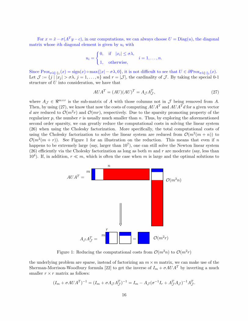
For x = x−σ(AT y− c), in our computations, we can always choose U = Diag(u), the diagonalmatrix whose ith diagonal element is given by ui with

ui =

0, if |xi| ≤ σλ,

1, otherwise,i = 1, . . . , n.

Since Proxσλ‖·‖1(x) = sign(x) max|x| − σλ, 0, it is not difficult to see that U ∈ ∂Proxσλ‖·‖1(x).Let J := j | |xj | > σλ, j = 1, . . . , n and r = |J |, the cardinality of J . By taking the special 0-1structure of U into consideration, we have that

AUAT = (AU)(AU)T = AJATJ , (27)

where AJ ∈ <m×r is the sub-matrix of A with those columns not in J being removed from A.Then, by using (27), we know that now the costs of computing AUAT and AUATd for a given vectord are reduced to O(m2r) and O(mr), respectively. Due to the sparsity promoting property of theregularizer p, the number r is usually much smaller than n. Thus, by exploring the aforementionedsecond order sparsity, we can greatly reduce the computational costs in solving the linear system(26) when using the Cholesky factorization. More specifically, the total computational costs ofusing the Cholesky factorization to solve the linear system are reduced from O(m2(m + n)) toO(m2(m + r)). See Figure 1 for an illustration on the reduction. This means that even if nhappens to be extremely large (say, larger than 107), one can still solve the Newton linear system(26) efficiently via the Cholesky factorization as long as both m and r are moderate (say, less than104). If, in addition, r m, which is often the case when m is large and the optimal solutions to

m

n

AUAT = O(m2n)

AJATJ =

m

r

= O(m2r)

Figure 1: Reducing the computational costs from O(m2n) to O(m2r)

the underlying problem are sparse, instead of factorizing an m×m matrix, we can make use of theSherman-Morrison-Woodbury formula [22] to get the inverse of Im + σAUAT by inverting a muchsmaller r × r matrix as follows:

(Im + σAUAT )−1 = (Im + σAJATJ )−1 = Im −AJ (σ−1Ir +ATJAJ )−1ATJ .

16

See Figure 2 for an illustration on the computation of ATJAJ . In this case, the total computationalcosts for solving the Newton linear system (26) are reduced significantly further from O(m2(m+r))to O(r2(m + r)). We should emphasize here that this dramatic reduction on the computationalcosts results from the wise combination of the careful examination of the existing second ordersparsity in the Lasso-type problems and some “smart” numerical linear algebra.

rm

=ATJAJ = O(r2m)

Figure 2: Further reducing the computational costs to O(r2m)

From the above arguments, we can see that as long as the number of the nonzero componentsof Proxσλ‖·‖1(x) is small, say less than

√n and Hj ∈ ∂(∇h∗)(yj) is a sparse matrix, e.g., a diagonal

matrix, we can always solve the linear system (24) at very low costs. In particular, this is truefor the Lasso problems admitting sparse solutions. Similar discussions on the reduction of thecomputational costs can also be conducted for the case when the conjugate gradient method isapplied to solve the linear systems (24). Note that one may argue that even if the original problemhas only sparse solutions, at certain stages, one may still encounter the situation that the numberof the nonzero components of Proxσλ‖·‖1(x) is large. Our answer to this question is simple. Firstly,this phenomenon rarely occurs in practice since we always start with a sparse feasible point, e.g.,the zero vector. Secondly, even at certain steps this phenomenon does occur, we just need toapply a small number of conjugate gradient iterations to the linear system (24) as in this case theparameter σ is normally small and the current point is far away from any sparse optimal solution.In summary, we have demonstrated how Algorithm Ssn can be implemented efficiently for solvingsparse optimization problems of the form (18) with p(·) being chosen to be λ‖ · ‖1.

4 Numerical experiments for Lasso problems

In this section, we shall evaluate the performance of our algorithm Ssnal for solving large scaleLasso problems (1). We note that the relative performance of most of the existing algorithmsmentioned in the introduction has recently been well documented in the two recent papers [18, 36],which appears to suggest that for some large scale sparse reconstruction problems, mfIPM1 andFPC AS2 have mostly outperformed the other solvers. Hence, in this section we will compare ouralgorithm with these two popular solvers. Note that mfIPM is a specialized interior-point basedsecond-order method designed for the Lasso problem (1), whereas FPC AS is a first-order methodbased on forward-backward operator splitting. Moreover, we also report the numerical performanceof two commonly used algorithms for solving Lasso problems: the accelerated proximal gradient(APG) algorithm as implemented by Liu et al. in SLEP3 [32] and the alternating direction methodof multipliers (ADMM) [19, 20]. For the purpose of comparisons, we also test the linearized ADMM(LADMM) [55]. We have implemented both ADMM and LADMM in Matlab with the step-length

1http://www.maths.ed.ac.uk/ERGO/mfipmcs/2http://www.caam.rice.edu/~optimization/L1/FPC_AS/3http://yelab.net/software/SLEP/

17

set to be 1.618. Although the existing solvers can perform impressively well on some easy-to-solvesparse reconstruction problems, as one will see later, they lack the ability to efficiently solve difficultproblems such as the large scale regression problems when the data A is badly conditioned.

For the testing purpose, the regularization parameter λ in the Lasso problem (1) is chosen as

λ = λc‖A∗b‖∞,

where 0 < λc < 1. In our numerical experiments, we measure the accuracy of an approximateoptimal solution x for (1) by using the following relative KKT residual:

η =‖x− proxλ‖·‖1(x−A∗(Ax− b))‖

1 + ‖x‖+ ‖Ax− b‖.

For a given tolerance ε > 0, we will stop the tested algorithms when η < ε. For all the tests in thissection, we set ε = 10−6. The algorithms will also be stopped when they reach the maximum numberof iterations (1000 iterations for our algorithm and mfIPM, and 20000 iterations for FPC AS,APG, ADMM and LADMM) or the maximum computation time of 7 hours. All the parametersfor mfIPM, FPC AS and APG are set to the default values. All our computational results areobtained by running Matlab (version 8.4) on a windows workstation (16-core, Intel Xeon E5-2650@ 2.60GHz, 64 G RAM).

4.1 Numerical results for large scale regression problems

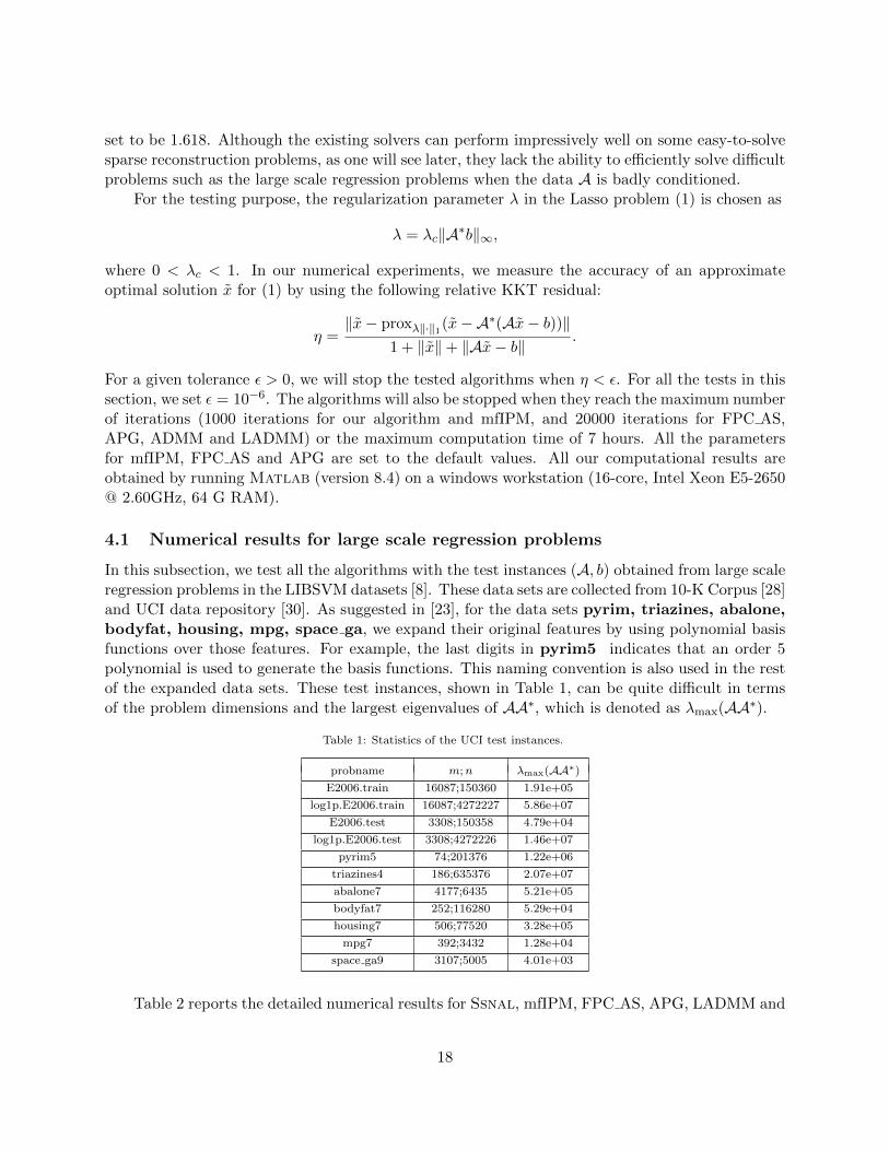
In this subsection, we test all the algorithms with the test instances (A, b) obtained from large scaleregression problems in the LIBSVM datasets [8]. These data sets are collected from 10-K Corpus [28]and UCI data repository [30]. As suggested in [23], for the data sets pyrim, triazines, abalone,bodyfat, housing, mpg, space ga, we expand their original features by using polynomial basisfunctions over those features. For example, the last digits in pyrim5 indicates that an order 5polynomial is used to generate the basis functions. This naming convention is also used in the restof the expanded data sets. These test instances, shown in Table 1, can be quite difficult in termsof the problem dimensions and the largest eigenvalues of AA∗, which is denoted as λmax(AA∗).

Table 1: Statistics of the UCI test instances.

probname m;n λmax(AA∗)E2006.train 16087;150360 1.91e+05

log1p.E2006.train 16087;4272227 5.86e+07

E2006.test 3308;150358 4.79e+04

log1p.E2006.test 3308;4272226 1.46e+07

pyrim5 74;201376 1.22e+06

triazines4 186;635376 2.07e+07

abalone7 4177;6435 5.21e+05

bodyfat7 252;116280 5.29e+04

housing7 506;77520 3.28e+05

mpg7 392;3432 1.28e+04

space ga9 3107;5005 4.01e+03

Table 2 reports the detailed numerical results for Ssnal, mfIPM, FPC AS, APG, LADMM and

18

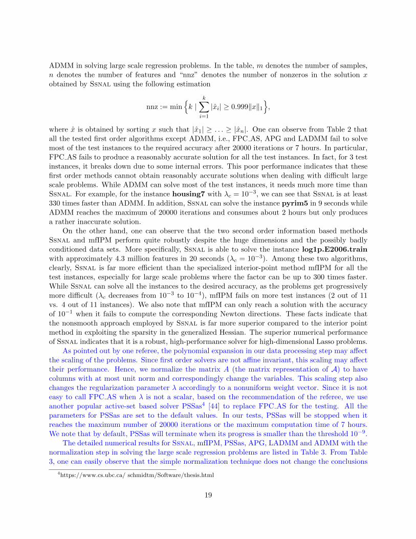
ADMM in solving large scale regression problems. In the table, m denotes the number of samples,n denotes the number of features and “nnz” denotes the number of nonzeros in the solution xobtained by Ssnal using the following estimation

nnz := mink |

k∑i=1

|xi| ≥ 0.999‖x‖1,

where x is obtained by sorting x such that |x1| ≥ . . . ≥ |xn|. One can observe from Table 2 thatall the tested first order algorithms except ADMM, i.e., FPC AS, APG and LADMM fail to solvemost of the test instances to the required accuracy after 20000 iterations or 7 hours. In particular,FPC AS fails to produce a reasonably accurate solution for all the test instances. In fact, for 3 testinstances, it breaks down due to some internal errors. This poor performance indicates that thesefirst order methods cannot obtain reasonably accurate solutions when dealing with difficult largescale problems. While ADMM can solve most of the test instances, it needs much more time thanSsnal. For example, for the instance housing7 with λc = 10−3, we can see that Ssnal is at least330 times faster than ADMM. In addition, Ssnal can solve the instance pyrim5 in 9 seconds whileADMM reaches the maximum of 20000 iterations and consumes about 2 hours but only producesa rather inaccurate solution.

On the other hand, one can observe that the two second order information based methodsSsnal and mfIPM perform quite robustly despite the huge dimensions and the possibly badlyconditioned data sets. More specifically, Ssnal is able to solve the instance log1p.E2006.trainwith approximately 4.3 million features in 20 seconds (λc = 10−3). Among these two algorithms,clearly, Ssnal is far more efficient than the specialized interior-point method mfIPM for all thetest instances, especially for large scale problems where the factor can be up to 300 times faster.While Ssnal can solve all the instances to the desired accuracy, as the problems get progressivelymore difficult (λc decreases from 10−3 to 10−4), mfIPM fails on more test instances (2 out of 11vs. 4 out of 11 instances). We also note that mfIPM can only reach a solution with the accuracyof 10−1 when it fails to compute the corresponding Newton directions. These facts indicate thatthe nonsmooth approach employed by Ssnal is far more superior compared to the interior pointmethod in exploiting the sparsity in the generalized Hessian. The superior numerical performanceof Ssnal indicates that it is a robust, high-performance solver for high-dimensional Lasso problems.

As pointed out by one referee, the polynomial expansion in our data processing step may affectthe scaling of the problems. Since first order solvers are not affine invariant, this scaling may affecttheir performance. Hence, we normalize the matrix A (the matrix representation of A) to havecolumns with at most unit norm and correspondingly change the variables. This scaling step alsochanges the regularization parameter λ accordingly to a nonuniform weight vector. Since it is noteasy to call FPC AS when λ is not a scalar, based on the recommendation of the referee, we useanother popular active-set based solver PSSas4 [44] to replace FPC AS for the testing. All theparameters for PSSas are set to the default values. In our tests, PSSas will be stopped when itreaches the maximum number of 20000 iterations or the maximum computation time of 7 hours.We note that by default, PSSas will terminate when its progress is smaller than the threshold 10−9.

The detailed numerical results for Ssnal, mfIPM, PSSas, APG, LADMM and ADMM with thenormalization step in solving the large scale regression problems are listed in Table 3. From Table3, one can easily observe that the simple normalization technique does not change the conclusions

4https://www.cs.ubc.ca/ schmidtm/Software/thesis.html

19

based on Table 2. The performance of Ssnal is generally invariant with respect to the scaling andSsnal is still much faster and more robust than other solvers. Meanwhile, after the normalization,mfIPM now can solve 3 more instances to the required accuracy. On the other hand, APG andthe ADMM type of solvers (i.e., LADMM and ADMM) perform worse than the un-scaled case.Besides, PSSas can only solve 5 out of 22 instances to the required accuracy. In fact, PSSas failson all the test instances when λc = 10−4. For the instance triazines4, it consumes about 6 hoursbut only generates a poor solution with η = 2.3× 10−2. (Actually, we also run PSSas on these testinstances without scaling and obtain similar performance. Detailed results are omitted to conservespace.) Therefore, we can safely conclude that the simple normalization technique employed heremay not be suitable for general first order methods.

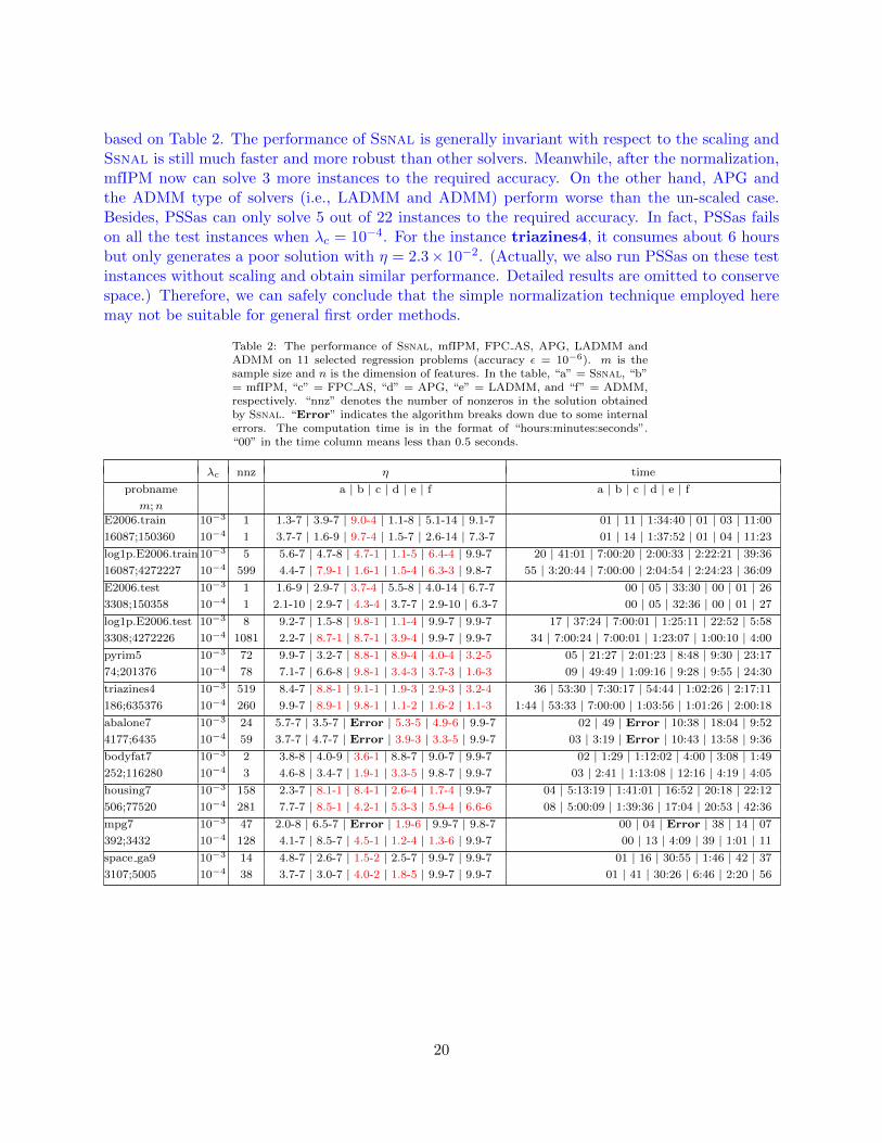
Table 2: The performance of Ssnal, mfIPM, FPC AS, APG, LADMM andADMM on 11 selected regression problems (accuracy ε = 10−6). m is thesample size and n is the dimension of features. In the table, “a” = Ssnal, “b”= mfIPM, “c” = FPC AS, “d” = APG, “e” = LADMM, and “f” = ADMM,respectively. “nnz” denotes the number of nonzeros in the solution obtainedby Ssnal. “Error” indicates the algorithm breaks down due to some internalerrors. The computation time is in the format of “hours:minutes:seconds”.“00” in the time column means less than 0.5 seconds.

λc nnz η time

probname a | b | c | d | e | f a | b | c | d | e | fm;n

E2006.train 10−3 1 1.3-7 | 3.9-7 | 9.0-4 | 1.1-8 | 5.1-14 | 9.1-7 01 | 11 | 1:34:40 | 01 | 03 | 11:0016087;150360 10−4 1 3.7-7 | 1.6-9 | 9.7-4 | 1.5-7 | 2.6-14 | 7.3-7 01 | 14 | 1:37:52 | 01 | 04 | 11:23log1p.E2006.train 10−3 5 5.6-7 | 4.7-8 | 4.7-1 | 1.1-5 | 6.4-4 | 9.9-7 20 | 41:01 | 7:00:20 | 2:00:33 | 2:22:21 | 39:3616087;4272227 10−4 599 4.4-7 | 7.9-1 | 1.6-1 | 1.5-4 | 6.3-3 | 9.8-7 55 | 3:20:44 | 7:00:00 | 2:04:54 | 2:24:23 | 36:09E2006.test 10−3 1 1.6-9 | 2.9-7 | 3.7-4 | 5.5-8 | 4.0-14 | 6.7-7 00 | 05 | 33:30 | 00 | 01 | 263308;150358 10−4 1 2.1-10 | 2.9-7 | 4.3-4 | 3.7-7 | 2.9-10 | 6.3-7 00 | 05 | 32:36 | 00 | 01 | 27log1p.E2006.test 10−3 8 9.2-7 | 1.5-8 | 9.8-1 | 1.1-4 | 9.9-7 | 9.9-7 17 | 37:24 | 7:00:01 | 1:25:11 | 22:52 | 5:583308;4272226 10−4 1081 2.2-7 | 8.7-1 | 8.7-1 | 3.9-4 | 9.9-7 | 9.9-7 34 | 7:00:24 | 7:00:01 | 1:23:07 | 1:00:10 | 4:00pyrim5 10−3 72 9.9-7 | 3.2-7 | 8.8-1 | 8.9-4 | 4.0-4 | 3.2-5 05 | 21:27 | 2:01:23 | 8:48 | 9:30 | 23:1774;201376 10−4 78 7.1-7 | 6.6-8 | 9.8-1 | 3.4-3 | 3.7-3 | 1.6-3 09 | 49:49 | 1:09:16 | 9:28 | 9:55 | 24:30triazines4 10−3 519 8.4-7 | 8.8-1 | 9.1-1 | 1.9-3 | 2.9-3 | 3.2-4 36 | 53:30 | 7:30:17 | 54:44 | 1:02:26 | 2:17:11186;635376 10−4 260 9.9-7 | 8.9-1 | 9.8-1 | 1.1-2 | 1.6-2 | 1.1-3 1:44 | 53:33 | 7:00:00 | 1:03:56 | 1:01:26 | 2:00:18abalone7 10−3 24 5.7-7 | 3.5-7 | Error | 5.3-5 | 4.9-6 | 9.9-7 02 | 49 | Error | 10:38 | 18:04 | 9:524177;6435 10−4 59 3.7-7 | 4.7-7 | Error | 3.9-3 | 3.3-5 | 9.9-7 03 | 3:19 | Error | 10:43 | 13:58 | 9:36bodyfat7 10−3 2 3.8-8 | 4.0-9 | 3.6-1 | 8.8-7 | 9.0-7 | 9.9-7 02 | 1:29 | 1:12:02 | 4:00 | 3:08 | 1:49252;116280 10−4 3 4.6-8 | 3.4-7 | 1.9-1 | 3.3-5 | 9.8-7 | 9.9-7 03 | 2:41 | 1:13:08 | 12:16 | 4:19 | 4:05housing7 10−3 158 2.3-7 | 8.1-1 | 8.4-1 | 2.6-4 | 1.7-4 | 9.9-7 04 | 5:13:19 | 1:41:01 | 16:52 | 20:18 | 22:12506;77520 10−4 281 7.7-7 | 8.5-1 | 4.2-1 | 5.3-3 | 5.9-4 | 6.6-6 08 | 5:00:09 | 1:39:36 | 17:04 | 20:53 | 42:36mpg7 10−3 47 2.0-8 | 6.5-7 | Error | 1.9-6 | 9.9-7 | 9.8-7 00 | 04 | Error | 38 | 14 | 07392;3432 10−4 128 4.1-7 | 8.5-7 | 4.5-1 | 1.2-4 | 1.3-6 | 9.9-7 00 | 13 | 4:09 | 39 | 1:01 | 11space ga9 10−3 14 4.8-7 | 2.6-7 | 1.5-2 | 2.5-7 | 9.9-7 | 9.9-7 01 | 16 | 30:55 | 1:46 | 42 | 373107;5005 10−4 38 3.7-7 | 3.0-7 | 4.0-2 | 1.8-5 | 9.9-7 | 9.9-7 01 | 41 | 30:26 | 6:46 | 2:20 | 56

20

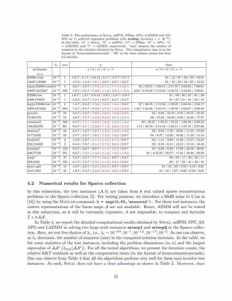
Table 3: The performance of Ssnal, mfIPM, PSSas, APG, LADMM and AD-MM on 11 selected regression problems with scaling (accuracy ε = 10−6).In the table, “a” = Ssnal, “b” = mfIPM, “c1” = PSSas, “d” = APG, “e”= LADMM, and “f” = ADMM, respectively. “nnz” denotes the number ofnonzeros in the solution obtained by Ssnal. The computation time is in theformat of “hours:minutes:seconds”. “00” in the time column means less than0.5 seconds.

λc nnz η time

probname a | b | c1 | d | e | f a | b | c1 | d | e | fm;n

E2006.train 10−3 1 1.6-7 | 4.1-7 | 4.6-12 | 9.1-7 | 8.7-7 | 9.7-7 01 | 14 | 01 | 02 | 05 | 10:2116087;150360 10−4 1 4.2-9 | 1.4-8 | 4.2-4 | 3.6-7 | 5.9-7 | 9.6-7 01 | 16 | 02 | 03 | 05 | 13:52log1p.E2006.train 10−3 5 2.6-7 | 4.9-7 | 1.7-6 | 1.7-4 | 1.7-4 | 2.8-5 35 | 59:55 | 1:29:14 | 2:17:57 | 3:05:04 | 7:00:0116087;4272227 10−4 599 5.0-7 | 3.6-7 | 8.8-6 | 1.1-2 | 3.2-3 | 1.0-4 2:04 | 2:18:28 | 5:19:39 | 2:34:51 | 3:10:05 | 7:00:01E2006.test 10−3 1 1.6-7 | 1.3-7 | 6.5-10 | 3.9-7 | 2.4-7 | 9.9-7 01 | 08 | 00 | 01 | 01 | 283308;150358 10−4 1 3.2-9 | 2.5-7 | 8.9-4 | 8.9-7 | 6.4-7 | 9.5-7 01 | 07 | 01 | 01 | 02 | 35log1p.E2006.test 10−3 8 1.4-7 | 9.2-8 | 1.5-6 | 1.6-2 | 1.9-4 | 9.9-7 27 | 30:45 | 1:13:58 | 1:29:25 | 2:08:16 | 2:30:173308;4272226 10−4 1081 7.2-7 | 8.5-7 | 9.4-6 | 3.7-3 | 1.3-3 | 2.9-4 1:40 | 1:24:36 | 5:45:18 | 1:30:58 | 2:02:07 | 3:06:48pyrim5 10−3 70 2.5-7 | 4.2-7 | 7.2-3 | 3.6-3 | 1.0-3 | 4.1-5 05 | 9:03 | 16:42 | 8:25 | 10:12 | 20:4874;201376 10−4 78 4.6-7 | 7.7-7 | 1.3-2 | 8.2-3 | 3.7-3 | 2.4-3 06 | 47:20 | 34:03 | 9:06 | 10:48 | 17:37triazines4 10−3 566 8.5-7 | 7.7-1 | 2.0-3 | 1.8-3 | 1.3-3 | 1.3-4 29 | 49:27 | 1:35:41 | 55:31 | 1:06:28 | 2:28:23186;635376 10−4 261 9.8-7 | 9.4-1 | 2.3-2 | 1.1-2 | 2.6-2 | 2.1-2 1:14 | 48:19 | 5:11:45 | 1:03:11 | 1:07:45 | 2:07:36abalone7 10−3 24 8.4-7 | 1.6-7 | 1.5-7 | 1.3-3 | 1.5-4 | 1.8-6 02 | 2:03 | 1:59 | 10:05 | 11:54 | 37:584177;6435 10−4 59 3.7-7 | 9.2-7 | 1.8-1 | 7.3-2 | 5.8-2 | 9.9-7 04 | 9:47 | 12:26 | 10:30 | 11:49 | 14:19bodyfat7 10−3 2 1.2-8 | 5.2-7 | 2.1-5 | 1.4-2 | 8.7-2 | 9.9-7 02 | 1:41 | 3:28 | 12:49 | 15:27 | 10:24252;116280 10−4 3 6.4-8 | 7.8-7 | 2.4-1 | 2.7-2 | 9.0-2 | 9.9-7 03 | 2:18 | 6:14 | 13:12 | 15:13 | 18:40housing7 10−3 158 8.8-7 | 6.6-7 | 9.9-7 | 4.1-4 | 5.5-6 | 9.9-7 03 | 6:26 | 9:20 | 17:00 | 25:56 | 20:06506;77520 10−4 281 8.0-7 | 7.0-1 | 1.4-5 | 1.1-2 | 1.9-3 | 1.3-5 05 | 4:33:23 | 30:27 | 17:34 | 19:46 | 49:20mpg7 10−3 47 5.2-7 | 3.5-7 | 7.7-7 | 2.6-4 | 9.9-7 | 9.9-7 00 | 05 | 11 | 40 | 46 | 11392;3432 10−4 128 6.1-7 | 7.5-7 | 3.3-5 | 1.1-3 | 2.3-4 | 9.9-7 00 | 17 | 56 | 41 | 50 | 10space ga9 10−3 14 4.3-7 | 2.3-7 | 2.2-5 | 9.3-5 | 9.9-7 | 9.9-7 01 | 34 | 03 | 5:59 | 4:18 | 3:213107;5005 10−4 38 1.6-7 | 5.4-7 | 2.4-5 | 2.3-3 | 3.6-3 | 9.9-7 01 | 49 | 1:07 | 6:00 | 6:48 | 3:02

4.2 Numerical results for Sparco collection

In this subsection, the test instances (A, b) are taken from 8 real valued sparse reconstructionproblems in the Sparco collection [5]. For testing purpose, we introduce a 60dB noise to b (as in[18]) by using the Matlab command: b = awgn(b,60,’measured’). For these test instances, thematrix representations of the linear maps A are not available. Hence, ADMM will not be testedin this subsection, as it will be extremely expensive, if not impossible, to compute and factorizeI + σAA∗.

In Table 4, we report the detailed computational results obtained by Ssnal, mfIPM, FPC AS,APG and LADMM in solving two large scale instances srcsep1 and srcsep2 in the Sparco collec-tion. Here, we test five choices of λc, i.e., λc = 10−0.8, 10−1, 10−1.2, 10−1.5, 10−2. As one can observe,as λc decreases, the number of nonzeros (nnz) in the computed solution increases. In the table, welist some statistics of the test instances, including the problem dimensions (m,n) and the largesteigenvalue of AA∗ (λmax(AA∗)). For all the tested algorithms, we present the iteration counts, therelative KKT residuals as well as the computation times (in the format of hours:minutes:seconds).One can observe from Table 4 that all the algorithms perform very well for these easy-to-solve testinstances. As such, Ssnal does not have a clear advantage as shown in Table 2. Moreover, since

21

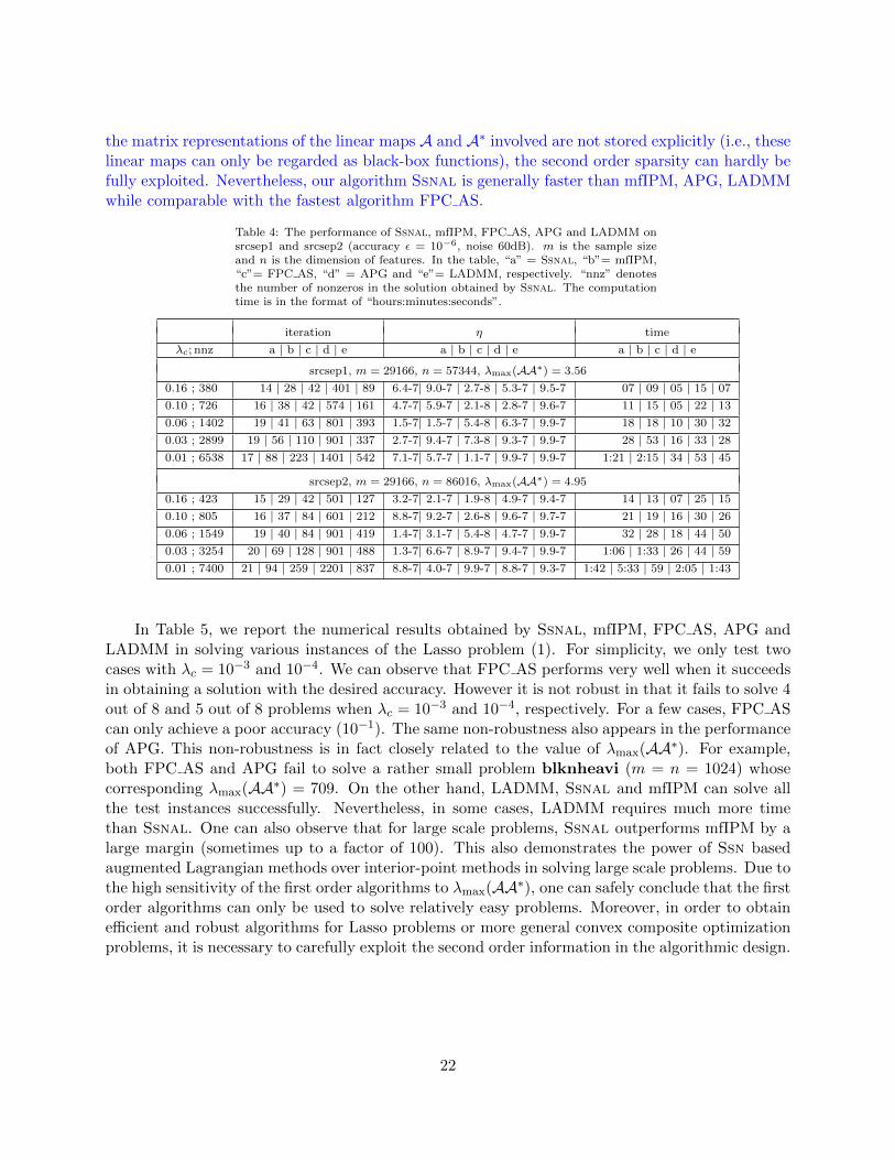
the matrix representations of the linear maps A and A∗ involved are not stored explicitly (i.e., theselinear maps can only be regarded as black-box functions), the second order sparsity can hardly befully exploited. Nevertheless, our algorithm Ssnal is generally faster than mfIPM, APG, LADMMwhile comparable with the fastest algorithm FPC AS.

Table 4: The performance of Ssnal, mfIPM, FPC AS, APG and LADMM onsrcsep1 and srcsep2 (accuracy ε = 10−6, noise 60dB). m is the sample sizeand n is the dimension of features. In the table, “a” = Ssnal, “b”= mfIPM,“c”= FPC AS, “d” = APG and “e”= LADMM, respectively. “nnz” denotesthe number of nonzeros in the solution obtained by Ssnal. The computationtime is in the format of “hours:minutes:seconds”.

iteration η time

λc; nnz a | b | c | d | e a | b | c | d | e a | b | c | d | e

srcsep1, m = 29166, n = 57344, λmax(AA∗) = 3.56

0.16 ; 380 14 | 28 | 42 | 401 | 89 6.4-7| 9.0-7 | 2.7-8 | 5.3-7 | 9.5-7 07 | 09 | 05 | 15 | 070.10 ; 726 16 | 38 | 42 | 574 | 161 4.7-7| 5.9-7 | 2.1-8 | 2.8-7 | 9.6-7 11 | 15 | 05 | 22 | 130.06 ; 1402 19 | 41 | 63 | 801 | 393 1.5-7| 1.5-7 | 5.4-8 | 6.3-7 | 9.9-7 18 | 18 | 10 | 30 | 320.03 ; 2899 19 | 56 | 110 | 901 | 337 2.7-7| 9.4-7 | 7.3-8 | 9.3-7 | 9.9-7 28 | 53 | 16 | 33 | 280.01 ; 6538 17 | 88 | 223 | 1401 | 542 7.1-7| 5.7-7 | 1.1-7 | 9.9-7 | 9.9-7 1:21 | 2:15 | 34 | 53 | 45

srcsep2, m = 29166, n = 86016, λmax(AA∗) = 4.95

0.16 ; 423 15 | 29 | 42 | 501 | 127 3.2-7| 2.1-7 | 1.9-8 | 4.9-7 | 9.4-7 14 | 13 | 07 | 25 | 150.10 ; 805 16 | 37 | 84 | 601 | 212 8.8-7| 9.2-7 | 2.6-8 | 9.6-7 | 9.7-7 21 | 19 | 16 | 30 | 260.06 ; 1549 19 | 40 | 84 | 901 | 419 1.4-7| 3.1-7 | 5.4-8 | 4.7-7 | 9.9-7 32 | 28 | 18 | 44 | 500.03 ; 3254 20 | 69 | 128 | 901 | 488 1.3-7| 6.6-7 | 8.9-7 | 9.4-7 | 9.9-7 1:06 | 1:33 | 26 | 44 | 590.01 ; 7400 21 | 94 | 259 | 2201 | 837 8.8-7| 4.0-7 | 9.9-7 | 8.8-7 | 9.3-7 1:42 | 5:33 | 59 | 2:05 | 1:43

In Table 5, we report the numerical results obtained by Ssnal, mfIPM, FPC AS, APG andLADMM in solving various instances of the Lasso problem (1). For simplicity, we only test twocases with λc = 10−3 and 10−4. We can observe that FPC AS performs very well when it succeedsin obtaining a solution with the desired accuracy. However it is not robust in that it fails to solve 4out of 8 and 5 out of 8 problems when λc = 10−3 and 10−4, respectively. For a few cases, FPC AScan only achieve a poor accuracy (10−1). The same non-robustness also appears in the performanceof APG. This non-robustness is in fact closely related to the value of λmax(AA∗). For example,both FPC AS and APG fail to solve a rather small problem blknheavi (m = n = 1024) whosecorresponding λmax(AA∗) = 709. On the other hand, LADMM, Ssnal and mfIPM can solve allthe test instances successfully. Nevertheless, in some cases, LADMM requires much more timethan Ssnal. One can also observe that for large scale problems, Ssnal outperforms mfIPM by alarge margin (sometimes up to a factor of 100). This also demonstrates the power of Ssn basedaugmented Lagrangian methods over interior-point methods in solving large scale problems. Due tothe high sensitivity of the first order algorithms to λmax(AA∗), one can safely conclude that the firstorder algorithms can only be used to solve relatively easy problems. Moreover, in order to obtainefficient and robust algorithms for Lasso problems or more general convex composite optimizationproblems, it is necessary to carefully exploit the second order information in the algorithmic design.

22

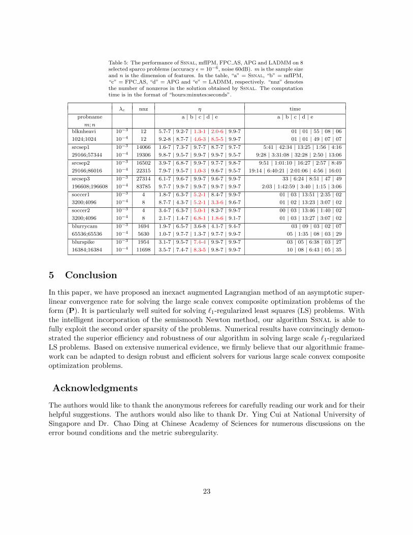
Table 5: The performance of Ssnal, mfIPM, FPC AS, APG and LADMM on 8selected sparco problems (accuracy ε = 10−6, noise 60dB). m is the sample sizeand n is the dimension of features. In the table, “a” = Ssnal, “b” = mfIPM,“c” = FPC AS, “d” = APG and “e” = LADMM, respectively. “nnz” denotesthe number of nonzeros in the solution obtained by Ssnal. The computationtime is in the format of “hours:minutes:seconds”.

λc nnz η time

probname a | b | c | d | e a | b | c | d | em;n

blknheavi 10−3 12 5.7-7 | 9.2-7 | 1.3-1 | 2.0-6 | 9.9-7 01 | 01 | 55 | 08 | 061024;1024 10−4 12 9.2-8 | 8.7-7 | 4.6-3 | 8.5-5 | 9.9-7 01 | 01 | 49 | 07 | 07srcsep1 10−3 14066 1.6-7 | 7.3-7 | 9.7-7 | 8.7-7 | 9.7-7 5:41 | 42:34 | 13:25 | 1:56 | 4:1629166;57344 10−4 19306 9.8-7 | 9.5-7 | 9.9-7 | 9.9-7 | 9.5-7 9:28 | 3:31:08 | 32:28 | 2:50 | 13:06srcsep2 10−3 16502 3.9-7 | 6.8-7 | 9.9-7 | 9.7-7 | 9.8-7 9:51 | 1:01:10 | 16:27 | 2:57 | 8:4929166;86016 10−4 22315 7.9-7 | 9.5-7 | 1.0-3 | 9.6-7 | 9.5-7 19:14 | 6:40:21 | 2:01:06 | 4:56 | 16:01srcsep3 10−3 27314 6.1-7 | 9.6-7 | 9.9-7 | 9.6-7 | 9.9-7 33 | 6:24 | 8:51 | 47 | 49196608;196608 10−4 83785 9.7-7 | 9.9-7 | 9.9-7 | 9.9-7 | 9.9-7 2:03 | 1:42:59 | 3:40 | 1:15 | 3:06soccer1 10−3 4 1.8-7 | 6.3-7 | 5.2-1 | 8.4-7 | 9.9-7 01 | 03 | 13:51 | 2:35 | 023200;4096 10−4 8 8.7-7 | 4.3-7 | 5.2-1 | 3.3-6 | 9.6-7 01 | 02 | 13:23 | 3:07 | 02soccer2 10−3 4 3.4-7 | 6.3-7 | 5.0-1 | 8.2-7 | 9.9-7 00 | 03 | 13:46 | 1:40 | 023200;4096 10−4 8 2.1-7 | 1.4-7 | 6.8-1 | 1.8-6 | 9.1-7 01 | 03 | 13:27 | 3:07 | 02blurrycam 10−3 1694 1.9-7 | 6.5-7 | 3.6-8 | 4.1-7 | 9.4-7 03 | 09 | 03 | 02 | 0765536;65536 10−4 5630 1.0-7 | 9.7-7 | 1.3-7 | 9.7-7 | 9.9-7 05 | 1:35 | 08 | 03 | 29blurspike 10−3 1954 3.1-7 | 9.5-7 | 7.4-4 | 9.9-7 | 9.9-7 03 | 05 | 6:38 | 03 | 2716384;16384 10−4 11698 3.5-7 | 7.4-7 | 8.3-5 | 9.8-7 | 9.9-7 10 | 08 | 6:43 | 05 | 35

5 Conclusion

In this paper, we have proposed an inexact augmented Lagrangian method of an asymptotic super-linear convergence rate for solving the large scale convex composite optimization problems of theform (P). It is particularly well suited for solving `1-regularized least squares (LS) problems. Withthe intelligent incorporation of the semismooth Newton method, our algorithm Ssnal is able tofully exploit the second order sparsity of the problems. Numerical results have convincingly demon-strated the superior efficiency and robustness of our algorithm in solving large scale `1-regularizedLS problems. Based on extensive numerical evidence, we firmly believe that our algorithmic frame-work can be adapted to design robust and efficient solvers for various large scale convex compositeoptimization problems.

Acknowledgments

The authors would like to thank the anonymous referees for carefully reading our work and for theirhelpful suggestions. The authors would also like to thank Dr. Ying Cui at National University ofSingapore and Dr. Chao Ding at Chinese Academy of Sciences for numerous discussions on theerror bound conditions and the metric subregularity.

23

References

[1] A. Y. Aravkin, J. V. Burke, D. Drusvyatskiy, M. P. Friedlander, and S. Roy, Level-setmethods for convex optimization, arXiv:1602.01506, 2016.

[2] A. Beck, and M. Teboulle, A fast iterative shrinkage-thresholding algorithm for linear inverseproblems, SIAM J. Imaging Sciences, 2 (2009), pp. 183–202.

[3] S. Becker, J. Bobin, and E. J. Candes, NESTA: A fast and accurate first-order method for sparserecovery, SIAM J. Imaging Sciences, 4 (2011), pp. 1–39.

[4] E. van den Berg and M. P. Friedlander, Probing the Pareto frontier for basis pursuit solutions,SIAM J. Scientific Computing, 31 (2008), pp. 890–912.

[5] E. van den Berg, M.P. Friedlander, G. Hennenfent, F.J. Herrman, R. Saab, and O.Yılmaz, Sparco: A testing framework for sparse reconstruction, ACM Trans. Math. Softw. 35 (2009),pp. 1–16.

[6] R. H. Byrd, G. M. Chin, J. Nocedal, and F. Oztoprak, A family of second-order methods forconvex `1-regularized optimization, Mathematical Programming, 159 (2016), pp. 435–467.

[7] R. H. Byrd, J. Nocedal, and F. Oztoprak, An inexact successive quadratic approximation methodfor L-1 regularized optimization, Mathematical Programming, 157 (2016), pp. 375–396.

[8] C.-C. Chang and C.-J. Lin, LIBSVM: A library for support vector machines, ACM Transactionson Intelligent Systems and Technology, 2 (2011), pp. 27:1–27:27.

[9] S. S. Chen, D. L. Donoho, and M. A. Saunders, Atomic decomposition by basis pursuit, SIAMJ. Scientific Computing, 20 (1998), pp. 33–61.

[10] F. Clarke, Optimization and Nonsmooth Analysis, John Wiley and Sons, New York, 1983.

[11] A. L. Dontchev and R. T. Rockafellar, Characterizations of Lipschitzian stability in nonlinearprogramming, Mathematical programming with data perturbations, Lecture notes in pure and appliedmathematics, Dekker, 195 (1998), pp. 65–82.

[12] Y. Cui, D. F. Sun, and, K.-C. Toh, On the asymptotic superlinear convergence of the augmentedLagrangian method for semidefinite programming with multiple solutions, arXiv:1610.00875, 2016.

[13] A. L. Dontchev and R. T. Rockafellar, Implicit Functions and Solution Mappings, SpringerMonographs in Mathematics, Springer 2009.

[14] F. Facchinei and J.-S. Pang, Finite-dimensional Variational Inequalities and ComplementarityProblems, Springer, New York, 2003.

[15] J. Fan, H. Fang, and L. Han, Challenges of big data analysis, National Science Review, 1 (2014),pp. 293–314.

[16] M. A. T. Figueiredo, R. D. Nowak, and S. J. Wright, Gradient projection for sparse recon-struction: Application to compressed sensing and other inverse problems, IEEE J. Selected Topics inSignal Processing, 1 (2007), pp. 586–597.

[17] A. Fischer, Local behavior of an iterative framework for generalized equations with nonisolated solu-tions, Mathematical Programming, 94 (2002), pp. 91–124.

[18] K. Fountoulakis, J. Gondzio, and P. Zhlobich, Matrix-free interior point method for compressedsensing problems, Mathematical Programming Computation, 6 (2014), pp. 1–31.

[19] D. Gabay and B. Mercier, A dual algorithm for the solution of nonlinear variational problems viafinite element approximations, Comput. Math. Appl. 2 (1976), pp. 17–40.

24

[20] R. Glowinski and A. Marroco, Sur lapproximation, par elements finis dordre un, et la resolu-tion, par penalisation-dualite, dune classe de problemes de Dirichlet non lineares, Revue FrancaisedAutomatique, Informatique et Recherche Operationelle, 9 (R-2) (1975), pp. 41–76.

[21] R. Goebel and R. T. Rockafellar, Local strong convexity and local Lipschitz continuity of thegradient of convex functions, J. Convex Analysis, 15 (2008), pp. 263–270.

[22] G. Golub and C. F. Van Loan, Matrix Computations, 3nd ed., Johns Hopkins University Press,Baltimore, MD, 1996.

[23] L. Huang, J. Jia, B. Yu, B. G. Chun, P. Maniatis, and M. Naik, Predicting execution time ofcomputer programs using sparse polynomial regression, In Advances in Neural Information ProcessingSystems, 2010, pp. 883–891.

[24] A. F. Izmailov, A. S. Kurennoy, and M. V. Solodov, A note on upper Lipschitz stability, errorbounds, and critical multipliers for Lipschitz-continuous KKT systems, Mathematical Programming,142 (2013), pp. 591–604.

[25] K. Jiang, D. F. Sun, and K.-C. Toh, A partial proximal point algorithm for nuclear norm regular-ized matrix least squares problems, Mathematical Programming Computation, 6 (2014), pp. 281-325.

[26] N. Keskar, J. Nocedal, F. Oztoprak, and A. Wachter, A second-order method for convex`1-regularized optimization with active-set prediction, Optimization Methods and Software, 31 (2016),pp. 605-621.

[27] D. Klatte, Upper Lipschitz behavior of solutions to perturbed C1,1 optimization problems, Mathemat-ical Programming, 88 (2000), pp. 169–180.

[28] S. Kogan, D. Levin, B. R. Routledge, J. S. Sagi, and N. A. Smith, Predicting risk fromfinancial reports with regression, NAACL-HLT 2009, Boulder, CO, May-June 2009.

[29] J. D. Lee, Y. Sun, and M. A. Saunders, Proximal Newton-type methods for minimizing compositefunctions, SIAM J. on Optimization, 24 (2014), pp. 1420–1443.

[30] M. Lichman, UCI Machine Learning Repository, http://archive.ics.uci.edu/ml/datasets.html.

[31] X. D. Li, D. F. Sun, and K.-C. Toh, QSDPNAL: A two-phase proximal augmented Lagrangianmethod for convex quadratic semidefinite programming, arXiv:1512.08872, 2015.

[32] J. Liu, S. Ji, and J. Ye, SLEP: Sparse Learning with Efficient Projections, Arizona State University,2009.

[33] Z.-Q. Luo and P. Tseng, On the linear convergence of descent methods for convex essentially smoothminimization, SIAM J. Control and Optimization, 30 (1992), pp. 408–425.

[34] F. J. Luque, Asymptotic convergence analysis of the proximal point algorithm, SIAM J. Control andOptimization, 22 (1984), pp. 277–293.

[35] R. Mifflin, Semismooth and semiconvex functions in constrained optimization, SIAM J. Control andOptimization, 15 (1977), pp. 959–972.

[36] A. Milzarek and M. Ulbrich, A semismooth Newton method with multidimensional filter global-ization for `1-optimization, SIAM J. Optimization, 24 (2014), pp. 298–333.

[37] Y. Nesterov, A method of solving a convex programming problem with convergence rate O(1/k2),Soviet Mathematics Doklady 27 (1983), pp. 372–376.

[38] L. Qi and J. Sun, A nonsmooth version of Newton’s method, Mathematical Programming, 58 (1993),pp. 353–367.

25

[39] S. M. Robinson, Some continuity properties of polyhedral multifunctions, in Mathematical Program-ming at Oberwolfach, vol. 14 of Mathematical Programming Studies, Springer Berlin Heidelberg, 1981,pp. 206–214.

[40] R. T. Rockafellar, Convex Analysis, Princeton University Press, Princeton, N.J., 1970.

[41] R. T. Rockafellar, Monotone operators and the proximal point algorithm, SIAM J. Control andOptimization, 14 (1976), pp. 877–898.

[42] R. T. Rockafellar, Augmented Lagrangians and applications of the proximal point algorithm inconvex programming, Mathematics of Operations Research, 1 (1976), pp. 97–116.

[43] R. T. Rockafellar and R. J.-B. Wets, Variational Analysis, vol. 317 of Grundlehren der Mathe-matischen Wissenschaften [Fundamental Principles of Mathematical Sciences], Springer-Verlag, Berlin,1998.

[44] M. Schmidt, Graphical Model Structure Learning with `1-Regularization, PhD thesis, Department ofComputer Science, The University of British Columbia, 2010.

[45] D. F. Sun and J. Sun, Semismooth matrix-valued functions, Mathematics of Operations Research,27 (2002), pp. 150–169.

[46] J. Sun, On monotropic piecewise quadratic programming, PhD thesis, Department of Mathematics,University of Washington, 1986.

[47] P. Tseng and S. Yun, A coordinate gradient descent method for nonsmooth separable minimization,Mathematical Programming, 125 (2010), pp. 387–423.

[48] R. Tibshirani, Regression shrinkage and selection via the lasso, J. Royal Statistical Society: SeriesB, 58 (1996), pp. 267–288.

[49] Z. Wen, W. Yin, D. Goldfarb, and Y. Zhang, A fast algorithm for sparse reconstruction basedon shrinkage, subspace optimization, and continuation, SIAM J. Scientific Computing, 32 (2010),pp. 1832–1857.

[50] S. J. Wright, R. D. Nowak, and M. A. T. Figueiredo, Sparse reconstruction by separableapproximation, IEEE Trans. Signal Process., 57 (2009), pp. 2479–2493.

[51] X. Xiao, Y. Li, Z. Wen, and L. Zhang, Semi-smooth second-order type methods for compositeconvex programs, arXiv:1603.07870, 2016.

[52] L. Yang, D. F. Sun, and K.-C. Toh, SDPNAL+: A majorized semismooth Newton-CG aug-mented Lagrangian method for semidefinite programming with nonnegative constraints, MathematicalProgramming Computation, 7 (2015), pp. 331–366.

[53] M.-C. Yue, Z. Zhou, and A. M.-C. So, Inexact regularized proximal Newton method: provable con-vergence guarantees for non-smooth convex minimization without strong convexity, arXiv:1605.07522,2016.

[54] X. Zhao, D. F. Sun, and K.-C. Toh, A Newton-CG augmented Lagrangian method for semidefiniteprogramming, SIAM J. Optimization, 20 (2010), pp. 1737–1765.

[55] X. Zhang, M. Burger and S. Osher, A unified primal-dual algorithm framework based on Bregmaniteration, J. Scientific Computing, 49 (2011), pp. 20–46.

[56] H. Zhou, The adaptive Lasso and its oracle properties, J. American Statistical Association, 101 (2006),pp. 1418–1429.

[57] H. Zhou and T. Hastie, Regularization and variable selection via the elastic net, J. Royal StatisticalSociety, Series B, 67 (2005), pp. 301–320.

[58] Z. Zhou and A. M.-C. So, A unified approach to error bounds for structured convex optimizationproblems, Mathematical Programming, (2017), DOI:10.1007/s10107-016-1100-9.

26