A Leverage Theory of Tying in Two-Sided Markets�

Jay Pil Choiy Doh-Shin Jeonz

March 12, 2017

Abstract

Motivated by recent antitrust cases in markets with zero-pricing, we develop a lever-

age theory of tying in two-sided markets. In the presence of the non-negative price

constraint, tying provides a mechanism to circumvent the constraint in the tied mar-

ket without inviting aggressive responses by the rival �rm. We identify conditions

under which tying in two-sided markets is pro�table and explore its welfare impli-

cations. In addition, we show that our model can be applied more widely to any

markets in which sales to consumers in one market can generate additional revenues

that cannot be competed away due to non-negative price constraints.

JEL Codes: D4, L1, L5

KeyWords: Tying, Leverage of monopoly power, Two-sided markets, Zero pricing,

Non-negative pricing constraint

�We thank Andrea Amelio, Bernard Caillaud, Guillermo Caruana, Federico Etro, Giulio Federico,Bruno Jullien, Gerard Llobet, Andras Niedermayer, Volker Nocke, Martin Peitz, Patrick Rey, KyoungwonRhee, Chengsi Wang and participants in various conferences and seminars for valuable discussions andcomments. Taeyoon Hwang and Sungwook Koh provided excellent research assistance. This work wassupported by the Ministry of Education of the Republic of Korea and the National Research Foundationof Korea (NRF-2016S1A5A2A01022389). Jeon acknowledges the �nancial support of the Jean-JacquesLa¤ont Digital Chair.

yDepartment of Economics, Michigan State University and Hitotsubashi Institute for Advanced Study,Hitotsubashi University. E-mail: choijay@msu.edu.

zToulouse School of Economics, University of Toulouse Capitole (IDEI) and CEPR. E-mail:dohshin.jeon@gmail.com.

1 Introduction

We develop a leverage theory of tying in two-sided markets. We analyze incentives for a

monopolist to tie its monopolized product with products facing competition in two-sided

markets. We uncover a new channel through which a monopolistic �rm in one market

can leverage its monopoly power to another competing market if the latter is two-sided

and derive its welfare implications.

Our analysis, motivated by recent antitrust cases in markets with zero-pricing, applies

when platforms in a two-sided market are constrained to set non-negative prices on the

consumer side.1 In two-sided markets the need for all sides of the market to engage

creates a �chicken and egg�problem (Caillaud and Jullien, 2003) in that members of each

group are willing to participate in the market only if they expect many members from the

other side to participate. The literature on two-sided markets has analyzed the optimal

pricing structure to coordinate the demands of distinct groups of customers and shows

that below-cost pricing naturally arises on one side in order to enhance participation

because the loss from the below-cost pricing can be recouped on the other side of the

market (see Armstrong (2006) and Rochet and Tirole (2006)). When the marginal cost is

low as in digital markets, this implies that the optimal pricing strategy entails negative

prices. However, we can imagine situations in which negative prices may be impractical

due to adverse selection and opportunistic behaviors by consumers (Farrell and Gallini

(1988) and Amelio and Jullien (2012)).2

We show that tying provides a mechanism to circumvent the non-negative price con-

straint in the tied product market without inviting an aggressive response by the rival

�rm if the rival �rm�s price response to tying faces the non-negative constraint. In our

model, the non-negative price constraint plays two roles: 1) it limits competition in the

tied good market, which creates additional surplus to extract through tying, and 2) it lim-

its the rival �rm�s response to tying. In addition, our theory �lls the gap in the literature

by showing that tying is credible without any commitment mechanism and forecloses the

rival in the tied product market regardless of whether the two products tied together are

independent or complementary. The credibility of tying can explain the use of contractual

tying (such as Google�s contract with handset manufacturers) for the leverage purpose.3

1For a discussion of how to apply antiturst law to zero-price markets, including the issues of marketde�nition and market power, from the legal perspective, see Newman (2015, 2016).

2To quote Farrell and Gallini (1988), "[a]t a negative price, people could take computers at a negativeprice and use them for land�ll (p.679)."

3The tying literature distinguishes contractual tying from technical tying: the former can be undone

1

To see the incentives to leverage monopoly power, consider a monopolist in one market

that also competes in a two-sided market with a more e¢ cient rival �rm (i.e., a rival

platform). The two-sided market consists of consumers on one side and advertisers on

the other. We envision a situation in which consumers are competitive bottleneck in the

two-sided market (see Armstrong (2006) and Armstrong and Wright (2007)); a platform

can extract extra revenues from the advertiser side when it attracts a consumer from the

bottleneck side. First, in the absence of tying, the non-negative price constraint limits

competition on the consumer side of the two-sided market and generates additional pro�t

for the more e¢ cient rival �rm which cannot be competed away. This creates incentives for

the monopolistic �rm to tie and e¤ectively engage in a negative price in order to capture

this extra surplus. Second, when the monopolistic �rm tries to steal the additional pro�t

in the two-sided market, tying will induce a more aggressive response by the rival �rm

as in Whinston (1990). However, the rival �rm�s ability to respond aggressively can be

muted as the non-negative price constraint begins to bind. Thus, the non-negative price

constraint in two-sided markets plays the dual role of creating additional surplus and

limiting aggressive response by the rival �rm, which provides incentives to tie by the

monopolistic �rm.

The paper is partly motivated by the recent antitrust investigations concerning Google

in Europe and elsewhere.4 In one of the investigations, the European Commission (EC)

is concerned with Google�s conduct in relation to applications and services for smart-

phones and tablets.5 In particular, Google has been alleged by rival �rms to "illegally

hinder the development and market access of rival applications and services by tying or

bundling certain Google applications and services distributed on Android devices with

other Google applications, services and/or application programing interfaces of Google."6

ex post with a relatively low cost while the latter can be undone only with a signi�cant cost. There-fore, technical tying can be used as a device to pre-commit to tying when tying is not ex post credible(Whinston, 1990).

4Russian antitrust o¢ cials �ned Google $6.8 million on August 11, 2016 for abusing its market positionwith its mobile operating system Android. Google is also under investigation in Korea and India. To theextent that the web browser and the media player markets are two-sided, our model can also be appliedto the Microsoft tying cases in Europe and elsewhere.

5The EC�s other investigations on Google concern Google�s search engine, which has been alleged tobias its search results to promote other revenue-generating Google services such as comparison shop-ping. See the European Commission Fact Sheet entitled "Antitrust: Commission sends Statementof Objections to Google on comparison shopping service," released on April 15, 2015. Available athttp://europa.eu/rapid/press-release_MEMO-15-4781_en.htm

6See the European Commission Fact Sheet entitled "Antitrust: Commission opens formal investigationagainst Google in relation to Android mobile operating system," released on April 15, 2015. Available

2

After preliminary investigations, the EC issued a statement of objections on April 20,

2016, informing Google of its view that "the company has, in breach of EU antitrust

rules, abused its dominant position by imposing restrictions on Android device manufac-

turers and mobile network operators."7 Even though Google�s Android operating system

for mobile devices is supposed to be "open," Google e¤ectively implements bundling of its

apps through Android�s Mobile Application Distribution Agreements (MADA) contracts

that force manufacturers to include them and their respective terms in an all-or-nothing

fashion.8 According to MADA contracts, Android device manufacturers must preinstall

all or none of Google apps, depriving them of the ability to mix and match Google apps

considered essential with other third-party apps which may be superior to some of the

listed Google apps. Even though they are allowed to preinstall competing apps in ad-

dition to the listed Google apps with similar functionalities, they are reluctant to do so

because of the limited screen space available on devices and potential user confusion.9 In

addition, Google requires its apps to be the default in key app categories such as search

and location and be placed in prominent positions on the screen.10 As a result, the po-

tential for installing multiple apps (i.e., multihoming) to mitigate the e¤ects of tying is

somewhat limited (Edelman, 2015). The EC�s analysis in relation to the investigation of

Google also indicates that "consumers rarely download applications that would provide

the same functionality as an app that is already pre-installed (unless the pre-installed app

is of particularly poor quality)."11 The tying mechanism we uncover can be applied to

the Google Android case and can explain why Google has an incentive to tie. We further

show that such tying arrangements can lead to the exclusion of (more e¢ cient) rival �rms,

providing a theory of harm associated with Google�s practices in the MADA contracts.12

at http://europa.eu/rapid/press-release_MEMO-15-4782_en.htm7See the European Commission Press Release entitled "Antitrust: Commission sends State-

ment of Objections to Google on Android operating system and applications," available athttp://europa.eu/rapid/press-release_IP-16-1492_en.htm

8"Devices may only be distributed if all Google Applications [listed elsewhere in the agreement] ... arepre-installed on the Device." See section 2.1 of the MADA between Google and HTC.

9Other considerations that limit pre-installation of competing apps include their impacts on RAM,battery life, and limited storage space.10For instance, the phone manufacturer must set �Google Search ... as the default search provider for

all Web search access points.� See MADA Section 3.4(4). The same requirement applies to Google�sNetwork Location Provider service.11See the European Commission - Fact Sheet entitled "Antitrust: Commission sends Statement of

Objections to Google on Android operating system and applications,�released on April 20, 2016. Availableat http://europa.eu/rapid/press-release_MEMO-16-1484_en.htm.12For a detailed discussion of the key aspects of Google�s practices and their potentially exclusionary

e¤ects in the mobile phone industry from a legal perspective, see Edelman and Geradin (2016).

3

In Section 2, we present our mechanism of tying in the baseline model of homogenous

consumers. In a setting in which the well-known "single monopoly pro�t result" holds if

the tied market is one-sided (or in the absence of the non-negative price constraint), we

show that the interplay between two-sidedness of the tied market and the non-negative

pricing constraint breaks the result and restores an incentive to tie to leverage monopoly

power into the tied two-sided market. In addition, this mechanism is robust even when

consumers can multi-home (section 2.2) and when the bundled products are perfect com-

plements instead of having independent values (section 2.3).

In section 3, we show that our insight is not limited to two-sided markets and can

be more widely applied to any markets in which sales to consumers in one market can

generate additional revenues that cannot be competed away due to non-negative price

constraints. Speci�cally, even if the tied market is one-sided, additional revenue can be

generated in an intertemporal context from the same market in the future in the presence

of network e¤ects (section 3.1) or switching costs (section 3.2). Section 4 brie�y discusses

two extensions of the baseline model which incorporate heterogenous consumers in the

tying market: the two extensions di¤er in terms of whether or not they consider cross-side

network e¤ects. These extensions allow us to check the robustness of our insight obtained

from the baseline model and also address the question of how the degree of two-sidedness

of the tying market a¤ects the incentive to tie.13 The details are relegated to the Web

Appendix (for online publication).

Our paper contributes to the literature on the leverage theory of tying, which has been

extensively studied. In a classical paper on tying, Whinston (1990) shows that selling a

monopolized primary product and an unrelated di¤erentiated product together as a bundle

may allow the monopolist to commit to a more aggressive pricing strategy, preventing

entry in the di¤erentiated market. In Carbajo, De Meza, and Seidman (1990), on the other

hand, bundling is used as a strategy to segment the market and relax price competition.14

By considering a model in which each of the tying and the tied markets can be one-

sided or two-sided (with the details in the Web Appendix), our paper encompasses both

Whinston�s and Carbajo et al.�s results as special cases. In particular, when the tied market

is two-sided, we uncover a new channel through which tying is pro�table at the expense

of rival �rms. We emphasize that our leverage mechanism does not have any credibility

13In the baseline model of homogenous consumers, the incentive to tie does not depend on the degreeof two-sidedness of the tying market.14See also Chen (1997).

4

issue in sharp contrast to Whinston (1990) and Nalebu¤ (2004). Our mechanism thus

does require neither technical tying as a commitment device as in Whinston (1990) nor

the assumption that the tying �rm is a Stackelberg leader in setting prices as in Nalebu¤

(2004).15 We show that a monopolist�s tying is credible and reduces the rival�s pro�t if the

tied market is two-sided, which provides a justi�cation for the use of contractual tying.

We further show that tying is credible and forecloses the rival even in the case of perfect

complements. This result is noteworthy because it is known that a monopolist selling a

perfectly complementary product has no incentive to practice tying to exclude the rival

(Proposition 3 of Whinston, 1990).

Choi and Stefanadis (2001) and Carlton and Waldman (2002) provide a dynamic lever-

age theory of tying. In Choi and Stefanadis (2001), the probability of successful entry

depends on the level of R&D expenditures. When an incumbent monopolist in two com-

plementary components practices bundling, it makes entry in one component completely

dependent upon success in the other. By making the prospects of investment less cer-

tain, bundling discourages rivals from investing and innovating. Carlton and Waldman

(2002) construct a related model of bundling with dynamic entry deterrence. In their two-

period model, the incumbent initially has a monopoly position in both the primary and

the complementary market. They show that the incumbent can maintain its monopoly

pro�ts in both periods when successful entry requires a two-step process of entering the

complementary market in period 1 and the primary market in period 2. However, these

two papers as well as most papers in the literature consider one-sided markets. We show

how the two-sidedness of markets in conjunction with the non-negative price constraint

generates a new channel through which monopoly power in one market can be leveraged

into another.

Amelio and Jullien (2012) analyze the e¤ects of tying in two-sided markets. They

consider a situation in which platforms would like to set prices below zero on one side

of the market to solve the demand coordination problem in two-sided markets, but are

constrained to set non-negative prices. In the analysis of Amelio and Jullien, tying can

15A notable exception is Peitz (2008), who points out the credibility issue and builds an examplein which a monopolist�s tying is credible and reduces the rival�s pro�t. Hurkens, Jeon and Menicucci(2016) restores credibility by considering that the tying �rm is not a monopolist but a dominant �rmfacing competition in the tying market. In the context of competition among product portfolios in acommon agency setting, Jeon and Menicucci (2006, 2012) �nd that pure bundling is credible as it reducescompetition among the products within a �rm�s portfolio but that competitive bundling leads to e¢ cientoutcome if the buyer has no budget constraint (otherwise, bundling builds an entry barrier since it allows�rms with large portfolios to capture all the budget).

5

serve as a mechanism to introduce implicit subsidies on one side of the market in order

to solve the aforementioned coordination failure in two-sided markets. As a result, tying

can raise participation on both sides and can bene�t consumers in the case of a monopoly

platform. In a duopoly context, however, tying also has a strategic e¤ect on competition.

They show that the e¤ects of tying on consumer surplus and social welfare depend on

the extent of asymmetry in externalities between the two sides. Their paper and ours are

very di¤erent in terms of focus and mechanisms through which tying a¤ects competition.

Their main focus is to compare the e¤ects of tying across di¤erent market structures

(monopolistic vs. duopolistic) whereas our focus is on the leverage of monopoly power in

two-sided markets. Choi (2010) also analyzes tying in two-sided markets. However, his

focus is on the role of multi-homing. In particular, he shows that tying can be welfare-

enhancing if multi-homing is allowed, even in cases where its welfare impacts are negative

in the absence of multi-homing.

Finally, Iacobucci (2014) develops a similar idea to our mechanism. In particular, he

argues that the elimination of competition in one side of the market, via tying of two

platforms, can expand the set of customers to whom the tying �rm can sell in the other

side of the market. This is similar to our mechanism in which capturing the customer

side provides additional revenue from the advertiser side. However, he does not provide

a formal analysis as his argument is based on a numerical example. In addition, his logic

breaks down when the non-negative price constraint is not binding as the same e¤ects

can be achieved by an appropriate pricing scheme without the use of tying. This is due

to his implicit assumption that �rms set prices equal to marginal costs in a competitive

equilibrium. In the context of complementary products envisioned in his model, however,

the equilibrium price in each component market need not be equal to marginal cost

because it is the total price, not the two individual prices, that matters for complementary

products. In contrast, we provide a rigorous and formal analysis of tying that fully accounts

for intricacies of two-sided markets.

The rest of the paper is organized in the following way. In Section 2, we present the

baseline model of homogenous consumers to highlight the main essence of the leverage

mechanism in two-sided markets and the importance of the non-negative price constraint.

We also establish the robustness of our mechanism to multihoming and perfect comple-

ments. In Section 3, we demonstrate the applicability of our insight to other types of

markets with auxiliary revenues. In the Web Appendix (for online publiction), we extend

the baseline model by introducing heterogenous consumers in the tying market and in-

6

vestigate how the two-sidedness of both the tying and tied product markets interact to

draw policy implications. We also consider a model with inter-group network e¤ects in

the tied good market. Section 4 contains a summary of the results presented in the Web

Appendix. We provide concluding remarks in Section 5. Detailed proofs are relegated to

the Appendix.

2 The Baseline Model of Homogenous Consumers

To show how the interaction between the two-sidedness of markets and the non-negative

price constraint generates new incentives to tie, we start by analyzing a simple baseline

model of homogenous consumers. In order to highlight the leverage mechanism in two-

sided markets, we consider a setting in which the well-known "single monopoly pro�t"

result holds and hence the extension of monopoly power from one market to another is

not possible in the benchmark without two-sided markets.

Consider two markets, A and B. We build a simple framework to analyze tying as a

leverage mechanism when both markets are characterized as two-sided. More speci�cally,

in each market there are three classes of agents. There are two distinct customer groups

(consumers and advertisers) that interact with each other and intermediaries which enable

these two groups to �meet�with each other. In the example of the Internet search market,

the two customer groups can be described as advertisers and consumers (who search for

information through the Internet). The intermediaries are search engine providers such

as Google and Bing. We assume that the two markets are independent in the sense that

the value that each consumer (or advertiser) derives from participating in a market is

independent of whether he or she participates in the other market.

To analyze incentives to leverage market power, we assume that market A is served

by �rm 1, a monopolistic platform, and entry to market A is not possible. In contrast,

two platforms, �rm 1 and �rm 2, compete in market B. More speci�cally, we envision

a competitive bottleneck situation in which platforms provide services (such as Internet

search and video streaming) to consumers and use the customer base to derive advertising

revenues from advertisers who need access to consumers. There is a mass one of identical

consumers, who have a unit demand for each service/product. To focus on the strategic

motive for bundling, we assume that there is no cost advantage or disadvantage associated

with bundling.

In market A, each consumer�s reservation value is denoted by u. In market B, each

7

consumer�s willingness to pay for each �rm�s product is given by v1 and v2, respectively,

where � � v2 � v1 > 0.16 For most of the paper, we assume that each consumer buys

only one of the two products in market B and normalize �rms�production costs to zero

in all markets.17 This single-homing assumption is relaxed in Section 2.2. Each consumer

yields additional pro�t of � � 0 and � � 0 to the advertiser side in market A and B,

respectively.18 If � = 0, the tying market is one-sided and if � = 0, the tied market is

one-sided.

2.1 The Leverage Mechanism with the Non-Negative Price Constraint inTwo-Sided Markets

Consider the benchmark in which both markets are one-sided (i.e., � = � = 0). If

these products are sold independently without tying, �rm 1 will charge pA1 = u in its

monopolized market A. In market B, both �rms compete in prices and the equilibrium

prices are given by pB1 = 0 and pB2 = �, where � � v2 � v1 > 0. All consumers buy from

�rm 2. Each �rm�s pro�ts are given by

�1 = �A1 + �B1 = u+ 0 = u;

�B2 = �:

Now suppose that �rm 1 ties its monopolized product A with product B1: Let eP andep2 denote the bundle price and �rm 2�s price for product B under tying.19 We assume

that a consumer buys either the (A;B1) bundle or product B2: this assumption is relaxed

by allowing multi-homing in section 2.2. Then, �rm 1 will be able to sell its bundled

products only if

u+ v1 � eP � v2 � ep2:Since �rm 2 will be willing to set the price as low as its marginal cost, which is zero,

16This is a standard assumption in the leverage theory of tying to analyze potential exclusion of moree¢ cient rival �rms. This assumption is made to facilitate comparison with the prior literature, andshould not be taken to imply that Google products are inferior to rival �rms�.17This is not an innocuous normalization assumption with the non-negative price constraint because

it also implies no below-cost pricing. However, as long as production costs are not too high (as wouldbe the case for digital goods), our results would be robust even if we allow below-cost pricing. Moreimportantly, we can derive qualitatively similar results when we introduce asymmetry between the two�rms in market B in terms of production costs rather than product qualities.18Alternatively, � and � can represent additional revenues coming from sale of consumer data to third

parties or in-app purchases. See de Cornière and Taylor (2016).19We denote variables under the tying regime with a tilde (~).

8

the maximum price �rm 1 can charge for its bundle in order to make sales is given byeP = u��: Under tying, �rm 1�s pro�t is given by

e�1 = max[u��; 0];which is less than the pro�t without tying as e�1 = max[u��; 0] < u = �1.20 Thus, evenif tying provides a mechanism to capture the tied good market, it is a Pyrrhic victory as

it reduces �rm 1�s pro�ts. Thus, the monopoly �rm has no incentives to tie to extend its

market power to the other market. This is the essence of the Chicago school�s criticism of

the leverage theory of tying. However, this conclusion can be overturned if the tied good

market B is two-sided.

Suppose now that market B is two-sided while market A is one-sided. Assume that

the advertising revenue is large enough in market B such that � > � holds.21 Due to

this additional revenue source, now each �rm in market B is willing to set its price below

its marginal cost on the consumer side up to �. We, however, put a non-negative price

restriction that the market prices cannot be negative. Thus, in the absence of tying, once

again �rm 1 charges a price of pB1 = 0 and �rm 2 will set the price of pB2 = �. Firm 1�s

pro�t in market B is zero. However, note that �rm 2�pro�t is given by �B2 = �+ � due

to the additional revenue from the advertiser side.

Now suppose that �rm 1 ties its monopolized product with product B on the consumer

side. Assume u > � such that �rm 1 can conquer market B by tying. Once again, the

maximum bundle price that enables the tying �rm to make sales is given by eP = u��:However, due to the additional revenue source in market B, the tying �rm�s pro�t now

becomes e�1 = u + (� ��) > u = �1: Hence, tying is pro�table if the tied good marketis two-sided.

Tying reduces welfare because it induces consumers to use the inferior product of

�rm 1. However, consumers bene�t from tying due to reduced prices. Consumer surplus

without tying can be expressed as CS = (u+ v2)� (u+�) = v1: With tying, consumersurplus is fCS = (u + v1) � (u ��) = v1 + � = v2(> v1 = CS). This may explain why

the driving force behind the European action was a consortium of Google�s competitors

rather than consumers (Stewart, 2016).22

20If v1 � v2, �rm 1�s pro�t with tying is the same as the one without tying.21According to the estimates by �nancial analyst Richard Windsor, Google made about $11 billion in

2015 from advertising sales on Android phones through its apps such as Maps, Search and Gmail. SeeChee (2016).22However, we should emphasize that this result on consumer surplus is not robust to heterogenous

9

This simple model also illustrates the importance of the non-negative price constraint

for the two-sidedness of the market to restore incentives to tie.23 To see this, suppose that

�rms can charge a negative price. Then, after tying �rm 2 would be willing to set the

price as low as ��: Thus, the maximum bundle price that enables the tying �rm to makesales is now given by eP = u �� � �: As a result, the tying �rm�s pro�t is now reducedto e�1 = u�� < u = �1 as in the Chicago school benchmark case above.As the non-negative price constraint is essential to our leverage mechanism, the ap-

plicability of our theory depends on the plausibility of the constraint. Whether the con-

straint is binding or not may depend on market characteristics. In the credit card industry,

for instance, cashback reward programs that o¤er rebates on card holders�purchases can

be considered as a negative price. In this case, however, there is a built-in mechanism

to prevent moral hazard and abuse of the program because consumers are not expected

to spend 100 dollars just to receive a 1 dollar rebate. Thus, the non-negative price con-

straint in the credit card industry is less plausible. By contrast, in the case of search

engines the constraint is more binding. To see this, suppose that Google pays a small

amount of money to anyone performing a Google search. There would be consumers

who do Google searches all day just to collect money, or people could create a software

program that does automated search on their behalf. Such behaviors would undermine

Google�s business model, because the only reason advertisers pay money to Google is for

targeted advertising tailored to those who do real searches. The same logic applies if we

interpret � as revenues from in-app purchases. The app producers can generate � only

from consumers who actually use the program. With freebies or a negative price, there

can be consumers who receive free items or free money from the app but never actually

use it and thus do not make any in-app purchases.

Finally, we can consider the case in which the tying market is two-sided (i.e., � > 0).

This would increase �rm 1�s pro�t by � regardless of tying as long as it sells its monopoly

product. Hence, whether the tying market is one-sided or two-sided does not a¤ect the

incentive to tie.

Summarizing, we have:

consumers, as shown in the Web Appendix. In addition, our analysis is completely static as it doesnot consider innovation and product development incentives. If tying deters entry of more innovativeproducts in the future, dynamic consumer surplus can be lower with tying.23Our leverage theory can also be applied to other kinds of price restrictions such as price regulations

that prohibt a price below a certain level.

10

Proposition 1. Consider the baseline model of homogenous consumers in which productshave independent values.

(i) Tying is never pro�table and hence the single monopoly pro�t result holds either if

the tied-market is one-sided or if �rms can charge negative prices.

(ii) Suppose u > �. Tying is pro�table if the tied-market is two-sided such that � > �

holds and �rms cannot charge negative prices. Then, tying reduces both �rm 2�s pro�t

and social welfare, but increases consumer surplus.

(iii) Whether the tying market is one-sided or two-sided does not a¤ect the above

results.

Our simple model demonstrates two important di¤erences between the case of a one-

sided tied product and that of a two-sided tied product, both of which are generated by

the non-negative price constraint. First, in the absence of tying, �rm 2 realizes a pro�t

beyond its competitive advantage: its pro�t per consumer is larger than � by �, which

cannot be competed away due to the binding non-negative price constraint that �rm 1

faces. This creates an incentive for �rm 1 to practice tying in order to subsidize its product

B by circumventing the constraint of non-negative pricing. Second, when �rm 1 practices

tying and is e¤ectively engaging in negative pricing for the tied product, �rm 2 would

respond more aggressively against tying. However, its aggressive response is limited as

�rm 2 hits the zero price �oor even though it is willing to set a price as low as ��:Therefore, tying in two-sided markets can be immune to an aggressive price response by

the rival �rm because the non-negative price constraint limits an aggressive response.

Tying reduces welfare as it induces consumers to consume the inferior product of �rm

1 instead of the superior product of �rm 2 in market B. This force will be preserved in any

extension. However, tying may increase welfare by expanding the sale of the monopoly

product, which we examine in a model of heterogenous consumers in market A, in the

Web Appendix.

Two remarks are in order. First, the result in Proposition 1(ii) that tying increases

consumer surplus has to do with the fact that tying reduces �rm 2�s price from � to

zero and results from the assumption of homogenous consumers. Instead, if consumers

are heterogenous in terms of their valuations of �rm 2�s product, then �rm 2 may �nd it

optimal to charge a zero price in the absence of tying because of the advertising revenue.

In this case, tying will not a¤ect the price charged by �rm 2 and hence will not increase

consumer surplus. Second, for a similar reason, Proposition 1(iii) is likely to be an artifact

of the assumption of homogenous consumers. In order to investigate how the degree of

11

two-sidedness in the tying market (captured by �) a¤ects �rm 1�s incentive to tie, we

consider heterogenous consumers in the tying market in the Web Appendix.

2.2 Extension to Multihoming

Up to now, we have assumed that multihoming is impossible. We here allow consumers

to do multihoming at some cost. Let m denote the multihoming cost. Consumers are

heterogenous in terms of the multihoming cost, which is assumed to be distributed over

[0;m] according to distribution G(:) with strictly positive density g(:), where m = 1 is

allowed. In addition, assume that the density function g(:) is log-concave and

m > �, G(�)=g(�) � �:

With a log-concave density function, G(:)=g(:) is increasing. Thus, G(�)=g(�) � � meansthat the revenue from the advertising side is large enough in market B compared to the

degree of superiority of �rm 2�s product �. Note that the introduction of multihoming

does not a¤ect the analysis of no tying as there is no multihoming. We below extend the

tying analysis of Section 2.1. Consider � = 0 and � > 0.24

Our analysis shows that the equilibrium prices with multi-homing are the same as those

in the previous analysis where multihoming is not feasible. We thus have the following

proposition.

Proposition 2. Consider the baseline model of homogenous consumers in which productshave independent values. Suppose that multihoming is possible.

(i) Without tying, all consumers use the superior product of �rm 2 in market B and

no consumers multihome.

(ii) With tying, the equilibrium prices are given by eP = u � � and ep2 = 0: All con-sumers buy the bundle and consumers whose multihoming cost is less than � multihome.

Tying is pro�table if � > �[1�G(�)] ; that is, � is relatively large compared to �. Social

welfare always decreases with tying even though consumers are better o¤.

Proof. See the Appendix.

Proposition 2 indicates that Proposition 1(ii) naturally extends and is robust to the

possibility of multi-homing. Introducing multihoming does not a¤ect the equilibrium

24Analyzing the case of � > 0 does not a¤ect the result because �rm 1�s pro�t increases by the sameamount of � with or without tying.

12

prices and those whose multihoming cost is above � buy only the bundle (while all

the others multihome). Tying reduces welfare because singlehoming consumers use the

inferior tied product while those who multihome incur the cost of multihoming. However,

tying increases every consumer�s surplus at the expense of �rm 2, as �rm 2 charges a

zero price and captures a smaller market share. More precisely, in the absence of tying

each consumer has a surplus of v1. Under tying with multihoming, a consumer receives a

surplus of v1+ �+max[0;��m]: Firm 2�s pro�ts decrease from (� + �) to G(�)�.

In the rest of the paper, we maintain the singlehoming assumption.

2.3 Extension to Perfect Complements

We show that our leverage mechanism can also be applied when the tying and the tied

products are complements. Suppose that the monopoly product A of �rm 1 and product

B are perfect complements that need to be used together. Consumers can use one of

the two system products, (A;B1) and (A;B2), depending on which �rm�s product B is

used. Consumers� valuation for system (A;Bi) is given by u + vi, where i = 1; 2 and

� � v2 � v1 > 0. Once again, we demonstrate that the non-negative price constraint (inconjunction with the two-sidedness of the tied good market) can create incentives to tie

even for the perfect complements case. Assume � = 0.25

As a benchmark, consider �rst the case in which the non-negative price constraint is not

binding. Without tying, �rms are willing to cut the price down to �� for product B and�rm 2�s pro�t can never be larger than �. In fact, there is a continuum of Nash equilibria

due to �rm 1�s ability to "price squeeze" and extract a portion of the surplus � (Choi

and Stefanadis, 2001). More precisely, we have a continuum of equilibria parameterized

by � 2 [0; 1], which represents the degree of price squeeze exercised by �rm 1:

bpA1 = u+ v1 + � + ��; bpB1 = ��, bpB2 = �� + (1� �)�In equilibrium, consumers purchase the system that includes B2.26 Firm 1�s pro�t is

�1 = bpA1 = u + v1 + � + �� and �rm 2�s pro�t is �2 = bpB2 + � = (1 � �)�. It can be

easily veri�ed that no �rm has an incentive to deviate because they jointly extract the

25As in the analysis of multi-homing, adding � > 0 does not a¤ect the analysis.26We adopt the standard tie-breaking convention that if a consumer is indi¤erent between buying

product B from �rms 1 and 2, he will buy from �rm 2 (the high-quality product producer) because thisconvention is equivalent to de�ning price equilibrium as the limit in which prices must be named in somediscrete unit of account of size � as �! 0:

13

full surplus from consumers.

With tying, only system (A;B1) is available to consumers since products A and B are

perfect complements. Firm 1�s pro�t under tying is e�1 = u + v1 + � (< �1) while �rm2�s pro�t is zero. Therefore, for any � 2 (0; 1], �rm 1 has no incentive to practice tying

to exclude the superior complementary product of the rival �rm. This result recon�rm�s

Whinston �s (1990) �nding (i.e., Proposition 3, p.851) and lends support to the Chicago

school�s criticism of the leverage theory.27

Consider now the case in which the non-negative price constraint is binding. Without

tying, once again, we have a continuum of equilibria parameterized by � 2 [0; 1]:

pA1 = u+ v1 + ��; pB1 = 0, p

B2 = (1� �)�:

The non-negativity constraint binds for �rm 1�s product B (i.e., pB1 = 0). As a result,

consumers prefer buying B2 at any price pB2 smaller than �. This means that �rm 2

captures the advertising revenue � while �rm 1 can extract � 2 [0; 1] fraction of � from

�rm 2. Hence, each �rm�s pro�t without tying is given by:

�1 = u+ v1 + ��; �2 = pB2 + � = (1� �)� + �.

With tying, �rm 1 can charge eP = u+ v1 and receives a pro�t of e�1 = eP +� = u+ v1+�and �rm 2�s pro�t is zero. Hence, as long as � > �, �rm 1 has an incentive to tie

regardless of the value of �.

Summarizing, we have:

Proposition 3. Consider the extension of the baseline model of homogenous consumersto perfect complements.

(i) If �rms can charge negative prices, tying is never pro�table regardless of whether

the tied-market is one-sided or two-sided.

(ii) If �rms cannot charge negative prices and the tied-market is two-sided enough

(i.e., � > �), tying is pro�table regardless of the degree of price squeeze prevailing in the

absence of tying.

We provide a novel mechanism for leveraging monopoly power though tying for the

27For instance, according to Posner (1976, p. 173), "[A fatal] weakness of the leverage theory is itsinability to explain why a �rm with a monopoly of one product would want to monopolize complementaryproducts as well. It may seem obvious ... but since the products are by hypothesis used in conjunctionwith one another ... it is not obvious at all."

14

case of perfect complements; to the best of our knowledge, such theory has not been

developed yet in the previous literature. For instance, our theory may be applied to the

Microsoft tying cases in which the operating system was bundled together with other

complementary applications such as a web browser and a media player. Our theory also

exposes the �aw in the reasoning of Iacobucci (2014) who proposes a theory of tying for

perfect complements in two-sided markets: the two-sidedness is a necessary condition for

tying to be credible, but not a su¢ cient condition because it should be combined with

the non-negativity constraint in pricing as we have shown above.

3 Applications to Other Markets with Ancillary Revenues

We have developed a leverage theory of tying in the context of two-sided markets. How-

ever, our insight can be applied to any market in which sales to consumers in one market

can generate additional revenues that cannot be competed away due to non-negative price

constraints. This additional revenue came from the other side of the market in the case

of a two-sided market. The additional revenues can also be generated in an intertemporal

context with the other market being the same market in the future. To illustrate this

idea, we present two variations of the baseline model with � = � = 0.

3.1 Tying in Markets with (Direct) Network E¤ects

Market A is the same as in the baseline model. Market B is characterized with network

e¤ects. We adopt a simpli�ed and modi�ed version of Katz and Shapiro�s (1986) dynamic

technology adoption model with network e¤ects for market B. Let us assume a stationary

environment with respect to both �rms�technologies.28 There are two periods. In period

t (= 1; 2), N t consumers of generation t make a purchase decision. For simplicity, assume

N1 = N2 and no discounting. Each period, two �rms compete with incompatible products

B1 and B2. A consumer who purchases product B1 in period t derives net bene�ts of

v1+�(x1+x2)�pt1, and the corresponding value from product B2 is given by v2+�(y1+

y2)� pt1; where xt and yt denote the quantities of product B1 and B2, respectively, soldin period t. Consumers have the same preferences and coordinate on the Pareto-e¢ cient

outcome when there are multiple equilibria. Once again, �rms�production costs are zero

in all markets and � = v2 �v1 > 0.28In contrast, Katz and Shapiro (1986) assume a situation in which one technology is better than the

other in the �rst period but becomes inferior in the second period to derive interesting dynamics.

15

In the absence of tying, �rm 1 charges a price of pA1 = u in its monopolized market A.

In market B, suppose that �rm 1 has captured market B in the �rst period. This confers

�rm 1 an installed-base advantage in period 2. Let us assume that this installed-base

advantage is su¢ ciently large such that �b � �2 > �, where �b = �(N1 + N2) and �t

= �(N t). Then, �rm 1 will be able to maintain its market dominance with a price of

(�b � �2) � �. If �rm 2 has captured market B in the �rst period, it can maintain the

dominance at a price of (�b � �2) + �:Now consider market competition in the �rst period. If �rm 2 decides to capture the

market in period 1, its price needs to satisfy

v1 + �b � p11 � v2 + �b � p12:

Firm 1 is willing to charge a price equal to �[(�b � �2) � �] < 0. However, the non-

negative price constraint limits its price at zero. Given this, �rm 2 is able to sell at a

price of � in the �rst period. As a result, each �rm�s overall pro�t is given by

�1 = 2u;

�B2 = �+ [(�b � �2) + �]:

Now suppose that �rm 1 ties its monopolized product A with product B1. Consider

a subgame in which all consumers bought the bundle. Let eP 2 and ep22 denote the bundleprice and �rm 2�s price for product B in period 2 under tying. Then, �rm 1 will be able

to sell its bundled products if

u+ v1 + �b � eP 2 � v2 � ep22 + �2:

Since �rm 2 will be willing to set the price as low as its marginal cost, which is zero,

the maximum price �rm 1 can charge for its bundle in order to make sales is given byeP 2 = u��+ (�b � �2). Under tying, �rm 1�s pro�t in the second period is given by

e�21 = u��+ (�b � �2) > u:If consumers bought from �rm 2 in period 1, the maximum price �rm 1 can charge for its

bundle in order to make sales is given by eP 2 = u��� (�b� �2), which is assumed to be

16

positive with a su¢ ciently high u. Firm 1�s pro�t in period 2 in this subgame is given by

e�21 = u��� (�b � �2):Consider competition in period 1 under tying. If �rm 1 decides to capture the market

in period 1, its price needs to satisfy

u+ v1 + �b � eP 1 � v2 + �1 � ep12:

Note that �b is present on the LHS but �1 on the RHS because �rm 1 captures the second

period market regardless of who wins the �rst-period one. Therefore, the highest price

that allows �rm 1 to capture the market in period one is eP 1 = u��+ (�b � �1). In thiscase, �rm 1�s overall pro�t is given by

e�1 = e�11 + e�21 = (u��) + (�b � �1) + [u��+ (�b � �2)]In contrast, if �rm 1 gives up the market in period 1, its pro�t becomes e�1 = e�11 + e�21 =0 + (u � � � (�b � �2)). Thus, �rm 1 chooses the �rst option. Therefore, tying can be

pro�table if the following condition holds

e�1 = (u��) + (�b � �1) + (u��+ (�b � �2)) > 2u = �1;that is,

(�b � �1) + 2(�b � �2) > 2�:

If N1 = N2 with �1 = �2, this condition simpli�es to

�b � �2 > �:

Carlton and Waldman (2002) develop a related model of tying for complementary

products in the presence of network e¤ects. However, in their model tying is strategically

used to preserve monopoly power rather than extend monopoly power to another market.

In their model, for some parameter constellations the monopolist need not actually tie its

products and can achieve the same goal with a virtual tie by charging a "high" price for the

tying product and a "low" price for the tied product because they consider complementary

products. They point out that a real tie is needed when the non-negativity constraint

17

for the tied product is binding but do not systematically explore implications of the non-

negativity constraint as we do in the current paper.29

3.2 Tying in Markets with Switching Costs

Market A is the same as in the baseline model, monopolized by �rm 1 with consumers

having valuation of u for the product. Market B is one-sided but characterized with a

switching costs of s (Klemperer, 1990). We consider a two-period model with a discount

factor of �: Once again, �rms�production costs are zero in all markets.

In the absence of tying, �rm 1 charges a price of pA1 = u in its monopolized market

A. In market B, we apply backward induction to derive the equilibrium. Suppose that

�rm 1 has captured market B in the �rst period. In the second period, consumers need

to pay a switching cost of s to buy from �rm 2. To illustrate the idea in the simplest

manner, let us assume that s > � = v2 �v1 > 0 and (s��) < u: In this case, �rm 1 willbe able to maintain its market dominance with a price of (s��): If �rm 2 has capturedmarket B in the �rst period, it can maintain the market at a price of (s+�):

Now consider market competition in the �rst period. For analytical simplicity, we

assume myopic consumers. Firm 1 is willing to charge a price which is �(s � �) < 0:

However, the non-negative price constraint limits its price at zero. Given this, �rm 2 is

able to sell at a price of � in the �rst period. As a result, each �rm�s overall pro�ts are

given by

�1 = (1 + �)u

�B2 = �+ �(s+�)

Now suppose that �rm 1 ties its monopolized product A with product B1: Consider

a subgame in which all consumers bought the bundle. Let eP 2 and ep22 denote the bundleprice and �rm 2�s price for product B2 in period 2 under tying. Then, �rm 1 will be able

to sell its bundled products if

u+ v1 � eP 2 � v2 � ep22 � s:29They also provide a model with network e¤ects in which strategic tying is used to extend monopoly

power to the newly emerging market. However, their logic applies only when the tying and the tiedproducts are complementary and the new product in the emerging market is a perfect substitute for asystem consisting of the tying and the tied products.

18

Since �rm 2 will be willing to set the price as low as its marginal cost, which is zero,

the maximum price �rm 1 can charge for its bundle in order to make sales is given byeP 2 = u��+ s: Under tying, �rm 1�s pro�ts in the second period are given by

e�21 = u��+ s > u:If consumers bought from �rm 2 in period 1, the maximum price �rm 1 can charge for its

bundle in order to make sales is given by eP 2 = u��� s: Firm 1�s pro�ts in period 2 in

this subgame is given by e�21 = u��� s:Consider competition in period 1 under tying. If �rm 1 decides to capture the market

in period 1, its price needs to satisfy

u+ v1 � eP 1 � v2 � ep12:This implies that the highest price �rm 1 can charge in period 1 and still capture the

market is given by eP 1 = u��: In this case, �rm 1�s overall pro�t is given by

e�1 = e�11 + e�21 = (u��) + �(u��+ s):In contrast, if �rm 1 gives up the market in period 1, its pro�t becomes e�1 = e�11 + e�21 =0+ �(u��� s): Thus, �rm 1 chooses the �rst option. Therefore, tying can be pro�tableif the following condition holds

e�1 = (u��) + �(u��+ s) > (1 + �)u = �1;which can be written as

s >1 + �

��:

4 Models with Heterogenous Consumers

In the Web Appendix (for online publication), we extend the baseline model by incor-

porating heterogenous consumers. We present two extensions in Section A and Section

B of the Web Appendix. In both sections, we consider heterogenous consumers in the

tying market. This allows us to check the robustness of our insight obtained from the

19

baseline model and also addresses the question of how the degree of two-sidedness of the

tying market a¤ects the incentive to tie.30 In Section A there is no intergroup network

e¤ects, whereas in Section B we introduce intergroup network e¤ects in the tied market.

We brie�y summarize the results presented in the Web Appendix.

More speci�cally, in Section A we assume that consumers are bottleneck both in the

tying and in the tied two-sided markets. For example, the other side interacting with con-

sumers in both markets could be advertising. In such a case, we �nd that the incentive

to tie increases with the degree of two-sidedness of the tied market but decreases with

the degree of two-sidedness of the tying market, where the two-sidedness is represented

by the importance of advertising revenues. For instance, when the tying market is suf-

�ciently two-sided while the tied market is close to being one-sided, tying reduces both

�rms�pro�ts as in Whinston (1990). Under tying, consumers whose valuations for the

monopoly product are low enough prefer buying the competing tied product instead of the

bundle. This means that the tying �rm loses the advertising revenue in the tying market

from these consumers. This loss increases with the degree of two-sidedness of the tying

market. As our model in Section A includes tying in one-sided markets as a special case,

it also captures various motives for tying identi�ed by the previous literature in one-sided

markets.

Section B introduces cross-group network e¤ects in the tied market while maintaining

heterogenous consumers in the tying market. For instance, the other side in the tied mar-

ket could be applications. Consumers�bene�ts increase with the number of applications

and application developers�bene�ts increase with the number of consumers. When there

is no tying, the network e¤ects generate a tipping equilibrium toward the more e¢ cient

rival platform in the tied market. However, tying can generate a tipping toward the

tying platform and such tipping is more likely as the two-sidedness of the tying market

increases. Intuitively, when the tying market becomes more two-sided, the tying platform

becomes more aggressive in pricing in order to capture more consumers in the tying mar-

ket, which generates a larger network e¤ect and hence makes tipping more likely in the

tied market. When tipping occurs, there is no loss of advertising revenue in the tying

market and therefore the incentive to tie increases with the degree of two-sidedness of the

tying market. In addition, we show that this insight is robust to an interior equilibrium

in which the tying platform occupies a large consumer market share. We expect that a

30In the baseline model of homogenous consumers, the incentive to tie does not depend on the degreeof two-sidedness of the tying market.

20

similar insight can be applied to when the tying market (or both the tying and the tied

markets) exhibits cross-group network e¤ects.

In both extensions, tying reduces welfare if tying does not expand the tying market,

which is the case when the tying market is two-sided enough (i.e., the advertising revenue

per consumer is su¢ ciently high in the tying market). In contrast, if tying leads to

market expansion in the tying good market, tying increases welfare provided that this

welfare gain from the market expansion is larger than the welfare reduction due to the

ine¢ cient switching in the tied good market (see Proposition 5 and the analysis in section

B.4 of the Web Appendix for details).

5 Concluding Remarks

In this paper, we have developed a leverage theory of tying in two-sided markets. The

basic premise of our theory is that the optimal pricing and competition strategies in a

two-sided market often lead to below-cost pricing on one side of the market whose loss

is often recouped on the other side. When the below-cost pricing is constrained by the

non-negative price constraint, competition is relaxed and supra-competitive pro�ts can be

created. A monopolist in another market can extract this surplus via a tying arrangement

which e¤ectively allows the tying �rm to engage in negative pricing. Furthermore, as the

competing �rm in the tied two-sided market is constrained by non-negative pricing, its

response to tying cannot be so aggressive, which in turn makes tying even more pro�table.

We also demonstrated that this mechanism can also be applied to other market contexts

such as dynamic competition with direct network e¤ects and switching costs.

Our analysis has focused on the e¤ects of tying on short-run price competition and their

implications on consumer surplus and welfare. In our baseline model with homogenous

consumers, for instance, tying is welfare-reducing because it induces ine¢ cient switching

to the inferior product of the tying �rm in the tied market. Nonetheless, consumers are

not worse o¤because they are compensated for the consumption of the inferior product by

the tying �rm. However, if we consider rival �rms�incentives to develop new products in

the tied market, we may �nd further harm in consumer welfare because more innovative

products may not be introduced by the rival �rms due to the lack of market access.

However, we also point out that there could be many e¢ cient reasons to engage in tying

such as integration of di¤erent apps which enables the tying �rm to provide better and

seamless services to consumers. Antitrust investigations should weigh these potential

21

e¢ ciencies against the potential harm identi�ed in this paper.

22

References

[1] Amelio, Andrea and Bruno Jullien, "Tying and Freebie in Two-Sided Markets,"International Journal of Industrial Organization, 2012, pp. 436-446.

[2] Armstrong, Mark, �Competition in Two-Sided Markets,� Rand Journal of Eco-nomics, 2006, 37 (3), pp. 668-691.

[3] Armstrong, Mark and Julian Wright, �Two-Sided Markets, Competitive Bottlenecksand Exclusive Contracts,�Economic Theory, 2007, 32, pp. 353-380.

[4] Caillaud, Bernard and Bruno Jullien, �Chicken and Egg: Competition among In-termediation Service Providers,� Rand Journal of Economics, Summer 2003, pp.309-328.

[5] Carbajo, Jose, David De Meza, and Daniel J. Seidman, "A Strategic Motivationfor Commodity Bundling," Journal of Industrial Economics, March 1990, 38, pp.283-298.

[6] Carlton, Dennis, W. and Michael Waldman, �The Strategic Use of Tying to Pre-serve and Create Market Power in Evolving Industries,�Rand Journal of Economics,Summer 2002, pp. 194-220.

[7] Chee, Foo Yun, "EU hits Google with second antitrust charge," Reuters,April 20, 2016, available at http://www.reuters.com/article/us-eu-google-antitrust-idUSKCN0XH0VX.

[8] Chen, Yongmin, �Equilibrium product bundling,�Journal of Business, 1997, 70, pp.85-103.

[9] Choi, Jay Pil, "Tying in Two-Sided Markets with Multi-Homing," Journal of Indus-trial Economics, 2010, 58 (3), pp. 607-626

[10] Choi, Jay Pil and Christodoulos Stefanadis, �Tying, Investment and the DynamicLeverage Theory,�Rand Journal of Economics, Spring 2001, pp. 52-71.

[11] de Cornière, Alexandre and Greg Taylor, "Application Bundling in System Markets,"unpublished manuscript, December 2016.

[12] Edelman, Benjamin, "Does Google Leverage Market Power Through Tying andBundling?," Journal of Competition Law & Economics, 2015, pp.365-400.

[13] Edelman, Benjamin and Damien Geradin, "Android and Competition Law: Explor-ing and Assessing Google�s Practice in Mobile," October 2016, unpublished man-uscript, available at http://www.benedelman.org/publications/google-mobile-2016-10-24.pdf.

23

[14] Farrell, Joseph and Nancy T. Gallini, "Second-Sourcing as a Commitment: MonopolyIncentives to Attract Competition," Quarterly Journal of Economics, 1988, pp. 673-694.

[15] Hurkens, Sjaak, Doh-Shin Jeon, and Domenico Menicucci, "Leveraging Dominancewith Credible Bundling," CEPR Discussion Paper, 2016.

[16] Jeon, Doh-Shin and Domenico Menicucci, �Bundling Electronic Journals and Com-petition among Publishers," Journal of the European Economic Association, 2006,.4(5), pp. 1038-83.

[17] Jeon, Doh-Shin and Domenico Menicucci, �Bundling and Competition for Slots",American Economic Review, 2012, 102, pp. 1957-1985.

[18] Iacobucci, Edward M., "Tying in Two-Sided Markets, with Application to Google,"unpublished manuscript, September 2014.

[19] Katz, Michael and Carl Shapiro, "Technology Adoption in the Presence of NetworkExternalities," Journal of Political Economy, 1986, 94, pp.822-841.

[20] Klemperer, Paul, �Competition when Consumers have Switching Costs,�Review ofEconomic Studies, 1995, 62, pp. 515-539.

[21] Newman, John M., "Antitrust in Zero-Price Markets: Foundations," The Universityof Pennsylvania Law Review, 2015, pp. 149-206.

[22] Newman, John M., "Antitrust in Zero-Price Markets: Applications," WashingtonUniversity Law Review, 2016, 94 (1).

[23] Posner, Richard A., Antitrust Law: An Economic Perspective. Chicago: Universityof Chicago Press, 1976.

[24] Rochet, Jean-Charles and Jean Tirole, �Two-Sided Markets: A Progress Report,�Rand Journal of Economics, 2006, pp. 645-667.

[25] Stewart, James B., "Europe�s Case Against Google Might Help RivalsMore Than Consumers," New York Times, April 28, 2016, available athttps://www.nytimes.com/2016/04/29/business/europes-case-against-google-might-help-rivals-more-than-consumers.html.

[26] Waldman, Michael, "A New Perspective on Planned Obsolescence, " Quarterly Jour-nal of Economics, 1993, 108, pp. 273-284.

[27] Whinston, Michael D., �Tying, Foreclosure and Exclusion,�American Economic Re-view, 1990, 80, pp. 837�859.

24

Appendix

Proof of Proposition 2

We show that no �rm has incentives to deviate at the putative equilibrium prices ofeP = u � � and ep2 = 0. When consumers are indi¤erent between buying the bundle

only and buying �rm 2�s product only, we break the tie in favor of the bundle to avoid

the open set problem: this is because �rm 1 can decrease its price by " > 0; but �rm 2

cannot because it is constrained by non-negative pricing. At these prices, a consumer�s

payo¤ is v2 if he single-homes and buys only the bundle while his payo¤ is v2 +��m if

he multihomes. Therefore, only those consumers with m � � multihome in equilibrium.

Consider �rst the deviation of �rm 2 to ep2 > 0. A deviation to ep2 > � is obviously

not optimal as �rm 2 would have no demand. If ep2 � �, the marginal consumer type

who is indi¤erent between multihoming and not is given by m� = � � ep2 . With this

deviation, �rm 2�s pro�t is given by

�2(ep2; eP = u��) = (ep2 + �)G(�� ep2):The �rst-order derivative is

@�2@ep2 = G(�� ep2)� (ep2 + �) g(�� ep2) � 0;

when it is evaluated at ep2 = 0 with the assumption of G(�)=g(�) � �: The log-concavityof g guarantees that @�2

@ep2 < 0 when evaluated at all positive ep2. Therefore, there is no

pro�table deviation for �rm 2.

Consider now a deviation by �rm 1. Its equilibrium pro�t from eP = u�� is (u��)+[1�G (�)] �. It has no incentive to decrease its price from the equilibrium price since it

sells the bundle to all consumers. Consider a deviation to eP > u��. Then, all consumersprefer buying �rm 2�s product to buying the bundle. If a consumer multi-homes and also

buys the bundle, his payo¤ increases by (u � eP �m). Therefore, only consumers whosecost of multi-homing is less than (u� eP ) multi-home. Firm 1�s pro�t upon the deviationis ePG(u� eP ), which cannot be larger than the pro�t under no tying, u. Hence, if �rm 1

has an incentive to tie, such deviation is never pro�table. Firm 1 has incentives to tie ife�1 = (u��) + [1�G (�)] � � u = �1, that is, if [1�G (�)] � > �:

25

For Online Publication

A Heterogenous Consumers in the Tying Market

In this section, we consider heterogeneous consumers in market A. To derive a closed-form

solution, we assume that u is uniformly distributed on [0; 1], which yields a linear demand

function in market A.31 Market B is modeled as in the baseline model.

In the absence of tying, the two platform markets can be analyzed independently. In

market B, the analysis is the same as in Section 2. In market A, �rm 1 chooses p on the

consumer side to maximize

maxp(p+ �) (1� p):

Under the non-negativity constraint on price, the monopolistic platform�s optimal price

is given by

pm =

(1��2if � < 1;

0 otherwise.

The optimal price in the consumer side decreases with the importance of advertising

revenue (�).32

Therefore, without tying, each �rm�s pro�t is given by

�1 = �m =

((1+�)2

4if � < 1

� otherwise; (1)

�2 = �+ �:

We assume � < 1=2. Under the assumption, if both �rms charge zero price under

tying, �rm 1�s market share is larger than a half. Hence, this assumption implies that

�rm 1 has a signi�cant ability to leverage its monopoly power in market B.

31The uniform distribution assumption is made for simplicity to derive a closed-form solution in ourmodel. We can derive qualitatively similar results with a more general distribution of u:32We can assume a more general distribution of u. If u is distributed according to cdf G(:), the

maximization problem becomes maxp(p+ �) [1 � G(p)] and the optimal price is characterized by pm =

1�G(pm)g(pm) � �: With a monotone hazard rate condition, it can be shown that pm(�) is decreasing in �:

26

A.1 Equilibrium under Tying

Now suppose that �rm 1 engages in tying on the consumer side. Consumers have two

choices: they can buy a bundled product/service from �rm 1 or buy only product/service

B from �rm 2. Let eP and ep2 be the bundle price by �rm 1 and product B price by �rm

2, respectively. The consumer type u� who is indi¤erent between the bundled o¤ering and

�rm 2�s single product o¤ering satis�es the following condition:

(u� + v1)� eP = v2 � ep2,which is equivalent to

u� = ( eP � ep2) + �:As the bundle will be bought by consumers with valuations u � u�, the demand for

the bundle is given by

D( eP ; ep2) =8><>:1� u� = 1� [( eP � ep2) + �] if 0 � ( eP � ep2) + � � 1

1 if 0 � eP < ep2 ��0 if eP > 1 + ep2 �� (2)

Firm 2�s demand is 1�D( eP ; ep2). We have:Lemma 1. Under tying(i) Firm 1�s best response is given by

BR1(ep2) = ( (1��)�(�+�)+ep22

for �+ [1� (�+ �)] � ep2 > �� [1� (�+ �)] ;max[0; ep2 ��] otherwise.

(ii) Firm 2�s best response is given by

BR2( eP ) = max[(�� �) + eP2

; 0]:

Therefore, we have to distinguish four cases depending on whether or not 1�� > �+�and/or � > �. Let ( eP �; ep2�) be the solution of

eP =(1��)� (�+ �) + ep2

2;

ep2 =(�� �) + eP

2:

27

That is,

eP � = �� + 2(1� �)��3

;

ep2� = �� + 1� �+�3

:

Then, depending on the relative magnitudes of two-sidedness parameters (� and �)

and vertical di¤erentiation parameter �, we have the following four cases for equilibrium

prices under tying.

Case 1 (Both � and � Small): 1�� > � + � and � > �.In this case, the non-negative price constraints are not binding and we have eP � =eP �(> 0) and ep�2 = p�(> 0):Case 2 (Both � and � Large): 1�� < � + � and � < �.

eP � = 0; ep�2 = 0:Case 3 (Small � and Large �): 1�� > � + � and � < �.In this case, it can be easily shown that eP � > ep2�: Thus, the non-negative price

constraint is binding �rst for the rival �rm�s price under tying. We then have the following

result.

(i) If � < (1��)+�3

; eP � = eP � > 0; ep�2 = ep2� > 0:(ii) If � > (1��)+�

3,

eP � = BR1(0) = (1��)� (�+ �)2

; ep�2 = 0:Case 4 (Large � and Small �): 1�� < � + � and � > �.This is the opposite of case 3 and the non-negative price constraint is binding �rst for

the tying �rm as eP � < ep2�: We have the following result.(i) If � < 2(1��)��

3; eP � = eP � > 0; ep�2 = ep2� > 0:

(ii) If � > 2(1��)��3

,

28

eP � = 0; ep�2 = BR2(0) = �� �2

:

The equilibrium price con�gurations under tying are summarized in Figure 1.

A.2 Incentives to Tie in Two-Sided Markets

We now analyze the monopolistic �rm�s incentives to tie for each price con�guration

regime.

� Case of eP � = 0 and ep�2 = 0This case corresponds to a situation in which both �rms�non-negative price constraints

are binding under tying because both � and � are relatively large compared to � (i.e.,

when 1 �� < � + � and � < �). With these prices, each �rm�s market demand under

tying is given by eD1 = 1�� and ed2 = �:Each �rm�s corresponding pro�t under tying is given by

e�1 = (1��) (�+ �) ;e�2 = ��:

Pro�t comparisons lead to:

Lemma 2. Consider the case when the equilibrium prices under tying are given by eP � =0; ep�2 = 0 (i.e., �+ � > 1�� and � > �).

(i) Tying unambiguously reduces the rival �rm�s pro�t.

(ii) Firm 1�s incentive to tie increases with � and decreases with �. More precisely,

tying is always pro�table for � < (1� 2�) and increases �rm 1�s pro�t if � > (1��)2+4��4(1��)

for (1� 2�) < � < 1 and if ��> �

1�� for � � 1:

Tying reduces �rm 2�s pro�t by reducing its market share and its price. Firm 1�s

incentive to tie increases with � since e�1 increases with � but �rm 1�s pro�t without

tying does not depend on �. This is consistent with the �nding from the baseline model.

In addition, Lemma 2(ii) shows that �rm 1�s incentive to tie decreases with � for given

�. This is very clear when � > 1: Then, in market A, tying generates a loss of �� since

29

Figure 1: Equilibrium Price Con�gurations under Tying

30

consumers with low valuations for the monopoly product buy �rm 2�s product instead of

the bundle.

� eP � > 0; ep�2 = 0This price regime arises when both � < 1� 2� and 1��� � > � > (1� � +�)=3

hold. The latter condition implies � > �. Essentially, market A is close to being one-sided

while market B is quite two-sided. This case is fundamentally the same as the baseline

model and we have:

Lemma 3. When the equilibrium prices under tying are given by eP � > 0 and ep�2 = 0 (i.e.,when both � < 1�2� and 1���� > � > (1��+�)=3 hold), tying is always pro�tablefor �rm 1 whereas tying always reduces the rival �rm�s pro�t.

� Case of eP � > 0 and ep�2 > 0This price regime arises under tying when both � and � are relatively small compared

to �: More precisely, the following condition needs to hold:

� <(1� �) + �

3if � < 1� 2�;

� <2(1� �)��

3if � > 1� 2�:

In this case, the non-negative price constraint is binding for neither �rm as eP � = eP � >0; ep�2 = ep2� > 0:Firm 1 and �rm 2�s demands are respectively given by

eD1 =2 + ���

3; ed2 = (1� �) + �

3:

The corresponding pro�ts are given by

e�1 = �2 + ���3

�2; e�2 = �(1� �) + �

3

�2:

Since each �rm reduces its price by �, � is competed away and therefore both �rms�

pro�ts under tying are independent of �. Note that the highest � that satis�es the

conditions above for this price regime is � = 1 � �2< 1: Hence, �rm 1�s pro�t under no

tying is �1 =(1+�)2

4. We have e�1 > �1 if and only if � < 1� 2�: The comparison of the

31

rival �rm�s pro�ts shows that e�2 > �2 if � < h (1��)+�3

i2��: We thus have the following

lemma.

Lemma 4. Consider the case when the equilibrium prices under tying are given by eP � > 0and ep�2 > 0 (i.e., either � < (1��)+�

3and � < 1�2� hold or � < 2(1��)��

3and � > 1�2�

hold).

(i) Tying is pro�table for �rm 1 if and only if � < 1� 2�:(ii) Tying also increases the rival �rm�s pro�ts if and only if � <

h(1��)+�

3

i2��:

(iii) When � = � = 0, tying is pro�table for both �rms if � . 0:14590:

Note that the possibility of tying to relax competition and increase both �rms�pro�ts

can arise only when � � 7�3p5

2' 0:14590: Lemma 4 implies that when � is small, tying

increases both �rms�pro�ts if both � and � are close to zero (i.e., when both markets

are essentially one-sided). For instance, when � = � = 0, Lemma 4(iii) shows that tying

increases both �rms�pro�ts if and only if � . 0:14590. This result replicates the insightprovided by Carbajo et al. (1990) for the case of standard one-sided markets. When

�rms compete in prices, tying/bundling provides a mechanism to di¤erentiate products.

High valuation consumers for the tying product buy the bundled product whereas low

valuation consumers just buy the stand-alone product provided by the rival �rm in the

tied good market. This relaxes competition in the tied good market. This intuition comes

out clearly if we consider an extreme case of � = 0. In this case, the tied good product

is homogeneous and the equilibrium price will be driven down to zero (or more generally

to MC if MC>0) and both �rms receive zero pro�ts in market B in the absence of tying.

With tying, both �rms can increase pro�ts by segmenting the market.

� Case of eP � = 0 and ep�2 > 0This price regime arises when the following condition holds.

2(1� �)��3

< � < �:

The parameter restriction of � < � implies that market B is not two-sided enough

since the assumption in the baseline model � > � is violated. Moreover, the condition

implies 1 � 2� < � (i.e., market A can be quite two-sided). Therefore, tying is not

pro�table for �rm 1. Tying reduces �rm 2�s pro�t as well by reducing its price and its

market share.

32

Lemma 5. When the equilibrium prices under tying are given by eP � = 0 and ep�2 > 0 (i.e.,when 2(1��)��

3< � < � holds), tying reduces both �rms�pro�ts.

For � large and � small, tying makes both �rms more aggressive since the prices under

tying are lower than the prices without tying. It thereby reduces both �rms�pro�ts, which

is reminiscent of the �nding of Whinston (1990).

All cases taken together, we can summarize our analysis so far in the following propo-

sition.

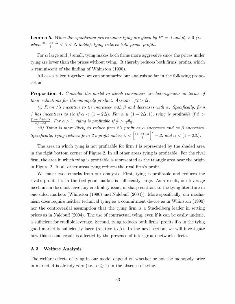
Proposition 4. Consider the model in which consumers are heterogenous in terms oftheir valuations for the monopoly product. Assume 1=2 > �.

(i) Firm 1�s incentive to tie increases with � and decreases with �. Speci�cally, �rm

1 has incentives to tie if � < (1 � 2�): For � 2 (1 � 2�; 1); tying is pro�table if � >(1��)2+4��4(1��) : For � > 1; tying is pro�table if �

�> �

1�� :

(ii) Tying is more likely to reduce �rm 2�s pro�t as � increases and as � increases.

Speci�cally, tying reduces �rm 2�s pro�t unless � <h(1��)+�

3

i2�� and � < (1� 2�).

The area in which tying is not pro�table for �rm 1 is represented by the shaded area

in the right bottom corner of Figure 2. In all other areas tying is pro�table. For the rival

�rm, the area in which tying is pro�table is represented as the triangle area near the origin

in Figure 2. In all other areas tying reduces the rival �rm�s pro�t.

We make two remarks from our analysis. First, tying is pro�table and reduces the

rival�s pro�t if � in the tied good market is su¢ ciently large. As a result, our leverage

mechanism does not have any credibility issue, in sharp contrast to the tying literature in

one-sided markets (Whinston (1990) and Nalebu¤ (2004)). More speci�cally, our mecha-

nism does require neither technical tying as a commitment device as in Whinston (1990)

nor the controversial assumption that the tying �rm is a Stackelberg leader in setting

prices as in Nalebu¤ (2004). The use of contractual tying, even if it can be easily undone,

is su¢ cient for credible leverage. Second, tying reduces both �rms�pro�ts if � in the tying

good market is su¢ ciently large (relative to �). In the next section, we will investigate

how this second result is a¤ected by the presence of inter-group network e¤ects.

A.3 Welfare Analysis

The welfare e¤ects of tying in our model depend on whether or not the monopoly price

in market A is already zero (i.e., � � 1) in the absence of tying.

33

Figure 2: Incentives to Tie in Two-Sided Markets

34

Case 1. (Full Market Coverage Case without Tying) � � 1For � � 1; the price in market A is zero and all consumers enjoy the service without

tying, which is an e¢ cient outcome. The equilibrium in market B is also e¢ cient without

tying because all consumers use the more e¢ cient service provided by �rm 2. Therefore,

tying can only reduce social welfare. From Proposition 4, we know that for � � 1, �rm 1

has incentives to engage in tying only for the parameter values such that the post-tying

equilibrium prices are characterized by eP � = 0; ep�2 = 0 (see Figure 2). In this case, thereare two sources of ine¢ ciencies. First, any consumer whose valuation in market A is less

than � purchases from �rm 2 and consumes only product B. Second, consumers whose

valuation in market A is more than � ine¢ ciently switch from �rm 2�s more e¢ cient

product to the bundled product. Note that consumer surplus increases in this case due to

a decrease in the price of �rm 2�s product from � to zero. Consumers whose valuation in

market A is more than � (u > �) are indi¤erent between the two regimes, but low type

consumers in market A (whose u < �) gain with tying because their utility is v2 with

tying while it was u+ v1 without tying.

Case 2. (Partial Market Coverage Case without Tying) � < 1When � < 1; the price in market A is positive without tying and the market outcome

is ine¢ cient whereas the market outcome in B is e¢ cient. As in the previous case, tying

can introduce ine¢ ciency in market B when �rm 1 ine¢ ciently serves consumers with a

bundled product, but there can be a positive market expansion e¤ect in market A as the

bundle price is reduced. As a result, social welfare can be ambiguous. However, for social

welfare to increase with tying a necessary condition is that market A expands with tying.

The next lemma derives the condition under which market A expands with tying.

Lemma 6. Market A expands with tying if and only if � < 1� 2�:

The immediate corollary of lemma 6 is that tying decreases social welfare if � > 1�2�:Now let us consider the case where � < 1 � 2� and hence market A expands with

tying. More generally, the social welfare change with tying (�W ) in this case can be

written as

�W =

Z 1��2

1� eD1(u+ �)du| {z }Welfare Gain in Market A

due to Market Expansion

� eD1�|{z}Social Welfare Loss in Market B

;

35

where eD1 denotes the demand for the bundle after tying. After analyzing the welfare

e¤ects of tying depending on the equilibrium price con�gurations (see the proof of Propo-

sition 5), we �nd that tying increases welfare for� small enough as in this case the welfare

loss in market B is small.

Proposition 5. Tying is welfare-reducing if � > 1 � 2� since market A contracts and

there is ine¢ cient switching in market B. If � < 1 � 2�; market A expands and tying

can enhance welfare if � is su¢ ciently small since ine¢ ciency associated with tying in

market B becomes arbitrary small as �! 0:

B Heterogenous consumers with intergroup network e¤ects

Up to now, we assumed two-sided markets in which the consumer side serves as a compet-

itive bottleneck but did not derive any direct utilities (or disutilities) from the other side

which can be considered as advertisers. This was to capture the advertising revenue-based

business model of many Internet platform markets such as Google. In this section, we ex-

tend our analysis by explicitly considering intergroup network e¤ects from the other side

to consumers. For instance, we can interpret the other side as app producers or content

providers. In the presence of network e¤ects, consumers� choices can exhibit strategic

complementarity and coordination plays an important role. In such a situation, tying can

be used as a strategic instrument to help consumers coordinate and coalesce around the

bundled product. We investigate how the presence of network e¤ects a¤ects the previous

results on the relationship between the incentive to tie and � (and �).

For simplicity, we assume that the monopolistic platform market A is the same as in

Section A. We modify market B as follows. Let pci be the price charged by platform i on

the consumer side in market B. Then, a consumer subscribing to platform i in market B

derives a utility of

vi + �cnai � pci ;

where �c(> 0) is a parameter representing intergroup network e¤ects and nai is the mea-

sure of applications/content available at platform i. We assume � � v2 �v1 > 0. On

the application side, let pai be the price an application developer needs to pay to have

access to consumers on platform i. An application developer�s payo¤ from developing an

application or creating content for platform i is

36

�anci � pai ;

where �a > 0 and nci is the measure of consumers on platform i. Marginal costs of serving

consumers are once again assumed to be zero.

We consider the following sequential game.

1. Each �rm (i.e., platform) sets the prices for consumers.

2. Consumers make purchase or subscription decisions

3. (After observing consumer choices at stage 2), each platform chooses the price for

application developers

4. (After observing consumer choices at stage 2 and price choices at stage 3), applica-

tion developers choose subscription decisions.

Stages 1 and 2 of this sequential game are identical to the games we studied in the

previous sections. The main di¤erence is that the advertising revenue per consumer in

market B was exogenously given in the previous sections whereas its equivalent is now

endogenous: solving for Stages 3 and 4 allows us to compute the additional pro�t that

a platform can obtain from the application side by attracting one more consumer. We

assume that consumers single home while application developers can multihome. As usual,

we analyze the game by using backward induction.

B.1 Equilibrium on the Application Side

Suppose that platform i has nic measure of consumers on board. Let us study the game

that starts at stage 4.

In order to endogenously derive the number of applications available, we assume that

each developer incurs a platform-speci�c �xed cost f . The �xed cost is distributed over

the positive line with density equal to one. Given the heterogeneity in the �xed cost

of development, an application developer will subscribe to platform i if the following

condition holds:

�anci � pai � f:

Hence, given nci and pai , the total measure of app developers who subscribe to platform i

is

nai (pai ;n

ci) = �an

ci � pai :

Therefore, at stage 3 with nai determined in the previous stage, platform i solves the

37

following problem.

maxpaipai n

ai (p

ai ;n

ci) = p

ai (�an

ci � pai ):

From the �rst-order condition for platform i�s pro�t maximization, platform i chooses

pai =�an

ci

2:

The measure of app developers who subscribe to platform i also is given by nai =�an

ci

2with

a uniform distribution of f with density one. As a result, given the number of consumers

nci ; platform i�s pro�t on the application side is

�ai (nci) =

��an

ci

2

�2:

Note that this result does not depend on whether or not there is tying on the consumer

side.

B.2 Equilibrium on the Consumer Side

We now analyze the e¤ects of tying on the consumer side.

B.2.1 No Tying

Consider platform competition at stage 1 without tying. As we assume that all consumers

are homogenous in market B, there can potentially be multiple equilibria for some price

con�gurations due to positive intergroup network e¤ects. In such cases, we assume that

all identical consumers coordinate on the Pareto dominant equilibrium.33

Hence, if pc2 < pc1+�, all consumers coordinate on platform 2 as long as their individual

rationality constraint is satis�ed. Therefore, in equilibrium, we have pc1 = 0; pc2 = � and

all consumers join the more e¢ cient platform 2, that is, nc1 = 0 and nc2 = 1. In this

tipping equilibrium with nc2 = 1, �rm 2 charges pa2 =�an

c2

2= �a

2on the application side

and induces a measure of na2 =�a2application developers to be on its platform. Thus,

each consumer�s payo¤ on platform 2 is

v2 + �cna2 � pc2 = v2 + �c

��a2

��� = v1 + �;

33This is a standard equilibrium selection criterion in the presence of multiple equilibria with networke¤ects. See, for instance, Katz and Shaprio (1986) and Waldman (1993).

38

where � � �c�a2represents the network bene�ts in the tipping equilibrium. As in the

analysis of the previous section, each consumer receives a surplus of v1 due to platform

competition on the consumer side. In addition, each consumer receives additional bene�t

of � = �c�a2from intergroup network e¤ects.

B.2.2 Tying

Now consider the equilibrium in the tying regime in which platform 1 ties its monopolized

product A with another product in competitive two-sided market B, and charges eP for

the bundled product. We make the following assumption:

Assumption 1. (stability) �c�a < 1, � < 1=2

Without this assumption, there cannot exist any interior equilibrium in which both

platforms share the market in our two-sided market. This is because the feedback mech-

anism due to intergroup network e¤ects magni�es any initial advantage of one platform

and leads to exploding demands.

We further assume that � < 1=2 for tying to have a leverage e¤ect in the tied good

market. If � is too large (i.e., � > 1=2), the disadvantage of �rm 1 vis-à-vis �rm 2 is

too large to overcome in the tied good market; tying has no leverage e¤ect. Note that

� < 1=2 along with the stability assumption implies that purchasing the bundle is the

dominant strategy for the highest consumer type in market A (whose u = 1) if the bundle

is o¤ered for free. For this type of consumer, the valuation of product A is so high that

the bundled product is preferred even if all other consumers purchase stand-alone product

B2 and there are no application developers for B1.

Therefore, in what follows, by using iterated elimination of dominated strategies, we

study a cut-o¤ equilibrium: we consider a u� 2 [0; 1] such that all consumers whose

valuation from the monopoly product is higher than u� join platform 1 while all the

rest join platform 2, which implies that nc1 = 1 � u�; nc2 = u� on the consumer side andna1 =

�a2(1� u�); na2 =

�a2u�:

Let eP and ep2 be the bundle price by �rm 1 and �rm 2�s price for product B2 in the

tying regime, respectively. In the (interior) cut-o¤equilibrium, u� is implicitly determined

as follows:

[u� + v1] + �(1� u�)� eP = v2 + �u� � ep2: (3)

The LHS of (3) represents type u� consumer�s utility when he purchases the bundled

product whereas the RHS of (3) represents type u� consumer�s utility when he purchases

39

only product B supplied by �rm 2. The critical type u� is indi¤erent between these two

options. Hence,

nc2(eP ; ep2) = u� = ( �+ eP�ep2��

(1��c�a); if eP > ep2 + � ��;

0; if eP � ep2 + � ��:The expression for nc2 above reveals new e¤ects of tying in the presence of intergroup

network e¤ects. If there are no network e¤ects (i.e., �c�a = 0), �rm 2 can always

guarantee a positive market share unless its price does not exceed the bundle price by

�. For instance, if �rm 2 charges a price of zero, �rm 2 will always have some positive

market share (nc2 > 0). However, because of the existence of network externalities (i.e., as

the number of consumers who choose platform 1 increases, the applications available on

that platform increases), tying can create an advantage for platform 1 if tying provides

a mechanism for �rm 1 to capture more consumers than �rm 2. As the network e¤ects

term (�c�a) increases, �rm 2�s market share decreases down to zero and eventually tying

leads to the foreclosure of �rm 2 in the market. Note that @nc2@ eP =

���@nc2@ep2��� = 1

1��c�a> 1 is

a multiplier in the two-sided market. It shows that the demand changes more sensitively

to price as �c�a increases.

Consider the case where nc2( eP ; ep2) > 0. Then, we can decompose the market share ofthe tying �rm into two terms as follows:

nc1( eP ; ep2) = 1�nc2( eP ; ep2) = 1�h( eP � ep2) + �i| {z }

Demand in the Absence of

Intergroup Network E¤ects

+�c�a

(1� �c�a)

�1

2�h( eP � ep2) + �i�| {z }

Induced Demand Due to

Intergroup Network E¤ects

;

(4)

where 1�h( eP � ep2) + �i is a hypothetical demand for �rm 1 in the absence of intergroup

network e¤ects (i.e., �c�a = 0), which we have seen in Section A (see equation (2)).

In order to understand equilibrium pricing, it is useful to decipher the economic

meaning of � 1 � �c�a �(�a)

2

2. As �rm 1�s pro�t under tying is given by e�1 =h eP + �+ (�a)

2nc14

inc1, its �rst-order condition for pro�t maximization is given by:

@e�1@ eP =

@nc1

@ ePh eP + �� nc1i = 0;

40

where @nc1@ eP = � 1

1��c�a. We can rewrite the condition above in a modi�ed Lerner index

form: eP + �eP =nc1eP :

If the tying �rm did not take into account the e¤ect of its bundle pricing decision on

the pro�t from the application side, would not contain the term (�a)2

2and we would

have = 1 � �c�a, which is equal to the inverse of���@nc1@ eP���. Therefore, we can state the

�rst-order condition as the standard Lerner formula with the interpretation of (��) as theopportunity cost of the bundle. corrects the standard formula by taking into account

the fact that an increase in market share increases the pro�t from the application market

through the network e¤ects. If this e¤ect is large such that � 0, �rm 1 �nds it optimalto choose eP = 0 for any � � 0. The same remark applies to �rm 2. Therefore, � can beconsidered a measure of degree of competition induced by intergroup network e¤ects, which

increases with the network e¤ects and the pro�t per consumer from the app market.

We can have two types of equilibria: an interior equilibrium in which �rm 1 and �rm 2

share the market with nc2 > 0 and the tipping equilibrium in which the tying �rm captures

the whole market with nc2 = 0.34 The following proposition characterizes the equilibrium

conditions.

Proposition 6. We have a tipping equilibrium (with nc1 = 1 and nc2 = 0) if � � � and

� � b� � (� � �) + , where = 1 � �c�a �(�a)

2

2: Otherwise, we have an interior

equilibrium with both nc1 > 0 and nc2 > 0:

In the proofs for online publication material, we not only prove the proposition above

but also further characterize equilibrium prices in each type of equilibrium. Proposition 6

shows that if � > �, that is, the quality advantage of �rm 2 is su¢ ciently large compared

to the strength of network e¤ects, we always have an interior equilibrium. However, if the

network e¤ects are relatively stronger than the quality advantage of �rm 2 (i.e., � < �),

tying can be a mechanism for �rm 1 to leverage its market power in A to B and lead

to foreclosure of the rival �rm. Note that the condition for tipping is more likely to be

satis�ed as � increases. For instance, if � > 1, we always have a tipping equilibrium as

long as � < �:

34With the maintained assumption of � < 1=2 and the stability assumption, there is no tippingequilibrium in which �rm 2 captures the whole market.

41

B.3 Incentives to Tie with Intergroup Network E¤ects

We now analyze incentives to tie in the presence of intergroup network e¤ects. Proposition

6 shows that when � � � holds, a tipping equilibrium is more likely as � increases. This

is because a high � induces the monopolist to price more aggressively in the consumer

market, providing more surplus to inframarginal consumers, which can be leveraged to

attract all consumers in market B through network e¤ects (see the demand decomposition

in (4)). If tipping occurs, �rm 1 captures all advertising revenue in market A, which breaks

the result obtained in the previous section that there exists a critical value of �� such that

tying is not pro�table if � � ��.

B.3.1 Tipping Equilibrium

As shown in Proposition 6, we have a tipping equilibrium if � � � and � � 1� [(�c�a +(�a)

2

2)+(���)]: In the tipping equilibrium, p� = 0, P � = ���. Thus, �rm 1�s pro�t with

tying is e��1 = �+��a2 �2+(���) while its pro�t without tying is ��1 =max�14(1 + �)2; � :When � � 1, �rm 1 serves all consumers in the tying market regardless of tying. Therefore,tying is pro�table as it increases the pro�t from the tying market from � to � + � � �and generates the pro�t from the apps. By continuity, tying is pro�table for � close to

one and we have the following result.

Proposition 7. When the tipping equilibrium prevails under tying, �rm 1 has incentives

to tie if � > �� � 1�q(�a)

2 + 4(� ��):

Proof. When � � 1, �rm 1�s pro�t without tying is �: Since �c�a2� � in the tipping

equilibrium, it immediately follows that tying is pro�table when � � 1: For � < 1, �rm1�s pro�t under tying is 1

4(1 + �)2: A simple comparison of �rm 1�s pro�ts under each

regime yields the result.�The proposition indicates that tying is more likely to be pro�table for � high, �c high

and �a high. Propositions 6 and 7, taken together, yield the following Corollary.

Corollary 1. If � � � and � > max[b�; ��] (where max[b�; ��] < 1), �rm 1 engages in

tying and the resulting equilibrium is a tipping equilibrium in which �rm 2 is foreclosed

from the market.

We point out the di¤erence the introduction of intergroup network e¤ects creates with

respect to the result in the previous section. In section A, for a given �; tying becomes

42

unpro�table at some point as � increases. The reason is that without network e¤ects,

the rival �rm can always induce some marginal consumers in market A to buy product

B when tying takes place. As a result, tying entails greater loss as � increases. However,

this e¤ect can disappear in the model with intergroup network e¤ects if tying induces a

tipping equilibrium, which is more likely when � is high.

B.3.2 Interior Equilibrium

Due to the con�icting e¤ects of �, the e¤ects of tying on the tying �rm�s pro�ts can be

subtle in the interior equilibrium. As explained earlier, a higher � induces the tying �rm to

price more aggressively in the consumer market, providing more surplus to inframarginal

consumers of A, which can be used to compete against �rm 2 in market B when tying

takes place. In the interior equilibrium, however, capturing a certain share of market B

comes at the expense of the share of market A, which can be very costly when � is very

high. We thus can show that tying cannot be a pro�table strategy if � is su¢ ciently large

as in Section A.

In the case of an interior equilibrium, let us focus on the case in which eP � = 0. Thisholds either if < 0 and � < � (see Lemma 7(ii) in the proofs for online publication

material) or if � 0 but nc�1 is bounded above by � (i.e. (6) is satis�ed) (see Lemma9(i) in the proofs for online publication material). In both cases, �rm 1�s market share

under tying is independent of � and is given by

nc�1 =

(1� ���

(1��) if < 0;

1� ���+(1��) if � 0.

De�ne the di¤erence between �rm 1�s pro�t under tying and �rm 1�s pro�t without tying

as follows

��(�) �(nc�1 (�+

(�a)2

4nc�1 )�

�1+�2

�2; if � 2 [0; 1] ;

nc�1 (�+(�a)

2

4nc�1 )� �, if � > 1:

Suppose that nc�1 is close enough to one that��(1) > 0. Note �rst that��(�) is concave

for � 2 [0; 1]. For � > 1, as ��(�) linearly decreases, there exists � = (�a)2

4nc�1 =(1� nc�1 )

at which��(�) = 0. We below distinguish the case of��(0) � 0 from��(0) < 0. Sup-pose ��(0) � 0. Then, tying is strictly pro�table for any � 2 (0; �). If ��(0) < 0, thereexists some �2 (0; 1) at which ��(�) = 0. Hence, tying is pro�table for any � 2 (�; �).As � tends to 1 when nc�1 goes to one, the result obtained when ��(0) < 0 extends the

43

result on the incentive to tie in the tipping equilibrium, described in Proposition 7, to an

interior market share.

B.4 Welfare Analysis

We now analyze welfare implications of tying. First consider the case where tying leads

to tipping. If � > 1, all consumers in market A were served before tying. There is

thus no market expansion e¤ect in this case. The only e¤ect is that consumers switch

from �rm 2�s product to �rm 1�s product, which is inferior. Thus, tying unambiguously

reduces welfare in this case, with the welfare loss being �: If � < 1, but tying induces

tipping, there is a positive market expansion e¤ect in market A. The welfare gain from

this market expansion can be expressed as

E =

Z 1��2

0

udu+

�1� �2

�� =

(1 + 3�)(1� �)8

This welfare gain needs to be measured against the loss in welfare in market B, which

is �: Tying can be welfare reducing if E < �: E is highest at 1=6 when � = 1=3:

Therefore, a su¢ cient condition that tying reduces welfare is � > 1=6 if tying induces

tipping towards the bundled product.

If tying does not lead to tipping, there is an additional type of welfare loss due to a

fragmented market structure which does not fully exploit network bene�ts.

We can also analyze the e¤ects of tying on consumer surplus. For instance, suppose

that � > 1 and tying leads to tipping. If eP � = 0, consumers are indi¤erent between

tying and no tying. However, if eP � > 0, consumers lose from tying. Without tying, each

consumer enjoys (�a)2

2of surplus from �rm 2 in market B because of price competition in

market B. Tying removes the level playing �eld and allows the tying �rm to extract the

surplus from network e¤ects.

Proofs for Online Publication Material

Proof of Lemma 1

(i) If eP 2 [ep2 ��; 1 + ep2 ��], �rm 1�s pro�t is

�1( eP ; ep2) = (1� [( eP � ep2) + �])( eP + �+ �)44

The �rst-order condition with respect to eP is equivalent toeP = (1��)� (�+ �) + ep2

2:

For this to be the optimal, the condition eP = (1��)�(�+�)+ep22

� maxf0; ep2 ��g needs tobe satis�ed.

When 0 � eP < ep2 ��, �rm 1�s pro�t is

�1( eP ; ep2) = ( eP + �+ �)Hence, it is optimal to choose eP = maxf0; ep2��g given the non-negative price constraint.Therefore, the best response is eP = (1��)�(�+�)+ep2

2for � + [1� (�+ �)] � ep2 >

� � [1� (�+ �)]. If 1 � � + � or for ep2 =2 [� + [1� (�+ �)] ;� � [1� (�+ �)], it isoptimal to choose eP = maxf0; ep2 ��g.(ii) Firm 2�s pro�t is zero if 0 � eP < ep2 ��: If eP � ep2 ��, its pro�t is

�2( eP ; ep2) = [( eP � ep2) + �](ep2 + �):The �rst-order condition with respect to ep2 yields

[( eP � ep2) + �]� (ep2 + �) = 0;which can be rewritten as ep2 = (�� �) + eP

2:

For this to be the optimal, the condition for ep2 = (���)+ eP2

� eP +� needs to be satis�ed,

i.e., eP � �(� + �);which holds always. We can thus write the best response of �rm 2 as

BR2( eP ) = max[(�� �) + eP2

; 0]

Proof of Lemma 2

It is omitted as it is straightforward from the explanations in the main text.

Proof of Lemma 3

45

In this case, it can be easily shown that eP � > ep2�: Thus, the non-negative priceconstraint is binding �rst for the rival �rm�s price under tying. We thus have

eP � = (1��)� (�+ �)2

; ep�2 = 0:Firm 1 and �rm 2�s demands are respectively given by

eD1 =(1��) + (�+ �)

2; ed2 = (1 + �)� (�+ �)

2:

The corresponding pro�ts are given by

e�1 = �(1��) + (�+ �)2

�2; e�2 = � �(1 + �)� (�+ �)

2

�:

Since � < 1�2� in the case we consider, �rm 1�s pro�t under no tying is �1 =�1+�2

�2:

Since � > � in this case, we have e�1 > �1, that is, tying is pro�table for the tying �rm.In contrast, tying reduces the rival �rm�s pro�t. To see this, note that the rival �rm�s

pro�t in the absence of tying is �2 = � + � > � > �h(1+�)�(�+�)

2

i= e�2 because

(1 + �)� (�+ �) < 2 as � > �:

Proof of Lemma 4

It is omitted as the proof of (i) and (ii) is provided in the main text and the proof of

(iii) is straightforward.

Proof of Lemma 5

In this case, it can easily be shown that eP � < ep2�: Thus, the non-negative priceconstraint is binding �rst for the tying �rm We thus have

eP � = 0; ep�2 = �� �2

:

Firm 1 and �rm 2�s demands are respectively given by

eD1 = 1��+ �

2; ed2 = �+ �

2:

46

The corresponding pro�ts are given by

e�1 = (�+ �) �1� �+ �2

�; e�2 = ��+ �

2

�2:

We need to show that

e�1 = (�+ �) �1� �+ �2

�<

( �1+�2

�2if � < 1

� if � > 1

For � < 1;we use the following fact�x+ y

2

�2� xy for any x and y:

Let x = �+ � and y = 1� �+�2: Then, we have

(�+ �)

�1� �+ �

2

�<

�2 + 2�+ � ��

4

�2:

Since � < � in this case, we have�2+2�+���

4

�2<�1+�2

�2: Therefore, e�1 = (� +

�)�1� �+�

2

�<�1+�2

�2= �1 if � < 1:

For � > 1; tying is pro�table only when (�+�)�1� �+�

2

�> �: This condition can be

rewritten as

� <2�

�+ �� �:

Since � < �, the condition above can be satis�ed only when � < 2��+�

��, or (�+�) < 1;which is impossible because � > 1: Therefore, tying cannot be pro�table for � > 1, either.

Tying obviously hurts �rm 2 as tying reduces its price and market share.

Proof of Lemma 6

In market A, all consumers whose valuations satisfy u � 1��2purchase product A.

With tying, all consumers whose valuations satisfy u � (1 � eD1) consume product A,

where eD1 denotes the bundle demand for �rm 1. Thus, for market A to expand we need1��2> (1� eD1): We can easily verify that this condition is equivalent to � < 1 � 2� by

checking all possible equilibrium price con�gurations with tying.

47

Proof of Proposition 5

� eP � = 0; ep�2 = 0Consider a situation in which the post-tying equilibrium prices are zero ( eP � = 0; ep�2 =

0): Because eD1 = 1 �� in this case, the social welfare change with tying (�W ) can be

written as

�W =

Z 1��2

�

(u+ �)du� (1��)�

We can easily see that if � is su¢ ciently small, then social welfare loss in market B

from tying is negligible. Thus, if � is su¢ ciently large, �rm 1 has incentives to capture

market B with tying, and tying can be socially bene�cial as the market expansion e¤ects

in market A outweigh social welfare loss in market B.35

Consumer welfare in this case always increases because now both goods are provided

for free.

� eP � > 0; ep�2 = 0In this case, eD1 =

(1��)+(�+�)2

: By proceeding in a similar way as above, we can verify

that if � is su¢ ciently small, tying can increase welfare. Otherwise, tying decreases

welfare. It can also be shown that market A always expands with tying as 1��2> 1� eD1

in this case.

Concerning consumer welfare, we can easily verify that eP � = (1��)�(�+�)2

< pm = 1��2,

i.e., the bundled product is even cheaper than the stand-alone A product price before

tying. As a result, consumers bene�t from tying.

� eP � > 0; ep�2 > 0In this case, eD1 =

2+���3

: Once again, if � is su¢ ciently small, tying can increase

welfare. Otherwise, tying decreases welfare.

Proof of Proposition 635We can also show that if � > 1=7, tying reduces welfare regardless of the value of �:

48

To derive the equilibrium prices under tying, note that �rm 1�s and �rm 2�s total

pro�ts are respectively given by

e�1( eP ; nc1( eP ; ep2)) = ( eP + �)nc1 + ��an

c1

2

�2| {z }

Pro�t from the App Side

;

e�2(ep2; nc2( eP ; ep2)) = ep2nc2 + ��anc22�2

Firm 1�s �rst-order condition for pro�t maximization is given by

@e�1@ eP = nc1 +

" eP + �+ (�a)2 nc12

#@nc1

@ eP= � 1

1� �c�a

" eP + �� nc1(1� �c�a � (�a)22 )

#

where @nc1@ eP = � 1

1��c�a(= �@nc2

@ eP ): Using � 1��c�a� (�a)2

2, we can rewrite the expression

above as@e�1@ eP = � 1

1� �c�a

h eP + �� nc1i :If < 0, we always have @e�1

@ eP < 0, implying that eP = 0 is optimal in the interior

equilibrium where nc2 > 0. In a tipping equilibrium with foreclosure where nc2 = 0, there

is no market share to gain and hence it is not optimal to reduce the price further and we

will have eP = ep+ (� ��).Similarly, �rm 2�s �rst-order condition for pro�t maximization is given by

@e�2ep2 = nc2 +

"ep2 + (�a)2 nc22

#@nc2ep2

= � 1

1� �c�a[ep2 � nc2]

where @nc2@ep2 = � 1

1��c�a. Once again, if < 0, we have @e�2ep2 < 0, implying that ep2 = 0 is

optimal.

Note that the second-order derivatives for �rm 1 and �rm 2 are the same and given

49

by:@2e�1@ eP 2 = @2e�2

@ep22 = � 1

1� �c�a�"1� (�a)

2

2

1

1� �c�a

#1

1� �c�a:

They are negative if

(�a)2 < 4 (1� �c�a) ;

which is equivalent to

�c�a +1

4(�a)

2 < 1:

We consider two cases depending on the magnitudes of intergroup externality para-

meters (i.e., the sign of ).

Case 1. < 0 (i.e., �c�a +(�a)

2

2> 1)

In this case, the equilibrium prices are ep�2 = 0 and eP � = max f0; � ��g as @e�2ep2 < 0: Wecan have two types of equilibria depending on the relative magnitude of � and�: a tipping

equilibrium or an interior equilibrium. We have the following lemma that characterizes

equilibrium in this case.

Lemma 7. Suppose that < 0: Then, we have ep�2 = 0.(i) If � > �; we have a tipping equilibrium in which nc�2 = 0 and eP � > 0.(ii) If � < �, we have an interior equilibrium with nc�2 > 0 and both prices being driven

down to zero ( eP � = ep�2 = 0), wherenc�2 =

�� �(1� �c�a)

> 0;

nc�1 = 1� nc�2 =1� (� + �)(1� �c�a)

> 0:

Case 2. � 0 (i.e., �c�a +(�a)

2

2� 1)

We also consider two types of equilibria under tying in this case: a tipping equilibrium

and an interior equilibrium. Note that in this case (i.e., when � 0); the second-ordercondition is always satis�ed in each �rm�s maximization problem.

Tipping Let us �rst analyze the possibility of a tipping equilibrium. In a tipping

equilibrium with nc�2 = 0; we have the following �rst-order condition for �rm 2:

@e�2ep2 = � ep21� �c�a

� 0:

50

Hence, ep�2 = 0. Then, the highest eP consistent with tipping is eP � = max f0; � ��g.At this price, �rm 1 must have no incentive to deviate; the �rst-order derivative must be

zero or negative.

If � < �; the equilibrium prices in a tipping equilibrium need to be eP � = ep�2 = 0:

However, at these prices �rm 2 has a strictly positive market share. We thus have a

contradiction and there cannot be a tipping equilibrium if � < �:

If � � �; then eP � = � �� and the following condition must hold:

@e�1eP = � 1

1� �c�a[� ��+ ��] � 0;

which is equivalent to

� � (�� �) + :

Summarizing, we have:

Lemma 8. Suppose that � 0. There is a tipping equilibrium in which eP � = � �� �p� = 0 if � � � and � � (�� �) + , where = 1� �c�a �

(�a)2

2:

Interior Equilibrium Let us look for an interior equilibrium (i.e., each �rm has a

positive market share): 0 < nc�2 < 1. For an interior equilibrium, �rm 2�s �rst-order

condition for pro�t maximization is given by

ep�2 = nc�2 > 0: (5)

However, eP � can be zero. From �rm 1�s �rst-order condition, we have:

eP � = max f0;��+ nc�1 g :Consider the case of eP � = 0: Then, from the demand function and (5), we have

nc�2 =(�� �)� nc�2 (1� �c�a)

By collecting terms in nc�2 , we have

nc�2 =�� �

+ (1� �c�a):

51

eP � = 0 is an equilibrium price for �rm 1 if

nc�1 � �;

which is equivalent to �1� �� �

+ (1� �c�a)

� � �: (6)

If (6) is violated, then eP � = ��+ nc�1 > 0:Then, eP � � ep�2 = (1� 2nc�2 )� �:Putting this into the market share equation leads to

nc�2 (1� �c�a) = (�� �) + (1� 2nc�2 )� �;

which can be rewritten as

nc�2

"3 +

(�a)2

2

#= (�� �)� �+:

Therefore,

nc�2 =(�� �)� �+3h+ (�a)

2

6

i=

32

h+ (�a)

2

6

i� 1

2+�� �

3h+ (�a)

2

6

i=

1

2� 1 + 2�� 2�6 + (�a)

2

Hence, �rm 1�s market share is

nc�1 = 1� nc�2 =1

2+1 + 2�� 2�6 + (�a)

2 :

Because we assume = 1 � �c�a �(�a)

2

2> 0, the denominator in the market share

52

expression is strictly positive. Under the maintained assumption of � < 1=2, �rm 1�s

market share is larger than 1=2, which is the market size in the monopolized market

A without tying when it is one-sided (i.e., when � = 0). The market share for �rm 1

increases with � and decreases with �, as expected. The market share�s response to � or

� is greater as the intergroup externalities in market B becomes more important (i.e., as

�c or �a increases).

Firm 1�s equilibrium price is

eP � = ��+ nc�1 � 0:

= ��+ 2+(1 + 2�� 2�)6 + (�a)

2 :

We �nd

@ eP �@�

= �1 + 2

6 + (�a)2

2

= �4 + (�a)2

6 + (�a)2 < 0:

@ eP �@�

< 0:

@ eP �@�c

= nc�1@

@�c+ � @n

c�1

@�c

= ��a�1

2+1 + 2�� 2�6 + (�a)

2

�+ � �a

1 + 2�� 2�

6h+ (�a)

2

6

i2= ��a

2412+1 + 2�� 2�6h+ (�a)

2

6

i "1�

+ (�a)2

6

#35 < 0:Firm 2�s equilibrium price is

ep�2 = nc�2

=

�1

2� 1 + 2�� 2�6 + (�a)

2

�:

For a given market share, �c�a > 0 induces �rm 2 to charge a lower price to consumers

53

for product B than when �c�a = 0. In addition, as long as 1 + 2� � 2� > 0, �rm 2�s

market share is smaller when �c�a > 0 than when �c�a = 0. Hence, both factors would

induce �rm 2 to become more aggressive.

Summarizing, we have:

Lemma 9. Suppose that � 0 and the conditions for the tipping equilibrium in Lemma

8 are not met. Then, there is an interior equilibrium such that

(i) if (6) is satis�ed, eP � = 0, ep�2 = nc�2 > 0 andnc�2 =

�� �2 + (�a)

2

2

:

(ii) if (6) is violated, eP � = ��+ (1� nc�2 ) > 0; ep�2 = nc�2 > 0 andnc�2 =

1

2� 1 + 2�� 2�6 + (�a)

2

All the results in lemmas 7-9 we derived under di¤erent parameter con�gurations can

be summarized as in Proposition 6.

54