a literature review of the numerical simulation of mixers, s.s.e., and t.s.e. (1994-2003), part...
TRANSCRIPT
D E P A R T M E N T O F M E C H A N I C A L E N G I N E E R I N G
A . J A M E S C L A R K S C H O O L O F E N G I N E E R I N G
Center for Energetic Concepts Development
A Literature Review of the Numerical Simulation of Mixers, S.S.E., and T.S.E. (1994-2003)
Part 1
B. BergerEmeritus Professor
Department of Mechanical Engineering2181 Glenn L. Martin Hall
University of MarylandCollege Park, MD 20742Telephone: 301-405-5262Facsimile: 301-314-9477
E-Mail: [email protected]
December 20, 2004

INTRODUCTION A preliminary attempt has been made here to survey the state of the art in the computer
simulation of flows in T.S.E.. Twenty-two publications spanning the period 1994-2003, dealing
specifically with the numerical simulation of flow in 2 and 3-D mixers, single and twin screw
extruders, have been reviewed. The inclusion of mixers and S.S.E. was predicated on the
observation that algorithms developed for the analysis of these simpler geometrics have often
been generalized effectively for the analysis of T.S.E..
A summary, in tabular form, listing essential reference data is provided for rapid reference.
A brief section of conclusions follows. Individual reviews, grouped according to algorithm, and
mixer geometry are then presented.
Although the review is not exhaustive, an effort has been made to include recent publications
of comprehensive F.E.M., B.E.M. and D.R.B.E.M. algorithms. The encouragement of Professor
D. K. Anand is appreciated. Typing of the manuscript was expertly executed by L. Crittenden.
1

SUMMARY
The following summary tabulates only essential data drawn from the references, where
T.S.E. = twin screw extruder, F. B. = full barrel, TEMP. = temperature calculation, F.E.M. =
finite element method, G. N. = generalized Newtonian fluid, B.E.M. = boundary element
method, C. F. = creeping flow, N = Newtonian fluid, G. N. S. = generalized Newtonian fluid
with solids loading, F.A.N. = flow analysis network, S.B. = starved barrel, MIX = mixer, F =
fluid, F.A.T. = full acceleration term, T. D. = time dependent, D.R.B.E.M. = dual reciprocity
boundary element, C. D. = circular drop, P. F. = partially filled, R. C. F. = reacting creeping
flow, V. E. = visco-elastic fluid.
Ref. No.
[1] T.S.E., F.B., 3-D, F.E.M., TEMP., G.N., C.F.
[2] T.S.E., F.B., 3-D, F.E.M., TEMP., G.N., C.F.
[3] T.S.E., F.B., 3-D, F.E.M., TEMP., G.N., C.F.
[4] T.S.E., F.B., 3-D, F.E.M.,---------, N., C.F.
[5] T.S.E., F.B., 3-D, F.E.M.,---------, N., C.F.
[6] T.S.E., F.B., 3-D, F.E.M., ------, N., C.F.
[7] T.S.E., F.B., 2-D, F.E.M., TEMP., G.N.S., C.F.
[8] T.S.E., F.B., 2-D, F.A.N., ------, G.N., C.F.
[9] T.S.E., S.B., experimental, C.F.
[10] MIX, 1F, 2-D, D.R.B.E.M., TEMP., G.N., C.F.
[11] MIX, 1F, 2-D, DRBEM, TEMP., G.N., F.A.T.
[12] T.S.E., F.B., 2-D, B.E.M., -----, N., C.F.
[13] T.S.E., F.B., 2-D, B.E.M., ------, N., C.F.
2

[14] MIX, 2F, 2-D, B.E.M., ------, N., C.F.
[15] S.S.E., F.B., 3-D, B.E.M., ------, N., C.F.
[16] REVIEW ARTICLE
[17] REVIEW ARTICLE
[18] REVIEW ARTICLE
[19] C.D., 2F, 2-D, B.E.M., ------, N., F.A.T.
[20] T.S.E., F.B., 3-D, F.E.M., TEMP., G.N., R.C.F.
[21] MIX, P.F., 2-D, F.E.M., TEMP., G.N.S., C.F.
[22] MIX, 1F, 2-D, F.E.M., ------, V.E., C.F.
[23] 2-D flow of viscoelastic fluids with memory.
3

CONCLUSIONS
Conclusions drawn here are supported by the data presented in the summary. In some cases, reference is made to information contained in individual reviews.
From the summary it is seen that ref. [1-6, 20] report successful F.E.M. analysis of full barrel 3-D creeping flows in T.S.E. of Newtonian and generalized Newtonian fluids, reacting, and non-reacting.
These simulations were limited to short segments of full barrel T.S.E. and performed on relatively modest single processor workstations. Execution times for full size T.S.E. on possibly multi processor or vector machines are difficult to estimate.
In view of this, it appears that: 1. Already implemented F.E.M. algorithms for the creeping flow of a variety of fluid
models have been demonstrated which are applicable to full scale full barrel flows in T.S.E.
2. There is a possibility that through the use of large vector or parallel processors, (MIMD),
reasonable execution times, for these algorithms, could be achieved. Reference [20] reports on F.E.M., 3-D, solution for the flow of a chemically reacting
Newtonian fluid within a full barrel T.S.E.. References [7 and 21] discuss an F.E.M., 2-D, solution for the flow of a generalized Newtonian fluid with solids loading within a full barrel T.S.E. and a mixer, respectively. An F.E.M. solution for the 2-D flow of a viscoelastic fluid within a mixer is presented in [22].
From this it is reasonable to infer that: 3. Existing F.E.M. algorithms and codes could form the basis for the calculation of 3-D
flows within T.S.E. of viscoelastic fluids, generalized Newtonian fluids with solids loading, and chemically reacting Newtonian fluids. Such extensions would incur increased execution times.
As an alternative to F.E.M., B.E.M., the boundary element method, provides a
computational algorithm which is one dimension less than the corresponding F.E.M. formulation. In B.E.M., only domain boundaries are discretized. Ref. [12 and 15] present B.E.M. solutions for full barrel Newtonian, creeping, flows in a 2-D approx. of a T.S.E. and a 3-D simulation of a S.S.E., respectively.
These results suggest that: 4. Existing B.E.M. algorithms could form the basis for the calculation of 3-D, full barrel,
Newtonian flows, within T.S.E.. The resulting codes would reduce memory requirements and execution times.
References [10, 11] present analysis of the 2-D mixing of a generalized Newtonian fluid with
thermal effects for creeping flow and for the full acceleration term including products in the velocity, respectively. Nonlinearities appearing in both cases require the replacement of B.E.M. with the far more complex D.R.B.E.M.. In general, B.E.M. are more efficient than F.E.M.. However, when the necessity of using D.R.B.E.M. rather than B.E.M. arises, much of the
4

advantage of B.E. over F.E. is lost. It is shown in [10] that parallel processing on a 32 node connection machine reduces single processor execution times by factors of from 10-15.
These results suggest that: 5. D.R.B.E.M. solutions for the flow of generalized Newtonian fluids, with thermal effects
and including the nonlinear acceleration term, through full barrel T.S.E. is feasible provided execution time could be kept within reasonable limits, possibly through large scale parallel processing.
Ref. [14] presents a B.E.M. solution for the combined creeping flow of 2 distinct Newtonian
fluids in a 2-D mixer. The boundary between the fluids is computed and tracked as a function of time. The motion of an initially circular 2-D region of Newtonian fluid surrounded by a different Newtonian fluid, in the presence of a rigid no slip surface is computed through 2-D D.R.B.E.M. in Ref. [19]. Ref. [21] gives the creeping flow of a generalized Newtonian fluid with solids loading and temperature effects in a partially filled 2-D mixer.
From the foregoing it appears that: 6. Possible avenues of further research into the modeling of flows in the difficult case of
partially filled or starved T.S.E. are suggested by the approaches of Ref. [14, 19, 21]. 7. The results of Ref. [23] open up the possibility of constructing codes for the calculation
of flows of viscoelastic fluids with memory in T.S.E. based on the Newtonian fluid solution. Large Multiple Instruction Multiple Data computers with distributed memory would be essential for the associated computations.
5

Summary of Reference 1
In [1], the field and constitutive equations are ,0v =⋅∇ 0=⋅∇+∇− τp , , v:v 2 ∇+∇=∇⋅ τρ TkTC p Dητ 2= , ))(()( THFTH γη &= ,
DII2=γ& , , Carreau’s model, and 2/)1(20 )]2(1[ −+= n
dc IIF λη )](exp[)( 0TTTH −−= β . The solution is quasi-static, full barrel, no-slip, max. rotational speed = 420 r.p.m. Experimental verification of predicted pressure and temperature profiles is good. Velocity distributions are computed. 3-D, FEM Galerkin method applied to the flow field. Upwind Petrov-Galerkin applied to the
temperature field. The material is high density polyethylene. The measured temperature 200°C < T < 290°C. The modeled TSE is 2-stage. Only the rotor region of the second mixing stage was analyzed
over a length of 0.25m. The barrel diameter is 100mm. Mesh dimensions and computer execution times are not given.
Summary of Reference 2 Field and constitutive equations are identical to those of [1]. 3-D, FEM identical to [1]. Full
barrel of D=30mm. Modeled a TSE over 10 kneading discs for a total length of 9.3cm. In the flow field there were 22,561 nodes with 60,843 degrees of freedom. There were 20,281 degrees of freedom in the temperature field.
Computer used was an HP-J2240 without parallel processing. Execution time for each rotor position = 90 min. with 480MB of memory.
Exact specifications for the HP-J2240 were not available from H.P. An upper limit of 500 MHz was estimated by H.P. Desktop systems operating at 3.6GHz are available giving a ratio of 7.2:1. Improvements in memory access and internal information transfer probably boost this ratio to 10:1. Execution time for each rotor position would then ≅ 9 min.
6930 markers were defined in the simulation and followed in the evolution of the flow. The residence time distribution, nearest distance for each marker, and several mixing indices were studied.
The rotational speed = 60 r.p.m., and the material was probably high density polyethylene, quasi-static model.
Summary of Reference 3 Field and constitutive equations are identical to those of [1,2], except that
, Cross model. Full barrel, no-slip, barrel temp. = 200°C, max. rotational speed = 400 r.p.m.. 3-D, FEM similar to [1]. Studied a right-handed screw with left-handed slots, right-handed full flight screw and a right-handed full flight screw for a T.S.E. In all three cases 30mm of the T.S.E. was modeled. There were 42,470 nodes and 65,011 degrees of freedom in the flow analysis and 41,785 degrees of freedom in the temp. analysis. Computer
)))((/()( 10
nTHHTH −= γληη &
6
memory employed = 900MB and execution time = 60 min. per iteration on a Compaq Alpha Station DS20E.
The DS20E may be configured to run at 500, 667, or 833 MHz. Since the authors did not specify a configuration, for the purposes of estimation, assume 667MHz. Current desktop systems run at 3.6GHz. The speed ratio of the new to the old is 5.4:1, which is probably closer to 7:1 considering improvements in memory access and internal information transfer. Then on a current machine the solution for 3cm of a T.S.E. mixing element would require 8.6 min. for convergence after 5 iterations of each rotor position.
≅
As in [1, 2], the analysis is quasi-static and non-isothermal. The motion of 1778 massless marker particles was studied. Pressure, temperature, mixing coefficients, area stretch, max. values of the stress magnitude were found for the three screw geometries. The material studied was polypropylene. Computed results are in reasonable agreement with experimental results.
Summary of Reference 4 Field and constitutive equations are identical to those of [3] except that the flow is assumed
to be isothermal. The model is quasi-static with a no-slip boundary condition. The material is a low density polyethylene melt at 180°C. Max. rotational speed = 60 r.p.m.. The Galerkin F.E.M. method is employed with a 27 node tri-quadratic brick element for the components of the velocity vector. The pressure is found using a penalty function as follows:
)v( ⋅∇−= λp 0]))v()v[(()v( =∇+∇⋅∇+⋅∇ Tηλ
810=λ where ≡λ penalty number. Analyzed a set of 5 kneading discs each of width = 10mm. A mesh composed of 1344 elements with 13,543 degrees of freedom was used which introduced an error of less than 4% as compared with an analysis based on a mesh of 2352 elements. Execution times and storage requirements were not provided.
A total of 6930 markers were followed and the nearest distance between markers, average residence time and concentration of markers in the z-direction computed.
Summary of Reference 5 The fluid is modeled as an incompressible Newtonian fluid undergoing a 3-D isothermal
creeping flow. A 3-D T.S.E. is considered with pairs of two-tipped kneading discs staggered forward at various angles. Field equations are:
0v =⋅∇ v2η∇=∇p
3,1),,(vv == itxi The Galerkin F.E.M. method with a penalty function is used in the discretization with
)v( ⋅∇−= βηp and 610=β
7

The F.E. model consisted of 1280 tri-linear eight noded brick elements with a total of 1347 nodes at each axial section. For a 30° stagger angle, there are 25,600 brick elements, 28,287 nodes, and 84,861 degrees of freedom. The solution is quasi-static with a no-slip boundary condition and a full barrel.
Lyapunov exponents, residence times, Poincaré sections and tracer paths are found. Chaotic dynamics are indicated in the T.S.E. with two-tipped kneading discs. Computer memory requirements and execution times are not provided.
Summary of Reference 6 This is a generalization of [5]. The field equations are
0v =⋅∇ v2∇=∇ ηp
Again the penalty function is ( )v⋅∇= ηλpp
The no-slip boundary condition is assumed. The flow is quasi-static, isothermal and the fluid incompressible.
A 3.46” lead screw with a helix angle of 16.25 is modeled. The 3-D mesh had 10,920 elements, 12,432 nodes, 37,296 simultaneous equations and a global stiffness matrix with (22)·106 non-zero entries. Execution time was 73 min. per iteration on three parallel processors. Several iterations were required for convergence.
For screw geometrics in which the flight width is small in comparison to the channel width of the screw element, there is good agreement between the 3-D and 2-D models.
A Bingham fluid was used for which ( )( ) ( )( )⎥
⎦
⎤⎢⎣
⎡−−
−−+= −
011 exp
||||exp1
|| TTcn
m byn
γγτ
γη&
&&
T0 = entrance temp., dII=γ& , d = deformation rate tensor.
Summary of Reference 7 The analysis is based on a 2-D model of a T.S.E. The 2-D versions of the 3-D field
equations of [5, 6] are augmented with a solution of the energy equation based on the SUPG technique (Streamlined Upwind/Petrov Galerkin technique). The energy equation in dimensionless form is
( ) ( 22 ||v γηθθ &GPe +∇=∇⋅ ) where
)/(( 0)0 TTTT b −−=θ , G = Griffith member, Tb = barrel temp., γ& is IId of the rate of
deformation tensor, ( )ijjiijd ,, vv21
+= .
8

The constitutive model is the generalized Newtonian fluid ijdij dIIt η−= . η is modeled according to the Herschel-Bulkley relationship,
( )( ) ( )( )011 exp
||||exp1
|| TTcn
m byno −−⎟⎟
⎠
⎞⎜⎜⎝
⎛ −−+= −
γγτ
γη&
&&
The filled polymer is assumed to be a purely viscous fluid, the rheological behavior of which is described by the generalized Newtonian fluid.
The wall slip condition is expressed as: ( ) 0vv =−⋅ sn
( ) ⎟⎠⎞
⎜⎝⎛=−⋅
n
s Tn :1vv αβα
Where is the solid boundary velocity, v ≡ fluid velocity, sv ( )ββ sn Rwm /1 1
0−= is the
Navier’s slip coefficient. The material modeled was poly dimethyl siloxane filled with borosilicate hollow glass
spheres. The solid loading level was 60% by volume. The numerical modeling and analysis were applied to the regular flighted screw section of
the extruder preceding the die. Here the barrel is full, the suspension well mixed and properly de-aerated. The wall slip simulation was essential in bringing the computed and experimental wall pressure into agreement. The 2-D F.E. model was not capable of predicting flows in the mixing, devolatilization and kneading sections of the T.S.E.
Computer storage and execution times were not provided.
Summary of Reference 8 The authors have generalized their Flow Analysis Network (FAN) method of analysis of
flow in intermeshing counter-rotating T.S.E. which includes positive displacement effects in the pumping action. This method is applied to a generalized-Newtonian flow in a composite modular machine.
The flow field is described by a cylindrical coordinate system (θ, z, r) with unit base vectors , and . The velocity vector is expressed as θe ze re
( ) ( ) rrzZ eerer vvvv ++= θθ where = 0. is a constant vector while is a function of rv ze θe θ . Then ( )θ,v r . For an
incompressible linear Stokesian fluid the constitutive is lll kkk dpt µδ 2+−= .
The equation of continuity
0vv =⋅∇+∇⋅+∂∂ ρp
tp
with ρ = constant becomes 0v =⋅∇
or 0v; =i
i
9
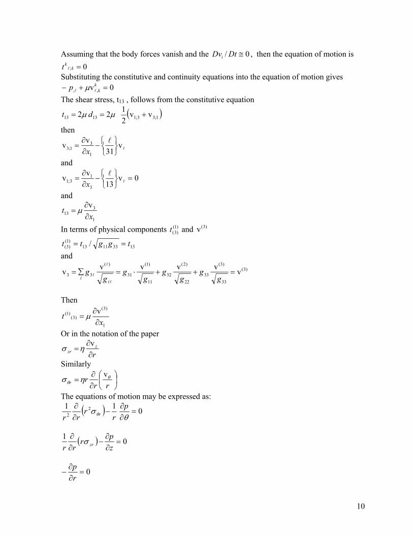
Assuming that the body forces vanish and the 0/ ≅DtDvi , then the equation of motion is 0; =k
kt l Substituting the constitutive and continuity equations into the equation of motion gives
0v ,, =+− kkp ll µ
The shear stress, t13 , follows from the constitutive equation
( )1;33;11313 vv2122 +== µµ dt
then
l
l v31
vv1
31;3
⎭⎬⎫
⎩⎨⎧−
∂∂
=x
and
0v13
vv3
13;1 =
⎭⎬⎫
⎩⎨⎧−
∂∂
= l
l
x
and
1
313
vx
t∂∂
= µ
In terms of physical components and )1()3(t
)3(v
13331113)1()3( / tggtt ==
and )3(
33
)3(
3322
)2(
3211
)1(
31
)(
33 vvvvvv =++⋅=∑=g
gg
gg
gg
gll
l
ll
Then
1
)3(
)3()1( v
xt
∂∂
= µ
Or in the notation of the paper
rz
zr ∂∂
=vησ
Similarly
⎟⎠⎞
⎜⎝⎛
∂∂
=rr
rrθ
θ ησv
The equations of motion may be expressed as:
( ) 011 22 =
∂∂
−∂∂
θσθ
pr
rrr r
( ) 01=
∂∂
−∂∂
zpr
rr zrσ
0=∂∂
−rp
10
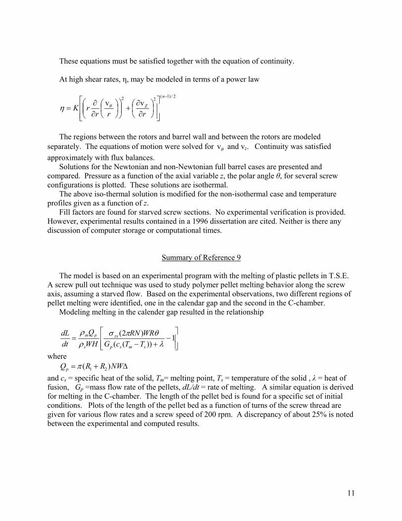
These equations must be satisfied together with the equation of continuity. At high shear rates, η, may be modeled in terms of a power law
2/)1(22vv
−
⎥⎥⎦
⎤
⎢⎢⎣
⎡⎟⎠⎞
⎜⎝⎛∂∂
+⎟⎟⎠
⎞⎜⎜⎝
⎛⎟⎠⎞
⎜⎝⎛
∂∂
=
n
Z
rrrrK θη
The regions between the rotors and barrel wall and between the rotors are modeled
separately. The equations of motion were solved for and vθv z. Continuity was satisfied approximately with flux balances.
Solutions for the Newtonian and non-Newtonian full barrel cases are presented and compared. Pressure as a function of the axial variable z, the polar angle θ, for several screw configurations is plotted. These solutions are isothermal.
The above iso-thermal solution is modified for the non-isothermal case and temperature profiles given as a function of z.
Fill factors are found for starved screw sections. No experimental verification is provided. However, experimental results contained in a 1996 dissertation are cited. Neither is there any discussion of computer storage or computational times.
Summary of Reference 9 The model is based on an experimental program with the melting of plastic pellets in T.S.E.
A screw pull out technique was used to study polymer pellet melting behavior along the screw axis, assuming a starved flow. Based on the experimental observations, two different regions of pellet melting were identified, one in the calendar gap and the second in the C-chamber.
Modeling melting in the calender gap resulted in the relationship
⎥⎥⎦
⎤
⎢⎢⎣
⎡−
+−= 1
))(()2(
λθπσ
ρρ
smsp
zx
s
pm
TTcGWRRN
WHQ
dtdL
where ∆+= NWRRQp )( 21π
and cs = specific heat of the solid, Tm= melting point, Ts = temperature of the solid , λ = heat of fusion, Gp =mass flow rate of the pellets, dL/dt = rate of melting. A similar equation is derived for melting in the C-chamber. The length of the pellet bed is found for a specific set of initial conditions. Plots of the length of the pellet bed as a function of turns of the screw thread are given for various flow rates and a screw speed of 200 rpm. A discrepancy of about 25% is noted between the experimental and computed results.
11
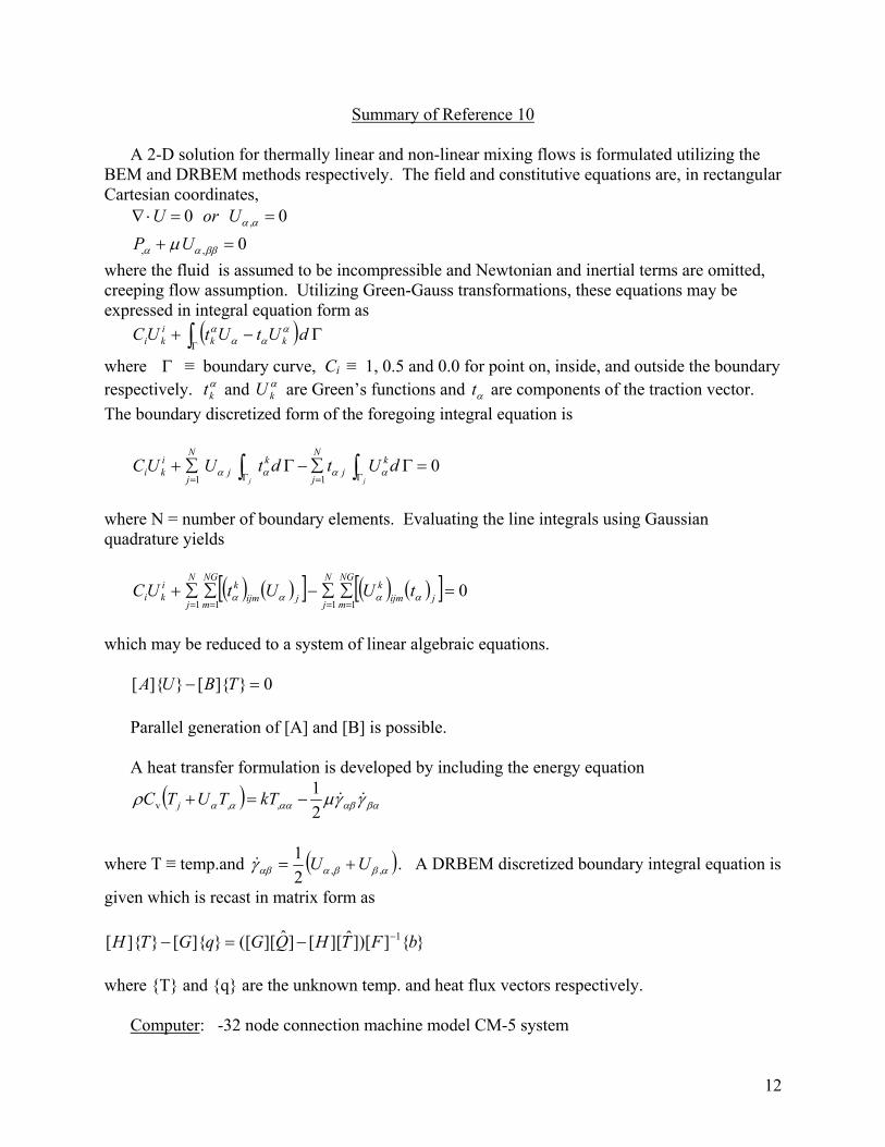
Summary of Reference 10 A 2-D solution for thermally linear and non-linear mixing flows is formulated utilizing the
BEM and DRBEM methods respectively. The field and constitutive equations are, in rectangular Cartesian coordinates,
00 , ==⋅∇ ααUorU 0,, =+ ββαα µUP
where the fluid is assumed to be incompressible and Newtonian and inertial terms are omitted, creeping flow assumption. Utilizing Green-Gauss transformations, these equations may be expressed in integral equation form as
( )∫Γ Γ−+ dUtUtUC kkiki
ααα
α
where ≡ boundary curve, CΓ i ≡ 1, 0.5 and 0.0 for point on, inside, and outside the boundary respectively. and are Green’s functions and are components of the traction vector. The boundary discretized form of the foregoing integral equation is
αkt
αkU αt
∫∫ Γ=Γ==Γ∑−Γ∑+
jj
dUtdtUUC kj
N
j
kj
N
j
iki 0
11αααα
where N = number of boundary elements. Evaluating the line integrals using Gaussian quadrature yields
( ) ( )[ ] ( ) ( )[ ] 01111
=∑∑−∑∑+====
jijmk
NG
m
N
jjijmk
NG
m
N
j
iki tUUtUC αααα
which may be reduced to a system of linear algebraic equations.
0][][ =− TBUA
Parallel generation of [A] and [B] is possible.
A heat transfer formulation is developed by including the energy equation
( ) βααβαααα γγµρ &&21
,,v −=+ kTTUTC j
where T ≡ temp.and ( αββααβγ ,,21 UU +=& ). A DRBEM discretized boundary integral equation is
given which is recast in matrix form as
]])[ˆ][[]ˆ][([][][ 1 bFTHQGqGTH −−=− where T and q are the unknown temp. and heat flux vectors respectively.
Computer: -32 node connection machine model CM-5 system
12

Program Language: CM-Fortran Mixer Geometry: -2-D, single rotor, circular barrel, rotor with a single axis of symmetry,
rotating about an axis through the center of the circular barrel and ⊥ to plane of the mixer. Boundary Conditions: - No slip on the barrel and rotor, surface temp. of the rotor and barrel
= 180°C. Material Properties: - Newtonian fluid with conductive and convective transport effects. Discretization: -379 boundary elements
209 internal solution evaluation points within the fluid Results for BEM Flow (Linear). Total running times
a. Serial ≅ 15 min. b. Parallel ≅ 1.5 min.
Results for DRBEM Flow (Non-linear). Total running times. a. Serial ≅ 110 min. b. Parallel ≅ 8.3 min.
Summary of Reference 11
The dual reciprocity boundary element method (DRBEM) is discussed and applied to the 2-D mixing of non-linear polymer rheological fluids.
Constitutive model for sheer stress:
( ) αβαβ γγητ && T,=
where )(2/1 ,, αββααβγ UU +=& . In a more familiar notation
llllm
mkkkk dddpt 21 ααδ ++−=
for a non-linear incompressible fluid where .2,1),,( == iIIIII ddii αα Omitting product terms gives
lllkkk dpt 1αδ +−=
where )vv(2/1 ;; kkkd lll +=
and
n
nk
k kx
vvv ; ⎭⎬⎫
⎩⎨⎧−
∂∂
= ll
l
Normal stress effects are discussed. It is observed that Newtonian and generalized
Newtonian fluids do not exhibit normal stress effects. Memory Effects: The Deborah number, De, flowtDe /λ=
where λ = relaxation time of the fluid, λ ≥ 0, a constitutive quantity, and tflow = characteristic time of the flow field.
13

⇒→ 0De memory effects are negligible ⇒∞→De memory effects are negligible solid like behavior
⇒≅ 1De memory effects are observed Extrudate Swell: Polymer exits the die and expands to several times the diameter of the die. Attributed to normal stresses and memory.
Field Equations, Equation of Motion, Continuity, Energy Balance
0, =ααU
( ) SUUTPTqTUTC t ++⎥⎦⎤
⎢⎣⎡∂∂
−−=+ βααβαααααα τρ ,,,v ,,
( )βαβααβαβ ρρσ ,,, UUUg t ++−= Note the retention of the acceleration terms in the equation of motion.
** The 3-D, BEM modeling of flow within a S.S.E. was accomplished by Biswas et al. in 1994, Antec, 636. DRBEM Formulation
Let ( )βαβααααβαβ ρρσ ,,, , UUUgbb t ++−==
Then the integral equations
Ω=Γ−Γ+ ∫∫∫ ΩΓΓdUbdUtdUtUC kkk
αααααααl
l
Let be a particular solutionk
βασ of . αβαβσ bk =,ˆ
Let
αα β ⎟
⎠⎞
⎜⎝⎛ ∑=
+
=jj
LN
jfb
)(2
1
and
αβαβσ )()ˆ( , jjk f=
Then
( ) ( ) Ω∑=Γ−+ ∫∫ ΩΓ dUdUtUtUC kjj
kkk αραβαααα σβ )ˆ( ,l
l The dual reciprocity method transforms the above into
14

( ) ( ) ( ) ( )( )( )Γ−+∑=Γ− ∫∫ Γ
+
=Γ dUtUtUCdUtUtUC k
jk
jkk
jk
j
LN
j
kkαααααααααα β ˆˆˆ
)(2
1l
ll
Introducing boundary conditions yields: ]])[ˆ][[]ˆ][([][][ 1 bFtGUHtGUH −−=−
A solution for counter rotation of concentric circular cylinders with a gravitational body
force is provided. Memory requirements and execution times are not given. One assumes that the acceleration terms in the equation of motion, linear and non-linear,
were not included in the solution.
Summary of Reference 12 The 2-D BEM is used to analyze and compare the mixing effectiveness of T.S.E. of various
geometries. Geometry: The 2-D fluid motion in a plan perpendicular to the axes of a 3-D T.S.E. was
modeled. The exterior boundary corresponded to the barrel of the T.S.E. Two symmetric elliptic impellers, 90° out of phase, rotate about the screw axes of the T.S.E.
Single, double, and triple flighted screws were studied. The effect of varying centerline distances between screws on mixing effectiveness was studied (random distribution of traces). The travel or deformation of a tracer line full barrel assumption, strain rate, and volumetric strain rate were computed.
Computer: DEC 5000/200 Execution Time: 7.5 min. for each time step. Time Step = 2° rotational step Fluid properties = Newtonian fluid, incompressible, creeping flow, iso-thermal.
Summary of Reference 13
This is a slight modification of Reference 12 with a more extensive set of references.
Summary of Reference 14
Reference [14] contains a 2-D, B.E. simulation of the flow of a multiple phase, multi-viscous polymer in an internal single rotor batch mixer. A creeping flow is assumed.
The field equations are:
0, =ααU and
0, , =+− ββαα µUp where α, β = 1, 2, Uα = velocity in the xα coordinate direction, p = pressure and µ = viscosity,
which is assumed to be constant for a given fluid.
15

Boundary conditions: a. Free boundary :- The traction vector tα is given, Γ1. b. Solid boundary:- No slip condition, Uα is given Γ2. c. Interfacial boundary between regions 1 & 2, Γ3.
21αα tt −= on 3Γ
21αα UU = on 3Γ
Superscripts refer to regions 1 or 2.
Integral Equation Formulation
∫Γ =Γ−= 0][ dUtUtUC kkiki αααα
Ci = 1, 0.5, 0 inside, on, or outside, respectively, of the specific domain. Here
[ ]kkk rrnrU ,,4
1ααα δ
πµ−
−= l
and
πνσ ναβαβα /,,, 1−−== rrrrt kkk
Discretized Form
( ) ( )∫∫ Γ∑−Γ∑+ Γ=
Γ=
dUtdUtUC k
NP
jk
NP
j
iki jj
ααα
α
11
where NP = number of boundary elements. Constant boundary elements were assumed where the values of Uα and tα are assumed to be constant on each element and equal to their values at the midpoint. The discretized form is then
011
=Γ∑−Γ∑+ ∫∫ Γ=
Γ=
dUtdtUUC kj
NP
jkj
NP
j
iki jj
αα
αα
Evaluating the integrals, utilizing Gaussian quadrature, and placing point i on each element center yields a matrix equation
[A] X = R where X is a vector of unknowns Uα and tα. [A] is composed of submatrices associated
with each domain, [Ai]. These appear on the diagonal of [A] and are linked by a matrix [C]. In general [Ai] is composed of coefficients of the unknown parameters of the i-th domain. It appears that the new position of a domain is estimated from the previous position through a
calculation. tU ∆⋅α
The deformation of a small circular drop of viscosity µ 2 surrounded by a fluid of viscosity µ1 in a 2-D single rotor mixer is presented. A three domain simulation of flow between parallel plates is also given.
No information regarding computer execution times or memory size requirements is given.
16

Summary of Reference 15 Reference [15] presents a 3-D computer simulation of the flow in a S.S.E. with a rhomboidal
mixing section. Mixer geometry: 3-D, single screw extruder, circular barrel, screw diameter, 6.55-21.82mm,
pitch, 1D-4D, number of cuts, 4-6. A number of mixing sections were considered. The barrel diameter and mixing section length are not given.
Material properties: Newtonian fluid, constant viscosity, incompressible, creeping flow. Boundary conditions: No slip on all surfaces. No free surfaces. Full barrel flow. Computational algorithm: 3-D, BEM, quadratic shell elements. Computational requirements: 1000-1400 quadratic shell elements, 4200 nodes, 200 tracer
particles, execution time on a Silicon Graphics Indigo 2 R1000 was 4 hours to solve for unknowns. I assume that this timing was for a converged solution and not a single step. Tracer tracking execution time was 20 hours. ≅
Computer specifications: The Silicon Graphics Indigo 2 R1000 operates at 195 MHz. Desktop systems operating at 3.6 GHz are currently available, giving a ratio of 18:1. Allowing for improvements in memory access and internal information transfer would probably increase this ratio to 20:1. Then execution time would be
≅
≅ 12 min. and 60 min. respectively. Distributive mixing: Homogenization of a secondary phase within the fluid matrix and is
dependent on the amount of strain imposed on the material. Total strain measure is
∫=1
0
1 )()(t
dttt γγ &&
where )(tγ& is the magnitude of the strain rate. Flow number: The flow number = λ is defined as )/( w+= γγλ &&
wandγ&where are the magnitude of the strain rate (does the author mean deformation rate?)
and vorticity tensors, respectively. The vorticity tensor, )vv(21
,, kllkklw −= which can be
expressed as an axial vector such that . Then the magnitude of the vorticity tensor could be defined as the magnitude of the vorticity vector. The stretching in the direction of a unit vector,
kw lmklmk ew ,v=
n is defined as
lkkln nnddsDTD
dsd == )(1
)(
The magnitude of may be what is defined by )(nd γ& . a. Pure rotational flow, λ = 0.0 b. Pure elongational flow, λ =1.0 c. Shear flow, λ = 0.5 Dispersive mixing: Breaking of the secondary flow into smaller particles. High stresses are
required, which is dependent on the rate of strain. Pressure and Torque Analysis Torque defines the size of the motor and screw of the extruder and is important in calculating
the efficiency of the mixer. In general, the lower the torque and required pressure for a given flow rate the more efficient the extruder will be.
17
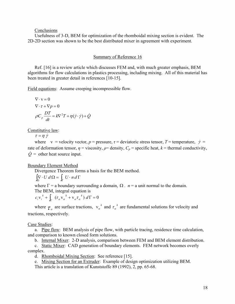
Conclusions Usefulness of 3-D, BEM for optimization of the rhomboidal mixing section is evident. The
2D-2D section was shown to be the best distributed mixer in agreement with experiment.
Summary of Reference 16
Ref. [16] is a review article which discusses FEM and, with much greater emphasis, BEM
algorithms for flow calculations in plastics processing, including mixing. All of this material has been treated in greater detail in references [10-15].
Field equations: Assume creeping incompressible flow.
QTkdt
DTC
p
p&&& +⋅+∇=
=∇+⋅∇=⋅∇
)(
00v
2 γγηρ
τ
Constitutive law:
γητ &= where v = velocity vector, p = pressure, τ = deviatoric stress tensor, T = temperature, γ& =
rate of deformation tensor, η = viscosity, ρ= density, Cp = specific heat, k = thermal conductivity, = other heat source input. Q&
Boundary Element Method
Divergence Theorem forms a basis for the BEM method.
∫∫ ΓΩΓ⋅=Ω⋅∇ dnUdU
where Γ = a boundary surrounding a domain, Ω . n = a unit normal to the domain. The BEM, integral equation is
0)vv(v =Γ++ ∫Γ dc kkkii αααα ττ
where τα are surface tractions, and are fundamental solutions for velocity and
tractions, respectively.
kαv k
ατ
Case Studies:
a. Pipe flow: BEM analysis of pipe flow, with particle tracing, residence time calculation, and comparison to known closed form solutions.
b. Internal Mixer: 2-D analysis, comparison between FEM and BEM element distribution. c. Static Mixer: CAD generation of boundary elements. FEM network becomes overly
complex. d. Rhomboidal Mixing Section: See reference [15]. e. Mixing Section for an Extruder: Example of design optimization utilizing BEM. This article is a translation of Kunststoffe 89 (1992), 2, pp. 65-68.
18

Review of Reference 17 This comprehensive review article is a translation of “Verarbeitun gsprozesse mit Modellen
beschreiben”, Kunststoffe 10/2003, pp. 130-134, which contains all of the figures. References must be obtained directly from the author online.
Included is a discussion of FEM with much greater emphasis on BEM algorithms for flow calculations in plastics processing, including mixing. All of the material on BEM in mixing has been treated in much greater detail in references [10-15].
Describing Geometrics with Models
A brief history of modeling and simulation in plastics processing beginning in the 1950s with the work of Bird, Stewart, and Lightfoot. Flow models based on simplification of the basic field equations and or geometry are compared to models based on FDM, FEM or BEM analysis. The fundamental physical laws required in processing methods in plastics technology are mentioned. Process Simulation
Plays a role in the design of moulds for injection moulding, compression moulding, and extrusion dies. A brief discussion of the Hele-Shaw model is included. The Finite Difference Method, FDM
History of FDM applications in injection moulding, compression moulding, and one-dimensional approximation. The Hele-Shaw model and FAN analysis are discussed. 3-D, FAN has been applied to flows in TSE. Applications of the finite volume flow method are discussed. See references [8, 9]. Finite Element Analysis
A history of applications of FEM in plastics technology with a paragraph on 2 and 3-D simulations of mixing processes. See references [1-7]. The Boundary Element Method
A review of the theory and application of BEM to TSE. See references [10-18].
Review of Reference 18 This is another review article, each section of which will be summarized in turn. 1. Introduction: The author gives general observations regarding 3-D simulations. He
focuses on problems associated with moving boundaries, making the distinction between moving, free and solid boundaries. A hierarchy of computational complexity in the numerical modeling of single and twin screw extruders is presented.
“The complete simulation of the T.S.E. process including melting, melt conveying, mixing,
die flow, and partially filled systems should be regarded as one of the grand challenge problems in polymer processing.”
19

2. Rheology: Caution: The author appears to conflate shear strain rate and deformation rate. The deformation rate tensor is defined as:
)vv(21
,, ijjiijd +=
The material derivative of the Lagrangian strain tensor is:
LlKklkKL xxdEDtD
,,)( =
The material derivative of the Eulerian strain tensor is:
mLkKKLlmlLmKKLkmklkl XXEXXEdeDtD
,,,,,, vv)( −−=
For infinitesimal deformations:
lLkKklKL dEDtD δδ≅)(
The constitutive equations for incompressible fluids are of the form:
),,( θθδ ∇+−= ijklklkl dfpt ),,( θθ∇= ijkk dgq
θθθ∂Ψ∂
−Ψ∈= )(
θη ∂Ψ−∂= /
0,2
2
=+++∂Ψ∂ hqdf kkklklo ρθθ
θρ &
where θ = temp., f and g satisfy various inequalities, ∈= internal energy density, η = entropy, etc.
It is clear that the constitutive equations of a general incompressible fluid is expressed in terms of dkl , the rate of deformation tensor rather than any of the several strain rates.
The author considers generalized Newtonian fluids, GNF, which is linear in the stress tensor and of the form
klklkl dpt µδ 2+−=
where ),( ijdθµµ = . Again, tkl is given as a function of dkl.
Models are discussed in which µ is modeled in various ways included in the following: a. Carreau’s model – See the Summary of Reference [1] b. Cross’s model – See the Summary of Reference [2] c. Bingham fluid – See the Summary of Reference [6] d. Herschel-Bulkley model – See the Summary of Reference [7] e. Power Law – See the Summary of Reference [8]
20
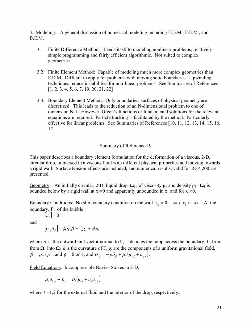
3. Modeling: A general discussion of numerical modeling including F.D.M., F.E.M., and B.E.M.
3.1 Finite Difference Method: Lends itself to modeling nonlinear problems, relatively simple programming and fairly efficient algorithmic. Not suited to complex geometries.
3.2 Finite Element Method: Capable of modeling much more complex geometries than
F.D.M. Difficult to apply for problems with moving solid boundaries. Upwinding techniques reduce instabilities for non-linear problems. See Summaries of References [1, 2, 3, 4, 5, 6, 7, 19, 20, 21, 22]
3.3. Boundary Element Method: Only boundaries, surfaces of physical geometry are
discretized. This leads to the reduction of an N-dimensional problem to one of dimension N-1. However, Green’s functions or fundamental solutions for the relevant equations are required. Particle tracking is facilitated by the method. Particularly effective for linear problems. See Summaries of References [10, 11, 12, 13, 14, 15, 16, 17].
Summary of Reference 19 This paper describes a boundary element formulation for the deformation of a viscous, 2-D, circular drop, immersed in a viscous fluid with different physical properties and moving towards a rigid wall. Surface tension effects are included, and numerical results, valid for Re ≤ 200 are presented. Geometry: An initially circular, 2-D, liquid drop Ω1 , of viscosity µ1 and density ρ1. Ω1 is bounded below by a rigid wall at x2=0 and apparently unbounded in x1 and for x2>0. Boundary Conditions: No slip boundary condition on the wall +∞<<∞−= 12 ,0 xx . At the boundary, Γ, of the bubble [ ] 0=iuand [ ] ( ) iijij kng γβφρησ +−= 11 where η is the outward unit vector normal to Γ, [] denotes the jump across the boundary, Γ, from from Ω1 into Ω2, k is the curvature of Γ, gi are the components of a uniform gravitational field,
12 / ρρβ = , and 1or0=φ , and ( )ijjiijij uup ,, ++−= lµδσ . Field Equations: Incompressible Navier-Stokes in 2-D, ( )jijtiijji uuupu ,,,, +=− ll ρµ where =1,2 for the external fluid and the interior of the drop, respectively. l
21

Continuity for an incompressible fluid, 0, =iiu There are three coupled, non-linear partial differential equations in u1, u2, and p. Constitutive Equations: ( )ijjiijij uup ,, ++−= lµδσ where µ = constant. B.E.M. Formulation
The integral representation formula for the exterior velocity is
Ω+
Γ−
=Γ−
∫∫∫
Ω
Γ
Γ
dxdxxu
dxnxuxxu
dxuxxkxu
ij
ji
kjkj
i
jiji
)(),(/1
)()))(()(,(/1
))()(,()(
01
101
100
1µ
σµ
An equation of similar form applies to the interior of the fluid drop, where
)( ,, jijtii uud += µρl
l
Note that is an integral over a 2-D domain which is approximated by a boundary
integral, , through the dual reciprocity approximation. ΩΩ∫ d)(
1
Γ∫Γ d)(
Assuming that 21 and ρρ are constant and transforming the domain integrals in the previous
integral representations yields in matrix notation,
α⎥⎦⎤
⎢⎣⎡ −−=+− GTHUaUaGtaHuau 3421 21
21
where u and t are the velocities and tractions, α is an unknown, H, G, U, and T are matrices of known functions. A first order explicit time integration is employed in which
( ) dtuutu m
imi
i /1 −≅∂∂ +
22

Numerical Examples
Numerical results are provided for several examples, including: a. Recovery of circular drop shape, due to surface tension, from an elliptical shape with no
initial velocity or gravitational field. b. Motion of a drop towards a rigid wall, in a gravitational field, starting from a circular
shape with zero velocity. Computational Requirements:
A parallel processor with two 2.0 GHz Pentium III processors and 1.0 GB of RAM were employed. The drop boundary, Γ, was discretized by 40 nodes. Integrations employed 20 Gaussian integration points. Typical computational times were of the order of 1.0 min. for 100 time steps.
Summary of Reference 20
The authors have applied 3-D F.E.M. modeling to the study of the effects of screw speed, entering peroxide distribution and pressure to drag flow ratio on the mixing of steady, incompressible, non-isothermal reactive flows in a forward conveying element of a T.S.E. Mixer Geometry: The 3-D flow in a single fully filled conveying element channel of a TSE is modeled. Screw o.d. = 33.7mm, no. of screw flights = 2, screw centerline separation, channel depth = 3.7mm, pitch = 20mm, channel aspect ratio = 2.8. Field Equations:
Conservation of mass assuming incompressibility: 0v =⋅∇
Momentum equation for steady flow: vv)(ρτ ⋅−∇=∇+⋅∇ P Energy assuming that thermodynamic properties are constant.
)v(v2 TcTk p ∇⋅=∇⋅−∇ ρτ
Material Properties Constitutive Equation:
γητ &−= where
00
00
,)),(1(),()(,)),(1(),()(
γγγηγγγη&&&lll
&&&lll
>−−=<−−=
nMTnMTKnnnMTnMTKnn
where 0γ& = 10s-1, T = temp., M = average molecular weight, melt density = 750 kg/m3, melt thermal conductivity = 0.185 w/m°C, Specific heat capacity = 2.428kJ/(kg°C), entering w-a molecular weight = 330,000, n-a molecular weight = 43,420.
23

Reactive Processes Described by species mass conservation equations (no molecular diffusion) for the peroxide as well as for the three moments of the polymer MWD. Peroxide data used for 2, 5 dimethyl-2, 5-di-tert-butylperoxyhexane.
)/()2(2
)/()2(2
)/(22
)/()3((2
012
10223
0103/13/32
0101
01010
QQQQQQQ
QQQQQIfkQ
QQQIfkQ
QQQQIfkQ
IkI
D
D
D
D
−=
−−+−−=
−⋅−=
−−=
−=
&
&
&
&
The average molecular weight of the polymer is given by 120 / QQMM =The peroxide decomposition rate constant is
( )2
12
)(1364.00243.06294.0
)15.273/(14947()10981(
nMTMnKn
Tnkn D
lll
ll
+−−=
+−⋅⋅⋅=
n-1 is given as a function of T. Operating Conditions Inlet temp. = 220°C, barrel wall temp. = 240°C, screw speed = 100, 250rpm, pressure to drage flow ratio = 0, -0.25, average inlet peroxide level = 0, 0.6% wt. Boundary Conditions: No slip condition on the barrel and screw surfaces. For the peroxide weight fraction, zero flux b.c. were used for the screw and barrel surfaces. Computer Simulation:
A mixed discontinuous pressure formulation was used in which one pressure DOF was solved for per brick element. A fixed streamline upwinding factor was used for temp. with an element based dynamic relaxation scheme for all DOFs. For the reactive extrusion simulations, an additional dynamic viscosity relaxation scheme was used to stabilize the solution over the first 20 iterations.
Number of nodes = 12625 and 15121 and number of elements = 10560 and 12740 for 100 and 250 rpm. respectively.
Axial length = 61.2mm. Cross-sectional area in the translation region = 22.0mm2.
Computer Requirements FIDAP version 7.62 was run on an IBM Risc/6000 workstation with 128MB RAM.
Execution times were not provided.
24

Results Sixteen cases were considered for which average temp. profiles, pressure profiles, peroxide
conversion profiles, flow efficiencies, and average molecular weight profiles were computed. No comparisons with experimental data were provided.
Summary of Reference 21 The authors model a partially filled, 2-D, internal mixer utilizing intermeshing blades with
very long tips. The transient, non-isothermal, generalized Newtonian flow and mixing of a polymer-filler compound is studied in a free surface regime consisting of incompressible and compressible parts.
Mixer Geometry:
2-D, internal mixer with 2 rotating long blades and partially filled.
Field Equations: Continuity Equation: a. Incompressible phase - 2,1,0v , == iii
b. Compressible phase - 0)v( ,, =+ iit ρρ c. Equation of motion - )vvv( ,,,, jijtiijij p +=− ρτ d. Energy equation - 2
,,, )()v( γηρ &+=+ jjjjt TKTTce. Carbon black concentration equation - 0v ,, =+ iit CC where C = concentration of carbon black.
Material Properties:
)())(1()2/)1(()()(
)vv(21,2
20
,,
r
ijjiijijij
TTbnnnn
dd
−−+−−=
+==
γληη
ητ
&lll
The strain rate γλ & is given by
ijij dd2)( 2 =γλ & The relative viscosity, rη , of the rubber-carbon compound at different times is given by
Φ+= 5.51rη where Φ = effective volume fraction of carbon black.
25

1
,,
021.0where][],[
].,[v
−=−Φ≅Φ
Φ=Φ+Φ=Φ
sKCKCS
CSDtD
iit
Boundary Conditions:
Free surface equation – Tracking of the free surface is carried out via the solution of the probability distribution
density distribution equation for the free surface function, F, 0v ,, =+ iit FF
In sections filled with rubber, F = 1, in air-filled regions or a vacuum F = 0. F = 0.5 indicates a free surface boundary between rubber and air filled or vacuum regions.
The no-slip condition applies to all solid boundaries.
Solution Algorithm: The Galerkin F.E.M. together with the upwind Petrov Galerkin method is utilized. Since the
resulting equations are non-linear, an iteration method is employed in which flow, energy, free surface and mixing dependent viscosity equations are solved successively at each iteration cycle.
Computer Requirements and Execution Times:
These are not given.
Results: Solutions are given for an initial configuration of two rotating blades in an 81% full chamber.
Predicted free surface distributions are given for rotations of 30°, 60°, 90°, 180°, together with contours of high temp. regions.
Summary of Reference 22 Reference [22] presents an F.E.M. analysis of a fully filled, 2-D, internal, single bladed
mixer. A nonlinear, incompressible, viscoelastic fluid model was used with parameters appropriate for a dough-like material. Elastic-viscous stress splitting, stress sub-elements and upwind Petrov-Galerkin were employed to compute viscoelastic limits.
Mixer Geometry:
Fully filled, 2-D, cylindrical, internal single bladed mixer.
Field Equations: a. Conservation of mass – (incompressible) 2,1,0v , == iii
b. Equation of motion – (matrix notation)
0]v[)2( 21 =−+−+⋅∇ fdtdpIDT ρη
where I = identity matrix, T1 = matrix of non-viscous stress components, p = pressure, D = matrix of rate of deformation components.
26

c. Energy Equation – Not used in the calculation. Temp. effects are neglected.
Material Properties:
a. Constitutive equations –
)~2
)2
1(()/)(exp(2 111111 TTTTtrD ξξληελη +−+=
b. Stress splitting – T=T1+T2 where DT 22 2η= is the viscous component, T is the total stress tensor and T1 is the residual
component. c. Viscosity ratio – 9/1)/( 211 =+ηηη
d. 211 )
21(~
2TT
dtdT ξξ
−+=
e. Bird-Carreau viscous model – 2/)1(22
4041 )1)(( −+−+= nγληηηη
Boundary Conditions: No slip boundary conditions on all surfaces.
Solution Algorithm: A mixed Galerkin formulation of the governing equations was used. Finite expansions of T1,
v, and p were made in terms of the F. E. basis functions. The field equations were recast in integral form involving the basis functions. 4x4 subelements for the stress were used together with the elastic-viscous stress splitting. Stability problems were resolved by gradually introducing the source of the instability into the computation. This was done by reducing the mixing speed or the relaxation time.
Results:
Pressure vs. the spatial coordinate was given for a range of relaxation times for mixing
speeds of 1 and 100 r.p.m.. A comparison was made with results from the Bird-Carreau viscous model. Velocity fields were plotted for various relaxation times and mixing speeds.
Computer Requirements and Execution Time
Meshes of from 360 to 3360 elements were tested. A 2080 element mesh proved to be
optimal. Memory requirements and execution times were not provided.
27
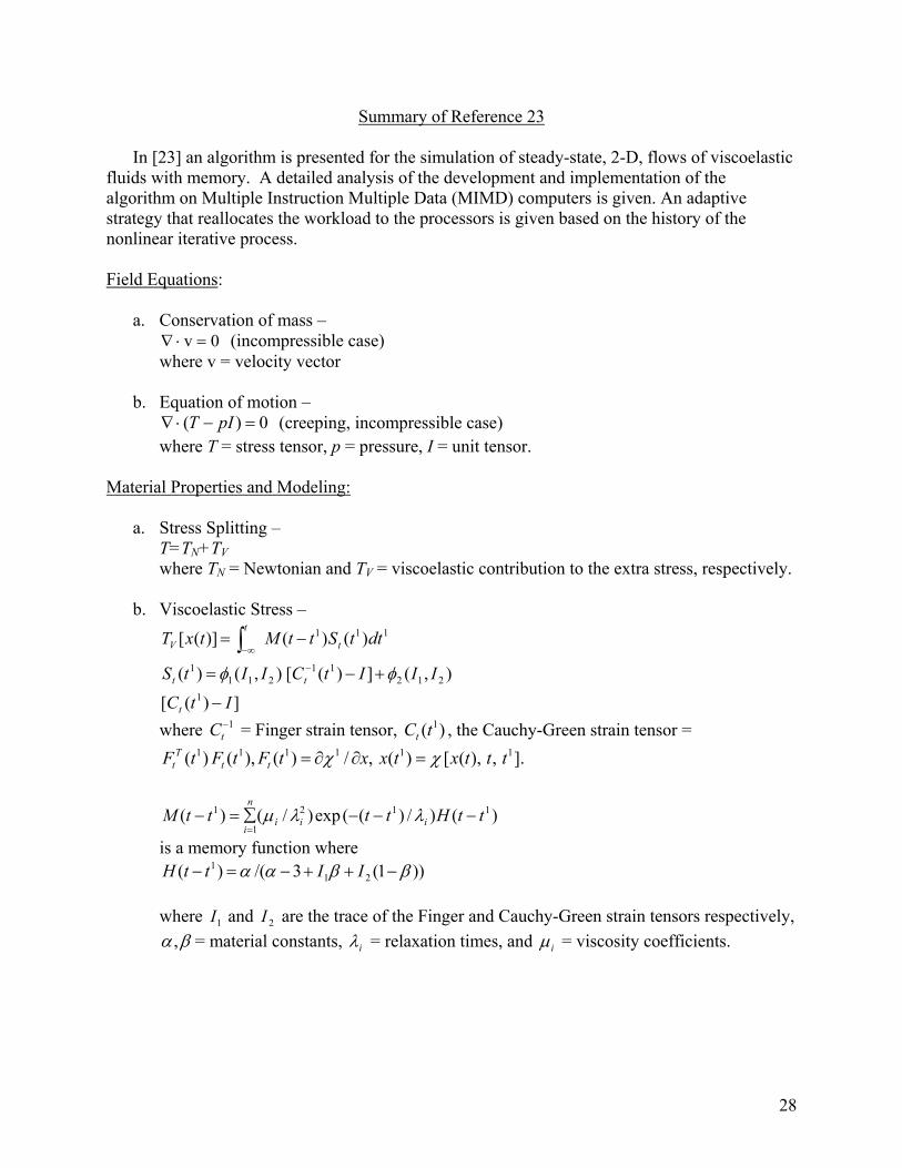
Summary of Reference 23 In [23] an algorithm is presented for the simulation of steady-state, 2-D, flows of viscoelastic
fluids with memory. A detailed analysis of the development and implementation of the algorithm on Multiple Instruction Multiple Data (MIMD) computers is given. An adaptive strategy that reallocates the workload to the processors is given based on the history of the nonlinear iterative process.
Field Equations:
a. Conservation of mass – (incompressible case) 0v =⋅∇ where v = velocity vector b. Equation of motion – (creeping, incompressible case) 0)( =−⋅∇ pIT where T = stress tensor, p = pressure, I = unit tensor.
Material Properties and Modeling: a. Stress Splitting – T=TN+TV where TN = Newtonian and TV = viscoelastic contribution to the extra stress, respectively. b. Viscoelastic Stress – 111 )()()]([ dttSttMtxT t
t
V −= ∫ ∞−
])([
),(])([),()(1
21211
2111
ItC
IIItCIItS
t
tt
−
+−= − φφ
where = Finger strain tensor, , the Cauchy-Green strain tensor = 1−tC )( 1tCt
].,),([)(,/)(),()( 111111 tttxtxxtFtFtF ttT
t χχ =∂∂=
)()/)((exp)/()( 112
1
1 ttHttttM iii
n
i−−−∑=−
=λλµ
is a memory function where ))1(3/()( 21
1 ββαα −++−=− IIttH
where and are the trace of the Finger and Cauchy-Green strain tensors respectively, 1I 2Iβα , = material constants, iλ = relaxation times, and iµ = viscosity coefficients.
28

Results: The numerical solution of the 2-D flow for the memory-dependent viscoelastic fluid through
an abrupt construction is presented with a detailed discussion of the computer implementation. The finite element mesh has 256 elements.
Computer Implementation:
The parallel algorithm was implemented within POLYFLOW using the communication
library of the Intel iPSC/860 hypercube. It has been found relatively easy to transfer the Intel hypercube code to other MIMD computers such as the Convex Meta Series.
The solution of the pseudo-Stokes problem with the viscoelastic extra stresses taken as body forces is solved with the mixed velocity-pressure formulation and the standard Galerkin F.E.M.. A nonlinear iteration is started from a Newtonian flow field. The viscoelastic solution follows from the solution of the Newtonian flow through an incremental loading procedure.
The finite element mesh has 256 elements. No-slip boundary conditions at the wall, symmetry boundary conditions along the axis of symmetry, and fully developed Poiseville flow at the inlet and outlet sections were conditions imposed on the flow.
29

REFERENCES [1] T. Ishikawa et al., Numerical Simulation and Experimental Verification of Nonisothermal
Flow in Counter-Rotating Nonintermeshing Continuous Mixers, Polymer Engineering and Science, Feb. 2000, Vol. 40, No. 2.
[2] T. Ishikawa, S. I. Kihara, and K. Funatsu, 3-D Numerical Simulations of Nonisothermal
Flow in Co-Rotating Twin Screw Extruders, Polymer Engineering and Science, Feb. 2000, Vol. 40, No. 2.
[3] T. Ishikawa and T. Amano, Flow Patterns and Mixing Mechanisms in the Screw Mixing
Element of a Co-Rotating Twin Screw Extruder, Polymer Engineering and Science, May 2002, Vol. 42, No. 5.
[4] M. Yoshinaga, Mixing Mechanism of Three-Tip Kneading Block in Twin Screw
Extruders, Polymer Engineering and Science, January 2000, Vol. 40, No. 1. [5] A. Lawal and D. M. Kalyon, Mechanisms of Mixing in Single and Co-Rotating Twin
Screw Extruders, Polymer Engineering and Science, 1995, Vol. 35, No. 17, 1325-1337. [6] A. Lawal, S. Railkar, et al., 3-D Analysis of Fully Flighted Screws of Co-Rotating Twin
Screw Extruder, SPE ANTEC, 1996, 42, 155-159. [7] D. M. Kalyon, A. Lawal, et al., Mathematical Modeling and Experimental Studies of
T.S.E. of Filled Polymers, Polymer Engineering and Science, 1999, Vol. 39, No. 6, 1139-1151.
[8] M. H. Hong and J. L. White, Simulation of Flow in an Intermeshing Modular Counter-
Rotating Twin Screw Extruder: Non-Newtonian and Non-Isothermal Behavior, International Polymer Processing XIV, 1999, 2, 136-143.
[9] K. Wilczynski and J. L. White, Melting Model for Intermeshing Counter-Rotating Twin
Screw Extruders, Polymer Engineering and Science, 2003, Vol. 43, No. 10, 1715-1726. [10] B. A. Davis and T. A. Osswald, Modeling and Simulation in Polymer Processing Using
Parallel Computing, Parallel Computing in Multiphase Flow Systems Simulations, S. Kim, G. Karniadakis, M. K. Vernon, eds., FED-Vol. 199, ASME, 1994, 61-67.
[11] B. A. Davis and T. A. Osswald, A Non-Newtonian Simulation Method for Moving
Boundary Problems, ANTEC 95, 1146-1150. [12] P. J. Gramann, A. C. Rios, and T. A. Osswald, Comparative Study of Mixing in Twin
Screw Extruders, ANTEC 95, 108-112.
30

[13] A. C. Rios, P. J. Gramann, and T. A. Osswald, Comparative Study of Mixing in Corotating Twin Screw Extruders Using Computer Simulation, Advances in Polymer Technology, 1998, Vol. 17, No. 2, 107-113.
[14] L. Stradins and T. A. Osswald, Simulating the Flow of Multi-Domain Polymer Blends
During Mixing Using BEM, Engineering Analysis with Boundary Elements, 1995, Vol. 16, 197-202.
[15] A. C. Rios, P. J. Gramann, et al., Comparative Study of Rhomboidal Distributive Mixing
Sections Using Computer Modeling, Proceedings of the Society of Plastics Engin., Conf. 56, 1998, Vol. 1.
[16] T. A. Osswald, BEM in Plastics Processing, Kunststoffe plast europe, 1999, 89, 2, 65-68. [17] T. A. Osswald, Describing Processing Operations with Models, Kunststoffe plast europe,
2003, 10, 130-134. [18] T. A. Osswald, Polymer Processing Simulations Trends, SAMPE, Erlangen, Germany,
2001. [19] J. P. Hernandez, T. A. Osswald, and D. A. Weiss, Simulation of Viscous, 2-D Planar
Cylindrical Deformation Using DR-BEM, International Journal of Numerical Methods for Heat and Fluid Flow, 2003, 13, 6, 698-719.
[20] D. Strutt, C. Tzoganakis, et al., Mixing Analysis of Reactive Polymer Flow in Conveying
Elements of a Co-Rotating Twin Screw Extruder, Advances in Polymer Technology, 2000, Vol. 19, No. 1, 22-33.
[21] V. Nassehi and M. H. R. Ghoreishy, Modeling of Mixing in Internal Mixers with Long
Blade Tips, Advances in Polymer Technology, 2001, Vol. 20, No. 2, 132-145. [22] R. K. Connelly and J. L. Kokini, 2-D Numerical Simulation of Differential Viscoelastic
Fluids in a Single-Screw Continuous Mixer: Application of Viscoelastic Finite Element Methods, Advances in Polymer Technology, 2003, Vol. 22, No. 1, 22-41.
[23] R. Aggarwal and R. Keunings, Simulation of the Flow of Integral Viscoelastic Fluids on
a Distributed Memory Parallel Computer, Journal of Rheology, 1994, Vol. 38, No. 2, 405-419.
31