a macroscopic signal optimization model for … macroscopic signal optimization model for arterials...

IEEE TRANSACTIONS ON INTELLIGENT TRANSPORTATION SYSTEMS, VOL. 15, NO. 2, APRIL 2014 805

A Macroscopic Signal Optimization Model forArterials Under Heavy Mixed Traffic Flows

Yen-Yu Chen and Gang-Len Chang, Member, IEEE

Abstract—This paper presents a generalized signal optimizationmodel for arterials experiencing multiclass traffic flows. Insteadof using conversion factors for nonpassenger cars, the proposedmodel applies a macroscopic simulation concept to capture thecomplex interactions between different types of vehicles fromlink entry and propagation, to intersection queue formation anddischarging. Since both vehicle size and link length are consideredin modeling traffic evolution, the resulting signal timings can bestprevent the queue spillback due to insufficient bay length andthe presence of a high volume of transit or other types of largevehicles. The efficiency of the proposed model has been comparedwith the benchmark program TRANSYT-7F under both passen-ger flows only and multiclass traffic scenarios from modest tosaturated traffic conditions. Using the measures of effectiveness ofthe average-delay-per-intersection approach and the total arterialthroughput during the control period, our extensive numerical re-sults have demonstrated the superior performance of the proposedmodel during congested and/or multiclass traffic conditions. Thesuccess of the proposed model offers a new signal design methodfor arterials in congested downtowns or megacities where transitvehicles constitute a major portion of traffic flows.

Index Terms—Arterial control, multiclass traffic, signaloptimization.

I. INTRODUCTION

B EST using roadway capacity to contend with daily recur-rent congestion has long been a priority task of urban

traffic professionals. Over the past several decades, both re-searchers and practitioners have devoted tremendous resourcesto tackle this vital issue with various signal control strategies,such as arterial signal progression and responsive or proac-tive signal optimization systems. The emergence of intelligenttransportation systems (ITS) since 1990s has also advanced theurban signal research to the real-time control level, based onmultisource information available from the infrastructure andnetwork vehicles. However, despite the immense potential ofusing advanced technologies to better capture traffic conditions,

Manuscript received May 27, 2013; revised August 22, 2013 and October 11,2013; accepted October 22, 2013. Date of publication November 26, 2013; dateof current version March 28, 2014. The Associate Editor for this paper wasJ. E. Naranjo.

Y.-Y. Chen is with the Department of Transportation Technology and Man-agement, National Chiao Tung University, Hsinchu 30050, Taiwan (e-mail:[email protected]).

G.-L. Chang is with the Department of Civil and Environmental Engineer-ing, University of Maryland, College Park, MD 20742 USA (e-mail: [email protected]).

Color versions of one or more of the figures in this paper are available onlineat http://ieeexplore.ieee.org.

Digital Object Identifier 10.1109/TITS.2013.2289961

most cities in both developed and developing countries stilldepend on pretimed signal strategies to control their daily trafficcongestion.

In review of the literature, it is noticeable that most existingstudies on the subject of arterial signal optimization fall into oneof the following two categories: the mathematical programmingapproach and the simulation-based method. Some pioneeringmodels on the former category focused on maximizing arte-rial progression bandwidth with a set of mixed-integer linearprogramming formulations, giving less attention to flow inter-ruptions caused by heavy or unbalanced turning volume [1]–[7]. More recent studies along the same line mainly addressedon producing signal timings to minimize the total arterial in-tersection delay [8], [9]. Despite the significant contribution ofthose models in the literature, the nature of mathematical pro-gramming formulations has limited their flexibility to capturecomplex intersection flow relations, such as the overflow fromthe tuning bay and the mutual lane blockage between throughand turning lanes.

The latter category of studies aimed at capturing the complexinteractions between traffic flows and their evolution underdifferent signal phases using a simulation-based approach.TRANSYT-7F is one of the most well-recognized models inthis category, which applies macroscopic traffic-flow formula-tions to model interrelations between arterial vehicle evolutionand intersection queue formation. A near-optimal set of signaltiming plans can be then generated via the imbedded searchalgorithms based on a predefined performance index [10], [11].This simulation-based methodology has also been extended toperform online responsive signal optimization, based on real-time detected traffic data from available sensors. Examplesof such systems include Sydney Coordinated Adaptive TrafficSystem (SCATS) [12], Split, Cycle, and Offset Optimization(SCOOT) [13], OPAC [14], and RHODES [15].

Using a similar concept but with different mathematicalformulations, traffic control researchers have also producedvarious arterial signal optimization strategies, including store-and-forward models [16]–[18], queue-dispersion models [19]–[21], stochastic models [22], and discrete-time kinematicmodels [23]–[25]. Most of such studies, however, addressedmainly the undersaturated traffic conditions, giving less atten-tion to the queue spillback and lane-blockage issues when thearterial links or turning bays become a potential congestion-contributing factor.

In parallel with the given studies for undersaturated arterials,some traffic researchers have developed various models foroversaturated intersections by distributing the delays caused

1524-9050 © 2013 IEEE. Personal use is permitted, but republication/redistribution requires IEEE permission.See http://www.ieee.org/publications_standards/publications/rights/index.html for more information.

806 IEEE TRANSACTIONS ON INTELLIGENT TRANSPORTATION SYSTEMS, VOL. 15, NO. 2, APRIL 2014

by an oversaturated link to several intersections in the samearterial. For example, some researchers [26]–[28] developed a“bang–bang” control process to identify the optimal switchingpoint for signal timings among intersections in an arterial.Their models were extended later to contend with variousoversaturated intersections using flow propagation relationships[29], [30]. Along the same line, Abu-Lebdeh and Benekohal[31] modeled the intersection queue formation and dissipationat oversaturated links with a set of dynamic discrete formula-tions, and produced the optimal signal solutions with geneticalgorithms (GA) [32] that can distribute excessive queues tomultiple intersections over multiple cycles. Abu-Lebdeh et al.[33] later also presented a model that can capture the interac-tions of traffic throughput between neighboring intersections.

To tackle the complex oversaturated traffic issues, re-searchers for TRANSYT-7F [34] introduced a penalty functionto the queue in its performance index if blockages betweenlanes occur. This enhanced version also enables users to havethe option of using multiple cycles or a stepwise simulationprogram to account for spillback affects. Recently releasedversions of TRANSYT [35] has addressed this issue with a celltransmission model that offers more realistic illustration of thetime-varying queue blocking effects between neighboring lanesand intersections. Using the same simulation-based concept butwith different macroscopic formulations for traffic evolutionand flow interactions, many researchers explored various mod-els to capture dynamic queue interactions between neighboringintersections that subsequently affect the queue discharging rateand the resulting green time needs [36]–[39].

Despite the promising progress made by those studies inthe literature on arterial signal optimization for both under-saturated and oversaturated traffic conditions, most existingmodels focused on signal control for arterials comprisingmainly of passenger-car traffic and assumed that a typicallysmall percentage of nonpassenger-car flows can be convertedto equivalent passenger-car units (PCUs) [40], [41]. This typeof conversion method even with volume-dependent factors(McTrans, 2008), however, may significantly underestimate theintersection queue and delay if traffic volume consists of alarge percentage of nonpassenger-car flows, such as buses orcommercial vehicles, as in many cities where transit vehiclesconstitute a major portion of urban commuting traffic. Theeffects of large vehicles on the delay, queue formation, linkspillback, and lane blockage would be particularly pronouncedwhen the link length between neighboring intersections isrelative short and the turning bay is likely to be insufficientdue to the right-of-way constraints, which are quite commonin many urban downtowns in both developed and developingcountries.

Grounded on the same methodology used by [39], thispaper presents a generalized signal optimization approach forcongested urban arterials that need to accommodate multipleclasses of vehicles in traffic flows. The proposed model takesinto account the operational characteristics and space needs ofeach vehicle class in formulating the traffic evolution, queueformation, and dissipation, allowing the optimized signal planto more efficiently process multiclass traffic flows over urbancongested arterials.

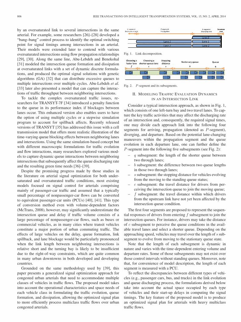
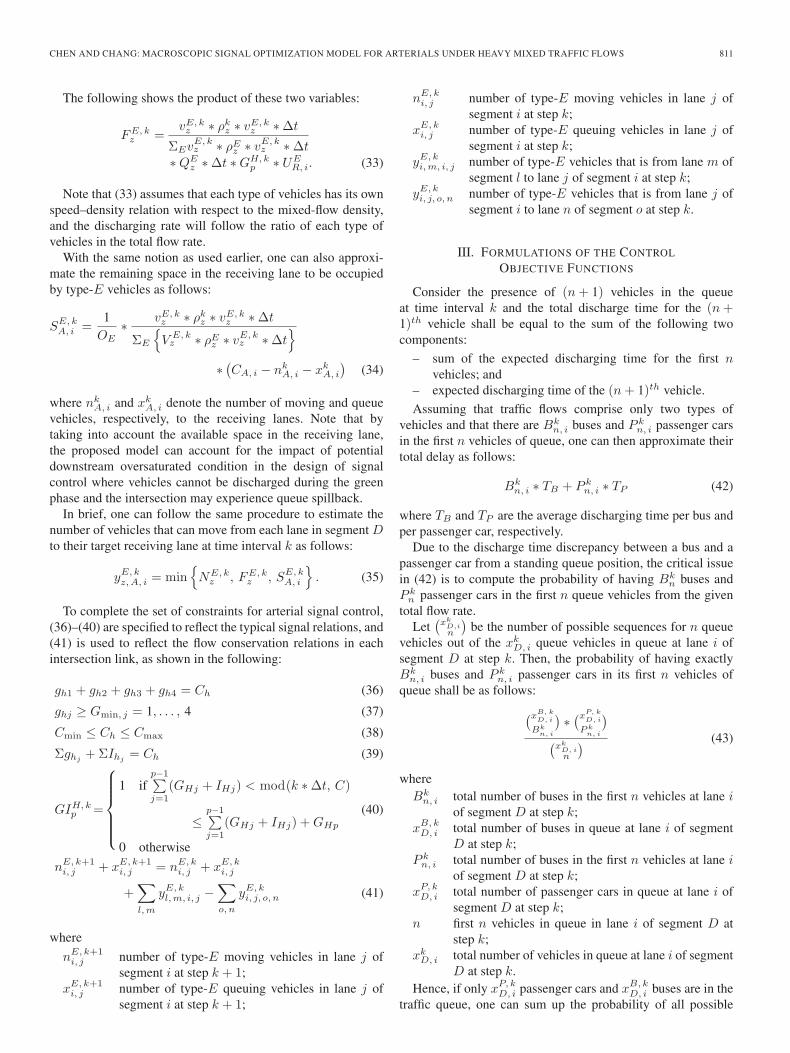
Fig. 1. Link decomposition.

Fig. 2. P -segment and its subsegments.

II. MODELING TRAFFIC EVALUATION DYNAMICS

IN AN INTERSECTION LINK

Consider a typical intersection approach, as shown in Fig. 1,which consists of one left-turn bay and two travel lanes. To cap-ture the key traffic activities that may affect the discharging rateof an intersection and, consequently, the required signal times,one may divide each approach link into the following foursegments for arriving, propagation (denoted as P -segment),diverging, and departure. Based on the potential lane-changingmaneuvers within the propagation segment and the queueevolution in each departure lane, one can further define theP -segment into the following five subsegments (see Fig. 2):

– q subsegment: the length of the shorter queue betweentwo through lanes;

– b subsegment: the difference between two queue lengthsin those two through lanes;

– s subsegment: the stopping distance for vehicles evolvingfrom the moving to the standing queue status;

– c subsegment: the travel distance for drivers from per-ceiving the intersection queue to join the moving queue;

– f subsegment: the travel distance within which driversfrom the upstream link have not yet been affected by theintersection queue condition.

The first four segments are proposed to represent the sequen-tial responses of drivers from entering f subsegment to join theintersection queues. For instance, drivers may take the distanceof c subsegment to perceive the queue conditions in the avail-able travel lanes and select a shorter queue. Depending on theapproaching speed, vehicles may travel over the length of s sub-segment to evolve from moving to the stationary queue state.

Note that the length of each subsegment is dynamic innature and varies with the time-dependent entering volume anddeparture rates. Some of those subsegments may not exist overthose control intervals without standing queues. Moreover, notethat, for convenience of model description, the length of eachsegment is measured with a PCU.

To reflect the discrepancies between different types of vehi-cles (e.g., passenger cars, bus, and trucks) in the link evolutionand queue discharging process, the formulations derived belowtake into account the actual space occupied by each typeof vehicles and their start-up delays in computing the signaltimings. The key feature of the proposed model is to producean optimized signal plan for arterials with heavy multiclasstraffic flows.

CHEN AND CHANG: MACROSCOPIC SIGNAL OPTIMIZATION MODEL FOR ARTERIALS UNDER HEAVY MIXED TRAFFIC FLOWS 807

A. Compute the Arriving Flow Rate From UpstreamU -Segment to P -Segment

Modeling of traffic evolving from entry to departure startsfrom the demand in the arrival segment (i.e., U -segment). LetDE be the total demand of type-E vehicles during the studyperiod; therefore, its flow rate during the kth interval DE,k canbe expressed as follows:

DE,k =

(DE

3600∗Δt

)(1)

where Δt is the duration of one sliced time interval.Note that, depending on the available physical space, some

vehicles from (1) may not be able to move onto P -segmentduring interval k. Moreover, note that subscript “P ” will beremoved from the following formulations to compress thenotation.

Let nki and xk

i denote the number of moving and queuevehicles (measured with the unit of average passenger car),respectively, in lane i of P -segment at step k; and Ci is thetotal storage space in link i of segment P . Then, its remainingspace RSk

i available to accommodate coming vehicles can beshown with

RSki =

(Ci − nk

i − xki

). (2)

Let V Ei represent the ratio of type-E vehicles over the total

entering flow rate, and OE denotes the ratio of the occupiedspace between a type-E vehicle and a passenger car. Then,with the assumption that every vehicle has the same opportunityto share the available space, the remaining space in lane i ofp-segment during the kth interval to be allocated to type-E ve-hicles shall follow its proportion in the total flow rate (i.e., V E

i ),and the resulting number of such vehicles can be approximatedas follows:

SE,ki =

1oE

∗(Ci − nk

i − xki

)∗ V E

i . (3)

Based on the demand from (1) and the available space shownin (3), the actual number of type-E vehicles yE,k

i to move ontolane i of P -segment during the kth interval shall be as follows:

yE,ki = min

{DE,k, SE,k

i

}. (4)

B. Modeling Lane-Changing Maneuvers and Traffic Evolutionin Subsegment b

The second part of the model is to formulate the lane-changing maneuvers for turning and through vehicles in sub-segments b, c, and f , which are based on the following steps.

Estimating Right-Turning Vehicles Within a SubsegmentWhich can Successfully Change Lanes: With the assumptionthat right-turning vehicles within subsegment b shall intendto change to the rightmost lane, each class of vehicles thatcan successfully make such changes depends certainly on itsdemand level and the space available on the target lane.

For the demand level, let xE,k1, b be the total number of

type-E right-turning vehicles queued at lane 1 of subsegment bin P -segment at step k, and RE,R,k

1, b denote the right-turn ratio

out of the total type-E vehicles. Then, the number of thesevehicles, i.e., XE,R,k

1, b , which may have the desire to changelanes, can be expressed as follows:

XE,R,k1, b = xE,k

1, b ∗RE,R,k1, b . (5)

Certainly, depending on the available space in the rightmostlane, some vehicles from (5) may not be able to make necessarylane changes. For convenience of illustration, let lane 1 beassumed to have a longer queue, and the traffic condition inits neighbor lane (i.e., lane 2) is expected to be in a near-moving queue condition. Hence, the average space and timeheadways for vehicles in lane 2 within the b subsegment canbe approximated as follows.

Average space headway in lane 2:

W k2, b =

Lk2, b − ΣE

(nE,k1, b ∗ lE

)ΣEn

E,k1, b

. (6)

Average time headway:

Hk2, b =

1

vk2, b∗W k

2, b (7)

where vk2, b and nE,k1, b are the average speed of all vehicles and

the number of type-E vehicles, respectively, in subsegment b oflane 2; Lk

2, b denotes the total length of subsegment b; and lE isthe average length of a type-E vehicle.

Note that headways in subsegment b of lane 2 are assumedto distribute uniformly because those vehicles are likely in theforced-flow conditions and are ready to stop. Moreover, notethat the resulting average headway (or space headway) may notserve the need of all vehicle types due to the discrepancy in theirvehicle sizes. Hence, the following binary indicator is adoptedto reflect such a discrepancy:

IE, b, k2 =

{1 if Hk

2, b ≥ tE

0 otherwise(8)

where tE denotes the minimum headway needed for type-Evehicles to change lanes.

Based on the assumption that the percentage of each type ofvehicles in the lane-changing flows from lane 1 is proportionalto its distribution in the total flow, one can approximate the ratioof type-E vehicles in the total lane-changing flows from lane 1as follows:

ME,R,k1, b =

RE,R,k1, b ∗ IE, b, k

2

ΣE

(RE,R,k

1, b ∗ IE, b, k2

) (9)

where RE,R,k1, b denotes the ratio of type-E right-turning vehi-

cles over its total flows at subsegment b in lane 1 at step k.Hence, by assuming that all vehicles intending to change

lanes regardless of their differences in size have the sameprobability to occupy the available space in the target lane,then the number of type-E vehicles SE,R,k

2, b allowed to sharethe total remaining space in subsegment b in the target lane at


step k for lane changes can be represented with the followingexpression:

SE,R,k2, b =

1OE

∗ME,R,k1, b ∗

(Ck

2, b − nk2, b

)(10)

where nk2, b and Ck

2, b are the number of existing vehicles andthe total available space, respectively, at subsegment b in lane 2of segment P at step k, and OE is the average length of onetype-E vehicle.

Based on the actual lane-changing demand from (5) andthe available space for such changes from (10), the numberof type-E right-turning vehicles yE, b,R, k

1,2 at subsegment b inlane 1, which can successfully move to lane 2, is naturally theminimum of (10) and (5) as shown in the following:

yE, b,R, k1,2 = min

{XE,R,k

1, b , SE,R,k2, b

}. (11)

If XE,R,k1, b > SE,R,k

2, b , SE,R,k2, b vehicles can successfully

change lanes, and (XE,R,k1, b − SE,R,k

2, b ) vehicles will not beable to make lane changes at step k. Those vehicles may changelanes at the next time step.

Estimating the Through Vehicles Changing From Lane 1 toLane 2: By assuming that the queue length in lane 1 is b feetlonger than its neighboring lane (i.e., lane 2), it is expectedthat some through vehicles may change to lane 2. Hence, onecan follow the same procedures [i.e., (5) –(11)] to approximatethe number of through vehicles by type, i.e., SE,T, k

2, b , thatcan perform the lane changes based on the allocated space asfollows:

SE,T, k2, b =

1OE

∗RE,T, k

1, b ∗ IE, b, k2

ΣE

(RE,T, k

1, b ∗ IE, b, k2

)∗(Ck

2, b − nk2, b − yE, b,R, k

1,2

). (12)

Note that the given equation assumes that right-turning vehi-cles due to the mandatory nature have the high priority to usethe space in the rightmost lane. Similarly, based on the lane-changing demand and available space, the number of type-Ethrough vehicles yE, b, T, k

1,2 that can successfully change to thelane of a shorter queue at interval k can be estimated with thefollowing:

yE, b,T, k1,2 = min

{XE,T, k

1, b , SE,T, k2, b

}. (13)

C. Modeling Lane-Changing Maneuvers and Traffic Evolutionin Subsegments c and f

Estimate Right-Turning Vehicles Making Lane Changes inSubsegment c: As shown in Fig. 2, vehicles entering subseg-ment c are generally able to perceive the queue lengths on thecurrent and neighboring lanes. Assuming that drivers are likelyto change to the lane of shorter queue unless constrained by theturning need, such a demand NE,R,k

1, c by vehicle type naturallyvaries with the following variables:

– the number of type-E moving vehicles at subsegment cin lane 1 of segment P at step k, i.e., nE,k

1, c ;

– the ratio of right-turning type-E vehicles over the totalflows at subsegment c in lane 1 of segment P at step k,i.e., RE,R,k

1, c ;– the probability that the headways at time k in the re-

ceiving lane are larger than the critical gap for type-Evehicles to change lanes, i.e., PE,k

2, c .

The following illustrates their relations with the number oftype-E right-turning moving vehicles NE,R,k

1, c at subsegment cin lane 1 of segment P at step k, which may intend to performlane-changing activities:

NE,R,k1, c = PE,k

2, c ∗ nE,k1, c ∗RE,R,k

1, c (14)

where PE,k2, c = P (T ≥ tE).

Note that vehicles can successfully change lanes only if thereare acceptable gaps in the target lane. A precise modeling ofsuch a lane-changing process is a complex stochastic queuingissue of moving service windows versus time-varying demandand may be excessively tedious for signal control need if theconcerns are mainly on the pretimed cycle length and greentimes. Hence, one can select a proper and simple distributionbased on field data to approximate the probability used in thegiven equation.

By the same procedure for modeling traffic evolution onsubsegment b, one shall first compute the remaining space tobe allocated to different types of right-turning vehicles, whichis (Ck

2, c − nk2, c), where Ck

2, c denotes the total space in lane 2of subsegment c at time interval k, and nk

2, c shows the occupiedlink space during the same interval.

Assuming that each vehicle has the same probability ofsharing the available space, then the total space to be occupiedby type-E right-turning vehicles in lane 1, i.e., NE,R,k

1, c , shouldbe equal approximately to its volume ratio over the total right-turning flow rate. The following shows such an approximation:

SE,R,k2, c =

1OE

∗NE,R,k

1, c

ΣENE,R,k1, c

∗(Ck

2, c − nk2, c

)(15)

where SE,R,k2, c is the number of type-E right-turning vehicles

that are allowed to change to lane 2 based on the allocated linkspace. Hence, the actual number of type-E vehicles yE, c,R, k

1,2

on subsegment c that can successfully change to lane 2 shall bethe minimum of (14) and (15), and be expressed as follows:

yE, c,R, k1,2 = min

{NE,R,k

1, c , SE,R,k2, c

}. (16)

Estimating Lane-Changing Through Vehicles onSubsegment c: Unlike right-turning vehicles, drivers in lane 1may consider changing to lane 2 only if they may encounter ashorter queue. Thus, following the same procedures for turningvehicles, one can approximate the number of through vehiclesNE,T, k

1, c , which may consider lane changes as follows:

NE,T, k1, c = PE,k

2, c ∗ nE,k1, c ∗RE,T, k

1, c ∗ Ic, k1,2 (17)

where

Ic, k1,2 ={

1 if lane 2 has a shorter queue0 otherwise.

(18)


Similarly, by assuming that right-turning vehicles will begiven the priority to change to the rightmost lane (i.e., lane 2),the remaining space for through vehiclesSE,T,k

2,c in subsegment cthat are allowed to change lanes can be approximated as follows:

SE,T, k2, c =

1OE

∗NE,T, k

1, c

ΣENE,T, k1, c

∗(Ck

2, c − nk2, c − yE, c,R, k

1,2

). (19)

By the same token, the number of through vehicles in sub-segment c that can successfully change lanes shall be theminimum of

yE, c,T, k1,2 = min

{NE,T, k

1, c , SE,T, k2, c

}. (20)

Modeling Lane-Changing Maneuvers and Traffic Evolutionin Subsegment f : Since drivers in subsegment f are assumedto behave similarly in subsegments c, except that their lane-changing decisions would be based on increasing the speedrather than reducing the encountered queue. Hence, one canapply the given derivation procedures to approximate the num-ber of vehicles by type in each lane in subsegment f that maychange lanes at each time interval. The binary indicator with(18) should, however, be changed as follows:

If, k1,2 ={

1 if lane 2 has a higher speed0 otherwise.

(21)

D. Modeling of the Traffic Evolution From the Propagation toDiverge Segments

As shown in Fig. 1, the number of vehicles by type thatcan flow out from segment P to the diverging segment Dconceivably depends on the following factors:

– the number of vehicles in segment P ;– the maximum outgoing flow rate from each lane in

segment P ;– the available space in each receiving lanes in segment D

to accommodate different types of vehicles.Note that a potential lane blockage is likely to occur and

needs to be taken into account in computing the outgoing flowrate if the receiving lane in segment D is a turning bay.

Number of Vehicles Available to Move From Segment P toSegment D: Notably, the traffic evolution in lane 1 from thepropagation to diverging segments is more complex than inlane 2 because its neighboring turning bay may experienceoverflow if having an excessive number of left-turning vehicles.Hence, the following derivation starts with the traffic relationsin lane 2.

Since segment P comprises subsegments f , b, and s, it takesthe following time for a vehicle in lane 2 to evolve over theentire segment and move onto the diverging segment D:

TE,k2 =

Lk2, f

vE,k2, f

+Lk2, c

vE,k2, c

+Lk2, b

vE,k2, b

+Lk2, s

vE,k2, s

(22)

whereTE,k2 total travel time through subsegments f , b, and s of

lane 2 at time k;

Lk2, j length of subsegment j in lane 2 of segment P at

step k (j = f, c, b, s);vE,k2, j The average speed of subsegment j in lane 2 of

segment P at step k (j = f, c, b, s).

The last two terms in the given equation will be zero if noqueue exists in both Lanes 1 and 2. For notation compres-sion, let the time-varying travel time in (22) be represented asfollows:

r(k) =

⌊TE,k2

Δt

⌋. (23)

Hence, those vehicles, i.e., yE,k2 entering lane 2 in segment

P between time intervals (k − r(k)) and k, will be too far frommoving into segment D prior to the kth interval. A mathemati-cal expression of those vehicles is shown in the following:

yE,k2 =

k∑t=k−r(k)

yE, t2 . (24)

The following shows the number of type-E vehicles in lane 2eligible to flow into segment D, i.e., NE,k

2 , which equals thesummation of those in the queue xE,k

2 and moving states nE,k2 ,

and less those yE,k2 by (24), as follows:

NE,k2 =

(nE,k2 − yE,k

2 + xE,k2

). (25)

Given these vehicles ready to move into the diverging seg-ment, one can now proceed to analyze the actual numberof vehicles that can be discharged to the receiving lane insegment D.

Note that, to approximate the outgoing flow rates under thegiven mixed-flow density at time k, different types of vehiclesare assumed to travel at different speeds under the same trafficcondition. For example, passenger cars and motorcycles cangenerally move faster than buses in the same arterial link. Thus,given the V E,k

2 ratio of type-E vehicles out of the total mixed-flow density of ρk2 , one can apply a precalibrated speed–densityrelationship to compute the speed of each vehicle type under themixed-flow density as vE,k

2 , and approximate the total potentialoutgoing flow rate for type-E vehicle as (V E,k

2 ∗ ρk2) ∗ vE,k2 .

However, since given the existence of a left-turn bay inthe discharging segment D, only the through and right-turningvehicles will move to its through lane (i.e., lane 2); the numberof type-E vehicles available to move onto lane 2 can be statedas follows:

FE,k2 =

1OE

∗(RE,T, k

2 +RE,R,k2

)∗(V E,k2 ∗ ρk2 ∗ vE,k

2

)∗Δt (26)

where RE,T, k2 and RE,R,k

2 are the through and right-turn ratioof type-E vehicles over the total type-E vehicles in lane 2 ofsegment P at step k; vE,k

2 denotes the average speed of type-Evehicles over the same segment and time interval; and V E,k

2 isthe ratio of type-E vehicles over the total flow in lane 2.


Fig. 3. Discharging process from segment D.

Conceivably, by the same assumption that each type ofvehicles has the same probability to share the available space inthe receiving lane of segment D, the space in the receiving lanefor type-E vehicles should equal their ratio in the total outgoingflow rate, as shown in

JE,k2 =

vE,k2 ∗ ρk2 ∗ vE,k

2 ∗Δt

ΣEvE,k2 ∗ ρk2 ∗ vE,k

2 ∗ δt. (27)

One can then approximate the number of type-E vehicles inlane 2 allowed to move from segment P into segment D, basedon allocated space, at interval k as follows:

SE,k2 =

JE,k2

OE∗(CD,2 − nk

D,2 − xkD,2

)(28)

whereCD,2 storage space of lane 2 in segment D;nkD,2 number of moving vehicles in lane 2 of segment D

at step k;xkD,2 number of queuing vehicles in lane 2 of segment D

at step k.Based on the supply (25), demand (26), and traffic conditions

(28), one can compute the actual number of vehicles in lane 2that can successfully move into the diverging segment D asfollows:

yE,k2,D,2 = min

{NE,k

2 , FE,k2 , Sk

D,2

}. (29)

Note that the given procedures for lane 2 vehicles are appli-cable to approximate the evolution of lane 1 traffic flow, exceptthat their receiving lanes in segment D could be either lane 1 orlane 0, i.e., the left-turn bay (see Fig. 3).

If lane 1 in segment D has been fully occupied by differenttypes of vehicles, the turning bay would not be able to accom-modate any left-turning vehicles. The following is proposed todefine the status of such a blockage:

QkD,1 =

{0 if

(CD,1 − nk

D,1 − xkD,1

)= 0

1 if(CD,1 − nk

D,1 − xkD,1

)> 0

(30)

where QkD,1 is set to zero if lane 1 of segment D has been fully

occupied by through vehicles at interval k. Then, the availablespace for each vehicle type SE,k

1 from lane 1 to the receiving

lanes in segment D can be expressed as the following generalform:

SE,k1 =

JE,k1

OE∗(CD,1 − nk

D,1 − xkD,1

)∗Qk

D,1. (31)

Note that the given formulations assume that the left-turnbay length is sufficiently long to accommodate left-turningvehicles per cycle. Otherwise, the overflows from the left-turnbay may block the through lanes and cause complex mutualblockage issues. Nevertheless, one can still apply the samederivation process [39] to contend with those intersection-queue-blockage-related issues.

Computing the Discharging Flow Rate From Segment D:As shown in Fig. 3, the number of vehicles to be physicallydischarged from each lane in segment D at time interval k tolane i in the receiving link R depends on the following threevariables:

– number of vehicles by type present in each lane insegment D;

– maximum outgoing flow rate of type-E vehicles ineach lane;

– remaining space to be occupied by type-E vehicles in thereceiving lane.

With respect to the total number of vehicles in segment Deligible to discharge to any downstream receiving lane, one canestimate it with the following

NE,kD, z =

(nE,kD, z − yE,k

D, z + xE,kD, z

)∗ UE

R, i,

z = 0, 1, 2(in segment D) (32)

where nE,kD, z and xE,k

D, z are the number of type-E moving andqueue vehicles in lane z of segment D at step k, respectively;yE,kD, z denotes the number of type-E vehicles entering the same

segment between time interval (k − r(k)) and k; and UER, i

denotes the lane usage ratio of lane i in the receiving link Rthat reflects drivers’ preference of taking each availablereceiving lane.

For the maximum number of vehicles by type that can moveout of segment D at time k, it, as discussed previously, wouldbe the product of the following two variables:

– the total number of vehicles that can be discharged fromsegment D during the sliced interval and the signal status,i.e., QE

D,z ∗Δt ∗GH,kp , where QE

D,z is the dischargingrate, and GH,k

p is the green phase indicator (0 or 1) ofphase p at intersection H at step k;

– the ratio of each type of vehicles over the total flowrate in segment D’s discharging flow rate, i.e., (V E,k

D, z ∗ρkD, z ∗ v

E,kD, z ∗Δt)/(

∑E vE,k

D, z ∗ ρED,z ∗ vE,kD, z ∗Δt),

where ρkD, z is the density of lane z (z = 0, 1, 2) in

segment D at step k, and vE,kD, z is the average speed of

type-E vehicles in lane z of segment D at step k.

Again, for notation compression, the subscript denoting seg-ment D is removed from the questions here.


The following shows the product of these two variables:

FE,kz =

vE,kz ∗ ρkz ∗ vE,k

z ∗Δt

ΣEvE,kz ∗ ρEz ∗ vE,k

z ∗Δt∗QE

z ∗Δt ∗GH,kp ∗ UE

R, i. (33)

Note that (33) assumes that each type of vehicles has its ownspeed–density relation with respect to the mixed-flow density,and the discharging rate will follow the ratio of each type ofvehicles in the total flow rate.

With the same notion as used earlier, one can also approxi-mate the remaining space in the receiving lane to be occupiedby type-E vehicles as follows:

SE,kA, i =

1OE

∗ vE,kz ∗ ρkz ∗ vE,k

z ∗Δt

ΣE

{V E,kz ∗ ρEz ∗ vE,k

z ∗Δt}

∗(CA, i − nk

A, i − xkA, i

)(34)

where nkA, i and xk

A, i denote the number of moving and queuevehicles, respectively, to the receiving lanes. Note that bytaking into account the available space in the receiving lane,the proposed model can account for the impact of potentialdownstream oversaturated condition in the design of signalcontrol where vehicles cannot be discharged during the greenphase and the intersection may experience queue spillback.

In brief, one can follow the same procedure to estimate thenumber of vehicles that can move from each lane in segment Dto their target receiving lane at time interval k as follows:

yE,kz,A, i = min

{NE,k

z , FE,kz , SE,k

A, i

}. (35)

To complete the set of constraints for arterial signal control,(36)–(40) are specified to reflect the typical signal relations, and(41) is used to reflect the flow conservation relations in eachintersection link, as shown in the following:

gh1 + gh2 + gh3 + gh4 = Ch (36)

ghj ≥ Gmin, j = 1, . . . , 4 (37)

Cmin ≤ Ch ≤ Cmax (38)

Σghj+ΣIhj

= Ch (39)

GIH,kp =

⎧⎪⎪⎪⎪⎨⎪⎪⎪⎪⎩

1 ifp−1∑j=1

(GHj + IHj) < mod(k ∗Δt, C)

≤p−1∑j=1

(GHj + IHj) +GHp

0 otherwise

(40)

nE,k+1i, j + xE,k+1

i, j = nE,ki, j + xE,k

i, j

+∑l,m

yE,kl,m, i, j −

∑o,n

yE,ki, j, o,n (41)

where

nE,k+1i, j number of type-E moving vehicles in lane j of

segment i at step k + 1;xE,k+1i, j number of type-E queuing vehicles in lane j of

segment i at step k + 1;

nE,ki, j number of type-E moving vehicles in lane j of

segment i at step k;xE,ki, j number of type-E queuing vehicles in lane j of

segment i at step k;yE,ki,m, i, j number of type-E vehicles that is from lane m of

segment l to lane j of segment i at step k;yE,ki, j, o,n number of type-E vehicles that is from lane j of

segment i to lane n of segment o at step k.

III. FORMULATIONS OF THE CONTROL

OBJECTIVE FUNCTIONS

Consider the presence of (n+ 1) vehicles in the queueat time interval k and the total discharge time for the (n+1)th vehicle shall be equal to the sum of the following twocomponents:

– sum of the expected discharging time for the first nvehicles; and

– expected discharging time of the (n+ 1)th vehicle.

Assuming that traffic flows comprise only two types ofvehicles and that there are Bk

n, i buses and P kn, i passenger cars

in the first n vehicles of queue, one can then approximate theirtotal delay as follows:

Bkn, i ∗ TB + P k

n, i ∗ TP (42)

where TB and TP are the average discharging time per bus andper passenger car, respectively.

Due to the discharge time discrepancy between a bus and apassenger car from a standing queue position, the critical issuein (42) is to compute the probability of having Bk

n buses andP kn passenger cars in the first n queue vehicles from the given

total flow rate.Let

(xkD,in

)be the number of possible sequences for n queue

vehicles out of the xkD, i queue vehicles in queue at lane i of

segment D at step k. Then, the probability of having exactlyBk

n, i buses and P kn, i passenger cars in its first n vehicles of

queue shall be as follows:

(xB, kD, i

Bkn, i

)∗(xP, k

D, i

Pkn, i

)(xkD, in

) (43)

whereBk

n, i total number of buses in the first n vehicles at lane iof segment D at step k;

xB,kD, i total number of buses in queue at lane i of segment

D at step k;P kn, i total number of buses in the first n vehicles at lane i

of segment D at step k;xP,kD, i total number of passenger cars in queue at lane i of

segment D at step k;n first n vehicles in queue in lane i of segment D at

step k;xkD, i total number of vehicles in queue at lane i of segment

D at step k.Hence, if only xP,k

D, i passenger cars and xB,kD, i buses are in the

traffic queue, one can sum up the probability of all possible


combinations Bkn to compute the total expected discharging

time of the first n vehicles in the queue as follows:

∑Bk

n

(xB, kD, i

Bkn, i

)∗(xP, k

D, i

Pkn, i

)(xkD, in

) ∗[Bk

n, i ∗ TB + P kn, i ∗ Tp

]. (44)

Since the probability for the (n+ 1)th vehicle to be a bus or apassenger car can be approximated as (xB,k

D,i −Bkn,i)/(x

kD,i−n)

and (xP,kD, i − P k

n, i)/(xkD,i − n), respectively, the additional dis-

charging time needed for the (n+ 1)th vehicle can be shown asfollows:(

xB,kD, i −Bk

n, i

)xkD, i − n

∗ TB +

(xP,kD, i − P k

n, i

)xkD, i − n

∗ Tp. (45)

Thus, the summation of (44) and (45) offers a reasonableapproximation of the required total expected time W k

D, i, n+1

to discharge (n+ 1) queue vehicles at lane i of segment D atstep k.

Since the total delay equals the sum of expected dischargingtimes of all vehicles plus their waiting time at the red phase, onecan show the objective function of minimizing the total delay asfollows:

min∑i

∑k

((∑n

W kD, i,n

)+Δt ∗ IkD, i ∗ xk

i

)(46)

where IkD, i is the red time indicator for lane i in segment D atstep k, and xk

i is the number of queuing vehicles at interval k inlane i.

The alternative objective function of maximizing the totalthroughput is relatively straightforward and can be show with

max∑E,k, i

yE,kD, i,out (47)

where yE,kD, i,out denotes discharged type-E vehicles at lane i in

subsegment D at step k.

IV. SOLUTION ALGORITHM

As in most optimization models for network signals, theformulations for multiple vehicle classes, including both binaryvariables and nonlinear system constraints, are difficult to findin the global optimal solution. To be efficient for use in practice,this paper has applied two heuristic methods and selected theone that yields better signal settings as the solution.

The first one proposed by Yue and Chang [39] is a GA-based method that can produce a reasonably effective solutionafter an extensive experimental process. As shown in Fig. 4, togenerate control parameters that satisfy the signal optimizationconstraints, the proposed heuristic applies the following decod-ing scheme based on the phase structure. First, let NPn be thenumber of phases at intersection n. A total number of NPn + 1fractions will be then generated for the controller at intersectionn from the decomposed binary strings by converting the binarystring to a decimal number and dividing the number by the

Fig. 4. Flowchart of the solution algorithm with the proposed GAmethod [39].

maximum possible decimal number represented by the binarystring. The NPn + 1 fractions are used to code the green timesand cycle length, as shown in the following equations:

Gnp =Gminnp +

⎛⎝C −

∑j∈Pn

Gminnj −

∑j∈Pn

Inj

⎞⎠

∗ λp ∗p∏

j=1

(1 − λj−1),

p = 1, . . . ,NPn − 1; n ∈ SN (48)

Gnp =Gminnp +

⎛⎝C −

∑j∈Pn

Gminnj −

∑j∈Pn

Inj

⎞⎠

∗p∏

j=1

(1 − λj−1),

p = NPn; n ∈ SN (49)

whereCmin, Cmax minimal and maximal cycle lengths;Gmin

np minimal green time for phase p of intersec-tion n;

C common cycle length for the target arterial forthe given period T ;

Gnp green time for phase p at intersection n for thegiven period T ;

Inp intergreen time for phase p at intersection n.The first population of GA will be generated randomly, and

each individual will be decoded to a set of signal timing plansbased on the aforementioned scheme. Then, one can use theproposed network flow model to compute the objective valuefor the given analysis period T . The corresponding fitnessmeasure can be obtained from the objective function value.Based on the fitness evaluation, the crossover and mutationprocedures will be executed and continued until reaching the


Fig. 5. Flowchart of the solution algorithm with the proposed gauzy branch-and-bound method.

stop criterion. Note that such a solution algorithm will firstmaximize the total system throughput and then switch to min-imize the total travel time in the arterial network if the trafficconditions are undersaturated (see Fig. 4). The characteristicsof GA are available from the literature [39].

The second algorithm, as shown in Fig. 5, is a gauzy branch-and-bound method that uses an incremental search method tosequentially identify a better signal setting and cycle length,which is based on a preselected set of initial values and maximalnumber of iterations. With this heuristic, the initial green timesare first set to the minimum green times, and phase index i andintersection index H are set to 1. Then, the initial value of theobjective function can be computed.

The search procedure is to extend the green time of phasei at intersection H at an increment of one second each time,followed by recomputing the new objection function. If the newvalue for the objective function is better than the incumbentone, then the solution will be updated. After updating with thesolution, the algorithm will examine whether the current cycletime has reached its upper bound (the maximum cycle time).The green time of phase i at intersection H will be increasedagain if the current cycle length is below the upper bound. Ifthe upper bound has been reached and the intersection indexdoes not equal the number of intersections, then it will increaseone unit to the intersection index.

If the new value of the objective function is not better than theincumbent objective function value, the algorithm will increasethe green time for another phase at the current intersection. Ifall phases of the current intersection have been calculated, thegreen time of the first phase at the next intersection shall beadded one increment per second. If one of the following ruleshas been matched, the algorithm shall stop the search process.

1) i and H reach the upper bounds of the phase index andthe intersection index, respectively.

Fig. 6. Network of three intersections and 12 approaches for numericalanalysis.

TABLE IKEY MODEL PARAMETERS AND GEOMETRIC CHARACTERISTICS

USED IN THE EXPERIMENTAL SCENARIOS

Fig. 7. Phase settings.

2) Cycle times of all intersections have reached themaximum.

Due to the complex nature of the signal optimization modelfor arterials experiencing multiclass traffic flows, neither solu-tion method can guarantee to reach the global optimal valueafter reaching the preset maximum iteration. Although theproposed solution algorithm cannot guarantee to obtain theglobal optima, our experimental process has identified thatthe following search sequence can yield a better solution:1) starting the search from the highest demand intersectionin a descending order to the one with the lowest demand ina network; and 2) at each intersection, searching from theapproach having the highest inflows in a descending order tothe one with the lowest traffic volume. Hence, the convergedsolutions from both approaches are used to compare with thebenchmark program TRANSYT-7F to evaluate their efficiency


TABLE IIEXPERIMENTAL SCENARIOS FOR MODEL EVALUATION

and effectiveness. Since our experimental results indicate thatthe gauzy branch-and-bound method outperform the GA meth-ods in most scenarios, the following discussion is focused oncomparing the performance between the gauzy branch-and-bound method and TRANSYT-7F.

V. NUMERICAL ANALYSIS

To ensure the effectiveness of the proposed mixed-flowmodel, this paper has conducted a performance comparisonwith TRANSYT-7F under various undersaturated and oversat-urated traffic conditions with and without multiple classes ofvehicles. Note that the performance indicators for comparisoninclude throughput and the average delay in each individualintersection and at the network level. All such results fromeach scenario under both control models are produced fromthe simulation results with CORSIM using the average of15 replications. Each simulation replication runs 1.5 h, and thesimulation results of first 30 min have been removed from theoutput analysis due to the system stability concern. Fig. 6 illus-trates the network of three intersections and 12 approaches fornumerical analysis, where some key experimental parametersand geometric characteristics listed in Table I were based onthe field survey results from the city of Hsinchu, Taiwan. Thephasing plans for these intersections are shown in Fig. 7.

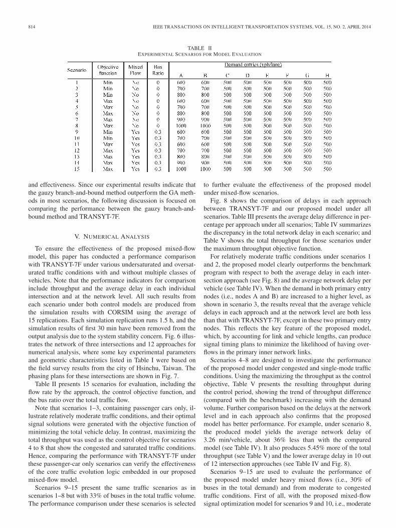
Table II presents 15 scenarios for evaluation, including theflow rate by the approach, the control objective function, andthe bus ratio over the total traffic flow.

Note that scenarios 1–3, containing passenger cars only, il-lustrate relatively moderate traffic conditions, and their optimalsignal solutions were generated with the objective function ofminimizing the total vehicle delay. In contrast, maximizing thetotal throughput was used as the control objective for scenarios4 to 8 that show the congested and saturated traffic conditions.Hence, comparing the performance with TRANSYT-7F underthese passenger-car only scenarios can verify the effectivenessof the core traffic evolution logic embedded in our proposedmixed-flow model.

Scenarios 9–15 present the same traffic scenarios as inscenarios 1–8 but with 33% of buses in the total traffic volume.The performance comparison under these scenarios is selected

to further evaluate the effectiveness of the proposed modelunder mixed-flow scenarios.

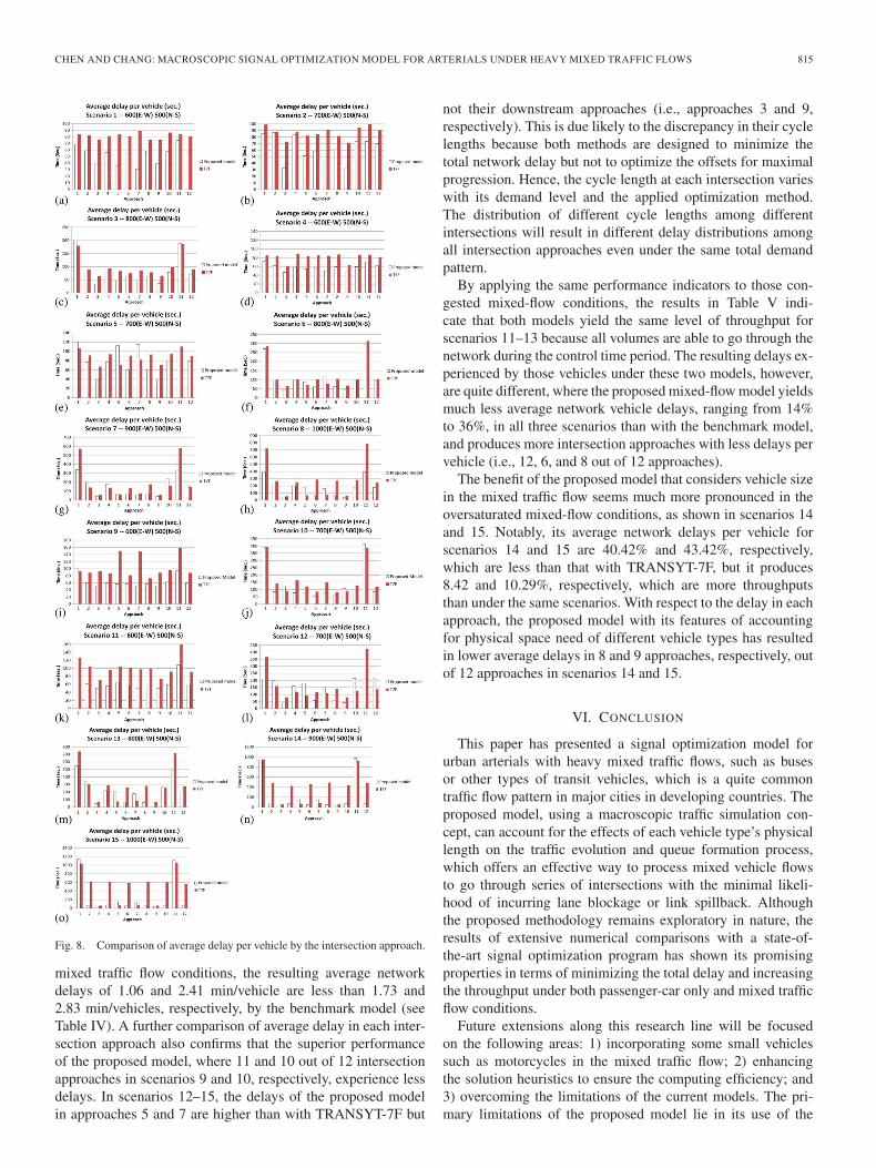
Fig. 8 shows the comparison of delays in each approachbetween TRANSYT-7F and our proposed model under allscenarios. Table III presents the average delay difference in per-centage per approach under all scenarios; Table IV summarizesthe discrepancy in the total network delay in each scenario; andTable V shows the total throughput for those scenarios underthe maximum throughput objective function.

For relatively moderate traffic conditions under scenarios 1and 2, the proposed model clearly outperforms the benchmarkprogram with respect to both the average delay in each inter-section approach (see Fig. 8) and the average network delay pervehicle (see Table IV). When the demand in both primary entrynodes (i.e., nodes A and B) are increased to a higher level, asshown in scenario 3, the results reveal that the average vehicledelays in each approach and at the network level are both lessthan that with TRANSYT-7F, except in these two primary entrynodes. This reflects the key feature of the proposed model,which, by accounting for link and vehicle lengths, can producesignal timing plans to minimize the likelihood of having over-flows in the primary inner network links.

Scenarios 4–8 are designed to investigate the performanceof the proposed model under congested and single-mode trafficconditions. Using the maximizing the throughput as the controlobjective, Table V presents the resulting throughput duringthe control period, showing the trend of throughput difference(compared with the benchmark) increasing with the demandvolume. Further comparison based on the delays at the networklevel and in each approach also confirms that the proposedmodel has better performance. For example, under scenario 8,the produced model yields the average network delay of3.26 min/vehicle, about 36% less than with the comparedmodel (see Table IV). It also produces 5.45% more of the totalthroughput (see Table V) and the lower average delay in 10 outof 12 intersection approaches (see Table IV and Fig. 8).

Scenarios 9–15 are used to evaluate the performance ofthe proposed model under heavy mixed flows (i.e., 30% ofbuses in the total demand) and from moderate to congestedtraffic conditions. First of all, with the proposed mixed-flowsignal optimization model for scenarios 9 and 10, i.e., moderate


Fig. 8. Comparison of average delay per vehicle by the intersection approach.

mixed traffic flow conditions, the resulting average networkdelays of 1.06 and 2.41 min/vehicle are less than 1.73 and2.83 min/vehicles, respectively, by the benchmark model (seeTable IV). A further comparison of average delay in each inter-section approach also confirms that the superior performanceof the proposed model, where 11 and 10 out of 12 intersectionapproaches in scenarios 9 and 10, respectively, experience lessdelays. In scenarios 12–15, the delays of the proposed modelin approaches 5 and 7 are higher than with TRANSYT-7F but

not their downstream approaches (i.e., approaches 3 and 9,respectively). This is due likely to the discrepancy in their cyclelengths because both methods are designed to minimize thetotal network delay but not to optimize the offsets for maximalprogression. Hence, the cycle length at each intersection varieswith its demand level and the applied optimization method.The distribution of different cycle lengths among differentintersections will result in different delay distributions amongall intersection approaches even under the same total demandpattern.

By applying the same performance indicators to those con-gested mixed-flow conditions, the results in Table V indi-cate that both models yield the same level of throughput forscenarios 11–13 because all volumes are able to go through thenetwork during the control time period. The resulting delays ex-perienced by those vehicles under these two models, however,are quite different, where the proposed mixed-flow model yieldsmuch less average network vehicle delays, ranging from 14%to 36%, in all three scenarios than with the benchmark model,and produces more intersection approaches with less delays pervehicle (i.e., 12, 6, and 8 out of 12 approaches).

The benefit of the proposed model that considers vehicle sizein the mixed traffic flow seems much more pronounced in theoversaturated mixed-flow conditions, as shown in scenarios 14and 15. Notably, its average network delays per vehicle forscenarios 14 and 15 are 40.42% and 43.42%, respectively,which are less than that with TRANSYT-7F, but it produces8.42 and 10.29%, respectively, which are more throughputsthan under the same scenarios. With respect to the delay in eachapproach, the proposed model with its features of accountingfor physical space need of different vehicle types has resultedin lower average delays in 8 and 9 approaches, respectively, outof 12 approaches in scenarios 14 and 15.

VI. CONCLUSION

This paper has presented a signal optimization model forurban arterials with heavy mixed traffic flows, such as busesor other types of transit vehicles, which is a quite commontraffic flow pattern in major cities in developing countries. Theproposed model, using a macroscopic traffic simulation con-cept, can account for the effects of each vehicle type’s physicallength on the traffic evolution and queue formation process,which offers an effective way to process mixed vehicle flowsto go through series of intersections with the minimal likeli-hood of incurring lane blockage or link spillback. Althoughthe proposed methodology remains exploratory in nature, theresults of extensive numerical comparisons with a state-of-the-art signal optimization program has shown its promisingproperties in terms of minimizing the total delay and increasingthe throughput under both passenger-car only and mixed trafficflow conditions.

Future extensions along this research line will be focusedon the following areas: 1) incorporating some small vehiclessuch as motorcycles in the mixed traffic flow; 2) enhancingthe solution heuristics to ensure the computing efficiency; and3) overcoming the limitations of the current models. The pri-mary limitations of the proposed model lie in its use of the


TABLE IIIAVERAGE DELAY DIFFERENCE BETWEEN THE PROPOSED AND BENCHMARK MODELS

TABLE IVDIFFERENCE IN THE NETWORK VEHICLE DELAY BETWEEN

THE PROPOSED AND BENCHMARK MODELS

TABLE VHOURLY THROUGHPUT BETWEEN THE PROPOSED

AND BENCHMARK MODELS

average volume from field data as the input, which in reality,could be an interval and vary from day to day. Hence, robustoptimization may be more effective than the currently usedheuristics. Moreover, the assumption that drivers will take themandatory lane change when available, instead of waiting to thelast moment, may not always be consistent with the aggressivedriving patterns. Moreover, the implicit assumption that alldrivers with different vehicle types will behave identically

under the same traffic queue and lane-changing environmentshall be further released in the future work.

REFERENCES

[1] N. H. Gartner, J. D. C. Little, and H. Gabbay, “Optimization of trafficsignal settings by mixed integer linear programming. Part I: The net-work coordination problem,” Transp. Sci., vol. 9, no. 4, pp. 321–343,Nov. 1975.

[2] N. H. Gartner, J. D. C. Little, and H. Gabbay, “Optimization of trafficsignal settings by mixed-integer linear programming Part II: The net-work synchronization problem,” Transp. Sci., vol. 9, no. 4, pp. 344–363,Nov. 1975.

[3] N. H. Gartner, S. F. Assmann, F. Lasaga, and D. L. Hou, “MULTIBAND-Avariable bandwidth arterial progression scheme,” Transp. Res. Rec.,no. 1287, pp. 212–222, 1990.

[4] N. H. Gartner, S. F. Assmann, F. L. Lasaga, and D. L. Hou, “A multi-bandapproach to arterial traffic signal optimization,” Transp. Res. B, vol. 25,no. 1, pp. 55–74, Feb. 1991.

[5] S. L. Cohen and C. C. Liu, “The bandwidth-constrained TRANSYTsignal optimization program,” Transp. Res. Rec., no. 1057, pp. 1–9,1986.

[6] N. A. Chaudhary and C. J. Messer, “PASSER-IV: a program foroptimizing signal timing in grid networks,” Transp. Res. Rec., no. 1421,pp. 82–93, 1993.

[7] C. Stamatiadis and N. H. Gartner, “MULTIBAND-96: A programfor variable bandwidth progression optimization of multiarterial trafficnetworks,” Transp. Res. Rec., no. 1554, pp. 9–17, 1996.

[8] S. C. Wong, “A lane-based optimization method for minimizing delay atisolated signal-controlled junctions,” J. Math. Model. Algorithms, vol. 2,no. 4, pp. 379–406, Dec. 2003.

[9] Q. K. He, K. L. Head, and J. Ding, “PAMSCOD: Platoon-based arterialmulti-modal signal control with online data,” Transp. Res. C, vol. 20,no. 1, pp. 164–184, Feb. 2012.

[10] D. I. Robertson, “TRANSYT: A traffic network study tool,” Road Res.Lab., Berkshire, U.K., RRL Rep. LR 253, 1969.

[11] C. E. Wallace, K. G. Courage, D. P. Reaves, G. W. Shoene, G. W. Euler,and A. Wilbur, TRANSYT-7F User’s Manual. Gainesville, FL, USA:Univ. Florida, 1988.

[12] P. Lowrie, “The Sydney coordinated adaptive control system—Principles,methodology, algorithms,” IEEE Conf. Publication, no. 207, pp. 67–70,1982.

[13] D. I. Robertson and R. D. Bretherton, “Optimizing networks of trafficsignals in real-time: the SCOOT method,” IEEE Trans. Veh. Technol.,vol. 40, no. 1, pp. 11–15, Feb. 1991.

[14] N. H. Gartner, “OPAC: A demand-responsive strategy for traffic signalcontrol,” Transp. Res. Rec., no. 906, pp. 75–81, 1983.

[15] P. Mirchandani and L. Head, “A real-time traffic signal control system:Architecture, algorithms, and analysis,” Transp. Res. C, vol. 9, no. 6,pp. 415–432, Dec. 2001.

[16] M. G. Singh and H. Tamura, “Modeling and hierarchical optimization ofoversaturated urban road traffic networks,” Int. J. Control, vol. 20, no. 6,pp. 913–934, Dec. 1974.


[17] G. C. D’Ans and D. C. Gazis, “Optimal control of oversaturated store andforward transportation networks,” Transp. Sci., vol. 10, no. 1, pp. 1–19,Feb. 1976.

[18] M. Papageorgiou, “An integrated control approach for traffic corridors,”Transp. Res. C, vol. 3, no. 1, pp. 19–30, Feb. 1995.

[19] H. R. Kashani and G. N. Saridis, “Intelligent control for urban trafficsystems,” Automatica, vol. 19, no. 2, pp. 191–197, Mar. 1983.

[20] J. Wu and G. L. Chang, “An integrated optimal control and algorithm forcommuting corridors,” Int. Trans. Oper. Res., vol. 6, no. 1, pp. 39–55,Jan. 1999.

[21] A. Van den Berg, B. Hegyi, De Schutter, and J. Hellendoorn, “A macro-scopic traffic flow model for integrated control of freeway and urbantraffic networks,” in Proc. 42nd IEEE Int. Conf. Decision Control, Maui,HI, USA, 2003, pp. 2774–2779.

[22] X.-H. Yu and W. Recker, “Stochastic adaptive control model for trafficsignal systems,” Transp. Res. C, vol. 14, pp. 263–282, Aug. 2006.

[23] H. Lo, “A novel traffic signal control formulation,” Transp. Res. A, vol. 33,no. 6, pp. 433–448, Aug. 1999.

[24] H. Lo, “A cell-based traffic control formulation: Strategies and benefitsof dynamic timing plans,” Transp. Sci., vol. 35, no. 2, pp. 148–164,May 2001.

[25] C. Beard and A. Ziliaskopoulos, “System optimal signal optimizationformulation,” Transp. Res. Rec., no. 1978, pp. 102–112, 2006.

[26] P. G. Michalopoulos and G. Stephanopolos, “Oversaturated signal sys-tem with queue length constraints—I: Single intersection,” Transp. Res.,vol. 11, no. 6, pp. 413–421, Dec. 1977.

[27] P. G. Michalopoulos and G. Stephanopolos, “Oversaturated signal sys-tems with queue length constraints—II: Systems of intersections,” Transp.Res., vol. 11, no. 6, pp. 423–428, Dec. 1977.

[28] P. G. Michalopoulos and G. Stephanopolos, “Optimal control of oversatu-rated intersections: theoretical and practical considerations,” Traffic Eng.Control, vol. 19, no. 5, pp. 216–221, Jan. 1978.

[29] T. Chang and J.-T. Lin, “Optimal signal timing for an oversaturated inter-section,” Transp. Res. B, vol. 34, no. 6, pp. 471–491, Aug. 2000.

[30] T.-H. Chang and G.-Y. Sun, “Modeling and optimization of an oversat-urated signalized network,” Transp. Res. B, vol. 38, no. 8, pp. 687–707,Sep. 2004.

[31] G. Abu-Lebdeh and R. F. Benekohal, “Development of a traffic and queuemanagement procedure for oversaturated arterials,” Transp. Res. Rec.,no. 1603, pp. 119–127, Dec. 1997.

[32] M. Girianna and R. F. Benekohal, “Using genetic algorithms to designsignal coordination for oversaturated networks,” J. Intell. Transp. Syst.,vol. 8, no. 2, pp. 117–129, Apr. 2004.

[33] G. Abu-Lebdeh, H. Chen, and R. F. Benekohal, “Modeling traffic out-put for design of dynamic multi-cycle control in congested conditions,”J. Intell. Transp. Syst., vol. 11, no. 1, pp. 25–40, Jan. 2007.

[34] M.-T. Li and A. C. Gan, “Signal timing optimization for oversaturated net-works using TRANSYT-7F,” Transportation Research Record, no. 1683,pp. 118–126, 1999.

[35] J. C. Binning, G. Burtenshaw, and M. Crabtree, TRANSYT 13 User Guide.Berkshire, U.K.: Transport Research Laboratory, 2008.

[36] B. Park, C. J. Messer, and T. Urbanik, “Traffic signal optimization pro-gram for oversaturated conditions: Genetic algorithm approach,” Transp.Res. Rec., no. 1683, pp. 133–142, 1999.

[37] I. Yun and B. Park, “Application of stochastic optimization method for anurban corridor,” in Proc. Winter Simul. Conf., 2006, pp. 1493–1499.

[38] A. Stevanovic, P. T. Martin, and J. Stevanovic, “VisSim-based geneticalgorithm optimization of signal timings,” Transp. Res. Rec., no. 2035,pp. 59–68, 2007.

[39] Y. Yue and G.-L. Chang, “An arterial signal optimization model for inter-sections experiencing queue spillback and lane blockage,” Transp. Res. C,vol. 19, no. 1, pp. 130–144, Feb. 2011.

[40] D. Mariagrazia, P. Maria, and C. Meloni, “A signal timing plan formu-lation for urban traffic control,” Control Eng. Pract., vol. 14, no. 11,pp. 1297–1311, Nov. 2006.

[41] Y.-C. Chang and Y.-F. Huang, “Stepwise genetic fuzzy logic signal controlunder mixed traffic conditions,” J. Adv. Transp., vol. 47, no. 1, pp. 43–60,Jan. 2013.

Yen-Yu Chen received the B.S. degree in trafficand transportation management from Feng Chia Uni-versity, Taichung, Taiwan, in 2003 and the M.S.degree in transportation technology and manage-ment from National Chiao Tung University, Hsinchu,Taiwan, in 2005. He is currently working toward thePh.D. degree with the Department of TransportationTechnology and Management, National Chiao TungUniversity.

His current research interests include networktraffic control and advanced traveler information

systems.

Gang-Len Chang (M’13) received the B.Eng. de-gree from National Cheng Kung University, Tainan,Taiwan, in 1975; the M.S. degree from NationalChiao Tung University, Hsinchu, Taiwan, in 1979;and the Ph.D. degree in transportation engineeringfrom the University of Texas at Austin, TX, USA,in 1985.

He is currently a Professor with the Departmentof Civil and Environmental Engineering, Universityof Maryland, College Park, MD, USA. His currentresearch interests include network traffic control,

freeway traffic management and operations, real-time traffic simulation, anddynamic control of urban systems.

Dr. Chang is a member of the American Society of Engineers (ASCE). Hehas served as the Chief Editor for the ASCE Journal of Urban Planning andDevelopment over the past 13 years.

a macroscopic signal optimization model for … macroscopic signal optimization model for arterials...

Documents