A Mathematical Model of the Skype VoIPCongestion Control Algorithm

Luca De Cicco and Saverio Mascolo

Abstract—Voice over Internet Protocol (VoIP) is an Internet applicationof ever increasing importance. The purpose of this note is to derive amathematical model of the Skype VoIP congestion control. The proposedmodel is in the form of a non linear hybrid automaton, which has beenvalidated through extensive experiments. The dynamics of the Skypesending rate, the stability of its equilibrium points and the efficiency inbandwidth utilization while avoiding network instability are analyzed.Results show that, under network congestion, the Skype sending rate isdriven by the packet loss ratio and matches the available bandwidth witha steady state finite error.

Index Terms—Hybrid automaton, Computer networks, VoIP conges-tion control

I. INTRODUCTION

The transport of multimedia traffic over the Internet is of everincreasing importance due to the spreading of multimedia contentdelivery applications such as IP television (IPTV), Videoconferencingover IP, Voice over IP (VoIP), video on demand (VoD).

The stability of the traditional data Internet is due to the Trans-mission Control Protocol (TCP) congestion control algorithm, whichconstitutes the most complex part of the TCP [1]. However, theTCP congestion control is not appropriate to deliver time-sensitivetraffic such as VoIP calls, because of its retransmission mechanismand additive increase multiplicative decrease (AIMD) sliding windowcontrol [2], [3]. As a consequence, audio/video applications employproprietary congestion control algorithms that are executed over theUDP protocol, which is a transport protocol that does not implementcongestion control [2].

Voice over IP is an important example of a real-time serviceincreasingly offered over the Internet. Skype VoIP today countsover 40 millions active users worldwide and up to 17 millionsconcurrent users1. Skype reports that more than 100 billions minutesof calls have been generated by Skype clients, resulting in themost used VoIP application2. Thus, Skype can be considered as themost representative application producing VoIP traffic. This explosivegrowth poses challenges to telecom operators and ISPs both from thepoint of view of network stability and business model. For this reason,it is important to assess the impact of a large number of Skype VoIPcalls on TCP responsive traffic that stills delivers the most part ofthe Internet traffic [2], [3]. In second instance, this study is usefulto understand if there is the need for a better designed congestioncontrol algorithm for VoIP.

Up to now, the only congestion control algorithm for data networksthat has been widely modelled and analyzed is the standard TCPcongestion control and its variants [4],[5],[6],[7],[8]. This is due tothe fact that the TCP congestion control algorithm and its variantsare fully disclosed and well described in scientific literature and instandardization bodies such as the IETF.

The TCP Friendly Rate Control (TFRC) protocol is a new conges-tion control algorithm designed for multimedia flows which is understandardization within the IETF [3]. However, as a matter of fact,

Luca De Cicco is post-doc at Dipartimento di Elettrotecnica ed Elettronica,Politecnico di Bari, Via Orabona 4, Italy (e-mail: ldecicco@gmail.com)

Saverio Mascolo is a Faculty member of Dipartimento di Elettrotecnicaed Elettronica, Politecnico di Bari, Via Orabona 4, Italy (e-mail: mas-colo@poliba.it)

1http://share.skype.com/stats rss.xml2http://ebayinkblog.com/wp-content/uploads/2009/01/skype-fast-facts-q4-

08.pdf

Audio Input Received Audio

rs(t)

SenderSkype

Receiver

RTT (t), l(t)

EmulatedIP NetworkCongestion

Controller

Skype

Measurement

Fig. 1. Experimental testbed emulating a Skype audio call over the Internet

this standardization effort is lagging behind and TFRC is not used inany commercial multimedia application.

The literature regarding Skype can be grouped in three maincategories: 1) studies concerning its peer-to-peer overlay network[9], [10]; 2) studies on its traffic characteristics (see [11], [12] andreferences therein); 3) studies on how to identify Skype calls amongother flows [13].

Authors of [9] present the results of a large-scale experimentalevaluation focusing on the P2P network employed by Skype. Inparticular they focus on the technique employed to implement NATtraversal functionalities and they characterize the super-nodes (SN)of the P2P network.

In [11], [12], we have shown that Skype reacts to networkcongestion by reducing the sending rate, thus being able to matchthe link capacity to some extent.

In [13] the characteristics of Skype VoIP traffic have been studiedand a method to identify Skype calls among other flows has beenproposed. The method is based on two classifiers: one employs theChi-Square test to the payload of passively sniffed traffic, the othermeasures packet size and inter packet gaps.

This paper enriches the literature by proposing for the first timea mathematical model that describes how Skype VoIP dynamicallytracks the network available bandwidth in the presence of variablenetwork conditions. The model can be used to analyze fundamentalproperties of the Skype congestion control such as network stabilityand efficiency in network utilization.

Modelling the sending rate produced by Skype is difficult due tothe following reasons: 1) the protocol behaviour is hidden by AES en-cryption; 2) the input variables that drive the controller are unknown;3) it is very reasonable to conjecture that the controller implementsswitching dynamics due to the use of if-then-else decisional blocks.

The rest of this note is organized as follows: in Section IIwe summarize the data collected through extensive experimentalinvestigations in order to build the model; in Section III we propose amathematical model of Skype sending rate when congestion occurs;in Section IV we derive a hybrid model of a Skype flow accessinga bottleneck link along with a stability analysis. Finally, Section Vdraws the conclusions.

II. EXPERIMENTAL TESTBED AND BACKGROUND

Fig. 1 shows a block diagram of the system to be modelled. Weconsider the Skype sending rate dynamics as the output of a black boxthat models the congestion controller. In [14] we have conjecturedthe following two input variables: 1) the connection round trip time(RTT); 2) the packet loss ratio. To the purpose, it is worth noting thatround trip times and packet loss rates are two variables that can beeasily measured end-to-end to be used as feedback signals in end-to-end congestion control algorithms. In particular, congestion controlalgorithms that employ delay measurements to adjust the input rateare called delay-based (such as in the case of TCP Vegas and TCPFast), whereas algorithms that react to losses are called loss-based(such as in the case of TCP Reno and its variants).

2

NormalS1

LossesS3

CongestionS2

Li(0) = Linit

l(0) = 0

Fig. 2. Skype VoIP hybrid system model

The Skype VoIP sender receives round trip time RTT (t) and lossratio l(t) as feedback variables3 and set the sending rate rs(t) bythrottling both packet size and packet sending rate.

In order to model how feedback signals drive the Skype sendingrate, we have collected data through extensive experimental measure-ments obtained using the testbed shown in Fig. 1, which consists ofreal Skype applications running over a local area network where arouter-host is properly equipped to delay packets, set the availablebandwidth b(t) and set packet drop probability l(t). In particular, wehave considered step-like inputs for RTT (t), l(t) and the availablebandwidth b(t), which is a basic practice when trying to investigatethe dynamic behaviour of a system. The experimental evaluationreported in [14] has led to the following findings: 1) variations of theinput signal RTT (t) have no significant effect on the input rate, thusSkype VoIP does not implement a delay-based congestion control; 2)when the signal l(t) is increased, Skype reacts to a persistent lossby increasing the transmission rate; moreover, in such cases, packetsize is increased, suggesting that Skype employs a Forward ErrorCorrection (FEC) scheme in order to be able to recover lost packets.FEC is a widely employed technique aimed at recovering lost packetsin real-time Internet applications such as VoIP. Basically, the idea isto piggyback redundant information, i.e. the FEC data, on a VoIPpacket in order to be able to recover lost packets. The redundantinformation is obtained by computing the XOR of previously sentVoIP packets [15].

In [14] we have shown that the Skype VoIP sending rate can bemodelled using the hybrid automaton shown in Fig. 2.

In particular, the sending rate can exhibit three different dynamicsdepending on the state Si (i = 1, 2, 3) of the automaton: in the stateS1, which is characterized by normal network conditions, i.e. nocongestion occurs and no losses are present, the sending rate is keptconstant; in the state S2, which is triggered when Skype realizes thatthe network available bandwidth has changed and congestion occurs,the sending rate is throttled by using the congestion control algorithm;in the state S3, which is triggered when losses not due to networkcongestion are present (i.e. due to a lossy link), Skype employs aForward Error Correction (FEC) scheme in order to counteract thelosses attributed to a lossy link. In [14] we have found that the lossratio measured by Skype l(t) is a first-order low passed version ofthe actual loss ratio l(t) experienced by the flow. The time constantof the filter was found to be around 11 s.

In the next Section, we will focus on the behaviour of the SkypeVoIP sending rate in the presence of variations of the availablebandwidth.

3Skype shows measured RTT and loss ratio in its “technical info” tool-tip

0 100 200 300 400 500 600 700 8000

50

100

time (s)

Thr

ough

put (

kb/s

) Sending rate Loss rate Available BW

0 100 200 300 400 500 600 700 8000

50

100

150

time (s)Pac

ket S

endi

ng r

ate

(pac

kets

/s)

0 100 200 300 400 500 600 700 8000

100

200

300

400

500

time (s)

Pac

ket S

ize

(byt

e)

Fig. 3. Sending rate, loss rate, packet sending rate and packet size evolutionin the presence of a square wave available bandwidth of 200 s period

III. THE SKYPE CONGESTION CONTROL MODEL

This Section aims at providing a mathematical model describingthe dynamic behaviour of the Skype sending rate in the presence ofa variable link available bandwidth.

To the purpose, we investigate how the Skype sending rate reactsto sudden changes of available bandwidth. We employ an availablebandwidth that varies as a square wave with maximum value AM =160 kb/s, minimum value Am = 16 kb/s and with a period equal to200 s, which is large enough to show all the transient dynamics.

Fig. 3 shows that Skype decreases the sending rate when the linkcapacity drops from the value AM to the value Am. The Skypeflow takes approximately 40 s to track the available bandwidth duringwhich it experiences a significant loss rate. It can be viewed that,when the available bandwidth drops, the loss rate increases to a peakvalue of 35 kb/s whereas the sending rate reduces to less than 20 kb/sin around 40 s. When the link capacity increases (i.e. at t = 400 s)the input rate ramps up to 90 kb/s, again in around 40 s.

In order to find out the Skype controller dynamics, we havecaptured both packet sizes and packet sending rate over time (seeFig. 3). It can be noticed that the packet sending rate drops in a step-like function when Skype detects congestion, whereas the packet sizeis decreased slowly, resulting in a slow adaptation to the availablebandwidth. In other terms, the most part of Skype congestion controlis performed by throttling the packet sending rate, whereas the packetsize is changed for fine tuning.

Based on the large number of experiments we have run [11],[14], we make the hypothesis that the audio codec employed bySkype is multi-rate so that the encoder can select among N levelsLk = {L1, L2, . . . , LN} with L1 < L2 < · · · < LN . Moreover,we assume that the Skype adaptive codec is able to select the mostappropriate mode according to a metric which is the analogous ofCarrier to Interference ratio (C/I) in the case of Adaptive Multi-RateWide Band (AMR-WB) encoder.

By letting i(t) denote the switching law i(·) : R 7→ {1, . . . , N}and Li(t) the encoder level at time t, we are ready to make the keyhypothesis that the Skype control law for the sending rate is ruledby the following equation:

rs(t) = (1− l(t)) · (1 + f(t))Li(t) (1)

where f : R 7→ [0, 1] ⊂ R models the FEC action, meaning thatwhen f(t) = 0 the FEC action is not active whereas when f(t) = 1

3

00

0.5

1

200 400 600 800 1000 1200 1400

0 200 400 600 800 1000 1200 14000

500

0 200 400 600 800 1000 1200 1400

200

1

0

0.5

1.5

00

50

150

100

400 600 800 1000 1200 1400

Av. BandwidthPredicted thr.Actual thr.P

ack

et s

ize

(by

tes)

Lo

ss r

atio

kb

/sf

(t)

l(t) l(t)

t (s)

Fig. 4. Comparison between the actual and predicted rate using (1)

the FEC action is at maximum. Equation (1) describes the followingbehaviours: when l(t) = 0 (i.e. no congestion occurs) the sendingrate rs(t) is given by Li(t) or (1 + f(t))Li(t) if the FEC is active.When congestion happens (i.e. l(t) 6= 0) the feedback signal reducesthe sending rate of l(t)(1 + f(t))Li(t).

We have run a set of experiments using a square wave availablebandwidth with maximum value of 160 kb/s, a minimum value of16 kb/s with a period of 400 s.

Fig. 4 shows that the packet size is kept roughly constant until thefirst bandwidth increase occurring at t = 400 s. We conjecture thatSkype infers an increase of the available bandwidth by measuringa decrease in both RTT and l(t), which triggers a “probing phase”.Since losses can occur during this phase, Skype activates the FECaction. We conjecture that Skype implements the FEC action bybundling multiple frames in a single packet, so that an increase in theFEC action will turn into a larger packet size [12], [15]. For theseconsiderations, we conjecture the FEC action f(t) shown in Fig. 4,which is proportional to the packet size. Fig. 4 shows that the FECaction is reduced when the filtered loss ratio l(t) reaches zero, andit is turned off later when l(t) is detected not to grow. Moreover, bylooking at the packet size evolution, we infer that the FEC action iskept off during congestion.

Fig. 4 shows both the Skype measured and predicted sending rateusing (1) with a constant value of Li(t) equal to 56 kb/s. This valueis measured at the beginning of the Skype connection when f(t) = 0and l(t) = 0.

Equation (1) nicely predicts the Skype sending rate, both in the caseof presence or absence of congestion, including the large transienttime we have reported before.

In conclusion, the main driver of the Skype sending rate is l(t),which is a low-pass filtered version of the actual loss ratio l(t).Therefore, the dynamics of l(t) affects the sending rate responseto congestion which is somewhat slow.

IV. HYBRID AUTOMATON MODELLING A SKYPE FLOW

ACCESSING A BOTTLENECK

In this Section we propose a hybrid automaton to model a Skypeflow accessing a single bottleneck link characterized by an availablebandwidth b(t), a drop tail queue whose maximum size is qM and around trip time T which is the sum of the delay of the forward pathT1 and the delay of the backward path T2 .

q = 0

Σ1

o = 0q = r − b

˙l = f2

Σ2

q = 0

Σ3

o = 0 o = r − b

r > b

q = 0 r < b

q 6= 0, q 6= qMr ≤ b

q = qM

˙l = f2

˙l = f1

r ≥ b

Fig. 5. The hybrid automaton model H of a Skype flow accessing a droptail queue

The queue dynamics can be modelled by the following differentialequation [16]:

q(t) =

{0

q(t) = 0, r(t) ≤ b(t) orq(t) = qM , r(t) ≥ b(t)

r(t)− b(t) otherwise(2)

where r(t) is the queue input rate. The queue overflow rate o(t) canbe modelled as follows:

o(t) =

{r(t)− b(t) q(t) = qM , r(t) > b(t)0 otherwise

(3)

which means that when the queue is full the exceeding input rater(t)− b(t) is dropped [16].

The dynamic model of the Skype sending rate can be derived from(1) by considering that the feedback signal l(t) is a filtered version ofthe actual packet loss ratio l(t) = o(t)/r(t) measured at the senderafter the backward delay T2. Based upon experiments, we assumethat Skype filters l(t− T2) using a first order low pass filter with atime constant τ :

˙l(t) = − 1

τl(t) +

1

τl(t− T2)

which, by considering that l(t) = o(t)/r(t), turns out:

˙l(t) = − 1

τl(t) +

1

τ

o(t− T2)

r(t− T2)(4)

By substituting (1) and (3) in (4), after straightforward computa-tions we obtain:

˙l(t) =

f1 = 1−l(t)τ− b(t−T2)/τ

(1−l(t−T2))(1+f(t−T2))Li(t−T2)

q = qM ,

r > b

f2 = − 1τl(t) otherwise

(5)It is simple to show that the dynamics of the considered system canbe described by means of the three states hybrid automaton H whichis shown in Fig. 5.

Let X = {l, q : 0 ≤ l ≤ 1, 0 ≤ q ≤ qM} ⊂ R2 be the set ofcontinuous states, x(t) = [l(t) q(t)]T ∈ X be the continuousstate of the system at the continuous time t and Σ = {Σ1,Σ2,Σ3}denote the discrete set of H [17]. In particular: the state Σ1 holdswhen the queue is empty and the input rate is less then or equalto the link available bandwidth; the system dynamics is describedby state Σ2 when the queue is neither full nor empty; the state Σ3

describes the evolution of the system when the queue is full and theinput rate is greater than or equal to the available bandwidth [16].By considering the guard conditions (r > b and r < b) the domains(or invariant sets) of the three discrete states are the following:

Dom(Σ1) = {x ∈ X|q = 0 ∧ 1− b

(1 + f)Li≤ l ≤ 1}

Dom(Σ3) = {x ∈ X|q = qM ∧ 0 ≤ l ≤ 1− b

(1 + f)Li}

Dom(Σ2) = X\ (Dom(Σ1) ∪Dom(Σ3))

4

In the sequel we will prove four lemmas that will be used toanalyze the stability of the equilibrium points of the automaton H.

Before starting to prove the first Lemma, we notice that the filtertime constant τ ∼= 11 s is from 10 up to 100 times the valueof the RTT measured in realistic Internet scenario, which goesfrom milliseconds up to few seconds such as in the case of oldwireless GPRS networks or satellite connections. Moreover, ITU-T recommends a maximum value of 400 ms for mouth-to-ear delay[18], which corresponds to a round trip time of 800 ms, in orderto consider the quality of a VoIP call acceptable. Therefore, sinceτ � T2 it is well justified to neglect the time delay T2 in the modelof the system.

Lemma 1: When the automaton is in the state Σ3, the followinginequality holds:

b(t) ≤ Li(t)(1 + f(t)) (6)

Proof: In the state Σ3, b(t) ≤ r(t) holds. Since r(t) = (1 −l(t))Li(t)(1 + f(t)) ≤ Li(t)(1 + f(t)), the inequality (6) is proved.Thus, if (6) is not verified Dom(Σ3) is an empty set, and Σ3 is notreachable.

Lemma 2: The system Σ3 has a unique asymptotically stableequilibrium point that is feasible:

l∗ = 1−√

b∗L∗(1+f∗)

q∗ = qM(7)

where b∗, L∗, f∗ are the inputs at steady state.Proof: The state Σ3 holds when r(t) ≥ b(t) and the queue is full

(q = qM ), i.e. when congestion occurs. Equation (5) in steady statecondition (i.e. when ˙

l(t) = 0 and q(t) = 0) gives the equilibriumpoint (7) where b∗, L∗ and f∗ are the steady state inputs. Sincefrom Lemma 1 when in Σ3 it holds b∗ ≤ L∗(1 + f∗), it results thatl∗ ∈ [0, 1], i.e. the equilibrium is feasible.

In order to prove the stability of the equilibrium, we employ thedirect Lyapunov method. By using the candidate Lyapunov functionV (l) = 1

2(l− l∗)2 the following derivative of V (l) is obtained after

straightforward computations:

V (l) = − 1

τ

(l − l∗)2(2− l − l∗)

1− l

which is definite negative for all l ∈ [0, 1]. Thus, for the directLyapunov stability criterion the equilibrium l∗ is asymptoticallystable.

Lemma 3: The system Σ1 has a unique equilibrium point:

l∗ = 0q∗ = 0

(8)

which is globally asymptotically stable.Proof: The lemma is proved by observing that Σ1 is a linear

system with one real strictly negative eigenvalue.Lemma 4: The hybrid automaton H has a sink state Σ3 if b∗ <

(1 + f∗)L∗ and a sink state Σ1 if b∗ > (1 + f∗)L∗.Proof: Let us consider the first part of the proposition which

assumes b∗ < (1 + f∗)L∗. The proof starts by showing that forany initial condition (l0, q0) ∈ X , the state dynamics of the hybridautomaton enters the state Σ3 and remains indefinitely in this state,i.e. Σ3 is a sink state. To this purpose we find the reachability set ofH.

Fig. 6 (a) shows that Dom(Σ2) is partitioned in the following twozones depending on the sign of q:

Z1 = {x ∈ X : l < 1− b∗/(1 + f∗)L∗, 0 ≤ q < qM}Z2 = {x ∈ X : l > 1− b∗/(1 + f∗)L∗, 0 < q ≤ qM}

1

q < 0Dom(Σ2)

˙l < 0

r < b

(a)

l∗

(b)

Dom(Σ3)

1Dom(Σ1)Dom(Σ1) l l

q

qM

q

qM

1− b∗

(1+f∗)L∗

P

Z1 Z2

(r > b) (r < b)

Fig. 6. Qualitative phase portrait of the Skype state space model when (a)b∗ < (1 + f∗)L∗ or (b) b∗ ≥ (1 + f∗)L∗

Thus, it results that if r > b, x ∈ Z1 then the queue builds upotherwise x ∈ Z2 and the queue is drained.

It is easy to show that if we initialize H in the state Σ1 (the queueis empty and r < b) then from (5) the state evolution is given by:

l(t) = l0e− tτ

q(t) = 0

where the initial condition is x0 = (l0, 0) ∈ Dom(Σ1). The stateof H remains in Σ1 if r(t) < b(t) (i.e. when l(t) > 1 − b∗/(1 +f∗)L∗). The state switches to Σ2 at the time t12 when the sendingrate matches the available bandwidth, i.e. when r(t12) = b∗:

t12 = −τ log

(1

l0(1− b∗

(1 + f∗)L∗)

)that is positive for each x0 ∈ Dom(Σ1). Thus, we can concludethat if we initialize H in the Σ1 state, the only reachable state is Σ2

after a time t12. Moreover, since the state is now in the region Z1

the queue must build up, so that the only reachable state from Σ2

is now Σ3. Thus, we can conclude that if H is initialized in Σ1 theonly possible evolution of the state is Σ1 → Σ2 → Σ3.

Let us now focus on the states that can be reached by initializingH in Σ2, that is (l0, q0) ∈ Dom(Σ2) = Z1 ∪ Z2. By solving (5),for t > 0 the evolution of the state is given by:

l(t) = l0e− tτ (9)

q(t) = q0 − l0τL∗(1 + f∗)(1− e−tτ ) + (L∗(1 + f∗)− b∗)t (10)

It is easy to show that if the initial condition belongs to Z1, there isno way for the state to end in Σ1 (since the queue must build up) sothat the only state that can be reached is Σ3 (full queue). Let us nowstart from the initial condition in Z2. Now two different evolutionsof the hybrid automaton are possible: the state can either go in Σ1,then back to Σ2 and then to Σ3, or either go directly in Σ3. Finally,if the initial condition belongs to the set:

P = {x ∈ Z2 : q < τ(L∗(1 + f∗)− b∗) log

(1− b∗

L∗(1 + f∗)

)+ τL∗(1 + f∗)l − τ(L∗(1 + f∗)− b∗)(1 + log l)} ⊂ Z2

the state will follow the path Σ2 → Σ1 → Σ2 → Σ3, otherwiseit will follow the path Σ2 → Σ3. In either the cases if the hybridautomaton starts from Σ2 the state will end in Σ3 that is, the queuefills up and packet losses occur.

In order to conclude the first part of the proof we need to show thatif we initialize the system in Σ3 the state ofH will remain in Σ3. Thisfollows from Lemma 2 since the equilibrium (7) is asymptoticallystable.

5

100

90

80

70

60

50

40

30

20

10

0.1 0.2 0.3 0.4 0.5 0.6 0.7 0.8 0.90 1

q (l∗, q∗) = (0.2546, qM)

l

Fig. 7. Trajectories obtained using the proposed model when L∗ = 54 kb/sand b∗ = 30 kb/s

The second part of the proof which states that Σ1 is a sink stateif b∗ > (1 + f∗)L∗ follows the same arguments we have developedin the first part and it is omitted due to space limitation.

Proposition 1: By considering the equilibrium inputs b∗, L∗ andf∗, the hybrid automaton shown in Fig. 5 reaches the followingasymptotically stable equilibrium state:

l∗ = 1−√

b∗L∗(1+f∗)

q∗ = qM(11)

if b∗ < (1 + f∗)L∗ or:

l∗ = 0; q∗ = 0 (12)

otherwise.Proof: From Lemma 4 we know that if b∗ < (1 + f∗)L∗ then

Σ3 is a sink state, so that for any initial condition (l0, q0) ∈ X thestate ends in Σ3. Moreover, in Lemma 2 we have proved that Σ3 hasthe asymptotic stable equilibrium (11), so that we can conclude thatfor any initial condition (l0, q0) ∈ X the state will asymptoticallyconverge to (11).

If we assume b∗ > (1+f∗)L∗, by following similar arguments, wecan conclude that for any (l0, q0) ∈ X the state will asymptoticallyconverge to (12).Fig. 7 shows the trajectories obtained by considering initial conditions(marked with a ×) (l0, q0) ∈ X . The figure shows that all thetrajectories are attracted by the stable equilibrium (l∗, q∗) predictedby Proposition 1 and marked in Fig. 7 with a ◦.

Proposition 2: Under network congestion, i.e. r∗ > b∗, the Skypecontroller produces a steady state overflow rate equal to:

o∗ =√b∗L∗(1 + f∗)− b∗ (13)

which means that Skype is not able to avoid congestion.Proof: Being in Σ3, Lemma 1 implies b∗ < (1 + f∗)L∗.

From Proposition 1 we know that (11) is an asymptotically stableequilibrium for H. Therefore, by considering (3), the steady statevalue of the overflow rate is given by:

o∗ = (1− l∗)L∗(1 + f∗)− b∗ (14)

Now by substituting (11) in (14), it turns out (13). The overflow rateo∗ is greater than zero since b∗ < L∗(1 + f∗). In other terms, undercongestion, the evolution of the system will be described by Σ3 (see

b(t)

50 100 15000

20

200 250 300 350 400

40

80

60

20

00 50 100 150 200 250 300 350 400

4003503002502001501005000

40

Actual rate

b∗ = 30 kb/s ; L∗ = 56 kb/s

qM

o∗ ∼= 11 kb/s

10

5

q(t)

(KB

)o(

t)(k

b/s)

r(t)

(kb/

s)

t (s)

r∗ ∼= 41 kb/s

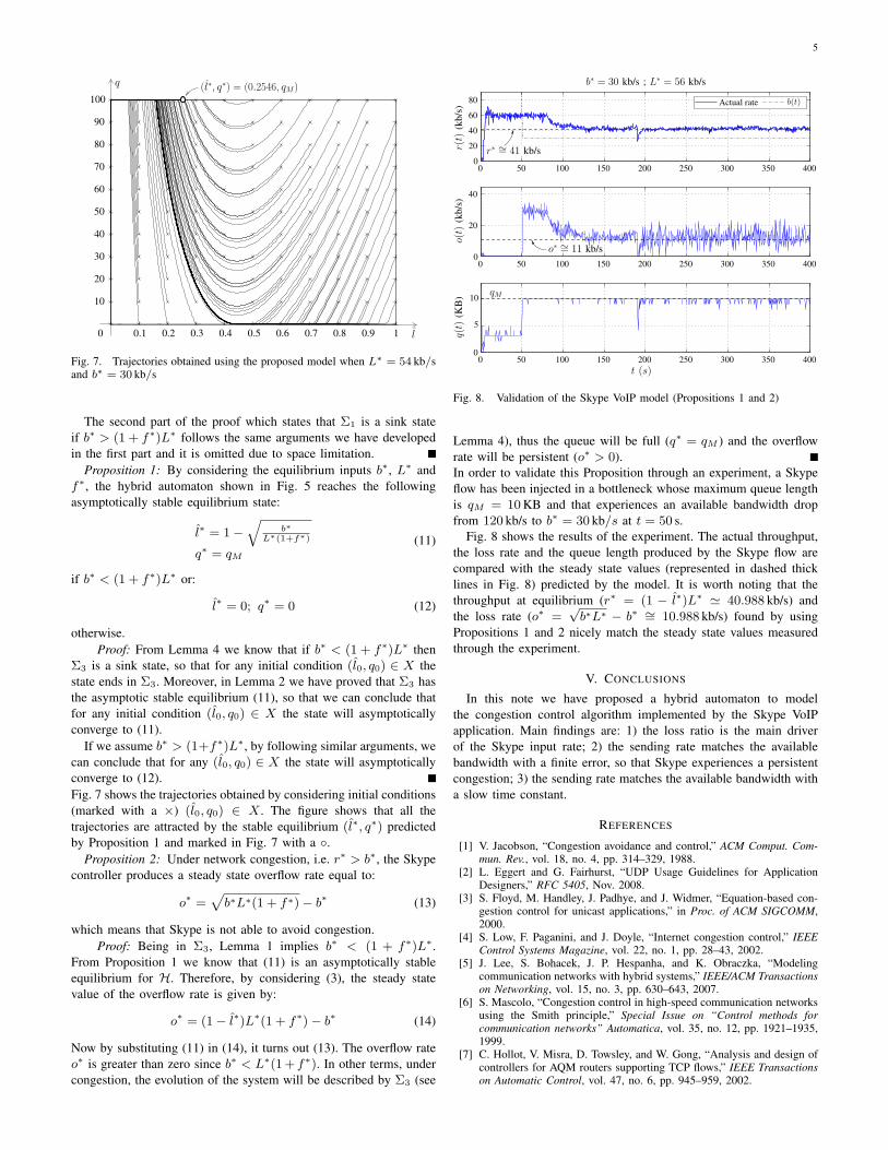
Fig. 8. Validation of the Skype VoIP model (Propositions 1 and 2)

Lemma 4), thus the queue will be full (q∗ = qM ) and the overflowrate will be persistent (o∗ > 0).In order to validate this Proposition through an experiment, a Skypeflow has been injected in a bottleneck whose maximum queue lengthis qM = 10 KB and that experiences an available bandwidth dropfrom 120 kb/s to b∗ = 30 kb/s at t = 50 s.

Fig. 8 shows the results of the experiment. The actual throughput,the loss rate and the queue length produced by the Skype flow arecompared with the steady state values (represented in dashed thicklines in Fig. 8) predicted by the model. It is worth noting that thethroughput at equilibrium (r∗ = (1 − l∗)L∗ ' 40.988 kb/s) andthe loss rate (o∗ =

√b∗L∗ − b∗ ∼= 10.988 kb/s) found by using

Propositions 1 and 2 nicely match the steady state values measuredthrough the experiment.

V. CONCLUSIONS

In this note we have proposed a hybrid automaton to modelthe congestion control algorithm implemented by the Skype VoIPapplication. Main findings are: 1) the loss ratio is the main driverof the Skype input rate; 2) the sending rate matches the availablebandwidth with a finite error, so that Skype experiences a persistentcongestion; 3) the sending rate matches the available bandwidth witha slow time constant.

REFERENCES

[1] V. Jacobson, “Congestion avoidance and control,” ACM Comput. Com-mun. Rev., vol. 18, no. 4, pp. 314–329, 1988.

[2] L. Eggert and G. Fairhurst, “UDP Usage Guidelines for ApplicationDesigners,” RFC 5405, Nov. 2008.

[3] S. Floyd, M. Handley, J. Padhye, and J. Widmer, “Equation-based con-gestion control for unicast applications,” in Proc. of ACM SIGCOMM,2000.

[4] S. Low, F. Paganini, and J. Doyle, “Internet congestion control,” IEEEControl Systems Magazine, vol. 22, no. 1, pp. 28–43, 2002.

[5] J. Lee, S. Bohacek, J. P. Hespanha, and K. Obraczka, “Modelingcommunication networks with hybrid systems,” IEEE/ACM Transactionson Networking, vol. 15, no. 3, pp. 630–643, 2007.

[6] S. Mascolo, “Congestion control in high-speed communication networksusing the Smith principle,” Special Issue on “Control methods forcommunication networks” Automatica, vol. 35, no. 12, pp. 1921–1935,1999.

[7] C. Hollot, V. Misra, D. Towsley, and W. Gong, “Analysis and design ofcontrollers for AQM routers supporting TCP flows,” IEEE Transactionson Automatic Control, vol. 47, no. 6, pp. 945–959, 2002.

6

[8] R. Srikant, The Mathematics of Internet Congestion Control.Birkhauser, 2004.

[9] S. Guha, N. Daswani, and R. Jain, “An Experimental Study of the SkypePeer-to-Peer VoIP System,” in Proc. IPTPS ’06, Feb. 2006.

[10] S. Baset and H. Schulzrinne, “An Analysis of the Skype Peer-to-PeerInternet Telephony Protocol,” in Proc. of IEEE INFOCOM ’06, Apr.2006.

[11] L. De Cicco, S. Mascolo, and V. Palmisano, “An Experimental Investi-gation of the Congestion Control Used by Skype VoIP,” in Proc. of 5thInternational Conference on Wired/Wireless Internet Communications(WWIC), Coimbra, Portugal, May 2007.

[12] ——, “Skype Video Responsiveness to Bandwidth Variations,” in Proc.of ACM NOSSDAV 2008, Braunschweig, Germany, May 28–30, 2008.

[13] D. Bonfiglio, M. Mellia, M. Meo, D. Rossi, and P. Tofanelli, “Revealingskype traffic: when randomness plays with you,” in Proc. of ACMSIGCOMM ’07, Aug. 2007.

[14] L. De Cicco, S. Mascolo, and V. Palmisano, “A Mathematical Modelof the Skype VoIP Congestion Control Algorithm,” in Proc. of IEEEConference on Decision and Control ’08, Cancun, Mexico, 9-11 Dec2008.

[15] W. Jiang and H. Schulzrinne, “Comparison and optimization of packetloss repair methods on voip perceived quality under bursty loss,” in Procof NOSSDAV ’02, Miami, Florida, USA, 2002.

[16] S. Mascolo, “Modeling the Internet congestion control using a Smithcontroller with input shaping,” Control Engineering Practice, vol. 14,no. 4, pp. 425–435, Apr. 2006.

[17] J. Lygeros, K. Johansson, S. Simic, J. Zhang, and S. Sastry, “Dynam-ical properties of hybrid automata,” IEEE Transactions on AutomaticControl, vol. 48, no. 1, pp. 2–17, 2003.

[18] “One-way transmission time,” ITU-T Recommendation G.114, 1993.