a mechanism for the effect of tropospheric jet structure ... · that, for a given subtropical zonal...

A Mechanism for the Effect of Tropospheric Jet Structure on the AnnularMode–Like Response to Stratospheric Forcing

ISLA R. SIMPSON

Department of Physics, University of Toronto, Toronto, Ontario, Canada

MICHAEL BLACKBURN

National Centre for Atmospheric Science, University of Reading, Reading, United Kingdom

JOANNA D. HAIGH

Department of Physics, Imperial College London, London, United Kingdom

(Manuscript received 13 July 2011, in final form 29 January 2012)

ABSTRACT

For many climate forcings the dominant response of the extratropical circulation is a latitudinal shift of the

tropospheric midlatitude jets. The magnitude of this response appears to depend on climatological jet latitude

in general circulation models (GCMs): lower-latitude jets exhibit a larger shift.

The reason for this latitude dependence is investigated for a particular forcing, heating of the equatorial

stratosphere, which shifts the jet poleward. Spinup ensembles with a simplified GCM are used to examine the

evolution of the response for five different jet structures. These differ in the latitude of the eddy-driven jet but

have similar subtropical zonal winds. It is found that lower-latitude jets exhibit a larger response due to

stronger tropospheric eddy–mean flow feedbacks.

A dominant feedback responsible for enhancing the poleward shift is an enhanced equatorward refraction

of the eddies, resulting in an increased momentum flux, poleward of the low-latitude critical line. The sen-

sitivity of feedback strength to jet structure is associated with differences in the coherence of this behavior

across the spectrum of eddy phase speeds. In the configurations used, the higher-latitude jets have a wider

range of critical latitude locations. This reduces the coherence of the momentum flux anomalies associated

with different phase speeds, with low phase speeds opposing the effect of high phase speeds. This suggests

that, for a given subtropical zonal wind strength, the latitude of the eddy-driven jet affects the feedback

through its influence on the width of the region of westerly winds and the range of critical latitudes on the

equatorward flank of the jet.

1. Introduction

The annular modes, which represent migrations in lati-

tude of the tropospheric midlatitude jets, are the dominant

modes of variability in tropospheric zonal mean zonal

wind in both the Northern and Southern Hemispheres

(e.g., Thompson and Wallace 2000; Lorenz and Hartmann

2001, 2003; Kushner 2010). The response to many different

climate forcings also projects strongly onto the annular

modes—for instance, increased anthropogenic emissions

of greenhouse gases (Fyfe and Saenko 2006; Miller

et al. 2006), ozone depletion (Thompson and Solomon

2002), El Nino (Seager et al. 2003), and solar variability

(Haigh et al. 2005, hereafter HBD05). Thus, under-

standing annular mode–like responses is relevant for

understanding many different aspects of climate var-

iability and change.

Although many modeling studies agree on the quali-

tative sense of the response to each of these forcings, it

has recently become apparent that the response mag-

nitude is model dependent. Son et al. (2010) analyzed

the poleward shift of the Southern Hemisphere (SH) jet

in response to ozone depletion in the Chemistry–Climate

Model Validation (CCMVal2) models (SPARC CCMVal

2010). They found considerable variability in the magnitude

Corresponding author address: Isla Simpson, Department of

Physics, University of Toronto, 60 St George St., Toronto, ON M5S

1A7, Canada.

E-mail: [email protected]

2152 J O U R N A L O F T H E A T M O S P H E R I C S C I E N C E S VOLUME 69

DOI: 10.1175/JAS-D-11-0188.1

� 2012 American Meteorological Society

of the zonal wind response, with a near-linear relation-

ship between this and the climatological jet latitude.

Kidston and Gerber (2010) found a similar relation-

ship for the response to increased greenhouse gases.

They compared the magnitude of the poleward shift of

the SH jet between the Coupled Model Intercom-

parison Project (phase 3; CMIP3) models. Again,

a near-linear relationship between the magnitude of

the shift and the climatological jet latitude was found.

The latitude dependence of the response to a forcing

occurs together with a latitude dependence of the

time scale of natural variability (Kidston and Gerber

2010), consistent with the fluctuation–dissipation the-

orem (FDT) (Leith 1975). This joint dependence sug-

gests that, when the midlatitude jet exists at a lower

latitude, the feedbacks between the eddies and the

mean flow are stronger.

The SH midlatitude jet in climate models is generally

biased toward low latitudes relative to observations

(Fyfe and Saenko 2006). Thus, if jet latitude is a major

factor affecting the magnitude of the predicted shift of

the jet in response to a forcing, then models are likely to

be consistently predicting too large a shift in the SH.

Changes in the zonal mean circulation can impact other

aspects of the climate system, such as the uptake of

carbon dioxide by the Southern Ocean (Zickfeld et al.

2007; Lenton et al. 2009; Swart and Fyfe 2011) or sea ice

extent (Sigmond and Fyfe 2010). Thus, biases in the

predicted zonal mean circulation response may signifi-

cantly alter model predictions of both regional-scale and

global climate. It is therefore important to understand

the factors that control the climatological location and

variability of the midlatitude jet and to understand why

the response to a forcing and the time scale of variability

depends on jet structure.

Recently, a great deal of understanding has been

obtained through the use of simplified general circula-

tion models (sGCMs). The advantage of such models is

that they are highly computationally efficient, allowing

long simulations or large ensembles to be performed to

investigate dynamical mechanisms. It has been shown

that the decorrelation time scale of annular mode vari-

ability in sGCMs also depends on the jet latitude (Gerber

and Vallis 2007; Gerber et al. 2008; Son and Lee 2005;

Chan and Plumb 2009; Barnes et al. 2010; Simpson et al.

2010, hereafter SBHS10). In some cases it is found that

simplified GCMs exhibit a bimodality in their jet latitude

such that when the jet exists at a certain location, the

variability is characterized by long time scale transitions

between two preferred jet latitudes (Chan and Plumb

2009). In other cases, a monotonic relationship between

jet latitude and decorrelation time scale is found (SBHS10).

In the sGCM study of SBHS10 it was found that, for the

case of heating of the equatorial stratosphere (which

shifts the jet poleward), the magnitude of the poleward

shift depended on the latitude of the climatological jet,

with lower-latitude jets having a larger response to

forcing than higher-latitude jets. The annular mode

time scale was also longer for lower-latitude jets, con-

sistent with the FDT.

The reason for this joint dependence of both the time

scale of variability and the magnitude of response to a

forcing on the climatological jet latitude in both com-

prehensive and simplified GCMs remains uncertain. Sev-

eral hypotheses have been proposed. One argument is

that the lower-latitude jets are simply able to move

farther poleward before reaching some high-latitude

limit (Kidston and Gerber 2010), although what sets this

high-latitude limit is unclear. Another argument iden-

tifies a difference in the strength of the feedback be-

tween the eddies and the mean flow. Lee et al. (2007)

and Son et al. (2008b) suggest that the dependence of the

time scale of the natural variability on jet latitude in

their sGCM simulations is related to the presence or

absence of a low-latitude reflecting surface. The behav-

ior of the natural variability of the different jet struc-

tures in SBHS10, however, was found to be inconsistent

with this.1 Another possibility, proposed by Barnes et al.

(2010), is that, for lower-latitude jets, the presence of

poleward wave breaking narrows the region of eddy

momentum flux convergence, resulting in a stronger

feedback, whereas higher-latitude jets exhibit a reflect-

ing surface on the poleward side of the jet, no poleward

wave breaking, and a weaker eddy feedback. This is

unlikely to be able to explain the dependence in the

forced runs of SBHS10, where poleward breaking waves

do not appear to play a role in the response or in the

difference in response magnitudes between different

jets and none of the jet structures exhibits a reflecting

surface on the poleward side of the jet (in Fig. 10 of

SBHS10, the refractive index increases to a maximum

on the poleward side of the jet, indicating the presence

of a critical latitude).

The present study follows that of SBHS10 and ad-

dresses the question of why the magnitude of the zonal

wind response depends on jet latitude for a particular

forcing case, heating of the equatorial stratosphere. The

original motivation for this forcing was to represent the

heating of the equatorial lower stratosphere associated

with solar variability. The mechanism involved in

1 SBHS10 incorrectly stated that a subtropical reflecting surface

is present for the most poleward jet (TR5). In fact a critical line

(u 5 c 5 8 m s21) is found before qy

5 0 equatorward of the jet in

all five cases.

JULY 2012 S I M P S O N E T A L . 2153

producing the tropospheric response to this forcing

has already been investigated in detail (HBD05;

Simpson et al. 2009, hereafter SBH09), so it is used

here to investigate the latitude dependence. While

this forcing is different from climate change or ozone

depletion, it acts to shift the jet poleward in a similar

manner. It will be shown that the dependence of the

magnitude of response on jet latitude is related to

the strength of the feedback between the eddies and

the tropospheric zonal wind anomalies and therefore

could be relevant for any forcing that acts to shift

the jet.

The model, experiments, and diagnostics are de-

scribed in section 2. A summary of the experiments

and the results of HBD05, SBH09, and SBHS10 is

given in section 3. The time evolution in response to

stratospheric heating for five different jet structures is

examined in section 4. Section 5 proposes a mecha-

nism for the difference in eddy feedback strength

between the jets, and conclusions will be drawn in

section 6.

2. The model, experiments, and cospectrumanalysis

a. The model

The sGCM used in the following study is the same as

that used in HBD05, SBH09, and SBHS10. It is a spectral

dynamical core as described by Hoskins and Simmons

(1975) with the modification to include the angular mo-

mentum conserving vertical discretization of Simmons and

Burridge (1981) while retaining the original sigma co-

ordinate. Triangular truncation at wavenumber 42 is used

and there are 15 levels between the surface and s 5 0.0185.

Unlike some sGCMs used to investigate stratosphere–

troposphere coupling, the model intentionally does not

include a fully resolved stratosphere and does not exhibit

a stratospheric polar vortex.

The mean state is maintained by Newtonian relaxation

of temperature toward a zonally symmetric equilibrium

state. In the original configuration used in HBD05 and

SBH09, this relaxation temperature distribution is based

on that described by Held and Suarez (1994) and given by

Tref(f, p) 5 max (Ttpeq 2 DTtp sin2f),

�To 2 DTy sin2f 2 (Dueq cos2f 1 Dupl sin2f) log

p

po

� ��p

po

� �� k�,

(1)

where po is the reference surface pressure (51000 hPa),

Ttpeq is the equatorial tropopause temperature, DTtp is

the difference in temperature between the equatorial

and polar tropopause, To is the surface temperature at

the equator, DTy is the difference between the equato-

rial and polar surface temperature, and Dueq and Dupl

are the increase in potential temperature with an in-

crease in altitude of one pressure scale height at the

equator and poles, respectively. In the original Held–

Suarez configuration these parameters are set to Ttpeq

5 200 K, DTtp 5 0 K, To 5 315 K, DTy 5 60 K, Dueq 5

10 K, and Dupl 5 0 K. This relaxation temperature

profile can be seen in Fig. 1c. The temperature is re-

laxed toward this profile on a time scale of 40 days

for s , 0.7 (representing radiation and deep moist

processes), reducing to 4 days at the equatorial surface

(representing the planetary boundary layer). Boundary

layer friction is represented by Rayleigh damping of

winds below s 5 0.7 with a time scale of 1 day at the

surface. The upper boundary condition is reflective (i.e.,

›s/›t 5 0 at the model lid). There is no topography or

other large-scale zonally asymmetric forcing, so plane-

tary waves are weak and are generated only by upscale

energy transfer from the dominant synoptic scales. Bar-

oclinic eddies dominate the wave spectrum with peak

amplitude at zonal wavenumbers 5–7. These are initiated

through a white noise perturbation applied to the surface

pressure at the beginning of each equilibrium integration.

b. The experiments

An advantage of using sGCMs in this Newtonian forced

configuration is that the climatological jet structures can

easily be altered and perturbations can easily be applied by

altering the temperature profile toward which the model

is relaxed. The model experiments that will be examined

in the following are the same as those in SBHS10 but for

completeness they will be described again here.

The response to heating of the equatorial stratosphere

in the model will be examined (the E5 heating case of

HBD05 and SBH09, the letter E referring to equatorial

and 5 referring to the maximum heating of 5 K at the

equator). This heating perturbation is applied by chang-

ing the parameters Ttpeq and DTtp to 205 and 5 K, re-

spectively (see shading in Fig. 1c). It will be applied to five

different tropospheric climatologies, produced by chang-

ing the tropospheric relaxation temperature profile. The

original configuration, denoted TR3, uses the original

Held–Suarez Tref (Fig. 1c). To generate four new tropo-

spheres (TR1, TR2, TR4 and TR5), this original config-

uration is altered by adding the perturbations shown in


FIG. 1. (column1) (c) The Held–Suarez relaxation temperature profile (TR3) (contours) together with the temperature

perturbation that is applied to the stratosphere for the E5 heating case (shading, shading interval 5 0.5 K). (a),(b),(d),(e) The

temperature perturbation added to (c) to create the four tropospheres TR1, TR2, TR4, and TR5, respectively (contour

interval 5 0.5 K). (column 2) Control run horizontal eddy momentum flux for each troposphere (contour interval 5

10 m2 s22). (column 3) Control run zonal wind for each troposphere (contour interval 5 4 m s21). (column 4) Equi-

librium anomaly in zonal wind in response to E5 heating for each troposphere (contour interval 5 1 m s21). Solid and

dotted contours represent positive and negative values, respectively. All panels with the exception of column 2 are

reproduced from SBHS10. The gray regions in column 4 represent 108 latitude bands in the region of maximum zonal

wind decrease and increase that are used later to quantify eddy feedbacks.


Figs. 1a, 1b, 1d, and 1e, and summarized in Table 1, onto

the original Tref.

Midlatitude baroclinicity increases from TR1 to TR5.

TR1 reduces and TR5 enhances the equator to pole

temperature difference by 20 K, by changing the para-

meters To and DTy in Eq. (1) to 305 and 325 K and to 40

and 80 K, respectively. TR2 and TR4 have a different

relaxation temperature profile given by

Tref(f, p) 5 [Eq: (1), rhs]

1 Q cos[2(f 2 p/4)] sin[4(f 2 p/4)]p

po

� �k

,

(2)

where Q is 12 K for TR4 and 22 K for TR2. Therefore,

TR2 has a reduced midlatitude baroclinicity but with the

maximum change in Tref occurring in the subtropics and

subpolar regions. These changes are reversed in TR4.

The five different tropospheric Tref distributions pro-

duce different strengths of eddy fluxes and result in

different strengths and latitudes of the tropospheric jet,

as can be seen in columns 2 and 3 of Fig. 1. The eddy

momentum fluxes increase in strength from TR1 to TR5

and the midlatitude jet strengthens, moves poleward,

and becomes increasingly separated from the subtrop-

ical jet. The responses to equatorial stratospheric heat-

ing shown in SBHS10 are reproduced in column 4 of

Fig. 1 and will be discussed in the following section. These

equilibrium responses are produced from the difference

between a 50 000-day integration with E5 heating ap-

plied and a 50 000-day control run, for each of the five

tropospheres.

The equilibrium response cannot be used to separate

cause and effect due to the presence of strong eddy–mean

flow feedbacks, so spinup ensemble experiments will be

used to examine the time evolution of the response. In

SBHS10, the time evolution of 200 member ensembles

for tropospheres TR2 and TR4 was examined. Here, the

number of ensemble members is increased to 1000 and all

five tropospheres are examined. The 1000 ensemble

members are started from 50-day intervals of the relevant

control integration. Each ensemble member is run for 150

days with the E5 perturbation to Tref continually applied.

In the following, the anomalies over the spinup relative to

the relevant control integration will be examined.

c. The eddy flux cospectra diagnostic

The circulation in midlatitudes is determined by strong

coupling between the zonal mean state and the fluxes of

heat and momentum due to transient synoptic-scale

eddies. The cospectra of these eddy fluxes will be ana-

lyzed, following the method of Hayashi (1971). The eddy

fluxes are calculated from daily instantaneous gridded data

and are separated into contributions over wavenumber–

phase speed (k, c) space at each latitude. Summing over

the zonal wavenumber then allows the eddy fluxes to

be examined as a function of latitude and phase speed.

The refractive properties of the atmosphere, and thus

the direction of eddy propagation, depend on phase

speed (e.g., Matsuno 1970; Karoly and Hoskins 1982), so

it is important to consider how different phase speeds

behave. Randel and Held (1991) demonstrated that,

consistent with linear theory, the momentum fluxes as-

sociated with tropospheric synoptic-scale eddies are re-

stricted to the region between the low- and high-latitude

critical lines (where the zonal mean zonal wind u equals

the phase speed). Moreover, the maximum wave drag

[or Eliassen–Palm (E-P) flux convergence] associated

with the eddies occurs in a region just poleward of the

low-latitude critical line, where the eddies break. Thus,

the distribution of eddy fluxes, and the zonal mean cir-

culation, depends crucially on the eddy phase speed.

Here, the cospectra are analyzed as a function of an-

gular phase speed (cA 5 c/cos f) which is conserved

following waves propagating in the meridional direction

(Randel and Held 1991). When relating momentum

fluxes to critical lines it is therefore necessary to com-

pare cA with u/cosf.

3. An overview of the tropospheric response toequatorial stratospheric heating

The response to the E5 stratospheric heating and its

mechanism have been discussed extensively in HBD05,

SBH09, and SBHS10, so only an overview is given here.

HBD05 found that the equilibrium response for the TR3

tropospheric climatology is a poleward shift of the tro-

pospheric midlatitude jet. SBHS10 showed that the

magnitude of the response depends on the climatologi-

cal jet latitude for the TR1–TR5 climatologies.

The equilibrium responses, reproduced in column 4 of

Fig. 1, comprise a dipole in the zonal mean zonal wind

approximately centered on the jet. The dipole is the sig-

nature of a poleward jet shift, the magnitude of which is

shown in Fig. 2a by the location of maximum zonal wind

in the lower troposphere (675 hPa), so as to describe the

TABLE 1. Summary of the relaxation temperature profiles for the

jet structures TR1–TR5.

Name Tref for the control simulation

TR1 Eq. (1), To 5 305 K, DTy 5 40 K

TR2 Eq. (2), To 5 315 K, DTy 5 60 K, Q 5 2 2 K

TR3 Eq. (1), To 5 315 K, DTy 5 60 K

TR4 Eq. (2), To 5 315 K, DTy 5 60 K, Q 5 2 K

TR5 Eq. (1), To 5 325 K, DTy 5 80 K


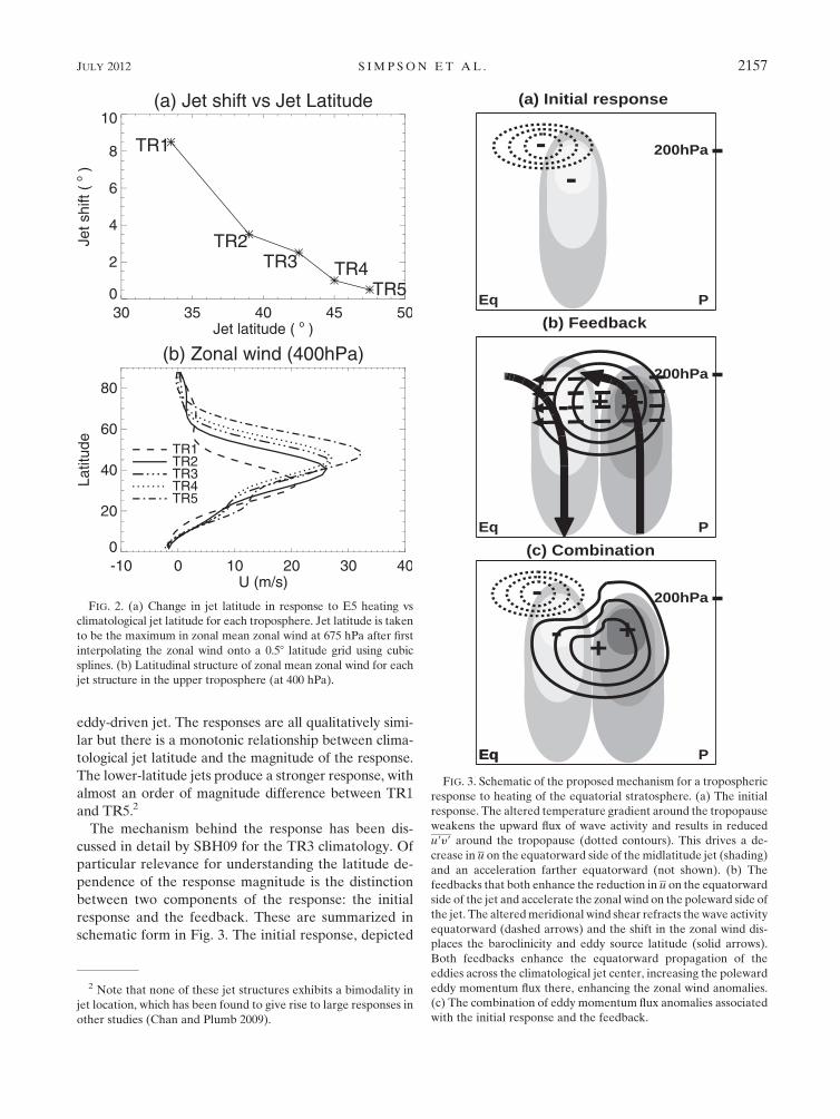
eddy-driven jet. The responses are all qualitatively simi-

lar but there is a monotonic relationship between clima-

tological jet latitude and the magnitude of the response.

The lower-latitude jets produce a stronger response, with

almost an order of magnitude difference between TR1

and TR5.2

The mechanism behind the response has been dis-

cussed in detail by SBH09 for the TR3 climatology. Of

particular relevance for understanding the latitude de-

pendence of the response magnitude is the distinction

between two components of the response: the initial

response and the feedback. These are summarized in

schematic form in Fig. 3. The initial response, depicted

FIG. 2. (a) Change in jet latitude in response to E5 heating vs

climatological jet latitude for each troposphere. Jet latitude is taken

to be the maximum in zonal mean zonal wind at 675 hPa after first

interpolating the zonal wind onto a 0.58 latitude grid using cubic

splines. (b) Latitudinal structure of zonal mean zonal wind for each

jet structure in the upper troposphere (at 400 hPa).

FIG. 3. Schematic of the proposed mechanism for a tropospheric

response to heating of the equatorial stratosphere. (a) The initial

response. The altered temperature gradient around the tropopause

weakens the upward flux of wave activity and results in reduced

u9y9 around the tropopause (dotted contours). This drives a de-

crease in u on the equatorward side of the midlatitude jet (shading)

and an acceleration farther equatorward (not shown). (b) The

feedbacks that both enhance the reduction in u on the equatorward

side of the jet and accelerate the zonal wind on the poleward side of

the jet. The altered meridional wind shear refracts the wave activity

equatorward (dashed arrows) and the shift in the zonal wind dis-

places the baroclinicity and eddy source latitude (solid arrows).

Both feedbacks enhance the equatorward propagation of the

eddies across the climatological jet center, increasing the poleward

eddy momentum flux there, enhancing the zonal wind anomalies.

(c) The combination of eddy momentum flux anomalies associated

with the initial response and the feedback.

2 Note that none of these jet structures exhibits a bimodality in

jet location, which has been found to give rise to large responses in

other studies (Chan and Plumb 2009).


schematically in Fig. 3a, is associated with a lowering of

the tropopause on the equatorward side of the jet, at the

base of the stratospheric heating. This increases the static

stability in that region, which alters the propagation of the

synoptic-scale baroclinic eddies. In the climatology, eddy

growth is centered on the latitude of the jet maximum.

Wave activity propagates upward (associated with a pole-

ward heat flux) and is refracted mainly equatorward

(associated with a poleward momentum flux) consistent

with the behavior of nonlinear baroclinic life cycles (e.g.,

Thorncroft et al. 1993). The increased static stability be-

neath the region of stratospheric warming reduces the up-

ward and equatorward flux of wave activity. The result is

that the wave activity converges slightly lower and closer to

the latitude of the jet. This results in a decrease in poleward

momentum flux around the tropopause, which directly

decelerates the zonal wind on the equatorward side of the

jet around the tropopause and, through the driving of

an anomalous meridional circulation, results in a zonal wind

deceleration lower down in the troposphere.

This initial response triggers a feedback, which consists

of two components depicted schematically in Fig. 3b. In

the first component, the initial zonal wind deceleration

alters the meridional wind shear, which increases the

equatorward refraction of eddies toward the region of

reduced westerly wind. This occurs throughout the upper

half of the troposphere. This increases poleward momen-

tum flux across the jet center, which enhances the initial

deceleration on the equatorward side of the jet and ac-

celerates the zonal wind on the poleward side. These zonal

wind accelerations further increase the meridional wind

shear and equatorward propagation of the eddies, pro-

viding a positive feedback. In the second component of the

feedback, the baroclinicity shifts with the jet, resulting in

an anomalous source of eddy activity on the poleward side

of the jet and a reduced source on the equatorward side.

The momentum fluxes associated with these anomalies in

eddy source provide a further feedback onto the zonal

wind anomalies (Robinson 2000; Kidston et al. 2010).

The equilibrium response, depicted schematically in

Fig. 3c, is a combination of the initial response, which

decelerates the zonal wind on the equatorward side of the

jet, and the feedbacks that enhance that deceleration and

accelerate the zonal wind on the poleward side of the jet.

Thus, the equilibrium eddy momentum flux anomalies

are a combination of decreased momentum flux around

the tropopause in the region of increased stratospheric

temperature on the equatorward side of the jet and in-

creased momentum flux across the jet center. Both of

these anomalies result in an eddy momentum flux di-

vergence on the equatorward side of the jet and the

feedback processes also result in an eddy momentum

flux convergence on the poleward side of the jet.

The questions addressed here are: 1) which of the

above processes leads to the sensitivity of the response

to the climatological jet latitude? and 2) how does this

effect take place?

4. The spinup evolution

a. Evolution of the response

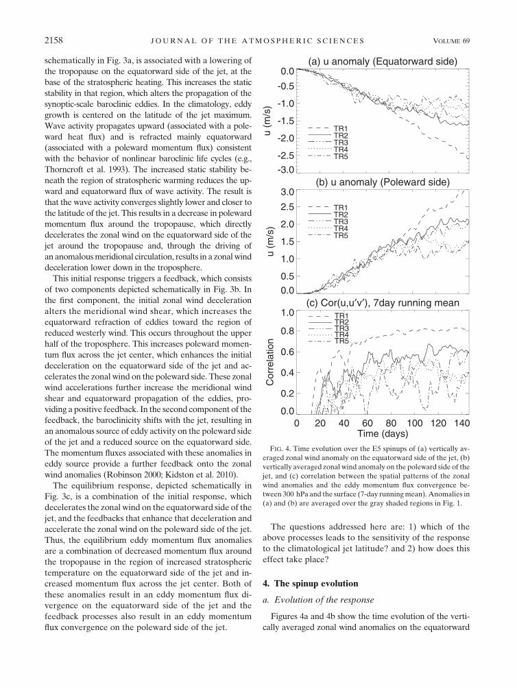
Figures 4a and 4b show the time evolution of the verti-

cally averaged zonal wind anomalies on the equatorward

FIG. 4. Time evolution over the E5 spinups of (a) vertically av-

eraged zonal wind anomaly on the equatorward side of the jet, (b)

vertically averaged zonal wind anomaly on the poleward side of the

jet, and (c) correlation between the spatial patterns of the zonal

wind anomalies and the eddy momentum flux convergence be-

tween 300 hPa and the surface (7-day running mean). Anomalies in

(a) and (b) are averaged over the gray shaded regions in Fig. 1.


and poleward side of the jet. These are averaged over the

gray shaded regions in column 4 of Fig. 1. The data were

first interpolated onto a 0.58 latitude grid using cubic

splines. The locations of the maximum and minimum

zonal wind anomalies at 675 hPa at equilibrium were

obtained and the data were then averaged over the 108

latitude band surrounding those locations. The differ-

ence in zonal wind evolution of each of the tropospheres

becomes clear after about day 80: the zonal wind

anomalies level off and reach equilibrium much sooner

for the higher-latitude jets, while the anomalies for the

lower-latitude jets continue to grow.

Figure 4c provides a measure of the effectiveness of

the eddy momentum flux feedback onto the zonal flow

anomalies in the troposphere. It shows the spatial cor-

relation between the ensemble mean eddy momentum

flux convergence and the zonal wind anomaly over all

latitudes and pressures below 300 hPa after weighting

each field byffiffiffiffiffiffiffiffiffifficosfp

to account for the decrease in area

toward the pole. The correlation is smoothed with a

7-day running mean. The lower the latitude of the eddy-

driven jet, the higher the correlation between the spa-

tial patterns of zonal wind and eddy momentum flux

convergence in the troposphere. This suggests a stronger

tropospheric feedback for the lower-latitude jets. The

correlation for the higher-latitude jets is not only smaller

in magnitude but also more variable in time.

To confirm the role of this difference in eddy feedback

in giving rise to the variation in response between the

different jet structures, the time-integrated momentum

equation will be examined. The Eulerian mean mo-

mentum equation can be written

›u

›t5 f y 2

1

a cos2f

›(u9y9 cos2f)

›f2 ku 1AG, (3)

where overlined and primed quantities represent the

zonal mean and the deviation from the zonal mean, re-

spectively; u and y are the zonal and meridional wind

components; a is the radius of the earth; k is the

boundary layer frictional damping coefficient; and AG

represents the ageostrophic terms. Since the time evo-

lution of spinup anomalies is being investigated here, the

anomaly of each term relative to the relevant control

simulation will be considered.

Equation (3) can be solved for u, as in SBH09, to give

u(t) 2 u(0) 51

ekt

�ðt

0ekt9f y dt9 1

ðt

02ekt9 1

a cos2f

›(u9y9 cos2f)

›fdt9 1

ðt

0ekt9AG dt9

�. (4)

The ekt factors arise from the dependence of the fric-

tional damping on u itself. This time-integrated equation

has the advantage that the evolution of the zonal wind

anomaly is much less noisy than the instantaneous ac-

celeration. The relatively smooth evolution of the zonal

wind can then be attributed to the three different terms:

the Coriolis force acting on the meridional wind, the

momentum flux convergence, and the ageostrophic

terms, each taking account of the frictional damping

below 700 hPa. Above this k 5 0 and the exponential

terms vanish. Thus, the vertical integral of the time-

integrated Coriolis term does not vanish. Its low-level

contribution is reduced by the frictional factor, so the

integral takes the sign of the upper-tropospheric con-

tribution.

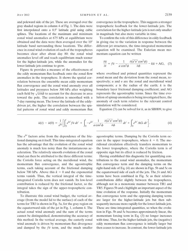
To illustrate this zonal wind budget, the vertical av-

erage (from the model lid to the surface) of each of the

terms for TR3 is shown in Fig. 5a, for the gray region on

the equatorward side of the jet in Fig. 1, column 4. The

actual zonal wind anomaly and the sum of the terms

cannot be distinguished, demonstrating the accuracy of

this method. In the vertical average, the easterly zonal

wind anomaly is driven by momentum flux divergence

and damped by the f y term, and the much smaller

ageostrophic terms. Damping by the Coriolis term oc-

curs in the upper troposphere, where k 5 0. The me-

ridional circulation effectively transfers momentum to

the lower troposphere, where the Coriolis term is of

opposite sign but its effect is reduced by friction.

Having established this diagnostic for quantifying con-

tributions to the zonal wind anomalies, the momentum

flux convergence term and the damping terms on the

right-hand side of Eq. (4) are shown in Figs. 5b and 5c on

the equatorward side of each of the jets. The f y and AG

terms have been combined in Fig. 5c as their relative

contributions differ slightly between the tropospheres,

although not in a monotonic manner between TR1 and

TR5. Figures 5b and c highlight an important aspect of the

time evolution of the response. Initially the momentum

flux convergence term and the opposing damping terms

are larger for the higher-latitude jets but then sub-

sequently increase more rapidly for the lower-latitude jets.

These are time-integrated quantities, so when the evolu-

tion in Figs. 5b and 5c becomes approximately linear, the

momentum forcing term in Eq. (3) no longer increases

with time. Thus, for the higher-latitude jets, the (negative)

eddy momentum flux convergence is initially larger but

then ceases to increase. In contrast, the lower-latitude jets


have an initially smaller momentum flux convergence

anomaly but it continues to increase with time.

b. The initial response and feedbacks

As discussed in section 3, there are two components of

the overall response, an initial response to the strato-

spheric heating and the eddy feedbacks. One way in

which the evolution of the terms in Fig. 5 could be ob-

tained is if the initial response is larger for the higher-

latitude jets but the eddy feedback is weaker. This can be

verified by a more detailed examination of the spatial

patterns of the eddy momentum flux response during two

stages of the spinup: days 0–20, to examine the initial

response, and days 40–70, to examine the feedback stage.

The eddy momentum flux anomalies u9y9 averaged

over days 0–20 are shown for each troposphere in the top

row of Fig. 6. Over the first 20 days, the eddy momentum

flux feedback has not yet become important. Only the

initial response, which consists of a decrease in u9y9

around the tropopause on the equatorward side of the jet,

is apparent (compare with the schematic depiction in Fig.

3a). The initial direct response in temperature above the

tropopause is very similar for each of the jets (not shown;

see SBH09 for the TR3 anomalies), but the momentum

flux response differs. Comparison of Fig. 6, row 1, with

Fig. 1, column 2, shows that the larger response in mo-

mentum flux occurs for the tropospheres with greater

climatological eddy fluxes (i.e., the response increases in

magnitude from TR1 to TR5). This suggests that, for

a given change in tropopause structure, the change in eddy

fluxes is proportional to the climatological eddy fluxes.

The result is that the anomaly in u9y9 divergence (Fig. 6,

row 2) on the equatorward side of the jet increases from

TR1 to TR5, decelerating the higher-latitude jets more

strongly. This can be seen in row 3 of Fig. 6, which shows

the zonal wind anomaly averaged over days 0–20. The

higher-latitude jets, which have stronger climatological

eddy fluxes, therefore have a stronger initial response.

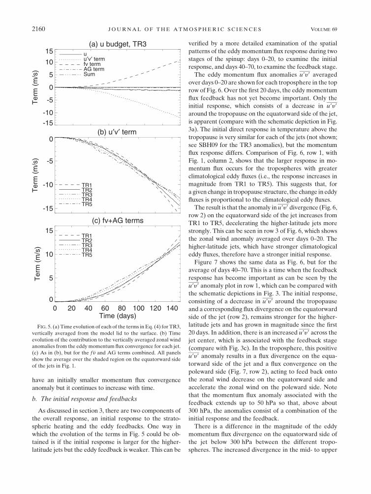
Figure 7 shows the same data as Fig. 6, but for the

average of days 40–70. This is a time when the feedback

response has become important as can be seen by the

u9y9 anomaly plot in row 1, which can be compared with

the schematic depictions in Fig. 3. The initial response,

consisting of a decrease in u9y9 around the tropopause

and a corresponding flux divergence on the equatorward

side of the jet (row 2), remains stronger for the higher-

latitude jets and has grown in magnitude since the first

20 days. In addition, there is an increased u9y9 across the

jet center, which is associated with the feedback stage

(compare with Fig. 3c). In the troposphere, this positive

u9y9 anomaly results in a flux divergence on the equa-

torward side of the jet and a flux convergence on the

poleward side (Fig. 7, row 2), acting to feed back onto

the zonal wind decrease on the equatorward side and

accelerate the zonal wind on the poleward side. Note

that the momentum flux anomaly associated with the

feedback extends up to 50 hPa so that, above about

300 hPa, the anomalies consist of a combination of the

initial response and the feedback.

There is a difference in the magnitude of the eddy

momentum flux divergence on the equatorward side of

the jet below 300 hPa between the different tropo-

spheres. The increased divergence in the mid- to upper

FIG. 5. (a) Time evolution of each of the terms in Eq. (4) for TR3,

vertically averaged from the model lid to the surface. (b) Time

evolution of the contribution to the vertically averaged zonal wind

anomalies from the eddy momentum flux convergence for each jet.

(c) As in (b), but for the f y and AG terms combined. All panels

show the average over the shaded region on the equatorward side

of the jets in Fig. 1.


troposphere is stronger for the lower-latitude jets (cf.

the one negative contour in TR5 with the three negative

contours in TR1 at around 400 hPa in Fig. 7, row 2). This

is associated with a stronger and more meridionally

confined u9y9 anomaly in the troposphere for the lower-

latitude jets (Fig. 7, row 1). This implies that the tro-

pospheric eddy momentum flux feedback onto the zonal

wind decrease on the equatorward side of the jet is

stronger for the lower-latitude jets. It is possible that this

difference in the strength of the eddy feedback could

account for the difference in evolution over the spinup.

A crude method to separate the initial response, oc-

curring above 300 hPa, from the eddy feedbacks, is to

divide the time evolution of the vertically averaged eddy

momentum flux term in the zonal wind budget [Eq. (4);

Fig. 5b] into the contributions from the region between

0 and 300 hPa and the region between 300 hPa and the

surface. While this does not completely separate the

initial response from the feedbacks, since the feedbacks

extend above 300 hPa, it will be shown that it is suffi-

cient to identify the difference in feedback strength as

being the dominant factor that gives rise to the different

equilibrium responses of the jets. For the equatorward

side of the jet, the full vertical average of the term is

repeated in Fig. 8a for comparison. To recap, this time

integration of the eddy momentum flux convergence

term in Eq. (3) demonstrates that the anomaly is initially

larger for the higher-latitude jets but it then ceases to

increase. In contrast, the anomaly is initially smaller for

the lower-latitude jets but it continues to increase with

time. The reason for this behavior is investigated next.

In Fig. 8b it can be seen that the contribution of the

eddy momentum flux convergence to the zonal wind

anomalies on the equatorward side of the jet above

300 hPa is larger for the higher-latitude jets for the en-

tire spinup evolution (i.e., the wrong sense to explain the

difference in final responses). The anomalies here are

dominated by the initial response, consistent with the

discussion in the previous section that the initial re-

sponse is larger for the higher-latitude jets because the

climatological eddy fluxes are stronger. In contrast, the

contribution from the eddy momentum flux convergence

below 300 hPa (Fig. 8c) is much larger for the lower-

latitude jets. Thus the vertically integrated momentum

FIG. 6. Averages over days 0–20 of anomalies in (row 1) horizontal eddy momentum flux (contour interval 5 0.5 m2 s22), (row 2)

horizontal eddy momentum flux convergence (contour interval 5 0.05 m s21 day21), and (row 3) zonal mean zonal wind (contour

interval 5 0.05 m s21). (left to right) Tropospheres TR1–TR5 are shown. The 108 latitude bands on the equatorward and poleward side of

the jet are shaded in gray for comparison in row 2.


flux convergence term in Fig. 8a begins to increase more

rapidly for the lower-latitude jets from days 40 to 70 pre-

dominantly because of a difference that can be identified at

these tropospheric levels (i.e., it is associated with the

feedback).

This same decomposition on the poleward side of the

jet reveals that the tropospheric contribution there only

begins to differ between the tropospheres once the zonal

winds begin to differ significantly, which is after about day

80 (Fig. 4b). This is unlike the term on the equatorward

side of the jet in Figs. 8c and 7, row 2, which differs sig-

nificantly between the tropospheres before day 80.

This zonal wind budget analysis reveals that the tro-

pospheric responses begin to differ because of a difference

in the strength of the eddy feedback on the equatorward

side of the jet. It takes about 80 days before this difference

in feedback strength manifests itself in the zonal wind.

Prior to this the higher-latitude jets have a stronger initial

response to the stratospheric heating that dominates over

their weaker feedback, resulting in a larger zonal wind

response in that initial period. In contrast, the lower-

latitude jets have a weaker initial response but a stronger

feedback. Once the stratospheric heating equilibrates,

the initial response no longer increases, whereas the

feedback response does, until eventually the zonal wind

anomalies become sufficiently large that the surface

friction balances the eddy momentum flux convergence

anomalies. The situation brought about by this particu-

lar forcing and these particular jet structures is some-

what fortuitous, as it means that prior to about day 80

the zonal wind anomalies do not differ significantly be-

tween the tropospheres but the feedback strength does.

This time period therefore provides an opportunity to

understand why the eddy feedbacks differ, before the

zonal wind anomalies themselves differ, which would

itself induce a difference in feedback strength.

5. Why do lower-latitude jets have a stronger eddyfeedback?

In Fig. 7 it can be seen that there is a difference in the

strength of the eddy momentum flux feedback on the

equatorward side of the jet stretching from about 300 to

600 hPa. One of the dominant feedbacks producing this

momentum flux anomaly across the jet center is an in-

creased equatorward refraction associated with the

change in meridional wind shear. However, a difference

in this refraction feedback is unlikely to be able to explain

FIG. 7. As in Fig. 6, but for days 40–70. Contour intervals are u9y9 5 0:5 m2 s22, u9y9 convergence 5 0:05 m s21 day21, and U 5 0.5 m s21.


the difference in this momentum flux anomaly between

the tropospheres, as the wind anomalies and their me-

ridional shears are very similar between the different jets.

The baroclinic component of the eddy feedback in-

volves a shift in eddy source latitude associated with the

decrease in baroclinicity on the equatorward side of the jet

and increase on the poleward side. It is possible that there

is a difference in the baroclinicity of the wind responses.

Eddies grow in the region of high baroclinicity associated

with the jet and, in their nonlinear phase, propagate

mainly equatorward, resulting in a poleward momentum

flux toward their latitude of origin (Fig. 1). This acceler-

ates the zonal wind and, together with the action of sur-

face friction, enhances baroclinicity in the eddy source

region, providing a positive feedback (Robinson 2000;

Chen and Plumb 2009; Kidston et al. 2010). A stronger

baroclinic feedback of the eddies onto the mean flow

would therefore require a larger increase in upward E-P

flux in the region of zonal wind increase and a larger de-

crease in upward E-P flux in the region of zonal wind

decrease.

Figure 9 examines the vertical E-P flux anomalies for

days 40–70. There is very little difference in the magni-

tude of the upward E-P flux anomaly on the poleward

side of the jet. Moreover, the decrease on the equator-

ward side of the jet is stronger and broader for higher-

latitude jets. There is no indication that a difference in

the anomalous eddy growth associated with the jet shift

FIG. 8. The vertically averaged eddy momentum flux convergence term in Eq. (4) that contributes to the zonal wind

anomalies for the (a)2(c) equatorward and (d)2(f) poleward side of the jet. (a),(d) Vertically averaged from the

model lid to the surface; (b),(e) and (c),(f) the contributions from 0 to 300 hPa and 300 hPa to the surface, re-

spectively.


is responsible for the enhanced feedback in TR1

compared to TR5. Rather, it must be some aspect of the

eddy propagation that results in a stronger increase in

eddy momentum flux divergence on the equatorward

side of the jet for lower-latitude jets. To examine this

further the eddy flux cospectra are next analyzed.

Column 1 of Fig. 10 shows the control run u9y9 co-

spectra at 400 hPa for each troposphere. 400 hPa is be-

low the subtropical reduction in u9y9, so it allows the

tropospheric feedback to be analyzed in isolation from

the initial direct response. For all phase speeds, the

maximum flux occurs slightly poleward of the critical

line, as expected from critical layer control of eddy

fluxes (Randel and Held 1991). Furthermore, the

higher-latitude jets, which are also stronger, have

a much greater range of phase speeds and much stronger

eddy fluxes.

Columns 2 and 3 of Fig. 10 examine the anomalies in

u9y9 and u9y9 convergence in response to the E5 heating

calculated over the first 80 days of the spinup (with ta-

pering by a cosine function over the first and last 8 days).

This is the period before the wind anomalies become

significantly different between the tropospheres but

when there is already a noticeable difference in the

tropospheric eddy momentum flux feedback on the

equatorward side of the jet. The main component of the

feedback in the early stage of the spinup is the altered

meridional wind shear acting to enhance the equator-

ward refraction of the eddies. The u9y9 anomalies are

consistent with this. There is an enhanced poleward flux

of momentum at all phase speeds resulting in enhanced

momentum flux divergence just poleward of the low-

latitude critical line.

Column 4 of Fig. 10 shows the wind anomaly averaged

over days 0–80 (dashed) and the eddy momentum flux

convergence anomaly, both output from the model

(solid) and calculated from the cospectra (dotted). The

latter two agree very well and any differences are most

likely associated with the lowest phase speeds not being

resolved by the cospectrum analysis. On the poleward

side of the jet there is very little difference between

the tropospheres. Each shows an increase in u of com-

parable magnitude associated with an enhanced u9y9

convergence also of comparable magnitude. On the

equatorward side of the jet the zonal wind decrease is

also of comparable magnitude between the tropo-

spheres, but it is associated with enhanced momentum

flux divergence that does differ significantly (as was

evident in Figs. 7 and 8). In each of the tropospheres

the momentum flux divergence anomaly is displaced

equatorward of the easterly wind anomaly. However,

for the lower-latitude jets the displacement is smaller,

giving more overlap with the wind anomaly, and the

FIG. 9. Anomaly in vertical E-P flux for each troposphere averaged

over days 40–70. Contour intervals are 105 Pa m2 s22 and solid and

dotted contours represent positive and negative values, respectively.


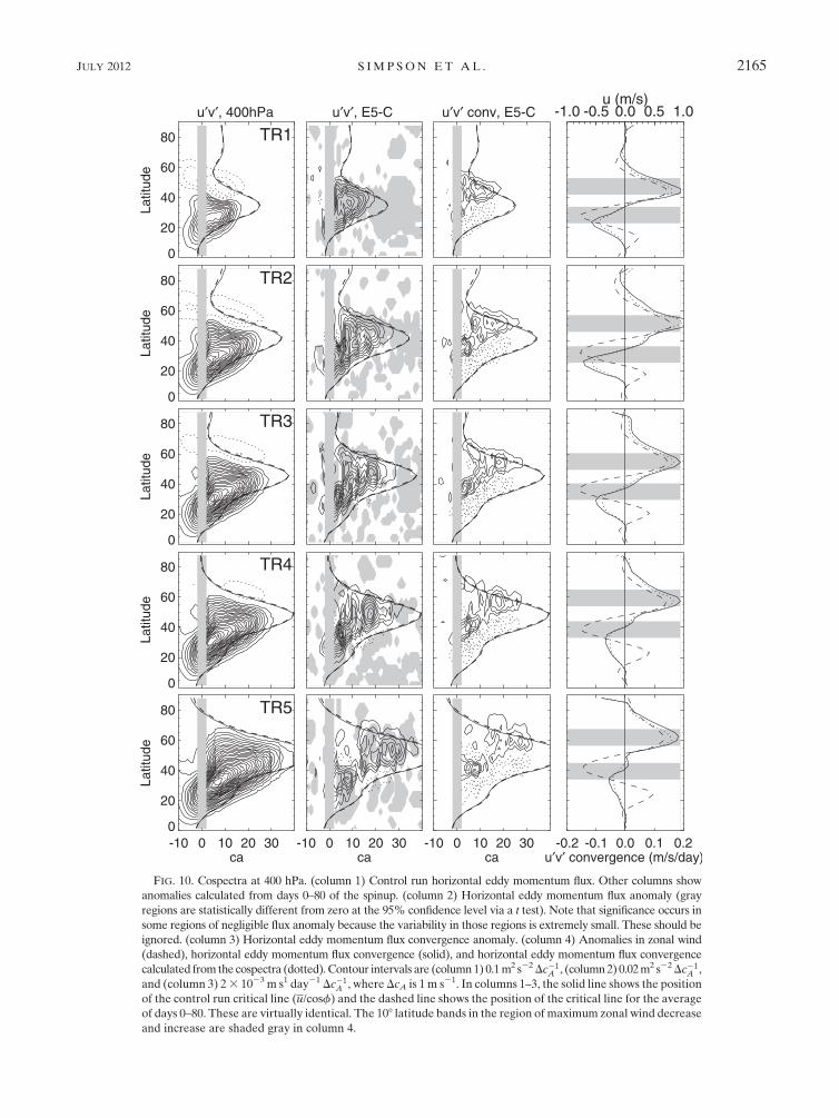
FIG. 10. Cospectra at 400 hPa. (column 1) Control run horizontal eddy momentum flux. Other columns show

anomalies calculated from days 0–80 of the spinup. (column 2) Horizontal eddy momentum flux anomaly (gray

regions are statistically different from zero at the 95% confidence level via a t test). Note that significance occurs in

some regions of negligible flux anomaly because the variability in those regions is extremely small. These should be

ignored. (column 3) Horizontal eddy momentum flux convergence anomaly. (column 4) Anomalies in zonal wind

(dashed), horizontal eddy momentum flux convergence (solid), and horizontal eddy momentum flux convergence

calculated from the cospectra (dotted). Contour intervals are (column 1) 0.1 m2 s22 Dc21A , (column 2) 0.02 m2 s22 Dc21

A ,

and (column 3) 2 3 1023 m s1 day21 Dc21A , where DcA is 1 m s21. In columns 1–3, the solid line shows the position

of the control run critical line (u/cosf) and the dashed line shows the position of the critical line for the average

of days 0–80. These are virtually identical. The 108 latitude bands in the region of maximum zonal wind decrease

and increase are shaded gray in column 4.


momentum flux divergence anomaly is stronger and

sharper. Both these effects result in a stronger eddy

feedback for the lower-latitude jets.

This can be explained by the cospectra of momentum

flux and its divergence in Fig. 10 (columns 2 and 3, re-

spectively). Each phase speed in each troposphere shows

a very similar response, consisting of a dipole with en-

hanced divergence just poleward of the critical line and

enhanced convergence at higher latitudes, as expected

from enhanced equatorward propagation of eddies that

break around the low-latitude critical line. The momen-

tum flux feedback for lower phase speed eddies occurs

consistently close to the subtropical shoulder of the zonal

wind profile for all the jets, just poleward of the low-

latitude critical line for those phase speeds. Figure 2b

shows that the subtropical zonal wind profile is relatively

similar for each of the tropospheres while the midlatitude

jet becomes increasingly separated from the subtropical

westerlies going from TR1 to TR5. The higher-latitude

jets therefore have a greater separation between the low

and high phase speed critical lines. As a result, the low

phase speed eddies fail to feed back positively onto the

equatorward part of the zonal wind dipole, which is al-

ways located close to the midlatitude jet. In fact, the

momentum flux forcing by low phase speed eddies be-

comes more separated from and begins to oppose that of

high phase speed eddies for the more poleward jets,

weakening their positive feedback. Figure 10 shows that,

for TR4 and TR5, this cancellation occurs precisely at the

latitude of the easterly wind anomaly on the equatorward

flank of the jet, with the low phase speeds feeding back

negatively there. The key reason for the larger separation

of the high and low phase speed momentum flux forcings

for higher-latitude jets is the larger separation of their

low-latitude critical lines.

There is little difference between the magnitudes of the

u9y9 convergence anomalies on the poleward side of each

jet. This is because low and high phase speed anomalies in

the high-latitude jets only have different signed anoma-

lies on the equatorward side. In TR5, on the poleward

side of the jet, the convergence due to angular phase

speeds of 10230 m s21 acts in a similar manner to that

due to angular phase speeds of 10220 m s21 in TR1 and

a similar magnitude of convergence results.

6. Discussion and conclusions

A reason has been proposed for the difference in the

magnitude of the poleward shift of the jet in response to

heating of the equatorial stratosphere, based on exami-

nation of the spinup evolution of five different jet struc-

tures. It is found that the main difference in response

between the different jet structures lies in the strength of

the eddy feedback onto the decreased zonal wind on the

equatorward side of the jet.

In the early feedback stages of the spinup, the differ-

ent jet structures differ in the magnitudes of the u9y9

divergence on the equatorward side of the jet associated

with the feedback processes. The u9y9 divergence anom-

aly is narrower and stronger and projects more strongly

onto the zonal wind anomalies for low-latitude jets

compared to high-latitude jets. Thus, the lower-latitude

jets have a stronger feedback between the eddies and the

mean flow, despite having an initially weaker response

(due to their weaker climatological fluxes). This is the

primary reason for the difference in response between

the different jets. Once this effect starts to produce

a larger zonal wind anomaly for the lower-latitude jets,

both the refraction feedback (equatorward propagation

across the jet) and the baroclinic feedback (a poleward

shift of the baroclinicity) become stronger, allowing the

annular mode–like response to heating to grow larger

for the lower-latitude jets.

The key to the difference in the strength of the feed-

back is a difference in the coherence of the behavior

across the spectrum of eddy phase speeds. The higher-

latitude jets used here exhibit a much wider range of

phase speeds and a much wider latitudinal range of crit-

ical latitudes. As a result, different phase speed eddies do

not act together to provide a positive feedback. In fact,

the low phase speed eddies oppose the effect of the high

phase speeds, reducing the deceleration on the equator-

ward side of the jet. This weakens the feedback between

the tropospheric eddy momentum flux and the mean flow

anomalies. The reduced correlation between the spatial

patterns of u9y9 convergence and u anomalies shown in

Fig. 4 is a consequence of this. The increase in u9y9 di-

vergence on the equatorward side of the jet is broader

and weaker for the higher-latitude jets and projects less

well onto the zonal wind reduction on the equatorward

side of the midlatitude jet.

The mechanism for a dependence of the response

magnitude on climatological jet latitude has been pro-

posed here for a particular forcing case. However, it

may be relevant more generally, for example to explain

the similar dependence found by Son et al. (2010) for

polar stratospheric cooling associated with stratospheric

ozone depletion and by Kidston and Gerber (2010) for

anticipated climate change over the twenty-first century,

since the difference between the jet structures lies in the

strength of the tropospheric feedback. Such feedbacks

should occur in response to any forcing that produces an

annular mode–like zonal wind anomaly.

The fluctuation–dissipation theorem (Leith 1975)

predicts that two dominant factors lead to a difference

in the magnitude of an annular mode–like response to


a forcing for different jet structures: 1) the projection of

the forcing onto the annular mode and 2) the time scale

of natural annular mode variability, which depends on

the strength of the feedback between the eddies and the

mean flow. In the experiments reported here, it is the

feedbacks that control the response magnitude. How-

ever, for other forcings, particularly those restricted to

high latitudes, the projection onto the annular mode may

be significantly reduced in the case of lower-latitude jets,

counteracting the tendency for those jets to exhibit

a stronger eddy feedback. In fact, SBHS10 found that an

equatorward jet shift in response to polar stratospheric

heating was also dependent on jet latitude, but that the

sensitivity was less pronounced than for the poleward shift

in response to equatorial heating.

Throughout this study, the discussion has been focused

on an explanation of why there is a dependence on jet

latitude of the response to forcings. However, the mech-

anism proposed actually suggests that the latitudinal range

of critical latitudes on the equatorward side of the jet is

key in determining the feedback strength. By construction

each of these zonal wind structures has relatively similar

subtropical westerly winds (Fig. 2b), so when the eddy-

driven jet is at a higher latitude, the overall region of

westerly winds is wider and a wider latitudinal range of

critical latitudes exists on the equatorward side of the jet.

This would also be true of the real atmosphere in seasons

when the subtropical jet is present. Note that the sub-

tropical zonal winds in TR1 are slightly farther poleward

than those of all the other jets, narrowing the region of

westerlies and enhancing the feedback even further for

that troposphere.

The lower-latitude jets studied here are also weaker. If

the lower-latitude jet was stronger, or the higher-

latitude jet was weaker, then the difference in eddy

feedback would be altered due to the greater or smaller

range of phase speeds present. Based on the hypothesis in

this study alone, one might expect that the stronger and

narrower the jet, the stronger the eddy feedback and

the larger the response. However, there is evidence

from other studies that when the midlatitude jet be-

comes merged with the subtropical jet, such that there

is a single strong jet, the strength of the eddy–mean

flow feedbacks actually decrease (Eichelberger and

Hartmann 2007; Barnes and Hartmann 2011). Eichelberger

and Hartmann (2007) suggest that this is because a

strong jet acts as a waveguide that inhibits the meridi-

onal propagation of waves away from their source lati-

tude, resulting in a weakened eddy–mean flow feedback.

Therefore, there may be other regimes to consider and

it is possible that, within these, a strong, lower-latitude

jet might exhibit a weaker response, but this remains to

be tested.

Another mechanism that has been proposed for pro-

ducing a poleward shift of the midlatitude jets in re-

sponse to a forcing is through a change in the eddy phase

speed. Chen et al. (2007) demonstrated that, in response

to a reduction in surface friction in an sGCM, the phase

speed of the dominant eddies increases. The relevant

critical latitudes are therefore farther poleward so that

a poleward shift of the horizontal eddy momentum flux

results. While this is rather different from the case of

stratospheric heating, as the zonal wind is initially al-

tered at low levels, it has been proposed that altered

vertical wind shear around the tropopause in response to

stratospheric temperature perturbations could also act

to increase the eddy phase speed and cause a shift in the

jet (Chen and Held 2007), but this remains under debate

(e.g., McLandress et al. 2010).

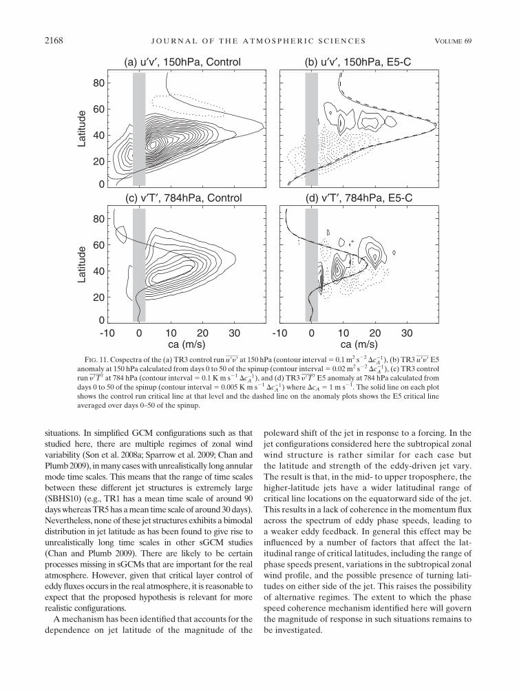
Eddy flux cospectra allow us to examine this for the

case of E5 heating, which induces an increase in lower-

stratospheric zonal wind at mid- to high latitudes (See

Fig. 1 of SBH09). By the Chen et al. (2007) hypothesis,

this could induce a change in the phase speed to produce

the initial response. Figures 11a and 11b show, for the

case of TR3, the control climatology and the anomaly

for the average over days 0–50 of the spinup in the u9y9

cospectra at 150 hPa (i.e., the level at which the initial

decrease in u9y9 occurs). The dominant component of

the initial response is a reduction of the climatological

u9y9 on the equatorward side of the jet at all phase

speeds rather than an increase in the momentum flux at

high phase speeds at the expense of low phase speeds.

The increase in u9y9 on the poleward side of the jet is a

signature of the start of the positive feedback associated

with the equatorward refraction. Furthermore, Figs. 11c

and 11d show the control and early spinup anomaly of the

heat flux y9T9 at 784 hPa to examine sources of anomalous

eddy activity. There is a poleward shift rather than a clear

dipole in phase speed, as found in Fig. 7 of Chen et al.

(2007). The initial reduction in climatological momentum

flux around the tropopause that triggers the tropospheric

response does not appear to be related to anomalies in the

eddy source (neither phase speed nor some other aspect of

eddy generation). It remains to be seen whether other

forcings such as ozone depletion, which may have a

greater effect on the jet speed in the upper troposphere,

act through this phase speed mechanism. However, these

results do show that a change in lower-stratospheric

temperature can trigger a change in the jet position

through the influence of altered static stability around

the tropopause on eddy propagation, rather than through

changes occurring at the eddy source. Such an effect may

also be important for the response to ozone depletion.

It remains to be confirmed whether the results of this

simplified GCM study are relevant for more realistic


situations. In simplified GCM configurations such as that

studied here, there are multiple regimes of zonal wind

variability (Son et al. 2008a; Sparrow et al. 2009; Chan and

Plumb 2009), in many cases with unrealistically long annular

mode time scales. This means that the range of time scales

between these different jet structures is extremely large

(SBHS10) (e.g., TR1 has a mean time scale of around 90

days whereas TR5 has a mean time scale of around 30 days).

Nevertheless, none of these jet structures exhibits a bimodal

distribution in jet latitude as has been found to give rise to

unrealistically long time scales in other sGCM studies

(Chan and Plumb 2009). There are likely to be certain

processes missing in sGCMs that are important for the real

atmosphere. However, given that critical layer control of

eddy fluxes occurs in the real atmosphere, it is reasonable to

expect that the proposed hypothesis is relevant for more

realistic configurations.

A mechanism has been identified that accounts for the

dependence on jet latitude of the magnitude of the

poleward shift of the jet in response to a forcing. In the

jet configurations considered here the subtropical zonal

wind structure is rather similar for each case but

the latitude and strength of the eddy-driven jet vary.

The result is that, in the mid- to upper troposphere, the

higher-latitude jets have a wider latitudinal range of

critical line locations on the equatorward side of the jet.

This results in a lack of coherence in the momentum flux

across the spectrum of eddy phase speeds, leading to

a weaker eddy feedback. In general this effect may be

influenced by a number of factors that affect the lat-

itudinal range of critical latitudes, including the range of

phase speeds present, variations in the subtropical zonal

wind profile, and the possible presence of turning lati-

tudes on either side of the jet. This raises the possibility

of alternative regimes. The extent to which the phase

speed coherence mechanism identified here will govern

the magnitude of response in such situations remains to

be investigated.

FIG. 11. Cospectra of the (a) TR3 control run u9y9 at 150 hPa (contour interval 5 0.1 m2 s22 Dc21A ), (b) TR3 u9y9 E5

anomaly at 150 hPa calculated from days 0 to 50 of the spinup (contour interval 5 0.02 m2 s22 Dc21A ), (c) TR3 control

run y9T9 at 784 hPa (contour interval 5 0.1 K m s21 Dc21A ), and (d) TR3 y9T9 E5 anomaly at 784 hPa calculated from

days 0 to 50 of the spinup (contour interval 5 0.005 K m s21 Dc21A ) where DcA 5 1 m s21. The solid line on each plot

shows the control run critical line at that level and the dashed line on the anomaly plots shows the E5 critical line

averaged over days 0–50 of the spinup.


Acknowledgments. Simpson is very grateful to Charles

McLandress for useful discussions as well as to Martin

Keller and Gang Chen for advice on cospectra calcula-

tions. We are also grateful to Elizabeth Barnes and an

anonymous reviewer for their helpful comments on this

manuscript. This work was partly funded by the Natural

Sciences and Engineering Research Council of Canada

and partly by a UK Natural Environment Research

Council PhD studentship.

REFERENCES

Barnes, E. A., and D. L. Hartmann, 2011: Rossby wave scales,

propagation, and the variability of the eddy-driven jets. J.

Atmos. Sci., 68, 2893–2908.

——, ——, D. M. W. Frierson, and J. Kidston, 2010: Effect of lat-

itude on the persistence of eddy-driven jets. Geophys. Res.

Lett., 37, L11804, doi:10.1029/2010GL043199.

Chan, C. J., and R. A. Plumb, 2009: The response to stratospheric

forcing and its dependence on the state of the troposphere.

J. Atmos. Sci., 66, 2107–2115.

Chen, G., and I. M. Held, 2007: Phase speed spectra and the recent

poleward shift of Southern Hemisphere surface westerlies.

Geophys. Res. Lett., 34, L21805, doi:10.1029/2007GL031200.

——, and R. A. Plumb, 2009: Quantifying the eddy feedback and

the persistence of the zonal index in an idealized atmospheric

model. J. Atmos. Sci., 66, 3707–3720.

——, I. M. Held, and W. M. Robinson, 2007: Sensitivity of the

latitude of the surface westerlies to surface friction. J. Atmos.

Sci., 64, 2899–2915.

Eichelberger, S. J., and D. L. Hartmann, 2007: Zonal jet structure

and the leading mode of variability. J. Climate, 20, 5149–5163.

Fyfe, J. C., and O. A. Saenko, 2006: Simulated changes in the ex-

tratropical Southern Hemisphere winds and currents. Geo-

phys. Res. Lett., 33, L06701, doi:10.1029/2005GL025332.

Gerber, E. P., and G. K. Vallis, 2007: Eddy–zonal flow interactions and

the persistence of the zonal index. J. Atmos. Sci., 64, 3296–3311.

——, S. Voronin, and L. M. Polvani, 2008: Testing the annular

mode autocorrelation time scale in simple atmospheric gen-

eral circulation models. Mon. Wea. Rev., 136, 1523–1536.

Haigh, J. D., M. Blackburn, and R. Day, 2005: The response of

tropospheric circulation to perturbations in lower-stratospheric

temperature. J. Climate, 18, 3672–3685.

Hayashi, Y., 1971: A generalized method of resolving disturbances

into progressive and retrogressive waves by space Fourier and

time cross-spectral analyses. J. Meteor. Soc. Japan, 49, 125–128.

Held, I. M., and M. J. Suarez, 1994: A proposal for the in-

tercomparison of the dynamical cores of atmospheric general

circulation models. Bull. Amer. Meteor. Soc., 75, 1825–1830.

Hoskins, B. J., and J. Simmons, 1975: A multi-layer spectral model

and the semi-implicit method. Quart. J. Roy. Meteor. Soc., 101,637–655.

Karoly, D. J., and B. J. Hoskins, 1982: Three-dimensional propa-

gation of planetary waves. J. Meteor. Soc. Japan, 60, 109–123.

Kidston, J., and E. P. Gerber, 2010: Intermodel variability of the

poleward shift of the austral jet stream in the CMIP3 in-

tegrations linked to biases in 20th century climatology. Geo-

phys. Res. Lett., 37, L09708, doi:10.1029/2010GL042873.

——, D. M. W. Frierson, J. A. Renwick, and G. J. Vallis, 2010:

Observations, simulations, and dynamics of jet stream vari-

ability and annular modes. J. Climate, 23, 6186–6199.

Kushner, P. J., 2010: Annular modes of the troposphere and

stratosphere. The Stratosphere: Dynamics, Transport, and

Chemistry, Geophys. Monogr., Vol. 190, Amer. Geophys. Un-

ion, 59–91.

Lee, S., S.-W. Son, K. Grise, and S. B. Feldstein, 2007: A mecha-

nism for the poleward propagation of zonal mean flow

anomalies. J. Atmos. Sci., 64, 849–868.

Leith, C. E., 1975: Climate response and fluctuation dissipation.

J. Atmos. Sci., 32, 2022–2026.

Lenton, A., F. Codron, L. Bopp, N. Metzl, P. Cadule, A. Tagliabue,

and J. Le Sommer, 2009: Stratospheric ozone depletion re-

duces ocean carbon uptake and enhances ocean acidification.

Geophys. Res. Lett., 36, L12606, doi:10.1029/2009GL038227.

Lorenz, D. J., and D. L. Hartmann, 2001: Eddy–zonal flow feedback

in the Southern Hemisphere. J. Atmos. Sci., 58, 3312–3327.

——, and ——, 2003: Eddy–zonal flow feedback in the Northern

Hemisphere winter. J. Climate, 16, 1212–1227.

Matsuno, T., 1970: Vertical propagation of stationary planetary

waves in the winter Northern Hemisphere. J. Atmos. Sci., 27,

871–883.

McLandress, C., T. G. Shepherd, J. F. Scinocca, D. A. Plummer,

M. Sigmond, A. I. Jonsson, and M. C. Reader, 2010: Sepa-

rating the dynamical effects of climate change and ozone de-

pletion. Part II: Southern Hemisphere troposphere. J. Climate,

24, 1850–1868.

Miller, R. L., G. A. Schmidt, and D. T. Shindell, 2006: Forced an-

nular variations in the 20th century Intergovernmental Panel

on Climate Change Fourth Assessment Report models.

J. Geophys. Res., 111, D18101, doi:10.1029/2005JD006323.

Randel, W. J., and I. M. Held, 1991: Phase speed spectra of tran-

sient eddy fluxes and critical layer absorption. J. Atmos. Sci.,

48, 688–697.

Robinson, W. A., 2000: A baroclinic mechanism for the eddy

feedback on the zonal index. J. Atmos. Sci., 57, 415–422.

Seager, R., N. Harnick, Y. Kushnir, W. Robinson, and J. Miller,

2003: Mechanisms of hemispherically symmetric climate var-

iability. J. Climate, 16, 2960–2978.

Sigmond, M., and J. C. Fyfe, 2010: Has the ozone hole contributed

to increased Antarctic sea ice extent? Geophys. Res. Lett., 37,

L18502, doi:10.1029/2010GL044301.

Simmons, A. J., and D. M. Burridge, 1981: An energy and angular-

momentum conserving vertical finite-difference scheme and

hybrid vertical coordinates. Mon. Wea. Rev., 109, 758–766.

Simpson, I. R., M. Blackburn, and J. D. Haigh, 2009: The role of

eddies in driving the tropospheric response to stratospheric

heating perturbations. J. Atmos. Sci., 66, 1347–1365.

——, ——, ——, and S. N. Sparrow, 2010: The impact of the state of

the troposphere on the response to stratospheric heating in

a simplified GCM. J. Climate, 23, 6166–6185.

Son, S.-W., and S. Lee, 2005: The response of westerly jets to

thermal driving in a primitive equation model. J. Atmos. Sci.,

62, 3741–3757.

——, and Coauthors, 2008a: The impact of stratospheric ozone

recovery on the Southern Hemisphere westerly jet. Science,

320, 1486–1489, doi:10.1126/science.1155939.

——, S. Lee, S. B. Feldstein, and J. E. Ten Hoeve, 2008b: Time

scale and feedback of zonal-mean-flow variability. J. Atmos.

Sci., 65, 935–952.

——, and Coauthors, 2010: Impact of stratospheric ozone on the

Southern Hemisphere circulation changes: A multimodel as-

sessment. J. Geophys. Res., 115, D00M07, doi:10.1029/

2010JD014271.


SPARC CCMVal, 2010: SPARC report on the evaluation of

chemistry–climate models. V. Eyring, T. G. Shepherd, and

D. W. Waugh, Eds., SPARC Rep. 5, WCRP-132, WMO/TD–

1526. [Available online at http://www.atmosp.physics.utoronto.

ca/SPARC/ccmval_final/index.php.]

Sparrow, S., M. Blackburn, and J. D. Haigh, 2009: Annular variability

and eddy–zonal flow interactions in a simplified atmospheric

GCM. Part I: Characterization of high- and low-frequency

behavior. J. Atmos. Sci., 66, 3075–3094.

Swart, N. C., and J. C. Fyfe, 2011: Ocean carbon uptake and storage

influenced by wind bias in global climate models. Nat. Climate

Change, 2, 47–52.

Thompson, D. W. J., and J. M. Wallace, 2000: Annular modes in the

extratropical circulation. Part I: Month-to-month variability.

J. Climate, 13, 1000–1016.

——, and S. Solomon, 2002: Interpretation of recent Southern

Hemisphere climate change. Science, 296, 895–899, doi:10.1126/

science.1069270.

Thorncroft, C. D., B. J. Hoskins, and M. E. McIntyre, 1993: Two

paradigms of baroclinic-wave life-cycle behaviour. Quart.

J. Roy. Meteor. Soc., 119, 17–55.

Zickfeld, K., J. C. Fyfe, O. A. Saenko, M. Eby, and A. J. Weaver,

2007: Response of the global carbon cycle to human-induced

changes in Southern Hemisphere winds. Geophys. Res. Lett.,

34, L12712, doi:10.1029/2006GL028797.


a mechanism for the effect of tropospheric jet structure ... · that, for a given subtropical zonal...

Documents