a method for 3d reconstruction of tree crown - tree physiology

Summary We developed a method for reconstructing treecrown volume from a set of eight photographs taken from theN, S, E, W, NE, NW, SE and SW. This photographic method ofreconstruction includes three steps. First, canopy height and di-ameter are estimated from each image from the location of thetopmost, rightmost and leftmost vegetated pixel; second, arectangular bounding box around the tree is constructed fromcanopy dimensions derived in Step 1, and the bounding box isdivided into an array of voxels; and third, each tree image is di-vided into a set of picture zones. The gap fraction of each pic-ture zone is calculated from image processing. A vegetatedpicture zone corresponds to a gap fraction of less than 1. Eachpicture zone corresponds to a beam direction from the camerato the target tree, the equation of which is computed from thezone location on the picture and the camera parameters. Foreach vegetated picture zone, the ray-box intersection algorithm(Glassner 1989) is used to compute the sequence of voxels in-tersected by the beam. After processing all vegetated zones,voxels that have not been intersected by any beam are pre-sumed to be empty and are removed from the bounding box.The estimation of crown volume can be refined by combiningseveral photographs from different view angles. The methodhas been implemented in a software package called TreeAnalyzer written in C++.

The photographic method was tested with three-dimen-sional (3D) digitized plants of walnut, peach, mango and olive.The 3D-digitized plants were used to estimate crown volumedirectly and generate virtual perspective photographs withPOV-Ray Version 3.5 (Persistence of Vision DevelopmentTeam). The locations and view angles of the camera weremanually controlled by input parameters. Good agreement be-tween measured data and values inferred from the photo-graphic method were found for canopy height, diameter andvolume. The effects of voxel size, size of picture zoning, loca-tion of camera and number of pictures were also examined.

Keywords: crown dimension, gap fraction, image processing,perspective image, Tree Analyzer.

Introduction

The spatial distribution of leaf area determines resource cap-ture and canopy exchanges with the atmosphere. Measuringthe spatial distribution of leaf area is generally tedious andtime consuming, even when three-dimensional (3D) digitizingtechniques are employed (Lang 1973, Sinoquet et al. 1991,Sinoquet and Rivet 1997, Takenaka et al. 1998). Many treemodels, e.g., light models, therefore abstract individual cano-pies as a volume filled with leaf area. Simple shapes like ellip-soids or frustrums have been extensively used to model treeshape (e.g., Norman and Welles 1983, Oker-Blom and Kello-maki 1983). More sophisticated parametric envelopes havebeen proposed by Cescatti (1997) to extend the range of mod-eled canopy shapes, and non-parametric envelopes like polyg-onal envelopes are expected to fit any tree shape (Cluzeau et al.1995). However, Nelson (1997) and Boudon (2004) showedthat different shape models for the same tree may lead to largedifferences in crown volume. Moreover, because of the fractalnature of plants (Prusinkiewicz and Lindenmayer 1990), thedefinition of crown volume is rather subjective (Zeide andPfeifer 1991, Nilson 1992) as it depends on the way space un-occupied by phytoelements is classified, namely as canopyspace or outer space (Fuchs and Stanhill 1980). The estimationof crown volume therefore depends on scale (Nelson 1997).

Several field methods have been proposed for estimatingcrown volumes. When simple parametric envelopes are used,tree height and diameter can be determined from dendrometricmeasurements, although Brown et al. (2000) used fisheye pho-tographs to estimate tree crown size. To estimate the non-para-metric envelope of crown volume, Giuliani et al. (2000) moni-tored the shadow cast by the tree crown with an array of lightsensors at the ground surface, and used tomography tech-niques to infer the 3D volume from 2D projections of thecrown shadow. Photographs can also be used to reconstruct the3D volume of an object by computer vision techniques such asvoxel coloring (Seitz and Dyer 1997), space carving (Kutu-lakos and Seitz 2000) and visual hull (Laurentini 1999). Thephotographic method was first developed for solid object withwell-defined opaque contours, but some work was devoted to

Tree Physiology 25, 1229–1242© 2005 Heron Publishing—Victoria, Canada

A method for 3D reconstruction of tree crown volume fromphotographs: assessment with 3D-digitized plants

J. PHATTARALERPHONG1–3 and H. SINOQUET1

1 UMR PIAF INRA-UBP, Site de Crouelle, 234 Avenue du Brézet, 63039 Clermont-Ferrand Cedex 2, France2 Department of Botany, Faculty of Science, Kasetsart University, Bangkok, 10900, Thailand3 Corresponding author ([email protected])

Received October 5, 2004; accepted February 18, 2005; published online August 1, 2005

Dow

nloaded from https://academ

ic.oup.com/treephys/article-abstract/25/10/1229/1653859 by guest on 05 April 2019

tree canopies, e.g., Shlyakhter et al. (2001) and Reche et al.(2004). Shlyakhter et al. (2001) computed crown volume fromtree photographs by the silhouette method, which is based onthe visual hull technique. The silhouette area seen on eachphotograph is used to compute a solid angle made by the treeviewed from the camera location; this is a cone in which crownvolume is included. Crown volume is thus estimated as the in-tersection of the cones provided by a set of photographs.Reche et al. (2004) reconstructed crown volume from a set ofvoxels that were considered semi-transparent. The opacity ofeach voxel was solved using information on pixel color. Nei-ther of these methods for tree crown volume estimation hasbeen evaluated by comparison with direct measurements.Moreover, neither method accounts for the fractal nature ofplants, because only one value of crown volume is computed(i.e., at the observation scale) and changes in crown volumewith measurement scale are ignored.

In this study, we describe a photographic method for esti-mating individual tree dimensions and crown volume. In thismethod, the canopy space is described as an array of 3D cubiccells (e.g., Kimes and Kirchner 1983, Reche et al. 2004). Incomputer graphics jargon, the 3D cells are called voxels—anickname for “volume element” or “volume pixel.” Crownvolume is defined as the volume of the set of voxels containingphytoelements. Changing voxel size allows one to explore thescale-dependence of crown volume. The method was testedwith 3D-digitized plants, i.e., plants for which the location,orientation and size of all leaves were recorded by a 3D-digi-tizing technique (Sinoquet et al. 1998). The 3D-digitized datasets allowed us to (1) synthesize plant images with graphicssoftware mimicking any camera; and (2) compute the actualcrown volume at any scale, to assess the quality of theproposed photographic method.

Materials and methods

The photographic method is based on a set of digital photo-graphs of a tree (e.g., eight images taken from N, S, E, W, NE,NW, SE and SW). Photographs must be taken so that imageprocessing allows classification of pixels as vegetation or

background, i.e., to develop a binary image as in fisheye pho-tographic methods (e.g., Frazer et al. 2001, Mizoue and Inoue2001). In addition to photographs, the method involves geo-metric parameters associated with each photograph; namely,the distance between the camera and the tree trunk Dc, cameraheight Hc, camera elevation βc, camera azimuth αc around thetree and focal length f. The use of digital cameras requires acalibration procedure to convert focal length to view angle(see Appendix 1).

Computation from binary photographs includes three steps:(1) estimation of tree size; (2) construction of a 3D array ofvoxels; and (3) removal of empty voxels from the array. Themethod has been implemented as a software package writtenin C++.Net 2003 (Microsoft, Redmond, WA) and is calledTree Analyzer.

Estimation of tree size

For each image, canopy height and diameter are estimatedfrom the topmost, rightmost and leftmost vegetated pixels asshown in Figure 1. A canopy plane (Pt) is defined as the verti-cal plane including the base of the tree trunk and facing thecamera; the normal vector of the canopy plane has the sameazimuth αc as the camera. Each pixel in the image correspondsto a line originating from the camera location in 3D space. Theequation of the line of each pixel is computed from the cameraparameters and the location of the pixel on the image, as afunction of the focal length ( f ) of the camera (see Appen-dix 2). The 3D position of the intersected point between theline and the canopy plane is then calculated by a ray-plane in-tersection algorithm (Glassner 1989).

Tree height is computed as the height of the intersectedpoint of the topmost pixel in the canopy plane. Similarly,crown height and diameter are inferred from the difference be-tween the projections on the canopy plane of the topmost andbottommost pixels, and the rightmost and leftmost pixels of atree crown, respectively. A set of values is computed for eachphotograph.

Construction of a 3D array of voxels

The origin of the system is the tree trunk at ground level. A

1230 PHATTARALERPHONG AND SINOQUET

TREE PHYSIOLOGY VOLUME 25, 2005

Figure 1. Estimation of tree dimensionfrom an image. Canopy height and di-ameter are estimated from the intersec-tion point of the beam line (of thetopmost, rightmost and leftmost vege-tated pixels) and the canopy plane (Pt),where Pt is the vertical plane includingthe tree base and facing the camera.

Dow



rectangular bounding box is constructed around the tree withthe canopy dimensions derived from the previous stage (Fig-ures 2A and 2B). The highest values found for tree height andcrown diameter are used to ensure that all of the tree is in-cluded in the box. Then the bounding box is divided into an ar-ray of voxels (Figure 2C). Voxel size along the x-, y- and z-axes(dx, dy, dz) is user-defined. Each voxel is defined by the coor-dinates (xv, yv, zv) of its point of origin. The division processstarts from the origin of the system (0,0,0). The first voxel iscentered on the point of origin. Other voxels are created untilthe border of the bounding box is reached.

Removing empty voxels from the array

Each tree photograph is divided into a set of picture zones, thesize of which is user-defined (e.g., 10 × 10 pixels). Each zoneis associated with a beam originating from the camera locationand passing through the center of each picture zone: thesmaller the picture zone, the higher the density of beams in thepicture. Gap fraction is computed for each zone as the propor-tion of white (i.e., background) pixels. For each vegetatedzone, i.e., where the gap fraction is < 1, the beam line equationis computed for the pixel in the zone center as described in Ap-pendix 2. Then the ray-box intersection algorithm (Glassner1989) is used to compute the list of voxels intersected by thebeam line. After the beam line equations for all vegetated pic-

ture zones have been computed, the voxels that have not beenintersected by any beam are assumed to be empty and are re-moved from the bounding box. This process is iterated foreach photograph. After processing a set of photographs, thecrown volume is estimated as the volume of the remainingvoxels (Figure 3). Software output also includes the list of re-maining voxels as a VegeSTAR Version 3.0 file (Adam et al.2002), allowing further visualization of the tree canopy shape.

Testing the method

Digitized trees Three dimensional digitized trees were usedto assess the quality of the photographic method. A 2-year-oldmango tree (Mangifera indica L. cv. Nam Nok Mai), a1-year-old olive tree (Olea europaea cv. Manzanillo) and a3-year-old hybrid walnut tree (Juglans NG38 × RA) were3D-digitized at the leaf scale, as described by Sinoquet et al.(1998), in November 1997, August 1998 and December 1999,respectively. The mango tree was grown on a commercial farmin Ban Bung, 150 km southeast of Bangkok, and the olive treewas grown in Pathum Thani, 40 km north of Bangkok, Thai-land. The walnut tree was grown on an experimental plot at theINRA in Clermont-Ferrand, France. For each tree, the locationand orientation of each leaf was recorded with a magnetic digi-tizer (Fastrak 3Space, Polhemus, VT), and the length and widthof each leaf was measured with a ruler. A sample of leaves was

TREE PHYSIOLOGY ONLINE at http://heronpublishing.com

3D RECONSTRUCTION OF CROWN VOLUME FROM PHOTOGRAPHS 1231

Figure 2. Construction of avoxel array: (A) constructionof the rectangular boundingbox; (B) the bounding boxmust be larger than the realcanopy; and (C) division intoa voxel array.

Figure 3. Visualization of thereconstruction process using aset of images. The processstarts from the bounding boxand iterates by using each im-age. The arrow shows the cam-era direction.

Dow



harvested on similar trees to establish an allometric relation-ship between individual leaf area and the product of leaf lengthand width. The area of each sampled leaf was measured with aLi-Cor 3100 leaf area meter. Thus, the data sets consisted of acollection of leaves, the size, orientation and location of whichwere measured in the field.

A 4-year-old peach tree (Prunus persica cv. August Red) atthe CTIFL Center, Nîmes, France, was digitized in May 2001at the current-year shoot scale, 1 month after bud break. Giventhe large number of leaves (~14,000), digitizing at the leafscale was impossible. The magnetic digitizing device was usedto record the spatial coordinates of the bottom and top of eachleafy shoot for the reconstruction of leaves on the shoot. Thirtyshoots were digitized at the leaf scale to derive leaf angle dis-tribution and allometric relationships between numbers ofleaves, shoot leaf area and shoot length. Leaves of each shootwere then generated from (1) allometric relationships, (2)sampling of leaf angle distribution, and (3) the additional as-sumptions of constant internode length and leaf size within ashoot (Sonohat et al. 2004).

Computation of actual crown volume The actual crown di-mensions and volume of the 3D-digitized trees were computedfrom the 3D-digitizing data using the Tree Box software. Thecanopy space was divided into an array of voxels, by using thesame bounding box and voxel definition as in the TreeAnalyzer software. For each leaf in the canopy, spatial coordi-nates of seven points (six points on the leaf margin plus the leaf

center point) were computed. Voxels containing at least oneleaf point were classified as vegetated voxels.

Because of the fractal nature of plants, defining tree volumeis rather subjective (Nilson 1992, Farque et al. 2001). For thisreason, six types of crown volumes were defined: (1) compris-ing vegetated voxels only; (2) including empty voxels makinga closed cavity within the crown; (3) including empty voxelslocated between vegetated voxels along the three directions ofthe 3D space. Volume Definitions 1, 2 and 3 lead to the sameexternal canopy volume (Figure 4A), but differ according tothe presence or absence of internal (invisible) voxels, givingrise to the following definitions; (4) including empty marginvoxels to remove concavity in each horizontal layer (Fig-ure 4B); (5) including empty margin voxels to remove concav-ity in each vertical stack (Figure 4C); and (6) comprisingsimply the bounding box of the canopy (Figure 4D).

Synthesis of plant photographs Virtual undistorted photo-graphs of the 3D-digitized plants were synthesized with thefreeware software package POV-Ray Version 3.5 (Persistenceof Vision Development Team, www.povray.org), as describedby Sinoquet et al. (1998), to synthesize orthographic images ofthe digitized plants. In this experiment, perspective imageswere used to generate photograph-like images. This requiresthe calibration parameter (k) of the camera, which accounts forthe relation between metric unit and pixel unit in the image atdifferent focal lengths (see Appendix 1). Focal length and cam-era calibration parameters were therefore used to calculate the



Figure 4. Six types of crown volumedefined by the 3D-digitizing data setand computed with Tree Box softwareusing a voxel size of 20 cm. (A) Crownvolume Definition: (1) vegetatedvoxels only; (2) addition of emptyvoxels making a closed cavity withinthe crown); and (3) addition of emptyvoxels located in between vegetatedvoxels along all three spatial dimen-sions. Although similar, they differ inthe presence or absence of internal (in-visible) voxels. (B) Crown volumeDefinition: (4) addition of empty mar-gin voxels to remove concavity in eachhorizontal layer. (C) Crown volumeDefinition: (5) addition of empty mar-gin voxels to remove concavity in eachvertical stack. (D) Crown volume Defi-nition: (6) bounding box of the canopy.

Dow



view angle of the camera by POV-Ray (see Appendix 2). Herewe used the calibration parameter of a Fuji Finepix1400Z cam-era.

Black and white perspective images with a size of 640 ×480 pixels were synthesized. Spatial location, orientation an-gles and focal length of the camera were simulated in POV-Ray software. The camera was pointed to the central axis ofthe tree. Camera distance was set to about twice canopy height.Elevation and focal length were set so that the entire canopywas included in the image. Image output files were stored asbitmap files.

Sensitivity analysis

Effect of voxel size The effect of voxel size on estimatedcrown volume was tested on the 3D-digitized mango, olive,peach and walnut trees. One hundred virtual photographs ofeach plant were synthesized from the 3D-digitizing data setswith the POV-Ray software: 46 virtual photographs were takenfrom a set of evenly distributed sky directions (i.e., accordingto the Turtle sky discretization proposed by den Dulk 1989); 46photographs were taken from directions opposite to the 46 skydirections (i.e., virtual photographs from belowground); andeight photographs were taken from the main horizontal direc-tions (N, S, E, W, NE, SE, NW and SW). Such a set of photo-graphs could not be used in real experiments or for practicalapplication of the method, not only because of the large num-ber of images, but also because it is, in reality, impossible tophotograph from belowground. However, this set of images al-lowed a theoretical evaluation of the photographic method.Size of picture zoning was set to 3 × 3 pixels and cameradistance was set to twice canopy height.

To compute the fractal dimension of the tree crown, crownvolume V as a function of voxel size dx was fitted with thepower law: V = adx b. According to the counting-box methodused to derive the fractal dimension (Falconer 1990), exponentb is related to the fractal dimension d: d = 3 – b.

Effect of number of pictures Seven sets of photographs wereused (Table 1). The larger set included 100 images, as de-scribed above. Other sets included images taken in the horizon-tal directions and from above the canopy, according to theTurtle sky discretization in 46 or 16 directions (den Dulk1989). The number of photographs in the other sets rangedfrom 54 to 3. Camera distance was set at about twice canopy

height and focal length was set so that the whole tree could beimaged.

Effect of size of picture zoning Photographs of the walnuttree taken from 100 directions were used. Camera distancefrom the canopy was set at twice canopy height. The size of pic-ture zoning was varied between 1 × 1 to the maximum size al-lowed by voxel size. For the sake of consistency, the upper limitto picture zone size was defined so that the projection of thepicture zone onto the canopy plane was kept smaller than thevoxel size. Crown volume was computed by setting voxel sizeto 10, 20 and 40 cm.

Effect of camera distance Eight virtual photographs, synthe-sized from the 3D-digitizing data set with the POV-Ray soft-ware, of the mango, olive, peach and walnut trees taken fromthe main horizontal directions (N, S, E, W, NE, SE, NW andSW) were used. Horizontal distances to the tree base variedfrom 1 to 5 times tree height to test the effect of camera distanceon estimated crown volume. Voxel size was set at 20 cm, withsize of the picture zone equal to 3 × 3 pixels.

Results

Canopy structure

Table 2 shows the large variations in canopy structure parame-ters among the 3D-digitized trees. Number of leaves rangedfrom 1558 for mango to 14,260 for peach; leaf size rangedfrom 1.52 cm2 for olive to 47.2 cm2 for walnut; total leaf arearanged from 0.83 m2 for olive to 28.11 m2 for peach; whereas



Table 1. Sets of photographs to test the effect of the number of pictureson canopy volume estimates.

No. of Directions (East = 0°, North = 90°)images

3 3 horizontal directions (0, 120 and 240)4 4 horizontal directions (N, S, W and E)6 6 horizontal directions (0, 60, 120, 180, 240 and 300)8 8 horizontal directions (N, S, W, E, NE, NW, SE and SW)9 8 horizontal directions + top image

24 16 Turtle sky (den Dulk 1989) + 8 horizontal directions54 46 directions of turtle sky (den Dulk 1989) + 8 horizontal

directions100 54 directions + 46 opposite directions of turtle sky

Table 2. Canopy structure parameters of 3D-digitized plants.

Plants Height (m) Diameter (m) 1 No. leaves Mean leaf area (cm2) Total leaf area (m2) Bounding box volume (m3)

Mango 1.7 1.7 1636 39.58 0.83 3.1Olive 2.3 1.4 5490 1.52 6.48 3.0Peach 2.5 3.0 14260 19.64 28.11 22.2Walnut 2.8 1.8 1558 47.22 7.35 8.2

1 Mean diameter from N–S and E–W.2 Mean leaflet area.

Dow



bounding box volume ranged among species from 3 to 22 m3.Synthesized side views of the 3D-digitized trees showed thatcanopy shape differed with species: it approximated to asphere for mango, a cylinder for walnut, a frustrum for peachand an asymmetric shape for olive (Figure 5).

Estimation of canopy dimension from tree photographs

The maximum, minimum and mean values of estimated treeheight and crown diameter computed from the set of 100 im-ages taken around the tree showed good correlations to mea-sured values obtained from the digitized data: r 2 = 0.58, 0.91and 0.98 for tree height and r 2 = 0.99, 0.99 and 0.98 for crowndiameter, respectively. The photographic method slightlyoverestimated mean value of tree height and crown diameter(Figures 6A and 6B). The minimum value was always under-estimated, whereas the maximum value was always overesti-mated (Figures 6A and 6B). Because of smaller errors relatedto perspective, values computed from eight photographs takenin horizontal directions showed higher correlations with themeasured data (Figures 6C and 6D). Again maximum valuesfor tree height and diameter were slightly higher than the val-ues estimated from the 3D-digitized data. Maximum valuesobtained by the photographic method were therefore used tobuild the tree canopy bounding boxes.

Estimation of crown volume from tree photographs

Canopy shape and volume, as inferred from the photographicmethod, strongly depended on voxel size (Figure 7, for thewalnut tree). A smaller voxel size (i.e., 5 cm) allowed betterfitting of the canopy outlines, so that the reconstructed canopymore closely approximated the 3D-digitized plant. As a result

of the fractal nature of plants, crown volume—estimated from3D-digitized data and by the photographic method—increasedwith voxel size (Figure 8). For voxel sizes ranging from 10 to40 cm, crown volume estimated from a set of 100 photographswas close to the values computed from the 3D-digitized data.Regression analysis for all canopy volume estimates madewith voxels of 10–40 cm showed an r 2 of 0.99. For voxelsgreater than 40 cm, discrepancies between the two crown vol-ume estimation methods emerged, and the discrepancies gen-erally increased with voxel size. With voxels between 10 and60 cm, crown volume was closely related to voxel size by apower law, because the coefficients of determination (r 2) werebetween 0.965 and 0.998, which demonstrates the fractal be-havior of the tree canopies. The fractal dimension, as derivedfrom the exponent of the power regression analysis betweenvoxel size and canopy volume, was about 2.2 for all trees, butthe olive tree showed a smaller value of 1.88. As a result of thegood correlation between crown volumes computed from TreeBox and Tree Analyzer, regression analysis showed a goodagreement between fractal dimensions estimated by the twomethods, with r2 = 0.94. The values of fractal dimension com-puted from the photographic method were, however, slightlyhigher (+4%, data not shown) than the values obtained fromthe 3D-digitized data.

Figure 9 shows crown volumes of all tree canopies at a givenvoxel size of 20 cm, from direct estimation from the 3D-digi-tizing data based on six possible volume definitions, and fromthe photographic method based on various sets of photo-graphs. For all tree canopies, direct estimation of crown vol-ume showed small variations, except for the canopy boundingbox (volume Definition 6), which was 2.5 to 4 times the crown



Figure 5. Virtual images ofthe trees viewed from the hori-zontal direction, synthesizedfrom the 3D-digitizing data setwith the POV-Ray software:(A) mango tree; (B) peachtree; (C) walnut tree; and (D)olive tree.

Dow



volume estimated from the vegetated voxels only. Includinginternal empty voxels (volume Definitions 2 and 3) slightly in-creased crown volume (0.2–0.6%); including external emptyvoxels by filling concavities in the horizontal plane (volumeDefinition 4) and along the vertical direction (volume Defini-tion 5) also increased volume estimation slightly (4–12%), ex-cept for the peach canopy, where the volume difference wasgreater (35%).

Crown volume estimated by the photographic method de-creased with increasing number of photographs (Figure 9). Asshown in Figure 8, crown volume estimated from 100 photo-graphs closely approximated the direct estimate based on veg-etated voxels only. Use of only eight photographs made in thehorizontal direction—a convenient approach for field applica-tions—led to a slight increase in crown volume (13–31%)compared with the direct estimate of crown volume based on



Figure 7. Visualization of thewalnut tree canopy as com-puted from a set of 100 photo-graphs using picture zoning3 × 3 pixels at a range of voxelsizes, and comparison with theimage synthesized from the3D-digitizing data.

Figure 6. Comparison betweentree dimensions as measuredfrom the 3D-digitizing data setand estimated from the photo-graphic method. (A) Treeheight from a set of 100 photo-graphs; (B) crown diameterfrom a set of 100 photographs;(C) tree height from a set ofeight photographs taken in thehorizontal directions; and (D)crown diameter from a set ofeight photographs taken in thehorizontal directions. Mea-sured crown diameter is amean value from N–S andE–W directions.

Dow



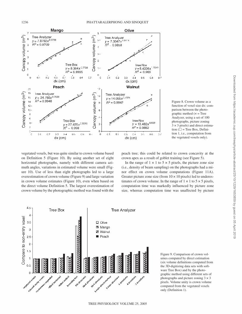
vegetated voxels, but was quite similar to crown volume basedon Definition 5 (Figure 10). By using another set of eighthorizontal photographs, namely with different camera azi-muth angles, variations in estimated volume were small (Fig-ure 10). Use of less than eight photographs led to a largeoverestimation of crown volume (Figure 9) and large variationin crown volume estimates (Figure 10), even when based onthe direct volume Definition 5. The largest overestimation ofcrown volume by the photographic method was found with the

peach tree; this could be related to crown concavity at thecrown apex as a result of goblet training (see Figure 5).

In the range of 1 × 1 to 5 × 5 pixels, the picture zone size(i.e., density of beam sampling) on the photographs had a mi-nor effect on crown volume computations (Figure 11A).Greater picture zone size (from 10 × 10 pixels) led to underes-timates of crown volume. In the range of 1 × 1 to 5 × 5 pixels,computation time was markedly influenced by picture zonesize, whereas computation time was unaffected by picture



Figure 8. Crown volume as afunction of voxel size dx: com-parison between the photo-graphic method (× = TreeAnalyzer, using a set of 100photographs, picture zoning3 × 3 pixels) and direct estima-tion (� = Tree Box, Defini-tion 1, i.e., computation fromthe vegetated voxels only).

Figure 9. Comparison of crown vol-umes computed by direct estimation(six volume definitions computed fromthe 3D-digitizing data sets with soft-ware Tree Box) and by the photo-graphic method using different sets ofphotographs and picture zoning 3 × 3pixels. Volume unity is crown volumecomputed from the vegetated voxelsonly (Definition 1).

Dow



zone size greater than 5 × 5 pixels (Figure 11B). As a result,setting the picture zone size at 3 × 3 pixels provided a good es-timate of crown volume within a reasonable computation time.

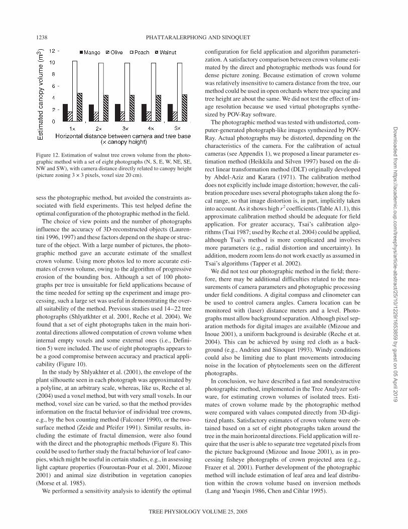
For all trees, the effect of camera distance on crown volumeestimation was small; the distance was in the range of one tofive times canopy height (Figure 12). Compared with esti-mates of crown volume based on the direct volume (Defini-tion 5), estimated crown volume was slightly greater whencamera distance was set equal to canopy height (1% in peachto 11% in walnut) and was minimal when set at two or threetimes canopy height for all trees.

Discussion

In this study, we described and evaluated a photographicmethod to estimate the crown volume of isolated tree canopies.At a given scale, space occupied by the tree canopy has beendefined by parametric shapes (e.g., Norman and Welles 1983,Cescatti 1997) or convex envelopes (Cluzeau et al. 1995).Here we have defined crown volume as the volume of voxelsclassified as canopy space, where voxels were regarded aseither empty (gap fraction = 1) or vegetated (gap fraction < 1),and the transparency information was not used further. Thiskind of binary information is suitable for volume computation;however, it is unsuitable if the aim is to compute vegetationdensity within the voxels.

The first step in the photographic method is to estimate plantsize in order to define a bounding box. The principle is similarto that adopted when using a dendrometric clinometer to deter-mine tree height and crown diameter. Tree size values aver-aged from the set of photographs closely approximated the

value computed from the 3D-digitized data set (Figure 6). Forvolume computation, the bounding box was built from maxi-mum values found for tree height and diameter, thus ensuringthat the whole tree crown was included within the boundingbox. Finally, crown volume was computed from iterative ero-sion of the bounding box, according to plant silhouettes pro-vided by the photographs. This procedure differs from, and issimpler than, other photographic methods. For example,Shlyakhter et al. (2001) computed the intersection of solid an-gles defined by plant silhouettes from camera location, where-as Reche et al. (2004) used a method derived from medicaltomography.

We tested our photographic method quantitatively by com-paring crown volume computed from photographs with crownvolume derived from the 3D-digitizing data set. This may beregarded as a virtual experiment because it allowed us to as-



Figure 10. Comparison between crown volumes computed from the3D-digitizing data sets (Definition 5) and by the photographic meth-od, for different numbers of photographs, using a voxel size of 20 cm.The error bars show the standard deviation of crown volume fromthree different sets of images. The images were synthesized by settinghorizontal camera elevation and camera distance at twice canopyheight. Camera height (1.2–1.5 m) and focal length (7–9 mm) wereset so that the entire canopy was included in the image.

Figure 11. Effect of picture zone size on crown volume (A) and com-putation time (B) for a walnut tree. Volume was computed from a setof 100 photographs, for different voxel sizes. Maximum picture zonesize was defined so that the image of the picture zone on the canopyplane is smaller than voxel size. The computations were done on apersonal computer with CPU Intel Pentium III 1.06 GHz.

Dow



sess the photographic method, but avoided the constraints as-sociated with field experiments. This test helped define theoptimal configuration of the photographic method in the field.

The choice of view points and the number of photographsinfluence the accuracy of 3D-reconstructed objects (Lauren-tini 1996, 1997) and these factors depend on the shape or struc-ture of the object. With a large number of pictures, the photo-graphic method gave an accurate estimate of the smallestcrown volume. Using more photos led to more accurate esti-mates of crown volume, owing to the algorithm of progressiveerosion of the bounding box. Although a set of 100 photo-graphs per tree is unsuitable for field applications because ofthe time needed for setting up the experiment and image pro-cessing, such a large set was useful in demonstrating the over-all suitability of the method. Previous studies used 14–22 treephotographs (Shlyatkhter et al. 2001, Reche et al. 2004). Wefound that a set of eight photographs taken in the main hori-zontal directions allowed computation of crown volume wheninternal empty voxels and some external ones (i.e., Defini-tion 5) were included. The use of eight photographs appears tobe a good compromise between accuracy and practical appli-cability (Figure 10).

In the study by Shlyakhter et al. (2001), the envelope of theplant silhouette seen in each photograph was approximated bya polyline, at an arbitrary scale, whereas, like us, Reche et al.(2004) used a voxel method, but with very small voxels. In ourmethod, voxel size can be varied, so that the method providesinformation on the fractal behavior of individual tree crowns,e.g., by the box counting method (Falconer 1990), or the two-surface method (Zeide and Pfeifer 1991). Similar results, in-cluding the estimate of fractal dimension, were also foundwith the direct and the photographic methods (Figure 8). Thiscould be used to further study the fractal behavior of leaf cano-pies, which might be useful in certain studies, e.g., in assessinglight capture properties (Fouroutan-Pour et al. 2001, Mizoue2001) and animal size distribution in vegetation canopies(Morse et al. 1985).

We performed a sensitivity analysis to identify the optimal

configuration for field application and algorithm parameteri-zation. A satisfactory comparison between crown volume esti-mated by the direct and photographic methods was found fordense picture zoning. Because estimation of crown volumewas relatively insensitive to camera distance from the tree, ourmethod could be used in open orchards where tree spacing andtree height are about the same. We did not test the effect of im-age resolution because we used virtual photographs synthe-sized by POV-Ray software.

The photographic method was tested with undistorted, com-puter-generated photograph-like images synthesized by POV-Ray. Actual photographs may be distorted, depending on thecharacteristics of the camera. For the calibration of actualcameras (see Appendix 1), we proposed a linear parameter es-timation method (Heikkila and Silven 1997) based on the di-rect linear transformation method (DLT) originally developedby Abdel-Aziz and Karara (1971). The calibration methoddoes not explicitly include image distortion; however, the cali-bration procedure uses several photographs taken along the fo-cal range, so that image distortion is, in part, implicitly takeninto account. As it shows high r2 coefficients (Table A1.1), thisapproximate calibration method should be adequate for fieldapplication. For greater accuracy, Tsai’s calibration algo-rithms (Tsai 1987; used by Reche et al. 2004) could be applied,although Tsai’s method is more complicated and involvesmore parameters (e.g., radial distortion and uncertainty). Inaddition, modern zoom lens do not work exactly as assumed inTsai’s algorithms (Tapper et al. 2002).

We did not test our photographic method in the field; there-fore, there may be additional difficulties related to the mea-surements of camera parameters and photographic processingunder field conditions. A digital compass and clinometer canbe used to control camera angles. Camera location can bemonitored with (laser) distance meters and a level. Photo-graphs must allow background separation. Although pixel sep-aration methods for digital images are available (Mizoue andInoue 2001), a uniform background is desirable (Reche et at.2004). This can be achieved by using red cloth as a back-ground (e.g., Andrieu and Sinoquet 1993). Windy conditionscould also be limiting due to plant movements introducingnoise in the location of phytoelements seen on the differentphotographs.

In conclusion, we have described a fast and nondestructivephotographic method, implemented in the Tree Analyzer soft-ware, for estimating crown volumes of isolated trees. Esti-mates of crown volume made by the photographic methodwere compared with values computed directly from 3D-digi-tized plants. Satisfactory estimates of crown volume were ob-tained based on a set of eight photographs taken around thetree in the main horizontal directions. Field application will re-quire that the user is able to separate tree vegetated pixels fromthe picture background (Mizoue and Inoue 2001), as in pro-cessing fisheye photographs of crown projected area (e.g.,Frazer et al. 2001). Further development of the photographicmethod will include estimation of leaf area and leaf distribu-tion within the crown volume based on inversion methods(Lang and Yueqin 1986, Chen and Cihlar 1995).



Figure 12. Estimation of walnut tree crown volume from the photo-graphic method with a set of eight photographs (N, S, E, W, NE, SE,NW and SW), with camera distance directly related to canopy height(picture zoning 3 × 3 pixels, voxel size 20 cm).

Dow



Acknowledgments

The authors are grateful to D. Combes (INRA-Lusignan, France) forthe walnut tree 3D-digitizing data and for assistance in acquiring thepeach tree digitizing data, to P. Kasemsap, S. Thanisawanyangkuraand N. Musigamart (Kasetsart University, Bangkok, Thailand) for as-sistance with acquisition of the mango and olive tree digitizing data,and to the POV-Ray Team who provided POV-Ray freeware and itsdocumentation. Acquisition of the peach tree digitizing data was sup-ported by project “Production Fruitière Intégrée” funded by INRA.Peach trees were made available by CTIFL, Balandran.

References

Abdel-Aziz, Y.I. and H.M. Karara. 1971. Direct linear transformationinto object space coordinates in close range photogrammetry. Proc.Symp. on Close-Range Photogrammetry, Urbana, IL, pp 1–18.

Adam, B., N. Donès and H. Sinoquet. 2002. VegeSTAR: software tocompute light interception and canopy photosynthesis from imagesof 3D digitised plants. Version 3.0. UMR PIAF INRA-UBP,Clermont-Ferrand, France.

Andrieu, B, and H. Sinoquet. 1993. Evaluation of structure descrip-tion requirements for predicting gap fraction of vegetation cano-pies. Agric. For. Meteorol. 65:207–227.

Boudon, F. 2004. Représentation géométrique multi-échelles de l’ar-chitecture des plantes. Ph.D. Thesis, Université Montpellier II,Montpellier, France, 176 p.

Brown, P.L., D. Doley and R.J. Keenan. 2000. Estimating tree crowndimensions using digital analysis of vertical photographs. Agric.For. Meteorol. 100:199–212.

Cescatti, A. 1997. Modelling the radiative transfer in discontinuouscanopies of asymmetric crowns. I. Model structure and algorithms.Ecol. Model. 101:263–274.

Chen, J.M. and J. Cihlar. 1995. Plant canopy gap-size analysis theoryfor improving optical measurements of leaf-area index. Appl. Op-tics 34:6211–6222.

Cluzeau, C., J.L. Dupouey and B. Courbaud. 1995. Polyhedral repre-sentation of crown shape. A geometric tool for growth modelling.Ann. Sci. For. 52:297–306.

den Dulk, J.A. 1989. The interpretation of remote sensing, a feasibil-ity study. Ph.D. Thesis, Wageningen Agricultural Univ., Wagenin-gen, The Netherlands, 173 p.

Falconer, K. 1990. Fractal geometry: mathematical foundation andapplications. John Wiley and Sons, Chichester, UK, 337 p.

Farque, L., H. Sinoquet and F. Colin. 2001. Canopy structure and lightinterception in Quercus petraea seedlings in relation to light re-gime and plant density. Tree Physiol. 21:1257–1267.

Foroutan-Pour, K., P. Dutilleul and D.L. Smith. 2001. Inclusion of thefractal dimension of leafless plant structure in the Beer-Lambertlaw. Agron. J. 93:333–338.

Frazer, G.W., R.A. Fournier, J.A. Trofymow and R.J. Hall. 2001. Acomparison of digital and film fisheye photography for analysis offorest canopy structure and gap light transmission. Agric. For.Meteorol. 109:249–263.

Fuchs, M. and G. Stanhill. 1980. Row structure and foliage geometryas determinants of the interception of light rays in a sorghum rowcanopy. Plant Cell Environ. 3:175–182.

Giuliani, R., E. Magnanini, C. Fragassa and F. Nerozzi. 2000. Groundmonitoring the light–shadow windows of a tree canopy to yieldcanopy light interception and morphological traits. Plant Cell Envi-ron. 23:783–796.

Glassner, A.S. 1989. An introduction to ray tracing. Morgan Kauf-mann Publishers, San Francisco, CA, 119 p.

Heikkila, J. and O. Silven. 1997. A four-step camera calibrationprocedure with implicit image correction. Proc. of the 1997 Con-ference on Computer Vision and Pattern Recognition. IEEEComput. Soc., Washington, DC, pp 1106–1112.

Kimes, D.S. and J.A. Kirchner. 1983. Diurnal variation of vegetationcanopy structure. Int. J. Remote Sens. 4:257–271.

Kutulakos, K.N. and S.M. Seitz. 2000. A theory of shape by spacecarving. Int. J. Comput. Vision 38:199–218.

Lang, A.R.G. 1973. Leaf orientation of a cotton plant. Agric.Meteorol. 11:37–51.

Lang, A.R.G. and X. Yueqin. 1986. Estimation of leaf area index fromtransmission of direct sunlight in discontinuous canopies. Agric.For. Meteorol. 37:229–243.

Laurentini, A. 1996. Surface reconstruction accuracy for active vol-ume intersection. Pattern Recogn. Lett. 17:1285–1292.

Laurentini, A. 1997. How many 2D silhouettes does it take to recon-struct a 3D object? Computer Vision and Image Understanding 67:81–87.

Laurentini, A. 1999. Computing the visual hull of solids of revolution.Pattern Recogn. 32:377–388.

Mizoue, N. 2001. Fractal analysis of tree crown images in relation tocrown transparency. J. For. Plan. 7:79–87.

Mizoue, N. and A. Inoue. 2001. Automatic thresholding of tree crownimages. Jpn. J. For. Plan. 6:75–80.

Morse, R., J. Lawton, M. Dodson and M. Williamson. 1985. Fractaldimension of vegetation and the distribution of arthropod bodylengths. Nature 314:731–732.

Nelson, R. 1997. Modeling forest canopy heights: the effects of can-opy shape. Remote Sens. Environ. 60:327–334.

Nilson, T. 1992. Radiative transfer in nonhomogeneous plant cano-pies. Adv. Bioclimatol. 1:59–88.

Norman, J.M. and J.M. Welles. 1983. Radiative transfer in an array ofcanopies. Agron. J. 75:481–488.

Oker-Blom, P. and S. Kellomaki. 1983. Effect of grouping of foliageon the within-stand and within-crown light regime. Comparisonof random and grouping canopy models. Agric. Meteorol. 28:143–155.

Prusinkiewicz, P. and A. Lindenmayer. 1990. The algorithmic beautyof plants. Springer-Verlag, New York, 228 p.

Reche A., I. Martin and G. Drettakis. 2004. Volumetric reconstructionand interactive rendering of trees from photographs. ACM Trans-actions on Graphics (SIGGRAPH Conference Proceedings) 23:1–10.

Seitz, S.M. and C.R. Dyer. 1997. Photorealistic scene reconstructionby Voxel Coloring. Proc. IEEE CVPR, pp 1067–1073.

Shlyakhter, I., M. Rozenoer, J. Dorsey and S. Teller. 2001. Recon-structing 3D tree model from instrumented photographs. IEEEComput. Graph. Appl. 21:53–61.

Sinoquet, H. and P. Rivet. 1997. Measurement and visualization of thearchitecture of an adult tree based on a three-dimensional digitisingdevice. Trees 11:265–270.

Sinoquet, H., B. Moulia and R. Bonhomme. 1991. Estimating the 3Dgeometry of a maize crop as an input of radiation models: compari-son between 3D digitizing and plant profiles. Agric. For. Meteorol.55:233–249.

Sinoquet, H., S. Thanisawanyangkura, H. Mabrouk and P. Kasemsap.1998. Characterisation of light interception in canopies using 3Ddigitising and image processing. Ann. Bot. 82:203–212.

Sonohat, G., H. Sinoquet, V. Kulandaivelu, D. Combes and F. Les-courret. 2004. Three-dimensional reconstruction of partially 3Ddigitised peach tree canopies. In Proc.: 4th Int. Workshop on Func-tional–Structural Plant Models. Eds. C. Godin, J. Hanan, W. Kurth,A. Lacointe, A. Takenaka, P. Prusinkiewicz, T. DeJong, C. Bever-



Dow



idge and B. Andrieu. UMR AMAP, Montpellier, France, pp 6–8.Takenaka, A., Y. Inui and A. Osawa. 1998. Measurement of three-di-

mensional structure of plants with a simple device and estimationof light capture of individual leaves. Funct. Ecol. 12:159–165.

Tapper, M., P.J. McKerrow and J. Abrantes. 2002. Problems encoun-tered in the implementation of Tsai’s algorithm for camera cal-ibration. Proc. 2002 Australasian Conference on Robotics andAutomation, ARAA, Auckland, pp 66–70.

Tsai, R.Y. 1987. A versatile camera calibration technique for high-ac-curacy 3D machine vision metrology using off-the-self TV cam-eras and lenses. IEEE J. Robotics Autom. 3:323–344.

Zeide, B. and P. Pfeifer. 1991. A method for estimation of fractaldimension of tree crowns. For. Sci. 37:1253–1265.



Appendix 1

Derivation of calibration parameter for digital cameras

In this study, the calibration parameter (k) of the camera isneeded to compute the beam line equation associated witheach pixel of the photograph (see Appendix 2), and to computethe view angle of the virtual camera used in POV-Ray softwareto synthesize photograph-like images. The view angle γc of thephotograph is defined as the angle made by the diagonal of thepicture. It depends on the camera model (i.e., type of lens) andfocal length f (Figure A1.1). The calibration parameter k is thediagonal length of the projected image onto the receptor andhas the same unit as f (usually mm). The receptor is either thefilm in classical cameras or a CCD array (charge-coupled de-vice) in digital cameras. The relationship between γc, f and k is:

tanγ c

2 2

= k

f(A1.1)

Here we propose a method to derive k from a set of picturesof the same object taken at a range of focal lengths. The cam-era is assumed to be a pinhole camera (Figure A1.1) and imagedistortion due to lens properties is neglected.

The object is usually a horizontal line of known length (l)drawn on a vertical plane. The camera is located at the samelevel as the object at a fixed distance D from the vertical plane,where D is chosen so that the line is entirely viewed on the im-age when using maximum zooming (D is about 2–3 m for l =50 cm). From geometrical considerations:

k

f

L

D= (A1.2)

where L is the length of the image diagonal. Note that L and Dcan be expressed in both metric (subscript m) and pixel (sub-script p) units. In Equation A1.2, k is the unknown to be in-ferred, values of f and Lp both change according to zooming,and D is a constant defined by the experimental layout. In digi-tal cameras, the value of f is stored as an image property in theimage file and can be displayed with any imaging software.For each image, the length of the image diagonal in metricunits, Lm, can be computed from the length of the photo-graphed line, both in metric and pixel units, i.e., lm and lp, re-spectively, and the length of image diagonal Lp in pixel units:

L Ll

lm pm

p

=

(A1.3)

In Equation A1.3, lp can be derived from the pixel location(xp, yp) on the x and y axes defining the image plane, whereasLp can be derived from image resolution.

Finally, the calibration parameter k is inferred from Equa-tion A1.2 as the slope of the regression line between variablesDm/Lm and f.

Figure A1.2 shows the regression line for the MinoltaDiMAGE 7i digital camera, and Table A1.1 gives the values ofparameter k for various camera types. The high r 2 coefficientfound in the regression analysis used to derive the calibrationparameter shows that the calibration procedure is valid, eventhough image distortion is neglected (Table A1.1). The valueof k changes markedly with camera type, from 6.5 to 10.9 mmfor the Canon PowerShot A75 and Minolta Dimage 7, respec-tively. In contrast, k values of two cameras of the same type(here Canon PowerShot75 and NikonCoolPix885) show onlysmall variations.

Figure A1.1. Simple camera model(pinhole camera) showing the relation-ship between view angle (γc) of thecamera, focal length ( f ), camera dis-tance (D) and size of the image pro-jected onto the camera receptor (k).

Dow



Appendix 2

Derivation of the beam line equation associated with a pixelon the photograph

Each pixel on the photograph is associated with a beam lineoriginating from the camera location. The line equation de-pends on camera parameters and on pixel location on the im-age. The line equation is needed to compute the list of voxelsassociated with a pixel, i.e., crossed by the beam line. The ori-gin of the system is located at the tree base. The axis X+ pointsto the East, axis Y+ points to the North and axis Z+ points up-ward. The camera is located at C and points to Z+. Imageplane (Pi) is the back projection of the image at a distanceequal to focal length ( f ) perpendicular to camera view direc-tion (Figure A2.1). The equation of the beam line can be writ-ten:

r C u= + λ (A2.1)

where: r is any point (x, y, z) on the beam line; C is camera lo-

cation; and u is a unit vector defining the direction associatedwith each pixel:

u = + + =[ , , ],a b c a b cwith 2 2 2 1 (A2.2)

λ is scalar distance from the beam origin to the point.The beam line equation is defined by vectors C and u, which

are known. For a given image, C is fixed whereas u changesaccording to pixel location in the image.

Computation of camera location (C)

For each photograph, information about camera location andorientation has to be recorded by the operator: camera height(Hc), horizontal distance from tree base (Dc), azimuth (αc), el-evation (βc) and rolling (θc). Then C is derived as:

C = ( cos( ), sin( ), )D D Hc c c c cα α (A2.3)

Calculation of unit vector (u)

We can derive u from the spatial coordinates of two points:P1(x1, y1, z1) and P2(x2, y2, z2):

uP P1 2= − − + − + −

λλwhere = ( ( (1 1 1x x y y z z2

22

22

2) ) )

(A2.4)

Here, P1 is camera location and P2 represents the spatial co-ordinates of a given pixel. To make the calculation simpler, thereference origin is translated to camera location. Thus P1 = (0,0, 0) and Equation A2.4 becomes:

u P2= − + +/ λ λwhere = 22

22

22x y z (A2.5)

Derivation of u reduces to the calculation of P2 for any pixel(xp, yp) as follows: (1) transformation of 2D coordinates (xp, yp)into 3D coordinates (xi, yi, zi); and (2) rotation of the 3D coor-dinates according to camera Euler angles.



Figure A1.2 Relationship between focal length ( f ) and variableDm/Lm for the Minolta DiMAGE 7i digital camera. The calibrationparameter (k = 10.931) is computed as the slope of the regression line.

Table A1.1. Calibration parameter (k) of several camera models.

Camera model Maximum resolution Focal length (mm) View angle (°) k (mm) r2

Canon PowerShot A75 2048 × 1536 5.41–13.4 27.5–62.4 6.5598 0.9976Canon PowerShot A75 2048 × 1536 5.41–13.4 27.4–62.2 6.5295 0.9964Casio QV-3500EX 2544 × 1904 7–21 26.1–66.3 9.3196 0.9851Epson PhotoPC 3100Z 2048 × 1536 7–20.7 24.4–65.2 8.9623 0.9994Fuji FinePix1400Z 1280 × 960 6–18 21.7–59.8 6.903 0.9917Minolta DiMAGE 7i 2560 × 1920 7.2–50.8 12.3–74.4 10.931 0.9983Nikon CoolPix4500 2272 × 1704 7.85–32 16.1–60.0 9.0602 0.9995Nikon CoolPix885 2048 × 1536 8–24 20.9–57.9 8.8532 0.9844Nikon CoolPix885 2048 × 1536 8–24 21.1–58.5 8.9577 0.9894Nikon E995 2048 × 1536 8–32 15.7–57.8 8.8481 0.9998Olympus C-2020Z 1600 × 1200 6.5–19.5 22.6–61.9 7.8036 0.9970Sony DSC-P50 1600 × 1200 6.4–19.2 19.2–53.8 6.4985 0.9995

Dow



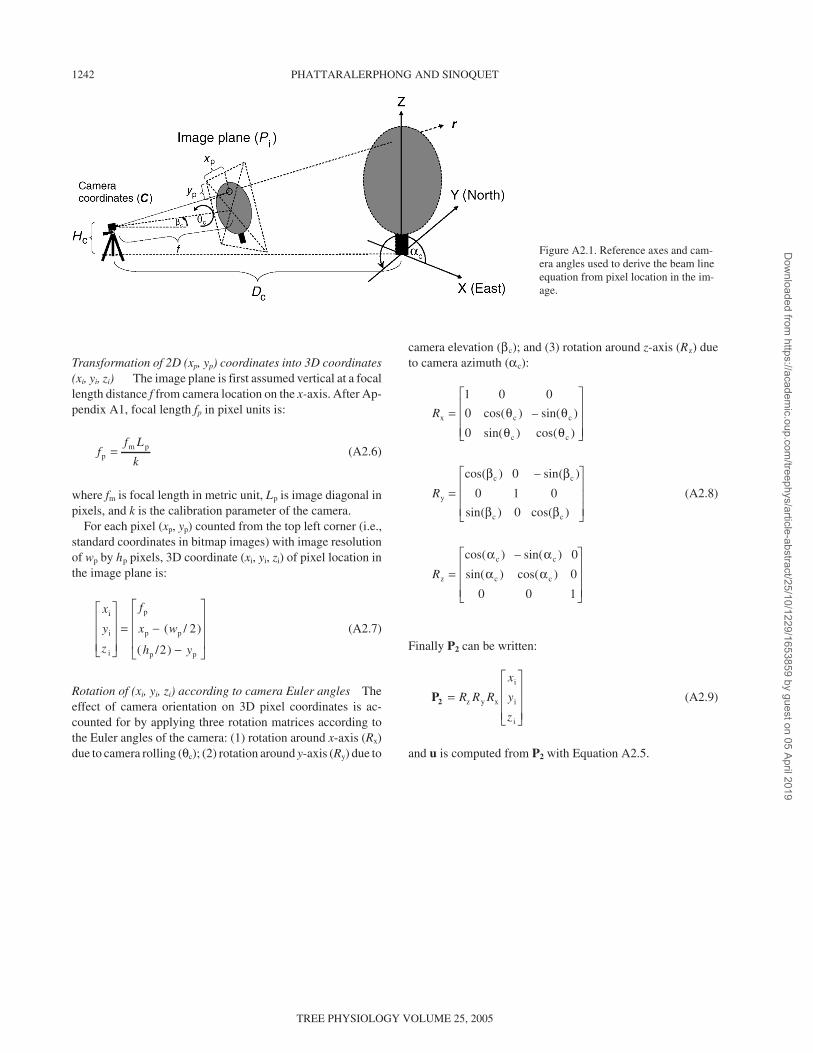
Transformation of 2D (xp, yp) coordinates into 3D coordinates(xi, yi, zi) The image plane is first assumed vertical at a focallength distance f from camera location on the x-axis. After Ap-pendix A1, focal length fp in pixel units is:

ff L

pm p=k

(A2.6)

where fm is focal length in metric unit, Lp is image diagonal inpixels, and k is the calibration parameter of the camera.

For each pixel (xp, yp) counted from the top left corner (i.e.,standard coordinates in bitmap images) with image resolutionof wp by hp pixels, 3D coordinate (xi, yi, zi) of pixel location inthe image plane is:

x

y

z

f

x w

h y

i

i

i

p

p p

p p

= −

−

( / )

( / )

2

2

(A2.7)

Rotation of (xi, yi, zi) according to camera Euler angles Theeffect of camera orientation on 3D pixel coordinates is ac-counted for by applying three rotation matrices according tothe Euler angles of the camera: (1) rotation around x-axis (Rx)due to camera rolling (θc); (2) rotation around y-axis (Ry) due to

camera elevation (βc); and (3) rotation around z-axis (Rz) dueto camera azimuth (αc):

Rx c

1 0 0

0 cos( – sin(= θ θ) c

c c

y

c

)

0 sin( cos(θ θ

β

) )

cos( )

=R

0 – sin

0 1 0

sin

c

c

( )

( )

β

β 0

– sin( 0

sin(

c

z

c c

cos( )

cos( ) )

β

α α

=R α αc c 0

0 0

) cos( )

1

(A2.8)

Finally P2 can be written:

P2 =

R R R

x

y

zz y x

i

i

i

(A2.9)

and u is computed from P2 with Equation A2.5.



Figure A2.1. Reference axes and cam-era angles used to derive the beam lineequation from pixel location in the im-age.

Dow



a method for 3d reconstruction of tree crown - tree physiology

Documents