a methodology for the assessment of the train … · train running safety on bridges pedro aires...
TRANSCRIPT

A METHODOLOGY FOR THE ASSESSMENT OF THE
TRAIN RUNNING SAFETY ON BRIDGES
Pedro Aires Moreira Montenegro e Almeida 2015
A dissertation presented to the Faculty of Engineering of the University of Porto for the degree of Doctor in Civil Engineering.
Supervisor: Professor Rui Calçada
Co-Supervisor : Professor Nelson Vila Pouca


“CONVITE
Defronte da cabana de bambu
respira a esmeralda de um lago.
Virás quando tiveres tempo,
beberemos chá,
na casa de barro coroada de colmo
não encontrarás conforto.
É fácil saber qual é:
frente à porta e antes da cabana de bambu
uma árvore pujante de eternas
afogueadas gemas
anuncia os futuros visitantes.”
(in Oferenda Oriental, Aires Montenegro)


À Alice

THESIS EXAMINING COMMITTEE
The present thesis has been examined on March 12, 2015, at the Faculty of Engineering of
the University of Porto by the following committee:
President:
• Dr. Rui Manuel Carvalho Marques de Faria (by delegation of the Dean of the Faculty of
Engineering of the University of Porto), Full Professor of the Civil Engineering
Department of the Faculty of Engineering of the University of Porto, Porto, Portugal.
Examiners:
• Dr. Makoto Tanabe, Professor of the Department of Mechanical Engineering of the
Faculty of Engineering of the Kanagawa Institute of Technology, Atsugi, Japan.
• Dr. José Maria Goicolea Ruigómez, Full Professor of the Escuela de Ingenieros de
Caminos, Canales y Puertos of the Polytechnic University of Madrid, Madrid, Spain.
• Dr. João Carlos Pombo, Associate Professor in Railway Engineering of the School of
Energy, Geoscience, Infrastructures & Society of the Heriot-Watt University,
Edinburgh, United Kingdom.
• Dr. Raimundo Moreno Delgado, Full Professor (Emeritus) of the Civil Engineering
Department of the Faculty of Engineering of the University of Porto, Porto, Portugal.
• Dr. Rui Artur Bártolo Calçada, Full Professor of the Civil Engineering Department of
the Faculty of Engineering of the University of Porto, Porto, Portugal (Supervisor).


GENERAL CONTENTS
GENERAL CONTENTS ..................................................................................................................... ix
ABSTRACT .................................................................................................................................... xi
RESUMO ...................................................................................................................................... xiii
概要............................................................................................................................................ .xv
LIST OF PUBLICATIONS ............................................................................................................... xvii
ACKNOWLEDGEMENTS/AGRADECIMENTOS ................................................................................ xix
TABLE OF CONTENTS ................................................................................................................. xxiii
LIST OF SYMBOLS ..................................................................................................................... xxxv
CHAPTER 1 - INTRODUCTION ......................................................................................................... 1
CHAPTER 2 - STATE OF THE ART .................................................................................................. 19
CHAPTER 3 - FRAMEWORK OF THE METHODOLOGY FOR THE ASSESSMENT OF THE TRAIN
RUNNING SAFETY ON BRIDGES ................................................................................ 49
CHAPTER 4 - DEVELOPMENT OF A METHOD FOR ANALYZING THE DYNAMIC TRAIN-STRUCTURE
INTERACTION.......................................................................................................... 73
CHAPTER 5 - VALIDATION OF THE TRAIN-STRUCTURE INTERACTION METHOD .......................... 111
CHAPTER 6 - RUNNING SAFETY ANALYSIS OF A HIGH-SPEED TRAIN MOVING ON A VIADUCT UNDER
SEISMIC CONDITIONS ............................................................................................ 149
CHAPTER 7 - CONCLUSIONS AND FUTURE DEVELOPMENTS ........................................................ 211
APPENDIX A - IMPLEMENTATION OF A CONTACT LOOKUP TABLE .............................................. 221
APPENDIX B - COEFFICIENTS FOR THE NORMAL AND TANGENTIAL CONTACT PROBLEMS .......... 229
APPENDIX C - BLOCK FACTORIZATION SOLVER ......................................................................... 233
REFERENCES .............................................................................................................................. 237

xi
ABSTRACT
This thesis focuses on the development of a methodology for the assessment of the train
running safety on bridges. Particular attention is given to the running stability against moderate
and frequent earthquakes which, although may not pose a significant threat to the structural
integrity, can jeopardize the train running safety.
In light of this objective, an overview of recent studies carried out in the field of rail traffic
stability over bridges is presented, along with a review of the different existing methods for
analyzing the dynamic response of the vehicle-structure system.
After going through the most common modeling alternatives, the train-structure interaction
method proposed in this work is presented. Special emphasis is given to the wheel-rail contact
model used to calculate the contact forces that are generated in the contact interface between
the wheel and rail. Most of the existing methods treat the contact forces in the normal and
tangential directions as external forces, whereas the present formulation uses a finite element to
model the behavior in the contact interface, based on the Hertz theory and Kalker's rolling
friction laws. To couple the vehicle and structure, the governing equilibrium equations of both
systems are complemented with additional constraint equations that relate the displacements of
the contact nodes of the vehicle with the corresponding nodal displacements of the structure.
These equations form a single system, with displacements and contact forces as unknowns, that
is solved directly using an optimized block factorization algorithm. The proposed model is
based on the finite element method, which allows the analysis of structures and vehicles with
any degree of complexity. The present formulation is implemented in MATLAB, being the
vehicles and structure modeled with ANSYS.
The implemented vehicle-structure interaction tool is validated with three numerical
applications and with the results obtained in an experimental test. First, the results obtained
with the creep force models implemented in the proposed method are compared with those
obtained with the Kalker's exact theory of rolling contact implemented in the software
CONTACT. In the second application, the tests performed in the Manchester Benchmark are
revisited and replicated with the proposed numerical tool. The third numerical application
consists in the hunting stability analysis of a suspended wheelset. The results obtained with the

Abstract
xii
proposed method for the lateral displacements and yaw rotations of the wheelset are compared
with those obtained with a semi-analytical model described in the literature. In the last
application, an experimental test conducted in the rolling stock test plant of the Railway
Technical Research Institute in Japan, in which a full scale railway vehicle runs over a track
with vertical and lateral deviations is reproduced numerically. The results obtained with the
proposed method are compared with the experimental results and also with the results obtained
using the software DIASTARS.
Finally, a study regarding the running safety of a high-speed train moving over a viaduct
under seismic conditions is conducted using the developed train-structure interaction method.
The studied viaduct is based on an existing flyover type structure of the Portuguese railway
network, while the vehicle consists of a Japanese Shinkansen high-speed train. The seismic
action is represented in terms of artificial accelerograms generated from the elastic spectra
described in EN 1998-1, while the irregularity profiles are generated based on analytical power
spectral density functions. Since no significant nonlinear behavior is likely to be exhibited in
the columns for the levels of seismicity considered in this work, all the analysis are performed
in the elastic domain with a reduction in the stiffness of the columns to account for the concrete
cracking. The running safety analysis of the railway vehicle running over the viaduct is
assessed based on four derailment criteria, being the influence of the seismic intensity level, the
vehicle running speed and the track quality on the running safety evaluated separately. At the
end, all the information obtained in the dynamic analyses is condensed in the so-called running
safety charts, which consist in the global envelope of each analyzed safety criteria as function
of the running speed of the vehicle and the seismic intensity level.

xiii
RESUMO
A presente dissertação centra-se no desenvolvimento de uma metodologia para avaliação da
segurança de circulação de comboios sobre pontes. É dada particular atenção à estabilidade de
circulação na presença de sismos de intensidade moderada que, embora possam não constituir
uma ameaça à integridade estrutural da ponte, podem pôr em causa a segurança de circulação.
À luz deste objetivo, começa-se por apresentar um resumo dos estudos levados a cabo
recentemente no âmbito da segurança de tráfego ferroviário em pontes, conjuntamente com
uma revisão dos diferentes métodos apresentados na bibliografia com vista à análise da
resposta do sistema veículo-estrutura.
Após avaliar-se o atual estado do conhecimento na área, apresenta-se a formulação do
método de interação veículo-estrutura desenvolvido no presente trabalho. É dada uma ênfase
especial ao modelo de contacto roda-carril usado para o cálculo das forças de contacto geradas
na interface de contacto. Na maioria dos métodos existentes, as forças de contacto nas direções
normal e tangencial são tratadas como sendo forças externas, enquanto a presente formulação
utiliza um elemento finito para modelar a interface de contacto, baseado na teoria de Hertz e
nas leis de atrito de rolamento propostas por Kalker. Com vista ao acoplamento do veículo com
a estrutura, as equações de equilíbrio dinâmico são complementadas com equações de
compatibilidade que relacionam os deslocamentos dos nós de contacto do veículo com os
correspondentes deslocamentos nodais da estrutura. Estas equações constituem um sistema
único, cujas incógnitas são deslocamentos e forças de contacto, que pode ser resolvido
diretamente através de um algoritmo de fatorização em blocos. A ferramenta proposta é
baseada no método dos elementos finitos, permitindo assim a análise de veículos e estruturas
com qualquer nível de complexidade. A presente formulação encontra-se implementada em
MATLAB, sendo os veículos e a estrutura modelados com recurso a ANSYS.
A ferramenta de interação veículo-estrutura implementada é validada através de três
aplicações numéricas e de um ensaio experimental. Assim, a primeira aplicação consiste na
comparação dos resultados obtidos pelos modelos de atrito de rolamento implementados no
presente método com os resultados obtidos através da teoria exata de Kalker implementada no
software CONTACT. Na segunda aplicação, os testes realizados no Benchmark de Manchester
Resumo
xiv
são revisitados e replicados com a ferramenta numérica proposta. A terceira aplicação consiste
na análise de estabilidade de um eixo isolado face ao movimento de lacete por ele
experimentado. Os deslocamentos laterais e rotações de lacete obtidos com a ferramenta
desenvolvida são comparados com os resultados obtidos através de um modelo semi-analítico
descrito na bibliografia. Na última aplicação, é reproduzido numericamente um ensaio
experimental realizado na instalação de testes de material circulante do Railway Technical
Research Institute no Japão. Neste teste foi ensaiado um veículo ferroviário à escala real a
circular sobre uma via sujeita a desvios verticais e laterais impostos por atuadores. As respostas
do veículo obtidas com a ferramenta proposta são confrontadas com as respostas experimentais,
bem como com os resultados obtidos no software DIASTARS.
Por último, é realizado um estudo da segurança de circulação de um comboio de
alta-velocidade a circular sobre um viaduto sujeito a ações sísmicas. O viaduto estudado é
baseado numa estrutura do tipo flyover existente na rede ferroviária Portuguesa, enquanto o
veículo consiste num comboio de alta velocidade Japonês. A ação sísmica é representada sob a
forma de acelerogramas artificiais gerados a partir dos espetros elásticos descritos na
EN 1998-1. Já as irregularidades são geradas com base em funções analíticas de densidade
espetral de potência. Uma vez que não é espectável que o comportamento dos pilares atinja um
nível significativo de não-linearidade, todas as análises são realizadas no domínio elástico,
tendo-se tido em conta a redução de rigidez dos pilares devido à fendilhação. A estabilidade de
circulação é analisada com base em quatro critérios de descarrilamento, sendo a influência da
intensidade sísmica, da velocidade do veículo e da qualidade da via na segurança avaliada
separadamente. No final, toda a informação obtida nas análises dinâmicas é condensada em
mapas de segurança de circulação. Estes mapas consistem na envolvente global de cada critério
analisado em função da velocidade de circulação do veículo e da intensidade sísmica.
xv
概要
本論文は,橋梁上を走行する列車の走行安全性の評価手法の高度化を目的としたも
のである.特に,構造物自体の安定性には重大な脅威とはならないものの,上部工に
大きな振動が発生した場合に列車の走行安全性に脅威を及ぼす可能性がある,比較的
小規模かつ頻発する地震に対する走行安全性を対象とした.
この目的のもと,橋梁上の鉄道交通の安定性の分野に関する近年の研究について概
要をまとめ,鉄道車両/構造物システムの動的応答の数値解析に関する既往の手法をレ
ビューした.
最も一般的なモデル化手法の選択肢を経て、本研究で提案された鉄道車両/構造物
の構造連成手法を提示した.車輪/レール間の接触界面に発生する接触力を評価するた
めの,車輪/レール間の接触モデルに特に着目した.既往のほとんどの手法は,接触面
方向,法線方向の接触力を外力として取り扱っているが,提案した定式化の中では,
接触界面を表現するために,Hertzの接触理論と Kalkerの転がり摩擦の法則に基づい
た有限要素を用いた.鉄道車両と構造物の連成を考慮するため,両システムの支配平
衡方程式は,車両側の接触節点の変位と,対応する構造物側の節点変位とを関連付け
る制約式を追加することで補完されている.これらの各システムの方程式は独立して
おり,最適化ブロック分解アルゴリズムを使用して直接得られる未知数である,変位
と接触力を含んでいる.提案手法は有限要素法に基づいていることから,高度に複雑
な構造物,鉄道車両の解析も可能である.提案手法では,ANSYS で鉄道車両や構造
物をモデル化し,MATLAB で実装している.
実装された鉄道車両/構造物の連成解析ツールの妥当性を,三つの数値計算アプリ
ケーションの結果と,一つの実験結果を用いて検証した.第一に,提案手法で実装さ
れているクリープ力モデルにより得られた結果と,ソフトウェア CONTACTに実装さ
れている Kalkerの転がり接触理論を用いて得られたものと比較する.第二に,マンチ
ェスター·ベンチマークで行われたテストを対象に,提案数値解析手法で再現した.第

概要
xvi
三に,取り出した輪軸の蛇行安定解析を対象とした.提案方法を用いて得られた車輪
の横方向変位およびヨー回転角の結果と,文献に記載された半解析モデルを用いて得
られた結果とを比較した.最後に,日本の鉄道総合技術研究所で行われた高速車両走
行試験台の実験試験を数値解析により再現した.車両走行試験は,実物大の鉄道車両
が水平方向および鉛直方向に不整のある軌道上を走行する条件で行われた.提案手法
による結果は,車両走行試験装置の実験結果,およびソフトウェア DIASTARSを用い
て得られた結果と比較した.
最後に,開発した鉄道車両/構造物の解析手法を用いて,高架橋上を高速走行する
鉄道車両の地震時走行安全性に関して検討を行った.対象構造物は,ポルトガルの鉄
道ネットワークに実在する高架道路型高架橋とし,車両は日本の新幹線高速鉄道で使
用されている車両とした.地震作用は,EN-19981に記載されている弾性スペクトルか
ら人工に生成された加速度を用いた.軌道不整形状は,分析パワースペクトル密度関
数に基づいて生成した.本検討で対象とした地震動レベルにおいては,柱に有意な非
線形挙動が現れる可能性が想定されないことから,すべての解析は,コンクリートの
ひび割れを考慮するために柱剛性を低下させた弾性領域で行った.高架橋上を走行す
る鉄道車両の走行安全性に関する四つの脱線基準を,走行安全性に影響を与える地震
動の大きさ,車両の走行速度,軌道の品質に基づいて評価した.最終的に,動的解析
で得られた全結果を基に,列車走行速度と地震動の大きさの関数として,数値解析か
ら得られた安全基準を全て安全側に包絡する,いわゆる走行安全性チャートを作成し
た.

xvii
LIST OF PUBLICATIONS
The following publications have been derived from the development of the present thesis.
International scientific journals
• Neves, S.G.M., Montenegro, P.A., Azevedo, A.F.M., Calçada, R. A direct method for
analyzing the nonlinear vehicle–structure interaction, Engineering Structures, 2014, 69,
pp. 83-89. DOI:10.1016/j.engstruct.2014.02.027.
• Montenegro, P.A., Calçada, R., Vila Pouca, N., Tanabe, M. Running safety assessment
of trains moving over bridges subjected to earthquakes, Earthquake Engineering and
Structural Dynamics, 2015a, (submitted).
• Montenegro, P.A., Neves, S.G.M., Calçada, R., Tanabe, M., Sogabe, M.
Wheel-rail contact formulation for analyzing the lateral train-structure
dynamic interaction, Computers & Structures, 2015, 152, pp. 200-214.
DOI:10.1016/j.compstruc.2015.01.004.
International conference proceedings
• Montenegro, P.A., Calçada, R., Vila Pouca, N. A wheel-rail contact model
pre-processor for train-structure dynamic interaction analysis, In J. Pombo (Ed),
Railways 2012 - 1st International Conference on Railway Technology: Research,
Development and Maintenance, Las Palmas de Gran Canaria, Spain, 2012.
• Montenegro, P.A., Neves, S.G.M., Azevedo, A.F.M., Calçada, R. "A nonlinear
vehicle-structure interaction methodology with wheel-rail detachment and
reattachment", In M. Papadrakakis, N.D.Lagaros, V. Plevris (Ed), COMPDYN 2013 -
4th ECCOMAS Thematic Conference on Computational Methods in Structural
Dynamics and Earthquake Engineering, Kos, Greece, 2013.

List of publications
xviii
• Montenegro, P.A., Neves, S.G.M., Calçada, R., Tanabe, M., Sogabe, M. "A three
dimensional train-structure interaction methodology: Experimental validation", In J.
Pombo (Ed), Railways 2014 - 2nd International Conference on Railway Technology:
Research, Development and Maintenance, Ajaccio, Corsica, France, 2014.
• Neves, S.G.M., Montenegro, P.A., Azevedo, A.F.M., Calçada, R. "A direct method for
analysing the nonlinear vehicle-structure interaction in high-speed railway lines", In J.
Pombo (Ed), Railways 2014 - 2nd International Conference on Railway Technology:
Research, Development and Maintenance, Ajaccio, Corsica, France, 2014.
• Montenegro, P.A., Neves, S.G.M., Calçada, R., Tanabe, M., Sogabe, M. "A nonlinear
vehicle-structure interaction methodology for the assessment of the train running
safety", In A. Cunha, E. Caetano, P. Ribeiro, G. Müller (Ed), EURODYN 2014 - 9th
International Conference on Structural Dynamics, Porto, Portugal, 2014.
• Montenegro, P.A., Calçada, R., Vila Pouca, N. "Dynamic stability of trains moving over
bridges subjected to seismic excitations", In P. Iványi and B.H.V. Topping (Ed), ECT
2014 - 9th International Conference on Engineering Computational Technology,
Naples, Italy, 2014.
National conference proceedings
• Montenegro, P.A., Calçada, R., Vila Pouca, N. "A vehicle-structure interaction method
for analyzing the train running safety", In A. Filho, J. Sousa and R. Pinto (Ed),
IBRACON 2014 - 56th Brazilian Conference on Concrete - 4th Symposium on Railway
and Road Infrastructure, Natal, Brazil, 2014
• Montenegro, P.A., Calçada, R., Vila Pouca, N. "Avaliação da segurança de circulação
de um comboio de alta-velocidade sobre um viaduto em condições sísmicas", In J.M.
Catarino, J. Almeida Fernandes, M. Pipa and J. Azevedo (Ed), JPEE 2014 - 5as
Jornadas Portuguesas de Engenharia de Estruturas, Lisbon, Portugal, 2014.

xix
ACKNOWLEDGMENTS / AGRADECIMENTOS
It has been a long journey, longer than expected, filled with both exciting moments and
frustrating days. However, in the end, the feeling of accomplishment, the personal and
professional experience earned and the new friendships established, compensate most of the
drawbacks experienced during this last five years. Therefore, I want to express my sincere
gratitude to all who have accompanied me during my PhD that, through their friendship and
understanding, contributed to the achievement of this thesis. In particular, I would like to thank:
• My supervisor, Prof. Rui Calçada, for his unconditional support and encouragement
throughout my research work. The encouraging words given in the most difficult times
were, in most cases, as important as the useful scientific discussions that took place
during these last five years. Therefore, I want to thank him not only for the knowledge
acquired during this journey, but also for the friendship established between us.
• My co-supervisor, Prof. Nelson Vila Pouca, for the pleasant and informal stance that he
showed during our discussions. His contribution for a better understanding of topics
regarding earthquake engineering was of the utmost importance for the development of
this work. Our friendship that started almost ten years ago, still during my graduation,
will always be kept in the future.
• Prof. Makoto Tanabe for granting me the opportunity of doing an internship in Japan in
the Kanagawa Institute of Technology and in the Railway Technical Research Institute
(RTRI). I wish to thank him for the warm welcome in his institution and for his
unconditional scientific and personal support during my stay in Japan. I'll always
remember the help he provided during my time in Tokyo in terms of scientific advice,
bureaucratic issues, language barriers and cultural adaptation. Finally, I also wish to
thank him for all the paperwork provided to apply for the Japanese student visa.
• Dr. Masamichi Sogabe for being my supervisor during my internship in the RTRI. I
wish to express my gratitude for the valuable scientific advices given during my stay, as
well as the experimental data provided for the validation of the models developed in this
Acknowledgments/Agradecimentos
xx
work. I also want to thank him for his friendship demonstrated both during work and
during more relaxed times.
• Fundação para a Ciência e Tecnologia for the financial support provided under the PhD
grant SFRH/BD/48320/2008.
• REFER for the data provided regarding the Alverca railway viaduct.
• My friend and engineer Sérgio Neves for all his friendship and scientific support given
during the implementation of the train-structure interaction method developed in this
work. Moreover, I wish to thank him for the knowledge he provided me in terms of
programming, especially in MATLAB.
• Prof. Rui Faria, from the Faculdade de Engenharia da Universidade do Porto, for the
helpful discussions regarding the nonlinear formulation of the contact model.
• Prof. Jose Maria Goicolea, from the Universidad Politécnica de Madrid (UPM), for his
valuable scientific advices, especially regarding the lateral dynamics of the
train-structure system. I wish to express my gratitude for his availability to exchange
some impressions that introduce me to the topic of this work.
• Dr. Pablo Antolín, from the UPM, for his helpful advices regarding the train-structure
dynamics and for all the literature provided in the beginning of this work.
• Dr. Edwin Vollebregt, from the Technische Universiteit Delft and VORtech Computing,
for helping me on validating the creep models implemented in this work.
• Prof. Simon Iwnicki and Dr. Philip Shackleton, from the Institute of Railway Research
in Huddersfield, for the data provided from the Manchester Benchmark to validate the
wheel-rail contact model implemented in this work.
• Prof. João Pombo, from the Heriot Watt University, for our valuable discussions
regarding the wheel-rail contact models and for the literature provided during this work.
• All the members of the Structural Mechanics Lab of the RTRI where I spent two
months during my internship, namely Dr. Humiaki Uehan, Munemasa Tokunaga,
Tsutomu Watanabe, Shintaro Minoura, Matsuoka Kodai, Hidenori Takagi and
Ms. Sawako Murai. I wish to thank them for the warm welcome and for the nice
welcome and farewell dinners presented to me. Moreover, I will always remember the
wonderful coffee given by Ms. Murai everyday at 10:30 and 15:30 sharp.

Acknowledgments/Agradecimentos
xxi
• My friend and engineer Munemasa Tokunaga, for being my mentor of the Japanese
culture, for helping me during my stay in Japan and, more recently, for translating the
abstract of this thesis to Japanese language.
• Dr. Hajime Wakui and Dr. Nobuyuki Matsumoto, from the RTRI, for their valuable
scientific advices during my stay in Tokyo.
• Ms. Yoko Taniguchi, from the International Affairs Division of the RTRI, for helping
me in the bureaucratic issues regarding my internship.
• All colleagues from the railways research group of my faculty, namely, Alejandro de
Miguel, Andreia Meixedo, Carlos Albuquerque, Cristiana Bonifácio, Cristina Ribeiro,
Diogo Ribeiro, Joana Delgado, João Barbosa, João Francisco, João Rocha, Joel
Malveiro, Nuno Santos, Nuno Ribeiro, Pedro Jorge and Sérgio Neves.
• All other friends from my faculty, in particular, André Monteiro, Despoina Skoulidou,
Diogo Oliveira, Jiang Yadong, Luís Macedo, Luís Martins, Mário Marques, Miguel
Araújo, Miriam López, Nuno Pereira and Rui Barros.
• My closest friends, Artur Santos, Francisco Cruz, João Rosas, Jorge Veludo, Nuno
Guerra, Pedro Baltazar and Rui Conceição.
• À minha família mais chegada, em particular à Avó Fininha, Babá, Chico, Golias,
Madrinha Elisa, Madrinha São, Manel Zé, Manuel João, Milu, Tia Graça, Tio Miguel e
Sebastião, por todo o apoio dado ao longo desta jornada.
• Aos meus pais, Papá e Mamã, irmãos, Joana e João, cunhado, Fábio, e sobrinhos, Alice
e Henrique, por me terem ouvido e compreendido nos momentos mais difíceis deste
trabalho. Peço desculpas por alguns momentos de menor paciência da minha parte que
foram ocorrendo ao longo destes últimos cinco anos, em especial no primeiro ano,
quando tudo parecia impossível.
• À Erica, por ter sido um dos grandes pilares ao longo destes últimos anos nos quais
desenvolvi este trabalho. A ela devo grande parte desta conquista porque, apesar de não
ter colaborado de uma forma direta no desenvolvimento dos trabalhos, soube-me
sempre apoiar nos momentos em que pensei desistir, nos momentos em que estive fora e
em todos os outros momentos em que, por causa do trabalho, não pude estar presente.
Agradeço ainda o facto de me ter ajudado a treinar as apresentações que fui fazendo ao

Acknowledgments/Agradecimentos
xxii
longo deste período, ao ponto de decorar termos como "contact point", "wheel-rail
contact" e "train running safety".
• Por fim, mas nem por isso menos importante, gostaria de agradecer à minha sobrinha
Alice que, no último ano e meio, percorreu um caminho que nunca ninguém quis
imaginar que uma menina como ela tivesse que percorrer. Eu precisei de 29 anos para
arranjar coragem para percorrer recentemente os 21 km de uma meia-maratona...e
precisarei ainda de pelo menos mais um ano para conseguir atingir os 42 km. No
entanto, a Alice, com apenas 4 anos, já percorreu dezenas de maratonas e em todas elas
não só chegou ao fim, como também as venceu, sem se queixar uma única vez de todo o
esforço despendido. Por tudo isto e mais alguma coisa, a ela dedico esta tese.
January 6, 2015
xxiii
TABLE OF CONTENTS
Chapter 1 - Introduction ..................................................................................................... 1
1.1 SCOPE OF THE THESIS ........................................................................................................... 1
1.2 MOTIVATION AND OBJECTIVES ............................................................................................. 4
1.3 STRUCTURE OF THE THESIS ................................................................................................... 6
Chapter 2 - State of the art ................................................................................................. 9
2.1 INTRODUCTION ..................................................................................................................... 9
2.2 PAST STUDIES CONCERNING THE ASSESSMENT OF THE TRAIN RUNNING SAFETY ON
BRIDGE ............................................................................................................................... 10
2.3 METHODS FOR ANALYZING THE DYNAMIC BEHAVIOR OF THE STRUCTURE AND VEHICLE .... 17
2.3.1 Moving loads model .................................................................................................. 17
2.3.2 Virtual path method ................................................................................................... 18
2.3.3 Vehicle-structure interaction methods ....................................................................... 19
2.3.3.1 Iterative method .............................................................................................. 19
2.3.3.2 Condensation method ..................................................................................... 22
2.3.3.3 Direct method ................................................................................................. 23
2.3.3.4 Methods considering the wheel and rail geometries ...................................... 25
2.4 WHEEL-RAIL CONTACT MODELS ......................................................................................... 26
2.4.1 Geometric contact problem ........................................................................................ 27

Table of contents
xxiv
2.4.1.1 Offline contact search ..................................................................................... 27
2.4.1.2 Online contact search ...................................................................................... 28
2.4.2 Normal contact problem............................................................................................. 29
2.4.3 Tangential contact problem ........................................................................................ 31
2.5 NORMS AND RECOMMENDATIONS CONCERNING THE SAFETY OF RAILWAY TRAFFIC ........... 32
2.5.1 Introduction ................................................................................................................ 32
2.5.2 European standards .................................................................................................... 33
2.5.2.1 Criteria regarding the bridge deformation control .......................................... 33
2.5.2.1.1 Vertical deflection of the deck ............................................................ 33
2.5.2.1.2 Transverse deflection of the deck ....................................................... 34
2.5.2.1.3 Deck twist ........................................................................................... 34
2.5.2.1.4 Vertical displacement of the upper surface at the end of the deck ..... 35
2.5.2.1.5 Longitudinal displacement of the upper surface at the end of the
deck ..................................................................................................... 36
2.5.2.2 Criteria regarding the bridge vibration control ............................................... 36
2.5.2.2.1 Vertical acceleration of the deck......................................................... 36
2.5.2.2.2 Lateral vibration of the deck ............................................................... 37
2.5.2.3 Criteria regarding the control of the wheel-rail contact forces ....................... 37
2.5.2.3.1 Maximum dynamic vertical wheel load .............................................. 37
2.5.2.3.2 Maximum total dynamic lateral contact force applied by a
wheelset .............................................................................................. 37
2.5.2.3.3 Ratio of the lateral to the vertical contact forces of a wheel ............... 37
2.5.2.3.4 Wheel unloading ................................................................................. 38
2.5.3 Japanese standards ..................................................................................................... 38
2.5.3.1 Verification of safety ...................................................................................... 39

Table of contents
xxv
2.5.3.1.1 Running safety in ordinary conditions ................................................ 39
2.5.3.1.2 Displacements associated with the running safety in seismic
conditions ............................................................................................ 41
2.5.3.2 Verification of restorability ............................................................................ 42
2.5.3.2.1 Restorability of track damage in ordinary conditions ......................... 42
2.5.3.2.2 Restorability of track damage in seismic conditions .......................... 43
2.5.4 North American standards ......................................................................................... 43
2.5.4.1 Verification of derailment .............................................................................. 44
2.5.4.1.1 Requirements to steady state curving ................................................. 44
2.5.4.1.2 Requirements for transition curves ..................................................... 45
2.5.4.1.3 Requirements for dynamic curving .................................................... 45
2.5.4.1.4 Response to elevation irregularity ...................................................... 45
2.5.4.1.5 Response to cross level irregularity .................................................... 46
2.5.4.1.6 Response to alignment irregularity ..................................................... 46
2.5.4.2 Verification of dynamic stability .................................................................... 47
Chapter 3 - Framework of the methodology for the assessment of the train
running safety on bridges ........................................................................ 49
3.1 INTRODUCTION ................................................................................................................... 49
3.2 OVERVIEW OF THE METHODOLOGY FOR THE ASSESSMENT OF THE TRAIN RUNNING SAFETY
ON BRIDGES ........................................................................................................................ 50
3.2.1 Background ................................................................................................................ 50
3.2.2 Description of the methodology................................................................................. 51
3.3 SOURCES OF EXCITATION OF THE TRAIN-STRUCTURE SYSTEM ............................................ 52
3.3.1 Seismic action ............................................................................................................ 52

Table of contents
xxvi
3.3.1.1 Representation of the seismic action .............................................................. 52
3.3.1.2 Generation of artificial accelerograms............................................................ 53
3.3.2 Track irregularities ..................................................................................................... 54
3.3.2.1 Types of track irregularities ............................................................................ 54
3.3.2.2 Power spectral density functions .................................................................... 55
3.3.2.3 Generation of irregularity profiles .................................................................. 57
3.3.3 Other sources of excitation ........................................................................................ 58
3.4 MODELING OF THE SEISMIC BEHAVIOR OF THE BRIDGE PIERS .............................................. 58
3.4.1 Introduction ................................................................................................................ 58
3.4.2 Monotonic response of the bridge piers ..................................................................... 58
3.4.3 Nonlinear dynamic analysis ....................................................................................... 59
3.4.4 Calibration of the effective stiffness of the bridge piers ............................................ 61
3.5 DERAILMENT MECHANISMS AND SAFETY CRITERIA ............................................................ 61
3.5.1 Wheel flange climbing ............................................................................................... 62
3.5.1.1 Derailment mechanism ................................................................................... 62
3.5.1.2 Nadal criterion ................................................................................................ 63
3.5.1.3 Weinstock criterion ......................................................................................... 64
3.5.1.4 Modified Nadal criterion based on the lateral impact duration ...................... 65
3.5.2 Track panel shift......................................................................................................... 66
3.5.2.1 Derailment mechanism ................................................................................... 66
3.5.2.2 Prud'homme criterion ..................................................................................... 67
3.5.3 Gauge widening caused by rail rollover .................................................................... 67
3.5.3.1 Derailment mechanism ................................................................................... 67
Table of contents
xxvii
3.5.3.2 Rail roll criterion ............................................................................................ 68
3.5.4 Wheel unloading ........................................................................................................ 69
3.5.5 Summary of the running safety criteria ..................................................................... 70
3.6 CONCLUDING REMARKS ..................................................................................................... 70
Chapter 4 - Developement of a method for analyzing the dynamic
train-structure interaction ................................................................. 73
4.1 INTRODUCTION ................................................................................................................... 73
4.2 WHEEL-RAIL CONTACT FINITE ELEMENT ............................................................................ 74
4.2.1 Description of the element ......................................................................................... 74
4.2.2 Coordinate system of the element .............................................................................. 75
4.3 GEOMETRIC CONTACT PROBLEM......................................................................................... 77
4.3.1 Parameterization of the rail and wheel profiles ......................................................... 77
4.3.1.1 Coordinate systems of the rail and wheel profiles .......................................... 78
4.3.1.2 Parameterization of the rail profile ................................................................. 78
4.3.1.3 Parameterization of the wheel profile ............................................................. 80
4.3.2 Contact point search ................................................................................................... 81
4.3.2.1 Convex contact search .................................................................................... 82
4.3.2.2 Concave contact search .................................................................................. 85
4.4 NORMAL CONTACT PROBLEM ............................................................................................. 87
4.4.1 Hertz contact theory ................................................................................................... 87
4.4.2 Geometry of the surfaces in contact........................................................................... 88
4.4.3 Normal contact pressure ............................................................................................ 90
Table of contents
xxviii
4.5 TANGENTIAL CONTACT PROBLEM ....................................................................................... 92
4.5.1 Creep phenomenon .................................................................................................... 92
4.5.2 Basic equations of the rolling contact ........................................................................ 93
4.5.3 Creep force theories ................................................................................................... 95
4.5.3.1 Kalker's linear theory ...................................................................................... 95
4.5.3.2 Polach method ................................................................................................ 97
4.5.3.3 Kalker's book of tables ................................................................................... 98
4.6 FORMULATION OF THE TRAIN-STRUCTURE COUPLING SYSTEM .......................................... 100
4.6.1 Governing equations of motion ................................................................................ 100
4.6.1.1 Force equilibrium.......................................................................................... 100
4.6.1.2 Incremental formulation for nonlinear analysis ............................................ 102
4.6.1.3 Updating of the effective stiffness matrix .................................................... 104
4.6.2 Contact constraint equations .................................................................................... 104
4.6.3 Complete system of equations ................................................................................. 105
4.6.4 Algorithm for solving the train-structure interaction problem ................................. 106
4.7 CONCLUDING REMARKS .................................................................................................... 108
Chapter 5 -Validation of the train-structure interaction method .................... 111
5.1 INTRODUCTION ................................................................................................................. 111
5.2 VALIDATION OF THE IMPLEMENTED CREEP FORCE MODELS .............................................. 112
5.2.1 Description of the analyzed cases ............................................................................ 112
5.2.2 Comparison between the creep force models .......................................................... 113

Table of contents
xxix
5.3 THE MANCHESTER BENCHMARK ...................................................................................... 118
5.3.1 Description of the benchmark .................................................................................. 118
5.3.2 Analysis results ........................................................................................................ 119
5.3.2.1 Contact point positions ................................................................................. 120
5.3.2.2 Rolling radius difference .............................................................................. 121
5.3.2.3 Contact angles .............................................................................................. 122
5.3.2.4 Longitudinal creepages ................................................................................. 123
5.3.2.5 Lateral creepages .......................................................................................... 124
5.3.2.6 Spin creepages .............................................................................................. 125
5.3.2.7 Conclusions .................................................................................................. 126
5.4 HUNTING STABILITY ANALYSIS OF A SUSPENDED WHEELSET ............................................ 127
5.4.1 The hunting phenomenon ........................................................................................ 127
5.4.2 Numerical model ...................................................................................................... 128
5.4.3 Governing equations of motion of the semi-analytical model ................................. 129
5.4.4 Analysis results ........................................................................................................ 131
5.5 SIMULATION OF AN EXPERIMENTAL TEST CONDUCTED IN A ROLLING STOCK TEST PLANT. 134
5.5.1 Background and description of the experimental test .............................................. 134
5.5.2 Numerical model ...................................................................................................... 136
5.5.2.1 Structure model ............................................................................................ 136
5.5.2.2 Vehicle model ............................................................................................... 136
5.5.3 Analysis results ........................................................................................................ 139
5.6 CONCLUDING REMARKS ................................................................................................... 147

Table of contents
xxx
Chapter 6 - Running safety analysis of a high-speed train moving on a
viaduct under seismic conditions ....................................................... 149
6.1 INTRODUCTION ................................................................................................................. 149
6.2 NUMERICAL MODEL OF THE VIADUCT ............................................................................... 150
6.2.1 Description of the Alverca railway viaduct ............................................................. 150
6.2.2 Finite element model of the idealized viaduct ......................................................... 152
6.2.3 Dynamic properties of the viaduct ........................................................................... 155
6.3 DEFINITION OF THE SEISMIC ACTION ................................................................................. 156
6.3.1 Artificial accelerograms ........................................................................................... 156
6.3.2 Time offset between the beginning of the earthquake and the entry of the vehicle in
the viaduct ................................................................................................................ 159
6.4 MODELING OF THE SEISMIC BEHAVIOR OF THE PIERS ........................................................ 160
6.4.1 Monotonic response of the piers .............................................................................. 160
6.4.2 Nonlinear dynamic analysis ..................................................................................... 162
6.4.3 Calibration of the effective stiffness of the piers ..................................................... 164
6.4.4 Dynamic properties of the viaduct considering the effective stiffness of the piers . 166
6.5 NUMERICAL MODEL OF THE VEHICLE ................................................................................ 167
6.5.1 Description of the Shinkansen high-speed train ...................................................... 167
6.5.2 Finite element model of the vehicle ......................................................................... 167
6.5.3 Dynamic properties of the vehicle ........................................................................... 169
6.6 DEFINITION OF THE TRACK IRREGULARITIES ..................................................................... 170
Table of contents
xxxi
6.6.1 Main characteristic of the generated irregularity profiles ........................................ 170
6.6.2 Generated irregularity profiles ................................................................................. 170
6.7 DYNAMIC BEHAVIOR OF THE TRAIN-STRUCTURE SYSTEM ................................................. 173
6.7.1 Introduction .............................................................................................................. 173
6.7.2 Dynamic response of the viaduct ............................................................................. 173
6.7.2.1 Vertical response .......................................................................................... 174
6.7.2.2 Lateral response ............................................................................................ 175
6.7.2.3 Influence of the effective stiffness of the piers............................................. 177
6.7.3 Dynamic response of the vehicle ............................................................................. 178
6.7.3.1 Vertical response .......................................................................................... 178
6.7.3.2 Lateral response ............................................................................................ 180
6.7.3.3 Influence of the suspension stoppers ............................................................ 184
6.7.3.4 Influence of the time offset between the beginning of the earthquake and the
entry of the vehicle in the viaduct ................................................................ 186
6.8 RUNNING SAFETY ANALYSIS ............................................................................................. 189
6.8.1 Introduction .............................................................................................................. 189
6.8.2 Influence of the seismic intensity level .................................................................... 190
6.8.3 Influence of the train running speed ........................................................................ 195
6.8.4 Influence of the track quality ................................................................................... 200
6.8.5 Running safety charts ............................................................................................... 203
6.8.6 Critical analysis of the running safety criteria ......................................................... 204
6.8.6.1 Nadal criterion evaluation ............................................................................ 204
6.8.6.2 Wheel unloading criterion evaluation .......................................................... 206

Table of contents
xxxii
6.8.6.3 Evaluation of the remaining criteria ............................................................. 207
6.9 CONCLUDING REMARKS .................................................................................................... 207
Chapter 7 - Conclusions and future developments ................................................ 211
7.1 CONCLUSIONS .................................................................................................................. 211
7.2 FUTURE DEVELOPMENTS .................................................................................................. 217
Appendix A - Implementation of a contact lookup table ..................................... 221
A.1 INTRODUCTION ................................................................................................................. 221
A.2 COORDINATE SYSTEMS ..................................................................................................... 221
A.3 PARAMETERIZATION OF THE RAIL AND WHEEL PROFILES .................................................. 222
A.3.1 Parameterization of the rail profile .......................................................................... 222
A.3.2 Parameterization of the wheel profile ...................................................................... 223
A.4 CONTACT POINT SEARCH AND TABLE STORAGE ................................................................ 225
Appendix B - Coefficients for the normal and tangential contact
problems ............................................................................................ 229
B.1 INTRODUCTION ................................................................................................................. 229
B.2 HERTZ COEFFICIENTS FOR COMPUTING THE SEMI-AXES OF THE CONTACT ELLIPSE ........... 229
B.3 HERTZ CONSTANT FOR COMPUTING THE GENERALIZED STIFFNESS .................................... 230
B.4 KALKER'S CREEPAGE COEFFICIENTS ................................................................................. 231

Table of contents
xxxiii
Appendix C - Block factorization solver .................................................................... 233
C.1 INTRODUCTION ................................................................................................................. 233
C.2 SOLVER FORMULATION .................................................................................................... 233
References.. ........................................................................................................................... 237

xxxv
LIST OF SYMBOLS
For clarity purposes, all the abbreviations, notations and symbols presented in this list are
defined in the text when first used. Generally, the use of the same symbol for different entities
is avoided. However, in situations in which such procedure proved to be inadequate, the risk of
misunderstanding is minimized by preventing the simultaneous use of the same symbol for
different entities in the same context. The list is ordered alphabetically.
ABBREVIATIONS
2D / 3D Two-dimensional / Three-dimensional
AAR Association of American Railroads
BS Bending Shape deflection
CWC Characteristic Wind Curve
DOF Degree of Freedom
EN European Norm
GPU Graphic Processing Unit
HSLM High Speed Load Model
JIS Japanese Industrial Standards
NA National Annex
PGA Peak Ground Acceleration
PSD Power Spectral Density
RTRI Railway Technical Research Institute
SI Spectral Index
TS Translation Shape deflection
TSI Technical Specifications for Interoperability
UIC International Union of Railways

List of symbols
xxxvi
NOTATIONS
( )⋅d Elemental variation of ( )⋅
( )⋅∆ Increment or variation of ( )⋅
( )⋅⋅ First time derivative of ( )⋅
( )⋅⋅⋅ Second time derivative of ( )⋅
( )⋅ Modulus of ( )⋅
( )⋅ Norm of ( )⋅
( ) ( )⋅⋅ Scalar product between ( )⋅ and ( ) .
( ) ( )×⋅ Cross product between ( )⋅ and ( ) .
( )0⋅ Referred to the initial value
( )A⋅ Referred to the alignment irregularity
( )b⋅ Referred to the base shear
( )bg⋅ Referred to the bogie
( )C⋅ Referred to the cross level irregularity
( )ce⋅ Referred to the contact element
( )c⋅ Referred to the contact point coordinate system
( )cb⋅ Referred to the carbody
( )cr⋅ Referred to cracking
( )dyn⋅ Referred to dynamic
( )eff⋅ Referred to effective
( )ela⋅ Referred to elastic
( )ext⋅ Referred to the external loads
( )F⋅ Referred to the free nodal degrees of freedom
( )G⋅ Referred to the gauge irregularity
( )g⋅ Referred to the global coordinate system
( ) IV⋅ Referred to the intersection volume

List of symbols
xxxvii
( )I⋅ Referred to the free nodal degrees of freedom belonging to linear elements
( )i⋅ Referred to the iteration i
( ) ( ) lftlft ⋅⋅ Referred to the left side
( ) lim⋅ Referred to the limit value of ( )⋅
( )max⋅ Referred to the maximum
( )n⋅ Referred to the nth quantity / Referred to the normal contact force
( )O⋅ Referred to the origin of a coordinate system
( )P⋅ Referred to the prescribed degrees of freedom
( )R⋅ Referred to the free nodal degrees of freedom belonging to nonlinear elements
( ) ( )rhtrht ⋅⋅ Referred to the right side
( )r⋅ Referred to the rail / Referred to the rail profile coordinate system
( )S⋅ Referred to the structure
( )sta⋅ Referred to static
( )T⋅ Referred to the transpose of ( )⋅
( )t⋅ Referred to the time step t
( )te⋅ Referred to the target element
( )t⋅ Referred to the target element coordinate system
( )tc⋅ Referred to the track centerline coordinate system
( )V⋅ Referred to the vehicle / Referred to the elevation irregularity
( )w⋅ Referred to the wheel / Referred to the wheel profile coordinate system
( )ws⋅ Referred to the wheelset / Referred to the wheelset coordinate system
( ) tw,⋅ Referred to the wheel tread
( ) fw,⋅ Referred to the wheel flange
( ) zyx ,,⋅ Referred to the x, y or z axis
( )Y⋅ Referred to the degrees of freedom belonging of the internal nodes added by the contact element
( )η⋅ Referred to the lateral creepage / creep force

List of symbols
xxxviii
( )ξ⋅ Referred to the longitudinal creepage / creep force
( )φ⋅ Referred to the spin creepage / spin creep moment
SCALARS
Latin symbols
A Amplitude / Irregularity scale factor / Hertz geometric parameter
aaa ɺɺɺ,, Displacement, velocity and acceleration
gaɺɺ Ground motion acceleration
a, b Semi-axes of the contact ellipse
B Hertz geometric parameter
Ch Hertz constant
d Penetration between the two contacting bodies
E Young modulus
F Force
f Frequency
f (s) Surface defining function
G Shear modulus
h Vertical distance
I Intensity function
i, j Indices
Kh Hertz generalized stiffness coefficient
L Span length
l Half of the gauge
M Moment
m, n Hertz coefficients
Q Vertical contact force

List of symbols
xxxix
R Radius of curvature
R0 Initial rolling radius of the wheel
Rr Correlation function
r Irregularity
rɺ Rigid body slip at the contact area
S Power spectral density function
s Surface parameter
sɺ Actual slip at the contac area
T Structural period / Return period of the seismic action
t Time / Deck twist
V Vehicle speed
v Relative tangential elastic displacement at the contact area
x, y, z Cartesian coordinate in a 3D coordinate system
Y Lateral contact force
Greek symbols
α Parameter of the α method
β Newmark integration parameter
Γ Contact area
γ Contact angle / Newmark integration parameter
δ Deflection / Displacement
ε Tolerance / Gradient of tangential stress
URPWN ,,,,ζ Safety criteria factors (Nadal, Weinstock, Prud'homme, rail rollover and wheel unloading)
θ Hertz angular parameter
tθ Angular rotation between decks
κ Surface curvature

List of symbols
xl
λ Wavelength
µ Friction coefficient
ν Poisson's ratio
σ Normal stress
τ Tangential stress
υ Creepage
φ Roll angle or rotation / Phase angle
ψ Yaw angle or rotation
Ω Spatial frequency
ω Angular frequency
VECTORS AND MATRICES
Latin symbols
aaa ɺɺɺ,, Displacement, velocity and acceleration vectors
C Damping matrix
D Force transformation matrix
wrd Vector defining the relative position between wheel and rail
e Unit base vector
F Load vector
H Displacements transformation matrix
K Stiffness matrix
K Effective stiffness matrix
M Mass matrix
n Normal vector
P Vector of external applied loads
R Vector of nodal forces corresponding to the internal element stresses

List of symbols
xli
r Irregularity vector
S Vector of support reactions
T General transformation matrix
t Tangential vector
u Position vector
v Displacements of the contact point
X Contact force vector
Greek symbols
ψ Residual force vector


1
Chapter 1
INTRODUCTION
1.1 SCOPE OF THE THESIS
In the 21st century, with the globalization playing an increasingly important and influential
role in societies and markets, the development of new transport infrastructures that allow an
efficient movement of passengers and goods is of the utmost importance. Railway transport, in
particular the high-speed railways, have been playing a key role in this context, contributing for
the sustainable development of countries, both in terms of economic growth and social
development. This type of transport has several advantages over others, namely road and air,
mostly related with the lower transportation costs, the lower environmental impact and safety.
Additionally, the reduction in travel time due to the increase of speed, along with an
improvement in passenger comfort, also contributes for the greater competitiveness of rail
transport.
The experience acquired in the countries which already implemented high-speed railways
provides insight into the impact of this mean of transport in the development of those countries.
Sánchez Doblado (2007), for example, refers that in Spain, the new high-speed railway network
has strengthened the social and territorial cohesion and made an undeniable contribution for the
economy of the country. Barron de Angoiti (2008) also provides important information
regarding the market share of high-speed trains. The author refers that since the high-speed line
between Paris and Brussels opened, the carried passengers by train grew from 24 % to 50 % of

Chapter 1
2
total traffic (see Figure 1.1a). Another example in the evolution of the modal split is the
Spanish high-speed line between Madrid and Seville. In this case, considering only the
passengers carried by train and air transport, the high-speed train obtains more than 80 % of the
share, against the 33 % before the high-speed line was opened (see Figure 1.1b). According to
the statistics presented by the author, even considering the effect of the low cost air companies,
the high-speed services continue to have advantage in terms of market share. As an example,
the Eurostar that links London to Paris carries 81 % of the total passengers that travel by train
or plane. The high-speed train is therefore a new concept of rail transport characterized by a
high standard of reliability and safety, which may assume a very attractive alternative for the
movement of people and goods.
Figure 1.1 - Evolution of the transport modal split (adapted from Barron de Angoiti (2008)):
(a) Paris-Brussels line and (b) Madrid-Seville line.
The fast development in the last decades of several high-speed rail networks around the
globe made it necessary to build new railway lines that would meet the strict design
requirements of this type of transport. Thus, the necessity to ensure smoother tracks with larger
curve radius resulted in new railway lines with a high percentage of viaducts and bridges. Some
countries in Asia, for example, such as China, Japan and Taiwan, have a highly developed
high-speed railway network in which some of the lines have more than 75 % of viaducts
(Ishibashi, 2004; Kao and Lin, 2007; Dai et al., 2010), as shown in Figure 1.2.
24
50
61
43
78
25
Before high-speed After high-speed
33
84
67
16
Before high-speed After high-speed
Coach Plane Car Train Plane Train
(a) (b)

Introduction
3
Figure 1.2 - Infrastructures in high-speed railways: (a) railway viaducts in China (adapted from Dai et
al., 2010) and (b) railway infrastructures in Japan (adapted from Ishibashi, 2004).
This reality led to an increase in the probability of a train being over a bridge during the
occurrence of hazards that might compromise its running safety. Some of these bridges are
situated in regions prone to earthquakes, which led to new concerns among the railway
engineering community. Countries such as Japan, China, Taiwan, Spain and Italy, which have
an extensive high-speed railway network, are good examples of this reality. In the Portuguese
case, the new high-speed line that is projected to connect Lisbon to Madrid is also situated in a
region prone to earthquakes. Therefore, events such as the derailments that occurred during the
Kobe Earthquake in January 1995 (see Figure 1.3a), the Shinkansen high-speed train
derailment at 200 km/h during the Mid-Niigata Earthquake in October 2004 (see Figure 1.3b)
or the train derailments caused by strong crosswinds reported by Baker et al. (2009), gave the
railway engineers the impetus for analyzing the running safety of trains on bridges.
(a) (b)
Figure 1.3 - Train derailments on bridges: (a) derailment during the Kobe Earthquake (CorbisImages,
2014) and (b) derailment during the Mid-Niigata Earthquake (Ashford and Kawamata, 2006)
0%
20%
40%
60%
80%
100%
Tokaido Sanyo Tohoku Joetsu Hokuriku Nagano Kyushu
Tunnels Viaducts Bridges Earthworks
94.2
48.1
58.0
32.132.2
87.7
80.573.7
0%
20%
40%
60%
80%
100%
Viaducts and bridges
NingboWenzhou
HeifeiWehan
WinhanGuangzhou
ZhengzhouXian
HarbinDalian
BeijingShanghai
BeijingTianjin
GuangzhouZhuhai
(a) (b)

Chapter 1
4
Few studies, however, were carried out so far concerning this topic, resulting in a lack of
regulation in the existing standards, especially regarding the running safety under seismic
conditions. Only the Japanese Seismic Design Standard for Railway Structures (RTRI, 1999)
and, more recently, the Displacement Limit Standard for Railway Structures (RTRI, 2006),
have addressed this topic. In the European standards, however, the stability of railway vehicles
during earthquake is not addressed, being the EN 1991‑2 (2003) and the EN 1990-Annex A2
(2001) limited to design criteria for railway bridges in ordinary conditions, and the EN 1998-2
(2005) restricted to design criteria related to the structural safety. This is an important
drawback, since the running safety of trains might be jeopardized not only by intense seismic
actions, such as those used to design the bridge, but also by moderate earthquakes, which may
not cause significant damage to the structure.
Hence, taking into consideration the existing gap regarding this topic, both in terms of
regulation and available studies, a methodology for assessing the train running safety on
bridges is proposed in this thesis.
1.2 MOTIVATION AND OBJECTIVES
The motivation for developing the present thesis arises from the fact that few studies were
carried out so far concerning the safety assessment of railway vehicles when travelling on
bridges during the occurrence of hazards. This gap resulted in a lack of regulation in the current
European standards, especially with regard to the risk of derailment under seismic conditions,
since the standards related to earthquake design are restricted to criteria regarding structural
integrity. Hence, given the current state of knowledge, it is the opinion of the author that the
development of a numerical tool able to realistically predict the dynamic behavior of the
train-structure system and the risk of derailment under adverse conditions is of the utmost
importance in railway engineering.
Under this context, the main objective of the present thesis consists of developing a
methodology for the assessment of the train running safety on bridges. To fulfill this goal, the
topics that are described bellow have to be addressed.
The first topic to be addressed consists of developing a computational tool to simulate the
dynamic interaction between railway structures and vehicles subjected to any kind of
excitation. Special attention is given to the wheel-rail contact, since it is the key point for the
Introduction
5
analysis of the contact forces that support and guide the vehicle through the railway line. An
understanding of the nature of these forces is therefore essential to the study of the running
safety of railway vehicles. Hence, the definition of the mathematical formulation of the
wheel-rail contact model is essential. In the present work, the numerical modeling of the
vehicle and structure is performed with the commercial software ANSYS (2010), being the
structural matrices imported by MATLAB (2011), in which the aforementioned formulation is
implemented.
The validation of the proposed vehicle-structure interaction formulation is also a crucial
issue to be addressed. Some studies in the past present several numerical applications that serve
as validation instruments for this type of tools. However, the majority of these applications only
concern the vertical dynamics, neglecting the effects that arise from the contact between the
wheel and the rail in the other directions. Therefore, in the present work, the proposed
formation is validated using numerical results obtained with other softwares, as well as
experimental data obtained in a test performed in the Railway Technical Research Institute
(RTRI) in Japan.
Furthermore, the development of realistic models of both the railway structure and the
vehicle is also an important objective of this work. In a large number of studies related with
running safety, the flexibility of the track is sometimes neglected, being the problem restricted
to the dynamic behavior of the vehicle. In the present work, the finite element method is used
to overcome some of these limitations, since it allows a detailed modeling not only of the
structure, but also of the track, which may have an important influence in the dynamic response
of the vehicle.
As mentioned before, the present work aims to assess the running safety of trains, not only
during ordinary operation, but also during the occurrence of hazards which may significantly
increase the risk of derailment. In this thesis, special attention is given to moderate earthquakes
with high probability of occurrence. It is known, however, that even the ground motions that do
not represent a major threat to the structure may jeopardize the running safety of the vehicle
due to excessive vibrations. Therefore, a methodology for modeling the seismic behavior of
railway structures subjected to moderate earthquakes should be another topic to be addressed in
the present thesis.
Finally, the present work aims to present a complete and realistic study regarding the
running safety of high-speed trains on bridges under seismic conditions. To achieve this, a real

Chapter 1
6
train and viaduct are considered in the case study, in which several scenarios are analyzed, with
different train speeds, seismic intensities and track irregularity levels. The running safety
assessment is performed using criteria based on contact forces between the wheel and rail,
being the risk of derailment extensively analyzed for each of the aforementioned scenarios.
1.3 STRUCTURE OF THE THESIS
As a consequence of the objectives described in the previous section, the structure of the
present thesis is divided in seven chapters, being this first one devoted to present the scope and
the main objectives of the thesis.
In Chapter 2, a state of the art regarding the aspects related to the assessment of the train
running safety on bridges is presented. Here, an overview of the recent studies carried out in the
field of rail traffic stability over bridges, with special focus on the running safety against
earthquakes, is exposed. Attention is also given to the different methods proposed by several
authors to study the train-structure interaction, being their advantages and disadvantages
discussed in this chapter. Since the majority of the running safety criteria are related with the
control of the contact forces between wheel and rail, special attention is given to the wheel-rail
contact models incorporated on the train-structure interaction tools. At the end of the chapter, a
summary of the recommendations and norms regarding the stability and safety of trains,
defined in standards from Europe, Japan and U.S.A. is presented.
After presenting the current state of knowledge, the methodology proposed in this work for
the assessment of the train running safety on bridges is described in Chapter 3. An overview of
the methodology is presented, along with a brief description of each part that composes it.
Then, each part, with the exception of the train-structure interaction method that is presented
separately in Chapter 4 due to its importance in the whole methodology, is described in more
detail in the following sections. First, the main sources of excitations of the vehicle considered
in the present work, namely the track irregularities and earthquake, are described. Additionally,
although no significant damage is expected to occur on the structure for the levels of seismicity
considered in this work, a methodology to account for the reduction in the stiffness of the
bridge piers due to concrete cracking is proposed and described in this chapter. Lastly, the
derailment mechanisms that may occur during the passage of a train over a bridge, together
with the safety criteria used to analyze the possible occurrence of such phenomena, are
discussed.

Introduction
7
As mentioned above, Chapter 4 is exclusively devoted to the formulation of the
train-structure interaction method developed in the present work. The first part of the chapter
comprehends the description of the implemented finite contact element used to model the
behavior of the contact interface between the wheel and rail. Then, special attention is given to
the mathematical formulation of the wheel-rail contact model proposed in this work. The
contact model is divided into three main steps, which are described in detail in this chapter.
They are: 1) the geometric problem, consisting of the detection of the contact points between
wheel and rail; 2) the normal contact problem, in which the normal contact forces are
computed; 3) the tangential contact problem, where the creep forces that appear due to the
rolling friction contact are calculated. Moreover, the method used to couple the vehicle and the
structure, referred to as the direct method, is described. In this method, the governing equations
of motion of the vehicle and structure are complemented with additional constraint equations
that relate the displacements of the contact nodes of the vehicle with the corresponding nodal
displacements of the structure. These equations form a single system, with displacements and
contact forces as unknowns, that is solved directly using an optimized block factorization
algorithm. The present formulation is implemented in MATLAB, being the models of the
structure and vehicles developed in the finite element method software ANSYS.
In Chapter 5, the train-structure interaction method developed in the present thesis and
described in Chapter 4 is validated with three numerical applications and one experimental test.
The first numerical application consists of validating the creep force models implemented in
the proposed method by comparing the results given by them with those obtained with the
commercial software CONTACT (2011). This software is a useful instrument for validation,
since, although it cannot be used in the dynamic simulation analysis of railway vehicles due to
its excessive computational cost, it provides exact solutions for the wheel-rail tangential
problem. In the second application, the tests performed in the Manchester Benchmark, which
consisted of prescribing lateral displacements and yaw rotations to a single wheelset to analyze
its behavior, are revisited and reproduced with the proposed method. The results are compared
with those obtained with the several railway simulation softwares tested in the benchmark.
Then, in the third numerical application, a hunting stability analysis of a suspended wheelset is
performed. In this application, the lateral displacements and yaw rotations of the wheelset
obtained with the proposed method are compared with those obtained with semi-analytical
equations presented in the literature. Finally, an experimental test conducted in the rolling stock
test plant of the RTRI, in which a full scale railway vehicle runs over a track with vertical and

Chapter 1
8
lateral deviations, is reproduced numerically. The numerical results are validated with the
experimental data from the test and with results obtained with the software
DIASTARS developed by Tanabe et al. (2008).
In Chapter 6, the computational tool developed in this work is used to evaluate the running
safety of a high-speed train moving on a viaduct under seismic conditions. The studied viaduct
is based on an existing flyover type structure of the Portuguese railway network situated in the
city of Alverca, while the vehicle consists of a Japanese Shinkansen high-speed train. The
seismic action is represented in terms of artificial accelerograms generated from the elastic
spectra described in EN 1998-1 (2004), while the irregularity profiles are generated based on
analytical power spectral density functions. Moreover, the calculation of the effective stiffness
of the piers of the viaduct, using the methodology proposed in Chapter 3 to account for
concrete cracking caused by the earthquakes, is presented. The running safety analysis of the
railway vehicle running on the viaduct is assessed based on the derailment criteria described in
Chapter 3. The influence in the running safety of the seismic intensity level, vehicle running
speed and track quality is evaluated separately. At the end of the chapter, all the information
obtained in the dynamic analyses is condensed in the so-called running safety charts, which
consist of the global envelope of each analyzed safety criteria as function of the running speed
of the vehicle and of the seismic intensity level.
Finally, in Chapter 7, overall conclusions are drawn and the perspectives for future research
in the field of railway dynamics as a consequence of this work are suggested.

9
Chapter 2
STATE OF THE ART
2.1 INTRODUCTION
In the present chapter, a state of the art regarding the running safety of railway vehicles on
bridges is presented, along with the existing numerical tools and standards used to address this
problem. First, an overview of the recent studies carried out in the field of rail traffic stability
on bridges, with special focus on the running safety against earthquakes, is presented. Then, a
review of the different existing methods for analyzing the dynamic response of the
vehicle-structure system is performed, emphasizing the main advantages and disadvantages of
each one in terms of accuracy and computational cost. Since the majority of the running safety
criteria are related with the control of the contact forces between the wheel and rail, the
wheel-rail contact model used in the vehicle-structure interaction tool is of the utmost
importance to obtain accurate results. Therefore, the third part of the chapter aims to describe
some of the most common wheel-rail contact models existing in the literature. The whole
wheel-rail contact model can be divided in three main parts, namely the geometric, the normal
and the tangential contact problems, which are discussed separately in this part of the chapter.
Finally, a summary of the recommendations and norms defined in the standards from Europe,
Japan and U.S.A. regarding the stability and safety of trains is presented.

Chapter 2
10
2.2 PAST STUDIES CONCERNING THE ASSESSMENT OF THE TRAIN
RUNNING SAFETY ON BRIDGES
In the last decades, especially due to the development of the high-speed railway networks
around the world, the necessity to ensure smoother tracks with larger curve radius resulted in
new railway lines with a high percentage of viaducts and bridges. Some of these bridges are
situated in regions prone to earthquakes or in deep valleys, in which strong crosswinds are
frequent. This reality led to new concerns among the railway engineering community, since it
may represent an additional risk factor for the trains. Therefore, events such as the derailments
that occurred during the Kobe Earthquake, in January 1995, the Shinkansen high-speed train
derailment at 200 km/h during the Mid-Niigata Earthquake, in October 2004, or the train
derailments caused by strong crosswinds reported by Baker et al. (2009), provided the impetus
for analyzing the running safety of trains moving on bridges.
Few studies, however, were carried out so far concerning this topic, resulting in a lack of
regulation in the existing standards, especially regarding the running safety under seismic
conditions. Only the Japanese Seismic Design Standard for Railway Structures (RTRI, 1999)
and, more recently, the Displacement Limit Standard for Railway Structures (RTRI, 2006),
have addressed this topic (see Section 2.5.3). In the European standards, however, the stability
of railway vehicles during earthquake is not addressed, being EN 1991‑2 (2003) and
EN 1990‑Annex A2 (2001) limited to design criteria for railway bridges in ordinary conditions
(see Section 2.5.2), and EN 1998-2 (2005) restricted to design criteria related to the structural
safety. This is an important drawback, since the running safety of trains might be jeopardize not
only by intense earthquakes, such as those used to address the no-collapse requirement referred
in EN 1998-1 (2004), but also by moderate events, which may not cause significant damage to
the structure. Regarding the crosswind assessment, the European standards are broader in
scope, being the wind loads on railway viaducts defined in EN 1991‑1‑4 (2005) and the
running safety of railway vehicles against crosswinds addressed in EN 14067‑6 (2010).
However, few criteria, based solely on the vertical contact forces, namely the wheel unloading
and vehicle overturning criteria, are defined in these standards to assess the running safety.
Most of the studies about the running safety of railway vehicles during earthquakes have
been carried out in the 90s after the Kobe Earthquake. Nevertheless, even before this event,
Tanabe et al. (1987; 1993) developed the first version of DIASTARS, a software intended to

State of the art
11
simulate the dynamic interaction between the train and the railway structure during earthquake.
The algorithm takes advantage of the modal transformations performed to the displacements of
both the train and structure in order to effectively solve large-scale railway systems. The
equations of motion of the train-structure system are then solved with modal coordinates using
the Newmark method. More recent versions of DIASTARS (Tanabe et al., 2003; Tanabe et al.,
2008) also include the nonlinear behavior of the bridge piers during earthquakes and the actual
geometry of the wheel and rail profiles in the contact model. The later versions of the software
were validated using results obtained in experimental tests performed in a shaking table
(Miyamoto et al., 2004; Tanabe et al., 2008) and in a rolling stock test plant (Sogabe et al.,
2005; 2006), as shown in Figure 2.1.
(a) (b)
Figure 2.1 - Validation of DIASTARS: (a) shaking table test (adapted from Tanabe et al. (2008)) and
(b) rolling stock test (adapted from Sogabe et al. (2005)).
As mentioned above, after the Kobe Earthquake in 1995, several studies about the risk of
derailment during earthquakes have been carried out. Miura (1996) studied the effects of
earthquake-induced displacements of tracks in the train running safety, while Miyamoto et al.
(1997) studied the influence of the lateral and vertical ground motions in the vehicle safety
using sine waves of different frequencies as the input excitation. The authors concluded that the
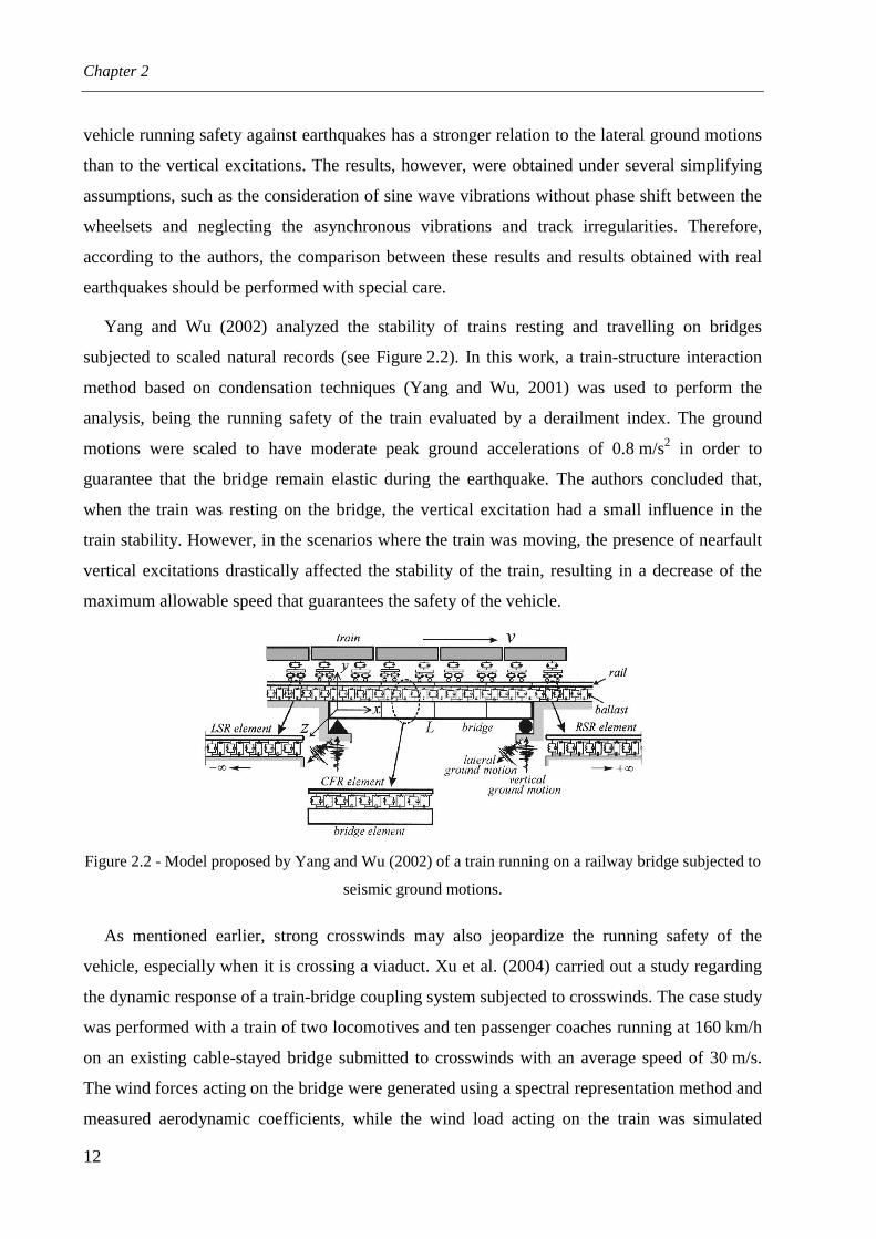
Chapter 2
12
vehicle running safety against earthquakes has a stronger relation to the lateral ground motions
than to the vertical excitations. The results, however, were obtained under several simplifying
assumptions, such as the consideration of sine wave vibrations without phase shift between the
wheelsets and neglecting the asynchronous vibrations and track irregularities. Therefore,
according to the authors, the comparison between these results and results obtained with real
earthquakes should be performed with special care.
Yang and Wu (2002) analyzed the stability of trains resting and travelling on bridges
subjected to scaled natural records (see Figure 2.2). In this work, a train-structure interaction
method based on condensation techniques (Yang and Wu, 2001) was used to perform the
analysis, being the running safety of the train evaluated by a derailment index. The ground
motions were scaled to have moderate peak ground accelerations of 0.8 m/s2 in order to
guarantee that the bridge remain elastic during the earthquake. The authors concluded that,
when the train was resting on the bridge, the vertical excitation had a small influence in the
train stability. However, in the scenarios where the train was moving, the presence of nearfault
vertical excitations drastically affected the stability of the train, resulting in a decrease of the
maximum allowable speed that guarantees the safety of the vehicle.
Figure 2.2 - Model proposed by Yang and Wu (2002) of a train running on a railway bridge subjected to
seismic ground motions.
As mentioned earlier, strong crosswinds may also jeopardize the running safety of the
vehicle, especially when it is crossing a viaduct. Xu et al. (2004) carried out a study regarding
the dynamic response of a train-bridge coupling system subjected to crosswinds. The case study
was performed with a train of two locomotives and ten passenger coaches running at 160 km/h
on an existing cable-stayed bridge submitted to crosswinds with an average speed of 30 m/s.
The wind forces acting on the bridge were generated using a spectral representation method and
measured aerodynamic coefficients, while the wind load acting on the train was simulated

State of the art
13
taking into account the effects of the vehicle speed and the spatial correlation with the wind
forces acting on the bridge. The authors evaluated the running safety of the train with the
derailment factor and with the wheel unloading criterion, concluding that the train remained
safe for the specified wind action. In fact, the differences between the derailment factor with
and without wind load were not significant for this particular case. However, according to the
authors, a parametric study would be necessary to draw more general conclusions.
Li et al. (2005) developed an analytical model for study the dynamics of the
wind-vehicle-bridge system. The model took into account several aspects regarding the wind
action, such as the fluid-solid interaction between the wind and the bridge, the stochastic
definition of the wind load and the time dependence of the system due to the movement of the
vehicle. The authors discussed the influence of the wind load in the response of the bridge and
the vehicle by comparing the results obtained in two distinct scenarios: one without crosswinds
and another with a wind load with an average speed of 25 m/s. In both scenarios, the vehicle
speed was 250 km/h. The results showed a significant increase in the lateral and vertical
accelerations of the vehicle's carbody, resulting in a variation of the vertical wheel loads due to
the rolling moments induced by the lateral wind. According to the authors, these variations in
the vertical contact forces may represent a significant threat to the vehicle's running safety.
Luo (2005) and Luo and Miyamoto (2007) made important contributions to the development
of a code-type procedure for evaluating the running safety of trains under seismic conditions.
The authors evaluated the dynamic behavior of several railway vehicles using simplified
analytical models and observed that the response of the vehicles were strongly dependent on
the frequency components of the ground motions. As a result, the authors developed a
code-type provision based on a concept of energy balance, in which the spectral intensity is
used as an assessment index for the running safety. This index, which is presented in the
Displacement Limit Standard for Railway Structures (RTRI, 2006), reflects the amount of
energy of the seismic wave that influences the vehicle vibration.
Several studies were conducted on long-span bridges subjected to earthquakes, in which the
spatial variability of the ground motion resulted in important differences in the responses when
compared with those obtained with synchronous motions at all supports (Nazmy and Abdel-
Ghaffar, 1992; Alexander, 2008). Xia et al. (2006) presented a model of the coupled
train-bridge system subjected to non-uniform excitations. In this study, the authors evaluated
the influence of the spatial variation of the ground motion in the running safety of a train
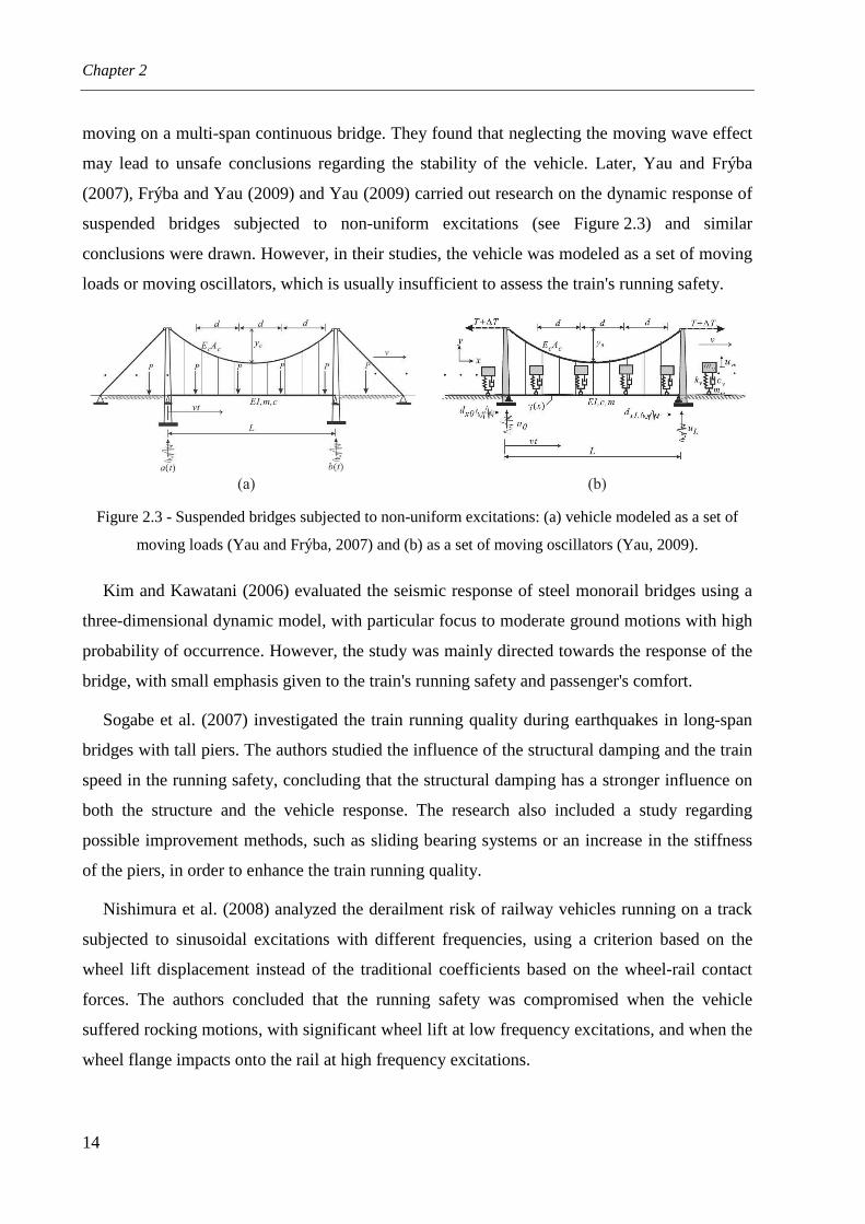
Chapter 2
14
moving on a multi-span continuous bridge. They found that neglecting the moving wave effect
may lead to unsafe conclusions regarding the stability of the vehicle. Later, Yau and Frýba
(2007), Frýba and Yau (2009) and Yau (2009) carried out research on the dynamic response of
suspended bridges subjected to non-uniform excitations (see Figure 2.3) and similar
conclusions were drawn. However, in their studies, the vehicle was modeled as a set of moving
loads or moving oscillators, which is usually insufficient to assess the train's running safety.
Figure 2.3 - Suspended bridges subjected to non-uniform excitations: (a) vehicle modeled as a set of
moving loads (Yau and Frýba, 2007) and (b) as a set of moving oscillators (Yau, 2009).
Kim and Kawatani (2006) evaluated the seismic response of steel monorail bridges using a
three-dimensional dynamic model, with particular focus to moderate ground motions with high
probability of occurrence. However, the study was mainly directed towards the response of the
bridge, with small emphasis given to the train's running safety and passenger's comfort.
Sogabe et al. (2007) investigated the train running quality during earthquakes in long-span
bridges with tall piers. The authors studied the influence of the structural damping and the train
speed in the running safety, concluding that the structural damping has a stronger influence on
both the structure and the vehicle response. The research also included a study regarding
possible improvement methods, such as sliding bearing systems or an increase in the stiffness
of the piers, in order to enhance the train running quality.
Nishimura et al. (2008) analyzed the derailment risk of railway vehicles running on a track
subjected to sinusoidal excitations with different frequencies, using a criterion based on the
wheel lift displacement instead of the traditional coefficients based on the wheel-rail contact
forces. The authors concluded that the running safety was compromised when the vehicle
suffered rocking motions, with significant wheel lift at low frequency excitations, and when the
wheel flange impacts onto the rail at high frequency excitations.
(a) (b)

State of the art
15
Baker et al. (2009) presented a state of the art of the research that has been carried out on the
crosswind effects on road and railway vehicles. Regarding the running safety of railway
vehicles, the authors stated that the main interest has been focused on the definition of the
Characteristic Wind Curves (CWC), which define the limit wind speed that leads to the
overturning of the vehicle caused by a wheel unloading of 90 %. These limits can be evaluated
through a simplified conservative approach based on a quasi-static analysis or through a
dynamic approach performed in the time domain. According to the authors, only the latter is
able to account for the effects of the contact phenomena between wheel and rail. Moreover,
only through a dynamic analysis of the vehicle, subjected to the unsteady aerodynamic forces
and moments caused by crosswinds, it is possible to make an evaluation of the effects
associated with the crosswinds other than the vehicle's rollover. In fact, turbulent crosswinds
can result in a decrease in the running safety of the vehicles if specific vibration modes are
excited. However, dynamic approaches in the time domain can be computationally expensive
and, in the majority of the cases, more complex than the quasi-static approaches.
Guo et al. (2010) studied the running safety of a train running on the Tsing Ma suspension
bridge in China, subjected to turbulent crosswinds of different speeds. The authors evaluated
the running safety of the train with two criteria from the Chinese railway design standard,
namely the derailment factor and the wheel unloading criterion, and presented the results in the
form of CWCs (see Figure 2.4). As mentioned earlier, these curves illustrate the relationships
between the mean wind velocity and the critical train speed that leads to derailment. The results
showed that the running safety was controlled by the derailment factor for wind velocities up to
15 m/s (see Figure 2.4a) and by the wheel unloading criterion for velocities above that value
(see Figure 2.4b). Furthermore, when the mean wind velocity reached 30 m/s, the critical train
speed dropped to nearly zero, indicating that the rail traffic on the bridge should be closed.
Figure 2.4 - Characteristic Wind Curves: (a) derailment factor and (b) wheel unloading criterion
(adapted from Guo et al., 2010)
0 5 10 15 20 25 30
Mean wind velocity (m/s)
400
300
200
100
0
Tra
in s
pee
d (
km
/h)
0 5 10 15 20 25 30
Mean wind velocity (m/s)
400
300
200
100
0
Tra
in s
pee
d (
km
/h)
(a) (b)
Dangerous area
Safe area Safe area
Dangerous area
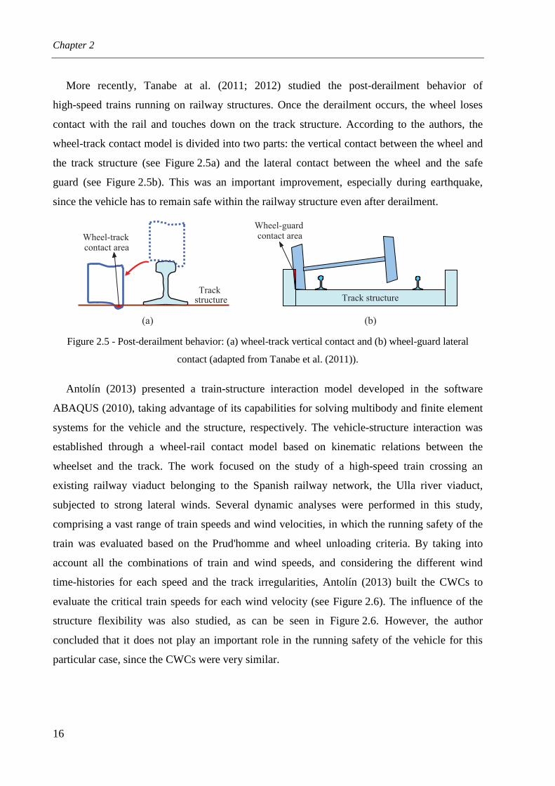
Chapter 2
16
More recently, Tanabe at al. (2011; 2012) studied the post-derailment behavior of
high-speed trains running on railway structures. Once the derailment occurs, the wheel loses
contact with the rail and touches down on the track structure. According to the authors, the
wheel-track contact model is divided into two parts: the vertical contact between the wheel and
the track structure (see Figure 2.5a) and the lateral contact between the wheel and the safe
guard (see Figure 2.5b). This was an important improvement, especially during earthquake,
since the vehicle has to remain safe within the railway structure even after derailment.
Figure 2.5 - Post-derailment behavior: (a) wheel-track vertical contact and (b) wheel-guard lateral
contact (adapted from Tanabe et al. (2011)).
Antolín (2013) presented a train-structure interaction model developed in the software
ABAQUS (2010), taking advantage of its capabilities for solving multibody and finite element
systems for the vehicle and the structure, respectively. The vehicle-structure interaction was
established through a wheel-rail contact model based on kinematic relations between the
wheelset and the track. The work focused on the study of a high-speed train crossing an
existing railway viaduct belonging to the Spanish railway network, the Ulla river viaduct,
subjected to strong lateral winds. Several dynamic analyses were performed in this study,
comprising a vast range of train speeds and wind velocities, in which the running safety of the
train was evaluated based on the Prud'homme and wheel unloading criteria. By taking into
account all the combinations of train and wind speeds, and considering the different wind
time-histories for each speed and the track irregularities, Antolín (2013) built the CWCs to
evaluate the critical train speeds for each wind velocity (see Figure 2.6). The influence of the
structure flexibility was also studied, as can be seen in Figure 2.6. However, the author
concluded that it does not play an important role in the running safety of the vehicle for this
particular case, since the CWCs were very similar.
(a) (b)
Wheel-guardcontact areaWheel-track
contact area
Track structure Track
structure

State of the art
17
Figure 2.6 - Characteristic Wind Curves: (a) flexible structure and (b) rigid structure (adapted from
Antolín (2013))
2.3 METHODS FOR ANALYZING THE DYNAMIC BEHAVIOR OF THE
STRUCTURE AND VEHICLE
In the present section, a review of the different existing methods for analyzing the dynamic
response of the structure and railway vehicles is presented. Three main methods for studying
the dynamic behavior of a railway viaduct and/or vehicle can be distinguished: 1) moving loads
model (Section 2.3.1), in which the vehicle is modeled as a set of moving loads of fixed
magnitude; 2) virtual path method (Section 2.3.2), in which the deformation of the viaduct due
to the action of the vehicle, computed with moving loads, is prescribed to the vehicle in order
to obtain its response and 3) vehicle-structure interaction methods (Section 2.3.3), in which the
viaduct and the vehicle interact with each other as a coupled dynamic system. These methods
vary in complexity, computational cost and accuracy, as will be discussed in the following
sections.
2.3.1 Moving loads model
The moving loads model is based on the assumption that the vehicle's action over the
structure may be defined by means of moving loads of fixed magnitude that represent the static
load of each wheelset (Frýba, 1996; Goicolea and Gabaldón, 2012). The train is therefore
characterized by a set of constant loads Fi, separated from each other according to the train
geometry, as shown in Figure 2.7. Hence, the interaction between the vehicle and structure is
neglected, being the method limited to the study of the dynamic response of the structure.
Safe area
Prud’homme Unloading
160 200 240 280 320
20
Train speed (km/h)
Win
d v
elo
city
(m
/s)
25
30
35
Unsafe area
(a)
Safe area
Unsafe area
20
Win
d v
elo
city
(m
/s)
25
30
35
160 200 240 280 320
Train speed (km/h)
(b)
Prud’homme Unloading
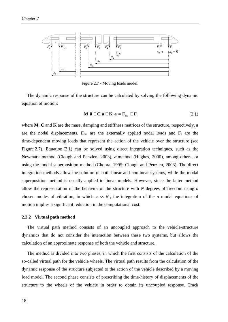
Chapter 2
18
Figure 2.7 - Moving loads model.
The dynamic response of the structure can be calculated by solving the following dynamic
equation of motion:
iext FFaKaCaM +=++ ɺɺɺ (2.1)
where M , C and K are the mass, damping and stiffness matrices of the structure, respectively, a
are the nodal displacements, Fext are the externally applied nodal loads and Fi are the
time-dependent moving loads that represent the action of the vehicle over the structure (see
Figure 2.7). Equation (2.1) can be solved using direct integration techniques, such as the
Newmark method (Clough and Penzien, 2003), α method (Hughes, 2000), among others, or
using the modal superposition method (Chopra, 1995; Clough and Penzien, 2003). The direct
integration methods allow the solution of both linear and nonlinear systems, while the modal
superposition method is usually applied to linear models. However, since the latter method
allow the representation of the behavior of the structure with N degrees of freedom using n
chosen modes of vibration, in which Nn << , the integration of the n modal equations of
motion implies a significant reduction in the computational cost.
2.3.2 Virtual path method
The virtual path method consists of an uncoupled approach to the vehicle-structure
dynamics that do not consider the interaction between these two systems, but allows the
calculation of an approximate response of both the vehicle and structure.
The method is divided into two phases, in which the first consists of the calculation of the
so-called virtual path for the vehicle wheels. The virtual path results from the calculation of the
dynamic response of the structure subjected to the action of the vehicle described by a moving
load model. The second phase consists of prescribing the time-history of displacements of the
structure to the wheels of the vehicle in order to obtain its uncoupled response. Track
. . .
. . .
. . .
1F2F
2x 1 0x =3F
3x
4x
5F6F
5x
6x
1iF −iF
1ix −
ix
4F

State of the art
19
irregularities may be added to the virtual path in order to account for their effect in the response
of the vehicle. Figure 2.8 illustrates the two aforementioned phases that compose the virtual
path method.
Figure 2.8 - Virtual path method: (a) phase 1 and (b) phase 2.
Unlike the moving load model, this method allows the calculation, though simplified, of the
response of the vehicle. However, the interaction between the structure and the vehicle may be
significant in some cases. Furthermore, the study of the riding comfort of passengers or running
safety of trains requires more complex models, which usually includes the effects of the
wheel-rail contact. Such effects cannot be captured by this method, limiting it to simplified
analysis for obtaining a first estimate of the response of the vehicle. A study involving the
virtual path method may be found in Goicolea and Antolín (2011).
2.3.3 Vehicle-structure interaction methods
2.3.3.1 Iterative method
The iterative method is a widely used technique to solve the vehicle-structure interaction
problem (Hwang and Nowak, 1991; Yang and Fonder, 1996; Delgado and Santos, 1997; Lei
and Noda, 2002; Xia et al., 2008; Nguyen et al., 2009a; Lee and Kimb, 2010). This method
establishes the equilibrium of forces acting on the contact interface and uses an iterative
procedure to impose the constraint equations that relate the displacements of the contact nodes
of the vehicle with the corresponding displacements of the structure.
The two subsystems, the vehicle and structure, are modeled as two separate substructures,
whose decoupled governing equilibrium equations may be expressed as
=
+
+
V
S
V
S
V
S
V
S
V
S
V
S
V
S
F
F
a
a
K0
0K
a
a
C0
0C
a
a
M0
0Mɺ
ɺ
ɺɺ
ɺɺ (2.2)
Moving loads
x
z y
Structure system Vehicle system
(virtual path)
ya
zazaya
Structure response Prescribe virtual pathto the train wheels
(a) (b)
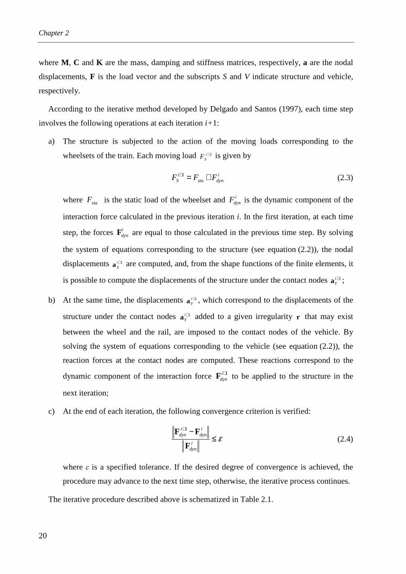
Chapter 2
20
where M , C and K are the mass, damping and stiffness matrices, respectively, a are the nodal
displacements, F is the load vector and the subscripts S and V indicate structure and vehicle,
respectively.
According to the iterative method developed by Delgado and Santos (1997), each time step
involves the following operations at each iteration i+ 1:
a) The structure is subjected to the action of the moving loads corresponding to the
wheelsets of the train. Each moving load 1+iSF is given by
idynsta
iS FFF +=+1 (2.3)
where staF is the static load of the wheelset and idynF is the dynamic component of the
interaction force calculated in the previous iteration i. In the first iteration, at each time
step, the forces idynF are equal to those calculated in the previous time step. By solving
the system of equations corresponding to the structure (see equation (2.2)), the nodal
displacements 1+iSa are computed, and, from the shape functions of the finite elements, it
is possible to compute the displacements of the structure under the contact nodes 1+iYa ;
b) At the same time, the displacements 1+iVa , which correspond to the displacements of the
structure under the contact nodes 1+iYa added to a given irregularity r that may exist
between the wheel and the rail, are imposed to the contact nodes of the vehicle. By
solving the system of equations corresponding to the vehicle (see equation (2.2)), the
reaction forces at the contact nodes are computed. These reactions correspond to the
dynamic component of the interaction force 1+idynF to be applied to the structure in the
next iteration;
c) At the end of each iteration, the following convergence criterion is verified:
ε≤−+
idyn
idyn
idyn
F
FF 1
(2.4)
where ε is a specified tolerance. If the desired degree of convergence is achieved, the
procedure may advance to the next time step, otherwise, the iterative process continues.
The iterative procedure described above is schematized in Table 2.1.
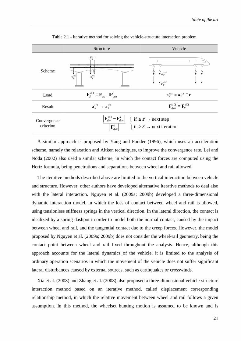
State of the art
21
Table 2.1 - Iterative method for solving the vehicle-structure interaction problem.
Structure Vehicle
Scheme
Load idynsta
iS FFF +=+1 raa += ++ 11 i
YiV
Result 11 ++ → iY
iS aa 11 ++ = i
Vi
dyn FF
Convergence criterion
→>→≤−+
iterationnext if
stepnext if1
εε
idyn
idyn
idyn
F
FF
A similar approach is proposed by Yang and Fonder (1996), which uses an acceleration
scheme, namely the relaxation and Aitken techniques, to improve the convergence rate. Lei and
Noda (2002) also used a similar scheme, in which the contact forces are computed using the
Hertz formula, being penetrations and separations between wheel and rail allowed.
The iterative methods described above are limited to the vertical interaction between vehicle
and structure. However, other authors have developed alternative iterative methods to deal also
with the lateral interaction. Nguyen et al. (2009a; 2009b) developed a three-dimensional
dynamic interaction model, in which the loss of contact between wheel and rail is allowed,
using tensionless stiffness springs in the vertical direction. In the lateral direction, the contact is
idealized by a spring-dashpot in order to model both the normal contact, caused by the impact
between wheel and rail, and the tangential contact due to the creep forces. However, the model
proposed by Nguyen et al. (2009a; 2009b) does not consider the wheel-rail geometry, being the
contact point between wheel and rail fixed throughout the analysis. Hence, although this
approach accounts for the lateral dynamics of the vehicle, it is limited to the analysis of
ordinary operation scenarios in which the movement of the vehicle does not suffer significant
lateral disturbances caused by external sources, such as earthquakes or crosswinds.
Xia et al. (2008) and Zhang et al. (2008) also proposed a three-dimensional vehicle-structure
interaction method based on an iterative method, called displacement corresponding
relationship method, in which the relative movement between wheel and rail follows a given
assumption. In this method, the wheelset hunting motion is assumed to be known and is
1i
Ya +
1i
SF +
1i
Sa +
1i
Va +
1i
VF +

Chapter 2
22
regarded as a lateral excitation to the vehicle. This excitation is imposed at the wheels as a
prescribed displacement ha , which can be expressed approximately as (Dukkipati, 2000; Yang
et al., 2004)
( )
+= h
hhh
xAxa φ
λπ2
cos (2.5)
where hA , hλ and hφ are the hunting amplitude, wavelength and random phase angle,
respectively. The system of equations (2.2) is solved using a direct integration technique, in
which the displacement corresponding relationship between the vehicle and structure systems is
determined iteratively. As in the aforementioned approach proposed by Nguyen et al. (2009a;
2009b), this model is restricted to the analysis of scenarios in ordinary operating conditions,
since it cannot predict the response of the vehicle due to other actions besides the hunting
motion.
2.3.3.2 Condensation method
Yang and Yau (1997) developed a finite element called vehicle-bridge interaction element
(see Figure 2.9a) that, according to the authors, is both accurate and efficient for modeling the
vehicle-bridge interaction. Yang and Yau (1997) modeled the vehicle as a sequence of lumped
sprung masses, the bridge with beam elements and the track with lumped masses, springs and
dashpot elements to simulate the ballast behavior. The method consists firstly of formulating
the two equations of motion of the system, one for the bridge and another for the lumped
sprung masses forming the vehicle. The vehicle equation is then discretized using Newmark's
finite difference formulas, being its degrees of freedom condensed into the bridge elements that
are in contact. Since the vehicle is modeled as a series of sprung masses, the resulting
interaction element ignores the pitching effect of the vehicle, which may significantly affect the
response of the whole system. Therefore, Yang et al. (1999) presented an improved interaction
element, in which the vehicle is modeled with a rigid beam supported by two spring-dampers
(see Figure 2.9b), and later, Yang and Wu (2001) and Wu et al. (2001) developed a procedure
capable of simulating vehicles of varying complexity, as shown in Figure 2.9c. The detailed
formulation of the different versions of the interaction element, as well as a series of
applications on high-speed railways may be found in Yang et al. (2004).

State of the art
23
(a) (b)
(c)
Figure 2.9 - Vehicle-bridge interaction elements: (a) original element, (b) element considering the
pitching effect and (c) vehicle with an higher degree of complexity (Yang et al., 2004).
The so-called vehicle-bridge interaction element, which results from this procedure based on
condensation techniques, preserve the properties of symmetry and bandwidth. However, since
the position of each contact point changes over time, the system matrix used in this method is
usually time-dependent and must be updated and factorized at each time step, which may
demand a considerable computational effort.
2.3.3.3 Direct method
Neves et al. (2012) proposed a new algorithm, referred to as the direct method, in which the
governing equilibrium equations of the vehicle and structure are complemented with additional
constraint equations that relate the displacements of the contact nodes of the vehicle with the
corresponding nodal displacements of the structure, with no separation being allowed. The
irregularities at the contact interface can be considered in the constraint equations and the
vehicle and structure subsystems may be modeled with various types of finite elements with
any degree of complexity, such as beams, springs, shells, and solids, as shown in Figure 2.10.
Railirregularity
Ballast stiffness kb
z
y
xL
mw
cvkv
y1
y2
Mv
v
y
z
x
Rail
element ielement j
mw
cv
Iv
Mv
v
yv
θv
kv
L
mw
cvkv
irregularity
train
track
bridge element
LSR element RSR element
central track segment
bridge segment
left track segment right track segment
CFR element

Chapter 2
24
Figure 2.10 - Vehicle-structure interaction system: (a) schematic illustration and (b) free body diagram
(Neves et al., 2012).
The equations of motion and the constraint equations form a single system, with
displacements and contact forces as unknowns, that is solved directly using an optimized block
factorization algorithm, thus avoiding the iterative procedure describe in Section 2.3.3.1 to
satisfy the constraint equations. The single system of linear equations is expressed in matrix
form as
=
∆+
∆+
r
F
X
a
0H
DK F
tt
ttF
XF
FXFF (2.6)
where FFK is the effective stiffness matrix of the vehicle-structure system, FXD and XFH are
transformation matrices that relate, respectively, the contact forces in the local coordinate
system with the nodal forces in the global coordinate system and the nodal displacements of the
structure in the global coordinate system with the displacements of the auxiliary points defined
in the local coordinate system, ttF
∆+a and tt ∆+X are the nodal displacements and contact forces,
respectively, at the current time step, FF is the load vector and r are the irregularities at the
contact interface.
Later, Neves et al. (2014) extended the formulation to allow the separation between wheel
and rail, by developing a contact search algorithm that detects which elements are in contact,
being the constraints imposed only when contact occurs. Since in this formulation only
frictionless contact is considered, the constraint equations are purely geometric and relate the
displacements of the contact node with the displacements of the corresponding target element.
Due to the nonlinear nature of the contact problem, an iterative scheme based on the Newton
method (Owen and Hinton, 1980; Bathe, 1996) is used to solve the equation of motion of the
Structure
v t( )
r1r2
X1
X2
(a) (b)
X1 X2
Vehicle

State of the art
25
vehicle-structure system. Thus, the system of equations (2.6) is rewritten in an incremental
form as
( )
=
∆∆
∆+∆+
+
+
r
X,aψ
X
a
0H
DK ittittF
i
iF
XF
FXFF,,
1
1
(2.7)
where 1+∆ iFa and 1+∆ iX are the incremental nodal displacements and contact forces,
respectively, at the current iteration and ψ is the residual force vector, which depends on the
nodal displacements and contact forces calculated in the previous Newton iteration. The
iterative scheme continues until the condition
( )
ε≤∆+
+∆++∆+
ttF
ittittF
P
Xaψ 1,1, , (2.2.8)
is fulfilled, where ttF
∆+P is the vector of the external applied loads at the current time step and ε
is a specified tolerance. Note that the iterative procedure used in this method is not related with
the compatibility of displacements between vehicle and structure, as shown in the methods
described in Section 2.3.3.1, but with the nonlinear nature of the contact due to the
consideration of contact loss.
2.3.3.4 Methods considering the wheel and rail geometries
The methods mentioned in the previous sections are restricted to railway dynamic analysis
under ordinary operating conditions, since they cannot deal with extreme scenarios, such as
strong lateral winds or earthquakes, in which the lateral impacts between wheel flange and rail
may strongly influence the dynamic behavior of the system. To overcome this limitation, the
geometries of the wheel and rail profiles have to be taken into account and a fully nonlinear
formulation has to be used. In wheel-rail contact problems, since the normal and tangential
forces significantly depend on the geometric characteristics of the surfaces near the contact
point, the accuracy used for defining these surfaces is crucial.
According to Shabana et al. (2008), the formulation of the wheel-rail contact problem may
be classified in two different approaches in terms of the way the normal contact forces are
computed. In the first approach, named constraint contact formulation (Shabana et al., 2001),
nonlinear kinematic constraints are used to impose the contact conditions, where the
penetration between the wheel and the rail is not allowed. By imposing these constraints using,
for example, the Lagrange multipliers method or the penalty method (Wriggers, 2002), one

Chapter 2
26
degree of relative motion between wheel and rail is eliminated and the normal contact force is
calculated as a constraint force. In the second approach, however, no degrees of freedom are
eliminated, being the normal contact force defined as function of the penetration between wheel
and rail, using any of the normal contact theories described later in Section 2.4.2. This
approach is called elastic contact formulation and it is adopted by many authors, such as
Shabana et al. (2004), Pombo et al. (2007), Tanabe et al. (2008), Sugiyama and Suda (2009),
Zhai et al. (2009), Du et al. (2012) or Antolín (2013).
Another distinction that is usually made between formulations that take into account the
profile geometries is related with the algorithm used to locate the contact point position.
According to Sugiyama et al. (2009), there are two different approaches for determining the
contact points between wheel and rail. They are the offline contact search, in which the
location of the contact points is precalculated through a contact geometry analysis and stored in
a contact lookup table to be later interpolated during the dynamic analysis, and the online
contact search, where the position of the contact points is computed during the dynamic
analysis using iterative procedures at every time step. A more detailed discussion about these
two approaches is presented in Section 2.4.1.
Despite the method used to deal with the coupling between wheel and rail, the formulations
which take into account the geometry of the wheel and rail profiles are the most suitable and
accurate to deal with railway dynamics.
2.4 WHEEL-RAIL CONTACT MODELS
In the present section, an overview of the existing wheel-rail contact models is presented.
The location of contact points between wheel and rail and the consequent calculation of the
contact forces that are generated in the contact interface is one of the most important issues in
railway dynamics. Therefore, several approaches varying in complexity can be found in the
literature to solve the wheel-rail contact problem. The wheel-rail contact models are generally
divided into three main steps: 1) the geometric problem (Section 2.4.1), consisting of the
detection of the contact points; 2) the normal contact problem (Section 2.4.2), in which the
normal contact forces are computed, and 3) the tangential contact problem (Section 2.4.3),
where the creep forces that appear due to the rolling friction contact are calculated. The
different approaches that can be found in the literature for solving each of these problems are
described in the following sections.
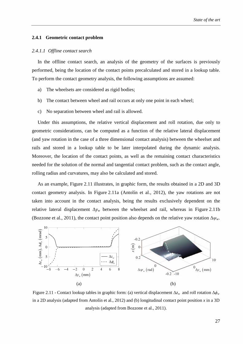
State of the art
27
2.4.1 Geometric contact problem
2.4.1.1 Offline contact search
In the offline contact search, an analysis of the geometry of the surfaces is previously
performed, being the location of the contact points precalculated and stored in a lookup table.
To perform the contact geometry analysis, the following assumptions are assumed:
a) The wheelsets are considered as rigid bodies;
b) The contact between wheel and rail occurs at only one point in each wheel;
c) No separation between wheel and rail is allowed.
Under this assumptions, the relative vertical displacement and roll rotation, due only to
geometric considerations, can be computed as a function of the relative lateral displacement
(and yaw rotation in the case of a three dimensional contact analysis) between the wheelset and
rails and stored in a lookup table to be later interpolated during the dynamic analysis.
Moreover, the location of the contact points, as well as the remaining contact characteristics
needed for the solution of the normal and tangential contact problem, such as the contact angle,
rolling radius and curvatures, may also be calculated and stored.
As an example, Figure 2.11 illustrates, in graphic form, the results obtained in a 2D and 3D
contact geometry analysis. In Figure 2.11a (Antolín et al., 2012), the yaw rotations are not
taken into account in the contact analysis, being the results exclusively dependent on the
relative lateral displacement ∆yw between the wheelset and rail, whereas in Figure 2.11b
(Bozzone et al., 2011), the contact point position also depends on the relative yaw rotation ∆ψw.
(a) (b)
Figure 2.11 - Contact lookup tables in graphic form: (a) vertical displacement ∆zw and roll rotation ∆ϕw
in a 2D analysis (adapted from Antolín et al., 2012) and (b) longitudinal contact point position x in a 3D
analysis (adapted from Bozzone et al., 2011).
( )mmwy∆
wz∆
wφ∆
()
()
mm
,m
rad
ww
zφ
∆∆
( )mmwy∆
10
-10( )radwψ∆
-0.2
0.2
-0.2
0 0
0()
mx

Chapter 2
28
This approach is computationally attractive, since it does not require any additional
calculation during the dynamic analysis other than the table interpolation. However, it does not
account for the penetration between the wheel and the rail, which may have a significant
influence in the computation of the contact forces. This limitation is overcome in the online
contact approach described in the next section. Several studies using the offline contact search
may be found in Santamaria et al. (2006), Tanabe et al. (2008), Bozzone et al. (2011) and
Antolín et al. (2012).
2.4.1.2 Online contact search
In the online contact search, the location of contact points is determined during the dynamic
simulation using iterative procedures at every time step. Since the location of the contact points
is predicted directly with the information of the current time step, a more accurate solution is
usually achieved in comparison with that obtained using the offline search. Furthermore, the
online contact search does not require the wheelset to be rigid, allowing the detection of contact
points in vehicles with independent wheels or flexible wheelsets. Two other important
advantages of this approach consists in the possibility of considering small penetrations
between the wheel and rail, essential for the accuracy of the normal contact forces calculation,
and of detecting multiple contact points in the same wheel-rail pair.
Figure 2.12 illustrates two approaches for predicting the location of the contact points using
an online contact search. In Figure 2.12a, the contact point is determined based on a nodal
search algorithm, in which the geometric surfaces are discretized in several points, being the
contact point formed by the nodal pair that leads to the maximum indentation (Chen and Zhai,
2004; Shabana et al., 2005; Antolín, 2013). In Figure 2.12b however, the profile surfaces are
described by mathematical functions and the contact point position is determined by solving a
set of nonlinear algebraic equations that define the geometric contact conditions based on the
normal and tangential vectors to the surfaces (Pombo et al., 2007; Shabana et al., 2008;
Sugiyama and Suda, 2009; Falomi et al., 2010). The latter method is computationally more
efficient than the nodal search algorithm and its accuracy does not depend on the degree of
discretization of the profile geometry. However, multiple solutions can be obtained for the
system of nonlinear equations if one of the contact surfaces is not convex (Pombo, 2004). This
can be an important limitation if the potential contact point lies on the concave region that exist
in the transition between the wheel tread and flange.
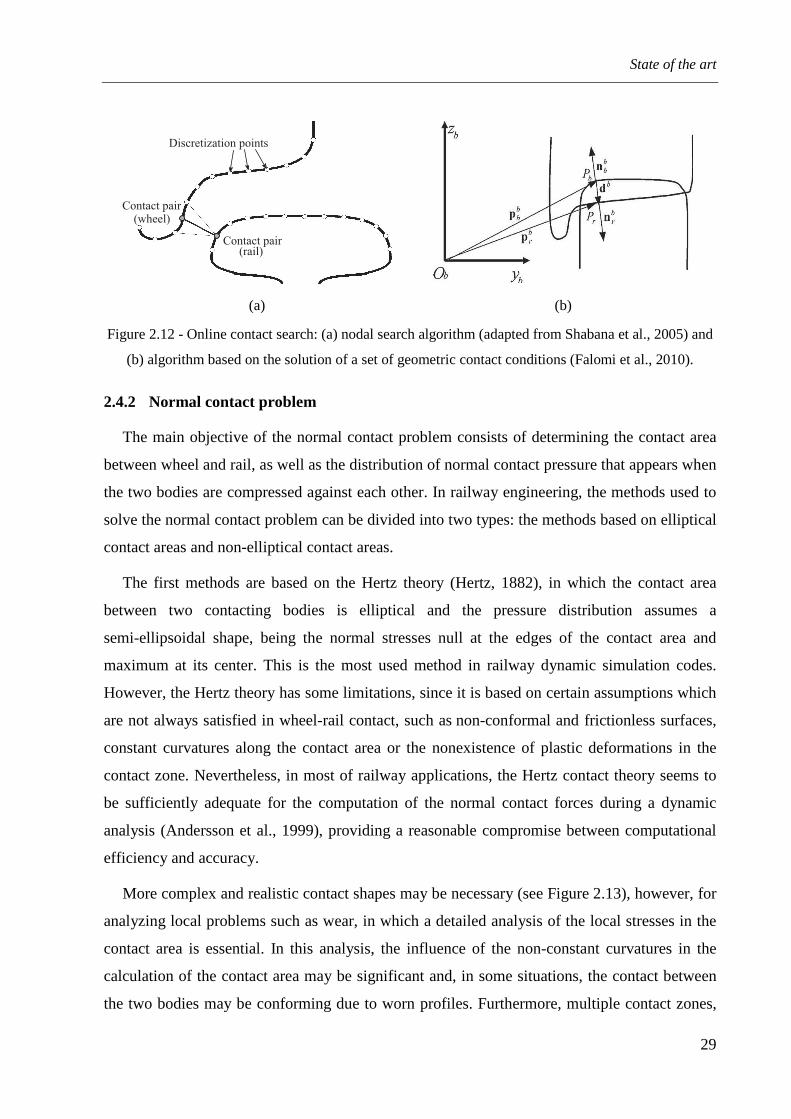
State of the art
29
(a) (b)
Figure 2.12 - Online contact search: (a) nodal search algorithm (adapted from Shabana et al., 2005) and
(b) algorithm based on the solution of a set of geometric contact conditions (Falomi et al., 2010).
2.4.2 Normal contact problem
The main objective of the normal contact problem consists of determining the contact area
between wheel and rail, as well as the distribution of normal contact pressure that appears when
the two bodies are compressed against each other. In railway engineering, the methods used to
solve the normal contact problem can be divided into two types: the methods based on elliptical
contact areas and non-elliptical contact areas.
The first methods are based on the Hertz theory (Hertz, 1882), in which the contact area
between two contacting bodies is elliptical and the pressure distribution assumes a
semi-ellipsoidal shape, being the normal stresses null at the edges of the contact area and
maximum at its center. This is the most used method in railway dynamic simulation codes.
However, the Hertz theory has some limitations, since it is based on certain assumptions which
are not always satisfied in wheel-rail contact, such as non-conformal and frictionless surfaces,
constant curvatures along the contact area or the nonexistence of plastic deformations in the
contact zone. Nevertheless, in most of railway applications, the Hertz contact theory seems to
be sufficiently adequate for the computation of the normal contact forces during a dynamic
analysis (Andersson et al., 1999), providing a reasonable compromise between computational
efficiency and accuracy.
More complex and realistic contact shapes may be necessary (see Figure 2.13), however, for
analyzing local problems such as wear, in which a detailed analysis of the local stresses in the
contact area is essential. In this analysis, the influence of the non-constant curvatures in the
calculation of the contact area may be significant and, in some situations, the contact between
the two bodies may be conforming due to worn profiles. Furthermore, multiple contact zones,
Discretization points
Contact pair
Contact pair(wheel)
(rail)

Chapter 2
30
which cannot be solved using a single ellipse, may appear when the geometry of the contacting
bodies does not satisfy the Hertz assumptions. Therefore, several authors have developed new
theories to deal with these limitations, which, according to Piotrowski and Chollet (2005), can
be divided into the following two categories:
a) Multi-Hertzian methods: the Hertz theory is applied to each contact zone, forming a
contact area with multiple ellipses;
b) Non-Hertzian methods: assume a semi-elliptical distribution of stresses only along the
direction of rolling.
The multi-Hertzian methods (Pascal, 1993; Ayasse et al., 2000) are based on the fact that, in
each contact zone, the conditions for using the Hertz theory are met. Under this assumption, the
contact problem may be solved using multiple ellipses whose dimensions and pressure
distribution are obtained independently.
In the non-Hertzian methods proposed, for example, by Ayasse and Chollet (2005), Quost et
al. (2006) or Piotrowski and Kik (2008), a semi-elliptical normal stress distribution is assumed
only in the rolling direction. The similarity of the stress distribution to that resulting from the
Hertz theory allows the use of the Hertz solution to solve, in an approximate way, the normal
contact problem for conditions in which the geometry of the contacting bodies does not
rigorously satisfy the Hertz assumptions. Generally, the contact area is discretized into
independent longitudinal strips with constant curvature, allowing the consideration of both
elliptical and non-elliptical contact shapes.
Figure 2.13 - Contact area based on a multi-Hertzian and on a non-Hertzian method
(adapted from Quost et al. (2006)).
8
y (mm)
x (
mm
)
-20 -15 -10 -5 0 5 10 15 20
6
4
2
0
-2
-4
-6
-8
Multi-Hertzian
Non-Hertzian

State of the art
31
2.4.3 Tangential contact problem
If two bodies that are compressed against each other are allowed to roll over each other,
some points on the contact area may slip while others may adhere. The difference between the
tangential strains of the bodies in the adhesion area leads to a small apparent slip, called creep.
The creep, which depends on the relative velocities of the two bodies at the contact point, is
crucial for the determination of the tangential forces that are developed in the contact area,
called creep forces. Hence, the creep may be defined as a combined elastic and frictional
behavior in which two elastic bodies that roll over each other share a contact area where both
slip and adhesion occur simultaneously.
Several creep force theories were developed and implemented in many simulation softwares
for dynamic analysis of railway vehicles. The first theory was developed by Carter (1926) to
deal with two-dimensional problems. After that, Johnson (1958) extended Carter's theory to the
three-dimensional case of two spheres without spin and, later, Vermeulen and Johnson (1964)
developed a new extension to deal with smooth half-spaces, also without spin. This drawback
was overcome by Kalker (1967) with the development of the linear theory of rolling contact.
However, this theory is limited to small creepages, since it is assumed that the slip region is
very small and its effect can be neglected.
Since the wheel-rail contact problem is highly nonlinear, the aforementioned linear theories
have strong limitations when dealing with real problems. The Johnson and Vermeulen's theory
ignores the effect of the spin creepage, which may be important, especially when flange contact
occurs (Piotrowski, 1982), while Kalker's linear theory is limited to small creepages. Therefore,
new nonlinear rolling contact theories have been developed to allow more realistic studies.
In 1979, Kalker (1979) developed the exact theory of rolling contact, also called variational
theory, in which the constitutive law is obtained by deriving the tangential displacement-stress
relationship using the general elasticity theory. This formulation was first implemented in the
computer code DUVOROL (Kalker, 1979) for dealing with contact problems limited to
elliptical contact areas and later, in 1982, in the program CONTACT (Kalker, 1982b) to solve
any type of contact problem between bodies that could be described by half-spaces. However,
despite the solution for the wheel-rail contact problem given by this formulation is exact, its
excessive computational cost makes it impracticable to be used in dynamic analysis of railway
vehicles. Therefore, Kalker (1982a) developed the simplified theory to overcome the excessive
computational effort required by the exact theory and implemented it in the FASTSIM code.
Chapter 2
32
The main difference of the Kalker's simplified theory in relation to the exact theory consists in
the adoption of a much simpler tangential displacement-stress relationship. Nevertheless, the
calculation time required by the simplified theory may still be too high in certain complex
systems.
Shen et al. (1983) developed the heuristic nonlinear creep force model, in which the creep
forces calculated by the Kalker's linear theory are corrected by a reduction coefficient based on
the nonlinear creep force saturation law of Johnson and Vermeulen. However, although the
effect of spin creepage on the creep forces is considered and the computational cost is low,
Kalker (1991) stated that the heuristic theory leads to unsatisfactory results in the case of high
values of spin.
Some of the aforementioned drawbacks were overcome by the Polach method (Polach,
1999) and the Kalker's book of tables (Kalker, 1996), implemented in the USETAB code. In
spite of the simplifications used in Polach's formulation, the spin effect is considered and, in
comparison to other approximate methods, the differences observed between the calculated
values and the exact theory are relatively small. Regarding the Kalker's book of tables, it
consists in a precalculated table that is generated based on the exact theory, and which may be
interpolated during the dynamic analysis. The estimate error resulting from USETAB is
approximately 1.5 % compared with the exact theory (Shabana et al., 2008). An overview of
the wheel-rail rolling contact theories developed by Kalker may be found in the publication of
Zaazaa and Schwab (2009).
2.5 NORMS AND RECOMMENDATIONS CONCERNING THE SAFETY OF
RAILWAY TRAFFIC
2.5.1 Introduction
The majority of the existing standards regarding the design of railway bridges are mainly
focused on the structural safety, both in terms of ultimate limit states and service limit states.
However, few recommendations regarding the running safety of the railway vehicles during
ordinary operating conditions or during the occurrence of less probable events, such as
earthquakes or strong crosswinds, have been proposed so far. The present section summarizes
some of the main criteria regarding the stability and running safety of trains on railway
viaducts, defined in the standards from Europe, Japan and U.S.A.

State of the art
33
2.5.2 European standards
In Europe, the main criteria regarding the stability of the track and, consequently, the
stability of railway vehicles, are presented in the EN 1990‑Annex A2 (2001) and in the
EN 1991‑2 (2003). The verifications defined by these standards are primary related with the
control of deformations (see Section 2.5.2.1) and vibrations on bridges (see Section 2.5.2.2),
since, according to EN 1990‑Annex A2 (2001), “Excessive bridge deformations can endanger
traffic by creating unacceptable changes in vertical and horizontal track geometry, excessive
rail stresses and vibrations in bridge structures”. Moreover, “Excessive vibrations can lead to
ballast instability and unacceptable reduction in wheel rail contact forces”.
The Technical Specifications for Interoperability in Europe (TSI, 2002) and the EN 14067-6
(2010) also define criteria to guarantee the running safety of trains in the European railway
network. These criteria are mostly related with the control of the wheel-rail contact forces, as
described in Section 2.5.2.3.
2.5.2.1 Criteria regarding the bridge deformation control
2.5.2.1.1 Vertical deflection of the deck
The limitation of the vertical deflection of the deck in each span is designed to ensure an
acceptable vertical track radii and generally robust structures. Thus, according to
EN 1990‑Annex A2 (2001), the maximum total vertical deflection δv (see Figure 2.14)
measured along the track due to the characteristic values of the vertical traffic load models
LM71 and SW/0, as appropriate1, defined in EN 1991‑2 (2003), cannot exceed L/600, where L
is the span length.
Figure 2.14 - Vertical deflection of the deck δv.
1 For continuous bridges, both the load model LM71 and SW/0 have to be considered in the design.
L
LM71SW/0
600v Lδ ≤

Chapter 2
34
2.5.2.1.2 Transverse deflection of the deck
According to EN 1990‑Annex A2 (2001), the transversal deflection of the deck δh has to be
limited to ensure that the angular variation and horizontal radius of curvature satisfy the limits
specified in Table 2.2. The angular variations refer to the transversal rotations at the end of the
deck θh or to the relative transversal rotations between two adjacent spans θh1 + θh2, as depicted
in Figure 2.15. This condition has to be checked for characteristic combinations of: load model
LM71 and SW/0, as appropriate, multiplied by the dynamic factor, wind loads, nosing force,
centrifugal forces in accordance with EN 1991‑2 (2003) and the effect of transverse differential
temperature across the bridge.
Figure 2.15 - Transverse deflection of the deck δh and angular variations at the deck ends θh (plan view).
Table 2.2 - Design limit values of angular variation and radius of curvature (EN 1990-Annex A2, 2001).
Speed V (km/h) Maximum
angular variation (rad)
Maximum radius of curvature (m)
Single span Multi-span
V ≤ 120 0.0035 1700 3500
120 < V ≤ 200 0.0020 6000 9500
V > 200 0.0015 14000 17500
2.5.2.1.3 Deck twist
The deck twist criterion defined in EN 1990‑Annex A2 (2001) aims to minimize the risk of
train derailment. The maximum twist t (see Figure 2.16) of a track gauge of 1435 mm measured
over a length of 3 m should not exceed the values given in Table 2.3. The twist of the bridge
deck is calculated taking into account the characteristic values of the load model LM71, as well
as the load models SW/0 or SW/2, as appropriate, and the High-Speed Load Models (HSLM)
including centrifugal effects, as defined in EN 1991‑2 (2003).
L
hδ
hθ
h1θ h2θ
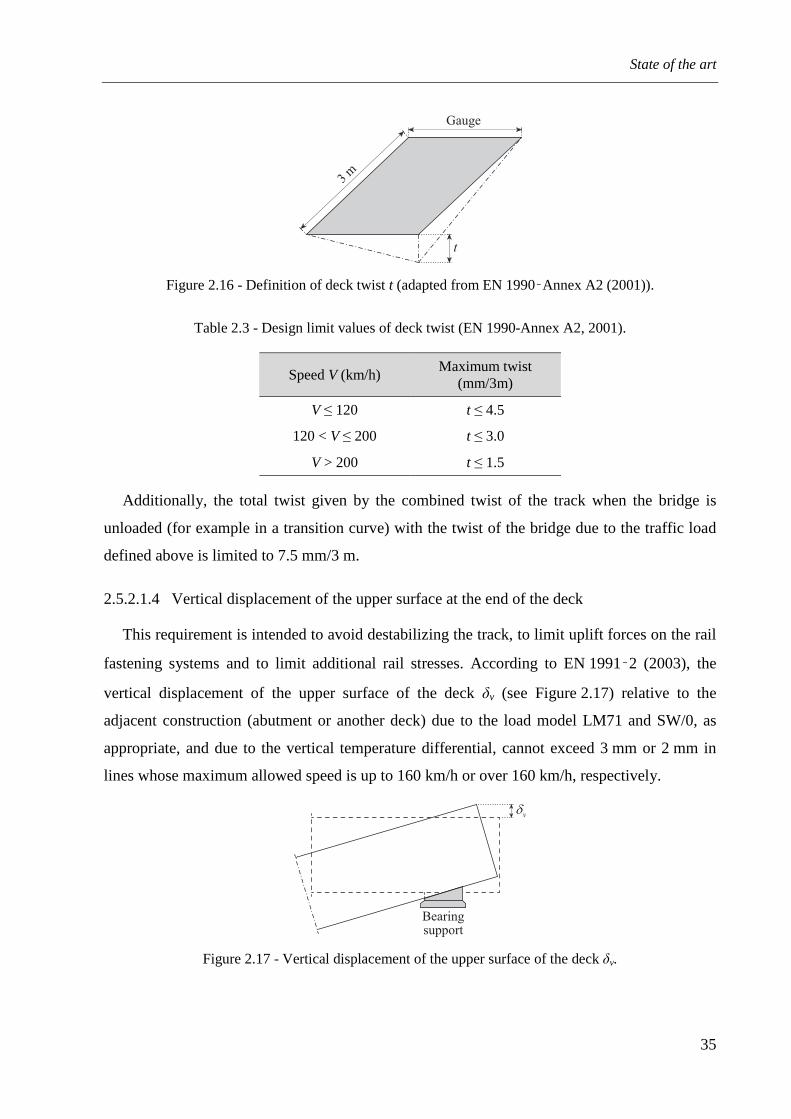
State of the art
35
Figure 2.16 - Definition of deck twist t (adapted from EN 1990‑Annex A2 (2001)).
Table 2.3 - Design limit values of deck twist (EN 1990-Annex A2, 2001).
Speed V (km/h) Maximum twist
(mm/3m)
V ≤ 120 t ≤ 4.5
120 < V ≤ 200 t ≤ 3.0
V > 200 t ≤ 1.5
Additionally, the total twist given by the combined twist of the track when the bridge is
unloaded (for example in a transition curve) with the twist of the bridge due to the traffic load
defined above is limited to 7.5 mm/3 m.
2.5.2.1.4 Vertical displacement of the upper surface at the end of the deck
This requirement is intended to avoid destabilizing the track, to limit uplift forces on the rail
fastening systems and to limit additional rail stresses. According to EN 1991‑2 (2003), the
vertical displacement of the upper surface of the deck δv (see Figure 2.17) relative to the
adjacent construction (abutment or another deck) due to the load model LM71 and SW/0, as
appropriate, and due to the vertical temperature differential, cannot exceed 3 mm or 2 mm in
lines whose maximum allowed speed is up to 160 km/h or over 160 km/h, respectively.
Figure 2.17 - Vertical displacement of the upper surface of the deck δv.
Gauge
t
3 m
vδ
Bearing support

Chapter 2
36
2.5.2.1.5 Longitudinal displacement of the upper surface at the end of the deck
The longitudinal displacement of the upper surface at the end of the deck has to be limited to
minimize disturbance to track ballast and adjacent track formation. EN 1991‑2 (2003) limits
the longitudinal displacement of the deck δb relative to the adjacent construction (abutment or
another deck) due to traction or braking to 5 mm for continuous welded rails without expansion
devices or to 30 mm for rails with expansion devices. For vertical traffic loading defined by the
load model LM71 and SW/0, as appropriate, the longitudinal displacement δh (see Figure 2.18)
of the upper surface at the end of the deck cannot exceed 8 mm if the combined behavior of
structure and track is considered in the numerical model or 10 mm if not.
Figure 2.18 - Longitudinal displacement of the upper surface of the deck δh: (a) fixed support and
(b) guided support.
2.5.2.2 Criteria regarding the bridge vibration control
2.5.2.2.1 Vertical acceleration of the deck
To ensure traffic safety, the verification of maximum vertical peak deck acceleration due to
the rail traffic loads should be regarded as a traffic safety requirement at the serviceability limit
state for the prevention of track instability. Therefore, according to EN 1990‑Annex A2 (2001),
the maximum allowed vertical acceleration of the bridge deck should not exceed 3.5 m/s2 on
ballasted tracks and 5 m/s2 on slab tracks.
The acceleration is calculated by a dynamic analysis with real high-speed train models and
with the load models HSLM, defined in EN 1991‑2 (2003), considering only one loaded track.
In the calculations, only the contributions of the mode shapes with frequencies up to 30 Hz or
to 1.5 times the frequency of the first mode of vibration of the element being analyzed,
including at least the first three modes, should be taken into account.
(a) (b)
hδ hδ

State of the art
37
2.5.2.2.2 Lateral vibration of the deck
This requirement is intended to avoid the occurrence of resonance between the lateral
motion of the vehicle and the bridge. According to EN 1990‑Annex A2 (2001), the first natural
frequency of lateral vibration of a span should not be less than 1.2 Hz.
2.5.2.3 Criteria regarding the control of the wheel-rail contact forces
2.5.2.3.1 Maximum dynamic vertical wheel load
According to TSI (2002), the maximum dynamic vertical wheel load applied by
interoperable high-speed trains should not exceed the values given in Table 2.4.
Table 2.4 - Limit values for the dynamic vertical wheel load (adapted from TSI (2002)).
Maximum Speed V (km/h)
Maximum dynamic wheel load (kN)
200 < V ≤ 250 180
250 < V ≤ 300 170
V > 300 160
2.5.2.3.2 Maximum total dynamic lateral contact force applied by a wheelset
The maximum total dynamic lateral contact force applied by a wheelset should be limited to
avoid track damage and consequent instability of the vehicle. Therefore, the maximum allowed
dynamic lateral force Ymax applied by a wheelset is given by (TSI, 2002)
[ ]kN3
210 0
max
QY
ws
+=∑ (2.9)
where Q0 is the static load per wheel in kilonewtons and ws indicates wheelset. This criterion
was firstly introduced by Prud'homme (1967) and is widely adopted in railway engineering (see
Section 3.5 of Chapter 3 for a detailed description of the Prud'homme criterion).
2.5.2.3.3 Ratio of the lateral to the vertical contact forces of a wheel
The TSI (2002) also specifies a limit for the ratio of the lateral to the vertical contact forces
of a wheel. This ratio was firstly introduced by Nadal (1908) and aims to control the risk of a
wheel climbing the rail, which can lead to derailment (see Section 3.5 of Chapter 3 for a
detailed description of the Nadal criterion). The maximum allowed Y/Q ratio in each wheel is
0.8, where Y and Q are the lateral and vertical contact forces in a wheel.

Chapter 2
38
2.5.2.3.4 Wheel unloading
EN 14067-6 (2010) defines the wheel unloading as a safety criterion against crosswinds.
According to this norm, the risk of derailment may be significant if the wheel unloading
exceeds 90 % of the average static wheel load in the most critical running gear (see Section 3.5
of Chapter 3 for a detailed description of the wheel unloading criterion).
2.5.3 Japanese standards
The main specifications regarding the stability of railway vehicles in Japan are presented in
the Displacement Limit Standard for Railway Structures (RTRI, 2006). Since Japan is a
country prone to earthquakes, the Displacement Limit Standard provides recommendations not
only for the running safety of trains during ordinary operating conditions, but also in seismic
conditions. This is a very important issue, since this type of events strongly contributes to
higher levels of lateral vibrations on the viaducts that may significantly increase the risk of
derailment.
According to the Displacement Limit Standard (RTRI, 2006), the required performance of
railway structures in terms of displacement limits is categorized into two types of verifications
regarding the stability of the vehicle, namely safety and restorability, which in turn incorporate
the following items:
a) Verification of safety: running safety in ordinary conditions and displacements
associated with the running safety in seismic conditions (see Section 2.5.3.1);
b) Verification of restorability: restorability of track damage in ordinary conditions and
displacement of track damage in seismic conditions (see Section 2.5.3.2).
The two types of specifications described above are verified according to the girder
deflection δ due to the passage of the vehicle, irregularity of the track at the ends of the girder r
and angular rotation on track surfaces θt, as shown in Figure 2.19. The irregularity index, which
can be defined in the lateral or vertical directions according to the type of verification
(Figure 2.19b depicts only the vertical direction for exemplification purposes), comprehends
scenarios such as the deformation of the supports, deformations at the girders ends or
deformations in the transition zones. The angular rotations on track surfaces, which are also
defined for both the lateral and vertical directions, may be caused by lateral deflections of the
bridge piers during an earthquake or by relative deflections between adjacent spans (see
Figure 2.19c).

State of the art
39
Figure 2.19 - Structural displacements: (a) girder deflection δ, (b) irregularity r and (c) angular
rotation θt (adapted from RTRI (2006)).
2.5.3.1 Verification of safety
The verification of safety may be performed using indexes based on the wheel-rail contact
forces or based on structural displacements. The first option requires a complex train-structure
interaction model capable of simulating the behavior of the whole system, while the
verification made with the second option may be performed by computing the design structural
displacements due to the train and seismic loads by static and spectral analyses, respectively.
In practice, for the design of railway bridges, the verifications regarding the running safety
of vehicles are usually performed using the structural displacement indexes for simplicity.
These indexes are presented in the form of tables for the several types of existing trains in
Japan, and consist of design limit values of precalculated structural displacements using a
train-structure interaction tool. The limit values were calculated based on the wheel-rail contact
indexes, namely the Nadal criterion (referred to as derailment quotient in the standard), which
consists of the quotient between the lateral and vertical contact force in a wheel, and the wheel
unloading criterion, which consists of the reduction of the wheel vertical load relative to the
static value (the running safety criteria are described in more detail in Section 3.5 of Chapter 3).
The design limit value for both the derailment quotient and wheel unloading ratio proposed by
the Displacement Limit Standard (RTRI, 2006) is 0.8.
2.5.3.1.1 Running safety in ordinary conditions
The verification of the running safety in ordinary condition aims to guarantee the adequate
performance of the structure in order to ensure that the railway vehicle runs smoothly under all
actions expected to occur during the design life of the structure in ordinary conditions. The
design limit values for the structural displacement indexes, namely the girder deflection, the
irregularity of the track at the ends of the girder in the vertical direction and the angular rotation
on track surfaces (see Figure 2.19) are presented in Tables 2.5, 2.6 and 2.7, respectively.
L
V V
L L L L
Translation Bendingshape shape
(a) (b) (c)
tθ
tθ
δ r
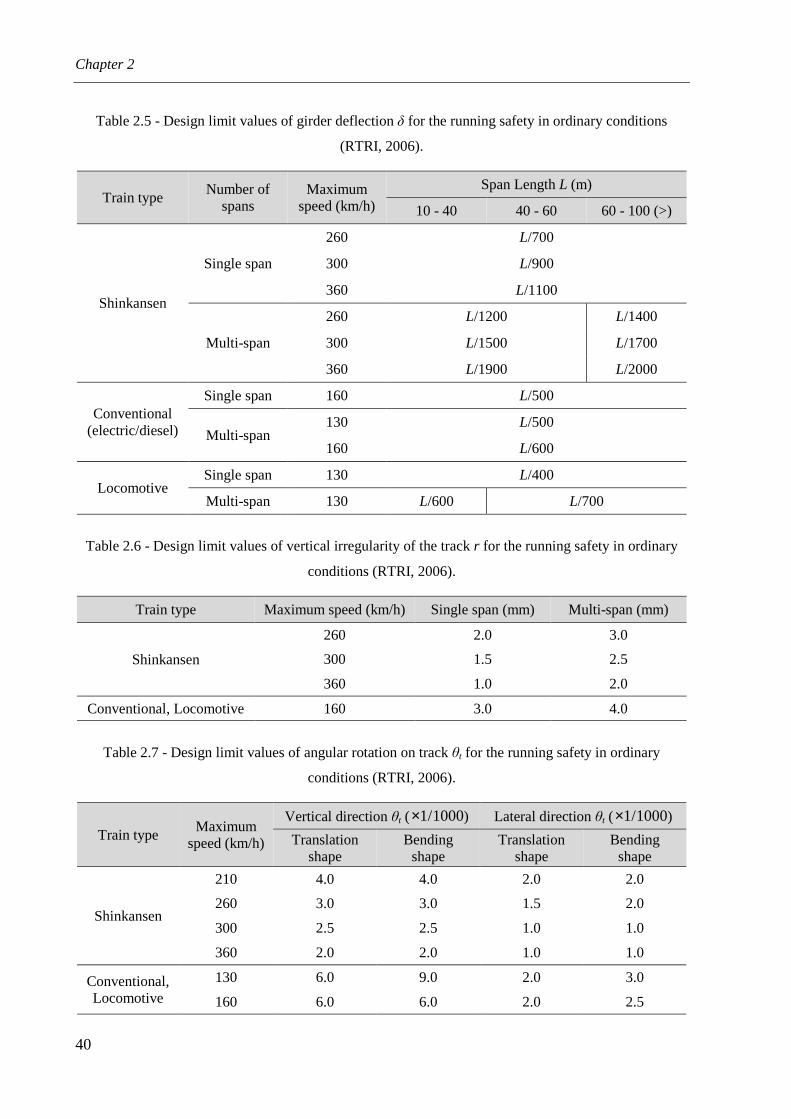
Chapter 2
40
Table 2.5 - Design limit values of girder deflection δ for the running safety in ordinary conditions
(RTRI, 2006).
Train type Number of
spans Maximum
speed (km/h)
Span Length L (m)
10 - 40 40 - 60 60 - 100 (>)
Shinkansen
Single span
260 L/700
300 L/900
360 L/1100
Multi-span
260 L/1200 L/1400
300 L/1500 L/1700
360 L/1900 L/2000
Conventional (electric/diesel)
Single span 160 L/500
Multi-span 130 L/500
160 L/600
Locomotive Single span 130 L/400
Multi-span 130 L/600 L/700
Table 2.6 - Design limit values of vertical irregularity of the track r for the running safety in ordinary
conditions (RTRI, 2006).
Train type Maximum speed (km/h) Single span (mm) Multi-span (mm)
Shinkansen
260 2.0 3.0
300 1.5 2.5
360 1.0 2.0
Conventional, Locomotive 160 3.0 4.0
Table 2.7 - Design limit values of angular rotation on track θt for the running safety in ordinary
conditions (RTRI, 2006).
Train type Maximum
speed (km/h)
Vertical direction θt ( 1000/1× ) Lateral direction θt ( 1000/1× )
Translation shape
Bending shape
Translation shape
Bending shape
Shinkansen
210 4.0 4.0 2.0 2.0
260 3.0 3.0 1.5 2.0
300 2.5 2.5 1.0 1.0
360 2.0 2.0 1.0 1.0
Conventional, Locomotive
130 6.0 9.0 2.0 3.0
160 6.0 6.0 2.0 2.5

State of the art
41
2.5.3.1.2 Displacements associated with the running safety in seismic conditions
The verification of the running safety in seismic condition aims to guarantee the adequate
performance of the structure in order to reduce the probability of derailment of a railway
vehicle during an earthquake. The running safety in seismic conditions is verified in terms of
the lateral vibration of the structure and in terms of the structural displacement indexes, namely
the lateral irregularity and the lateral angular rotations (see Figure 2.19).
Regarding the lateral vibration of the structure, the Displacement Limit Standard (RTRI,
2006) specifies design limit values for the vibration displacements caused by Level-1
earthquake motion2 (RTRI, 1999). The vibration displacements are evaluated based on a
concept of energy balance, called Spectral Intensity (SI) index, which reflects the amount of
energy of the seismic wave that influences the vehicle vibration (see Luo (2005) and Luo and
Miyamoto (2007) for more details about the SI index). The verification is performed by
computing the equivalent natural period of the structure Teq and checking if it falls in the safety
area given by the chart depicted in Figure 2.20 (the chart provides SI values for various types of
soils according to the Seismic Design Standard (RTRI, 1999)).
Figure 2.20 - Limit values of the SI index associated with the running safety in seismic conditions
(RTRI, 2006).
The design limit values for the structural displacement indexes, namely the lateral
irregularity and the lateral angular rotations, are given in Table 2.8. These limits cannot be
exceeded by the response of the structure when subjected to the Level-1 earthquake motion.
2 According to Seismic Design Standard (RTRI, 1999), Level-1 earthquake motion is prescribed based on the acceleration response spectrum determined for firm ground (bedrock), associated with a reference return period of 50 years and with a maximum spectral acceleration of 2.5 m/s2 (5% viscous damping).

Chapter 2
42
Table 2.8 - Design limit values of lateral angular rotations and irregularities for the running safety in
seismic conditions (RTRI, 2006).
Direction Maximum
speed (km/h)
Angular rotation θt ( 1000/1× ) Irregularity r
(mm) Translation shape Bending
shape L = 10 m L = 30 m
Lateral
130 7.0 7.0 8.0 14.0
160 6.0 6.0 6.0 12.0
210 5.5 3.5 4.0 10.0
260 5.0 3.0 3.5 8.0
300 4.5 2.5 3.0 7.0
360 4.0 2.0 2.0 6.0
2.5.3.2 Verification of restorability
The verification of restorability specifies two performance levels based on the amount of
damage of the track. They are the performance level 1, in which the track meets the necessary
requirements for a safe runnability and can be used without repairs, and performance level 2, in
which the normal functions of the track can be recovered in a short time but repair is necessary.
The verifications in both ordinary and seismic conditions aim to guarantee the performance
level 1 in order to ensure the safe stability of the track and, consequently, of the railway
vehicle.
Like in the safety verification reported in Section 2.5.3.1, the verification of restorability
may also be performed by developing a complex model of the entire structure, including the
track, using the stresses of each component of the track as the verification index, or by using
structural displacement indexes (see Figure 2.19). In practice, the second option is usually
adopted for simplicity, being the design limit values of the structural displacement indexes
defined in the Displacement Limit Standard (RTRI, 2006).
2.5.3.2.1 Restorability of track damage in ordinary conditions
The design limit values for the structural displacement indexes in ordinary conditions,
namely the irregularity of the track at the ends of the girder and the angular rotation on track
surfaces (see Figure 2.19) in both vertical and lateral directions are presented in Table 2.9. The
limits depend on the track type (slab track or ballast track) and on the type of rails used in
Japan (50kgN rail and 60kg rail).

State of the art
43
Table 2.9 - Design limit values of angular rotations and irregularities for the running safety in ordinary
conditions (RTRI, 2006).
Direction Track type
Angular rotation θt ( 1000/1× ) (Translation/bending shape)
Irregularity r (mm)
50kgN Rail
60kg Rail 50kgN Rail
60kg Rail Conventional Shinkansen
Vertical Slab 3.5 3.0 3.0
3.0 2.0 Ballast 6.0 5.5 7.0
Lateral Slab 4.0 4.0 4.0
2.0 2.0 Ballast 5.5 5.0 5.5
2.5.3.2.2 Restorability of track damage in seismic conditions
The design limit values for the structural displacement indexes in seismic conditions,
namely the irregularity of the track at the ends of the girder and the angular rotation on track
surfaces (see Figure 2.19) in both vertical and lateral directions are presented in Table 2.10.
This limits aim to guarantee the performance level 1 of restorability when the structure is
subjected to the Level 1 earthquake motion defined in the Seismic Design Standard (RTRI,
1999).
Table 2.10 - Design limit values of angular rotations and irregularities for the running safety in seismic
conditions (RTRI, 2006).
Direction Track type
Angular rotation θt ( 1000/1× ) (Translation/bending shape)
Irregularity r (mm)
50kgN Rail 60kg Rail 50kgN Rail 60kg Rail
Vertical Slab 5.0 3.5 4.5 3.5
Ballast 7.5 6.5 3.5 4.0
Lateral Slab 6.0 6.0 2.0 2.0
Ballast 8.0 8.0 2.0 2.0
2.5.4 North American standards
The running safety requirements adopted in the U.S.A., defined by the Manual of Standards
of the Association of American Railroads (AAR, 2011), are currently used only for freight
vehicles. However, a short description of the main requirements is presented, since most of
those requirements and criteria may also be used in the assessment of the running safety of
passenger trains.
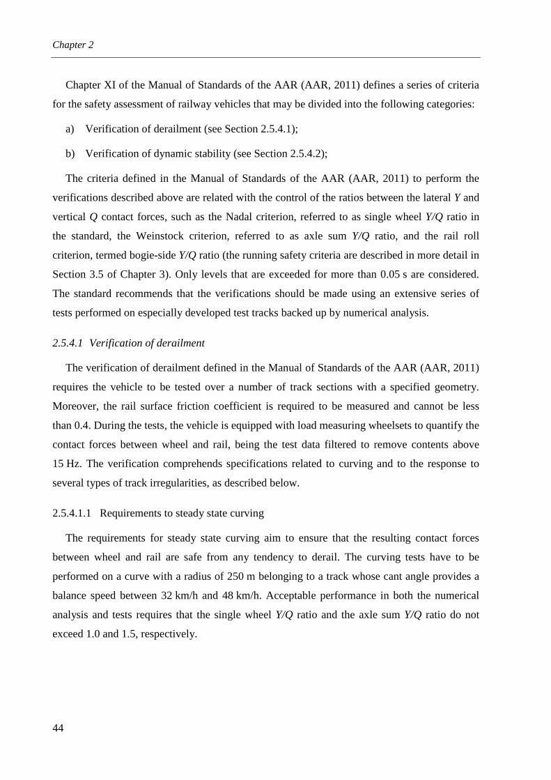
Chapter 2
44
Chapter XI of the Manual of Standards of the AAR (AAR, 2011) defines a series of criteria
for the safety assessment of railway vehicles that may be divided into the following categories:
a) Verification of derailment (see Section 2.5.4.1);
b) Verification of dynamic stability (see Section 2.5.4.2);
The criteria defined in the Manual of Standards of the AAR (AAR, 2011) to perform the
verifications described above are related with the control of the ratios between the lateral Y and
vertical Q contact forces, such as the Nadal criterion, referred to as single wheel Y/Q ratio in
the standard, the Weinstock criterion, referred to as axle sum Y/Q ratio, and the rail roll
criterion, termed bogie-side Y/Q ratio (the running safety criteria are described in more detail in
Section 3.5 of Chapter 3). Only levels that are exceeded for more than 0.05 s are considered.
The standard recommends that the verifications should be made using an extensive series of
tests performed on especially developed test tracks backed up by numerical analysis.
2.5.4.1 Verification of derailment
The verification of derailment defined in the Manual of Standards of the AAR (AAR, 2011)
requires the vehicle to be tested over a number of track sections with a specified geometry.
Moreover, the rail surface friction coefficient is required to be measured and cannot be less
than 0.4. During the tests, the vehicle is equipped with load measuring wheelsets to quantify the
contact forces between wheel and rail, being the test data filtered to remove contents above
15 Hz. The verification comprehends specifications related to curving and to the response to
several types of track irregularities, as described below.
2.5.4.1.1 Requirements to steady state curving
The requirements for steady state curving aim to ensure that the resulting contact forces
between wheel and rail are safe from any tendency to derail. The curving tests have to be
performed on a curve with a radius of 250 m belonging to a track whose cant angle provides a
balance speed between 32 km/h and 48 km/h. Acceptable performance in both the numerical
analysis and tests requires that the single wheel Y/Q ratio and the axle sum Y/Q ratio do not
exceed 1.0 and 1.5, respectively.
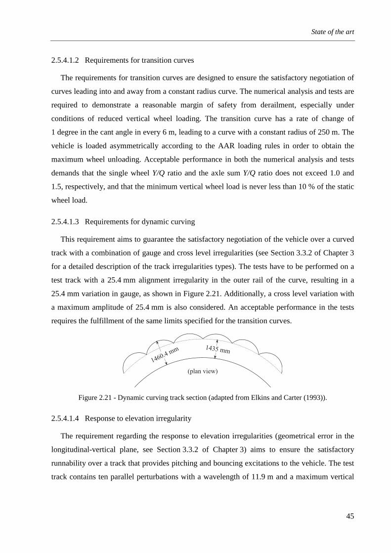
State of the art
45
2.5.4.1.2 Requirements for transition curves
The requirements for transition curves are designed to ensure the satisfactory negotiation of
curves leading into and away from a constant radius curve. The numerical analysis and tests are
required to demonstrate a reasonable margin of safety from derailment, especially under
conditions of reduced vertical wheel loading. The transition curve has a rate of change of
1 degree in the cant angle in every 6 m, leading to a curve with a constant radius of 250 m. The
vehicle is loaded asymmetrically according to the AAR loading rules in order to obtain the
maximum wheel unloading. Acceptable performance in both the numerical analysis and tests
demands that the single wheel Y/Q ratio and the axle sum Y/Q ratio does not exceed 1.0 and
1.5, respectively, and that the minimum vertical wheel load is never less than 10 % of the static
wheel load.
2.5.4.1.3 Requirements for dynamic curving
This requirement aims to guarantee the satisfactory negotiation of the vehicle over a curved
track with a combination of gauge and cross level irregularities (see Section 3.3.2 of Chapter 3
for a detailed description of the track irregularities types). The tests have to be performed on a
test track with a 25.4 mm alignment irregularity in the outer rail of the curve, resulting in a
25.4 mm variation in gauge, as shown in Figure 2.21. Additionally, a cross level variation with
a maximum amplitude of 25.4 mm is also considered. An acceptable performance in the tests
requires the fulfillment of the same limits specified for the transition curves.
Figure 2.21 - Dynamic curving track section (adapted from Elkins and Carter (1993)).
2.5.4.1.4 Response to elevation irregularity
The requirement regarding the response to elevation irregularities (geometrical error in the
longitudinal-vertical plane, see Section 3.3.2 of Chapter 3) aims to ensure the satisfactory
runnability over a track that provides pitching and bouncing excitations to the vehicle. The test
track contains ten parallel perturbations with a wavelength of 11.9 m and a maximum vertical
1435 mm
1460.4 mm
(plan view)
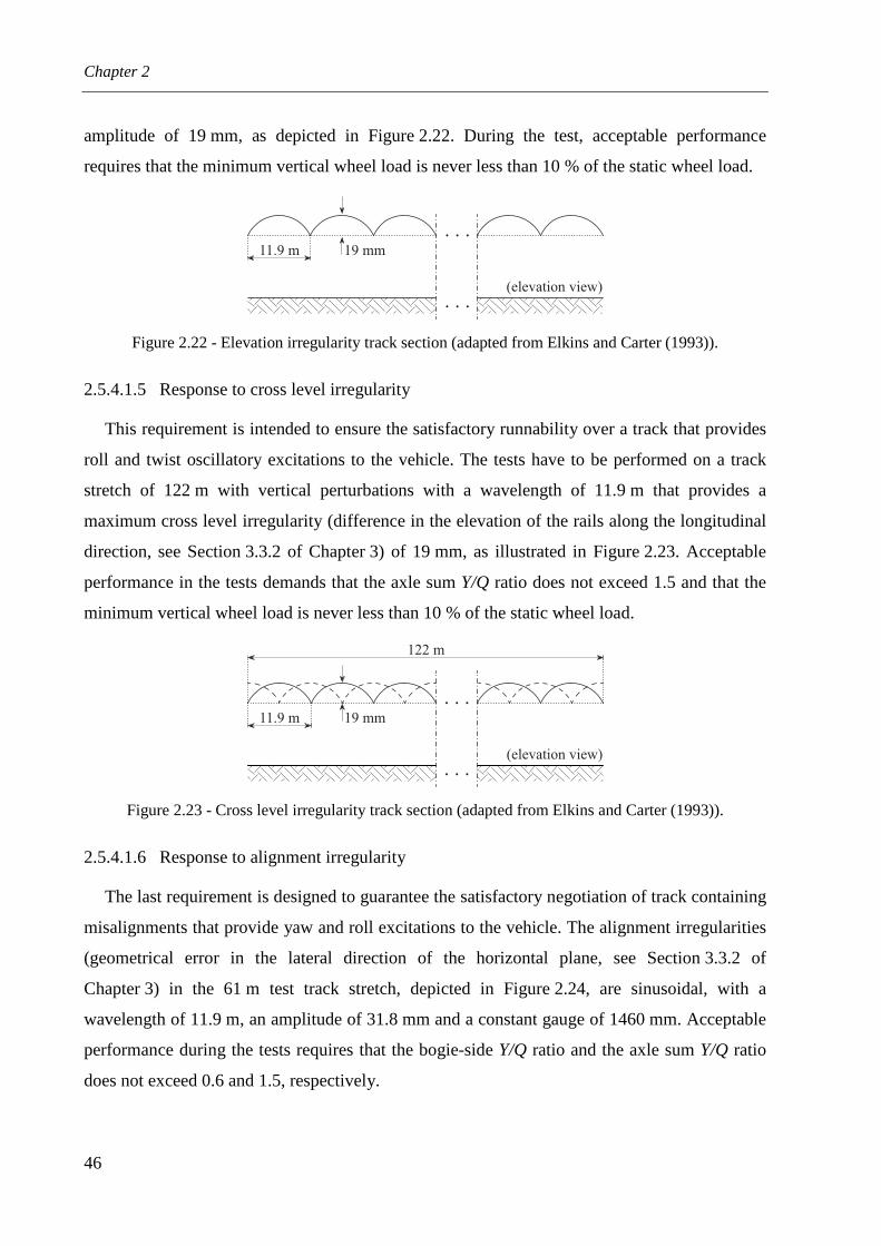
Chapter 2
46
amplitude of 19 mm, as depicted in Figure 2.22. During the test, acceptable performance
requires that the minimum vertical wheel load is never less than 10 % of the static wheel load.
Figure 2.22 - Elevation irregularity track section (adapted from Elkins and Carter (1993)).
2.5.4.1.5 Response to cross level irregularity
This requirement is intended to ensure the satisfactory runnability over a track that provides
roll and twist oscillatory excitations to the vehicle. The tests have to be performed on a track
stretch of 122 m with vertical perturbations with a wavelength of 11.9 m that provides a
maximum cross level irregularity (difference in the elevation of the rails along the longitudinal
direction, see Section 3.3.2 of Chapter 3) of 19 mm, as illustrated in Figure 2.23. Acceptable
performance in the tests demands that the axle sum Y/Q ratio does not exceed 1.5 and that the
minimum vertical wheel load is never less than 10 % of the static wheel load.
Figure 2.23 - Cross level irregularity track section (adapted from Elkins and Carter (1993)).
2.5.4.1.6 Response to alignment irregularity
The last requirement is designed to guarantee the satisfactory negotiation of track containing
misalignments that provide yaw and roll excitations to the vehicle. The alignment irregularities
(geometrical error in the lateral direction of the horizontal plane, see Section 3.3.2 of
Chapter 3) in the 61 m test track stretch, depicted in Figure 2.24, are sinusoidal, with a
wavelength of 11.9 m, an amplitude of 31.8 mm and a constant gauge of 1460 mm. Acceptable
performance during the tests requires that the bogie-side Y/Q ratio and the axle sum Y/Q ratio
does not exceed 0.6 and 1.5, respectively.
11.9 m 19 mm
. . .
. . . (elevation view)
11.9 m 19 mm
. . .
. . .
122 m
(elevation view)

State of the art
47
Figure 2.24 - Alignment irregularity track section (adapted from Elkins and Carter (1993)).
2.5.4.2 Verification of dynamic stability
According to the Manual of Standards of the AAR (AAR, 2011), the tests regarding the
verification of dynamic stability are performed to ensure the absence of lateral instability or
hunting within the operating speed of the vehicle. Numerical analyses are also performed to
predict the speed at which the lateral oscillations of the wheelset may lead to a continuous
flange-rail contact and to demonstrate that the magnitude of the wheel-rail contact forces and
the carbody lateral acceleration remain below the limit values. The limit values to guarantee an
acceptable performance regarding the dynamic stability of the vehicle consist of an unweighted
standard deviation of the carbody lateral acceleration of 2.6 m/s2 and an axle sum Y/Q ratio
of 1.5.
. . .
. . .
31.8 mm
61 m
11.9 m
14
60
(plan view)
mm


49
Chapter 3
FRAMEWORK OF THE METHODOLOGY FOR THE
ASSESSMENT OF THE TRAIN RUNNING SAFETY ON
BRIDGES
3.1 INTRODUCTION
In the present chapter, a methodology for assessing the train running safety on bridges is
presented (Montenegro et al., 2015a). Although the methodology may be applied to assess the
safety of trains subjected to several kinds of actions, such as, among others, earthquakes,
crosswinds or accident loads, the present work mainly focuses on the first. First, the proposed
methodology is introduced, along with a brief description of the background history of past
derailments caused by earthquakes. Then, the main source of excitations to the vehicle
considered in the present work, namely the earthquake and the track irregularities, are
described. Regarding the seismic action, since the running safety of the trains might be
jeopardized not only by intense shakings, but also by moderate earthquakes that do not cause
significant damage to the structure, only seismic events with relatively low return periods and
high probability of occurrence are considered in the present work. Therefore, no significant
nonlinearity is likely to be exhibited in the bridge piers for these levels of seismicity.
Nevertheless, the reduction in the stiffness of the piers due to concrete cracking is accounted
for, using a methodology developed by Montenegro et al. (2015a) and exposed in the third part
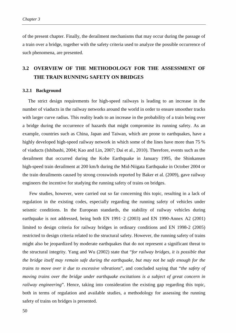
Chapter 3
50
of the present chapter. Finally, the derailment mechanisms that may occur during the passage of
a train over a bridge, together with the safety criteria used to analyze the possible occurrence of
such phenomena, are presented.
3.2 OVERVIEW OF THE METHODOLOGY FOR THE ASSESSMENT OF
THE TRAIN RUNNING SAFETY ON BRIDGES
3.2.1 Background
The strict design requirements for high-speed railways is leading to an increase in the
number of viaducts in the railway networks around the world in order to ensure smoother tracks
with larger curve radius. This reality leads to an increase in the probability of a train being over
a bridge during the occurrence of hazards that might compromise its running safety. As an
example, countries such as China, Japan and Taiwan, which are prone to earthquakes, have a
highly developed high-speed railway network in which some of the lines have more than 75 %
of viaducts (Ishibashi, 2004; Kao and Lin, 2007; Dai et al., 2010). Therefore, events such as the
derailment that occurred during the Kobe Earthquake in January 1995, the Shinkansen
high-speed train derailment at 200 km/h during the Mid-Niigata Earthquake in October 2004 or
the train derailments caused by strong crosswinds reported by Baker et al. (2009), gave railway
engineers the incentive for studying the running safety of trains on bridges.
Few studies, however, were carried out so far concerning this topic, resulting in a lack of
regulation in the existing codes, especially regarding the running safety of vehicles under
seismic conditions. In the European standards, the stability of railway vehicles during
earthquake is not addressed, being both EN 1991‑2 (2003) and EN 1990-Annex A2 (2001)
limited to design criteria for railway bridges in ordinary conditions and EN 1998-2 (2005)
restricted to design criteria related to the structural safety. However, the running safety of trains
might also be jeopardized by moderate earthquakes that do not represent a significant threat to
the structural integrity. Yang and Wu (2002) state that “for railway bridges, it is possible that
the bridge itself may remain safe during the earthquake, but may not be safe enough for the
trains to move over it due to excessive vibrations”, and concluded saying that “the safety of
moving trains over the bridge under earthquake excitations is a subject of great concern in
railway engineering”. Hence, taking into consideration the existing gap regarding this topic,
both in terms of regulation and available studies, a methodology for assessing the running
safety of trains on bridges is presented.

Framework of the methodology for the assessment of the train running safety on bridges
51
3.2.2 Description of the methodology
Figure 3.1 illustrates the framework of the proposed methodology for the assessment of the
train running safety on bridges. The methodology consists of calculating the wheel-rail contact
forces during the passage of the train over the bridge in order to evaluate the risk of derailment
through existing running safety criteria. The dynamic analyses are performed with the
train-structure interaction method developed by Montenegro et al. (2015b) and described later
in Chapter 4.
Figure 3.1 - Framework of the methodology for the assessment of the train running safety on bridges.
Although the methodology is generalized to allow the safety assessment of trains under any
kind of conditions, as shown in Figure 3.1, the present work focuses mainly on the running
safety against earthquakes. Thus, the seismic motion is represented in terms of ground
acceleration time-histories using artificial accelerograms (Section 3.3.1) that are generated from
the elastic spectra described in EN 1998-1 (2004), with peak ground accelerations (PGA)
win
d l
oad
therm
al load
Conta
ct
forc
e
Time
Viaduct
with wheel-rail contact(Chapters 4 and 5)
Seismic behavior of the piers
Track irregularities
(Section 3.3.2 - Chapter 3)
Seismic action
Wheel-rail contact forces(Chapter 4)
Running safety criteria
Safe Unsafe
Prud'hommeNadal
Wheel unload
(Section 3.4 - Chapter 3)
(Section 3.3.1 - Chapter 3)
(Section 3.5 - Chapter 3)
rV
rC
Fn
Adh.Slip
τσ
Fη,ξ
δ
Fb
Fb
δ
gaɺɺ
Rail rollover
Other actions
(Section 3.3.3 - Chapter 3)
Train-structure interaction
Y
QY

Chapter 3
52
corresponding to moderate events with relatively high probability of occurrence and low return
periods. Since no significant nonlinearity is likely to be exhibited in the bridge piers for these
levels of seismicity, all the analysis are performed in the elastic domain with a reduction in the
stiffness of the piers to account for concrete cracking. The reduced stiffness, referred to as
effective stiffness, is calculated based on the methodology developed by Montenegro et al.
(2015a) and described in Section 3.4. This methodology is divided into three main steps, which
consist of:
a) Nonlinear static analysis to assess the horizontal monotonic behavior of the piers;
b) Nonlinear dynamic analysis to evaluate the maximum response at the top of the pier;
c) Calibration of the effective stiffness based on the two aforementioned analyses.
Track irregularities, which consist of deviations of the rail from its ideal geometry, are also
an important source of excitation for the vehicle. In the present work, the irregularity profiles
are generated based on analytical power spectral density (PSD) functions (Section 3.3.2).
Finally, the running safety of the train is evaluated using safety criteria based on the
wheel-rail contact forces that are recommended by the several codes reported in Section 2.5 of
Chapter 2, such as Nadal (1908), Prud'homme (1967), rail rollover (AAR, 2011) and wheel
unloading (EN 14067-6, 2010) criteria (Section 3.5). Therefore, for each scenario, the
circulation is considered to be safe as long as none of the safety criteria is violated during the
whole time the vehicle is crossing the bridge.
3.3 SOURCES OF EXCITATION OF THE TRAIN-STRUCTURE SYSTEM
3.3.1 Seismic action
3.3.1.1 Representation of the seismic action
The seismic excitations adopted in the present work consist of artificial accelerograms
generated from the elastic spectra described in EN 1998-1 (2004), with PGA corresponding to
moderate events with return periods less than 475 years, which is the reference return period of
the design seismic action associated with the no-collapse requirement. This type of seismic
actions is of the utmost importance, since the running safety of trains might be jeopardized not
only by intense earthquakes, but also by moderate seismic events, which may not cause
significant damage to the structure. Figure 3.2 illustrates an example of one of the generated

Framework of the methodology for the assessment of the train running safety on bridges
53
accelerograms (return period equal to 310 years), as well as the respective response spectrum
adjustment to the target spectrum given by EN 1998-1 (2004).
(a) (b)
Figure 3.2 - Example of a generated ground motion: (a) accelerogram and (b) spectrum adjustment.
3.3.1.2 Generation of artificial accelerograms
The artificial accelerograms are generated with the software SeismoArtif (2013), which uses
a method based on a random process of adjustment by correction in the frequency domain. This
method defines the artificial ground motion considering a target spectrum and adapting the
frequency content through an iterative process using the Fourier Transformation Method.
The ground motion ( )tagɺɺ is generated based on the fact that each periodic function can be
expressed as a series of sinusoidal waves, and is defined as (Gasparini and Vanmarcke, 1976)
( ) ( ) ( )nnn
ng tAtIta φω += ∑ sinɺɺ (3.1)
where An, nω and nφ are the amplitude, frequency and phase angle, respectively, of the nth
sinusoidal wave considered, and ( )tI an intensity function to simulate the transient nature of
the earthquake. By defining a vector of amplitudes and simulating different arrays with a
random set of phase angles, it is possible to obtain different processes with the same general
aspect but with different characteristics. These random processes are stationary and their
characteristics do not change with time. In the present method, the random phase angles nφ are
uniformly distributed in the range [ ]π2,0 .
0 2 4 6 8 10 12 14−1.5
−1.0
−0.5
0.0
0.5
1.0
1.5
Time (s)
Ground acceleration (m.s−2)
0 1 2 3 40.0
1.0
2.0
3.0
4.0
Period (s)
Sp
ectr
al a
ccel
erat
ion (
m.s
−2) Target spectrum EC8
Target spectrum EC8 + 10%Target spectrum EC8 − 10%Generated spectrum

Chapter 3
54
The method used by SeismoArtif to generate the artificial accelerograms comprehends an
iterative process. Therefore, for each cycle, the response spectrum generated for the simulated
ground motion is compared with the target spectrum at a set of control frequencies, being the
correction of the random process performed in the frequency domain. Figure 3.3 outlines the
main steps of the artificial accelerogram generation process.
Figure 3.3 - Schematization of the generation process of artificial accelerograms (SeismoArtif, 2013).
3.3.2 Track irregularities
3.3.2.1 Types of track irregularities
Track irregularities are an important source of excitation for both the structure and the
vehicle. The irregularities are deviations of the track from the design geometry (see Figure 3.4)
that can be divided into the following four types (Frýba, 1996; Andersson et al., 1999):
a) Elevation level: geometrical error in the longitudinal-vertical plane;
b) Alignment: geometrical error in the lateral direction of the horizontal plane;
c) Cross level: difference in the elevation of the rails along the longitudinal direction;
d) Gauge: variation in the track gauge.
Figure 3.4 - Types of track irregularities: (a) perspective view; (b) elevation view and (c) plan view.
Elevation
Cross level Alignment
Gauge
y
x z
z
x y
level
Left rail
Right rail
Left rail
Right rail z
x yLeft rail
Right rail
(a) (b) (c)

Framework of the methodology for the assessment of the train running safety on bridges
55
Therefore, considering yr and zr as the lateral and vertical deviations, respectively, the
elevation Vr , alignment Ar , cross level Cr and gauge Gr irregularities can be defined as
function of the longitudinal coordinate x as following:
( ) ( )lftz
rhtzV rrxr +=
2
1 (3.2a)
( ) ( )lfty
rhtyA rrxr +=
2
1 (3.2b)
( ) lftz
rhtzC rrxr −= (3.2c)
( ) lfty
rhtyG rrxr −= (3.2d)
where the superscripts lft and rht indicate left and right rails, respectively.
3.3.2.2 Power spectral density functions
In order to account for the track irregularities in the train-structure interaction analysis, it is
necessary to analytically describe the track geometry. However, since it is usually difficult to
have access to a detailed description of the track, the irregularities are commonly defined as a
stationary stochastic process that may be described by PSD functions.
Each of the aforementioned irregularity profiles r can be understood as a stochastic Gaussian
ergodic process that is characterized by the mean value r given by (Claus and Schiehlen,
1998)
( )∫∞→=
L
Ldxxr
Lr
0
1lim (3.3)
and by the correlation function Rr that can be written as
( ) ( ) ( )∫ −=∞→
L
Lr dxxrxr
LR
0
1lim ζζ (3.4)
The Fourier transform of the correlation function results in the PSD function S, which can be
defined as
( ) ( ) ζζ ζ deRS jr
Ω−+∞
∞−∫=Ω (3.5)
where Ω is the spatial frequency.

Chapter 3
56
According to Claus and Schiehlen (1998), various measurements of track irregularities have
shown that the PSD can be standardized and expressed as
( ) ( ) ( )2222
2
,, 2
1
Ω+ΩΩ+ΩΩ=Ω
cr
cVAVA AS (3.6a)
( ) ( ) ( ) ( )222222
22
,2,
1
Ω+ΩΩ+ΩΩ+ΩΩΩ=Ω
scr
cCGCG A
lS (3.6b)
where the subscripts A, V, G and C indicate the alignment, elevation level, gauge and cross
level irregularities, l is half of the gauge, A is the irregularity scale factor, and cΩ , rΩ and
sΩ are constant factors. According to Claus and Schiehlen (1998), the values of these constant
factors, which are representative of the European railway network, are
mrad8246.0=Ωc (3.7a)
mrad0206.0=Ωr (3.7b)
mrad4380.0=Ωs (3.7c)
The PSD functions of the elevation irregularity for three distinct levels of track quality are
represented, for exemplification purposes, in Figure 3.5. The three PSD functions refer to the
low, medium and high levels of irregularities described by Claus and Schiehlen (1998),
represented by scale factors of m.rad1059233.0 6−×=lowA , m.rad1008922.1 6−×=mediumA and
m.rad1058610.1 6−×=highA , respectively.
Figure 3.5 - PSD functions of the alignment irregularity for three distinct levels of track quality.
0.0 0.5 1.0 1.50
2
4
6
8
10Low level
Medium level
High level
()
3m
rad
vS
x10−5
( )rad mΩ
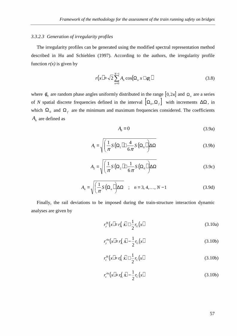
Framework of the methodology for the assessment of the train running safety on bridges
57
3.3.2.3 Generation of irregularity profiles
The irregularity profiles can be generated using the modified spectral representation method
described in Hu and Schiehlen (1997). According to the authors, the irregularity profile
function r(x) is given by
( ) ( )nn
N
nn xAxr φ+Ω= ∑
−
=
cos21
0
(3.8)
where nφ are random phase angles uniformly distributed in the range [ ]π2,0 and nΩ are a series
of N spatial discrete frequencies defined in the interval [ ]fΩΩ ,0 with increments ∆Ω , in
which 0Ω and fΩ are the minimum and maximum frequencies considered. The coefficients
nA are defined as
00 =A (3.9a)
( ) ( ) ∆Ω
Ω+Ω= 011 6
41SSA
ππ (3.9b)
( ) ( ) ∆Ω
Ω+Ω= 022 6
11SSA
ππ (3.9c)
( ) 1,,4,3;1 −=∆Ω
Ω= NnSA nn …π
(3.9d)
Finally, the rail deviations to be imposed during the train-structure interaction dynamic
analyses are given by
( ) ( ) ( )xrxrxr GAlfty 2
1+= (3.10a)
( ) ( ) ( )xrxrxr GArhty 2
1−= (3.10b)
( ) ( ) ( )xrxrxr CVlftz 2
1+= (3.10b)
( ) ( ) ( )xrxrxr CVrhtz 2
1−= (3.10b)
Chapter 3
58
3.3.3 Other sources of excitation
Although the present work is only focused on the running safety of trains under seismic
conditions, the methodology proposed in the present chapter is capable of dealing with any
other type of external loads that may influence the running stability of the railway vehicle.
Therefore, static or dynamic wind loads (Section 8 of EN 1991-1-4 (2005) and EN 14067-6
(2010)), applied both to the structure and vehicle, accident loads due to impact on supporting
members of the structure caused by derailed trains passing under or adjacent to structures
(Section 4.5 of EN 1991-1-7 (2006)) or thermal loads that may cause the rails to buckle
(UIC 774-3-R, 2001), are all actions that can put the stability of the vehicle at risk as well and
that may also be considered in the model.
3.4 MODELING OF THE SEISMIC BEHAVIOR OF THE BRIDGE PIER S
3.4.1 Introduction
According to EN 1998-2 (2005), when an equivalent linear analysis is used, the effective
flexural stiffness of a reinforced concrete member should correspond to the secant stiffness at
the theoretical yield point. However, the present study focus on the train running safety on
bridges during moderate earthquakes in which, in general, the piers do not experience
significant damage and the yield point is not reached. Thus, an alternative methodology to
estimate the effective stiffness of the bridge piers to be used in the train-structure interaction
analyses performed in the elastic domain is presented. The methodology is divided in the
following steps: 1) a nonlinear static analysis to evaluate the horizontal monotonic behavior of
the piers; 2) a nonlinear dynamic analysis to determine the maximum displacement at the top of
the pier when subjected to the seismic excitations and 3) calibration of the effective stiffness in
order to obtain, with a linear dynamic analysis, levels of displacement similar to those obtained
with the nonlinear dynamic analysis. These three steps are described in detail in Sections 3.4.2
through 3.4.4.
3.4.2 Monotonic response of the bridge piers
The first step of the methodology consists of performing a nonlinear monotonic static
analysis to evaluate the horizontal response of the piers, as depicted in Figure 3.6. In this type
of analysis, the idealized representation of the structure is subjected to a constant gravity load
Fw and to a monotonically increasing force or displacement δ at the pier top that represent the

Framework of the methodology for the assessment of the train running safety on bridges
59
inertial effects from the earthquake (Elnashai and Sarno, 2008). Since the forcing function is
increased until the ultimate capacity of the pier is reached, the structure model has to account
for the effects of both the material inelasticity and the geometric nonlinearity. Thus, to perform
this type of analysis, the piers are commonly modeled using frame elements with distributed
inelasticity based on the displacement-based formulation, in which the sectional stress-strain
state is obtained through the integration of the nonlinear uniaxial material response of the
individual fibers used to discretize the cross-section.
The results obtained with the monotonic analysis are expressed in terms of a capacity curve
(see Figure 3.6), which consists in the relation between the global base shear force Fb and the
displacement δ at the top of the pier. In the present work, the nonlinear monotonic static
analysis is performed using the software SeismoStruct (2013) .
Figure 3.6 - Nonlinear monotonic static analysis.
3.4.3 Nonlinear dynamic analysis
The second step of the methodology consists of performing a nonlinear dynamic analysis to
predict the inelastic response of the piers subjected to the seismic excitation. The structure,
whose model also have to account for the effects of material and geometric nonlinearities, is
subjected to the seismic ground motion gaɺɺ applied at the base of the piers, as depicted in
Figure 3.7. Then, the maximum displacement at the top of the pier δmax is computed. This
value, together with the horizontal capacity of the piers obtained in the monotonic analysis
deck CG
pier model
pier top
wF
bF
δ
Plastification
Displacement δ
Bas
e sh
ear
bF
Cracking
Capacity curve of the pier

Chapter 3
60
presented in the previous section, is used to calibrate the effective stiffness of the piers, as
shown in Section 3.4.4.
Due to the dynamic nature of the analysis, damping has to be accounted for in order to
obtain a realistic result. The hysteretic component of damping, which is usually responsible for
the dissipation of the majority of the energy introduced by the earthquake load, is already
included within the elements with nonlinear behavior. However, since the proposed
methodology focuses on the analysis of the seismic behavior of piers that do not experience
significant levels of plasticity, the non-hysteretical damping that is mobilized during the
dynamic response of the structure, through phenomena such as friction and energy radiation,
also plays an important role. Therefore, this energy dissipation mechanism is accounted by
means of Rayleigh damping (Clough and Penzien, 2003), with an equivalent viscous damping
ratio fixed in the frequencies of the pier obtained using the elastic stiffness of an uncracked
cross-section and using the effective stiffness estimated with the Annex C of EN 1998-2 (2005)
for reinforced concrete ductile members. This criterion is based on the fact that the natural
frequency of the piers after the calibration of the effective flexural stiffness is somewhere
between the two aforementioned frequencies. The nonlinear dynamic analysis is also performed
using the software SeismoStruct.
Figure 3.7 - Nonlinear dynamic analysis.
pier model
deck GC
pier top
gaɺɺ
maxδ
Dis
pla
cem
ent
Time
maxδ
Response at the top of the pier

Framework of the methodology for the assessment of the train running safety on bridges
61
3.4.4 Calibration of the effective stiffness of the bridge piers
The final step of the present methodology consists of calibrating the effective stiffness of the
piers in order to obtain, with a linear dynamic analysis, levels of displacement similar to those
obtained with the nonlinear dynamic analysis presented in the previous section. Thus, the base
shear force Fb, obtained in the capacity curve (see Section 3.4.2), corresponding to the
maximum displacement at the top of the pier δmax computed in the nonlinear dynamic analysis
(see Section 3.4.3) is evaluated, as depicted in Figure 3.8. The effective flexural stiffness of the
pier will correspond to the secant stiffness at the aforementioned point. The stiffness is
calculated numerically or, in the case of simple structures whose flexural stiffness can be
approximated by a closed-form expression, analytically.
Figure 3.8 - Base shear force Fb corresponding to the maximum displacement δmax at the top of the pier.
3.5 DERAILMENT MECHANISMS AND SAFETY CRITERIA
The assessment of the running safety of trains is a topic of the utmost importance in railway
engineering. Therefore, it is important to ensure that the criteria used to evaluate the safety of
vehicles are realistic enough to avoid the occurrence of derailments. Train derailments are the
result of wheels running off the rails that provide the necessary guidance to the vehicle. The
reasons for wheels running off the rail can be difficult to ascertain. However, the final scenario
of derailment may result in wheels climbing off the rail, gauge widening or rail rollover,
causing the wheels to fall between the rails (Wu and Wilson, 2006). Hence, any situation that
may reduce the lateral guidance provided by the rails will surely increase the risk of derailment.
Plastic region
Effective stiffness
Displacement
Elastic stiffness
Bas
e sh
ear
maxδ
bF (not reached with the
considered seismic intensities)
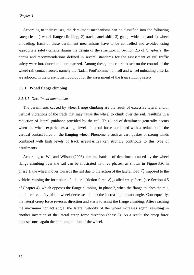
Chapter 3
62
According to their causes, the derailment mechanisms can be classified into the following
categories: 1) wheel flange climbing; 2) track panel shift; 3) gauge widening and 4) wheel
unloading. Each of these derailment mechanisms have to be controlled and avoided using
appropriate safety criteria during the design of the structure. In Section 2.5 of Chapter 2, the
norms and recommendations defined in several standards for the assessment of rail traffic
safety were introduced and summarized. Among these, the criteria based on the control of the
wheel-rail contact forces, namely the Nadal, Prud'homme, rail roll and wheel unloading criteria,
are adopted in the present methodology for the assessment of the train running safety.
3.5.1 Wheel flange climbing
3.5.1.1 Derailment mechanism
The derailments caused by wheel flange climbing are the result of excessive lateral and/or
vertical vibrations of the track that may cause the wheel to climb over the rail, resulting in a
reduction of lateral guidance provided by the rail. This kind of derailment generally occurs
when the wheel experiences a high level of lateral force combined with a reduction in the
vertical contact force on the flanging wheel. Phenomena such as earthquakes or strong winds
combined with high levels of track irregularities can strongly contribute to this type of
derailments.
According to Wu and Wilson (2006), the mechanism of derailment caused by the wheel
flange climbing over the rail can be illustrated in three phases, as shown in Figure 3.9. In
phase 1, the wheel moves towards the rail due to the action of the lateral load lF imposed to the
vehicle, causing the formation of a lateral friction force ηF , called creep force (see Section 4.5
of Chapter 4), which opposes the flange climbing. In phase 2, when the flange touches the rail,
the lateral velocity of the wheel decreases due to the increasing contact angle. Consequently,
the lateral creep force reverses direction and starts to assist the flange climbing. After reaching
the maximum contact angle, the lateral velocity of the wheel increases again, resulting in
another inversion of the lateral creep force direction (phase 3). As a result, the creep force
opposes once again the climbing motion of the wheel.

Framework of the methodology for the assessment of the train running safety on bridges
63
Figure 3.9 - Mechanism of derailment caused by wheel flange climbing: (a) phase 1, (b) phase 2 and
(c) phase 3.
3.5.1.2 Nadal criterion
One of the most common criterion used to assess the derailment caused by wheel flange
climbing was proposed by Nadal (1908) in the beginning of the 20th century. This criterion
limits the ratio between the lateral Y and vertical Q contact force in each wheel, commonly
known as derailment index or derailment coefficient, in order to minimize the risk of
derailment. Based on a simple equilibrium of forces between the wheel and rail at a single
contact point in the flange, as depicted in Figure 3.10, the Y/Q ratio, referred to in this work as
the Nadal factor Nζ , can be expressed as
γ
γζ
η
η
tan1
tan
n
nN
F
FF
F
Q
Y
+
−== (3.11)
where γ is the contact angle between the wheel and rail, nF the normal contact force and ηF
the lateral creep force. Nadal proposed the criterion for the saturation condition, leading to
γµ
µγζtan1
tan
+−==
Q
YN (3.12)
where µ is the friction coefficient. The limit value for the Y/Q ratio varies from country to
country, depending on the friction coefficient considered and on the wheel flange inclinations.
According to TSI (2002), the Y/Q ratio in any wheel of the train should not exceed 0.8. The
same limit is imposed in Japan (RTRI, 2006), while in the U.S.A. and China the Y/Q ratio is
allowed to reach 1.0 (AAR, 2011 and Jun and Qingyuan (2005)).
(a) (b) (c)
lF lF lF
Fη Fη
Fη
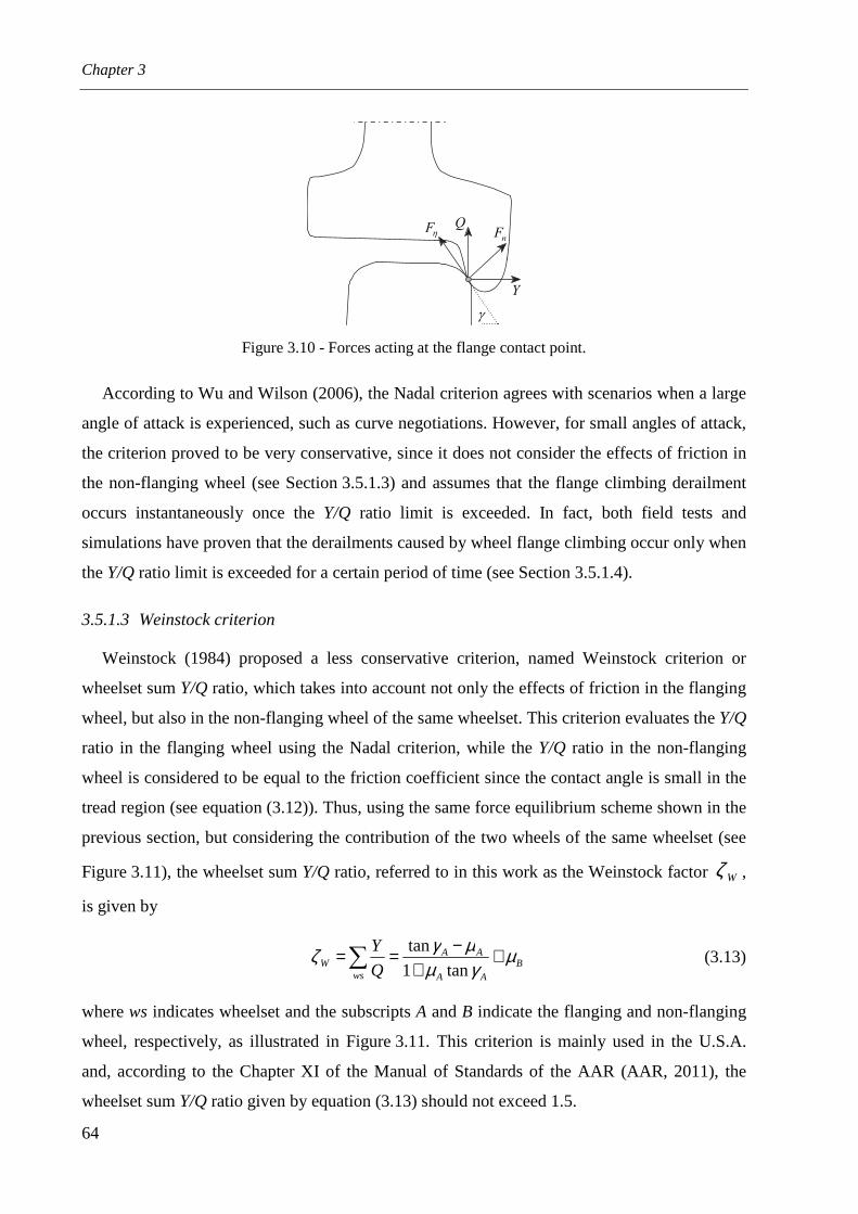
Chapter 3
64
Figure 3.10 - Forces acting at the flange contact point.
According to Wu and Wilson (2006), the Nadal criterion agrees with scenarios when a large
angle of attack is experienced, such as curve negotiations. However, for small angles of attack,
the criterion proved to be very conservative, since it does not consider the effects of friction in
the non-flanging wheel (see Section 3.5.1.3) and assumes that the flange climbing derailment
occurs instantaneously once the Y/Q ratio limit is exceeded. In fact, both field tests and
simulations have proven that the derailments caused by wheel flange climbing occur only when
the Y/Q ratio limit is exceeded for a certain period of time (see Section 3.5.1.4).
3.5.1.3 Weinstock criterion
Weinstock (1984) proposed a less conservative criterion, named Weinstock criterion or
wheelset sum Y/Q ratio, which takes into account not only the effects of friction in the flanging
wheel, but also in the non-flanging wheel of the same wheelset. This criterion evaluates the Y/Q
ratio in the flanging wheel using the Nadal criterion, while the Y/Q ratio in the non-flanging
wheel is considered to be equal to the friction coefficient since the contact angle is small in the
tread region (see equation (3.12)). Thus, using the same force equilibrium scheme shown in the
previous section, but considering the contribution of the two wheels of the same wheelset (see
Figure 3.11), the wheelset sum Y/Q ratio, referred to in this work as the Weinstock factor Wζ ,
is given by
BAA
AA
wsW Q
Y µγµ
µγζ ++
−==∑ tan1
tan (3.13)
where ws indicates wheelset and the subscripts A and B indicate the flanging and non-flanging
wheel, respectively, as illustrated in Figure 3.11. This criterion is mainly used in the U.S.A.
and, according to the Chapter XI of the Manual of Standards of the AAR (AAR, 2011), the
wheelset sum Y/Q ratio given by equation (3.13) should not exceed 1.5.
Y
QFηnF
γ
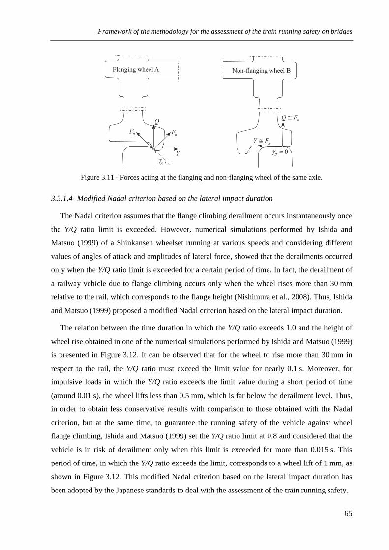
Framework of the methodology for the assessment of the train running safety on bridges
65
Figure 3.11 - Forces acting at the flanging and non-flanging wheel of the same axle.
3.5.1.4 Modified Nadal criterion based on the lateral impact duration
The Nadal criterion assumes that the flange climbing derailment occurs instantaneously once
the Y/Q ratio limit is exceeded. However, numerical simulations performed by Ishida and
Matsuo (1999) of a Shinkansen wheelset running at various speeds and considering different
values of angles of attack and amplitudes of lateral force, showed that the derailments occurred
only when the Y/Q ratio limit is exceeded for a certain period of time. In fact, the derailment of
a railway vehicle due to flange climbing occurs only when the wheel rises more than 30 mm
relative to the rail, which corresponds to the flange height (Nishimura et al., 2008). Thus, Ishida
and Matsuo (1999) proposed a modified Nadal criterion based on the lateral impact duration.
The relation between the time duration in which the Y/Q ratio exceeds 1.0 and the height of
wheel rise obtained in one of the numerical simulations performed by Ishida and Matsuo (1999)
is presented in Figure 3.12. It can be observed that for the wheel to rise more than 30 mm in
respect to the rail, the Y/Q ratio must exceed the limit value for nearly 0.1 s. Moreover, for
impulsive loads in which the Y/Q ratio exceeds the limit value during a short period of time
(around 0.01 s), the wheel lifts less than 0.5 mm, which is far below the derailment level. Thus,
in order to obtain less conservative results with comparison to those obtained with the Nadal
criterion, but at the same time, to guarantee the running safety of the vehicle against wheel
flange climbing, Ishida and Matsuo (1999) set the Y/Q ratio limit at 0.8 and considered that the
vehicle is in risk of derailment only when this limit is exceeded for more than 0.015 s. This
period of time, in which the Y/Q ratio exceeds the limit, corresponds to a wheel lift of 1 mm, as
shown in Figure 3.12. This modified Nadal criterion based on the lateral impact duration has
been adopted by the Japanese standards to deal with the assessment of the train running safety.
Flanging wheel A
Y
Q
Fη nF
Y Fη≅
nQ F≅
0Bγ ≃
Aγ
Non-flanging wheel B

Chapter 3
66
Figure 3.12 - Time duration of the Y/Q ratio versus the height of wheel rise obtained in the simulation of
a Shinkansen wheelset running at different speeds (adapted from Ishida and Matsuo, 1999).
3.5.2 Track panel shift
3.5.2.1 Derailment mechanism
The track panel shift is the lateral displacement of the track panel, which includes the rails
and the sleepers, over the ballast, as shown in Figure 3.13. As the cumulative lateral
displacement of the track panel over the ballast increases, the wheels may lose guidance,
resulting in one wheel falling between the rails and the other outside the track. This
phenomenon is mainly caused by repeated lateral axle loads applied to the rails, and is
associated with tracks that possess low lateral resistance, such as poorly laid tracks, newly laid
tracks and newly maintained tracks, or with tracks laid over soft subgrades.
According to Elkins and Carter (1993) and Wu and Wilson (2006), the track panel shift
phenomenon has become increasingly important with the increase of train speeds and loads. In
fact, the increase in speed generally results in an increase in the unbalanced forces on curves or
on poorly aligned tracks. These unbalanced forces act to force the rail outwards in a curve,
resulting in panel shift and, consequently, leading to a higher risk of derailment. Moreover, the
greater use of continuously welded rail also contributes for increasing the probability of panel
shift due to the buckling phenomenon caused by temperature changes in the rails.
Hei
ght
of
whee
l ri
se (
mm
)
100
50
10
5
1
0.5
0.10.001 0.01 0.1 0.5
Time duration of Y/Q (s)
Wheel rise = 30 mm
1t.
d. =
0.0
15 s
: 300km/h
: 400km/h
: 500km/h
Framework of the methodology for the assessment of the train running safety on bridges
67
Figure 3.13 - Mechanism of derailment caused by track panel shift.
3.5.2.2 Prud'homme criterion
Research performed by the French National Railways Company (Sonneville and Bentot,
1955) suggested that the lateral load induced by a single wheelset should be limited to prevent
excessive track panel shift. Subsequent research reported by Prud'homme (1967) specified the
following criterion for limiting the total lateral force Y exerted by a wheelset on the track :
[ ]kN3
210 0Q
Yws
+=∑ (3.14)
where Q0 is the static load per wheel in kilonewtons. The criterion is adopted in Europe by the
TSI (2002). In this work, the Prud'homme factor Pζ is expressed in a dimensionless form as
[ ]
[ ]kN3
210
kN
0Q
Yws
P
+=
∑ζ (3.15)
3.5.3 Gauge widening caused by rail rollover
3.5.3.1 Derailment mechanism
A derailment caused by gauge widening usually involves the combination of wide gauges
and large rail lateral deflections, mainly due to the rail rollover. The rail rollover is a result of
important impacts between wheel and rail that occur when the wheelsets experience high
angles of attack due to the poor steering of the bogie. These impacts lead to large lateral forces
exerted on the rails that may deflect them further. This type of derailment may occur when the
gauge faces of the two rails are spread enough to allow one of the wheels to drop between the
rails, as illustrated in Figure 3.14.
Panel shift Panel movement
direction
SleeperBallast layer
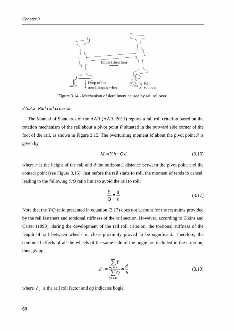
Chapter 3
68
Figure 3.14 - Mechanism of derailment caused by rail rollover.
3.5.3.2 Rail roll criterion
The Manual of Standards of the AAR (AAR, 2011) reports a rail roll criterion based on the
rotation mechanism of the rail about a pivot point P situated in the outward side corner of the
foot of the rail, as shown in Figure 3.15. The overturning moment M about the pivot point P is
given by
dQhYM −= (3.16)
where h is the height of the rail and d the horizontal distance between the pivot point and the
contact point (see Figure 3.15). Just before the rail starts to roll, the moment M tends to cancel,
leading to the following Y/Q ratio limit to avoid the rail to roll:
h
d
Q
Y = (3.17)
Note that the Y/Q ratio presented in equation (3.17) does not account for the restraints provided
by the rail fasteners and torsional stiffness of the rail section. However, according to Elkins and
Carter (1993), during the development of the rail roll criterion, the torsional stiffness of the
length of rail between wheels in close proximity proved to be significant. Therefore, the
combined effects of all the wheels of the same side of the bogie are included in the criterion,
thus giving
h
d
Q
Y
sidebg
sidebgR ==
∑
∑ζ (3.18)
where Rζ is the rail roll factor and bg indicates bogie.
Drop of the
non-flanging wheelRailrollover
Impact direction

Framework of the methodology for the assessment of the train running safety on bridges
69
Figure 3.15 - Illustration of the rail roll criterion.
For typical rail sections used in the U.S.A., the d/h ration is about 0.6 when contact takes
place in the gauge side of the rail. Thus, bogie side sum Y/Q ratio given by equation (3.18)
should not exceed that value (AAR, 2011).
3.5.4 Wheel unloading
When the vibrations experienced by the vehicle are such that some wheels lose contact with
the rail, a derailment by wheel unloading may occur. These severe vibrations, in both the
vertical and the lateral directions, may be caused by several sources of excitation, such as track
irregularities, earthquakes, crosswinds, among others.
The wheel unloading limit for the ratio between the reduction of the wheel vertical load ∆Q
and the static load per wheel Q0, referred to as the wheel unloading factor Uζ , is given by
0
0
0 Q
Q
QU
−=∆=ζ (3.19)
where Q is the dynamic vertical load of the wheel. In a limit situation, in which a wheel loses
the contact with the rail, the dynamic load is null, and the ∆Q/Q0 ratio becomes 1.0. However,
to avoid such extreme situation, the limits to the wheel unloading ratio that can be found in the
literature are less than 1.0 in the majority of the countries. In Europe, EN 14067-6 (2010),
relative to aerodynamics in railway applications for crosswind assessment, specifies a limit
value of 0.9 for the ∆Q/Q0 ratio. More conservative limits of 0.8 and 0.65 are adopted in Japan
and China, respectively (Jun and Qingyuan, 2005; RTRI, 2006).
Q
Y
h
d
Pivot P
M
Contact point

Chapter 3
70
3.5.5 Summary of the running safety criteria
Table 3.1 presents a summary of the aforementioned running safety criteria, including the
quantities calculated in each criterion, their theoretical and practical limits and the respective
literature references.
Table 3.1 - Summary of the running safety criteria.
Derailment type
Criterion Criterion factor Physical meaning
of the limit Limit value
Reference
Flange climbing
Nadal Q
YN =ζ
γµµγ
tan1
tan
+−
0.8 Nadal (1908) TSI (2002)
Weinstock ∑=ws
W Q
Yζ BAA
AA µγµ
µγ ++
−tan1
tan 1.5
Weinstock (1984) AAR (2011)
Modified Nadal Q
YN =ζ
(0.015 s) γµ
µγtan1
tan
+−
0.8 Ishida and Matsuo
(1999)
Panel shift Prud'homme
32
10 0Q
Yws
P
+=∑
ζ [ ]
[ ]kN3
210
kN
0Q
Yws
+
∑ 1.0
Prud'homme (1967) TSI (2002)
Gauge widening
Rail roll ∑
∑=
sidebg
sidebgR
Q
Y
ζ h
d 0.6 AAR (2011)
Wheel unloading
Unloading 0Q
QU
∆=ζ 0
0
Q
QQ − 0.9 EN 14067-6 (2010)
3.6 CONCLUDING REMARKS
A methodology for evaluating the running safety of trains on bridges is proposed
(Montenegro et al., 2015a). The methodology consists of evaluating the risk of derailment
using running safety criteria based on the wheel-rail contact forces, which are computed during
the dynamic analysis of the train-structure system. Although the methodology is generalized to
allow the safety assessment of trains under any kind of conditions, the present work focuses
mainly on the running safety against earthquakes.

Framework of the methodology for the assessment of the train running safety on bridges
71
The procedure for generating the artificial accelerograms used to represent the seismic
motion is introduced. Since the running safety of trains might be jeopardized not only by
intense shakings, but also by moderate earthquakes, which may not cause significant damage to
the structure, the artificial ground motions used in the present work correspond to moderate
seismic events with relatively high probability of occurrence. Nevertheless, although the bridge
piers are not expected to experience significant damage for these levels of seismicity, a
methodology to account for the reduction in their stiffness due to concrete cracking is
proposed. This methodology is divided in three main steps, culminating with the calibration of
the effective stiffness of the cracked piers.
Track irregularities are also introduced as an important source of excitations to the vehicle in
addition to the seismic action. The irregularity profiles are generated based on a stationary
stochastic process described by PSD functions.
Finally, the main derailment mechanisms, namely the wheel flange climbing, track panel
shift, rail rollover and wheel unloading, are presented together with the running safety criteria
used to avoid each of these type of derailment.


73
Chapter 4
DEVELOPMENT OF A METHOD FOR ANALYZING THE
DYNAMIC TRAIN-STRUCTURE INTERACTION
4.1 INTRODUCTION
This chapter presents the formulation of the train-structure interaction method developed in
this work for evaluating the running safety of trains moving over bridges (Montenegro et al.,
2015b). First, the contact element used to model the behavior of the contact interface between
wheel and rail is presented. Then, a wheel-rail contact model is proposed to compute the
internal forces of that element, which correspond to the contact forces that are generated in the
contact interface. The algorithm associated with the contact model is divided into three main
steps: 1) the geometric problem, consisting of the detection of the contact points; 2) the normal
contact problem, in which the forces are determined based on the Hertz nonlinear theory and 3)
the tangential contact problem, where the creep forces that appear due to the rolling friction
contact are calculated using three distinct methods. Finally, the method used to couple the
vehicle and the structure is presented. This method, referred to as the direct method (Neves et
al., 2012; Neves et al., 2014), complements the governing equilibrium equations of the vehicle
and structure with additional constraint equations that relate the displacements of the contact
nodes of the vehicle to the corresponding nodal displacements of the structure. These equations
form a single system, in which the unknowns are both displacements and contact forces. The
proposed model is based on the finite element method, which allows the analysis of structures

Chapter 4
74
and vehicles with any degree of complexity and the consideration of the deformations
undergone by the two systems. The present formulation is implemented in MATLAB (2011).
The vehicles and structure are modeled with ANSYS (2010), being their structural matrices
imported by MATLAB.
4.2 WHEEL-RAIL CONTACT FINITE ELEMENT
4.2.1 Description of the element
In the majority of the currently available methods for analyzing the train-structure
interaction, the normal and tangential contact forces are treated as external forces. However, it
is generally more efficient to use a finite element formulation based on the contact laws for the
normal and tangential directions. Therefore, a node-to-segment contact element that takes into
account the behavior of the contact interface is proposed (see Figure 4.1).
Figure 4.1 - Target and node-to-segment contact elements.
Figure 4.1 shows the forces X acting at the contact interface and the displacements v of the
contact point, which are defined in the local coordinate system of the target element ( )ttt zyx ,, .
The superscripts ce and te indicate contact and target elements, respectively. The tx axis has the
direction of the longitudinal axis of the target element, the ty axis is parallel to the track plane
3C
ce
yX ce
yv
ce
zX
ce
zv
te
yX te
yv
te
zX
te
zv
1C
2C
5Cty
tz
tx
4C
,ce ce
x xv X
,te te
x xv X

Development of a method for analyzing the dynamic train-structure interaction
75
and the tz axis completes the right-handed system. The node C1 is a nodal point of the vehicle
and the pilot point of the rigid surface of the wheel. The point C5 is an auxiliary internal point
of a target element of the structure and the pilot point of the rigid surface of the rail. The
motions of the rigid surfaces of the wheel and rail are governed by the degrees of freedom of
the corresponding pilot node. The auxiliary points C2 and C4 belong to the rigid surfaces of the
wheel and rail, respectively. When contact occurs, the proposed enhanced node-to-segment
contact element adds the internal node C3 and the finite element connecting the point C2 and the
node C3 in order to take into account the contact behavior in the normal and tangential
directions, using the formulation described in Section 4.4.
When contact occurs, the node C3 and the auxiliary point C4 are coincident. The constraint
equations that relate the displacements of these nodes are imposed using the direct method
proposed by Neves et al. (2014), which is extended to deal with three-dimensional contact
problems. Since in the proposed contact element there are no moments transmitted across the
contact interface, the constraint equations only relate the translational displacements in the
three directions. This approach is acceptable, since the creep spin moments as well as the
moments caused by the lateral slip are small in comparison with other moments acting on the
system (Polach, 1999). The relative motions between the wheel and rail are accounted by the
finite element connecting the point C2 and the node C3. The irregularities present at the contact
interface can be considered in the constraint equations for the vertical and lateral directions.
Since the auxiliary points C4 and C5 do not belong to the mesh of the structure, the
constraint equations that relate the displacements of the auxiliary point C4 and the node C3, and
the forces applied at the point C4 have to be transformed in order to be associated with the
degrees of freedom of the nodes of the target element. A similar transformation has to be
applied to the finite element connecting the point C2 and the node C3 in order to be associated
with the degrees of freedom of the node C1.
4.2.2 Coordinate system of the element
The stiffness and damping matrices of the contact element depicted in Figure 4.1 are first
calculated in the contact point coordinate system ( )ccc zyx ,, illustrated in Figure 4.2 and then
transformed to the global coordinate system. This local coordinate system follows the motion
of the contact point, being its origin attached to the center of the contact area.

Chapter 4
76
Figure 4.2 - Contact point coordinate system: (a) top view and (b) front view.
The cz axis is oriented along the direction normal to the contact plane, the cx axis points
towards the longitudinal direction of motion and the cy axis completes the right-handed
system. The normal forces are defined along the cz axis, and the longitudinal and lateral
tangential forces are defined along the cx and cy axes, respectively. The yaw and contact
angles are denoted by wψ and γ , respectively.
The transformation matrix gcT from the global coordinate system to the contact point
coordinate system is given by
gttcz
tcx
gc TTTT = (4.1)
where
−=100
0cossin
0sincos
ww
wwtcz ψψ
ψψT (4.2)
−=
γγγγ
cossin0
sincos0
001tcxT (4.3)
The matrices tczT and tc
xT transform from the target element coordinate system to the contact
point coordinate system, and correspond to a rotation of wψ about the tz axis and a rotation of
γ about the tx , respectively. The matrix gtT represents the standard transformation from the
global coordinate system to the local coordinate system of the target element (Bathe, 1996).
ty
tx
tz
ty
tz
tx
(a) (b)
cx
cycz
cx
cycz
γ
wψ

Development of a method for analyzing the dynamic train-structure interaction
77
The nodal forces cR corresponding to the internal element stresses, the tangent stiffness
matrix cK and the tangent damping matrix cC of the wheel-rail contact element are
transformed from the local point coordinate system to the global coordinate system, according
to
cTgc RTR = (4.4)
gccTgc TKTK = (4.5)
gccTgc TCTC= (4.6)
where gcT is the transformation matrix defined by equation (4.1). The superscript c indicates
that the quantity is defined with respect to the contact point coordinate system.
4.3 GEOMETRIC CONTACT PROBLEM
4.3.1 Parameterization of the rail and wheel profiles
The calculation of the contact points depends on the correct representation of the wheel and
rail surfaces and is a key point for obtaining an accurate solution of the contact problem. In the
present formulation, the profile surfaces are parameterized as a function of surface parameters
using piecewise cubic interpolation. The parameterization of each surface is performed using
cubic splines, defined from a set of control points that are representative of the profile
geometry.
In situations where the yaw rotation plays an important role, such as curve negotiations or
railway turnouts, the wheel may contact the rail in two points located at different diametric
sections, namely at the tread and the flange. In these circumstances, the flange contact point can
be located ahead or behind the tread contact point, giving origin to lead or lag contact
configurations, respectively (Pombo et al., 2007). Since only straight track scenarios are
analyzed, this type of analysis is beyond the scope of the present thesis, restricting the contact
point search to only one plane. Therefore, the geometric parameterization is formulated in
terms of two surface parameters rs and ws that define the lateral location of the contact point in
the rail and wheel, respectively, with respect to their local coordinate systems.

Chapter 4
78
4.3.1.1 Coordinate systems of the rail and wheel profiles
The rail profile coordinate system ( )rrr zyx ,, is fixed with the rail and has its origin at the
point where the wheel contacts the rail when the wheelset is centered with the track. The ry
and rz axes belong to the rail cross section plane, being the former oriented along the tangent
to the surface at the contact point. The transformation from the target element coordinate
system to the rail profile coordinate system is given by
−=
rr
rrtr
φφφφ
cossin0
sincos0
001
T (4.7)
where rφ is the roll rotation of the rail about the target element longitudinal axis tx .
The wheel profile coordinate system ( )www zyx ,, has the same origin of the rail profile
coordinate system, being the orientation defined by the roll rotation of the wheel about the tx
axis. Since the contact point search is restricted to only one plane, the yaw angle contribution is
neglected in the geometric problem (Falomi et al., 2010; Tanabe et al., 2011; Antolín et al.,
2012). Thus, the transformation from the target element coordinate system to the wheel profile
coordinate system can be written as
−=
ww
wwtw
φφφφ
cossin0
sincos0
001
T (4.8)
where wφ is the roll rotation of the wheel about the target element longitudinal axis tx .
4.3.1.2 Parameterization of the rail profile
The two-dimensional surface geometry of the rail is described in terms of the surface
parameter rs , as depicted in Figure 4.3.

Development of a method for analyzing the dynamic train-structure interaction
79
Figure 4.3 - Parameterization of the rail profile.
The position vector tRu of an arbitrary point R of the rail surface, defined with respect to the
target element coordinate system, is given by
rR
TtrtO
tR r
uTuu += (4.9)
where tOr
u is the position vector of the origin of the rail profile coordinate system, defined with
respect to the target element coordinate system, and rRu is the position vector of the arbitrary
point of the rail surface defined in the rail profile coordinate system, written as
( )[ ]Trrr
rR sfs0=u (4.10)
in which ( )rr sf is the function defining the rail surface.
In the implemented wheel-rail contact method, the normal and tangent vectors to the rail
surface at the contact point are necessary to calculate its location. The tangent vector to the rail
surface at the contact point along the lateral direction tyr,t defined with respect to the target
element coordinate system is given by
ryr
Ttrtyr ,, tTt = (4.11)
where the tangent vector r yr ,t , defined with respect to the rail profile coordinate system, is
obtained by differentiating the rail surface function with respect to the surface parameter, i.e.,
( ) T
r
rrryr sd
sfd
= 10,t (4.12)
rz
( )r rf s
rsry
ty
tz
tx
r
Ru
t
Ru
R
rO
r
t
Ou

Chapter 4
80
Since the location of the contact point is determined through a planar geometric analysis, the
tangent vector along the longitudinal direction txr ,t has the same direction as the tx axis. The
normal vector to the rail surface trn at the contact point defined with respect to the target
element coordinate system is given by
tyr
txr
tr ,, ttn ×= (4.13)
with trn pointing outwards from the surface.
Finally, the contact angle γ , defined between the lateral tangent vector and the track plane,
is given by
( )
rr
rr
sd
sfd φγ +
= −1tan (4.14)
Notice that the roll rotation rφ is the angle between the rail profile coordinate system and
the target element coordinate system.
4.3.1.3 Parameterization of the wheel profile
The present method allows the detection of two contact points between the wheel and rail.
To this end, the wheel is parameterized by two functions, one for the tread fw,t and another for
the flange fw,f, making the location of the contact points in each region of the wheel fully
independent. The division between tread and flange is made in the point with maximum
concave curvature, as shown in Figure 4.4. The contact point and the point with maximum
concave curvature are denoted by cp and mc, respectively.
Figure 4.4 - Division into tread and flange: (a) tread contact, (b) double contact and (c) flange contact.
Figure 4.5 shows the parameterization of the wheel profile in terms of a single surface
parameter ws to clarify the illustration. However, each of the aforementioned functions that
define the wheel surface is defined by an independent surface parameter.
cpmc mc
Tread cp
Flange cpcp
mc
(a) (b) (c)
,w tf
rf
,w ff
,w tf
rf
,w ff
rf
,w ff
,w tf

Development of a method for analyzing the dynamic train-structure interaction
81
Figure 4.5 - Parameterization of the wheel profile.
The position vector tWu of an arbitrary point W of the wheel surface, defined with respect to
the target element coordinate system, is given by
wW
TtwtO
tW w
uTuu += (4.15)
in which tOw
u is the position vector of the origin of the wheel profile coordinate system, defined
with respect to the target element coordinate system, and wWu is the position vector of the
arbitrary point of the wheel surface defined in the wheel profile coordinate system, written as
( )[ ]Twww
wW sfs0=u (4.16)
where ( )ww sf is the function defining the wheel surfaces.
The tangent and normal vectors to the wheel surface at the contact point, t yw,t and twn ,
defined with respect to the target element coordinate system, are calculated in an analogous
way as in Section 4.3.1.2.
4.3.2 Contact point search
After defining the surfaces of the contacting bodies, the next step of the geometric problem
consists of determining the position of the contact points between the wheel and the rail. In the
present work, two algorithms for the detection of contact points are implemented. The first
algorithm is used to detect the position of contact points lying on convex regions of the surfaces
(see Section 4.3.2.1), while the second one is applied when the contact point is located on
concave regions (see Section 4.3.2.2), as illustrated in Figure 4.6. Although the latter approach
wy
wz
ty
tz
tx
w
Wu
t
WuW
( )w wf s
ws
wO
w
t
Ou

Chapter 4
82
is not restricted to concave regions, its higher computational cost makes it less attractive to
solve the geometric problem than the convex contact search algorithm. Therefore, the concave
contact search is performed only if the convex contact algorithm fails to find a single solution
on a convex region, as explained later in Section 4.3.2.2. In the particular case of wheel-rail
contact, if no wear is present, the only concave region is located on the wheel profile, in the
transition zone between the tread and the flange.
Figure 4.6 - Contact point between wheel and rail: (a) contact in a convex region and (b) contact in a
concave region.
4.3.2.1 Convex contact search
To determine the location of the potential contact points between the wheel and rail in
convex regions, the following set of nonlinear equations is used:
=⋅=⋅
0
0
,
,tr
tyw
twr
tyr
nt
dt (4.17)
where tyr ,t , t
yw,t and trn are defined in Section 4.3.1 and t
wrd is the vector that defines the
relative position of the point of the wheel with respect to the point of the rail (see Figure 4.7),
given by
tR
tW
twr uud −= (4.18)
where tWu and t
Ru are given by equations (4.15) and (4.9). The first condition described by
equation (4.17) ensures that the tangent vector to the rail is perpendicular to the vector defining
the relative position of the point of the wheel with respect to the point of the rail. The second
condition ensures that the normal vector to the rail is perpendicular to the tangent vector to the
wheel, as depicted in Figure 4.7.
(a) (b)
contactTransition zone
Flange contact
Tread/flangetransition zone
(concave region)
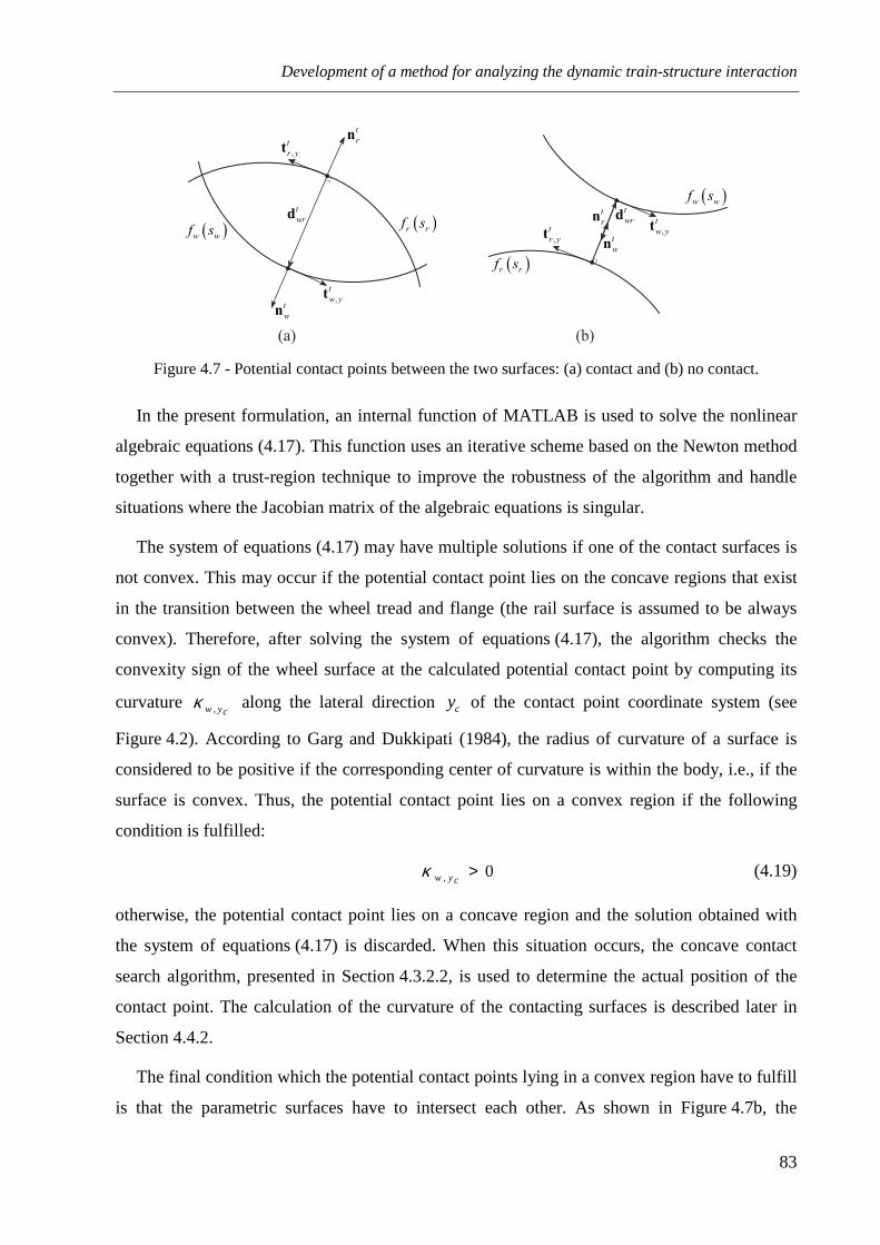
Development of a method for analyzing the dynamic train-structure interaction
83
Figure 4.7 - Potential contact points between the two surfaces: (a) contact and (b) no contact.
In the present formulation, an internal function of MATLAB is used to solve the nonlinear
algebraic equations (4.17). This function uses an iterative scheme based on the Newton method
together with a trust-region technique to improve the robustness of the algorithm and handle
situations where the Jacobian matrix of the algebraic equations is singular.
The system of equations (4.17) may have multiple solutions if one of the contact surfaces is
not convex. This may occur if the potential contact point lies on the concave regions that exist
in the transition between the wheel tread and flange (the rail surface is assumed to be always
convex). Therefore, after solving the system of equations (4.17), the algorithm checks the
convexity sign of the wheel surface at the calculated potential contact point by computing its
curvature cyw,κ along the lateral direction cy of the contact point coordinate system (see
Figure 4.2). According to Garg and Dukkipati (1984), the radius of curvature of a surface is
considered to be positive if the corresponding center of curvature is within the body, i.e., if the
surface is convex. Thus, the potential contact point lies on a convex region if the following
condition is fulfilled:
0, >cywκ (4.19)
otherwise, the potential contact point lies on a concave region and the solution obtained with
the system of equations (4.17) is discarded. When this situation occurs, the concave contact
search algorithm, presented in Section 4.3.2.2, is used to determine the actual position of the
contact point. The calculation of the curvature of the contacting surfaces is described later in
Section 4.4.2.
The final condition which the potential contact points lying in a convex region have to fulfill
is that the parametric surfaces have to intersect each other. As shown in Figure 4.7b, the
(a) (b)
,
t
w yt
,
t
r yt
t
wn
t
rn
t
wrd t
wrdt
rn
,
t
r yt ,
t
w ytt
wn( )w wf s
( )w wf s
( )r rf s
( )r rf s

Chapter 4
84
conditions described in equation (4.17) are satisfied but there is no contact. This condition can
be expressed mathematically as
0≤⋅ tr
twr nd (4.20)
which means that the intersection between two bodies is guaranteed only if the vectors twrd and
trn point in opposite directions, as shown in Figure 4.7a. The penetration d between the two
bodies in contact is given by
twrd d= (4.21)
Since the contact point detection is a nonlinear problem, an initial estimate for the solution
has to be given to start the iterative process. In most cases, in order to reduce the number of
iterations, the solution obtained in the previous iteration/step is used as an initial guess to solve
the current iteration. However, if flange contact occurs, the contact point position suffers an
abrupt jump from the tread to the flange and the previous obtained solution may not be an
appropriate estimation for the current iteration. This can cause the solution to converge very
slowly or even diverge. Therefore, an accurate prediction of jumps in the contact point position
leads to a faster solution and eliminates some of the causes responsible for convergence
problems during the contact solver.
The contact point jump detection proposed in this paper consists of precalculating a lookup
table, similar to those used in the multibody formulations (Santamaria et al., 2006; Tanabe et
al., 2008; Bozzone et al., 2011; Antolín et al., 2012). These lookup tables follow the
assumption of a rigid contact between wheel and rail, in which the surface parameters that
define the contact point position can be computed as a function of the relative lateral
displacement between the center of mass of the wheelset and the track centerline. Thereafter,
the proposed table can predict if there is a contact point in the flange for a given relative lateral
displacement. Since the proposed model is based on the finite element method instead of a
multibody formulation, this table is only used to estimate if there is flange contact. If so, the
surface parameters obtained by table interpolation are used as an initial guess to detect the
potential new flange contact point. This procedure leads to a more accurate initial estimate of
the solution and, consequently, to a higher convergence rate when solving the nonlinear
algebraic equations (4.17). The procedure for implementing the contact lookup table is
described in Appendix A.

Development of a method for analyzing the dynamic train-structure interaction
85
4.3.2.2 Concave contact search
The concave contact approach consists of determining the location of the contact points in
the regions where the convex contact approach cannot find a single solution, i.e., in concave
surfaces (see condition (4.19)). Unlike the algorithm used in the convex contact approach, the
accuracy of this algorithm depends on the degree of discretization of the profiles. Therefore,
although this approach may also be used to locate the contact points in convex regions, the high
computational cost that is required to achieve a good solution makes it computationally less
attractive. As a result, the concave contact approach is used only if the convex approach finds a
solution that lies in a concave region.
In the concave contact search approach, the rail and wheel surfaces are discretized in nr and
nw points, respectively. This discretization is performed by interpolating the profile functions
described in Section 4.3.1, being the position vectors of each point in the rail and wheel
surfaces given by equations (4.9) and (4.15), respectively. Hence, the evaluation of the
potential contact between the two surfaces consists of determining if any of these points lie
inside the opposite surface, forming the so-called intersection volume, illustrated in Figure 4.8.
To determine which points belong to the intersection volume, the points belonging to the rail
surface are projected into the wheel surface and vice-versa. Then, the vertical distances
between the points of each surface and the respective projection on the other surface, irh , and
jwh , , are computed as
( ) rtzt
irt
irir nih ,,2,1,,,, …=⋅−= euu (4.22a)
( ) wtzt
jwt
jwjw njh ,,2,1,,,, …=⋅−= euu (4.22b)
where tir ,u and t
jw,u are the position vectors of the projections along the vertical direction of the
ith rail point into the wheel surface and of the jth wheel point into the rail surface (see
Figure 4.8), respectively, defined with respect to the target element coordinate system, tir ,u and
tjw,u are defined by equations (4.9) and (4.15), respectively, and
tze is a unit base vector of the
target element coordinate system. The point i of the rail surface and the point j of the wheel
surface belong to the intersection volume if the following conditions are fulfilled, respectively:
0, >irh (4.23a)

Chapter 4
86
0, >jwh (4.23b)
Figure 4.8 - Intersection volume: (a) projection of rail points and (b) projection of wheel points.
If there are no points belonging to the intersection volume, the bodies are not in contact and
the potential contact point is discarded from further considerations. On the other hand, when
contact is detected, each point of one of the surfaces belonging to the intersection volume has a
potential contact pair in the other surface. Thus, the potential contact pair of a given point of
the rail surface belonging to the intersection volume is the closest point of the wheel surface,
which also belongs to the intersection volume, and vice-versa. The distance di between the ith
rail point belonging to the intersection volume and the point of the wheel surface j that forms
the potential contact pair is given by
( )[ ] ( )[ ] IVw
IVrtz
tjw
tirty
tjw
tir
ji njnid ,,1and,,1,min
2
,,
2
,, …… ==
⋅−+⋅−= euueuu (4.24)
where IVrn and IV
wn are, respectively, the number of points of the rail and wheel surfaces which
belong to the intersection volume.
Finally, out of all the pairs giving the maximum distance between the rail point and the
correspondent wheel point, the pair where contact occurs is the one that leads to the maximum
penetration d, given by
IVri nidd ,,1,max …== (4.25)
A schematic representation of the selection of the contact pair ij is depicted in Figure 4.9.
i
...
...
... ...
j
...
...
...
...
...
(a) (b)
wf wf
rf rf
,r ih
,w jh
ty
tz
txty
tz
tx
,
t
r iu
,
t
r iu,
t
w ju
,
t
w ju
1i +
1j +
Discretization point
Point projection

Development of a method for analyzing the dynamic train-structure interaction
87
Figure 4.9 - Contact pair selection.
4.4 NORMAL CONTACT PROBLEM
4.4.1 Hertz contact theory
When two non-conforming bodies are compressed against each other they will deform in the
vicinity of the point of first contact, touching over an area that is small when compared with the
dimensions of those bodies and with the relative radii of curvature of the surfaces. On the other
hand, if the shape of the bodies fit exactly at the contact region, a conformal contact occurs,
i.e., the contact between those bodies is not restricted to only one point. In the present method,
the normal contact problem is analyzed based on the nonlinear Hertz theory (Hertz, 1882).
According to the Hertz theory, the contact area between two contacting bodies is elliptical
and the pressure distribution assumes a semi-ellipsoidal shape, being the normal stresses null at
the edges of the contact area and maximum at the center. The assumptions used in the Hertz
theory can be summarized as follows:
a) The surfaces of the bodies are continuous and non-conformal;
b) The surfaces are frictionless;
c) The longitudinal and lateral curvatures of the bodies are constant along the contact area;
d) The contacting bodies are elastic, and no plastic deformations occur in the contact area;
e) The stresses caused by the contact force vanish at a distance far from the contact area;
f) The contacting bodies can be considered as elastic half-spaces.
Note that, in a wheel-rail contact problem, the assumptions of the Hertz theory are not met,
since the surfaces of the contacting bodies are not totally frictionless and may be conforming.
i
j
i=1i=2
j=1 j=2
......
...
...
...
...
...
...
...
......
...
d
IV
rn
IV
wn
wfrf
Contact point
Potential contact point

Chapter 4
88
Moreover, the wheel and rail profiles may have non-constant curvatures in the contact area and
plastic deformations may occur in the contact zone. Nevertheless, in most railway applications,
the Hertz theory seems to be sufficiently adequate for the computation of the normal contact
forces during a dynamic analysis (Andersson et al., 1999). More complex and realistic contact
shapes may be necessary for analyzing local problems, such as wear. However, this is out of
the scope of the present thesis.
4.4.2 Geometry of the surfaces in contact
Following the aforementioned assumptions, Hertz assumed that the surfaces of the
contacting bodies (see Figure 4.10) may be expressed as
211
2111 yBxAz += (4.26a)
222
2222 yBxAz += (4.26b)
where ix and iy are the directions of the principal curvatures of body i and iA and iB are
constants that depend on the body i geometry (i = 1, 2). The gap between the two bodies is
defined as
21 zzh −= (4.27)
which can be rewritten as
yxCyBxAh ++= 22 (4.28)
where x and y are the directions which form an angle α and β with the principal directions of
the bodies 1 and 2, respectively (see Figure 4.10).
Figure 4.10 - Two bodies in contact and their respective principal directions and radii of curvature.
x
y
z
αβ2x
1y
2y
1x
h
1, yR
1,xR
2,xR 2, yR
Body 1
Body 2

Development of a method for analyzing the dynamic train-structure interaction
89
Considering the principal radii of curvature of the surfaces (see Figure 4.10), equations (4.26)
and (4.28) are rewritten in the form
21
,1
21
,11 2
1
2
1y
Rx
Rz
yx
+= (4.29a)
22
,2
22
,22 2
1
2
1y
Rx
Rz
yx
+= (4.29b)
yxCyR
xR
hyx
++= 22
2
1
2
1 (4.30)
where xiR , and yiR , are the principal radii of curvature of the body i (i = 1, 2) and xR and yR
are the principal relative radius of curvature.
The angles α and β may be calculated by eliminating the quadratic term xy from equation
(4.30). Using this, in addition to the equation (4.29), the following relations are obtained
(Hertz, 1882; Johnson, 1985; Shabana et al., 2008)
( ) ( )βα 2cos11
2
12cos
11
2
1
,2,2,1,1
−+
−=−
yxyx RRRRAB (4.31a)
+++=+
yyxx RRRRBA
,2,1,2,1
1111
2
1 (4.31b)
When the relative yaw rotations between wheel and rail are small, which occurs in the
majority of the wheel-rail contact problems, the α and β angles may be neglected (Antolín,
2013). With this assumption, the geometric parameters A and B are given by
+=
xx RRA
,2,1
11
2
1 (4.32a)
+=
yy RRB
,2,1
11
2
1 (4.32b)
Note that in this case, the principal directions x and y coincide with the principal directions of
both contacting bodies.
The radius of curvature is defined as the inverse of the curvature in the respective direction.
Thus, taking the body 1 and 2 as the wheel and rail, respectively, and the principal directions x
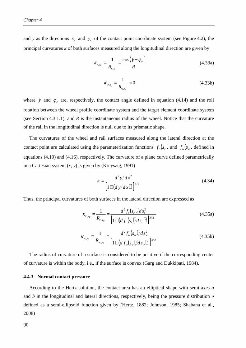
Chapter 4
90
and y as the directions cx and cy of the contact point coordinate system (see Figure 4.2), the
principal curvatures κ of both surfaces measured along the longitudinal direction are given by
( )RR
w
cxrcxr
φγκ −== cos1
,, (4.33a)
01
,, ≈=
cxwcxw R
κ (4.33b)
where γ and wφ are, respectively, the contact angle defined in equation (4.14) and the roll
rotation between the wheel profile coordinate system and the target element coordinate system
(see Section 4.3.1.1), and R is the instantaneous radius of the wheel. Notice that the curvature
of the rail in the longitudinal direction is null due to its prismatic shape.
The curvatures of the wheel and rail surfaces measured along the lateral direction at the
contact point are calculated using the parameterization functions ( )rr sf and ( )ww sf defined in
equations (4.10) and (4.16), respectively. The curvature of a plane curve defined parametrically
in a Cartesian system (x, y) is given by (Kreyszig, 1991)
( )[ ] 232
22
1 xdyd
xdyd
+=κ (4.34)
Thus, the principal curvatures of both surfaces in the lateral direction are expressed as
( )
( )( )[ ] 232
22
,,
1
1
rrr
rrr
cyrcyr
sdsfd
sdsfd
R +==κ (4.35a)
( )
( )( )[ ] 232
22
,,
1
1
www
www
cywcyw
sdsfd
sdsfd
R +==κ (4.35b)
The radius of curvature of a surface is considered to be positive if the corresponding center
of curvature is within the body, i.e., if the surface is convex (Garg and Dukkipati, 1984).
4.4.3 Normal contact pressure
According to the Hertz solution, the contact area has an elliptical shape with semi-axes a
and b in the longitudinal and lateral directions, respectively, being the pressure distribution σ
defined as a semi-ellipsoid function given by (Hertz, 1882; Johnson, 1985; Shabana et al.,
2008)
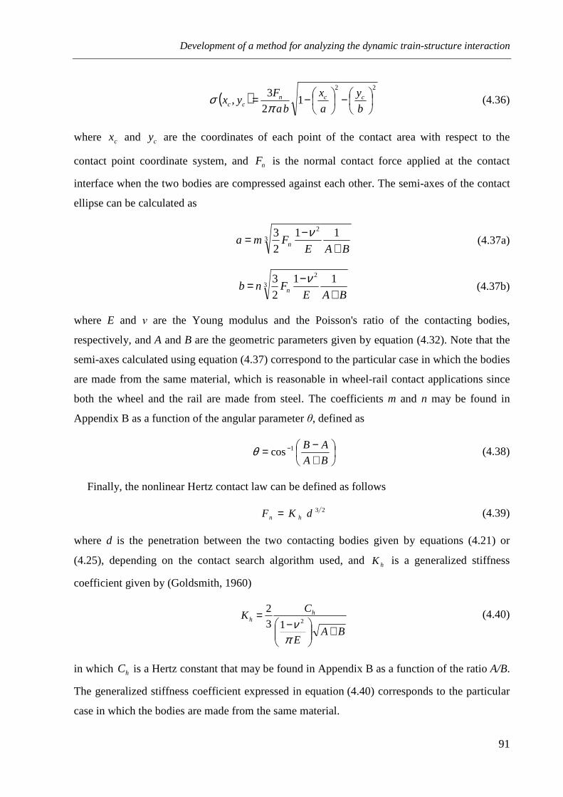
Development of a method for analyzing the dynamic train-structure interaction
91
( )22
12
3,
−
−=b
y
a
x
ba
Fyx ccn
cc πσ (4.36)
where cx and cy are the coordinates of each point of the contact area with respect to the
contact point coordinate system, and nF is the normal contact force applied at the contact
interface when the two bodies are compressed against each other. The semi-axes of the contact
ellipse can be calculated as
3
2 11
2
3
BAEFma n +
−= ν (4.37a)
3
2 11
2
3
BAEFnb n +
−= ν (4.37b)
where E and ν are the Young modulus and the Poisson's ratio of the contacting bodies,
respectively, and A and B are the geometric parameters given by equation (4.32). Note that the
semi-axes calculated using equation (4.37) correspond to the particular case in which the bodies
are made from the same material, which is reasonable in wheel-rail contact applications since
both the wheel and the rail are made from steel. The coefficients m and n may be found in
Appendix B as a function of the angular parameter θ, defined as
+−= −
BA
AB1cosθ (4.38)
Finally, the nonlinear Hertz contact law can be defined as follows
23dKF hn = (4.39)
where d is the penetration between the two contacting bodies given by equations (4.21) or
(4.25), depending on the contact search algorithm used, and hK is a generalized stiffness
coefficient given by (Goldsmith, 1960)
BAE
CK h
h
+
−=
πν 213
2 (4.40)
in which hC is a Hertz constant that may be found in Appendix B as a function of the ratio A/B.
The generalized stiffness coefficient expressed in equation (4.40) corresponds to the particular
case in which the bodies are made from the same material.

Chapter 4
92
4.5 TANGENTIAL CONTACT PROBLEM
4.5.1 Creep phenomenon
If two bodies that are compressed against each other are allowed to roll over each other,
some points on the contact area may slip while others may adhere (see Figure 4.11). The
difference between the tangential strains of the bodies in the adhesion area leads to a small
apparent slip, called creep. The creep, which depends on the relative velocities of the two
bodies at the contact point, is crucial for the determination of the tangential forces that develop
in the contact area, called creep forces. Hence, the creep may be defined as a combined elastic
and frictional behavior in which two elastic bodies that roll over each other share a contact area
where both slip and adhesion occur simultaneously. This phenomenon was recognized for the
first time by Carter (1926).
A typical distribution of normal and tangential stresses inside an elliptical contact area Γ
defined by the Hertz theory is illustrated in Figure 4.11.
Figure 4.11 - Distribution of normal and tangential stresses inside the contact area.
Let ABC be a line inside the contact ellipse along the longitudinal direction. The tangential
stresses τ, which are null in the leading edge (point A), tend to grow as approaching the limit of
the Coulomb law limτ in point B, given by
σµτ =lim (4.41)
B AC
Adhesionregion
Slipregion
Leading edge
a
b
Coulomb's tangential
stress limit
cx
cy
cx
,σ τ
τ µ σ=τ µ σ<
σ
Rear edgeΓ

Development of a method for analyzing the dynamic train-structure interaction
93
where µ is the friction coefficient and σ the normal stresses given by equation (4.36). In this
region of the contact area, called adhesion region, the wheel and rail stick to each other, being
their relative displacements fully compensated by the elastic strain of the bodies. However,
from point B to point C, the normal stresses are no longer capable of supporting the strains and
the wheel and rail start to slide, forming the slip region of the contact area in which relative
motions between the two bodies occur.
4.5.2 Basic equations of the rolling contact
The relative velocity between wheel and rail at the contact area may be determined as a
function of three dimensionless parameters, called creepages, defined with respect to the
contact point coordinate system presented in Figure 4.2. These are the longitudinal creepage ,ξυ
the lateral creepage ηυ and the angular slip velocity around an axis perpendicular to the contact
area, called spin creepage φυ , as depicted in Figure 4.12. The creepages are necessary for the
calculation of the tangential forces that develop in the contact area, called creep forces.
Figure 4.12 - Orientation of the creepages with respect to the contact point coordinate system.
The longitudinal and the lateral creepages are the relative velocities between the wheel and
rail at the contact point along the cx and cy axes, respectively, normalized to the vehicle's
speed V, given by
( )
Vcxrw eaa ⋅−
=ɺɺ
ξυ (4.42a)
( )
Vcyrw eaa ⋅−
=ɺɺ
ηυ (4.42b)
cz
cx
cy
Contact area Γ
φυ
ξυ
ηυ

Chapter 4
94
where waɺ and raɺ are the vectors of translational velocities of the wheel and rail at the contact
point, respectively, defined with respect to the global coordinate system, and cxe and
cye are
unit base vectors of the contact point coordinate system.
The spin creepage is the relative angular velocity between the wheel and rail at the contact
point about the cz axis normalized to the vehicle's speed, given by
( )
Vczrw eωω ⋅−
=ɺɺ
φυ (4.43)
in which wωɺ and rωɺ are the vectors of rotational velocities of the wheel and rail at the contact
point, respectively, defined with respect to the global coordinate system, and cze is a unit base
vector of the contact point coordinate system.
Using the creepages defined in equations (4.42) and (4.43), the rigid body slip rɺ at each
point of the contact area is found to be (Garg and Dukkipati, 1984; Kalker, 1990)
( ) ( )( )
+−
=
=
c
c
cy
cx
cc xV
yV
r
ryx
φη
φξ
υυυυ
ɺ
ɺ
ɺ ,r (4.44)
where cx and cy are the coordinates of an arbitrary point of the contact area with respect to the
contact point coordinate system. Furthermore, as a consequence of compressive and frictional
forces in the contact area, local elastic deformations occur in the wheel and rail surfaces. Thus,
the relative tangential elastic displacements v at each point of the contact area may be
expressed as (Kalker, 1990)
( ) ( ) ( )ccrccw
cy
cx
cc yxyxv
vyx ,,, vvv −=
= (4.45)
where wv and rv are, respectively, the elastic surface displacements of the wheel and rail at
the contact area. Hence, the actual slip sɺ , which represents the relative velocity between a
particle of the wheel inside the contact area and the corresponding contact particle of the rail, is
given by (Garg and Dukkipati, 1984; Kalker, 1990)
vrs ɺɺɺ += (4.46)
where vɺ is the derivative of v with respect to time. Considering that the contact area moves
with the wheel in the longitudinal direction cx , equation (4.46) may be rewritten as

Development of a method for analyzing the dynamic train-structure interaction
95
t
Vxc ∂
∂+∂∂−= vv
rs ɺɺ (4.47)
which in the case of steady-state rolling, the component t∂∂v is null. In the wheel-rail contact
area, the actual slip sɺ , the tangential stress τ and the normal pressure σ are related by the
Coulomb law as (Kalker, 1990)
≠=
=≤
region) (slip0if
region)(adhesion 0if
sτ
sτ
ɺ
ɺ
σµµ
(4.48)
Finally, the longitudinal ξF and lateral ηF creep forces, as well as the spin creep moment
φM , can be calculated by integrating the tangential stresses along the contact area Γ as follows
(Kalker, 1990):
∫∫Γ
= cccx dydxF τξ (4.49a)
∫∫Γ
= cccy dydxF τη (4.49b)
( )∫∫Γ
−= cccxccyc dydxyxM ττφ (4.49c)
where cxτ and
cyτ are the longitudinal and lateral components of the tangential stress vector τ.
4.5.3 Creep force theories
In Section 2.4.3 of Chapter 2, several wheel-rail rolling contact theories, used to calculate
the creep forces that develop at the contact interface, are introduced and briefly described.
Among these, the Kalker's linear theory (Kalker, 1967), the Polach method (Polach, 1999) and
the Kalker's book of tables (Kalker, 1996) are implemented in the vehicle-structure interaction
method proposed in the present chapter.
4.5.3.1 Kalker's linear theory
According to Kalker's linear theory (Kalker, 1967), the actual slip sɺ inside the contact area
is null (no-slip condition) and the adhesion region is assumed to cover the entire contact area.
Thus, by imposing this condition to equation (4.47), one obtains
cc
cx yx
vφξ υυ −=
∂∂
(4.50a)

Chapter 4
96
cc
cy xx
vφη υυ +=
∂∂
(4.50b)
Integrating equation (4.50) with respect to cx gives
( )cccccx yfxyxv 1+−= φξ υυ (4.51a)
( )ccccy yfxxv 22
2
1 +−= φη υυ (4.51b)
where ( )cyf1 and ( )cyf2 are arbitrary functions that arise from the integration process.
For an elliptical contact area, and according to the Galin theorem (Kalker, 1967), if the
distribution of the relative tangential elastic displacements v is described by a polynomial
function, the tangential stresses can be as well, but multiplied by
( )22
1
1,
−
−
=
b
y
a
xyxJ
cc
cc (4.52)
As a consequence of the no-slip condition, the tangential stresses must be continuous at the
leading edge of the contact area, which implies that it vanishes at that point. Hence, according
to the aforementioned distribution of the tangential stresses, the creep forces law expressed in
equation (4.49) may be defined as
ξξ υ11cbaGF −= (4.53a)
( )φηη υυ 2322 cbacbaGF +−= (4.53b)
( )φηφ υυ 3323 cbacbabaGM +−−= (4.53c)
where G is the combined shear modulus of rigidity of wheel and rail materials and cij are
Kalker's creepage coefficients that depend on the semi-axes ratio a/b and on the Poisson's ratio
of the wheel and rail materials. These coefficients can be found in Appendix B
Note that the linear theory is an approximation, since for large creepages the condition given
by the Coulomb's law can be violated. Nevertheless, due to its low computational cost, the
linear theory may be useful to study scenarios in which the creepages remain low, such as
railway operations in ordinary conditions.

Development of a method for analyzing the dynamic train-structure interaction
97
4.5.3.2 Polach method
Polach (1999) proposed an algorithm to compute the wheel-rail creep forces based on the
Hertz assumption of an elliptical contact area, in which the relative displacements between the
bodies in the adhesion region increase linearly from the leading to the rear edge. Thus, the
tangential stress also grows linearly with the distance from the leading edge, being its
maximum limited by the Coulomb's law, as stated in equation (4.41). If the tangential stress in
the adhesion region reaches the maximum value, sliding takes place and a slip region begins to
form, as depicted in Figure 4.11.
According to Polach (1999), the tangential contact force trF due to the translational
creepages ξυ and ηυ is given by
+
+−= −
trtr
trntr
FF ε
εε
πµ 1
2tan
1
2 (4.54)
in which trε is the gradient of tangential stress in the adhesion region given by
trCn
Ctr F
cbaG υµ
πε4
1= (4.55)
where Cc is a constant that depends on the Kalker's creepage coefficients 11c and 22c as
follows
2
22
2
11
+
=
trtrC ccc
υυ
υυ ηξ (4.56)
and trCυ is the modified translational creepage, which accounts for the effect of the spin
creepage, that can be written as
22CtrC ηξ υυυ += (4.57)
In equation (4.56), the parameter trυ is the magnitude of the translational creepage given by
22ηξ υυυ +=tr (4.58)
while Cηυ , presented in equation (4.57), is the modified lateral creepage defined as
>++
≤+=
ηφηφη
ηφηηη
υυυυυ
υυυυυ
aa
aC
if
if (4.59)

Chapter 4
98
Assuming that the creep moments are small when compared to other moments acting on the
system, the lateral tangential contact force SFη caused by pure spin is found to be
( )[ ]baMnS eKFaF −−+−= 13.61
16
9 µη (4.60)
where MK is defined as
( )3223
13
1
6
1
23δδδε −−
+−= SMK (4.61)
and δ is given by
1
12
2
+−=
S
S
εεδ (4.62)
The parameter Sε is the gradient of tangential stress to account for the spin influence that is
given by
( )ba
C
nS
e
c
F
babG−−+
=13.613
8 23 ηυµ
ε (4.63)
in which 23c is one of the Kalker's creepage coefficient.
Finally, the creep forces according to the Polach's method are defined as
trC
trFFυυξ
ξ = (4.64a)
( )φηηη υυυ Str
trC
FFF += 1 (4.64b)
Note that the contribution of spin is accounted for in the lateral creep force. According to
Polach (1999), the moment caused by the spin and lateral creepages can be neglected, since it is
small when compared to other moments acting on the system.
4.5.3.3 Kalker's book of tables
Kalker (1996) proposed a methodology based on precalculated lookup tables, named book
of tables, in which several values of creep forces are stored to be later interpolated during the
dynamic analysis as a function of the creepages and the semi-axes ratio of the contact ellipse.
Development of a method for analyzing the dynamic train-structure interaction
99
The tables, along with the algorithm to interpolate them, were implemented in a computer code
called USETAB.
The lookup table uses an effective layout, exploiting all possible symmetries between the
contact forces and creepages (Kalker, 1967). The values from the table are normalized and
calculated according to the following criteria: 1) the combined shear modulus of the wheel and
rail materials G is 1; 2) the Coulomb's friction limit given by nFµ is 1 and 3) the square root of
the ellipse's semi-axes product ab is 1. The table inputs are the semi-axes ratio of the contact
ellipse and the normalized creepages, defined as
ξξ υµ
υ 113c
F
Gba
n
=′ (4.65a)
ηη υµ
υ 223c
F
Gba
n
=′ (4.65b)
( )
φφ υµ
υ 23
23
cF
Gba
n
=′ (4.65c)
The outputs consist in the normalized longitudinal creep force ξF ′ , the normalized lateral creep
force ηF ′ and the normalized spin creep moment φM ′ , which are linearly interpolated during the
dynamic analysis. Hence, the absolute value of the creep forces are given by
nFFF µξξ ′= (4.66a)
nFFF µηη ′= (4.66b)
abFMM nµφφ ′= (4.66c)
In the present thesis, the table is calculated using the software CONTACT (2011) which is
based on Kalker's exact three-dimensional rolling contact theory (Kalker, 1979). The
normalized creepages and semi-axes ratios were discretized in two intervals as in the original
USETAB, namely 10 ≤≤ x and ∞<≤ x1 , where x is the input of the table. However, a linear
and a logarithmic distribution of ten values were used for the discretization of the first and
second intervals, respectively, instead of the original linear intervals with seven values.
Adopting a 4040× element discretization of the contact ellipse, and by considering all possible
combinations of the creepages and semi-axes ratios, a total of 000320 calculations were
performed using the software CONTACT.

Chapter 4
100
An important point is the consideration of an upper limit for the table to avoid inaccurate
extrapolations. Furthermore, according to Kalker (1996), the linear interpolations with
semi-axes ratios close to zero or infinite should be avoided, since the creepage coefficients are
singular in these cases. Therefore, an upper limit of 103 and a lower limit of 10-3 are used for
the semi-axes ratios and an upper limit of 103 is adopted for the normalized creepages. If a
combination of creepages and semi-axes ratio falls outside these intervals, the Polach method is
used to solve the mentioned singularities.
4.6 FORMULATION OF THE TRAIN-STRUCTURE COUPLING SYSTEM
Neves et al. (2012) developed an algorithm, referred to as the direct method, in which the
governing equilibrium equations of the vehicle and structure are complemented with additional
constraint equations that relate the displacements of the contact nodes of the vehicle with the
corresponding nodal displacements of the structure, with no separation being allowed. These
equations form a single system, with displacements and contact forces as unknowns, that is
solved directly using an optimized block factorization algorithm. Later, Neves et al. (2014)
extended the algorithm to deal with wheel-rail separation. In this approach, a search algorithm
is used to detect which wheels are in contact, being the constraint equations only imposed when
contact occurs. Finally, Montenegro et al. (2015b) included the lateral dynamic effects between
railway vehicles and structures by incorporating the wheel-rail contact model described above.
4.6.1 Governing equations of motion
4.6.1.1 Force equilibrium
Considering the α method (Hughes, 2000), the equations of motion of the vehicle-structure
system can be written as
( ) ( ) tttttttt αααα FFRRaM −+=−++ ∆+∆+∆+ 11ɺɺ (4.67)
where M is the mass matrix, R are the nodal forces corresponding to the internal element
stresses, F are the externally applied nodal loads and a are the nodal displacements. The elastic
and damping forces depend nonlinearly on the nodal displacements and velocities due to the
several nonlinearities considered in the present formulation, such as the wheel-rail contact and
the nonlinear suspensions. In the present work, the nonlinear inertia effects, such as the

Development of a method for analyzing the dynamic train-structure interaction
101
centrifugal and gyroscopic effects, are neglected. The superscripts t and tt ∆+ indicate the
previous and current time step, respectively.
To solve equation (4.67) let the F type degrees of freedom (DOF) represent the free nodal
DOF, whose values are unknown, and the P type DOF represent the prescribed nodal DOF,
whose values are known. Thus, the load vector can be expressed as
teteFX
ceceFXFF XDXDPF ++= (4.68a)
SXDPF ++= tetePXPP (4.68b)
where P corresponds to the externally applied nodal loads whose values are known, S are the
support reactions and X are the forces acting at the contact interface shown in Figure 4.1. Each
matrix D relates the contact forces, defined with respect to the target element coordinate
system, with the nodal forces defined in the global coordinate system.
According to Newton’s third law, the forces acting at the contact interface must be of equal
magnitude and opposite direction (see Figure 4.1), i.e.,
0XX =+ tece (4.69)
Substituting equation (4.69) into equation (4.68) leads to
XDPF FXFF += (4.70a)
SXDPF ++= PXPP (4.70b)
where
ceXX = (4.71)
teFX
ceFXFX DDD −= (4.72)
tePXPX DD −= (4.73)
Substituting equation (4.70) into equation (4.67), and partitioning into F and P type DOF,
gives
( )
( )
+++
−
+++
+=
−
++
∆+∆+∆+∆+
∆+∆+∆+
∆+
∆+
∆+
∆+
tttPX
tP
ttFX
tF
ttttttPX
ttP
ttttFX
ttF
tP
tF
ttP
ttF
ttP
ttF
PPPF
FPFF
αα
αα
SXDP
XDP
SXDP
XDP
R
R
R
R
a
aMM
MM
1
1ɺɺ
ɺɺ
(4.74)
Chapter 4
102
Considering only the first row of equation (4.74) and transferring the unknowns to the
left-hand size leads to
( ) ( ) Ftttt
FXtt
Ftt
FFF αα FXDRaM =+−++ ∆+∆+∆+∆+ 11ɺɺ (4.75)
where
( ) tF
ttPFP
ttFX
tF
ttFF αααα RaMXDPPF +−−−+= ∆+∆+
ɺɺ1 (4.76)
4.6.1.2 Incremental formulation for nonlinear analysis
Since the present problem has a nonlinear nature, equation (4.75) is rewritten in the form
( ) 0Xaψ =∆+∆+ ttttFF , (4.77)
where Fψ is the residual force vector, given by
( ) ( ) ( ) ttttFX
ttF
ttFFFF
ttttFF αα ∆+∆+∆+∆+∆+∆+ +++−−= XDRaMFXaψ 11, ɺɺ (4.78)
The nodal velocities and accelerations depend on the nodal displacements and for this reason
are not independent unknowns. According to the α method, the following approximations for
the acceleration and velocity at the current time step can be obtained (Neves et al., 2014):
( ) ttttttt aβ
atβ
aatβ
a ɺɺɺɺɺ
−−
∆−−
∆= ∆+∆+ 1
2
1112 (4.79)
( ) ttttttt aβ
γta
β
γaa
tβ
γa ɺɺɺɺ
−∆+
−+−
∆= ∆+∆+
211 (4.80)
where β and γ are parameters that control the stability and accuracy of the method.
An iterative scheme based on the Newton method (Owen and Hinton, 1980) is used to solve
equation (4.77). Assuming that the solution at the ith Newton iteration has been evaluated and
neglecting second and higher order terms, the Taylor series for Fψ about ( )ittittF
,, , ∆+∆+ Xa is
given by
( ) ( ) ( )
( )ittitt
ittittF
ttF
ittF
ittF
ittittF
ttF
FittittFF
ittittFF
,1,
,,,
,1,
,,,
,,1,1, ,,
∆++∆+
∆+∆+
∆+
∆++∆+
∆+∆+
∆+∆+∆++∆++∆+
−
∂∂+
−
∂∂+=
XXXψ
aaaψ
XaψXaψ
Xa
Xa
(4.81)

Development of a method for analyzing the dynamic train-structure interaction
103
Substituting equations (4.78) to (4.80) into equation (4.81), and assuming that the residual
force vector at iteration i+1 fulfils the condition given by equation (4.77), leads to
( ) ( ) ( )
( ) ( ) 0XXD
aaaR
MXaψ
a
=−++
−
∂∂+−
∆−+
∆++∆+∆+
∆++∆+
∆+∆+
∆+∆+
ittittittFX
ittF
ittF
ittF
ttF
FFF
ittittFF
α
αtβ
,1,,
,1,
,2
,,
1
11
, (4.82)
Transforming equation (4.82) into an incremental form leads to
( ) iF
iittFX
iFFF α ψXDaK =∆+−∆ +∆++ 1,1 1 (4.83)
where FFK is the current effective stiffness matrix defined by
( )
∂∂++
∆=
∆+∆+
ittF
ttF
FFFFF α
tβ ,2 1
1
aaR
MK (4.84)
and
ittF
ittF
iF
,1,1 ∆++∆++ −=∆ aaa (4.85)
ittitti ,1,1 ∆++∆++ −=∆ XXX (4.86)
( )ittittFF
iF
,, , ∆+∆+= Xaψψ (4.87)
In matrix notation, equation (4.83) can be expressed as
[ ] iFi
iF
FXFF ψX
aDK =
∆∆
+
+
1
1
(4.88)
being
( ) ittFXFX
,1 ∆++−= DD α (4.89)
After evaluating the solution at iteration i+1, the residual force vector is calculated using
equation (4.78). The iteration scheme continues until the following condition is fulfilled:
ε≤∆+
+
ttF
iF
P
ψ1
(4.90)
where ε is a specified tolerance.

Chapter 4
104
4.6.1.3 Updating of the effective stiffness matrix
According to Owen and Hinton (1980), the complete factorization of the global effective
stiffness matrix (full Newton-Raphson method) can be avoided if the stiffness corresponding to
the initial trial of the iterative process is kept constant. This procedure, called initial stiffness
method, has the immediate advantage of significantly reducing the computational cost of each
iteration but reduces the convergence rate of the step, since more iterations are required to
achieve the necessary convergence expressed in equation (4.90). Thus, the optimal algorithm is
generally provided by a combination of these two processes, depending on the degree of
nonlinearity inherent in the problem.
In the present work, the main nonlinearities inherent to the problem are concentrated at the
wheel-rail contact elements described in Section 4.2. Regarding the stiffness of these elements,
since the Hertz law (Hertz, 1882) is given by the close-form expression presented in
equation (4.39), which has an analytic derivative, the tangent stiffness matrix K can be updated
at each iteration in order to take advantage of the full Newton-Raphson method. However, the
same is not true regarding the damping, since the contact laws based on Kalker's exact theory
of rolling contact (Kalker, 1979) or on Polach's method (Polach, 1999) cannot be defined with a
closed-form expression. Therefore, since the calculation of numerical derivatives with respect
to the nodal velocities can be computationally expensive, the initial tangent damping matrix C
of the contact element is calculated based on the Kalker's linear theory (Kalker, 1967) and is
kept constant throughout the analysis.
4.6.2 Contact constraint equations
When contact occurs, the additional internal node of the contact element and the auxiliary
point belonging to the rigid surface of the target element are coupled in the three directions (see
Section 4.2). Thus, the following constraint equations must be imposed:
rvv =− tece (4.91)
where r are the irregularities between the contact and target elements in the vertical and lateral
directions. The displacements of the additional internal nodes (see Figure 4.1) are given by
1, +∆+= ittF
ceXF
ce aHv (4.92)
where the transformation matrix H relates the displacements of the additional internal nodes of
the contact element, defined in the global coordinate system, with the displacements defined in
Development of a method for analyzing the dynamic train-structure interaction
105
the local coordinate system of the corresponding target element. The displacements of the
auxiliary points of the target elements are given by
ttP
teXP
ittF
teXF
te ∆++∆+ += aHaHv 1, (4.93)
where each transformation matrix H relates the displacements of the nodes of the target
elements, defined in the global coordinate system, to the displacements of the auxiliary points
defined in the target element coordinate system.
Substituting equations (4.92) and (4.93) into equation (4.91) yields
ttPXP
ittFXF
∆++∆+ −= aHraH 1, (4.94)
where
teXF
ceXFXF HHH −= (4.95)
teXPXP HH −= (4.96)
Rearranging equation (4.85) in terms of 1, +∆+ ittFa and substituting into equation (4.94) leads to
ittFXF
ttPXP
iFXF
,1 ∆+∆++ −−=∆ aHaHraH (4.97)
Multiplying equation (4.97) by ( )α+− 1 gives
raH =∆ +1iFXF (4.98)
where
( ) XFXF α HH +−= 1 (4.99)
and
( ) ( )ittFXF
ttPXPα ,1 ∆+∆+ −−+−= aHaHrr (4.100)
4.6.3 Complete system of equations
The incremental formulation of the governing equations of motion of the vehicle-structure
system is applicable to either linear or nonlinear analyses. These equations and the contact
constraints form a complete system whose unknowns are incremental nodal displacements and
incremental contact forces. Equations (4.88) and (4.98) can be expressed in matrix form leading
to the following system of equations:
=
∆∆
+
+
r
ψ
X
a
0H
DK iF
i
iF
XF
FXFF
1
1
(4.101)

Chapter 4
106
Using Betti’s theorem, it can be demonstrated that the matrix in equation (4.101) is
symmetric. Since the time required to solve the system of linear equations presented in
equation (4.101) may represent a significant percentage of the total solution time, the efficiency
of the solver is very important. The system matrix is partitioned into the following form in
order to improve the efficiency of the solver.
=
∆∆∆∆
+
+
+
+
r
ψ
ψ
ψ
X
a
a
a
0HHH
DKKK
DKKK
DKKK
iY
iR
iI
i
iY
iR
iI
XYXRXI
YXYYYRYI
RXRYRRRI
IXIYIRII
1
1
1
1
(4.102)
The F type DOF is partitioned into I, R and Y type DOF. The Y type DOF corresponds to the
DOF of the internal nodes added by the contact elements (see node C3 in Figure 4.1). These
DOF have to be grouped together because they are only active when contact occurs, and so the
size of the matrices relating these DOF is time-dependent. Since the laws for the contact
interface are nonlinear, the matrices of the contact elements are also time-dependent. The R
type DOF correspond to all the nodal DOF of the contact elements, except for the Y type DOF,
which have already been grouped separately (see node C1 in Figure 4.1). The I type DOF are all
the remaining F type DOF. The R type DOF can also include DOF belonging to other nonlinear
finite elements such as the spring-dampers used to model the vehicle's suspensions. The present
method adopts a block factorization algorithm (see Appendix C), based on that developed
by Neves et al. (2012) and later extended by Montenegro et al. (2015b) to deal with 3D contact.
4.6.4 Algorithm for solving the train-structure interacti on problem
The proposed train-structure interaction method is implemented in MATLAB, being the
vehicles and structures modeled with ANSYS. All the data regarding these models, such as the
structural matrices, the definition of the target elements, the contact nodes of the vehicle and
the support conditions are exported using ANSYS in batch mode and subsequently imported by
MATLAB. The remaining data, namely the irregularities between the wheel and rail, the
contact lookup table and the control points defining the rail and wheel profiles are stored in an
external database and imported directly by MATLAB.
After all the data is imported and processed, an initial static analysis is performed in order to
obtain the initial conditions of the dynamic problem. The flowchart depicted in Figure 4.13
illustrates all the aspects regarding the dynamic analysis of the train-structure interaction.

Development of a method for analyzing the dynamic train-structure interaction
107
Figure 4.13 - Flowchart of the algorithm for analyzing the train-structure dynamic interaction.
Calculate
Start
Predict: a) ; b)
Contact occurs
Update matrices D and H
Calculate the internal resisting forces in the normal direction
Calculate creepages (Eq. 4.42 and 4.43)
and ellipse’s semi-axes (Eq. 4.37)
Calculate the internal resisting forces in the tangential directions
Estimate
End
No contact occurs
Update matrices D and H
Solve system of equations (4.102) (see Appendix B)
Update:
a)
b) (Eq. 4.80)
c) (Eq. 4.79)
d)
YesNo
Yes
No
No
True
Yes
False
( )0
,r w treads s
0t =
t t+∆P
t tF+∆ =a 0ɺɺ
t t t+∆ =X X
( ) 21 2t t t t tF F F Ft tβ+∆ = + ∆ + − ∆a a a aɺ ɺɺ
( )1t t t tF F F tγ+∆ = + − ∆a a aɺ ɺ ɺɺ
0i =
Wheel 1i =
Wheel Wheeli n=
endt t=
Update (Eq. 4.84) FFK
, 1t t iF+∆ +
aɺɺ
, 1 , 1t t i t t i i+∆ + +∆ += + ∆X X X
, 1t t iF+∆ +
aɺ
, 1 , 1t t i t t i iF F F+∆ + +∆ += + ∆a a a
1i i= +
Wheel Wheel 1i i= +
Wheel Wheel 1i i= +t t t= + ∆
(Eq. 4.19)
Convex contact
search (Section 4.3.2.1)
Concave contact
search (Section 4.3.2.2)
No Yes, 0w yc
κ >
Contact status (Eq. 4.20 or 4.23)
( ) ( )1
, ,i i
r w r wtread treads s s s
+=
( ) ( )1
, ,i i
r w r wflange flanges s s s
+= or contact tables
t tF ε+∆ ≤Pψ
Fi+1
(Eq. 4.90)
Calculate (Eq. 4.78) ( )tttt
FF
∆+∆+Xaψ ,

Chapter 4
108
4.7 CONCLUDING REMARKS
A method for analyzing the nonlinear dynamic interaction between the train and structure is
proposed and implemented (Montenegro et al., 2015b). The method takes into account the
geometry of the wheel and rail surfaces in order to accurately evaluate the lateral interaction.
In the majority of the currently available methods for analyzing the train-structure
interaction, the normal and tangential contact forces are treated as external forces. However, it
is generally more efficient to use a finite element formulation based on the contact laws for the
normal and tangential directions. Therefore, a wheel-rail contact finite element specially
developed for modeling the behavior of the contact interface in the normal and tangential
directions is proposed. This behavior is reproduced by a wheel-rail contact model whose
formulation is divided in three main parts: the geometric problem, the normal problem and the
tangential problem.
The geometric problem, which consists of detecting the position of the contact points
between wheel and rail, is solved online, i.e., during the dynamic analysis. Although this
procedure is computationally more expensive than an offline contact approach, in which the
location of the contact points is precalculated as a function of the relative displacements
between wheel and rail, its higher accuracy outweighs this drawback. The proposed method is
able to look for potential contact points in any type of geometric surfaces (convex or concave)
at the tread and the flange of the wheel. Thus, the formulation is suitable to investigate not only
scenarios related to ordinary railway operation, but also derailment situations, in which the
flange contact plays an important role.
Regarding the normal contact problem, the nonlinear Hertz theory is used to compute the
normal contact forces between wheel and rail. Although this theory rests on a series of
assumptions that may limit its range of application, it offers a good compromise between
computational efficiency and accuracy for dealing with the dynamic analysis of railway
vehicles. However, for the study of local phenomena, such as wear, a more accurate procedure
based on multi-Hertzian or non-Hertzian formulations may be adopted.
For dealing with the tangential contact problem, three different approaches are adopted.
Since the exact theory of rolling contact proposed by Kalker (1979) is impracticable to be used
in dynamic analysis of railway vehicles due to its excessive computational cost, the Polach
method (Polach, 1999), the Kalker's book of tables (Kalker, 1996) and the Kalker's linear

Development of a method for analyzing the dynamic train-structure interaction
109
theory (Kalker, 1967) are implemented in the proposed formulation. The first two methods
combine accuracy with computational efficiency, while the latter is limited to scenarios with
small creepages. However, due to its excellent computational performance, the Kalker's linear
theory is also implemented for being used in ordinary operation scenarios.
Finally, the coupling between the vehicle and the structure is accomplished using the direct
method (Neves et al., 2012; Neves et al., 2014), which complements the governing equilibrium
equations of the vehicle and structure with additional constraint equations that relate the
displacements of the contact nodes of the vehicle with the corresponding nodal displacements
of the structure. These equations form a single system, with displacements and contact forces as
unknowns, that is solved directly using an optimized block factorization algorithm. The
proposed method is based on the finite element method, which allows the analysis of structures
and vehicles with any degree of complexity and the consideration of the deformations
undergone by the two systems.


111
Chapter 5
VALIDATION OF THE TRAIN-STRUCTURE INTERACTION
METHOD
5.1 INTRODUCTION
In the present chapter, the train-structure interaction method developed in the present thesis
and described in Chapter 4 is validated with three numerical applications and one experimental
test. First, the results obtained with the creep force models implemented in the proposed
method are compared with those obtained with the Kalker's exact theory of rolling contact
(ANSYS (1979)) implemented in the software CONTACT (2011). In the second application,
the Manchester Benchmark proposed by Shackleton and Iwnicki (2006) is revisited. The
benchmark consisted of a series of tests simulated with ten different softwares with the aim of
allowing an informed choice when selecting a contact model for a particular railway vehicle
simulation scenario. The third numerical application consists of the hunting stability analysis of
a suspended wheelset. The results obtained with the proposed method for the lateral
displacements and yaw rotations of the wheelset are compared with those obtained with
semi-analytical models described by Knothe and Böhm (1999) and Valtorta et al. (2001).
Finally, an experimental test conducted in the rolling stock test plant of the RTRI in Japan
(Sogabe et al., 2006), in which a full scale railway vehicle runs over a test rig with vertical and
lateral deviations, is reproduced numerically (Montenegro et al., 2015b). The results obtained

Chapter 5
112
with the proposed method are compared with the experimental results, and also with the results
obtained using the software DIASTARS developed by Tanabe et al. (2008).
5.2 VALIDATION OF THE IMPLEMENTED CREEP FORCE MODELS
5.2.1 Description of the analyzed cases
In the present section, the results obtained with the implemented creep force models using
elliptical contact areas are compared with those obtained with the software CONTACT. The
test cases shown in this section are based on the examples presented in Kalker (1990), in which
the longitudinal and lateral creep forces are computed for distinct ranges of creepages and
semi-axes ratios of the contact ellipse.
The comparisons are made between the following methods:
a) Kalker's exact theory of rolling contact (Kalker, 1979), implemented in the software
CONTACT. This method is used as a reference due to its high level of accuracy to solve
rolling contact problems;
b) Kalker's linear theory (Kalker, 1967) implemented in this work (see Section 4.5.3.1 of
Chapter 4);
c) Polach method (Polach, 1999) implemented in this work (see Section 4.5.3.2 of
Chapter 4);
d) Kalker's book of tables (Kalker, 1996) implemented in this work (see Section 4.5.3.3 of
Chapter 4).
Four different test cases are analyzed, each of them for semi-axes ratios a/b of 0.1, 1 and 10.
The longitudinal ξυ , lateral ηυ and spin φυ creepages are normalized according to
equation (4.65), while the longitudinal ξF and lateral ηF creep forces are normalized with
respect to the product between the friction coefficient and the normal contact force nFµ (see
equation (4.66)). The analyzed cases are therefore:
a) Case 1: Longitudinal and lateral creep forces for ηξ υυ ′=′ and 0=′φυ ;
b) Case 2: Longitudinal and lateral creep forces for φξ υυ ′=′ and 0=′ηυ ;
c) Case 3: Lateral creep forces for φη υυ ′−=′ and 0=′ξυ ;

Validation of the train-structure interaction method
113
d) Case 4: Lateral creep forces for a range of values of φυ′ and 0=′=′ ηξ υυ .
5.2.2 Comparison between the creep force models
The results obtained for the Cases 1, 2, 3 and 4 described in Section 5.2.1 are plotted in
Figures 5.1, 5.2, 5.3 and 5.4, respectively. All the implemented methods for computing the
contact forces are suitable to deal with scenarios with small creepages. However, as the
creepages become higher, the tangential stresses tend to reach the saturation limit and the
Kalker's linear theory is no longer valid.
The Polach method seems to be accurate for low values of spin, but it starts to lose precision
as the spin creepages increase. Nevertheless, the method takes into consideration the saturation
limit of the tangential stresses, making it much more accurate than the Kalker's linear theory for
high values of creepages.
Finally, the implemented book of tables based on Kalker's USETAB predicts very accurate
results when compared to the exact theory. Furthermore, the computational efficiency of this
method is very high, since it is based on simple linear interpolations carried out during the
dynamic analysis. Hence, despite the minor errors due to the discretization of the table, that can
be observed when the input values are far from the combinations of creepages and semi-axes
ratios used to compute the table (see Figure 5.3), the book of tables is the most adequate
method to compute the creep forces.
For all the reasons discussed above, unless otherwise stated, the implemented book of tables
is used in all the dynamic simulations presented in this thesis.

Chapter 5
114
(a) ξF′ with a/b = 0.1 (b) ηF′ with a/b = 0.1
(c) ξF′ with a/b = 1 (d) ηF′ with a/b = 1
(e) ξF′ with a/b = 10 (f) ηF′ with a/b = 10
Figure 5.1 - Case 1: Longitudinal and lateral creep forces for ηξ υυ ′=′ and 0=′φυ .
0.0 0.2 0.4 0.6 0.8 1.00.0
0.2
0.4
0.6
0.8
1.0
nF
Fξ
µ
CONTACT
Linear theory
Polach method
Book of tables
ξ ηυ υ′ ′=0.0 0.2 0.4 0.6 0.8 1.0
0.0
0.2
0.4
0.6
0.8
1.0
nF
Fη
µ
CONTACT
Linear theory
Polach method
Book of tables
ξ ηυ υ′ ′=
0.0 0.2 0.4 0.6 0.8 1.00.0
0.2
0.4
0.6
0.8
1.0
nF
Fξ
µ
CONTACT
Linear theory
Polach method
Book of tables
ξ ηυ υ′ ′=0.0 0.2 0.4 0.6 0.8 1.0
0.0
0.2
0.4
0.6
0.8
1.0n
FF
ηµ
CONTACT
Linear theory
Polach method
Book of tables
ξ ηυ υ′ ′=
0.0 0.2 0.4 0.6 0.8 1.00.0
0.2
0.4
0.6
0.8
1.0
nF
Fξ
µ
CONTACT
Linear theory
Polach method
Book of tables
ξ ηυ υ′ ′=0.0 0.2 0.4 0.6 0.8 1.0
0.0
0.2
0.4
0.6
0.8
1.0
nF
Fη
µ
CONTACT
Linear theory
Polach method
Book of tables
ξ ηυ υ′ ′=

Validation of the train-structure interaction method
115
(a) ξF′ with a/b = 0.1 (b) ηF′ with a/b = 0.1
(c) ξF′ with a/b = 1 (d) ηF′ with a/b = 1
(e) ξF′ with a/b = 10 (f) ηF′ with a/b = 10
Figure 5.2 - Case 2: Longitudinal and lateral creep forces for φξ υυ ′=′ and 0=′ηυ .
0.0 0.2 0.4 0.6 0.8 1.00.0
0.2
0.4
0.6
0.8
1.0n
FF
ξµ
CONTACT
Linear theory
Polach method
Book of tables
ξ φυ υ′ ′=0.0 0.2 0.4 0.6 0.8 1.0
0.0
0.1
0.2
0.3
0.4
0.5
nF
Fη
µ
CONTACT
Linear theory
Polach method
Book of tables
ξ φυ υ′ ′=
0.0 0.2 0.4 0.6 0.8 1.00.0
0.2
0.4
0.6
0.8
1.0
nF
Fξ
µ
CONTACT
Linear theory
Polach method
Book of tables
ξ φυ υ′ ′=0.0 0.2 0.4 0.6 0.8 1.0
0.0
0.1
0.2
0.3
0.4
0.5
nF
Fη
µ
CONTACT
Linear theory
Polach method
Book of tables
ξ φυ υ′ ′=
0.0 0.2 0.4 0.6 0.8 1.00.0
0.2
0.4
0.6
0.8
1.0
nF
Fξ
µ
CONTACT
Linear theory
Polach method
Book of tables
ξ φυ υ′ ′=0.0 0.2 0.4 0.6 0.8 1.0
0.0
0.1
0.2
0.3
0.4
0.5
nF
Fη
µ
CONTACT
Linear theory
Polach method
Book of tables
ξ φυ υ′ ′=

Chapter 5
116
(a) ηF′ with a/b = 0.1
(b) ηF′ with a/b = 1
(c) ηF′ with a/b = 10
Figure 5.3 - Case 3: Lateral creep forces for φη υυ ′−=′ and 0=′ξυ .
0 1 2 3 4 50.0
0.2
0.4
0.6
0.8
1.0
nF
Fη
µ
CONTACT
Linear theory
Polach method
Book of tables
η φυ υ′ ′= −
0 1 2 3 4 50.0
0.2
0.4
0.6
0.8
1.0
nF
Fη
µ
CONTACT
Linear theory
Polach method
Book of tables
η φυ υ′ ′= −
0 1 2 3 4 50.0
0.2
0.4
0.6
0.8
1.0
nF
Fη
µ
CONTACT
Linear theory
Polach method
Book of tables
η φυ υ′ ′= −
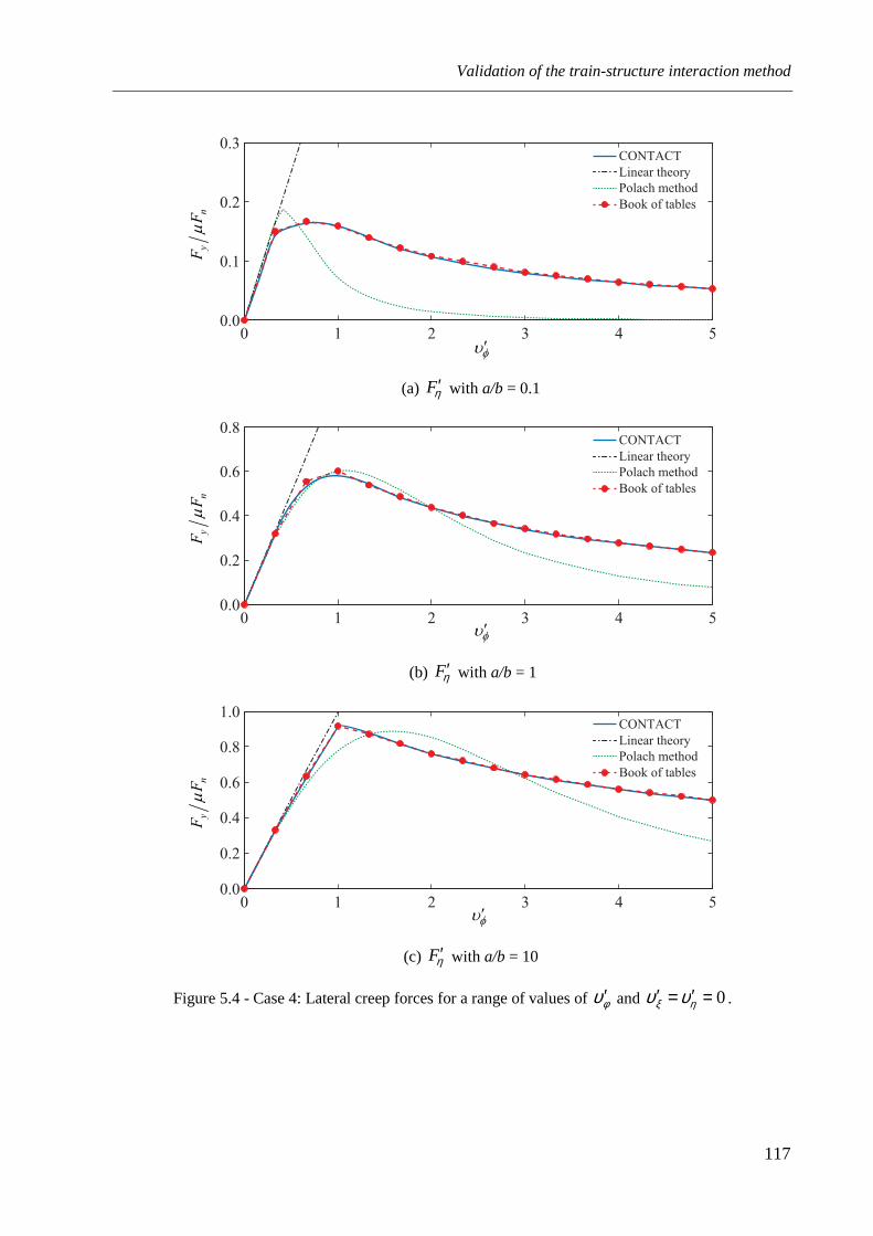
Validation of the train-structure interaction method
117
(a) ηF′ with a/b = 0.1
(b) ηF′ with a/b = 1
(c) ηF′ with a/b = 10
Figure 5.4 - Case 4: Lateral creep forces for a range of values of φυ′ and 0=′=′ ηξ υυ .
0 1 2 3 4 50.0
0.1
0.2
0.3
yn
FF
µ
CONTACT
Linear theory
Polach method
Book of tables
φυ ′
0 1 2 3 4 50.0
0.2
0.4
0.6
0.8
yn
FF
µ
φυ ′
CONTACT
Linear theory
Polach method
Book of tables
0 1 2 3 4 50.0
0.2
0.4
0.6
0.8
1.0
yn
FF
µ
φυ ′
CONTACT
Linear theory
Polach method
Book of tables
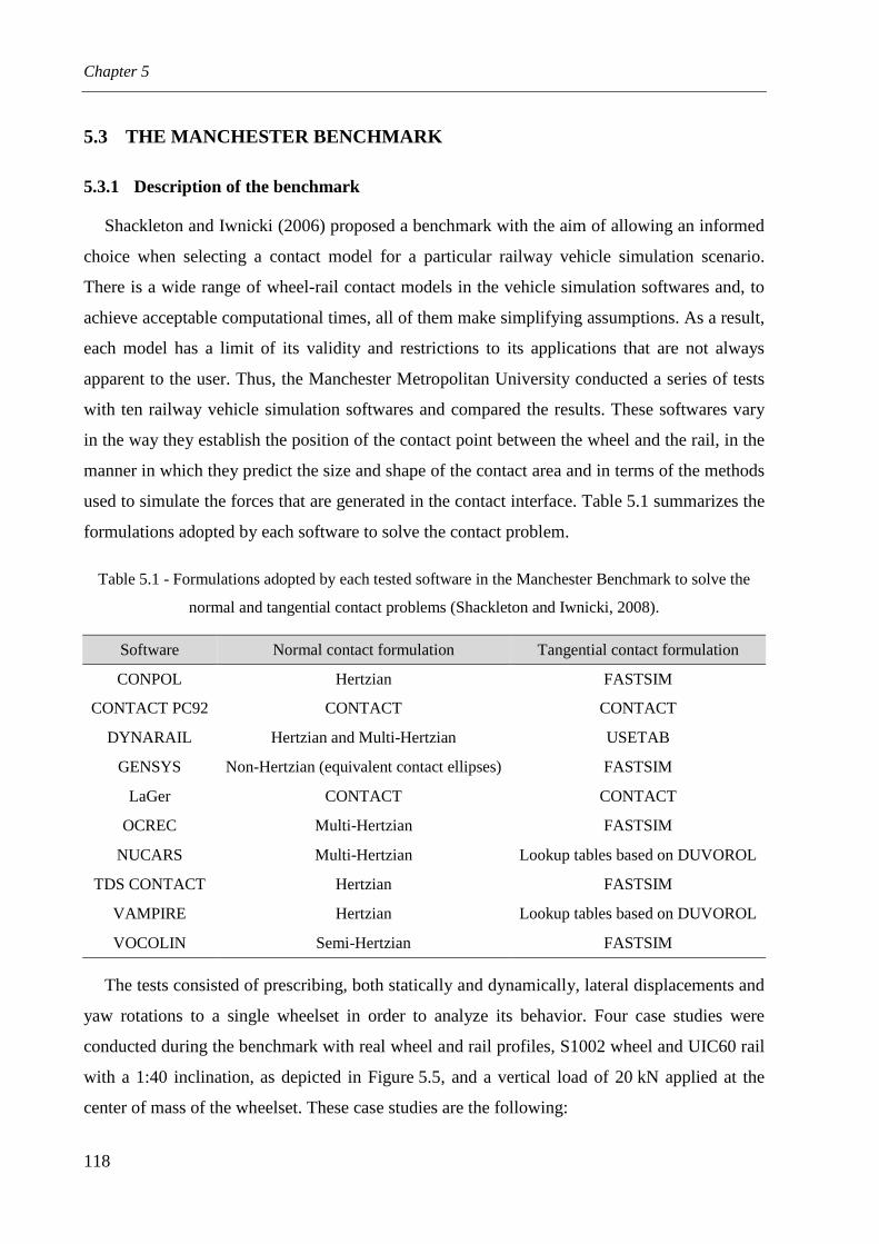
Chapter 5
118
5.3 THE MANCHESTER BENCHMARK
5.3.1 Description of the benchmark
Shackleton and Iwnicki (2006) proposed a benchmark with the aim of allowing an informed
choice when selecting a contact model for a particular railway vehicle simulation scenario.
There is a wide range of wheel-rail contact models in the vehicle simulation softwares and, to
achieve acceptable computational times, all of them make simplifying assumptions. As a result,
each model has a limit of its validity and restrictions to its applications that are not always
apparent to the user. Thus, the Manchester Metropolitan University conducted a series of tests
with ten railway vehicle simulation softwares and compared the results. These softwares vary
in the way they establish the position of the contact point between the wheel and the rail, in the
manner in which they predict the size and shape of the contact area and in terms of the methods
used to simulate the forces that are generated in the contact interface. Table 5.1 summarizes the
formulations adopted by each software to solve the contact problem.
Table 5.1 - Formulations adopted by each tested software in the Manchester Benchmark to solve the
normal and tangential contact problems (Shackleton and Iwnicki, 2008).
Software Normal contact formulation Tangential contact formulation
CONPOL Hertzian FASTSIM
CONTACT PC92 CONTACT CONTACT
DYNARAIL Hertzian and Multi-Hertzian USETAB
GENSYS Non-Hertzian (equivalent contact ellipses) FASTSIM
LaGer CONTACT CONTACT
OCREC Multi-Hertzian FASTSIM
NUCARS Multi-Hertzian Lookup tables based on DUVOROL
TDS CONTACT Hertzian FASTSIM
VAMPIRE Hertzian Lookup tables based on DUVOROL
VOCOLIN Semi-Hertzian FASTSIM
The tests consisted of prescribing, both statically and dynamically, lateral displacements and
yaw rotations to a single wheelset in order to analyze its behavior. Four case studies were
conducted during the benchmark with real wheel and rail profiles, S1002 wheel and UIC60 rail
with a 1:40 inclination, as depicted in Figure 5.5, and a vertical load of 20 kN applied at the
center of mass of the wheelset. These case studies are the following:

Validation of the train-structure interaction method
119
a) Case A1.1: the wheelset is subjected to a prescribed lateral displacement from 0 to
10 mm with 0.5 mm increments. A static analysis is performed in each position and the
normal contact is evaluated;
b) Case A1.2: the wheelset is subjected to the previously described lateral displacements
combined with a yaw rotation from 0 to 24 mrad with 1.2 mrad increments. A static
analysis is performed in each position and the normal contact are evaluated;
c) Case A2.1: forward speed of 2 m.s-1 is given to the wheelset on straight track while it is
subjected to the previously described lateral displacements. A dynamic analysis is
performed and both the normal and tangential contact are evaluated;
d) Case A2.2: the wheelset is subjected to the combinations of lateral displacements and
yaw rotations described in the case A1.2. The dynamic conditions are the same as for
the case A2.1 and both the normal and tangential contact is evaluated.
Figure 5.5 - Wheel and rail profiles used in the benchmark.
5.3.2 Analysis results
The results obtained with the proposed method described in Chapter 4 are compared with
those obtained with the tested softwares. The local coordinate systems considered in the
benchmark, as well as the adopted conventions, are described in Shackleton and Iwnicki (2006)
and in the Appendix B of Shackleton and Iwnicki (2008). Each tested code has been assigned a
line/marker style, being the results obtained with the proposed method superimposed over those
codes.
−80−60−40−200204060−40
−30
−20
−10
0
10
20
y (mm)
z (m
m)
UIC60
RailWheel treadWheel flange
S1002

Chapter 5
120
5.3.2.1 Contact point positions
Figures 5.6 and 5.7 shows the lateral position of the contact point in the rails and wheels,
respectively, defined in the local coordinate systems adopted in the benchmark, for the case
A1.1 and for each wheelset lateral position wsy . The solid line without a marker illustrates the
rail and wheel profile. The proposed method shows a good agreement with the majority of the
tested codes in both the convex and the concave regions of the wheel, validating the contact
search approaches presented in Section 4.3.2 of Chapter 4, respectively.
(a)
(b)
Figure 5.6 - Rail lateral contact positions in case A1.1: (a) left and (b) right rails (adapted from
Shackleton and Iwnicki (2008)).
TDS Contact CONPOL CONTACT PC92 DYNARAIL
GENSYS LaGer NUCARS OCREC
VAMPIRE VOCOLIN ProfileProposed method
−20 −18 −16 −14 −12 −10 −8 −6 −4 −2 0
−2
0
2
4
6
8
10
12
Lateral position (mm)
y ws
(mm
)
−45 −40 −35 −30 −25 −20 −15 −10 −5 0
−2
0
2
4
6
8
10
12
Lateral position (mm)
y ws
(mm
)
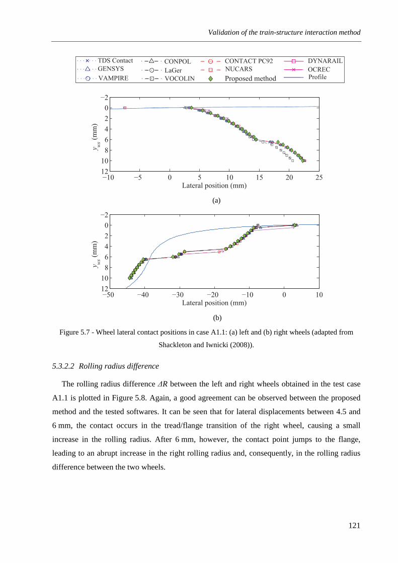
Validation of the train-structure interaction method
121
(a)
(b)
Figure 5.7 - Wheel lateral contact positions in case A1.1: (a) left and (b) right wheels (adapted from
Shackleton and Iwnicki (2008)).
5.3.2.2 Rolling radius difference
The rolling radius difference ∆R between the left and right wheels obtained in the test case
A1.1 is plotted in Figure 5.8. Again, a good agreement can be observed between the proposed
method and the tested softwares. It can be seen that for lateral displacements between 4.5 and
6 mm, the contact occurs in the tread/flange transition of the right wheel, causing a small
increase in the rolling radius. After 6 mm, however, the contact point jumps to the flange,
leading to an abrupt increase in the right rolling radius and, consequently, in the rolling radius
difference between the two wheels.
TDS Contact CONPOL CONTACT PC92 DYNARAIL
GENSYS LaGer NUCARS OCREC
VAMPIRE VOCOLIN ProfileProposed method
−10 −5 0 5 10 15 20 25
−2
0
2
4
6
8
10
12
Lateral position (mm)
y ws
(mm
)
−50 −40 −30 −20 −10 0 10
−2
0
2
4
6
8
10
12
Lateral position (mm)
y ws
(mm
)

Chapter 5
122
Figure 5.8 - Rolling radius difference between right and left wheels in case A1.1 (adapted from
Shackleton and Iwnicki (2008)).
5.3.2.3 Contact angles
Figure 5.9 presents the contact angles in the left lftγ and right rhtγ wheels obtained in the
test case A1.2, in which the lateral displacement of the wheelset is combined with yaw
rotations. The contact angle in the right wheel reaches the maximum value for a lateral
displacement of 6.5 mm accompanied by a yaw rotation of 15.6 mrad and, like the rolling
radius difference, suffers an abrupt increase when the contact point jumps to the flange. The
results obtained with the proposed method for the right contact angle show a good match with
those obtained with all the tested softwares. Regarding the left contact angle, the proposed
method follows the same trend as the softwares GENSYS, NUCARS and VAMPIRE, which
are widely used in railway vehicle simulations. The other two trends are followed by
VOCOLIN and by the softwares LaGer and CONTACT PC92. The discrepancies obtained with
VOCOLIN derive from the non-consideration of the roll rotation of the wheelset to locate the
contact point, while the trend followed by LaGer and CONTACT PC92 is justified by the fact
that the output given by these codes are related to the wheelset coordinate system rather than to
the track centerline coordinate system (see Appendix A for the definition of these coordinate
systems).
0 1 2 3 4 5 6 7 8 9 100
5
10
15
20
25
yws
(mm)
()
mm
R∆
TDS Contact CONPOL CONTACT PC92 DYNARAIL
GENSYS LaGer NUCARS OCREC
VAMPIRE VOCOLIN Proposed method

Validation of the train-structure interaction method
123
(a)
(b)
Figure 5.9 - Contact angle in case A1.2: (a) left and (b) right contact interfaces (adapted from
Shackleton and Iwnicki (2008)).
5.3.2.4 Longitudinal creepages
The longitudinal creepages in the left and right contact interfaces obtained in the dynamic
test case A2.1 are plotted in Figure 5.10. According to Shackleton and Iwnicki (2008), the lack
of conformity between the results predicted by the several codes is due to differences in the
way the total longitudinal creepage is distributed between the left and right contact interfaces.
Therefore, in absolute terms, the output of the proposed method is in agreement with the
outputs obtained with the softwares tested during the benchmark, except CONPOL, which
follows an isolated trend.
TDS Contact CONPOL CONTACT PC92 DYNARAIL
GENSYS LaGer NUCARS OCREC
VAMPIRE VOCOLIN Proposed method
0 1 2 3 4 5 6 7 8 9 100
1
2
3
4γ lf
t (
º)
yws
(mm)
0 1 2 3 4 5 6 7 8 9 100
20
40
60
80
γ rht (
º)
yws
(mm)
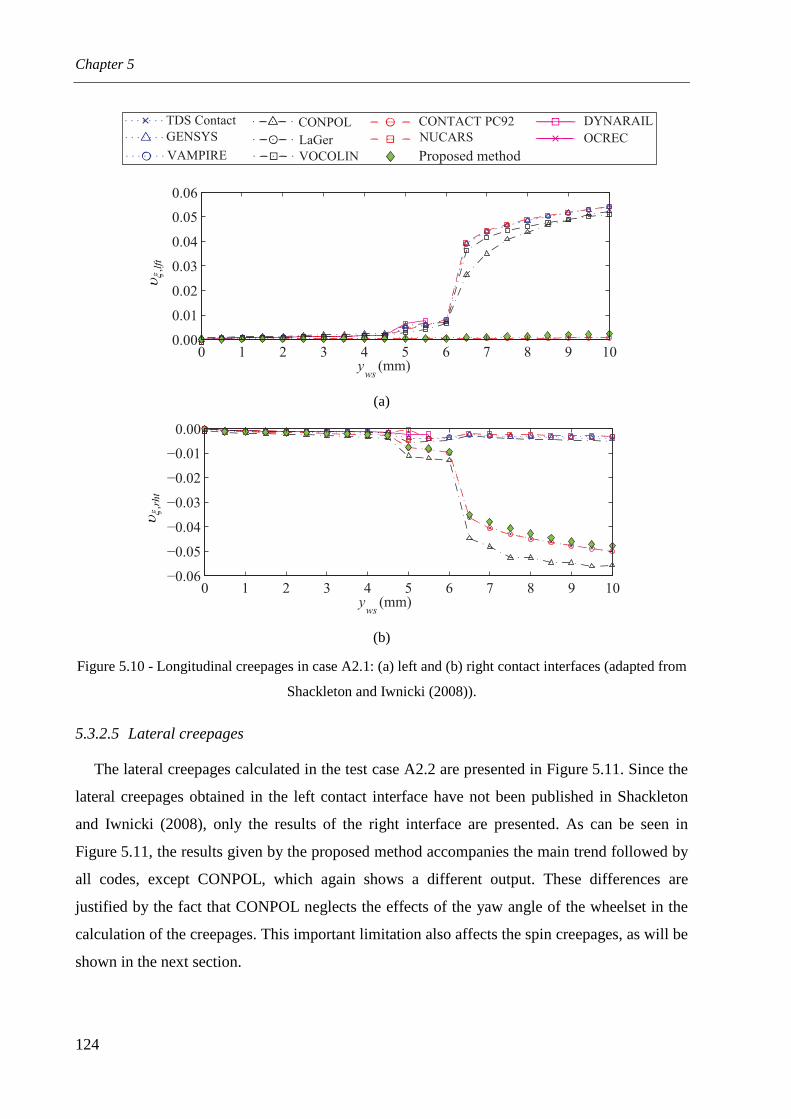
Chapter 5
124
(a)
(b)
Figure 5.10 - Longitudinal creepages in case A2.1: (a) left and (b) right contact interfaces (adapted from
Shackleton and Iwnicki (2008)).
5.3.2.5 Lateral creepages
The lateral creepages calculated in the test case A2.2 are presented in Figure 5.11. Since the
lateral creepages obtained in the left contact interface have not been published in Shackleton
and Iwnicki (2008), only the results of the right interface are presented. As can be seen in
Figure 5.11, the results given by the proposed method accompanies the main trend followed by
all codes, except CONPOL, which again shows a different output. These differences are
justified by the fact that CONPOL neglects the effects of the yaw angle of the wheelset in the
calculation of the creepages. This important limitation also affects the spin creepages, as will be
shown in the next section.
TDS Contact CONPOL CONTACT PC92 DYNARAIL
GENSYS LaGer NUCARS OCREC
VAMPIRE VOCOLIN Proposed method
0 1 2 3 4 5 6 7 8 9 100.00
0.01
0.02
0.03
0.04
0.05
0.06
yws
(mm)
,lft
ξυ
0 1 2 3 4 5 6 7 8 9 10−0.06
−0.05
−0.04
−0.03
−0.02
−0.01
0.00
yws (mm)
,rht
ξυ

Validation of the train-structure interaction method
125
Figure 5.11 - Lateral creepages at the right contact interface in case A2.2 (adapted from Shackleton and
Iwnicki (2008)).
5.3.2.6 Spin creepages
Finally, the spin creepages in the left and right contact interfaces obtained in the test case
A2.2 are plotted in Figure 5.12. The spin creepages follows the same trend as the contact angle
(see Figure 5.9), since they depend directly on it. Therefore, the different trends observed in the
left side are justified by the same reasons presented in Section 5.3.2.3, while the discrepancies
obtained with CONPOL in the right side are, once more, due to the non-consideration of the
yaw angle effects in the calculation of the creepages.
Regarding the proposed method, a good agreement is observed between the results obtained
with it in the right contact interface and those obtained with the softwares tested during the
benchmark, with exception to CONPOL for the reasons stated above. In the left side, the
proposed method follows again the same trend as GENSYS and VAMPIRE.
4 5 6 7 8 9 10−0.05
−0.04
−0.03
−0.02
−0.01
yws (mm)
,rh
tη
υ
TDS Contact CONPOL CONTACT PC92 DYNARAIL
GENSYS LaGer NUCARS OCREC
VAMPIRE VOCOLIN Proposed method

Chapter 5
126
(a)
(b)
Figure 5.12 - Spin creepages in case A2.2: (a) left and (b) right contact interfaces (adapted from
Shackleton and Iwnicki (2008)).
5.3.2.7 Conclusions
Although a general agreement between the tested softwares and the proposed method is
observed, there are, in some cases, notable discrepancies. However, the main discrepancies are
mainly justified by limitations of the contact models adopted by some of the tested softwares,
especially CONPOL and VOCOLIN, rather than by limitations of the proposed method.
Moreover, the results obtained with the proposed method are, in most cases, in an excellent
agreement with those obtained with GENSYS, NUCARS and VAMPIRE, which are widely
used in dynamic simulations of railway vehicles. Therefore, it can be concluded that the
wheel-rail contact model developed in this work is suitable for being used in railway dynamics
applications.
TDS Contact CONPOL CONTACT PC92 DYNARAIL
GENSYS LaGer NUCARS OCREC
VAMPIRE VOCOLIN Proposed method
0 1 2 3 4 5 6 7 8 9 100.00
0.01
0.02
0.03
0.04
0.05
0.06
yws
(mm)
()
,ra
dm
lft
φυ
0 1 2 3 4 5 6 7 8 9 100.0
0.5
1.0
1.5
2.0
2.5
yws
(mm)
()
,ra
dm
rht
φυ

Validation of the train-structure interaction method
127
5.4 HUNTING STABILITY ANALYSIS OF A SUSPENDED WHEELSET
5.4.1 The hunting phenomenon
Due to the specific conic shape of the train wheels, when a wheelset is running on a straight
track and is subjected to a lateral perturbation, the rolling radii of the left and right wheel differ
from each other. Hence, since both wheels have the same angular velocity if the wheelset is
running with a constant speed, the wheel with larger radius will experiment a higher velocity
than the opposite wheel. This phenomenon will force the wheelset to yaw and go back to the
centered position, making the rolling radius of the opposite wheel to become larger. This
process, called hunting motion (see Figure 5.13), tends to continue indefinitely in an
unsuspended wheelset making it unstable (Garg and Dukkipati, 1984; Andersson et al., 1999;
Wickens, 2003). However, the creep forces that arise in the contact interface act as damping
forces that dissipate energy and ensure the existence of a certain range of speeds where the
wheelset is stable. The speed above which the wheelset become unstable is called critical
speed. In addition to the creep forces, the critical speed of a wheelset also depends on the wheel
conicity, wheelset mechanical properties and suspensions. The last one is particularly important
to ensure that the wheelset instability occurs only at higher ranges of speeds.
Figure 5.13 - Schematic representation of the hunting motion.
When a wheelset experiences the hunting motion, its center of gravity follows an almost
sinusoidal lateral motion around the track centerline, as illustrated in Figure 5.13. Klingel
(1883) was the first author to derive an expression which describes this motion on a
non-suspended wheelset. Based on purely kinematic relationships, Klingel proposed the
following expression for the wavelength Klingelλ of the hunting motion:
0
02γ
πλRLcp
Klingel = (5.1)
Sinusoidal
motion
track centerline

Chapter 5
128
where 0R the initial rolling radius of the wheel, Lcp is the half lateral distance between contact
points and 0γ is the conicity of the wheels. However, as aforementioned, this expression only
considers the kinematic components of the movement, ignoring the inertial effects due to the
mass of the wheelset, the influence of the suspensions flexibility, the creep forces that arise in
the contact interface and the real shape of the wheels (the wheels are perfectly conical in the
Klingel's model). Hence, in order to allow a reliable validation of the proposed method, a fully
dynamic model of the wheelset is adopted.
5.4.2 Numerical model
The numerical model consists of a single suspended wheelset connected to a moving frame
by lateral and longitudinal suspensions, as shown in Figure 5.14.
Figure 5.14 - Dynamic model of a suspended wheelset connected to a moving frame (top view).
The geometrical and mechanical properties of the model, which are based on those defined
by Valtorta et al. (2001), are presented in Table 5.2. Note that the contact ellipse semi-axes a
and b, as well as the Kalker creepage coefficients 11c and 22c , are calculated for a static position
of the wheelset centered with the track and maintained constant throughout the analysis.
2L
l
1
wsy
wsxws
ψ
0R
1, 1,,y yk c
1, 1,,x xk c
0γcp
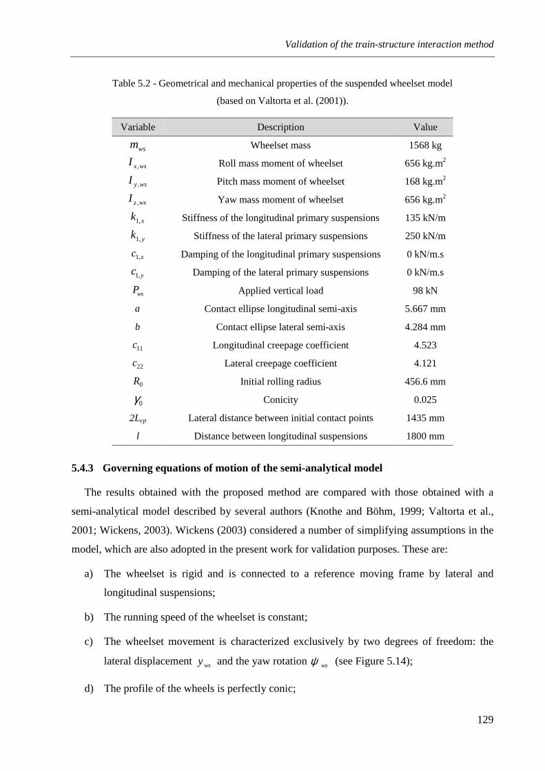
Validation of the train-structure interaction method
129
Table 5.2 - Geometrical and mechanical properties of the suspended wheelset model
(based on Valtorta et al. (2001)).
Variable Description Value
wsm Wheelset mass 1568 kg
wsxI , Roll mass moment of wheelset 656 kg.m2
wsyI , Pitch mass moment of wheelset 168 kg.m2
wszI , Yaw mass moment of wheelset 656 kg.m2
xk ,1 Stiffness of the longitudinal primary suspensions 135 kN/m
yk ,1 Stiffness of the lateral primary suspensions 250 kN/m
xc ,1 Damping of the longitudinal primary suspensions 0 kN/m.s
yc ,1 Damping of the lateral primary suspensions 0 kN/m.s
wsP Applied vertical load 98 kN
a Contact ellipse longitudinal semi-axis 5.667 mm
b Contact ellipse lateral semi-axis 4.284 mm
11c Longitudinal creepage coefficient 4.523
22c Lateral creepage coefficient 4.121
0R Initial rolling radius 456.6 mm
0γ Conicity 0.025
2Lcp Lateral distance between initial contact points 1435 mm
l Distance between longitudinal suspensions 1800 mm
5.4.3 Governing equations of motion of the semi-analytical model
The results obtained with the proposed method are compared with those obtained with a
semi-analytical model described by several authors (Knothe and Böhm, 1999; Valtorta et al.,
2001; Wickens, 2003). Wickens (2003) considered a number of simplifying assumptions in the
model, which are also adopted in the present work for validation purposes. These are:
a) The wheelset is rigid and is connected to a reference moving frame by lateral and
longitudinal suspensions;
b) The running speed of the wheelset is constant;
c) The wheelset movement is characterized exclusively by two degrees of freedom: the
lateral displacement wsy and the yaw rotation wsψ (see Figure 5.14);
d) The profile of the wheels is perfectly conic;
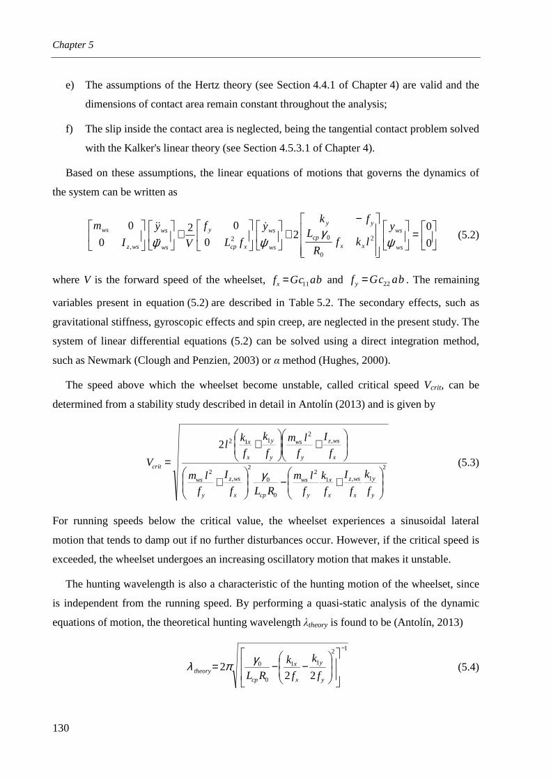
Chapter 5
130
e) The assumptions of the Hertz theory (see Section 4.4.1 of Chapter 4) are valid and the
dimensions of contact area remain constant throughout the analysis;
f) The slip inside the contact area is neglected, being the tangential contact problem solved
with the Kalker's linear theory (see Section 4.5.3.1 of Chapter 4).
Based on these assumptions, the linear equations of motions that governs the dynamics of
the system can be written as
=
−+
+
0
02
0
020
02
0
02, ws
ws
xxcp
yy
ws
ws
xcp
y
ws
ws
wsz
ws y
lkfR
Lfk
y
fL
f
V
y
I
m
ψγ
ψψ ɺ
ɺ
ɺɺ
ɺɺ
(5.2)
where V is the forward speed of the wheelset, bacGfx 11= and bacGfy 22= . The remaining
variables present in equation (5.2) are described in Table 5.2. The secondary effects, such as
gravitational stiffness, gyroscopic effects and spin creep, are neglected in the present study. The
system of linear differential equations (5.2) can be solved using a direct integration method,
such as Newmark (Clough and Penzien, 2003) or α method (Hughes, 2000).
The speed above which the wheelset become unstable, called critical speed Vcrit, can be
determined from a stability study described in detail in Antolín (2013) and is given by
2
1,12
0
0
2
,2
,2
1122
+−
+
+
+
=
y
y
x
wsz
x
x
y
ws
cpx
wsz
y
ws
x
wsz
y
ws
y
y
x
x
crit
f
k
f
I
f
k
f
lm
RLf
I
f
lm
f
I
f
lm
f
k
f
kl
Vγ
(5.3)
For running speeds below the critical value, the wheelset experiences a sinusoidal lateral
motion that tends to damp out if no further disturbances occur. However, if the critical speed is
exceeded, the wheelset undergoes an increasing oscillatory motion that makes it unstable.
The hunting wavelength is also a characteristic of the hunting motion of the wheelset, since
is independent from the running speed. By performing a quasi-static analysis of the dynamic
equations of motion, the theoretical hunting wavelength λtheory is found to be (Antolín, 2013)
12
11
0
0
222
−
−−=
y
y
x
x
cptheory f
k
f
k
RL
γπλ (5.4)

Validation of the train-structure interaction method
131
Notice that the theoretical hunting wavelength expressed in equation (5.4) becomes equal to
the wavelength proposed by Klingel, defined in equation (5.1), if the dynamic terms are
neglected.
5.4.4 Analysis results
The results obtained with the numerical integration of the system of equations (5.2) are
compared with those obtained with the proposed train-structure interaction method described in
Chapter 4. The time step used in all the analysis with both the numerical and semi-analytical
models is s001.0=∆t and the total number of time steps is 8000. The Newmark integration
scheme (Clough and Penzien, 2003) with integration parameters α = 0, β = 0.25 and γ = 0.5 is
used to solve the equations of motion. At the beginning of the dynamic analysis, a lateral
impulsive load of 100 N is applied at the center of mass of the wheelset in order to drive the
system away from its equilibrium position, causing it to oscillate over the track centerline.
Since the equations that govern the dynamic behavior of the analytic model are based on the
assumption that there is no slip inside the contact area (see equation (5.2)), the Kalker's linear
model is adopted to compute the creep forces in the simulations performed in the present
section.
For the wheelset considered in the present problem, the critical speed calculated with
equation (5.3) is Vcrit = 234.4 km/h. Thus, the response of the wheelset when it is running at a
speed below and above the critical value is evaluated. Figures 5.15 and 5.16 show the
comparison between the responses of the wheelset obtained with the proposed method and with
the semi-analytical equations of motion expressed by equation (5.2), for a running speed of
100 km/h and 250 km/h, respectively. The results obtained with both formulations show a good
agreement, with slight differences observed in the solution regarding the wheelset running
above the critical speed. These differences may be justified by the fact that the numerical model
accounts for a minimum flexibility to avoid numerical instabilities, since it is developed in a
finite element method framework. As expected, when the wheelset runs below the critical
speed, the energy dissipation due to the creep forces and the stability provided by the primary
suspensions lead to a decrement of the hunting amplitude. On the other hand, when the
wheelset travels at 250 km/h the behavior becomes unstable and the system does not return to
the centered position.
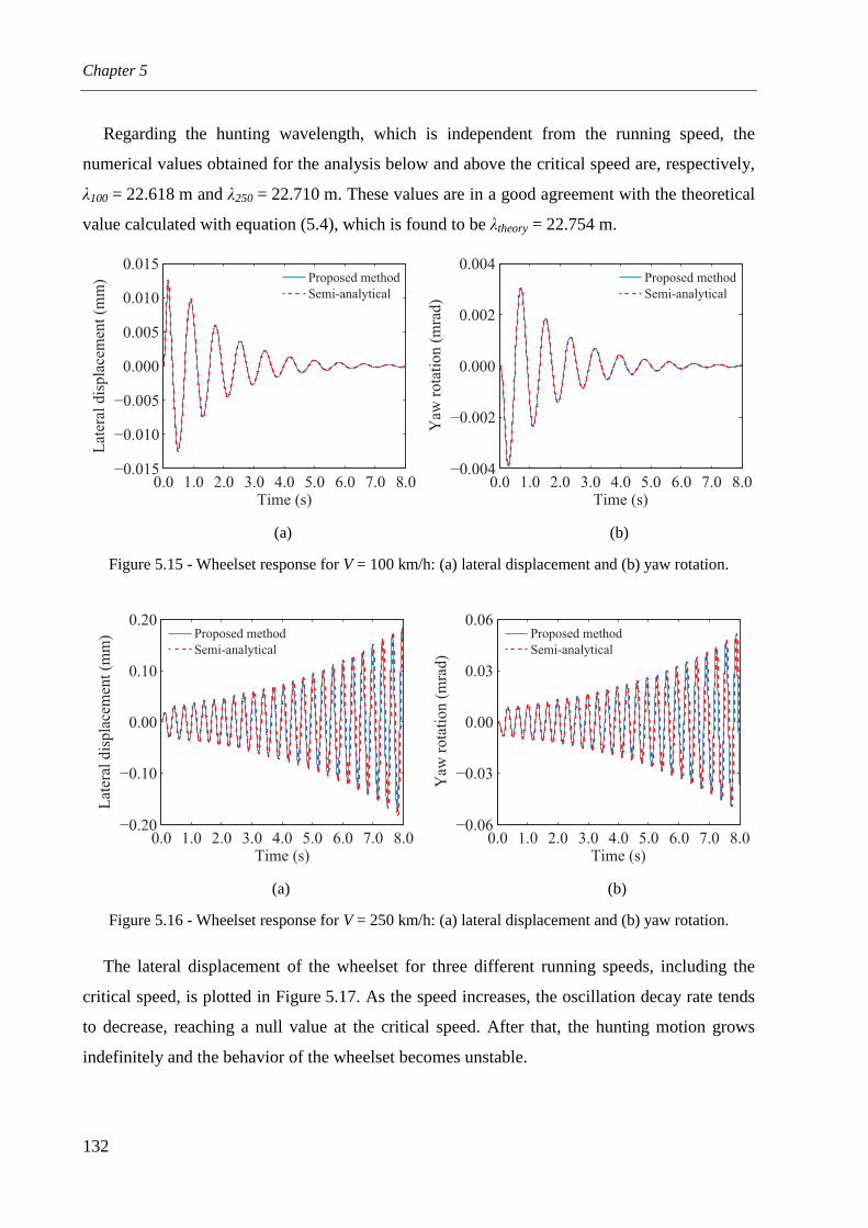
Chapter 5
132
Regarding the hunting wavelength, which is independent from the running speed, the
numerical values obtained for the analysis below and above the critical speed are, respectively,
λ100 = 22.618 m and λ250 = 22.710 m. These values are in a good agreement with the theoretical
value calculated with equation (5.4), which is found to be λtheory = 22.754 m.
(a) (b)
Figure 5.15 - Wheelset response for V = 100 km/h: (a) lateral displacement and (b) yaw rotation.
(a) (b)
Figure 5.16 - Wheelset response for V = 250 km/h: (a) lateral displacement and (b) yaw rotation.
The lateral displacement of the wheelset for three different running speeds, including the
critical speed, is plotted in Figure 5.17. As the speed increases, the oscillation decay rate tends
to decrease, reaching a null value at the critical speed. After that, the hunting motion grows
indefinitely and the behavior of the wheelset becomes unstable.
0.0 1.0 2.0 3.0 4.0 5.0 6.0 7.0 8.0−0.015
−0.010
−0.005
0.000
0.005
0.010
0.015
Time (s)
Lateral displacement (mm) Proposed method
Semi-analytical
0.0 1.0 2.0 3.0 4.0 5.0 6.0 7.0 8.0−0.004
−0.002
0.000
0.002
0.004
Time (s)
Yaw
rotation (mrad)
Proposed method
Semi-analytical
0.0 1.0 2.0 3.0 4.0 5.0 6.0 7.0 8.0−0.20
−0.10
0.00
0.10
0.20
Time (s)
Lateral displacement (mm) Proposed method
Semi-analytical
0.0 1.0 2.0 3.0 4.0 5.0 6.0 7.0 8.0−0.06
−0.03
0.00
0.03
0.06
Time (s)
Yaw
rotation (mrad)
Proposed method
Semi-analytical

Validation of the train-structure interaction method
133
Figure 5.17 - Wheelset lateral displacement for three different running speeds.
The critical speed is therefore a transition in the dynamic behavior of the wheelset that can
be analyzed with the logarithmic decrement factor nδ , given by
( )
( )
+=
Tnty
ty
n ws
wsn ln
1δ (5.5)
where ( )tyws and ( )Tntyws + are two peak displacements separated by n consecutive cycles with
period T. The logarithmic decrement related to the responses of the wheelset for speeds ranging
from 50 km/h to 300 km/h is depicted in Figure 5.18. As expected, the logarithmic decrement
for the lower speeds is positive, but starts to decrease as the speed increases. Once the critical
speed is reached, the decrement becomes null, since the hunting motion maintains the
amplitude throughout the analysis, as shown in Figure 5.17. Then, once the speed exceeds the
critical value, the decrement turns negative and the wheelset experiences an unstable behavior.
Figure 5.18 - Logarithmic decrement factor as a function of the wheelset speed.
0.0 1.0 2.0 3.0 4.0−0.10
−0.05
0.00
0.05
0.10
Time (s)
Lateral displacement (mm)
V = 200 km/h
V = 250 km/h
V = Vcrit
0 50 100 150 200 250 300−0.2
−0.1
0.0
0.1
0.2
0.3
Speed (km/h)
Logarithmic decrement
Criticalspeed
235km
h≃
null decrement

Chapter 5
134
5.5 SIMULATION OF AN EXPERIMENTAL TEST CONDUCTED IN A
ROLLING STOCK TEST PLANT
5.5.1 Background and description of the experimental test
High-speed railway lines require a more rigorous maintenance when compared with
conventional lines. Since the displacements of the structures may contribute to significant track
deviations, and subsequently influence the riding comfort or the running safety of the train,
deflection limits should be imposed during the design of railway structures. Such precautions
are particularly important in countries prone to earthquakes, where large lateral displacements
may occur during a seismic event. Japan, with one of the largest railway networks in the world,
is one of those countries. Hence, in November 2000, the Committee on Displacement Limit of
Structures Associated with the Runnability of Railway Vehicles, consisting of engineers and
academics specialized in the design of railway structures and in the study of vehicle dynamics,
was formed to draw a Displacement Limit Standard for Railway Structures.
Over three years, the committee draft the code provisions based on results obtained in a
series of experimental tests, developed in shaking tables and rolling stock test plants using full
scale test vehicles, and in numerical simulations regarding the running safety of trains. Finally,
in April 2004, the committee approved the final code provision. However, due to the 2004
Mid-Niigata Earthquake that occurred on October 2004, in which a Shinkansen train derailed
when running over a bridge at 200 km/h, the publication of the code was postponed, since it
also included provisions regarding the running safety of trains under seismic conditions. After
taking into consideration a report drawn by the Shinkansen Derailing Countermeasures
Council, the Displacement Limit Standard for Railway Structures (RTRI, 2006) was finally
published at the beginning of 2006.
One of the experimental tests (Sogabe et al., 2006) used to draft the Displacement Limit
Standard is numerically reproduced in the present section (Montenegro et al., 2015b). The test
was conducted in the rolling stock test plant in the RTRI and consisted in the analysis of a
railway vehicle mounted over a test rig with four wheel-shaped rails controlled by independent
actuators that can simulate different types of rail deviations (see Figure 5.19).

Validation of the train-structure interaction method
135
(a) (b)
Figure 5.19 - Experimental test: (a) rolling stock test plant (RTRI, 2013) and (b) test setup (adapted
from Sogabe et al. (2005)).
Both vertical and lateral deviations were imposed to the track while the vehicle ran over it.
These deviations aimed to simulate track misalignments caused by the deflection of a bridge
when it is subjected to an earthquake. When these situations occur, the vehicle may experience
high levels of vibrations while travelling over the bridge, leading to an increased risk of
derailment. The deflection types considered in the test are divided into two: a bending shape
(BS), associated with the bending of two consecutive spans, and a translation shape (TS), in
which only one span rotates while the other is subjected to a translation, as illustrated in
Figure 5.20. Span lengths L ranging from 10 m to 60 m were also considered in the tests,
together with transition sections at the ends of each span to guarantee a smooth continuity of
rotations of the rail (see Figure 5.20c).
Figure 5.20 - Deflection models: (a) BS, (b) TS and (c) detail of the transition.
During the tests, the vertical and lateral accelerations of the carbody were measured above
the rear bogie. The tests were conducted with a full scale railway vehicle running over the test
stand at speeds ranging from 100 to 400 km/h. The maximum deflection amplitude considered
in all scenarios was δ = 8 mm (see Figure 5.20) for both the vertical and lateral directions.
Primary suspensions
Measurement point
of accelerationCarbody
Actuator for
vertical vibration
Driving device
Wheel-shaped rail
Actuator for
lateral vibration
Wheelset
Bogie
Secondary suspensions
L L
tL tL
δ
tθL
tL tL
tθ
t
δ
θ
(a) (b) (c)
Structure
Rail smoothing
Track stiffness
tL tL
tθtytx
L

Chapter 5
136
5.5.2 Numerical model
5.5.2.1 Structure model
The structure shown in Figure 5.20 is modeled with rigid finite elements, being the track
deviation introduced as irregularities in the vertical and lateral directions. The half length of the
transition zone is denoted by Lt (see Figure 5.20c), the span rotation by θt and the distance from
the start of the transition zone by xt. This procedure avoids numerical problems associated with
unrealistic impacts that may occur in abrupt transitions. Thus, according to Sogabe et al. (2005;
2006), the track deviation yt in the transition is given by
( ) ( )[ ] ( )[ ]
( ) ( )[ ] ( )[ ] ( )
≤<−+−+−
≤≤−+−=
−−
−
ttttttttttttLtxt
t
t
tttttttttLtxt
t
t
t
LxLLxLxLxe
LxLxLxe
y2ifsincos
4
0ifsincos4
θβββ
θ
βββ
θ
β
β
(5.6)
where βt is the relative bending stiffness of the rails and pads in the lateral direction, given by
4
4 r
pt IE
k=β (5.7)
where kp is the pad stiffness, E the Young modulus of the steel and Ir the moment of inertia of
the rail. The parameters used for defining the transition zones are summarized in Table 5.3.
Table 5.3 - Parameters of the transition zones.
Variable Track direction
Vertical Lateral
tL 3 m 3 m
pk
9.4× 10⁴ kN/m/m 47.1× 10⁴ kN/m/m
rI 3090 cm4 509 cm4
5.5.2.2 Vehicle model
The test vehicle consists of a narrow gauge prototype car specially developed for the
experimental test, whose properties were provided by the RTRI1. A schematic representation
of the dynamic model of the test vehicle is illustrated in Figure 5.21. The springs and dampers
of the suspensions are denoted by k and c and the masses and rotary inertias are indicated by m
1 The geometrical and mechanical properties of the test vehicle are not published due to confidential matters from the manufacturer.
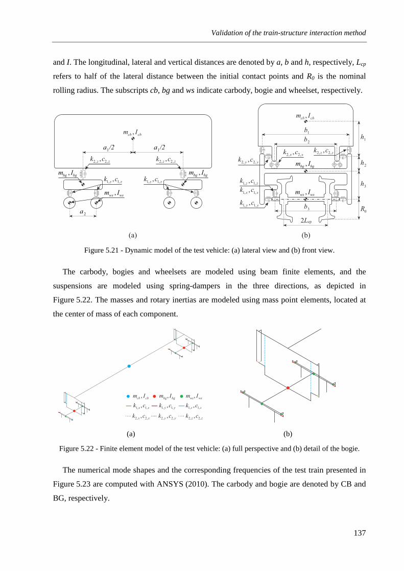
Validation of the train-structure interaction method
137
and I. The longitudinal, lateral and vertical distances are denoted by a, b and h, respectively, Lcp
refers to half of the lateral distance between the initial contact points and R0 is the nominal
rolling radius. The subscripts cb, bg and ws indicate carbody, bogie and wheelset, respectively.
Figure 5.21 - Dynamic model of the test vehicle: (a) lateral view and (b) front view.
The carbody, bogies and wheelsets are modeled using beam finite elements, and the
suspensions are modeled using spring-dampers in the three directions, as depicted in
Figure 5.22. The masses and rotary inertias are modeled using mass point elements, located at
the center of mass of each component.
(a) (b)
Figure 5.22 - Finite element model of the test vehicle: (a) full perspective and (b) detail of the bogie.
The numerical mode shapes and the corresponding frequencies of the test train presented in
Figure 5.23 are computed with ANSYS (2010). The carbody and bogie are denoted by CB and
BG, respectively.
1, 1,,y yk c
1, 1,,x xk c1, 1,,z zk c
2, 2,,z zk c
2, 2,,y yk c2, 2,,x xk c
1h
2h
3h
0R
1b
2b
3b
,cb cbm I
(a) (b)
,cb cbm I
2, 2,,z zk c
1a /2
2, 2,,z zk c
2a
1, 1,,z zk c1, 1,,z zk c
1a /2
2Lcp
,ws wsm I ,ws wsm I
,bg bgm I
,bg bgm I,bg bgm I
,cb cbm I
1, 1,,x xk c
1, 1,,y yk c 1, 1,,z zk c
2, 2,,z zk c2, 2,,y yk c2, 2,,x xk c
,bg bgm I ,ws wsm I
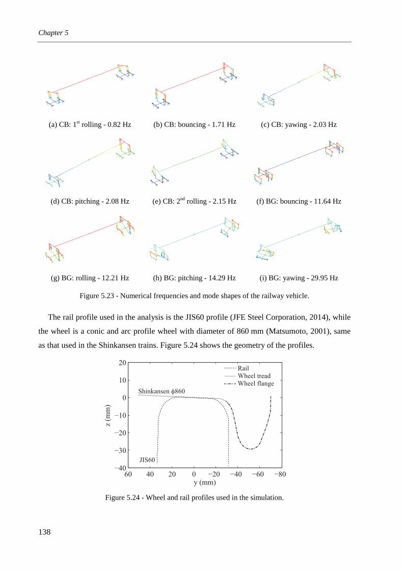
Chapter 5
138
(a) CB: 1st rolling - 0.82 Hz (b) CB: bouncing - 1.71 Hz (c) CB: yawing - 2.03 Hz
(d) CB: pitching - 2.08 Hz (e) CB: 2nd rolling - 2.15 Hz (f) BG: bouncing - 11.64 Hz
(g) BG: rolling - 12.21 Hz (h) BG: pitching - 14.29 Hz (i) BG: yawing - 29.95 Hz
Figure 5.23 - Numerical frequencies and mode shapes of the railway vehicle.
The rail profile used in the analysis is the JIS60 profile (JFE Steel Corporation, 2014), while
the wheel is a conic and arc profile wheel with diameter of 860 mm (Matsumoto, 2001), same
as that used in the Shinkansen trains. Figure 5.24 shows the geometry of the profiles.
Figure 5.24 - Wheel and rail profiles used in the simulation.
−80−60−40−200204060−40
−30
−20
−10
0
10
20
y (mm)
z (m
m)
RailWheel treadWheel flange
JIS60
Shinkansen φ860

Validation of the train-structure interaction method
139
5.5.3 Analysis results
The results obtained with the train-structure interaction method described in Chapter 4 are
compared with those obtained in the experimental test and with DIASTARS. The time step
used in all the performed analysis is s001.0=∆t and the total number of time steps is 2500.
Since DIASTARS uses the Newmark integration scheme (Clough and Penzien, 2003) to solve
the equations of motion, no numerical dissipation is considered in the α method in order to
establish a more reliable comparison. Therefore, the integration parameters α = 0, β = 0.25 and
γ = 0.5 are adopted. All the results presented in this section regarding the vertical direction are
obtained exclusively with the imposition of vertical deflections to the track, while the results
relative to the lateral direction are obtained with the imposition of transversal deflections (see
Section 5.5.1).
The comparison between the vertical accelerations measured in the carbody above the rear
bogie and the results obtained with the proposed method and DIASTARS is depicted in
Figure 5.25. The same comparison, but for the lateral accelerations measured at the same point,
is plotted in Figure 5.26. The results shown on both figures correspond to an analysis in which
the vehicle is running at V = 300 km/h and the letters y and z presented in the deflection
schemes of those figures indicate lateral and vertical deflection shapes, respectively. A good
agreement can be observed between the measured data and the numerical results. The
differences observed may be justified by the fact that the numerical model of the vehicle does
not consider the flexibility of some components, especially the carbody, where the
accelerations were measured. The lack of additional experimental data to calibrate the vehicle
model may also contribute to these differences. When comparing the numerical results obtained
with the proposed method and with DIASTARS an excellent agreement can be observed. The
slight differences may be due to the fact that the two numerical formulations are based on
different wheel-rail contact models. The DIASTARS uses an offline contact search algorithm
and a creep model based on Kalker's linear theory with a saturation limit for high creepages,
whereas the proposed method uses an online contact search formulation and the Kalker's book
of tables to compute the creep forces.

Chapter 5
140
(a)
(b)
(c)
(d)
Figure 5.25 - Vertical accelerations in the carbody above the rear bogie for V = 300 km/h: (a) BS - 20 m
span; (b) BS - 40 m span; (c) TS - 20 m span; (d) TS - 40 m span.
0.0 0.5 1.0 1.5 2.0 2.5−1.5
−1.0
−0.5
0.0
0.5
1.0
1.5
2.0
Time (s)
Vertical accel. (m.s−2)
Proposed method
DIASTARS
Experimental
z
0.0 0.5 1.0 1.5 2.0 2.5−0.4
−0.2
0.0
0.2
0.4
0.6
Time (s)
Vertical accel. (m.s−2)
Proposed method
DIASTARS
Experimental
z
0.0 0.5 1.0 1.5 2.0 2.5−0.8
−0.4
0.0
0.4
0.8
1.2
Time (s)
Vertical accel. (m.s−2)
Proposed method
DIASTARS
Experimental
z
0.0 0.5 1.0 1.5 2.0 2.5−0.3
−0.2
−0.1
0.0
0.1
0.2
0.3
0.4
Time (s)
Vertical accel. (m.s−2)
Proposed method
DIASTARS
Experimental
z

Validation of the train-structure interaction method
141
(a)
(b)
(c)
(d)
Figure 5.26 - Lateral accelerations in the carbody above the rear bogie for V = 300 km/h: (a) BS - 40 m
span; (b) BS - 20 m span; (c) TS - 40 m span; (d) TS - 20 m span.
0.0 0.5 1.0 1.5 2.0 2.5−1.0
−0.5
0.0
0.5
1.0
1.5
Time (s)
Lateral accel. (m.s−2)
Proposed method
DIASTARS
Experimental
y
0.0 0.5 1.0 1.5 2.0 2.5−0.4
−0.2
0.0
0.2
0.4
0.6
0.8
Time (s)
Lateral accel. (m.s−2)
Proposed method
DIASTARS
Experimental
y
0.0 0.5 1.0 1.5 2.0 2.5−0.6
−0.4
−0.2
0.0
0.2
0.4
0.6
0.8
Time (s)
Lateral accel. (m.s−2)
Proposed method
DIASTARS
Experimental
y
0.0 0.5 1.0 1.5 2.0 2.5−0.4
−0.2
0.0
0.2
0.4
Time (s)
Lateral accel. (m.s−2)
Proposed method
DIASTARS
Experimental
y

Chapter 5
142
Figures 5.27 and 5.28 show, respectively, the maximum vertical and lateral accelerations in
the carbody, obtained in the experimental tests and with the proposed method. The results refer
to span lengths of 10, 20, 40 and 60 m and vehicle speeds ranging from 100 km/h to 400 km/h
with steps of 50 km/h. In most of the cases, the numerical results show a good agreement with
the experimental results. Some discrepancies may be justified by the incapacity of the actuators
to reproduce with precision the track rotations (Sogabe et al., 2006).
(a) (b)
Figure 5.27 - Maximum vertical accelerations in the carbody above rear bogie: (a) BS and (b) TS tests.
(a) (b)
Figure 5.28 - Maximum lateral accelerations in the carbody above rear bogie: (a) BS and (b) TS tests.
Proposed method:
Experimental: L=10 m
L=10 m
L=20 m
L=20 m
L=40 m
L=40 m
L=60 m
L=60 m
0 100 200 300 4000.0
0.5
1.0
1.5
2.0
Velocity (km/h)
Ver
tica
l ac
cele
rati
on (
m.s
−2 ) z
0 100 200 300 4000.0
0.5
1.0
1.5
2.0
Velocity (km/h)
Ver
tica
l ac
cele
rati
on
(m
.s −
2 ) z
Proposed method:
Experimental: L=10 m
L=10 m
L=20 m
L=20 m
L=40 m
L=40 m
L=60 m
L=60 m
0 100 200 300 4000.0
0.5
1.0
1.5
Velocity (km/h)
Lat
eral
acc
eler
atio
n (
m.s
−2)
y
0 100 200 300 4000.0
0.5
1.0
1.5
Velocity (km/h)
Lat
eral
acc
eler
atio
n (
m.s
−2)
y
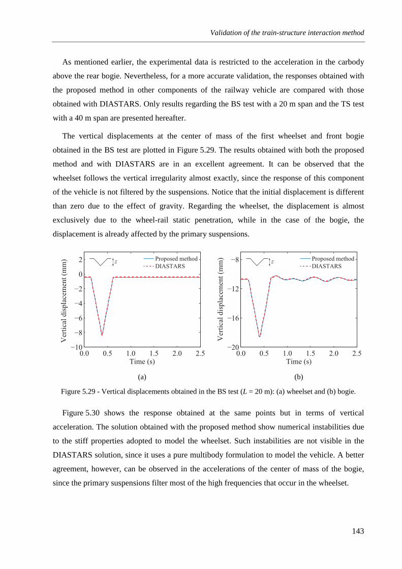
Validation of the train-structure interaction method
143
As mentioned earlier, the experimental data is restricted to the acceleration in the carbody
above the rear bogie. Nevertheless, for a more accurate validation, the responses obtained with
the proposed method in other components of the railway vehicle are compared with those
obtained with DIASTARS. Only results regarding the BS test with a 20 m span and the TS test
with a 40 m span are presented hereafter.
The vertical displacements at the center of mass of the first wheelset and front bogie
obtained in the BS test are plotted in Figure 5.29. The results obtained with both the proposed
method and with DIASTARS are in an excellent agreement. It can be observed that the
wheelset follows the vertical irregularity almost exactly, since the response of this component
of the vehicle is not filtered by the suspensions. Notice that the initial displacement is different
than zero due to the effect of gravity. Regarding the wheelset, the displacement is almost
exclusively due to the wheel-rail static penetration, while in the case of the bogie, the
displacement is already affected by the primary suspensions.
(a) (b)
Figure 5.29 - Vertical displacements obtained in the BS test (L = 20 m): (a) wheelset and (b) bogie.
Figure 5.30 shows the response obtained at the same points but in terms of vertical
acceleration. The solution obtained with the proposed method show numerical instabilities due
to the stiff properties adopted to model the wheelset. Such instabilities are not visible in the
DIASTARS solution, since it uses a pure multibody formulation to model the vehicle. A better
agreement, however, can be observed in the accelerations of the center of mass of the bogie,
since the primary suspensions filter most of the high frequencies that occur in the wheelset.
0.0 0.5 1.0 1.5 2.0 2.5−10
−8
−6
−4
−2
0
2
Time (s)
Vertical displacement (mm) Proposed method
DIASTARSz
0.0 0.5 1.0 1.5 2.0 2.5−20
−16
−12
−8
Time (s)
Vertical displacement (mm) Proposed method
DIASTARSz

Chapter 5
144
(a) (b)
Figure 5.30 - Vertical accelerations obtained in the BS test (L = 20 m): (a) wheelset and (b) bogie.
The lateral displacements at the center of mass of the first wheelset and front bogie obtained
in the BS test are depicted in Figure 5.31. Again, a very good agreement can be observed
between the results obtained with the two methodologies. Note that the displacements in the
bogie are practically identical to the displacements in the wheelset due to the high stiffness of
the primary lateral suspensions.
(a) (b)
Figure 5.31 - Lateral displacements obtained in the BS test (L = 20 m): (a) wheelset and (b) bogie.
The lateral accelerations calculated at the center of mass of the first wheelset and front bogie
obtained in the BS test are shown in Figure 5.32. It can be observed that the highest peaks of
acceleration observed in the wheelset are filtered by the primary suspensions.
0.0 0.5 1.0 1.5 2.0 2.5−4.5
−3.0
−1.5
0.0
1.5
3.0
4.5
Time (s)
Vertical acceleration (m.s−2) Proposed method
DIASTARS
z
0.0 0.5 1.0 1.5 2.0 2.5−1.0
−0.5
0.0
0.5
1.0
1.5
2.0
Time (s)
Vertical acceleration (m.s−2) Proposed method
DIASTARS
z
0.0 0.5 1.0 1.5 2.0 2.5−8
−4
0
4
8
12
Time (s)
Lateral displacement (mm) Proposed method
DIASTARS
y
0.0 0.5 1.0 1.5 2.0 2.5−8
−4
0
4
8
12
Time (s)
Lateral displacement (mm) Proposed method
DIASTARS
y
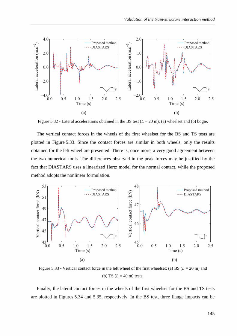
Validation of the train-structure interaction method
145
(a) (b)
Figure 5.32 - Lateral accelerations obtained in the BS test (L = 20 m): (a) wheelset and (b) bogie.
The vertical contact forces in the wheels of the first wheelset for the BS and TS tests are
plotted in Figure 5.33. Since the contact forces are similar in both wheels, only the results
obtained for the left wheel are presented. There is, once more, a very good agreement between
the two numerical tools. The differences observed in the peak forces may be justified by the
fact that DIASTARS uses a linearized Hertz model for the normal contact, while the proposed
method adopts the nonlinear formulation.
(a) (b)
Figure 5.33 - Vertical contact force in the left wheel of the first wheelset: (a) BS (L = 20 m) and
(b) TS (L = 40 m) tests.
Finally, the lateral contact forces in the wheels of the first wheelset for the BS and TS tests
are plotted in Figures 5.34 and 5.35, respectively. In the BS test, three flange impacts can be
0.0 0.5 1.0 1.5 2.0 2.5−4.0
−2.0
0.0
2.0
4.0
Time (s)
Lateral acceleration (m.s−2) Proposed method
DIASTARS
y
0.0 0.5 1.0 1.5 2.0 2.5−2.0
−1.0
0.0
1.0
2.0
Time (s)
Lateral acceleration (m.s−2) Proposed method
DIASTARS
y
0.0 0.5 1.0 1.5 2.0 2.543
45
47
49
51
53
Time (s)
Ver
tica
l co
nta
ct f
orc
e (k
N) Proposed method
DIASTARS
z
0.0 0.5 1.0 1.5 2.0 2.545
46
47
48
Time (s)
Ver
tica
l co
nta
ct f
orc
e (k
N) Proposed method
DIASTARS
z
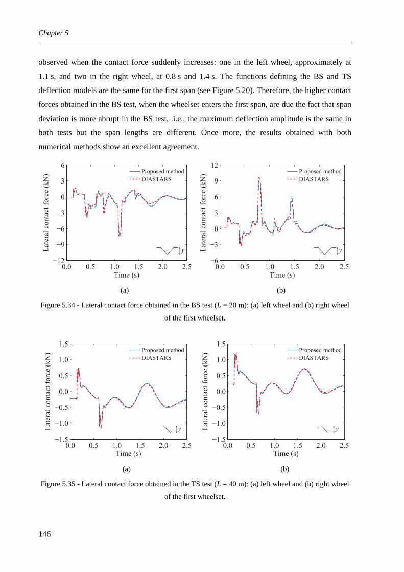
Chapter 5
146
observed when the contact force suddenly increases: one in the left wheel, approximately at
1.1 s, and two in the right wheel, at 0.8 s and 1.4 s. The functions defining the BS and TS
deflection models are the same for the first span (see Figure 5.20). Therefore, the higher contact
forces obtained in the BS test, when the wheelset enters the first span, are due the fact that span
deviation is more abrupt in the BS test, .i.e., the maximum deflection amplitude is the same in
both tests but the span lengths are different. Once more, the results obtained with both
numerical methods show an excellent agreement.
(a) (b)
Figure 5.34 - Lateral contact force obtained in the BS test (L = 20 m): (a) left wheel and (b) right wheel
of the first wheelset.
(a) (b)
Figure 5.35 - Lateral contact force obtained in the TS test (L = 40 m): (a) left wheel and (b) right wheel
of the first wheelset.
0.0 0.5 1.0 1.5 2.0 2.5−12
−9
−6
−3
0
3
6
Time (s)
Lateral contact force (kN)
DIASTARS
Proposed method
y
0.0 0.5 1.0 1.5 2.0 2.5−6
−3
0
3
6
9
12
Time (s)
Lateral contact force (kN)
DIASTARS
Proposed method
y
0.0 0.5 1.0 1.5 2.0 2.5−1.5
−1.0
−0.5
0.0
0.5
1.0
1.5
Time (s)
Lateral contact force (kN)
DIASTARS
Proposed method
y
0.0 0.5 1.0 1.5 2.0 2.5−1.5
−1.0
−0.5
0.0
0.5
1.0
1.5
Time (s)
Lateral contact force (kN)
DIASTARS
Proposed method
y

Validation of the train-structure interaction method
147
5.6 CONCLUDING REMARKS
The train-structure interaction method developed in the present thesis is validated with three
numerical applications and one experimental test.
The first application consists of reproducing four test cases based on examples presented in
Kalker (1990), in which the longitudinal and lateral creep forces are computed for distinct
ranges of creepages and semi-axes ratios of the contact ellipse. This application aims to
validate the implemented creep force models used to compute the tangential forces that appear
in the contact interface due to the rolling friction contact between wheel and rail. All the three
methods implemented in the present work proved to be adequate to deal with scenarios with
small creepages. However, the Kalker's linear model cannot predict reasonable values of the
creep forces when the creepages increase and the tangential stresses approach the saturation
limit. For higher values of translational creepages and low values of spin, both the Polach
method and the Kalker's book of tables provide adequate results, but only the latter is
sufficiently accurate for situations where the spin creepage is also higher. For these reasons, the
implemented book of tables is used in the majority of the dynamic simulations presented in this
thesis.
In the second application, the Manchester Benchmark proposed by Shackleton and Iwnicki
(2006) is revisited. The benchmark comprised a series of tests simulated with ten different
softwares with the aim of allowing an informed choice when selecting a contact model for a
particular railway vehicle simulation scenario. The tests consisted of prescribing, both statically
and dynamically, lateral displacements and yaw rotations to a single wheelset in order to
analyze its behavior. Several contact characteristics were analyzed during the benchmark,
namely the contact point positions on both wheels of the wheelset, the rolling radius difference
between wheels, the contact angles and the creepages. Generally, the results obtained with the
proposed method for all the analyzed quantities show an excellent agreement with those
obtained with widely used softwares in railway vehicle dynamics, such as GENSYS, NUCARS
and VAMPIRE. The few discrepancies observed are mainly justified by limitations of the
contact models adopted by some of the tested softwares, especially CONPOL and VOCOLIN,
rather than by limitations of the proposed method.
The third numerical example consists of evaluating the lateral stability of a single wheelset
running at several speeds. The dynamic response of the wheelset calculated with the proposed

Chapter 5
148
method is compared with that obtained using a semi-analytical model with two degrees of
freedom available in the literature (Knothe and Böhm, 1999; Valtorta et al., 2001; Wickens,
2003). The model follows a number of simplifying assumptions whereby the dynamics of the
wheelset can be described by simple linear differential equations. A good agreement between
the responses obtained with the proposed method and those obtained by the integration of the
equations of motion of the semi-analytical model is observed. As expected, for speeds below
the critical limit, both the lateral displacement and the yaw rotation of the wheelset tend to
damp out after being driven away by a lateral disturbance. This is due to the energy dissipation
provided by the creep forces and to the stability provided by the suspensions. However, when
the speed exceeds the critical value, the behavior of the wheelset becomes unstable, leading to a
hunting motion that grows indefinitely. The critical speed predicted by the proposed
formulation using a logarithmic decrement factor is also in a good agreement with the
theoretical value determined from a stability study described in Antolín (2013).
Finally, an experimental test conducted in the rolling stock test plant of the RTRI, in which a
full scale railway vehicle runs over a track that is subjected to vertical and lateral deviations, is
reproduced numerically. The lateral accelerations inside the carbody measured during the test
are compared with those obtained with the proposed method and with the train-structure
interaction software DIASTARS. The results show a good agreement, especially when the two
numerical methods are compared. Regarding the experimental results, the discrepancies
observed may be caused by the fact that vehicle is modeled using rigid bars and thus important
deformations are not considered. Furthermore, the incapacity of the actuators to reproduce with
precision the track rotations may also contribute for the differences between the experimental
and numerical results.

149
Chapter 6
RUNNING SAFETY ANALYSIS OF A HIGH-SPEED TRAIN
MOVING ON A VIADUCT UNDER SEISMIC CONDITIONS
6.1 INTRODUCTION
In the present chapter, a study regarding the running safety of a high-speed train moving on
a viaduct under seismic conditions is conducted (Montenegro et al., 2015a) using the
methodology presented in Chapter 3. The main objective of the present study consists of
evaluating the influence of the seismic intensity and track irregularities on the train running
safety. First, a description of the case study is exposed in order to introduce the viaduct, the
vehicle and the external excitation sources, namely the earthquake and the track irregularities.
The viaduct is based on an existing flyover type structure of the Portuguese railway network
situated in the city of Alverca and composed by simply supported box girders, while the vehicle
consists of a Japanese Shinkansen high-speed train whose mechanical properties were known.
The numerical models of both subsystems are developed using the finite element method
software ANSYS (2010), being their dynamic properties, namely the mode shape
configurations and respective natural frequencies, presented. The seismic action is represented
in terms of ground acceleration time-histories using artificial accelerograms that are generated
from the elastic spectra described in EN 1998‑1 (2004), with PGA corresponding to moderate
events with relatively high probability of occurrence. This type of seismic actions is of the
utmost importance, since the running safety of trains might be jeopardized not only by intense
Chapter 6
150
shakings, but also by moderate earthquakes, which may not cause significant damage to the
structure. Since no significant nonlinearity is likely to be exhibited in the piers of the viaduct
for these levels of seismicity, all the analysis are performed in the elastic domain by
considering the effective stiffness of the piers due to concrete cracking. Furthermore, and
unlike the majority of the studies in this field, the time offset between the beginning of the
earthquake and the entry of the vehicle in the viaduct is taken into account by considering
different instants in which the earthquake starts to excite the viaduct. Regarding the track
irregularities, they are also based on artificial profiles generated based on analytical PSD
functions. Then, the dynamic behavior of both the viaduct and vehicle under seismic conditions
is evaluated. For the viaduct, the vertical and lateral dynamic responses in terms of
displacements and accelerations obtained with and without earthquake are studied. Moreover,
the influence of the reduction in the stiffness of the piers due to concrete cracking on the lateral
response of the viaduct is evaluated. Regarding the vehicle, in addition to analyzing the vertical
and lateral response in terms of displacements and accelerations, the contact forces between
wheel and rail are also assessed. Special attention is given to the strong lateral impacts that
occur between the wheel flange and the rail which may lead to derailment. At the end of the
section, the influence in the response of the vehicle of both the suspension stoppers and the
time offset between the beginning of the earthquake and the entry of the vehicle in the viaduct
is analyzed. Finally, the running safety analysis of the railway vehicle running over the viaduct
is assessed based on the derailment criteria described in Section 3.5 of Chapter 3. The influence
in the running safety of the seismic intensity level, vehicle running speed and track quality is
evaluated separately. Next, all the information obtained in the dynamic analyses is condensed
in the so-called running safety charts, which consist of the global envelope of each analyzed
safety criteria as function of the running speed of the vehicle and of the seismic intensity level.
At the end of the chapter, a critical analysis about the running safety criteria adopted in the
present work is carried out.
6.2 NUMERICAL MODEL OF THE VIADUCT
6.2.1 Description of the Alverca railway viaduct
The Alverca viaduct is a flyover structure belonging to the Northern Line of the Portuguese
railway network that connects Lisbon to Porto. Its construction allowed the separation of the
rail traffic flowing in both directions and was designed for a maximum speed of 200 km/h.
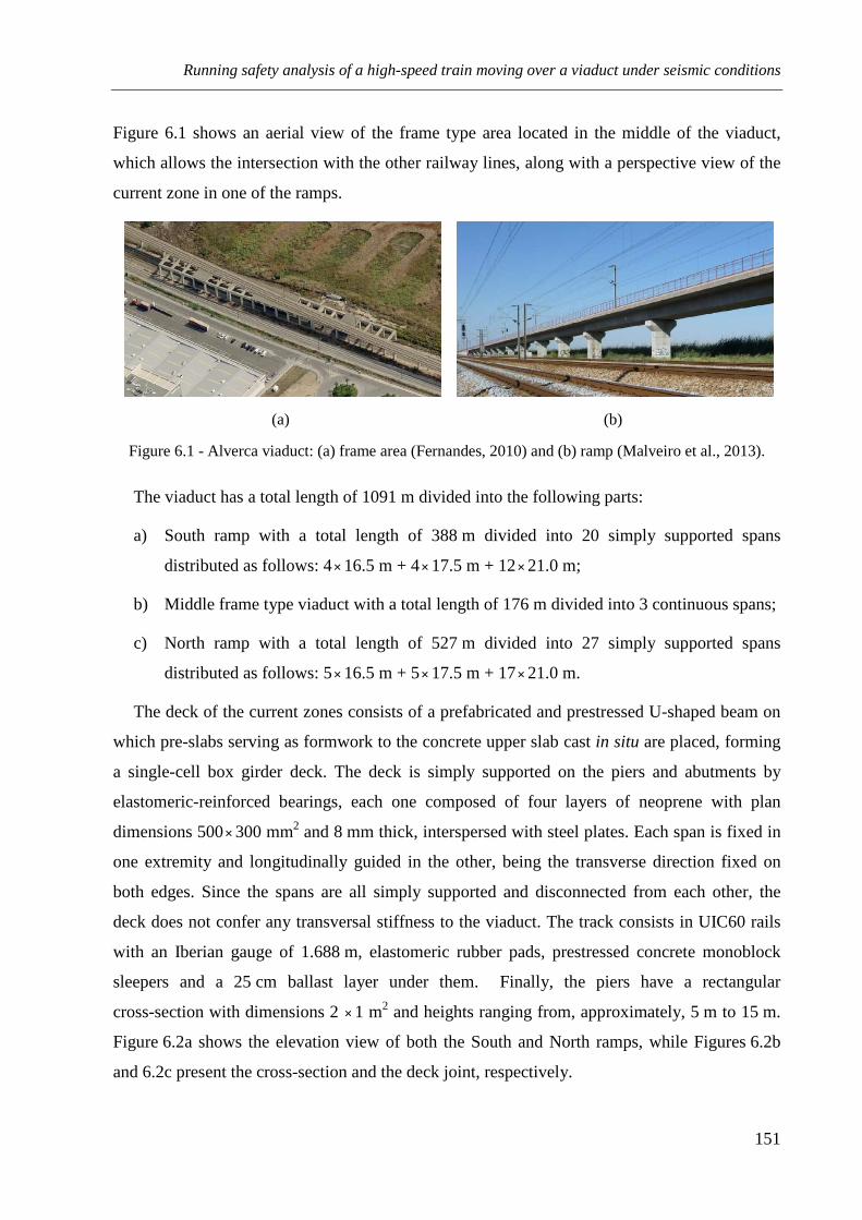
Running safety analysis of a high-speed train moving over a viaduct under seismic conditions
151
Figure 6.1 shows an aerial view of the frame type area located in the middle of the viaduct,
which allows the intersection with the other railway lines, along with a perspective view of the
current zone in one of the ramps.
(a) (b)
Figure 6.1 - Alverca viaduct: (a) frame area (Fernandes, 2010) and (b) ramp (Malveiro et al., 2013).
The viaduct has a total length of 1091 m divided into the following parts:
a) South ramp with a total length of 388 m divided into 20 simply supported spans
distributed as follows: 4× 16.5 m + 4× 17.5 m + 12× 21.0 m;
b) Middle frame type viaduct with a total length of 176 m divided into 3 continuous spans;
c) North ramp with a total length of 527 m divided into 27 simply supported spans
distributed as follows: 5× 16.5 m + 5× 17.5 m + 17× 21.0 m.
The deck of the current zones consists of a prefabricated and prestressed U-shaped beam on
which pre-slabs serving as formwork to the concrete upper slab cast in situ are placed, forming
a single-cell box girder deck. The deck is simply supported on the piers and abutments by
elastomeric-reinforced bearings, each one composed of four layers of neoprene with plan
dimensions 500× 300 mm2 and 8 mm thick, interspersed with steel plates. Each span is fixed in
one extremity and longitudinally guided in the other, being the transverse direction fixed on
both edges. Since the spans are all simply supported and disconnected from each other, the
deck does not confer any transversal stiffness to the viaduct. The track consists in UIC60 rails
with an Iberian gauge of 1.688 m, elastomeric rubber pads, prestressed concrete monoblock
sleepers and a 25 cm ballast layer under them. Finally, the piers have a rectangular
cross-section with dimensions 2 × 1 m2 and heights ranging from, approximately, 5 m to 15 m.
Figure 6.2a shows the elevation view of both the South and North ramps, while Figures 6.2b
and 6.2c present the cross-section and the deck joint, respectively.

Chapter 6
152
(a)
(b) (c)
Figure 6.2 - Blueprints of the Alverca viaduct: (a) elevation view of the South and North ramps;
(b) cross-section and (c) deck joint above the pier.
6.2.2 Finite element model of the idealized viaduct
The structure used in the present study is based on the Alverca viaduct described in the
previous section. However, for simplicity of the model, an idealized structure with a total
length of 630 m divided into 30 simply supported spans with 21 m length each and supported
by piers with 10 m height is adopted in the present study. The geometrical properties of both
the deck and the piers are the same as the original viaduct.
The numerical model of the viaduct is developed in ANSYS. The deck, piers, sleepers and
rails are modeled using beam finite elements, while the bearing supports, ballast and pads are
modeled using linear spring-dampers. Mass point elements are also used to model the ballast
mass and the non-structural elements such as safeguards and edge beams of the deck. The
connection between the top of the piers and the deck, as well as the connection between the
deck and the track, is accomplished by rigid frame elements. In order to guarantee a correct
21.0 21.0 21.0 21.0 16.5 17.517.0 21.0 21.0 21.0 21.0 16.5 17.5 21.0 21.0 21.0 16.5 17.5 21.0 21.0 16.5 17.521.0 21.0 21.0 16.521.0
16.5 21.0 21.0 21.0 17.5 16.5 21.0 21.0 21.0 17.5 16.5 21.0 21.0 21.0 17.5 16.5 21.0 21.0 21.0 17.0
North ramp
South ramp
2.00
4.30
7.20
1.20
3.00
0.180.20
0.15
0.65
prefabricated beam
ballast layer
column
pre-slabin-situ slab
0.29
0.50bearings
1.00
0.65
0.50
1.20
0.15
0.29
0.60 0.60 0.60 0.60 0.60
ballast layer
prefabricated
beam
in-situ slab
sleepers
rail
1.50
column
bearings
pre-slab

Running safety analysis of a high-speed train moving over a viaduct under seismic conditions
153
representation of the transition zones between the structure and the embankment, an extension
of the track is modeled in both extremities of the viaduct.
Special focus is given to the track modeling, since it may strongly influence the behavior of
the vehicle. This is one of the advantages of using the finite element method to model the
structure, since in the majority of studies performed in multibody platforms the track is
considered to be rigid, which is far from reality.
A schematic representation of the numerical model, along with a detail of the cross-section
and the deck joint above the piers is illustrated in Figure 6.3 (the track is not included in
Figure 6.3a for simplicity), while Figure 6.4 presents a partial overview and two details of the
numerical model of the viaduct developed in ANSYS. Although the spans are disconnected
from each other, the track mobilizes a certain amount of transversal stiffness when relative
movements between adjacent spans occur, as can be seen in the detail of the joint depicted in
Figure 6.3c.
(a)
(b) (c)
Figure 6.3 - Numerical model of the viaduct: (a) elevation view, (b) cross-section and (c) deck joint.
21 m 21 m
30 x 21 m
. . .
. . .
. . .
. . .
10
m
deck element rigid link
21 m21 m
rigid linkdeck element
pier
element
. . .
pier
element
Figure 6.3c
See detail in
supports
pier
sleeperrail
deck ballastrigid
links
fasteners
(springs)
(beam)
(beam)
(beam) (spring-dampers)
(beam)
(spring-dampers & point masses)
pier(beam)
bearing supports(springs)
deck(beam)
ballast(spring-dampers & point masses)
sleeper(beam)
fasteners(spring-dampers)
rail(beam)
rigidlinks
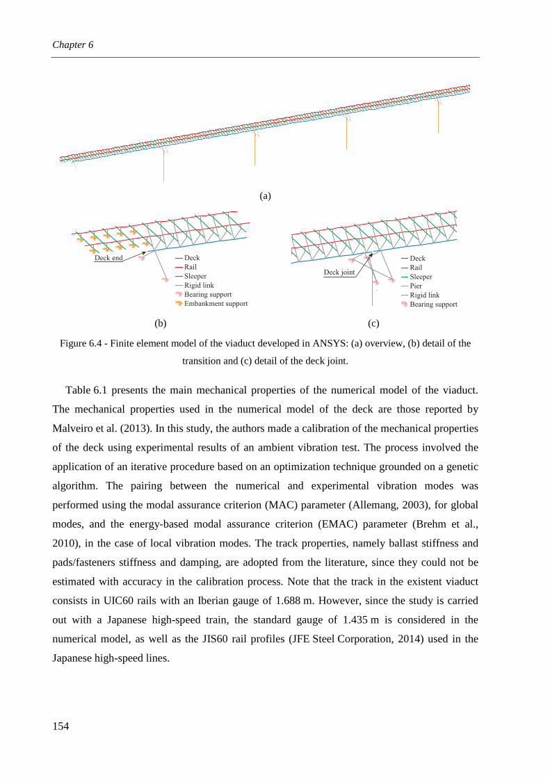
Chapter 6
154
(a)
(b) (c)
Figure 6.4 - Finite element model of the viaduct developed in ANSYS: (a) overview, (b) detail of the
transition and (c) detail of the deck joint.
Table 6.1 presents the main mechanical properties of the numerical model of the viaduct.
The mechanical properties used in the numerical model of the deck are those reported by
Malveiro et al. (2013). In this study, the authors made a calibration of the mechanical properties
of the deck using experimental results of an ambient vibration test. The process involved the
application of an iterative procedure based on an optimization technique grounded on a genetic
algorithm. The pairing between the numerical and experimental vibration modes was
performed using the modal assurance criterion (MAC) parameter (Allemang, 2003), for global
modes, and the energy-based modal assurance criterion (EMAC) parameter (Brehm et al.,
2010), in the case of local vibration modes. The track properties, namely ballast stiffness and
pads/fasteners stiffness and damping, are adopted from the literature, since they could not be
estimated with accuracy in the calibration process. Note that the track in the existent viaduct
consists in UIC60 rails with an Iberian gauge of 1.688 m. However, since the study is carried
out with a Japanese high-speed train, the standard gauge of 1.435 m is considered in the
numerical model, as well as the JIS60 rail profiles (JFE Steel Corporation, 2014) used in the
Japanese high-speed lines.
Deck
Rail
Sleeper
Rigid link
Bearing support
Embankment support
Deck end
Deck joint
Deck
Rail
Sleeper
Pier
Bearing support
Rigid link

Running safety analysis of a high-speed train moving over a viaduct under seismic conditions
155
Table 6.1 - Mechanical properties of the numerical model of the viaduct.
Parameter Designation Value Unit Reference
Ec,slab Modulus of elasticity of the concrete of the upper slab
33.48 GPa Malveiro et al. (2013)
Ec,beam Modulus of elasticity of the
concrete of the prefabricated beam 48.08 GPa Malveiro et al. (2013)
Ec,sleeper Modulus of elasticity of the
concrete of the sleeper 40.90 GPa Malveiro et al. (2013)
Ec,pier Modulus of elasticity of the
concrete of the pier 33.00 GPa EN 1992-1-1 (2004)
ρc Density of concrete 2590.4 kg/m3 Malveiro et al. (2013)
ρbal Density of ballast 1995.9 kg/m3 Malveiro et al. (2013)
Kbal,l Ballast's longitudinal stiffness 30 MN/m/m UIC 774-3-R (2001)
Kbal,t Ballast's transversal stiffness 7.5 MN/m/m ERRI D 202/RP 11 (1999)
Kbal,v Ballast's vertical stiffness 100 MN/m/m ERRI D 202/RP 11 (1999)
Cbal Ballast's damping (3 directions) 50 kN.s/m/m Wu and Yang (2003)
Kfas,l Fastener's longitudinal stiffness 20 MN/m Zhai et al. (2009)
Kfas,t Fastener's transversal stiffness 20 MN/m Zhai et al. (2009)
Kfas,v Fastener's vertical stiffness 500 MN/m ERRI D 214/RP 5 (1999)
Kfas,r Fastener's rotational stiffness 45 kN.m/rad ERRI D 202/RP 11 (1999)
Cfas,l Fastener's longitudinal damping 50 kN.s/m Zhai et al. (2009)
Cfas,t Fastener's transversal damping 50 kN.s/m Zhai et al. (2009)
Cfas,v Fastener's vertical damping 200 kN.s/m ERRI D 214/RP 5 (1999)
Kl Longitudinal stiffness of the
bearing supports 4.4 MN/m Malveiro et al. (2013)
Kv Vertical stiffness of the bearing
supports 5200 MN/m Malveiro et al. (2013)
6.2.3 Dynamic properties of the viaduct
The first mode shapes and natural frequencies of the viaduct are plotted in Figure 6.5. Since
all the spans are simply supported and disconnected from each other (see Figure 6.3c), the
frequencies of the first modes are identical, i.e., the global frequencies of the viaduct are mainly
controlled by the first mode of the piers. The small differences observed are due to the fact that
the track confers a slight amount of stiffness to the deck in the transversal direction.
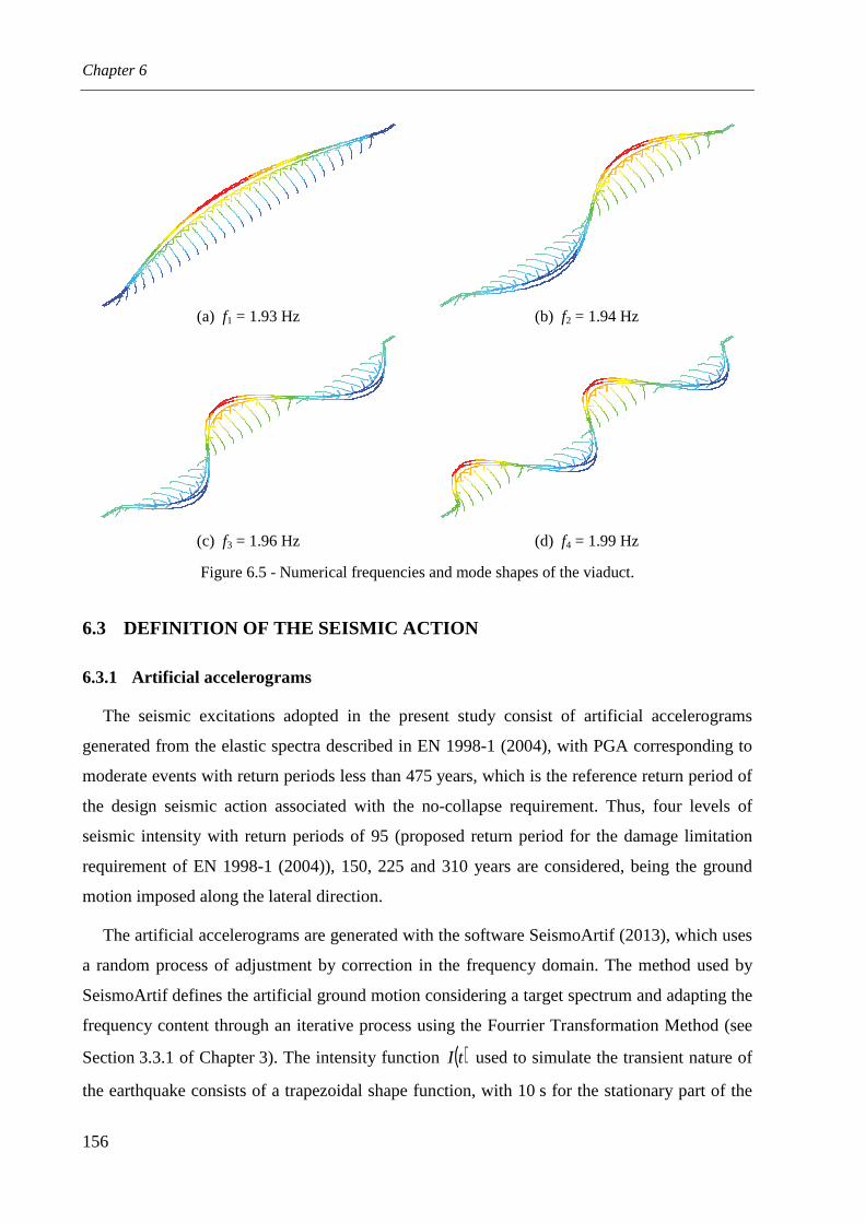
Chapter 6
156
(a) f1 = 1.93 Hz (b) f2 = 1.94 Hz
(c) f3 = 1.96 Hz (d) f4 = 1.99 Hz
Figure 6.5 - Numerical frequencies and mode shapes of the viaduct.
6.3 DEFINITION OF THE SEISMIC ACTION
6.3.1 Artificial accelerograms
The seismic excitations adopted in the present study consist of artificial accelerograms
generated from the elastic spectra described in EN 1998-1 (2004), with PGA corresponding to
moderate events with return periods less than 475 years, which is the reference return period of
the design seismic action associated with the no-collapse requirement. Thus, four levels of
seismic intensity with return periods of 95 (proposed return period for the damage limitation
requirement of EN 1998-1 (2004)), 150, 225 and 310 years are considered, being the ground
motion imposed along the lateral direction.
The artificial accelerograms are generated with the software SeismoArtif (2013), which uses
a random process of adjustment by correction in the frequency domain. The method used by
SeismoArtif defines the artificial ground motion considering a target spectrum and adapting the
frequency content through an iterative process using the Fourrier Transformation Method (see
Section 3.3.1 of Chapter 3). The intensity function ( )tI used to simulate the transient nature of
the earthquake consists of a trapezoidal shape function, with 10 s for the stationary part of the

Running safety analysis of a high-speed train moving over a viaduct under seismic conditions
157
accelerogram (minimum value according to EN 1998-1 (2004)) and 2 s of slope in each
extremity, as shown in Figure 6.6.
Figure 6.6 - Intensity function adopted in the present study.
The target elastic spectra are defined for the seismic zone 2.3 of the Portuguese territory and
for a soil type A (EN 1998-1-NA, 2009), with an importance factor of 1.0, as proposed by EN
1998-2 (2005) for railway bridges, and a viscous damping of 5 %. The PGA corresponding to
the return periods T of the seismic actions considered in this work are presented in Table 6.2.
Table 6.2 - PGA corresponding to the return periods of the seismic actions1.
T (years) 95 150 225 310
PGA (m.s-2) 0.862 1.050 1.250 1.420
The artificial ground motions generated with SeismoArtif and the respective response
spectrum adjustments to the target spectrum are plotted in Figures 6.7 to 6.10.
(a) (b)
Figure 6.7 - Generated ground motion for T = 95 years: (a) accelerogram and (b) spectrum adjustment.
1 The values of the PGA were kindly provided by the National Laboratory for Civil Engineering of Portugal.
−1.0
−0.5
0.0
0.5
1.0
Time (s)
Inte
nsi
ty I
(t)
0 2 4 6 8 10 12 14
I(t)
0 2 4 6 8 10 12 14−1.5
−1.0
−0.5
0.0
0.5
1.0
1.5
Time (s)
Ground acceleration (m.s−2)
0 1 2 3 40.0
1.0
2.0
3.0
4.0
Period (s)
Spec
tral
acc
eler
atio
n (
m.s
−2) Target spectrum EC8
Target spectrum EC8 + 10%Target spectrum EC8 − 10%Generated spectrum
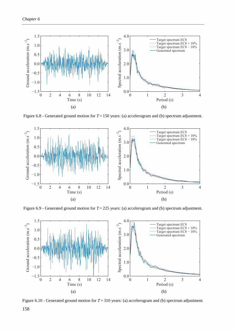
Chapter 6
158
(a) (b)
Figure 6.8 - Generated ground motion for T = 150 years: (a) accelerogram and (b) spectrum adjustment.
(a) (b)
Figure 6.9 - Generated ground motion for T = 225 years: (a) accelerogram and (b) spectrum adjustment.
(a) (b)
Figure 6.10 - Generated ground motion for T = 310 years: (a) accelerogram and (b) spectrum adjustment.
0 2 4 6 8 10 12 14−1.5
−1.0
−0.5
0.0
0.5
1.0
1.5
Time (s)
Ground acceleration (m.s−2)
0 1 2 3 40.0
1.0
2.0
3.0
4.0
Period (s)
Spec
tral
acc
eler
atio
n (
m.s
−2) Target spectrum EC8
Target spectrum EC8 + 10%Target spectrum EC8 − 10%Generated spectrum
0 2 4 6 8 10 12 14−1.5
−1.0
−0.5
0.0
0.5
1.0
1.5
Time (s)
Ground acceleration (m.s−2)
0 1 2 3 40.0
1.0
2.0
3.0
4.0
Period (s)
Sp
ectr
al a
ccel
erat
ion
(m
.s−
2) Target spectrum EC8
Target spectrum EC8 + 10%Target spectrum EC8 − 10%Generated spectrum
0 2 4 6 8 10 12 14−1.5
−1.0
−0.5
0.0
0.5
1.0
1.5
Time (s)
Ground acceleration (m.s−2)
0 1 2 3 40.0
1.0
2.0
3.0
4.0
Period (s)
Spec
tral
acc
eler
atio
n (
m.s
−2) Target spectrum EC8
Target spectrum EC8 + 10%Target spectrum EC8 − 10%Generated spectrum

Running safety analysis of a high-speed train moving over a viaduct under seismic conditions
159
6.3.2 Time offset between the beginning of the earthquake and the entry of the vehicle in
the viaduct
The random nature of the seismic events makes it impossible to predict the position of the
vehicle in the moment the earthquake starts. Therefore, and unlike the majority of studies in
this field, in which the earthquake is assumed to start at the instant the train enters the bridge,
the time offset between the beginning of the earthquake and the entry of the vehicle in the
viaduct is taken into account by considering five scenarios corresponding to different instants
in which the earthquake starts to excite the viaduct. This procedure to cover covering a wider
range of combinations for a more extensive study.
The coordinate of the first wheelset xi at the instant the earthquake starts is presented in
Figure 6.11. The coordinate xi is defined with respect to the coordinate system (x, y) positioned
at the beginning of the viaduct and the subscripts ni ...,,2,1= indicate the scenario number.
Figure 6.11 - Coordinate of the first wheelset at the instant the earthquake starts.
The first scenario represents the case in which the vehicle enters the viaduct in the instant
the earthquake stops, while the last scenario represents a situation in which the earthquake
starts in the instant the vehicle leaves the viaduct. The other scenarios will cover the
intermediate situations. Hence, for each scenario i, the coordinate of the first wheelset ix at the
instant the earthquake starts is given by
( )
−+−+−=
11
n
ttitVx ve
ei (6.1)
where V is the vehicle speed, et is the earthquake duration and vt is the time that the vehicle
takes to cross the viaduct. Note that the coordinate ix is negative in the scenarios in which the
vehicle enters the viaduct after the beginning of the earthquake. This is to ensure that, for these
scenarios, the simulations initiate with the beginning of the ground motion. On the other hand,
in the scenarios in which the earthquake starts when the vehicle is already on the viaduct, the
. . .
Viaduct edge
Viaduct length
V
y
x
xi
V.t
gaɺɺ

Chapter 6
160
simulation begins with the vehicle positioned at its edge. This procedure aims to guarantee that
the vehicle is already excited due to the track irregularities and due to the interaction with the
structure at the instant the earthquake starts. Figure 6.12 schematizes the position of the vehicle
at the start of the simulation for the two aforementioned types of scenarios.
(a)
(b)
Figure 6.12 - Position of the vehicle at the start of the simulation: (a) the vehicle enters the viaduct after
the beginning of the earthquake and (b) before the beginning of the earthquake.
6.4 MODELING OF THE SEISMIC BEHAVIOR OF THE PIERS
The seismic actions considered in the present study correspond to moderate events with
relatively high probability of occurrence, as shown in Section 6.3.1. Although no significant
damage to the structure is expected for these levels of intensity, the reduction in the piers'
stiffness due to concrete cracking should be accounted. Thus, the effective stiffness of the piers
is evaluated based on the methodology described in Section 3.4 of the Chapter 3.
6.4.1 Monotonic response of the piers
The first step of the methodology consists of performing a nonlinear monotonic static
analysis to evaluate the horizontal response of the piers. In this analysis, the idealized
representation of the structure is subjected to a constant gravity load and to a monotonically
increasing displacement that represent the inertial effects from the earthquake. Since the force
is increased until the ultimate capacity of the pier is reached, the model has to account for the
effects of both the material inelasticity and the geometric nonlinearity.
. .
Viaduct edge
Viaduct length
V
y
x
V.t
gaɺɺ.
. .
Viaduct edge
Viaduct length
V
y
x
V.t
gaɺɺ.
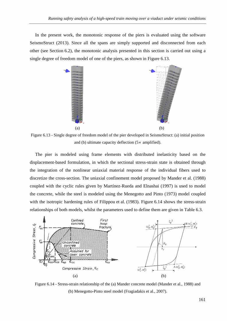
Running safety analysis of a high-speed train moving over a viaduct under seismic conditions
161
In the present work, the monotonic response of the piers is evaluated using the software
SeismoStruct (2013). Since all the spans are simply supported and disconnected from each
other (see Section 6.2), the monotonic analysis presented in this section is carried out using a
single degree of freedom model of one of the piers, as shown in Figure 6.13.
(a) (b)
Figure 6.13 - Single degree of freedom model of the pier developed in SeismoStruct: (a) initial position
and (b) ultimate capacity deflection (5× amplified).
The pier is modeled using frame elements with distributed inelasticity based on the
displacement-based formulation, in which the sectional stress-strain state is obtained through
the integration of the nonlinear uniaxial material response of the individual fibers used to
discretize the cross-section. The uniaxial confinement model proposed by Mander et al. (1988)
coupled with the cyclic rules given by Martínez-Rueda and Elnashai (1997) is used to model
the concrete, while the steel is modeled using the Menegotto and Pinto (1973) model coupled
with the isotropic hardening rules of Filippou et al. (1983). Figure 6.14 shows the stress-strain
relationships of both models, whilst the parameters used to define them are given in Table 6.3.
(a) (b)
Figure 6.14 - Stress-strain relationship of the (a) Mander concrete model (Mander et al., 1988) and
(b) Menegotto-Pinto steel model (Fragiadakis et al., 2007).

Chapter 6
162
Table 6.3 - Parameters of the nonlinear constitutive material models.
Concrete C30/37 Steel S500
Parameter Value Parameter Value
Compressive strength 38 MPa Modulus of elasticity 200 GPa
Tensile strength 2.9 MPa Yield strength 500 MPa
Strain at peak stress 0.002 Strain hardening parameter 0.005
Specific weight 24 kN/m3 Specific weight 78 kN/m3
The piers are designed according to the specifications proposed in the EN 1998-2 (2005) for
the seismic zones 1.4 and 2.3 of the Portuguese territory, soil type A (EN 1998-1-NA, 2009)
and using a behavior factor of 2.5. The dimensions of the existing cross-sections from the
Alverca viaduct (see Section 6.2.1) were adopted, leading to a reinforcement ratio of 0.41 %.
Figure 6.15 presents the force-displacement capacity curve of the piers obtained in the
monotonic analysis. The piers begin to crack for a base shear force Fb,cr of approximately
298 kN and fail for displacements of 0.5 m. The figure also shows the location of the yield
region of the pier. The perturbations in the curve are the result of difficulties in reproducing the
tensile behavior of the concrete when cracking occurs.
Figure 6.15 - Capacity curve of the piers.
6.4.2 Nonlinear dynamic analysis
The second step for the estimation of the effective stiffness consists of performing a
nonlinear dynamic analysis to predict the inelastic response of the piers subjected to the seismic
ground motions described in Section 6.3. The finite element model used in this analysis is the
same as that presented in the previous section, but with a lumped mass of 281 t positioned
above the top of the pier at the center of gravity of the deck cross-section, representing the mass
0.0 0.1 0.2 0.3 0.4 0.50
200
400
600
800
Displacement (m)
Bas
e sh
ear
(kN
)
, 298kNb crF ≃
Yield region

Running safety analysis of a high-speed train moving over a viaduct under seismic conditions
163
of the deck. Again, the software SeismoStruct is used to perform the nonlinear dynamic
analysis.
The energy dissipation mechanism is accounted by means of Rayleigh damping (Clough and
Penzien, 2003), with an equivalent viscous damping ratio of 2 % fixed in fela = 1.84 Hz,
corresponding to the frequency obtained with an uncracked cross-section, and in feff = 0.76 Hz,
which corresponds to the frequency of the pier with an effective stiffness estimated with the
procedure described in the Annex C of EN 1998-2 (2005) for reinforced concrete ductile
members. This criterion is based on the fact that the natural frequency of the piers after the
calibration of the effective flexural stiffness is somewhere between the two aforementioned
frequencies. The Rayleigh damping curve adopted in the present analysis, and also in the
train-structure interaction dynamic analyses described later, is plotted in Figure 6.16.
Figure 6.16 - Relation between damping ratio and frequency according to the Rayleigh damping.
The time-history responses at the top of the pier, as well as the base shear force obtained for
the seismic load cases with return periods T of 95 and 310 years, are shown in Figure 6.17 for
exemplification purposes, being the remaining results summarized in Table 6.4. It can be
observed that the piers do not exhibit significant nonlinearity, since the maximum
displacements δmax obtained for all the seismic cases adopted in this work are still far from
reaching the yield region (see Figure 6.15 and Table 6.4). This behavior was expected, since
the piers are designed for a seismic action associated with the no-collapse requirement defined
by the EN 1998-1 (2004) (T = 475 years). However, the maximum base shear Fb,max exceeds
Fb,cr in all the analyses, making it necessary to use a lower stiffness for the piers in the
train-structure dynamic analyses performed in the elastic domain.
0 1 2 3 4 50
1
2
3
4
Frequency (Hz)
Dam
pin
g r
atio
(%
)
Combined dampingStiffness proporcionalMass proporcional
0.7
6H
zef
ff
=
1.8
4H
zel
af
=
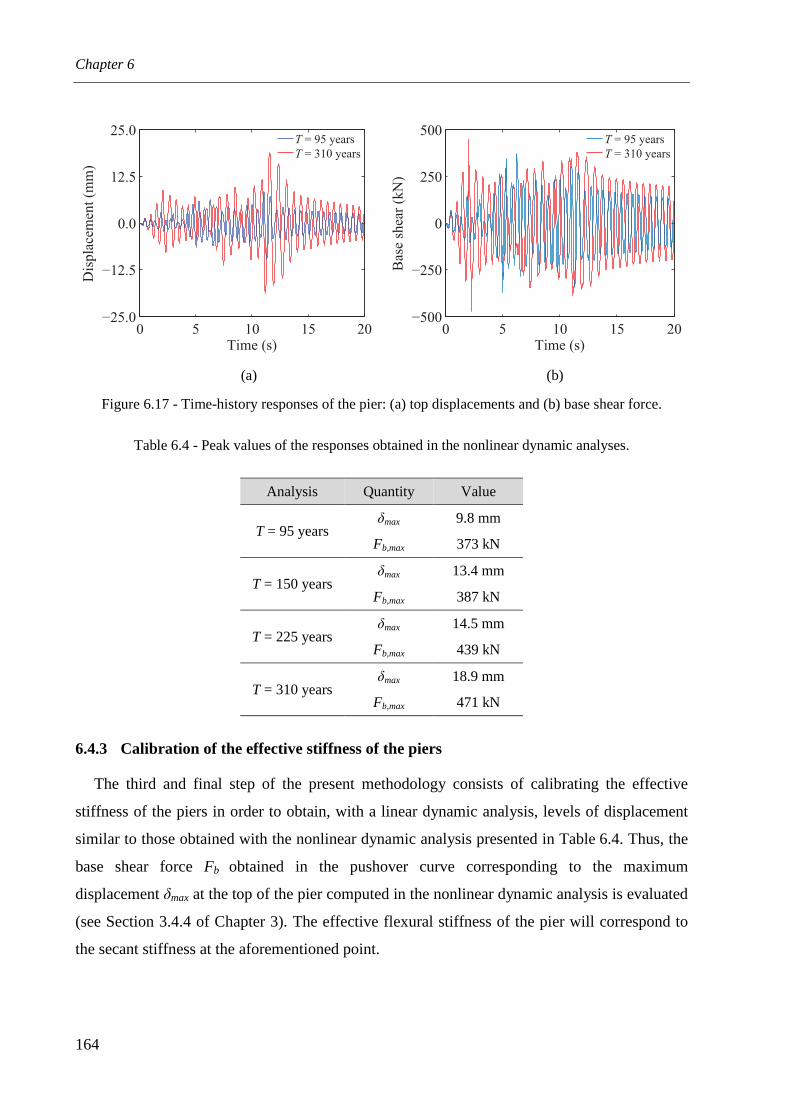
Chapter 6
164
(a) (b)
Figure 6.17 - Time-history responses of the pier: (a) top displacements and (b) base shear force.
Table 6.4 - Peak values of the responses obtained in the nonlinear dynamic analyses.
Analysis Quantity Value
T = 95 years δmax 9.8 mm
Fb,max 373 kN
T = 150 years δmax 13.4 mm
Fb,max 387 kN
T = 225 years δmax 14.5 mm
Fb,max 439 kN
T = 310 years δmax 18.9 mm
Fb,max 471 kN
6.4.3 Calibration of the effective stiffness of the piers
The third and final step of the present methodology consists of calibrating the effective
stiffness of the piers in order to obtain, with a linear dynamic analysis, levels of displacement
similar to those obtained with the nonlinear dynamic analysis presented in Table 6.4. Thus, the
base shear force Fb obtained in the pushover curve corresponding to the maximum
displacement δmax at the top of the pier computed in the nonlinear dynamic analysis is evaluated
(see Section 3.4.4 of Chapter 3). The effective flexural stiffness of the pier will correspond to
the secant stiffness at the aforementioned point.
0 5 10 15 20−25.0
−12.5
0.0
12.5
25.0
Time (s)
Displacement (mm)
T = 95 years
T = 310 years
0 5 10 15 20−500
−250
0
250
500
Time (s)
Base shear (kN)
T = 95 years
T = 310 years

Running safety analysis of a high-speed train moving over a viaduct under seismic conditions
165
In the present study, since all spans of the viaduct are simply supported and disconnected
from each other, the stiffness of the deck does not significantly influence the lateral behavior of
the viaduct. Therefore, the effective flexural stiffness of the pier EIeff can be calculated based
on the elastic deflection of a cantilever beam subjected to a concentrated load, given by
( )xhEI
xF
eff
bmax −= 3
6
2
δ (6.2)
where h is the total height of the cantilever, from the base of the pier to the center of gravity of
the deck, and x is the position in which the displacement is being computed, which in this case
corresponds to the top of the pier.
In order to avoid the dependency of the model on the intensity of the action, the minimum
effective flexural stiffness obtained with the strongest excitation is adopted in all calculations.
Nevertheless, although the analyses with lower seismic intensities are performed with a more
flexible model, the aforementioned assumption ensures an acceptable approximation of the
stiffness of the piers, especially in the most critical scenarios when the viaduct is subjected to
stronger excitations. Hence, the proposed methodology leads to a value of the effective flexural
stiffness EIeff of about 43 % the value of the elastic flexural stiffness EI0.
The comparison between the responses of the piers subjected to the seismic action with
T = 310 years, in terms of displacements at the top and shear force at the base, obtained with
the nonlinear dynamic analysis described in Section 6.4.2 and with a linear dynamic analysis
with effective stiffness, is presented in Figure 6.18. A good agreement can be observed
between the linear and nonlinear results in terms of maximum displacements and shear forces.
Regarding the global response, the differences were expected, being justified by the fact that, at
the beginning of the analysis, the nonlinear model is still with the elastic stiffness, while the
linear model is already with a stiffness corresponding to the cracked section. However, when
the nonlinear model begins to crack, the responses obtained with both models become similar
in terms of maximum values.

Chapter 6
166
(a) (b)
Figure 6.18 - Time-history responses of the pier for the seismic action with T = 310 years: (a) top
displacements and (b) base shear force.
6.4.4 Dynamic properties of the viaduct considering the effective stiffness of the piers
The mode shapes and natural frequencies of the viaduct considering the effective stiffness of
the piers are plotted in Figure 6.19. As expected, the modes are identical to those presented in
Figure 6.5, but with lower frequencies due to the reduced stiffness of the piers.
.
(a) f1 = 1.27 Hz (b) f2 = 1.28 Hz
(c) f3 = 1.31 Hz (d) f4 = 1.34 Hz
Figure 6.19 - Numerical frequencies and mode shapes of the viaduct after calibration of the effective
stiffness of the piers.
0 5 10 15 20−25.0
−12.5
0.0
12.5
25.0
Time (s)
Displacement (mm)
Nonlinear
Linear EIeff
0 5 10 15 20−500
−250
0
250
500
Time (s)
Base shear (kN)
Nonlinear
Linear EIeff

Running safety analysis of a high-speed train moving over a viaduct under seismic conditions
167
6.5 NUMERICAL MODEL OF THE VEHICLE
6.5.1 Description of the Shinkansen high-speed train
The vehicle used in the present work for the dynamic analysis is based on a Japanese
Shinkansen high-speed train (see Figure 6.20). This train was chosen for carrying out the
running safety study since its geometrical and mechanical properties were provided by the
RTRI2.
Figure 6.20 - Examples of Shinkansen trains used in Japan (Wikipedia/Shinkansen, 2014).
The train is a conventional type train with all the eight cars independent from each other
with 25 m length each. Since the traction is distributed along the whole train, the cars are
identical in terms of geometrical and mechanical properties, being the total weight of each car
45 t. Figure 6.21 illustrates the load model of the adopted train, including the static axle load of
110 kN of each wheelset and the longitudinal distances between them.
Figure 6.21 - Load model of the Shinkansen high-speed train.
6.5.2 Finite element model of the vehicle
As with the structure, the numerical model of the vehicle is also developed in ANSYS. A
schematic representation of the dynamic model of one of the cars is illustrated in Figure 6.22.
2 The geometrical and mechanical properties of the Shinkansen train are not published due to confidential matters from the manufacturer.
2.50 15.00
. . .
car 8
. . .
. . .
6 x car
11
0 k
N
11
0 k
N
11
0 k
N
11
0 k
N
11
0 k
N
11
0 k
N
2.50 2.50 2.50 2.50 2.50
. . .
11
0 k
N
11
0 k
N
11
0 k
N
11
0 k
N
11
0 k
N
11
0 k
N
2.50 2.50 2.50 2.50 2.50 2.50
car 1
15.00

Chapter 6
168
The springs and dampers of the suspensions are denoted by k and c and the masses and rotary
inertias are indicated by m and I. The longitudinal, lateral and vertical distances are denoted by
a, b and h, respectively, Lcp refers to the lateral distance between the initial contact points and
R0 is the nominal rolling radius. The subscripts cb, bg and ws indicate carbody, bogie and
wheelset, respectively.
(a) (b)
Figure 6.22 - Dynamic model of the railway vehicle: (a) lateral view and (b) front view.
The carbody, bogies and wheelsets are modeled using beam finite elements, while the
suspensions are modeled using spring-dampers in the three directions, as shown in Figure 6.23.
The springs used to model the suspensions are characterized by bilinear laws, as shown in
Figure 6.22b, except the one used to model the secondary transversal suspension. This
suspension follows a multilinear law to simulate the presence of rubber stoppers whose
stiffness increases gradually (Matsumoto et al., 2004). These stoppers are used to avoid large
lateral displacements of the carbody, especially during earthquake. Finally, the masses and
rotary inertias are modeled using mass point elements, located at the center of mass of each
component (see Figure 6.23). The wheel profile adopted in the contact model is the same as
that used in the validation application presented in Section 5.5 of Chapter 5.
No material damping is considered in the model, since the flexibility of the several
components of the car, such as the carbody, bogies and wheelsets, is not accounted in the beam
elements used for modeling them.
,cb cbm I
2, 2,,z zk c
1a /2
2, 2,,z zk c
2a
1, 1,,z zk c1, 1,,z zk c
1a /2
,bg bgm I ,bg bgm I
,ws wsm I
F
δ
bilinear
δ
F
multilinear
1, 1,,y yk c
1, 1,,x xk c1, 1,,z zk c
2, 2,,z zk c
2, 2,,y yk c2, 2,,x xk c
1h
2h
3h
0R
1b
2b
3b
,cb cbm I
2Lcp
,bg bgm I
,ws wsm I
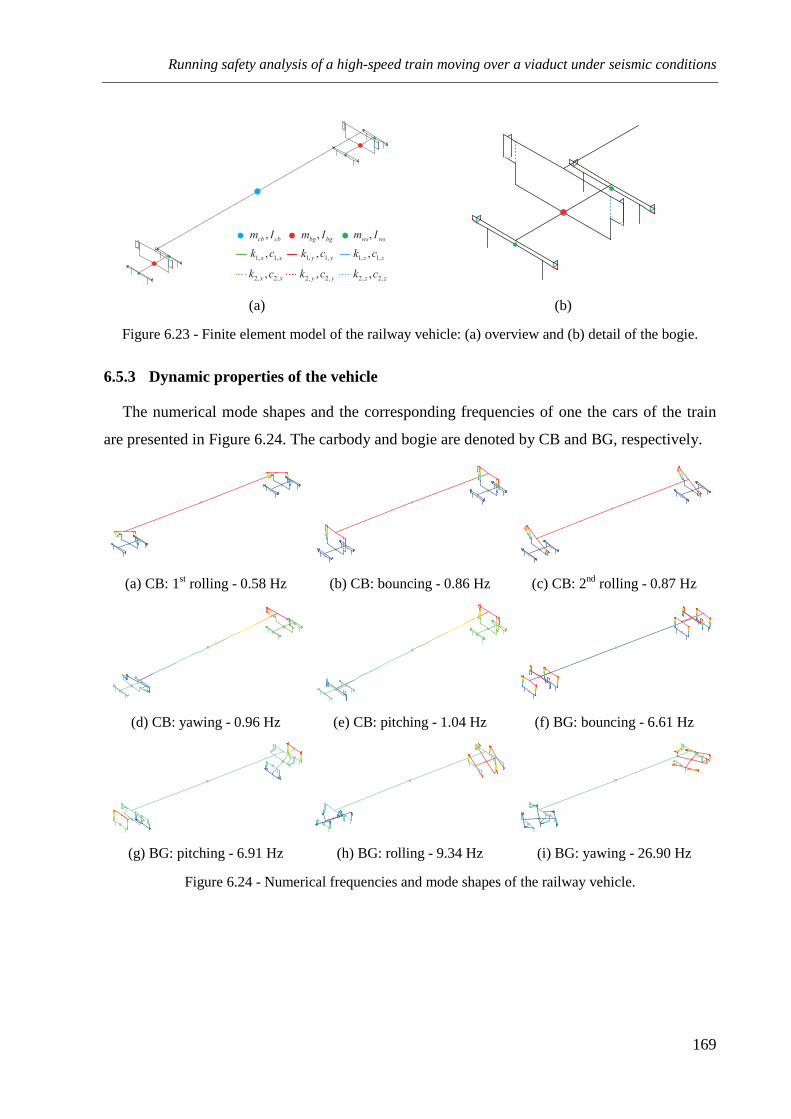
Running safety analysis of a high-speed train moving over a viaduct under seismic conditions
169
(a) (b)
Figure 6.23 - Finite element model of the railway vehicle: (a) overview and (b) detail of the bogie.
6.5.3 Dynamic properties of the vehicle
The numerical mode shapes and the corresponding frequencies of one the cars of the train
are presented in Figure 6.24. The carbody and bogie are denoted by CB and BG, respectively.
(a) CB: 1st rolling - 0.58 Hz (b) CB: bouncing - 0.86 Hz (c) CB: 2nd rolling - 0.87 Hz
(d) CB: yawing - 0.96 Hz (e) CB: pitching - 1.04 Hz (f) BG: bouncing - 6.61 Hz
(g) BG: pitching - 6.91 Hz (h) BG: rolling - 9.34 Hz (i) BG: yawing - 26.90 Hz
Figure 6.24 - Numerical frequencies and mode shapes of the railway vehicle.
,cb cbm I
1, 1,,x xk c
1, 1,,y yk c 1, 1,,z zk c
2, 2,,z zk c2, 2,,y yk c2, 2,,x xk c
,bg bgm I ,ws wsm I
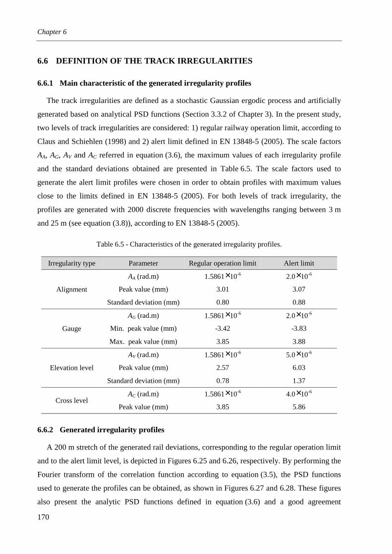
Chapter 6
170
6.6 DEFINITION OF THE TRACK IRREGULARITIES
6.6.1 Main characteristic of the generated irregularity profiles
The track irregularities are defined as a stochastic Gaussian ergodic process and artificially
generated based on analytical PSD functions (Section 3.3.2 of Chapter 3). In the present study,
two levels of track irregularities are considered: 1) regular railway operation limit, according to
Claus and Schiehlen (1998) and 2) alert limit defined in EN 13848-5 (2005). The scale factors
AA, AG, AV and AC referred in equation (3.6), the maximum values of each irregularity profile
and the standard deviations obtained are presented in Table 6.5. The scale factors used to
generate the alert limit profiles were chosen in order to obtain profiles with maximum values
close to the limits defined in EN 13848-5 (2005). For both levels of track irregularity, the
profiles are generated with 2000 discrete frequencies with wavelengths ranging between 3 m
and 25 m (see equation (3.8)), according to EN 13848-5 (2005).
Table 6.5 - Characteristics of the generated irregularity profiles.
Irregularity type Parameter Regular operation limit Alert limit
Alignment
AA (rad.m) 1.5861×10⁻⁶ 2.0×10⁻⁶
Peak value (mm) 3.01 3.07
Standard deviation (mm) 0.80 0.88
Gauge
AG (rad.m) 1.5861×10⁻⁶ 2.0×10⁻⁶
Min. peak value (mm) -3.42 -3.83
Max. peak value (mm) 3.85 3.88
Elevation level
AV (rad.m) 1.5861×10⁻⁶ 5.0×10⁻⁶
Peak value (mm) 2.57 6.03
Standard deviation (mm) 0.78 1.37
Cross level AC (rad.m) 1.5861×10⁻⁶ 4.0×10⁻⁶
Peak value (mm) 3.85 5.86
6.6.2 Generated irregularity profiles
A 200 m stretch of the generated rail deviations, corresponding to the regular operation limit
and to the alert limit level, is depicted in Figures 6.25 and 6.26, respectively. By performing the
Fourier transform of the correlation function according to equation (3.5), the PSD functions
used to generate the profiles can be obtained, as shown in Figures 6.27 and 6.28. These figures
also present the analytic PSD functions defined in equation (3.6) and a good agreement

Running safety analysis of a high-speed train moving over a viaduct under seismic conditions
171
between both functions can be observed. Note that the PSD functions are only defined within
the frequency range used to generate the irregularity profiles.
(a)
(b)
Figure 6.25 - Rail deviations corresponding to the regular operation limit: (a) vertical and (b) lateral.
(a)
(b)
Figure 6.26 - Rail deviations corresponding to the alert limit: (a) vertical and (b) lateral.
0 25 50 75 100 125 150 175 200
−5.0
−2.5
0.0
2.5
5.0
Distance (m)
r z (mm)
Left railRight rail
0 25 50 75 100 125 150 175 200
−5.0
−2.5
0.0
2.5
5.0
Distance (m)
r y (mm)
Left railRight rail
0 25 50 75 100 125 150 175 200
−5.0
−2.5
0.0
2.5
5.0
Distance (m)
r z (mm)
Left railRight rail
0 25 50 75 100 125 150 175 200
−5.0
−2.5
0.0
2.5
5.0
Distance (m)
r y (mm)
Left railRight rail

Chapter 6
172
(a) Alignment (b) Gauge
(c) Elevation level (d) Cross level
Figure 6.27 - PSD functions of the irregularity profiles corresponding to the regular operation limit.
(a) Alignment (b) Gauge
(c) Elevation level (d) Cross level
Figure 6.28 - PSD functions of the irregularity profiles corresponding to the alert limit.
10−1
100
10−10
GeneratedAnalytic
10−15
10−5
()
3m
rad
aS
( )rad mΩ10
−110
0
10−10
GeneratedAnalytic
( )rad mΩ
()
3m
rad
gS
10−15
10−5
10−1
100
10−10
GeneratedAnalytic
( )rad mΩ
()
3m
rad
vS
10−15
10−5
10−1
100
10−10
GeneratedAnalytic
( )rad mΩ
()
3m
rad
cS
10−15
10−5
10−1
100
10−10
GeneratedAnalytic
10−15
10−5
()
3m
rad
aS
( )rad mΩ10
−110
0
10−10
GeneratedAnalytic
10−15
10−5
()
3m
rad
gS
( )rad mΩ
10−1
100
10−10
GeneratedAnalytic
10−15
10−5
()
3m
rad
vS
( )rad mΩ10
−110
0
10−10
GeneratedAnalytic
10−15
10−5
()
3m
rad
cS
( )rad mΩ
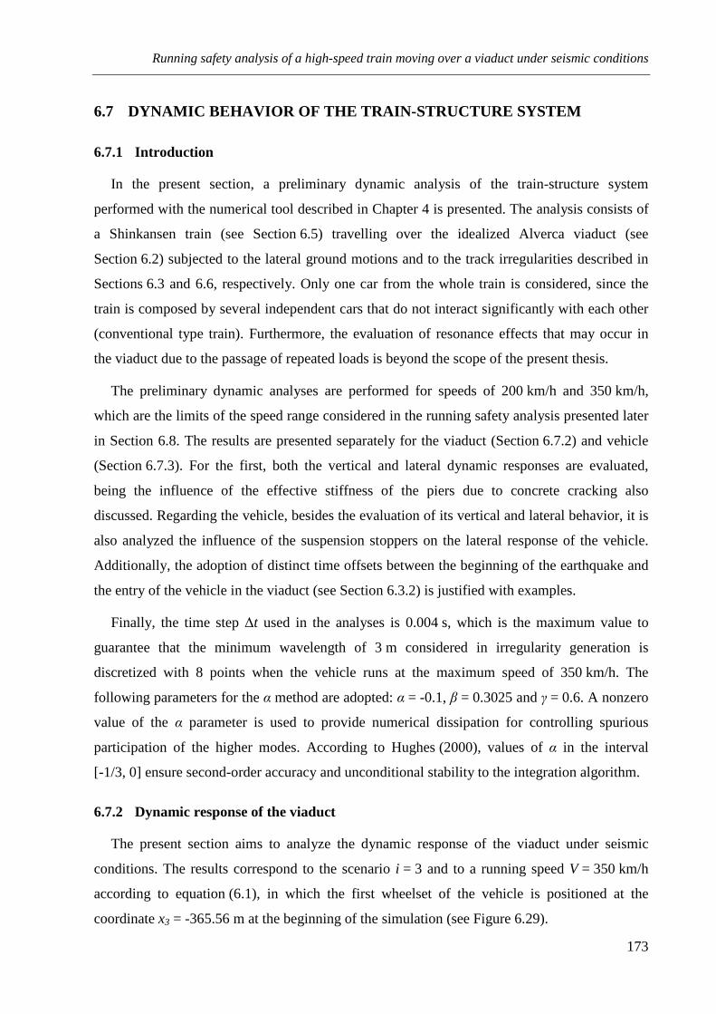
Running safety analysis of a high-speed train moving over a viaduct under seismic conditions
173
6.7 DYNAMIC BEHAVIOR OF THE TRAIN-STRUCTURE SYSTEM
6.7.1 Introduction
In the present section, a preliminary dynamic analysis of the train-structure system
performed with the numerical tool described in Chapter 4 is presented. The analysis consists of
a Shinkansen train (see Section 6.5) travelling over the idealized Alverca viaduct (see
Section 6.2) subjected to the lateral ground motions and to the track irregularities described in
Sections 6.3 and 6.6, respectively. Only one car from the whole train is considered, since the
train is composed by several independent cars that do not interact significantly with each other
(conventional type train). Furthermore, the evaluation of resonance effects that may occur in
the viaduct due to the passage of repeated loads is beyond the scope of the present thesis.
The preliminary dynamic analyses are performed for speeds of 200 km/h and 350 km/h,
which are the limits of the speed range considered in the running safety analysis presented later
in Section 6.8. The results are presented separately for the viaduct (Section 6.7.2) and vehicle
(Section 6.7.3). For the first, both the vertical and lateral dynamic responses are evaluated,
being the influence of the effective stiffness of the piers due to concrete cracking also
discussed. Regarding the vehicle, besides the evaluation of its vertical and lateral behavior, it is
also analyzed the influence of the suspension stoppers on the lateral response of the vehicle.
Additionally, the adoption of distinct time offsets between the beginning of the earthquake and
the entry of the vehicle in the viaduct (see Section 6.3.2) is justified with examples.
Finally, the time step ∆t used in the analyses is 0.004 s, which is the maximum value to
guarantee that the minimum wavelength of 3 m considered in irregularity generation is
discretized with 8 points when the vehicle runs at the maximum speed of 350 km/h. The
following parameters for the α method are adopted: α = -0.1, β = 0.3025 and γ = 0.6. A nonzero
value of the α parameter is used to provide numerical dissipation for controlling spurious
participation of the higher modes. According to Hughes (2000), values of α in the interval
[-1/3, 0] ensure second-order accuracy and unconditional stability to the integration algorithm.
6.7.2 Dynamic response of the viaduct
The present section aims to analyze the dynamic response of the viaduct under seismic
conditions. The results correspond to the scenario i = 3 and to a running speed V = 350 km/h
according to equation (6.1), in which the first wheelset of the vehicle is positioned at the
coordinate x3 = -365.56 m at the beginning of the simulation (see Figure 6.29).

Chapter 6
174
Figure 6.29 - Scenario i = 3 according to equation (6.1) for V = 350 km/h.
6.7.2.1 Vertical response
The vertical displacements of the deck at the midspan of the first span and 15th span (center
span) are plotted in Figure 6.30. The responses are obtained for two distinct scenarios: in the
first scenario (Figure 6.30a) the viaduct is subjected exclusively to the load of the vehicle
running at V = 350 km/h, while in the second scenario (Figure 6.30b) the viaduct is also
subjected to the seismic action with T = 310 years (see Section 6.3). On both scenarios, the
track quality corresponds to the regular operation limit (see Section 6.6). Since only the lateral
component of the earthquake is considered, the vertical response of the deck is not affected by
the seismic action. As a consequence, and also due to the fact that there is almost no continuity
between spans, the vertical excitation in each span is felt only when the vehicle crosses them. A
similar conclusion can be drawn from the vertical accelerations presented in Figure 6.31.
(a)
(b)
Figure 6.30 - Vertical displacements of the deck at the midspan of span 1 and 15 (V = 350 km/h):
(a) without earthquake and (b) subjected to the seismic action with T = 310 years.
. . .
. .
Viaduct edge
Viaduct length = 630 m
V = 350 km/hy
xgaɺɺ
.
x = -365.56 m3
0 2 4 6 8 10 12
−2
−1
0
1
2
Time (s)
Vertical displ. (mm) Span 1
Span 15
Vehicle at
midspan 1
Vehicle at
midspan 15
Vehicle over the viaduct
0 2 4 6 8 10 12
−2
−1
0
1
2
Time (s)
Vertical displ. (mm) Span 1
Span 15
Vehicle at
midspan 1
Vehicle at
midspan 15
Vehicle over the viaduct

Running safety analysis of a high-speed train moving over a viaduct under seismic conditions
175
(a)
(b)
Figure 6.31 - Vertical accelerations of the deck at the midspan of span 1 and 15 (V = 350 km/h):
(a) without earthquake and (b) subjected to the seismic action with T = 310 years.
6.7.2.2 Lateral response
Figures 6.32 and 6.33 show the lateral responses of the deck in terms of displacements (the
lateral displacement of the deck is relative to the lateral displacement at the base of the piers)
and accelerations, respectively, for the same scenario described above. Contrary to what is
observed in the vertical direction, the vehicle has a small influence in the lateral response of the
viaduct, since the lateral impacts that occur between the wheel and rail are barely reflected in
the deck response (the maximum displacement and acceleration is less than 0.10 mm and
0.15 m/s-2, respectively). It can also be observed, especially in the displacements, that the
response of the first span has a higher frequency and lower amplitude than the response of the
middle span. This is a consequence of the lower flexibility of the viaduct at the ends due to the
connection to the abutments. Although the bearing supports are the same in these locations as
in the rest of the viaduct, since the flexibility of the abutment and the surrounding embankment
is not considered in the model, the edge spans are considerably more constrained than the
others.
0 2 4 6 8 10 12
−2
−1
0
1
2
Time (s)
Span 1
Span 15
Vertical accel. (m.s−2)
Vehicle over the viaduct
Vehicle at
midspan 1
Vehicle at
midspan 15
0 2 4 6 8 10 12
−2
−1
0
1
2
Time (s)
Span 1
Span 15
Vertical accel. (m.s−2)
Vehicle at
midspan 1
Vehicle at
midspan 15
Vehicle over the viaduct

Chapter 6
176
(a)
(b)
Figure 6.32 - Lateral displacements of the deck at the midspan of span 1 and 15 (V = 350 km/h):
(a) without earthquake and (b) subjected to the seismic action with T = 310 years.
(a)
(b)
Figure 6.33 - Lateral accelerations of the deck at the midspan of span 1 and 15 (V = 350 km/h):
(a) without earthquake and (b) subjected to the seismic action with T = 310 years
0 2 4 6 8 10 12−0.10
−0.05
0.00
0.05
0.10
Time (s)
Lateral displ. (mm) Span 1
Span 15Vehicle over the viaduct
Vehicle at
midspan 1
Vehicle at
midspan 15
0 2 4 6 8 10 12
−20
−10
0
10
20
Time (s)
Lateral displ. (mm) Span 1
Span 15Vehicle over the viaduct
Vehicle at
midspan 1
Vehicle at
midspan 15
0 2 4 6 8 10 12−0.2
−0.1
0.0
0.1
0.2
Time (s)
Lateral accel. (m.s−2)
Span 1
Span 15Vehicle over the viaduct
Vehicle at
midspan 1
Vehicle at
midspan 15
0 2 4 6 8 10 12
−3.0
−1.5
0.0
1.5
3.0
Time (s)
Lateral accel. (m.s−2)
Span 1
Span 15Vehicle over the viaduct
Vehicle at
midspan 1
Vehicle at
midspan 15

Running safety analysis of a high-speed train moving over a viaduct under seismic conditions
177
6.7.2.3 Influence of the effective stiffness of the piers
As mentioned in Section 6.4, although the structure is not expected to experience significant
damage for the levels of seismicity considered in the present study, the reduction in the flexural
stiffness of the piers should be considered to account for concrete cracking. Therefore, the
present section aims to evaluate the effect of this procedure on the lateral response of the
viaduct.
The lateral displacements of the deck at the midspan of the 15th (center span) when the
viaduct is subjected to the vehicle load, running at V = 350 km/h, and to the seismic actions
with T = 95 years and T = 310 years are depicted in Figures 6.34 and 6.35, respectively. The
figures also show the response spectra of both accelerograms, together with the representation
of the shift in the structural period T due to the reduction in the flexural stiffness of the piers
(see Figures 6.5a and 6.19a for the frequencies f1 of the first mode of vibration of the viaduct
considering the elastic and the effective stiffness, respectively). The subscripts ela and eff
indicate elastic and effective stiffness. For both scenarios of seismicity, the frequency of the
response become lower after considering the effect of concrete cracking in the piers. On the
other hand, although the spectral acceleration decreases due to the increase in the period of the
structure (see Figures 6.34b and 6.35b), the amplitude of the response increases. This is due to
the fact that the piers are less stiff and therefore may experience larger displacements during
the earthquake.
(a) (b)
Figure 6.34 - Influence of the effective stiffness of the piers on the response of the structure for the
seismic action with T = 95 years: (a) lateral displacements of the deck at the midspan of span 15
and (b) shift in the structural period.
0 2 4 6 8 10 12−20
−15
−10
−5
0
5
10
15
20
25
Time (s)
Lateral displ. (mm)
Elastic stiffness
Effective stiffness
Vehicle over viaduct
0 1 2 3 40.0
1.0
2.0
3.0
4.0
Period (s)
Spec
tral
acc
eler
atio
n (
m.s
−2) Target spectrum EC8
Generated spectrum
Tela
= 0
.52
s (f 1
= 1
.93
Hz)
Teff =
0.7
9 s (f
1 =
1.2
7 H
z)

Chapter 6
178
(a) (b)
Figure 6.35 - Influence of the effective stiffness of the piers on the response of the structure for the
seismic action with T = 310 years: (a) lateral displacements of the deck at the midspan of span 15
and (b) shift in the structural period.
6.7.3 Dynamic response of the vehicle
The present section aims to assess the dynamic behavior of the Shinkansen high-speed train
when travelling on the railway viaduct under seismic conditions. All the results, with the
exception of Section 6.7.3.4, correspond to the scenario i = 3 according to equation (6.1), in
which the first wheelset of the vehicle is positioned at the coordinate x3 = -73.89 m or
x3 = -365.56 m at the beginning of the simulation for speeds of 200 and 350 km/h, respectively
(see Figure 6.29). In Section 6.7.3.4 the influence of the time offset between the beginning of
the earthquake and the entry of the vehicle in the viaduct is discussed, using as an example the
scenarios i = 1, i = 2, i = 3 and i = 4 (see equation (6.1))
6.7.3.1 Vertical response
Figure 6.36 shows the vertical accelerations at the center of mass of the carbody and second
wheelset calculated for speeds of 200 km/h and 350 km/h. On both scenarios the track quality
corresponds to the regular operation limit and, since the earthquake does not influence the
vertical response of the system (see Section 6.7.2.1), no seismic action is considered. It is
perfectly clear that the frequency of the acceleration response of the carbody is much lower
than that of the wheelset, which demonstrates the efficiency of the suspensions on filtering the
high frequencies arising from the contact between wheel and rail. Regarding the amplitude, the
differences are more pronounced when the vehicle runs at higher speeds, since the influence of
0 2 4 6 8 10 12−20
−15
−10
−5
0
5
10
15
20
25
Time (s)
Lateral displ. (mm)
Elastic stiffness
Effective stiffness
Vehicle over viaduct
0 1 2 3 40.0
1.0
2.0
3.0
4.0
Period (s)
Sp
ectr
al a
ccel
erat
ion
(m
.s−
2) Target spectrum EC8
Generated spectrum
Tela
= 0
.52
s (f1 =
1.9
3 H
z)
Teff =
0.7
9 s (f1
= 1
.27
Hz)
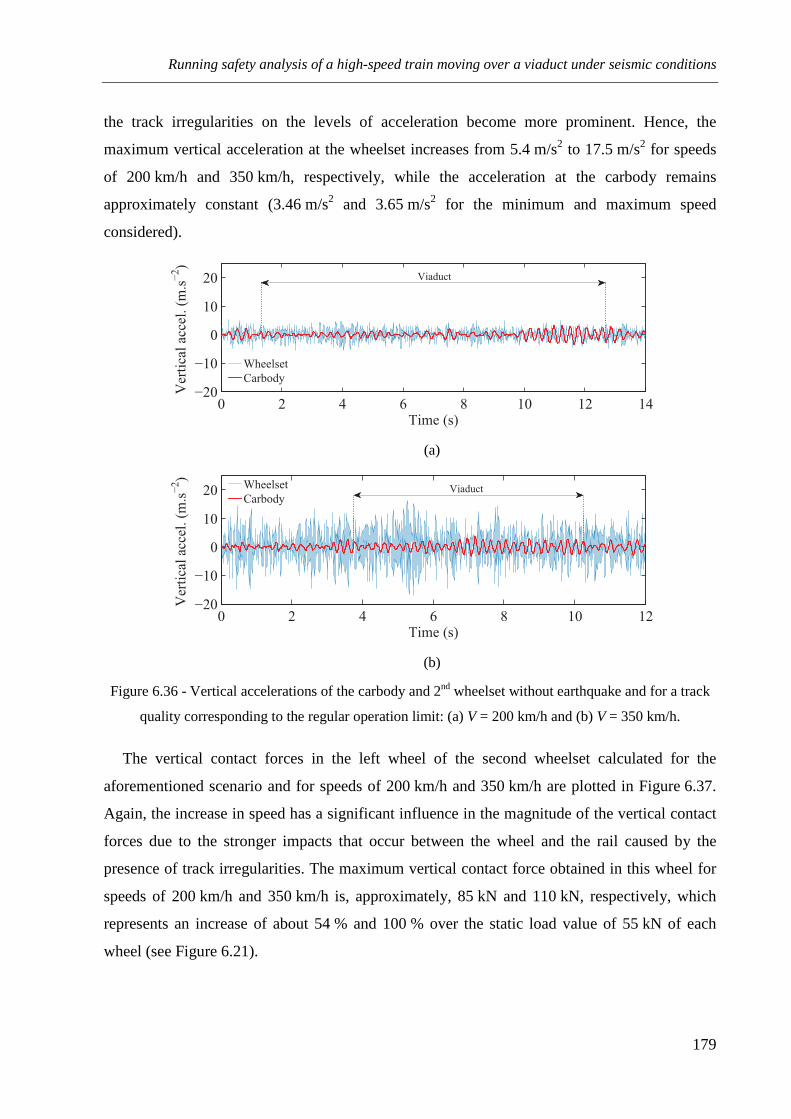
Running safety analysis of a high-speed train moving over a viaduct under seismic conditions
179
the track irregularities on the levels of acceleration become more prominent. Hence, the
maximum vertical acceleration at the wheelset increases from 5.4 m/s2 to 17.5 m/s2 for speeds
of 200 km/h and 350 km/h, respectively, while the acceleration at the carbody remains
approximately constant (3.46 m/s2 and 3.65 m/s2 for the minimum and maximum speed
considered).
(a)
(b)
Figure 6.36 - Vertical accelerations of the carbody and 2nd wheelset without earthquake and for a track
quality corresponding to the regular operation limit: (a) V = 200 km/h and (b) V = 350 km/h.
The vertical contact forces in the left wheel of the second wheelset calculated for the
aforementioned scenario and for speeds of 200 km/h and 350 km/h are plotted in Figure 6.37.
Again, the increase in speed has a significant influence in the magnitude of the vertical contact
forces due to the stronger impacts that occur between the wheel and the rail caused by the
presence of track irregularities. The maximum vertical contact force obtained in this wheel for
speeds of 200 km/h and 350 km/h is, approximately, 85 kN and 110 kN, respectively, which
represents an increase of about 54 % and 100 % over the static load value of 55 kN of each
wheel (see Figure 6.21).
0 2 4 6 8 10 12 14−20
−10
0
10
20
Time (s)
Vertical accel. (m.s−2)
Wheelset
Carbody
Viaduct
0 2 4 6 8 10 12−20
−10
0
10
20
Time (s)
Vertical accel. (m.s−2)
Wheelset
CarbodyViaduct

Chapter 6
180
(a)
(b)
Figure 6.37 - Vertical contact forces in the left wheel of the 2nd wheelset without earthquake and for a
track quality corresponding to the regular operation limit: (a) V = 200 km/h and (b) V = 350 km/h.
6.7.3.2 Lateral response
The lateral displacements at the center of mass of the carbody and second wheelset are
plotted in Figure 6.38 (the displacements of the vehicle are relative to the lateral displacement
of the track centerline). The responses are obtained for two distinct scenarios: in the first
scenario (Figure 6.38a) the viaduct is subjected exclusively to the load of the vehicle running at
V = 350 km/h, while in the second scenario (Figure 6.38b) the viaduct is also subjected to the
seismic action with T =310 years. On both scenarios, the track irregularities correspond to the
regular operation limit. By comparing Figure 6.38a with Figure 6.38b, it is clear that the
earthquake is the main responsible for the large lateral displacements experienced by the
carbody, since the track irregularities barely contribute to them, as it can be observed in
Figure 6.38a. Under seismic conditions, the maximum lateral displacement of the carbody,
relative to the lateral displacement of the track centerline, is approximately six times higher
than the maximum displacement of the wheelset.
0 2 4 6 8 10 12 140
25
50
75
100
125
Time (s)
Ver
tica
l fo
rce
(kN
)
Dynamic
Static
Viaduct
0 2 4 6 8 10 120
25
50
75
100
125
Time (s)
Ver
tica
l fo
rce
(kN
) Dynamic
StaticViaduct
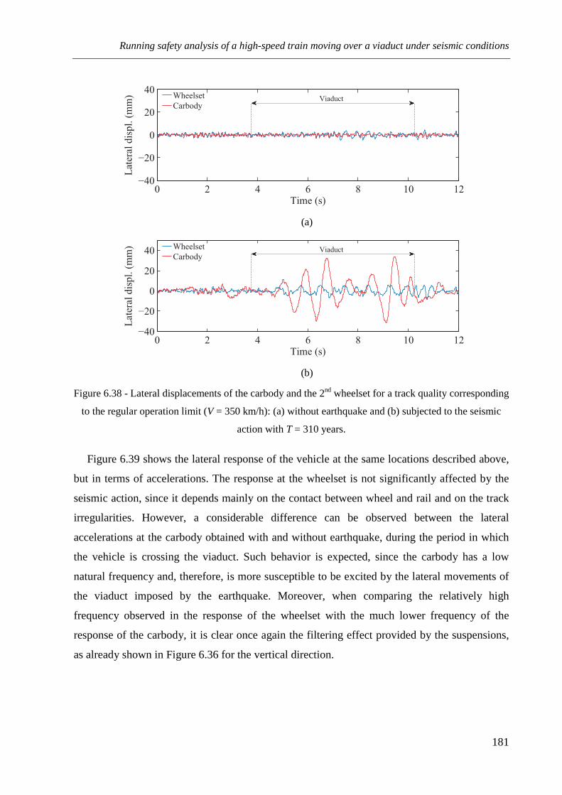
Running safety analysis of a high-speed train moving over a viaduct under seismic conditions
181
(a)
(b)
Figure 6.38 - Lateral displacements of the carbody and the 2nd wheelset for a track quality corresponding
to the regular operation limit (V = 350 km/h): (a) without earthquake and (b) subjected to the seismic
action with T = 310 years.
Figure 6.39 shows the lateral response of the vehicle at the same locations described above,
but in terms of accelerations. The response at the wheelset is not significantly affected by the
seismic action, since it depends mainly on the contact between wheel and rail and on the track
irregularities. However, a considerable difference can be observed between the lateral
accelerations at the carbody obtained with and without earthquake, during the period in which
the vehicle is crossing the viaduct. Such behavior is expected, since the carbody has a low
natural frequency and, therefore, is more susceptible to be excited by the lateral movements of
the viaduct imposed by the earthquake. Moreover, when comparing the relatively high
frequency observed in the response of the wheelset with the much lower frequency of the
response of the carbody, it is clear once again the filtering effect provided by the suspensions,
as already shown in Figure 6.36 for the vertical direction.
0 2 4 6 8 10 12−40
−20
0
20
40
Time (s)
Lateral displ. (mm) Wheelset
CarbodyViaduct
0 2 4 6 8 10 12−40
−20
0
20
40
Time (s)
Lateral displ. (mm) Wheelset
CarbodyViaduct

Chapter 6
182
(a)
(b)
Figure 6.39 - Lateral accelerations of the carbody and the 2nd wheelset for a track quality corresponding
to the regular operation limit (V = 350 km/h): (a) without earthquake and (b) subjected to the seismic
action with T = 310 years.
Finally, the lateral contact forces obtained in the left wheel of the second wheelset for
speeds of 200 km/h and 350 km/h are plotted in Figures 6.40 and 6.41, respectively. On both
figures, the lateral contact forces are superimposed on the relative lateral displacements
between wheel and rail. It is clear that the peaks observed in the lateral contact forces during
the earthquake are due to the wheel flange impacts, since they occur at the same moment as the
gap between the flange and rail closes (approximately 6 mm). This is particularly noticeable in
Figure 6.41b. When the viaduct is not subjected to any ground motion, the excitations caused
solely by the track irregularities are not sufficient to cause lateral impacts between the flange
and the rail, leading to a decrease in the levels of contact force. Figure 6.42 illustrates, as an
example, the relative position between the wheel and the rail at the instant indicated in
Figure 6.41 (t = 5.7 s). As expected, in the scenario where the viaduct is not subjected to any
ground motion, the flange is still far from the rail and no impact occurs, while in the scenario in
which the earthquake action is considered the impact is perfectly visible.
0 2 4 6 8 10 12−20
−10
0
10
20
Time (s)
Lateral accel. (m.s−2)
Wheelset
CarbodyViaduct
0 2 4 6 8 10 12−20
−10
0
10
20
Time (s)
Lateral accel. (m.s−2)
Wheelset
CarbodyViaduct

Running safety analysis of a high-speed train moving over a viaduct under seismic conditions
183
(a)
(b)
Figure 6.40 - Lateral contact forces and displacements of the left wheel of the second wheelset
(V = 200 km/h): (a) without earthquake and (b) subjected to the seismic action with T = 310 years.
(a)
(b)
Figure 6.41 - Lateral contact forces and displacements of the left wheel of the 2nd wheelset
(V = 350 km/h): (a) without earthquake and (b) subjected to the seismic action with T = 310 years.
0 2 4 6 8 10 12 14−20
−10
0
10
20
30
40
Time (s)
Lateral force (kN) Force
Displacement
−5
0
5
10
15
Lateral displ. (mm)
Viaduct
Flange gap
0 2 4 6 8 10 12 14−20
−10
0
10
20
30
40
Time (s)
Lateral force (kN) Force
Displacement
−5
0
5
10
15
Lateral displ. (mm)
Flange gap
Viaduct
0 2 4 6 8 10 12−20
−10
0
10
20
30
40
Time (s)
Lateral force (kN) Force
Displacement
−5
0
5
10
15
Lateral displ. (mm)Viaduct
Flange gapFigure 6.41a
0 2 4 6 8 10 12−20
−10
0
10
20
30
40
Time (s)
Lateral force (kN) Force
Displacement
−5
0
5
10
15
Lateral displ. (mm)Viaduct
Flange gapFigure 6.41b

Chapter 6
184
(a) (b)
Figure 6.42 - Relative position between the left wheel of the 2nd wheelset and rail at t = 5.7 s
(V = 350 km/h): (a) without earthquake and (b) subjected to the seismic action with T = 310 years.
6.7.3.3 Influence of the suspension stoppers
Most of the high-speed trains have stoppers installed in the secondary transversal
suspensions in order to avoid large lateral displacements of the carbody, especially during
earthquake. These devices are characterized by a multilinear force-displacement law that
simulates the presence of a rubber pad whose stiffness increases gradually (see Section 6.5.2).
Thus, although the importance of the stoppers is unquestionable during intense earthquakes, the
present section aims to evaluate if they also influence the behavior of the carbody in the
presence of moderate seismic actions as those considered in this work.
The lateral displacements of the carbody at a point above the first bogie relative to the
displacements of the center of mass of the first bogie are depicted in Figure 6.43a. The response
is obtained for a scenario in which the vehicle runs on the viaduct at V = 350 km/h, subjected to
the seismic action with T =310 years and to the track irregularities corresponding to the regular
operation limit. In order to evaluate the influence of the stopper on the response of the carbody,
the displacements of the actual vehicle are compared with those obtained for the same vehicle
but without the presence of this device, i.e., with a secondary lateral suspension characterized
by a linear force-displacement law equivalent to the initial stretch of the actual suspension, as
shown in Figure 6.43b3. It can be observed that the maximum relative displacement δmax
3 As mentioned in Section 6.5, the geometrical and mechanical properties of the Shinkansen train cannot be published due to confidential matters from the manufacturer. Therefore, no details about the multilinear suspension law are given in Figures 6.43b and 6.44b.
−60 −30 0 30 60 90−40
−30
−20
−10
0
10
20
y (mm)
z (m
m)
Tread contactWheel
Rail
−60 −30 0 30 60 90−40
−30
−20
−10
0
10
20
y (mm)
z (m
m)
Wheel
Rail
Flange impact
Tread contact

Running safety analysis of a high-speed train moving over a viaduct under seismic conditions
185
between the carbody and the bogie is around 33 mm, which is already above the linear
threshold value of 22 mm of the multilinear law. However, although it is notable that the
responses start to diverge from each other after the threshold value is reached, the maximum
displacements do not show considerable differences. This is due to the fact that the increase in
the suspension's stiffness is still not significant for the levels of displacements experienced by
the carbody, as can be seen in Figure 6.43b. Thus, for the levels of seismic intensity studied in
the present work, the stoppers do not have an important impact in the lateral response of the
vehicle.
(a) (b)
Figure 6.43 - Multilinear vs. Linear law of the secondary transversal suspension: (a) lateral response of
the carbody and (b) force-displacement laws of the suspension.
Nevertheless, in order to demonstrate the behavior of the stopper in a situation in which the
carbody would experience the impact with the stiff rubber pad, a comparison between the
response of the carbody with the actual suspension and with a suspension characterized by a
bilinear law whose first and second stretches are equivalent to the first and last stretches of the
actual suspension is depicted in Figure 6.44. While in the scenario represented in Figure 6.43
the stiffness of the linear suspension is about 65 % of the value of the actual suspension's
stiffness for δmax = 33 mm, in the scenario depicted in Figure 6.44, the stiffness of the bilinear
suspension for the same level of displacements is around 265 % of the value of the actual
stiffness. Consequently, the sudden increase in stiffness provided by the suspension with a
bilinear law significantly restrains the lateral displacements of the carbody, thus demonstrating
the importance of these devices in maintaining the stability of the vehicle.
0 2 4 6 8 10 12−40
−20
0
20
40
Time (s)
Lateral displ. (mm)
Multilinear law
Linear law
Viaduct
Linear treshold
−50 −25 0 25 50−40
−30
−20
−10
0
10
20
30
40
Displacement (mm)
Fo
rce
(kN
)
Multilinear law
Linear law
Lin
ear
tres
hold
Lin
ear
tres
hold
max
δ
max
33m
mδ≃
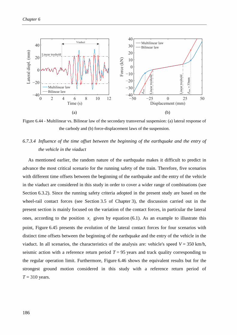
Chapter 6
186
(a) (b)
Figure 6.44 - Multilinear vs. Bilinear law of the secondary transversal suspension: (a) lateral response of
the carbody and (b) force-displacement laws of the suspension.
6.7.3.4 Influence of the time offset between the beginning of the earthquake and the entry of
the vehicle in the viaduct
As mentioned earlier, the random nature of the earthquake makes it difficult to predict in
advance the most critical scenario for the running safety of the train. Therefore, five scenarios
with different time offsets between the beginning of the earthquake and the entry of the vehicle
in the viaduct are considered in this study in order to cover a wider range of combinations (see
Section 6.3.2). Since the running safety criteria adopted in the present study are based on the
wheel-rail contact forces (see Section 3.5 of Chapter 3), the discussion carried out in the
present section is mainly focused on the variation of the contact forces, in particular the lateral
ones, according to the position ix given by equation (6.1). As an example to illustrate this
point, Figure 6.45 presents the evolution of the lateral contact forces for four scenarios with
distinct time offsets between the beginning of the earthquake and the entry of the vehicle in the
viaduct. In all scenarios, the characteristics of the analysis are: vehicle's speed V = 350 km/h,
seismic action with a reference return period T = 95 years and track quality corresponding to
the regular operation limit. Furthermore, Figure 6.46 shows the equivalent results but for the
strongest ground motion considered in this study with a reference return period of
T = 310 years.
0 2 4 6 8 10 12−40
−20
0
20
40
Time (s)
Lateral displ. (mm)
Multilinear law
Bilinear law
Viaduct
Linear treshold
−50 −25 0 25 50−40
−30
−20
−10
0
10
20
30
40
Displacement (mm)
Forc
e (k
N)
Multilinear law
Bilinear law
Lin
ear
tres
hold
Lin
ear
tres
hold
max
δ
max
33m
mδ≃

Running safety analysis of a high-speed train moving over a viaduct under seismic conditions
187
(a) Coordinate x1 for the scenario i = 1
(b) Coordinate x2 for the scenario i = 2
(c) Coordinate x3 for the scenario i = 3
(d) Coordinate x4 for the scenario i = 4
Figure 6.45 - Lateral contact forces in the left wheel of the 2nd wheelset for the seismic action with
T = 95 years, track quality corresponding to the regular operation limit and V = 350 km/h: Coordinates
of the first wheelset according to equation (6.1): (a) x1, (b) x2, (c) x3 and (d) x4.
0 2 4 6 8 10 12 14 16 18 20
−20
−10
0
10
20
30
40
Time (s)
Lateral force (kN) Viaduct
Earthquake
0 2 4 6 8 10 12 14 16
−20
−10
0
10
20
30
40
Time (s)
Lateral force (kN) Viaduct
Earthquake
0 2 4 6 8 10 12
−20
−10
0
10
20
30
40
Time (s)
Lateral force (kN) Viaduct
Earthquake. . .
0 2 4 6 8
−20
−10
0
10
20
30
40
Time (s)
Lateral force (kN) Viaduct
Earthquake. . .

Chapter 6
188
(a) Coordinate x1 for the scenario i = 1
(b) Coordinate x2 for the scenario i = 2
(c) Coordinate x3 for the scenario i = 3
(d) Coordinate x4 for the scenario i = 4
Figure 6.46 - Lateral contact forces in the left wheel of the 2nd wheelset for the seismic action with
T = 310 years, track quality corresponding to the regular operation limit and V = 350 km/h: Coordinates
of the first wheelset according to equation (6.1): (a) x1, (b) x2, (c) x3 and (d) x4.
0 2 4 6 8 10 12 14 16 18 20
−20
−10
0
10
20
30
40
Time (s)
Lateral force (kN) Viaduct
Earthquake
0 2 4 6 8 10 12 14 16
−20
−10
0
10
20
30
40
Time (s)
Lateral force (kN) Viaduct
Earthquake
0 2 4 6 8 10 12
−20
−10
0
10
20
30
40
Time (s)
Lateral force (kN) Viaduct
Earthquake. . .
0 2 4 6 8
−20
−10
0
10
20
30
40
Time (s)
Lateral force (kN) Viaduct
Earthquake. . .

Running safety analysis of a high-speed train moving over a viaduct under seismic conditions
189
As expected, the most critical scenario is not the same for the two situations depicted in
Figures 6.45 and 6.46, since the maximum lateral contact force for the seismic action with
T = 310 years occurs in the scenario presented in Figure 6.46b (44.5 kN), while for the seismic
action with T = 95 years this scenario is one of the least conditioning with a maximum lateral
force of 17.8 kN. Similar conclusions were drawn for all other scenarios, i.e., the random
nature of the seismic action, together with the vast number of possible combinations regarding
the time offset between the start of the earthquake and the entry of the vehicle in the viaduct,
makes it very difficult to find a unique scenario that could be representative of all possible
situations. Therefore, in the running safety study presented in Section 6.8, the outcome of each
analysis is the result of the envelope obtained in the five scenarios presented in Section 6.3.2.
Nevertheless, a stochastic approach of the problem would be necessary to obtain a more
representative range of results.
6.8 RUNNING SAFETY ANALYSIS
6.8.1 Introduction
In the present section, the running safety analysis of one of the Shinkansen cars travelling
over the idealized Alverca viaduct under seismic conditions is assessed. As mentioned in
Section 6.7, the use of only one car is adequate for the purpose of evaluating the running safety,
since the Shinkansen is a conventional type train whose cars do not significantly interact with
each other.
For each level of seismic intensity and track irregularity described in Sections 6.3 and 6.6,
respectively, the dynamic analyses are performed for speeds ranging from 200 km/h to
350 km/h with steps of 10 km/h. Furthermore, for each speed, five scenarios are considered to
account for the time offset between the beginning of the earthquake and the entry of the vehicle
in the viaduct, as described in Section 6.3.2. In each scenario, the circulation is considered to be
safe as long as none of the safety criteria described in Section 3.5 of Chapter 3 is violated
during the whole time that the vehicle is crossing the viaduct. Regarding the derailment due to
wheel flange climbing, only the modified Nadal criterion based on the lateral impact duration is
used (See Section 3.5.1.4 of Chapter 3).
The time integration parameters adopted for the solution of the dynamic equations of motion
of the train-structure system are the same as those considered in Section 6.7. All the analyses
finish 2 seconds after the vehicle leaves the viaduct.

Chapter 6
190
6.8.2 Influence of the seismic intensity level
The maximum values of the safety criteria obtained for each seismic intensity level in a
scenario in which the vehicle crosses the viaduct at 350 km/h with a track quality
corresponding to the regular operation limit are listed in Table 6.6. The values presented in this
table correspond to an envelope of results regarding all the five scenarios described in
Section 6.3.2 and all the wheels of the vehicle. While the Nadal, Prud'homme and rail roll
criteria, which depend on the Y/Q ratio or on the lateral contact force solely, are significantly
affected by the earthquake intensity, the wheel unloading criterion, which depends exclusively
on the vertical contact forces, shows less variation. This is due to the fact that only the lateral
component of the earthquake is accounted.
In the present scenario, the risk of derailment is null for levels of seismicity corresponding
to earthquakes with return periods up to 95 years. Above this level, at least one out of the four
criteria is not satisfied. Note that, according to these criteria, the safety of the vehicle may be at
risk for levels of seismicity around three times less than the level of the design seismic action
defined by the EN 1998-1 (2004) (the reference return period associated with the design
seismic action is 475 years). Thus, the results show that the train's safety might be jeopardized
even if the structure does not suffer significant damage during the earthquake.
Table 6.6 - Maximum values of the safety criteria for different seismic intensities.
T (years) Modified Nadal Prud'homme Rail roll Wheel unloading
No earthquake 0.26 0.37 0.16 0.72
95 0.71 0.89 0.41 0.76
150 0.70 1.17 0.69 0.82
225 1.02 1.35 0.69 0.89
310 1.05 1.42 0.72 0.90
As an example to clarify the present discussion, the time-histories of the four safety criteria
obtained in the aforementioned scenario for the four seismic intensities considered in this study
are plotted in Figures 6.47 to 6.50. All the results correspond to the scenario 2=i according to
equation (6.1). The Nadal and wheel unloading criteria correspond to the left wheel of the
second wheelset, while the Prud'homme and rail roll criteria are related to the second wheelset
and to the left side of the first bogie, respectively. As it can be observed, the Nadal,
Prud'homme and rail roll criteria are significantly dependent on the seismic action when the
vehicle is crossing the viaduct, while the wheel unloading criterion is barely affected.

Running safety analysis of a high-speed train moving over a viaduct under seismic conditions
191
(a) T = 95 years
(b) T = 150 years
(c) T = 225 years
(d) T = 310 years
Figure 6.47 - Nadal factor relative to the left wheel of the 2nd wheelset for the scenario i = 2
(equation (6.1)), V = 350 km/h and track quality corresponding to the regular operation limit.
0 2 4 6 8 10 12 14 160.0
0.2
0.4
0.6
0.8
1.0
1.2
Time (s)
Nad
al f
acto
rN
ζ
Viaduct
Safety limit
0 2 4 6 8 10 12 14 160.0
0.2
0.4
0.6
0.8
1.0
1.2
Time (s)
Nad
al f
acto
rN
ζ
Viaduct
Safety limit
0 2 4 6 8 10 12 14 160.0
0.2
0.4
0.6
0.8
1.0
1.2
Time (s)
Nad
al f
acto
rN
ζ
Viaduct
Safety limit
0 2 4 6 8 10 12 14 160.0
0.2
0.4
0.6
0.8
1.0
1.2
Time (s)
Nad
al f
acto
rN
ζ
Viaduct
Safety limit

Chapter 6
192
(a) T = 95 years
(b) T = 150 years
(c) T = 225 years
(d) T = 310 years
Figure 6.48 - Prud'homme factor relative to the 2nd wheelset for the scenario i = 2 (equation (6.1)),
V = 350 km/h and track quality corresponding to the regular operation limit.
0 2 4 6 8 10 12 14 160.00
0.25
0.50
0.75
1.00
1.25
1.50
Time (s)
Pru
d’h
om
me
fact
or
Pζ Viaduct
Safety limit
0 2 4 6 8 10 12 14 160.00
0.25
0.50
0.75
1.00
1.25
1.50
Time (s)
Pru
d’h
om
me
fact
or
Pζ Viaduct
Safety limit
0 2 4 6 8 10 12 14 160.00
0.25
0.50
0.75
1.00
1.25
1.50
Time (s)
Pru
d’h
om
me
fact
or
Pζ Viaduct
Safety limit
0 2 4 6 8 10 12 14 160.00
0.25
0.50
0.75
1.00
1.25
1.50
Time (s)
Pru
d’h
om
me
fact
or
Pζ Viaduct
Safety limit
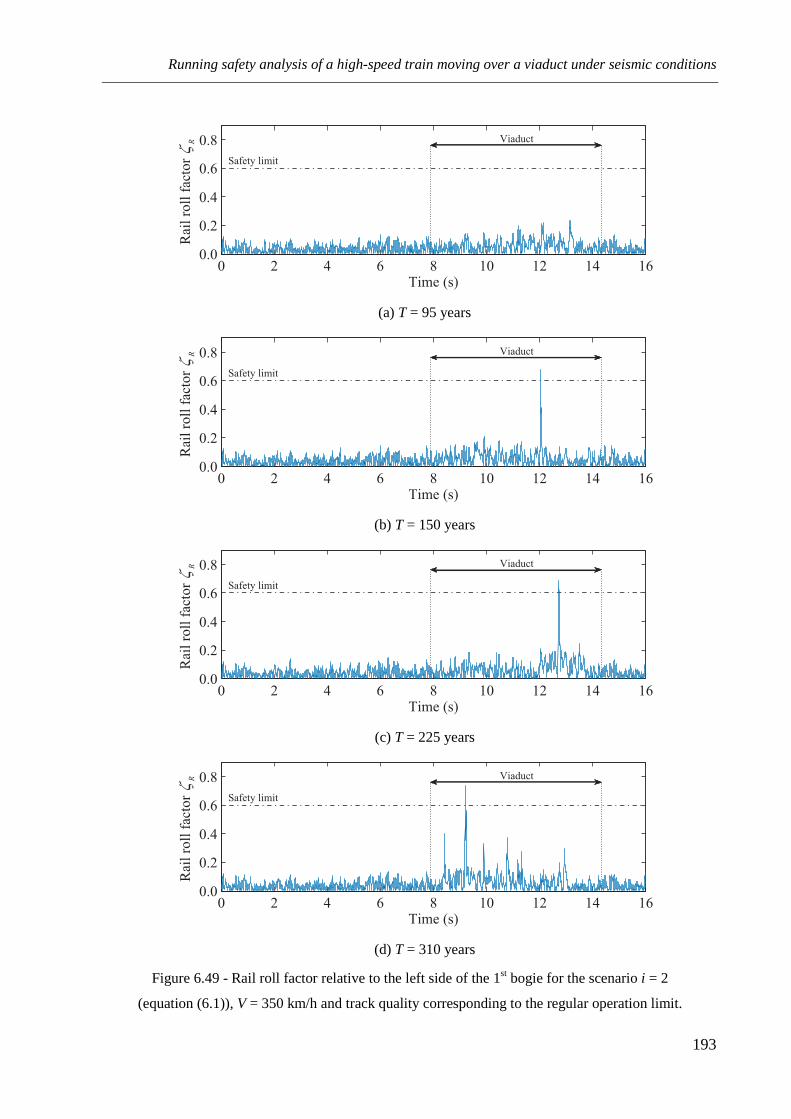
Running safety analysis of a high-speed train moving over a viaduct under seismic conditions
193
(a) T = 95 years
(b) T = 150 years
(c) T = 225 years
(d) T = 310 years
Figure 6.49 - Rail roll factor relative to the left side of the 1st bogie for the scenario i = 2
(equation (6.1)), V = 350 km/h and track quality corresponding to the regular operation limit.
0 2 4 6 8 10 12 14 160.0
0.2
0.4
0.6
0.8
Time (s)
Rai
l ro
ll f
acto
rR
ζ
Viaduct
Safety limit
0 2 4 6 8 10 12 14 160.0
0.2
0.4
0.6
0.8
Time (s)
Rai
l ro
ll f
acto
rR
ζ
Viaduct
Safety limit
0 2 4 6 8 10 12 14 160.0
0.2
0.4
0.6
0.8
Time (s)
Rai
l ro
ll f
acto
rR
ζ
Viaduct
Safety limit
0 2 4 6 8 10 12 14 160.0
0.2
0.4
0.6
0.8
Time (s)
Rai
l ro
ll f
acto
rR
ζ
Viaduct
Safety limit

Chapter 6
194
(a) T = 95 years
(b) T = 150 years
(c) T = 225 years
(d) T = 310 years
Figure 6.50 - Unloading factor relative to the left wheel of the 2nd wheelset for the scenario i = 2
(equation (6.1)), V = 350 km/h and track quality corresponding to the regular operation limit.
0 2 4 6 8 10 12 14 16−0.90
−0.45
0.00
0.45
0.90
1.35
1.80
Time (s)
Wheel unload factor
Uζ Viaduct
Safety limit
0 2 4 6 8 10 12 14 16−0.90
−0.45
0.00
0.45
0.90
1.35
1.80
Time (s)
Wheel unload factor
Uζ Viaduct
Safety limit
0 2 4 6 8 10 12 14 16−0.90
−0.45
0.00
0.45
0.90
1.35
1.80
Time (s)
Wheel unload factor
Uζ Viaduct
Safety limit
0 2 4 6 8 10 12 14 16−0.90
−0.45
0.00
0.45
0.90
1.35
1.80
Time (s)
Wheel unload factor
Uζ Viaduct
Safety limit
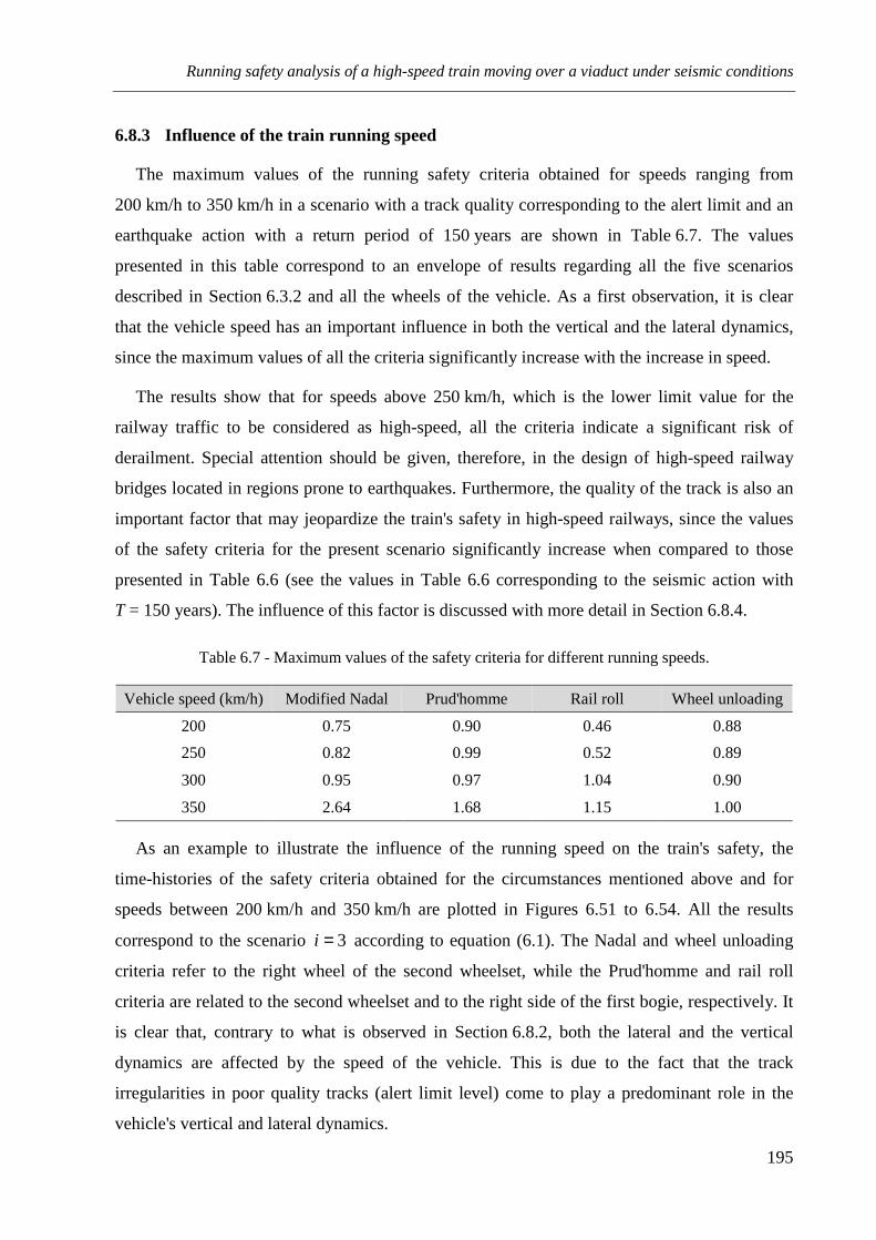
Running safety analysis of a high-speed train moving over a viaduct under seismic conditions
195
6.8.3 Influence of the train running speed
The maximum values of the running safety criteria obtained for speeds ranging from
200 km/h to 350 km/h in a scenario with a track quality corresponding to the alert limit and an
earthquake action with a return period of 150 years are shown in Table 6.7. The values
presented in this table correspond to an envelope of results regarding all the five scenarios
described in Section 6.3.2 and all the wheels of the vehicle. As a first observation, it is clear
that the vehicle speed has an important influence in both the vertical and the lateral dynamics,
since the maximum values of all the criteria significantly increase with the increase in speed.
The results show that for speeds above 250 km/h, which is the lower limit value for the
railway traffic to be considered as high-speed, all the criteria indicate a significant risk of
derailment. Special attention should be given, therefore, in the design of high-speed railway
bridges located in regions prone to earthquakes. Furthermore, the quality of the track is also an
important factor that may jeopardize the train's safety in high-speed railways, since the values
of the safety criteria for the present scenario significantly increase when compared to those
presented in Table 6.6 (see the values in Table 6.6 corresponding to the seismic action with
T = 150 years). The influence of this factor is discussed with more detail in Section 6.8.4.
Table 6.7 - Maximum values of the safety criteria for different running speeds.
Vehicle speed (km/h) Modified Nadal Prud'homme Rail roll Wheel unloading
200 0.75 0.90 0.46 0.88
250 0.82 0.99 0.52 0.89
300 0.95 0.97 1.04 0.90
350 2.64 1.68 1.15 1.00
As an example to illustrate the influence of the running speed on the train's safety, the
time-histories of the safety criteria obtained for the circumstances mentioned above and for
speeds between 200 km/h and 350 km/h are plotted in Figures 6.51 to 6.54. All the results
correspond to the scenario 3=i according to equation (6.1). The Nadal and wheel unloading
criteria refer to the right wheel of the second wheelset, while the Prud'homme and rail roll
criteria are related to the second wheelset and to the right side of the first bogie, respectively. It
is clear that, contrary to what is observed in Section 6.8.2, both the lateral and the vertical
dynamics are affected by the speed of the vehicle. This is due to the fact that the track
irregularities in poor quality tracks (alert limit level) come to play a predominant role in the
vehicle's vertical and lateral dynamics.

Chapter 6
196
(a) V = 200 km/h
(b) V = 250 km/h
(c) V = 300 km/h
(d) V = 350 km/h
Figure 6.51 - Nadal factor relative to the right wheel of the 2nd wheelset for the scenario i = 3
(equation (6.1)), seismic action with T = 150 years and track quality corresponding to the alert limit.
0 2 4 6 8 10 12 140.0
0.2
0.4
0.6
0.8
1.0
1.2
Time (s)
Nad
al f
acto
rN
ζViaduct
Safety limit
0 2 4 6 8 10 120.0
0.2
0.4
0.6
0.8
1.0
1.2
Time (s)
Nad
al f
acto
rN
ζ
Viaduct
Safety limit
0 2 4 6 8 10 120.0
0.2
0.4
0.6
0.8
1.0
1.2
Time (s)
Nad
al f
acto
rN
ζ
Viaduct
Safety limit
0 2 4 6 8 10 120.0
0.2
0.4
0.6
0.8
1.0
1.2
Time (s)
Nad
al f
acto
rN
ζ
Viaduct
Safety limit

Running safety analysis of a high-speed train moving over a viaduct under seismic conditions
197
(a) V = 200 km/h
(b) V = 250 km/h
(c) V = 300 km/h
(d) V = 350 km/h
Figure 6.52 - Prud'homme factor relative to the 2nd wheelset for the scenario i = 3 (equation (6.1)),
seismic action with T = 150 years and track quality corresponding to the alert limit.
0 2 4 6 8 10 12 140.00
0.25
0.50
0.75
1.00
1.25
1.50
Time (s)
Viaduct
Safety limit
Pru
d’h
om
me
fact
or
Pζ
0 2 4 6 8 10 120.00
0.25
0.50
0.75
1.00
1.25
1.50
Time (s)
Pru
d’h
om
me
fact
or
Pζ Viaduct
Safety limit
0 2 4 6 8 10 120.00
0.25
0.50
0.75
1.00
1.25
1.50
Time (s)
Pru
d’h
om
me
fact
or
Pζ Viaduct
Safety limit
0 2 4 6 8 10 120.00
0.25
0.50
0.75
1.00
1.25
1.50
Time (s)
Pru
d’h
om
me
fact
or
Pζ Viaduct
Safety limit

Chapter 6
198
(a) V = 200 km/h
(b) V = 250 km/h
(c) V = 300 km/h
(d) V = 350 km/h
Figure 6.53 - Rail roll factor relative to the right side of the 1st bogie for the scenario i = 3
(equation (6.1)), seismic action with T = 150 years and track quality corresponding to the alert limit.
0 2 4 6 8 10 12 140.0
0.2
0.4
0.6
0.8
Time (s)
Viaduct
Safety limitR
ail
roll
fac
tor
Rζ
0 2 4 6 8 10 120.0
0.2
0.4
0.6
0.8
Time (s)
Rai
l ro
ll f
acto
rR
ζ
Viaduct
Safety limit
0 2 4 6 8 10 120.0
0.2
0.4
0.6
0.8
Time (s)
Rai
l ro
ll f
acto
rR
ζ
Viaduct
Safety limit
0 2 4 6 8 10 120.0
0.2
0.4
0.6
0.8
Time (s)
Rai
l ro
ll f
acto
rR
ζ
Viaduct
Safety limit
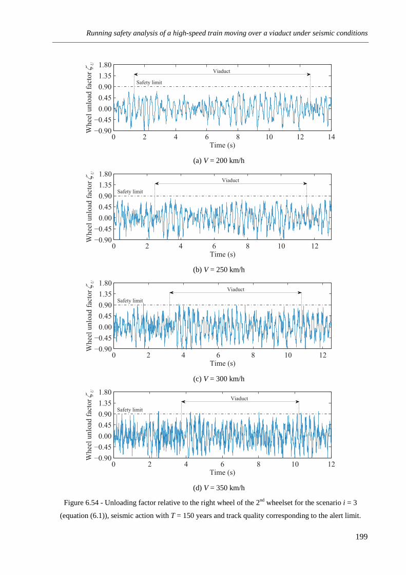
Running safety analysis of a high-speed train moving over a viaduct under seismic conditions
199
(a) V = 200 km/h
(b) V = 250 km/h
(c) V = 300 km/h
(d) V = 350 km/h
Figure 6.54 - Unloading factor relative to the right wheel of the 2nd wheelset for the scenario i = 3
(equation (6.1)), seismic action with T = 150 years and track quality corresponding to the alert limit.
0 2 4 6 8 10 12 14−0.90
−0.45
0.00
0.45
0.90
1.35
1.80
Time (s)
Wheel unload factor
Uζ Viaduct
Safety limit
0 2 4 6 8 10 12−0.90
−0.45
0.00
0.45
0.90
1.35
1.80
Time (s)
Wheel unload factor
Uζ Viaduct
Safety limit
0 2 4 6 8 10 12−0.90
−0.45
0.00
0.45
0.90
1.35
1.80
Time (s)
Wheel unload factor
Uζ Viaduct
Safety limit
0 2 4 6 8 10 12−0.90
−0.45
0.00
0.45
0.90
1.35
1.80
Time (s)
Wheel unload factor
Uζ Viaduct
Safety limit

Chapter 6
200
6.8.4 Influence of the track quality
The maximum values of the safety criteria obtained for the two levels of irregularity
considered in this work in a scenario in which the vehicle crosses the viaduct at 350 km/h
without earthquake are presented in Table 6.8. The values shown in this table correspond to an
envelope of results regarding all the five scenarios described in Section 6.3.2 and all the wheels
of the vehicle. It can be seen that the irregularities may significantly influence the safety, since
even without earthquake, all the limit values are exceeded for the track with worse quality. On
the other hand, for the regular operation limit of irregularities, the risk of derailment is null and
the values of the running safety criteria are far below the limit. This result was expected, since
the train is supposed to remain safe during ordinary operation for this level of track quality if
no other actions are considered.
It is common to associate the track quality with the comfort of the passengers rather than
with the vehicle stability. In fact, if the design requirements for the track are met, the track
irregularities do not pose a significant problem to the running safety of the vehicle. However,
the present results show that, in extreme situations when the track quality is very poor, the
stability of the train may be put at risk, particularly at high speeds.
Table 6.8 - Maximum values of the safety criteria for different levels of track quality.
Track quality Modified Nadal Prud'homme Rail roll Wheel unloading
Regular operation 0.26 0.37 0.16 0.72
Alert limit 1.45 1.68 0.70 0.90
The comparison between the safety criteria obtained for the regular operation limit level of
irregularities and for the alert limit level, when the vehicle crosses the viaduct at 350 km/h with
no earthquake, is shown in Figures 6.55 to 6.58. The Nadal and wheel unloading criteria
correspond to the left wheel of the first wheelset, while the Prud'homme and rail roll criteria are
related to the first wheelset and to the left side of the first bogie, respectively. As seen earlier in
Section 6.8.3, several peaks can be observed in the Nadal, Prud'homme and rail roll criteria
factors when the vehicle runs on the track with worse quality. These peaks are mostly related
with lateral impacts between the wheel flange and the rail (see Figures 6.40 and 6.41).

Running safety analysis of a high-speed train moving over a viaduct under seismic conditions
201
(a) Regular operation limit
(b) Alert limit
Figure 6.55 - Nadal factor relative to the left wheel of the 1st wheelset for a scenario without earthquake
and train speed of V = 350 km/h.
(a) Regular operation limit
(b) Alert limit
Figure 6.56 - Prud'homme factor relative to the 1st wheelset for a scenario without earthquake and train
speed of V = 350 km/h.
0 2 4 6 80.0
0.2
0.4
0.6
0.8
1.0
1.2
Time (s)
Nad
al f
acto
rN
ζ
Viaduct
Safety limit
0 2 4 6 80.0
0.2
0.4
0.6
0.8
1.0
1.2
Time (s)
Nad
al f
acto
rN
ζ
Viaduct
Safety limit
0 2 4 6 80.00
0.25
0.50
0.75
1.00
1.25
1.50
Time (s)
Pru
d’h
om
me
fact
or
Pζ Viaduct
Safety limit
0 2 4 6 80.00
0.25
0.50
0.75
1.00
1.25
1.50
Time (s)
Pru
d’h
om
me
fact
or
Pζ Viaduct
Safety limit

Chapter 6
202
(a) Regular operation limit
(b) Alert limit
Figure 6.57 - Rail roll factor relative to the left side of the 1st bogie for a scenario without earthquake
and train speed of V = 350 km/h.
(a) Regular operation limit
(b) Alert limit
Figure 6.58 - Unloading factor relative to the left wheel of the 1st for a scenario without earthquake and
train speed of V = 350 km/h.
0 2 4 6 80.0
0.2
0.4
0.6
0.8
Time (s)
Rai
l ro
ll f
acto
rR
ζ
Viaduct
Safety limit
0 2 4 6 80.0
0.2
0.4
0.6
0.8
Time (s)
Rai
l ro
ll f
acto
rR
ζ
Viaduct
Safety limit
0 2 4 6 8−0.90
−0.45
0.00
0.45
0.90
1.35
1.80
Time (s)
Wheel unload factor
Uζ Viaduct
Safety limit
0 2 4 6 8−0.90
−0.45
0.00
0.45
0.90
1.35
1.80
Time (s)
Wheel unload factor
Uζ Viaduct
Safety limit

Running safety analysis of a high-speed train moving over a viaduct under seismic conditions
203
6.8.5 Running safety charts
The global envelopes of each of the analyzed safety criterion, as function of the vehicle's
speed and seismic intensity, calculated for the two track quality levels considered in the present
work, are plotted in Figure 6.59. Each point corresponds to the maximum seismic intensity that
guarantees the safety of the vehicle for each running speed, considering the envelope of the five
scenarios to account for the time offset between the beginning of the earthquake and the entry
of the vehicle in the viaduct and the envelope of the results obtained in all the wheels,
wheelsets and bogie sides of the vehicle. Therefore, if a given criterion is violated at least in
one wheel, the circulation is considered to be unsafe. The gray area, called safety zone,
correspond to the combinations of seismic intensity and running speed that do not put the safety
of the vehicle at risk.
(a)
(b)
Figure 6.59 - Running safety charts obtained for levels of irregularities corresponding to the (a) regular
operation limit and to the (b) alert limit.
As expected, the trend observed in all the criteria is similar, indicating that the risk of
derailment increases with the increasing of the running speed and seismic intensity. It may be
observed that the risk of derailment due to the wheel unloading is null when the train runs over
200 225 250 275 300 325 3500
95
150
225
310
Speed (km/h)
Ret
urn
per
iod (
yea
rs)
NadalPrud’hommeRail rolloverWheel unloading
Safety zone
200 225 250 275 300 325 3500
95
150
225
310
Speed (km/h)
Ret
urn
per
iod (
yea
rs)
NadalPrud’hommeRail rolloverWheel unloading
Safety zone

Chapter 6
204
a track whose quality corresponds to the regular operation limit. For this level of irregularities,
the Prud'homme criterion proved to be the most conservative, since it controls the derailment
risk for almost all the speeds. However, this tendency changes for poorer quality tracks, in
which the Nadal, rail roll and wheel unloading criteria define the safety zone, as may be seen in
Figure 6.59b. Hence, for the track with better quality, the vehicle remains safe at every speed if
no earthquake occurs, while for the track with poorer quality, the derailment risk predicted with
the majority of the criteria significantly increases for speeds above 270 km/h.
6.8.6 Critical analysis of the running safety criteria
As a final remark, it is important to confront the results obtained with the safety criteria with
the actual behavior of the vehicle. Past studies proved that some of the commonly used safety
criteria are too conservative, leading to the detection of possible derailments in situations in
which the vehicle is yet far from derail. Therefore, the present section aims to evaluate the
actual behavior of the vehicle when the limits of the safety criteria are exceed.
6.8.6.1 Nadal criterion evaluation
As mentioned before in Section 3.5 of Chapter 3, the studies carried out by Ishida and
Matsuo (1999) shown that, when the Nadal criterion limit is reached, the wheel rises less than
1 mm. These results proved that the Nadal criterion is conservative, since the actual derailment
occurs when the wheel lifts 30 mm relative to the rail (flange height), thus tending to run out of
the track.
In order to evaluate the actual derailment risk in the most critical scenario, i.e., when the
vehicle crosses the viaduct at 350 km/h over a track whose quality corresponds to the alert limit
during the occurrence of the earthquake with T = 310 years, the time-history of the Nadal
criterion factor of the left wheel of the second wheelset, along with the wheel-rail configuration
in an instant in which the Nadal limit is exceeded, is illustrated in Figure 6.60. As it can be
observed, although the Nadal limit is exceeded, the wheel does not rise sufficiently to cause
derailment, proving the high degree of conservativeness of this criterion.
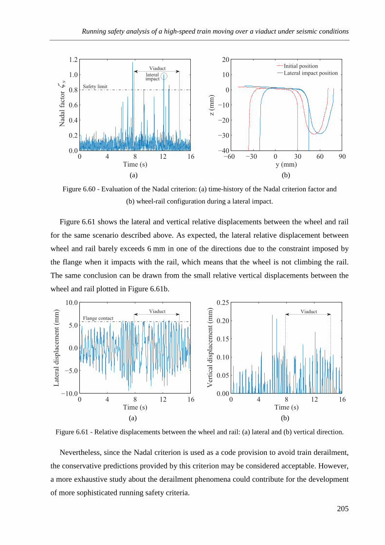
Running safety analysis of a high-speed train moving over a viaduct under seismic conditions
205
(a) (b)
Figure 6.60 - Evaluation of the Nadal criterion: (a) time-history of the Nadal criterion factor and
(b) wheel-rail configuration during a lateral impact.
Figure 6.61 shows the lateral and vertical relative displacements between the wheel and rail
for the same scenario described above. As expected, the lateral relative displacement between
wheel and rail barely exceeds 6 mm in one of the directions due to the constraint imposed by
the flange when it impacts with the rail, which means that the wheel is not climbing the rail.
The same conclusion can be drawn from the small relative vertical displacements between the
wheel and rail plotted in Figure 6.61b.
(a) (b)
Figure 6.61 - Relative displacements between the wheel and rail: (a) lateral and (b) vertical direction.
Nevertheless, since the Nadal criterion is used as a code provision to avoid train derailment,
the conservative predictions provided by this criterion may be considered acceptable. However,
a more exhaustive study about the derailment phenomena could contribute for the development
of more sophisticated running safety criteria.
0 4 8 12 160.0
0.2
0.4
0.6
0.8
1.0
1.2
Time (s)
Nad
al f
acto
rN
ζViaduct
lateral impact
Safety limit
−60 −30 0 30 60 90−40
−30
−20
−10
0
10
20
y (mm)
z (m
m)
Initial position
Lateral impact position
0 4 8 12 16−10.0
−5.0
0.0
5.0
10.0
Time (s)
Lateral displacement (mm) Viaduct
Flange contact
0 4 8 12 160.00
0.05
0.10
0.15
0.20
0.25
Time (s)
Ver
tica
l d
isp
lace
men
t (m
m)
Viaduct

Chapter 6
206
6.8.6.2 Wheel unloading criterion evaluation
The wheel unloading criterion aims to evaluate the risk of derailment in scenarios in which
one of the wheels loses contact with the rail. However, the detachment of one wheel does not
necessarily mean that the train will derail, i.e., the wheel may lose contact with the rail for a
short period of time without compromising the train running safety.
In order to evaluate the degree of conservativeness of this criterion, the time-history of the
wheel unloading criterion factor for the left wheel of the second wheelset obtained in the
scenario described in the previous section, together with the wheel-rail configuration in an
instant in which the wheel detaches from the rail, is plotted in Figure 6.62. Although the
separation between the wheel and rail is notorious, it is not enough to provoke derailment, since
the wheel flange is still far from rising above the rail.
(a)
(b) (c)
Figure 6.62 - Evaluation of the wheel unloading criterion: (a) time-history of the wheel unloading
criterion factor, (b) wheel-rail configuration during detachment and (c) zoom on the tread region.
0 4 8 12 16
−0.6
−0.3
0.0
0.3
0.6
0.9
1.2
1.5
Time (s)
Wheel unloading factor
Uζ Viaduct
detachmentSafety limit
−60 −30 0 30 60−40
−30
−20
−10
0
10
20
x (mm)
y (
mm
)
Initial position
Unloading position
Zoom region
−20 −15 −10 −5 0 5 10−1.5
−1.0
−0.5
0.0
0.5
1.0
1.5
x (mm)
y (
mm
)
Initial position
Unloading position
Wheel
Rail
Rail
Wheel
Intersecion volume
Wheel-rail separation

Running safety analysis of a high-speed train moving over a viaduct under seismic conditions
207
6.8.6.3 Evaluation of the remaining criteria
Regarding the remaining criteria, both of them may also be open to criticism. The
Prud'homme criterion is based on the lateral resistance of a standard track, which may be far
different from the actual track that is being studied. Furthermore, the lateral resistance of the
track may be easily changed by improving the ballast quality or the rail fasteners, leading to an
even more conservative limit value given by the Prud'homme criterion. Similar conclusions
may be drawn regarding the rail roll criterion, since the rotation of the rails is strongly
influenced by the stiffness provided by the rail fasteners. Therefore, the adoption of these two
criteria to evaluate the running stability of a railway vehicle without taking into account the
characteristics of the existing track should be made with some precautions.
6.9 CONCLUDING REMARKS
A study regarding the assessment of the running safety of trains on bridges subjected to
earthquakes is presented. The vehicle-structure interaction method presented in Chapter 4,
which takes into account the geometry of the wheel and rail surfaces and the behavior of the
contact interface in the normal and tangential directions, is adopted to solve the dynamic
problem.
The study focuses on the dynamic analysis of a high-speed train running over an idealized
viaduct based on an existing flyover type structure of the Portuguese railway network situated
in the city of Alverca. This viaduct has been extensively studied by Malveiro et al. (2013), both
numerically and experimentally, thus providing essential data for developing the numerical
model. However, for simplicity of the model, a constant span length of 21 m, based on the most
typical span of the actual structure, and a constant pier height of 10 m are adopted.
The two main sources of excitation of the train-structure system considered in the present
study are the track irregularities and the earthquake action. The irregularities are defined as a
stochastic Gaussian ergodic process and artificially generated based on analytical PSD
functions. Regarding the earthquake action, it is represented in terms of artificial accelerograms
generated from the elastic spectra described in EN 1998-1 (2004), with PGA corresponding to
moderate seismic events with relatively high probability of occurrence and return periods
ranging from 95 to 310 years. This type of seismic actions is of the utmost importance, since
the running safety of the trains might be jeopardized due to the excessive vibrations caused to
the track, even if the structure does not experience significant damage. Therefore, all the

Chapter 6
208
dynamic train-structure interaction analyses are performed in the elastic domain, being the
reduction in the stiffness of the piers due to concrete cracking evaluated by a methodology
specially developed for this purpose. The methodology consists of calibrating the effective
stiffness of the piers in order to obtain, with a linear dynamic analysis, levels of displacement
on the piers similar to those obtained with the nonlinear dynamic analysis. In the present study,
a good agreement is observed between the two responses, proving the efficiency of the
methodology for dealing with moderate earthquakes.
The dynamic responses of both the viaduct and vehicle are analyzed. Since only the lateral
component of the earthquake is considered in the present work, the vertical response of the
deck is not affected by the seismic action. On the other hand, in the lateral direction, the deck
response is mainly dominated by the earthquake, being the influence of the vehicle almost
negligible.
The influence of the effective stiffness of the piers on the lateral response of the viaduct is
also assessed. Two scenarios of seismicity are analyzed with reference return periods of
95 years and 310 years. As would be expected, although the spectral acceleration decreases due
to the increase in the period of the structure, the amplitude of the response increases due to the
fact that the piers become less stiff and therefore may experience larger displacements during
the earthquake.
Regarding the vehicle and its vertical response, the efficiency of the suspensions on filtering
the high frequencies arising from the contact between wheel and rail is perfectly clear when
comparing the accelerations on the wheelset and carbody, especially at high-speeds. The
maximum vertical acceleration at the wheelset increases from 5.4 m/s2 to 17.5 m/s2 for speeds
of 200 km/h and 350 km/h, respectively, while the acceleration at the carbody remains
approximately constant (3.46 m/s2 and 3.65 m/s2 for the minimum and maximum speed
mentioned earlier). It is important to notice that the increase in speed also influences the
vertical contact forces between wheel and rail, since the maximum values obtained for speeds
of 200 km/h and 350 km/h are, respectively, 85 kN and 110 kN, which represents an increase of
about 54 % and 100 % over the static load value of 55 kN of each wheel.
Unlike in the vertical direction, the lateral response of the vehicle is significantly affected by
the earthquake. Under seismic conditions (seismic action with T =310 years), the maximum
lateral displacement of the carbody, relative to the lateral displacement of the track centerline,
is approximately six times higher than the maximum displacement of the wheelset, while

Running safety analysis of a high-speed train moving over a viaduct under seismic conditions
209
without earthquake this difference is almost negligible. In order to avoid excessive lateral
displacement of the carbody during the occurrence of an earthquake, most of the high-speed
trains have stoppers installed in the secondary transversal suspensions. However, for the levels
of seismicity considered in the present work, these devices do not have an important impact in
the lateral response of the vehicle, since the maximum displacements of the carbody with and
without the presence of stoppers do not show considerable differences.
In the last part of the chapter, the influence of the seismic intensity level, running speed and
track quality on the running safety of the railway vehicle moving over the viaduct is discussed.
Unlike the majority of studies in this field, in which the earthquake is assumed to start at the
instant the train enters the bridge, the time offset between the beginning of the earthquake and
the entry of the vehicle in the viaduct is taken into account by considering five scenarios
corresponding to different instants in which the earthquake starts to excite the viaduct. The
consideration of these scenarios is of the utmost importance, since the random nature of the
seismic action, together with the vast number of possible combinations regarding the time
offset between the start of the earthquake and the entry of the vehicle in the viaduct, makes it
almost impossible to find a unique scenario that could be representative of all possible
situations. Thus, as expected, the sensibility analysis carried out in the present chapter proved
that the most critical scenario is not always the same for the different scenarios considered in
this work. Nevertheless, a stochastic approach of the problem would be necessary to obtain a
more representative range of results.
Regarding the running safety analysis, the results show that, even for the moderate seismic
intensities considered in the present study, the train safety is put at risk in a considerable
number of scenarios, thus proving the importance of taking low intensity earthquakes into
account in the design of railway bridges, even if they do not represent a major threat to the
structural integrity. The train running speed is also an important factor to take into account
during the design of railway bridges, especially in regions prone to earthquakes, since all the
safety criteria show that, in the presence of a seismic excitation, the risk of derailment
significantly increases for speeds above 250 km/h. Moreover, the vibrations caused by the
presence of irregularities in poorly maintained tracks may considerably increase the risk of
derailment, even without the presence of earthquakes.
All the information obtained in the dynamic analyses is condensed in the running safety
charts, which consist of the global envelope of each analyzed safety criterion as function of the

Chapter 6
210
running speed of the vehicle and of the seismic intensity level. These charts allow a quick
interpretation of the results, providing a useful tool for analyzing which scenarios may pose a
significant threat to the stability of the vehicle and, consequently, to the safety of the
passengers. As would be expected, the trend observed in all the criteria is similar, indicating
that the risk of derailment increases with the increasing of the running speed and seismic
intensity. It may be observed that the risk of derailment due to the wheel unloading is null when
the train runs over a track whose quality corresponds to the regular operation limit. For this
level of irregularities, the Prud'homme criterion proved to be the most conservative, since it
controls the derailment risk for almost all the speeds. However, this tendency changes for
poorer quality tracks, in which the Nadal, rail roll and wheel unloading criteria define the safety
zone. Hence, for the track with better quality, the vehicle remains safe at every speed if no
earthquake occurs, while for the track with poorer quality, the derailment risk predicted with
the majority of the criteria significantly increases for speeds above 270 km/h.
Finally, the critical analysis regarding the safety criteria adopted in the present work show
that the Nadal criterion is very conservative, even considering that it is only violated if the ratio
between lateral and vertical contact forces exceeds the maximum value for more than 0.015 s,
as proposed by the Japanese standards. Such conclusion becomes clear when looking at the
lateral relative displacement between wheel and rail. These displacements barely exceed 6 mm
in one of the directions due to the constraint imposed by the flange when it impacts with the
rail, which means that the wheel is not climbing the rail. Furthermore, the wheel unloading
criterion proved to be conservative as well, since even when the wheel detaches from the rail,
the wheel flange is still far from rising above the rail.

211
Chapter 7
CONCLUSIONS AND FUTURE DEVELOPMENTS
7.1 CONCLUSIONS
The present thesis is focused on the assessment of the running safety of trains on bridges,
with special emphasis given to the running safety against earthquake. The methodology
proposed to achieve this goal includes the development, implementation, validation and
application of a numerical tool to analyze the dynamic coupling between the train and the
structure.
In Chapter 2, an overview of the recent studies carried out in the field of rail traffic stability
over bridges, with special focus on the running safety against earthquakes, was presented. In
this chapter, a review of the different existing methods for analyzing the dynamic response of
the vehicle-structure system was also made, emphasizing the main advantages and
disadvantages of each one in terms of accuracy and computational cost. Since the majority of
the running safety criteria are related with the control of the wheel-rail contact forces, the
wheel-rail contact model used in the vehicle-structure interaction tool is of the utmost
importance to obtain accurate results. Therefore, the most common wheel-rail contact models
existing in the literature were revisited, together with the recommendations and norms
regarding the stability and safety of trains defined in the standards from different regions of the
world.
Chapter 7
212
As mentioned earlier, the main objective of the present thesis consisted on developing a
methodology for evaluating the running safety of trains moving on bridges. The proposed
methodology was, therefore, described in Chapter 3, in which the risk of derailment is
evaluated using safety criteria based on the wheel-rail contact forces computed in the
train-structure interaction dynamic analysis. The seismic motion applied to the system was
represented in terms of ground acceleration time-histories using artificial accelerograms that
were generated from the elastic spectra described in EN 1998-1 (2004), with PGA
corresponding to moderate events with relatively high probability of occurrence and low return
periods. Since no significant nonlinearity is expected to be exhibited in the bridge piers for
these levels of seismicity, all the analysis were performed in the elastic domain with a reduction
in the stiffness of the piers to account for concrete cracking. This reduced stiffness, referred to
as effective stiffness, was calculated based on a simplified methodology that proved to be
efficient for dealing with moderate earthquakes.
Another important source of excitation that was also included in the methodology consisted
in the track irregularities. These deviations of the rail from the ideal geometry were artificially
generated, based on a stationary stochastic process described by PSD functions.
According to the proposed methodology, for each analyzed scenario, the circulation is
considered to be safe as long as none of the adopted safety criteria used to assess the train
running safety is violated during the whole time that the vehicle is crossing the bridge.
The train-structure interaction method developed in the present thesis was formulated in
Chapter 4 and validated in Chapter 5. The tool was implemented in MATLAB, being the
structural models of both the vehicle and bridge developed in the finite element software
ANSYS. The structural matrices are imported by MATLAB from ANSYS using an efficient
interconnection tool between both softwares. The main feature of the method consists in a
wheel-rail contact model that takes into account the geometry of the wheel and rail surfaces in
order to accurately evaluate the lateral interaction. This contact model is divided in three main
parts, namely the geometric problem, the normal problem and the tangential problem.
The geometric problem, which consists of detecting the position of the contact points
between wheel and rail, is solved online. Although this procedure is computationally more
expensive than an offline contact approach, in which the location of the contact points is
precalculated as a function of the relative displacements between wheel and rail, its higher
accuracy outweighs this drawback. The proposed method is able to look for potential contact

Conclusions and future developments
213
points in any types of geometrical surfaces (convex or concave) at both the tread and the flange
of the wheel. Thus, the formulation is suitable to investigate not only scenarios related to
ordinary railway operation, but also derailment situations, in which the flange contact plays an
important role.
Regarding the normal contact problem, the nonlinear Hertz theory was used to compute the
normal contact forces between wheel and rail. Although this theory rests on a series of
assumptions that may limit its range of application, it offered a good compromise between
computational efficiency and accuracy for dealing with the dynamic analysis of railway
vehicles.
For simulating the behavior at the contact interface in the tangential direction, three different
approaches were adopted. Since the exact theory of rolling contact proposed by Kalker is
impracticable to be used in dynamic analysis of railway vehicles due to its excessive
computational cost, the Polach method, the Kalker's book of tables and the Kalker's linear
theory were implemented and integrated in the proposed formulation. The first two methods
combine accuracy with computational efficiency, while the latter is limited to scenarios with
small creepages.
The coupling between the vehicle and the structure was accomplished by the direct method,
which complements the governing equilibrium equations of the vehicle and structure with
additional constraint equations that relate the displacements of the contact nodes of the vehicle
with the corresponding nodal displacements of the structure. These equations form a single
system, with displacements and contact forces as unknowns, that is solved directly using an
optimized block factorization algorithm.
The train-structure interaction method mentioned above was validated with three numerical
applications and one experimental test described in Chapter 5. The first application consisted of
validating the creep models implemented and integrated in the numerical tool. Four test cases
based on examples presented in Kalker (1990), in which the longitudinal and lateral creep
forces are computed for distinct ranges of creepages and semi-axes ratios of the contact ellipse,
were reproduced. All the three creep models proved to be adequate to deal with scenarios with
small creepages. However, the Kalker's linear model could not predict reasonable values of the
creep forces when the creepages increase and the tangential stresses approach the saturation
limit. For higher values of translational creepages and low values of spin, both the Polach
method and the Kalker's book of tables provided adequate results, but only the latter was

Chapter 7
214
sufficiently accurate for situations where the spin creepages were also higher. For these
reasons, the implemented book of tables was used in the majority of the dynamic simulations
presented in this thesis.
In the second application, the Manchester Benchmark was revisited. The benchmark
comprised a series of tests that consisted of prescribing, both statically and dynamically, lateral
displacements and yaw rotations to a single wheelset in order to analyze its behavior. Several
contact characteristics were analyzed, namely the contact point positions on both wheels of the
wheelset, the rolling radius difference between wheels, the contact angles and the creepages.
The results obtained with the proposed method for all the analyzed quantities showed an
excellent agreement with those obtained with widely used softwares in railway vehicle
dynamics, such as GENSYS, NUCARS and VAMPIRE.
The third numerical example consisted of evaluating the lateral stability of a single wheelset
running at several speeds. The dynamic response of the wheelset calculated with the proposed
method was compared with that obtained using a semi-analytical model with two degrees of
freedom available in the literature. The model follows a number of simplifying assumptions
whereby the dynamics of the wheelset could be described by simple linear differential
equations. A good agreement between the responses obtained with the proposed method and
those obtained by the integration of the equations of motion of the semi-analytical model was
observed. As expected, for speeds below the critical limit, both the lateral displacement and the
yaw rotation of the wheelset tended to damp out after being driven away by a lateral
disturbance. This was due to the energy dissipation provided by the creep forces and to the
stability provided by the suspensions. However, when the speed exceeded the critical value, the
behavior of the wheelset became unstable, leading to a hunting motion that grew indefinitely.
In the last application, an experimental test conducted in the rolling stock test plant of the
RTRI in Japan, in which a full scale railway vehicle ran over a track that was subjected to
vertical and lateral deviations, was reproduced numerically. The lateral accelerations inside the
carbody measured during the test were compared with those obtained with the proposed
method and with the train-structure interaction software DIASTARS. The results showed a
good agreement, even during extreme situations, such as flange-rail impacts due to excessive
lateral vibrations cased by the rail deviations. Some discrepancies, however, were observed
between the numerical and experimental results. These may be caused by the fact that vehicle
was modeled using rigid bars and thus important deformations were not considered.
Conclusions and future developments
215
Furthermore, the incapacity of the actuators to reproduce with precision the track rotations
could also contribute for the differences between the experimental and numerical results.
In summary, the results obtained in the four validation applications showed that the
implemented tool is sufficiently accurate to deal with a vast range of scenarios regarding the
running safety of trains moving on bridges.
Finally, in Chapter 6, a study regarding the assessment of the running safety of a train
moving on a viaduct subjected to earthquakes was carried out. The dynamic analyses were
performed with the vehicle-structure interaction method presented in Chapter 4 and validated in
Chapter 5.
The study focused on the dynamic analysis of a high-speed train running over an idealized
viaduct based on an existing flyover type structure of the Portuguese railway network. This
viaduct has been extensively studied in the past, both numerically and experimentally, thus
providing essential data for developing the numerical model.
The two main sources of excitation of the train-structure system considered in the study
were the track irregularities and the earthquake load, which were described in Chapter 3. Since
the seismic excitation was not expected to cause significant damage to the structure, all the
dynamic train-structure interaction analyses were performed in the elastic domain, being the
reduction in the stiffness of the piers due to concrete cracking evaluated using the methodology
exposed in Chapter 3. As mentioned before, the methodology consisted of calibrating the
effective stiffness of the piers in order to obtain, with a linear dynamic analysis, levels of
displacement on the piers similar to those obtained with the nonlinear dynamic analysis. In the
present study, a good agreement was observed between the two responses, proving the
efficiency of the methodology.
Before starting the running safety analysis, a preliminary study for evaluating the dynamic
behavior of the train-structure system was carried out. As a first conclusion, the vertical
response of both the structure and the vehicle was barely affected by the seismic action, since
only the lateral component of the earthquake was considered in the present work. On the other
hand, in the lateral direction, the deck response was mainly dominated by the earthquake, being
the influence of the vehicle load almost negligible.
The influence of the effective stiffness of the piers on the lateral response of the viaduct was
also assessed. Two scenarios of seismicity were analyzed with reference return periods of

Chapter 7
216
95 years and 310 years. Although the spectral acceleration decreased due to the increase in the
period of the structure, the amplitude of the response increased due to the fact that the piers
became less stiff and therefore could experience larger displacements during the earthquake.
Regarding the vehicle, when the viaduct was subjected to the strongest earthquake
considered in this study, the maximum lateral displacement of the carbody, relative to the
lateral displacement of the track centerline, was approximately six times higher than the
maximum displacement of the wheelset, while without earthquake this difference was almost
negligible. In order to avoid excessive lateral vibrations, the high-speed trains are equipped
with stoppers installed in the secondary lateral suspensions. However, it was concluded that for
the levels of seismicity considered in the present work, these devices do not have an important
impact in the lateral response of the vehicle.
Finally, the influence of the seismic intensity level, running speed and track quality on the
running safety of the railway vehicle was discussed. Unlike the majority of studies, in which
the earthquake is assumed to start at the instant the train enters the bridge, a time offset between
the beginning of the earthquake and the entry of the vehicle in the viaduct was taken into
account by considering five scenarios corresponding to different instants in which the
earthquake starts to excite the viaduct. The adoption of these scenarios proved to be of the
utmost importance, since the results obtained in the sensibility analysis carried out in this
chapter showed that the most critical scenario for the train's running safety was not always the
same for the different situations considered in the study. This conclusion was expected, since it
is very difficult to find a unique scenario that could be representative of all possible cases.
The running safety analysis showed that even for the moderate seismic intensities
considered in the present study, the train safety was put at risk in a considerable number of
scenarios, thus proving the importance of taking low intensity earthquakes into account in the
design of railway bridges, even if they do not represent a major threat to the structural integrity.
The train running speed is also an important factor to take into account during the design of
railway bridges, especially in regions prone to earthquakes, since all the safety criteria showed
that, in the presence of a seismic excitation, the risk of derailment significantly increased for
speeds above 250 km/h. Moreover, the vibrations caused by the presence of irregularities in
poorly maintained tracks may considerably increase the risk of derailment, even without the
presence of earthquakes.

Conclusions and future developments
217
All the information obtained in the dynamic analyses was condensed in the running safety
charts, which consist in the global envelope of each analyzed safety criterion as function of the
running speed of the vehicle and seismic intensity level. These charts allow a quick
interpretation of the results, providing a useful tool for analyzing which scenarios may pose a
significant threat to the stability of the vehicle and, consequently, to the safety of the
passengers. The trend observed in all the criteria was similar, indicating that the risk of
derailment increases with the increasing of the running speed and seismic intensity. It could be
observed that the risk of derailment due to the wheel unloading was null when the train ran
over a track whose quality corresponded to the regular operation limit. For this level of
irregularities, the Prud'homme criterion proved to be the most conservative, since it controls the
derailment risk for almost all the speeds. However, this tendency changed for poorer quality
tracks, in which the Nadal, rail roll and wheel unloading criteria defined the safety zone.
Hence, for the track with better quality, the vehicle remained safe at every speed when no
earthquake was considered, while for the track with poorer quality, the derailment risk
predicted with the majority of the criteria significantly increased for speeds above 270 km/h.
Finally, the critical analysis regarding the safety criteria adopted in the present work shown
that the Nadal criterion is very conservative, even considering that it is only violated if the ratio
between lateral and vertical contact forces exceeds the limit value for more than 0.015 s, as
proposed by the Japanese standards. The results showed that in the instants in which the limit
value of the criterion was exceeded, the relative lateral displacement between the wheel and the
rail barely exceeded 6 mm due to the constraint imposed by the wheel flange, showing that the
wheel was not climbing the rail as the criterion intended to prove.
7.2 FUTURE DEVELOPMENTS
The work presented in this thesis focuses on developing a methodology for the assessment
of the train running safety on bridges, including a train-structure interaction tool fully
developed by the author. However, the course of this research raised several questions that
were not addressed. In this context, some topics requiring further analysis are referred in the
following paragraphs:
a) The train-structure interaction tool developed in this thesis still requires further work,
especially regarding the computational efficiency. The use of direct integration to solve
the dynamic equations of motion of the train-structure system represents a significant

Chapter 7
218
fraction of the total time needed to solve the whole dynamic problem. The
implementation of the modal superposition method could be an important step towards a
better computational efficiency in linear problems. Moreover, it would be interesting to
exploit the potential of the parallel computation provided by the Graphic Processing
Unit (GPU) toolbox of MATLAB. Although there are still no functions in this toolbox
to solve system of equations defined by sparse matrices, this could be an important
improvement in the near future;
b) Still regarding the interaction tool, further work is needed in the wheel-rail contact
model developed in this thesis. A better computational efficiency is necessary in the
geometric contact problem, especially on the algorithm used to locate the contact points
in concave regions. This is an important drawback in analysis with worn profiles, where
the concave region that exists in the transition between the tread and flange plays an
important role. Moreover, the time needed to locate the contact points in each wheel is
still an important limitation in the analysis of long trains with a large number of cars;
c) The implementation of more realistic models to deal with the normal contact problem
may also be an important development in the future. Although the Hertz theory offers a
good compromise between computational efficiency and accuracy in the dynamic
analysis of railway vehicles, a more realistic model would be needed to deal with local
problems such as wear;
d) It is intended to extend the formulation to deal with curve tracks. Although the
high-speed railway recommendations impose restrictions on the curve radii, the curve
negotiation is a topic of the utmost importance in railway engineering, since it is one of
the major causes of derailments. To accomplish this goal, the wheel-rail contact model
requires some improvements, since, in the two-point contact scenario, the contact point
search is no longer restricted to only one plane;
e) In the present work, only moderate earthquakes that do not represent a major threat to
the structural integrity were studied. However, the evaluation of the running safety of
trains under stronger seismic conditions is a topic to be addressed in the future. To
achieve that, the structure model has to account for the effects of both the material
inelasticity and the geometric nonlinearity due to the large displacements caused by the
earthquake;

Conclusions and future developments
219
f) The analysis of the influence of the vertical ground motion on the running safety of
trains moving on bridges is also an important topic to be addressed in the future.
Although the majority of the authors reported that the vehicle running safety against
earthquake has a stronger relation to the lateral ground motions than to the vertical
excitations, the inclusion of the vertical ground motion might contribute to a better
understanding of some of the derailment mechanisms presented in this thesis;
g) The case study presented in this thesis focuses on the running safety analysis of a
railway vehicle running over a simply supported multi-span viaduct based on an existent
viaduct belonging to the Portuguese railway network. However, a wider parametric
study, comprehending different types of viaducts and bridges (different support
conditions, pier heights and structural solutions), different types of trains and more
types of earthquake (different soil conditions and seismic zones), might contribute to a
more representative conclusion;
h) It is intended to evaluate in the future the running safety of trains moving over bridges
under other types of actions, such as crosswinds. Although the methodology proposed
in the present thesis allows this type of analysis, only the running safety against
earthquakes is addressed in the case study;
i) It may be necessary in the future a stochastic approach to deal with the type of problems
discussed in this work, since there is a vast number of uncertainties presented. For
example, the random nature of the seismic action, together with the vast number of
possible combinations regarding the time offset between the start of the earthquake and
the entry of the vehicle in the viaduct, makes it difficult to obtain representative results
exclusively with a deterministic approach.
j) The running safety criteria adopted in the present work are, in most cases, very
conservative. In fact, some experimental tests referred in Chapter 2 reported that a train
might be far from derail if the criteria limits are exceeded only for a short period of
time. Moreover, the critical analysis performed at the end of Chapter 6 led to similar
conclusions. Therefore, a better understanding of the physical meaning of the
derailment phenomena may contribute for the development of more sophisticated
running safety criteria.
k) It would be interesting to integrate the numerical tool proposed in the present thesis in a
railway monitoring system used to evaluate the necessity of maintenance. With such

Chapter 7
220
kind of monitoring system, it would be possible to avoid the huge periodic maintenance
operations, contributing to a more optimized maintenance program.

221
Appendix A
IMPLEMENTATION OF A CONTACT LOOKUP TABLE
A.1 INTRODUCTION
For computing the contact lookup table, the track and wheelset are assumed to be rigid. The
relative motion between them occurs in a plane perpendicular to the track, being the wheelset
allowed to rotate about the track longitudinal axis (roll rotation). Furthermore, the contact
between the wheel and rail occurs at only one point and no separation is allowed. Under these
assumptions, the surface parameters rs and ws (see Section 4.3.1 of Chapter 4) can be
computed as a function of the relative lateral displacement wy between the wheelset and track.
A.2 COORDINATE SYSTEMS
For the computation of the contact lookup tables and assuming that the wheelset is rigid, two
new coordinate systems have to be introduced, namely the track centerline and the wheelset
coordinate systems (see Figure A.1).
The track centerline coordinate system ( )tctctc zyx ,, has its origin at a point equidistant from
the two rails that is located at the same height as the point where the wheel contacts the rail
when the wheelset is centered with the track. The tcx axis is orientated tangent to the track
centerline, while the tcy and tcz are contained in the rail cross-section plane orientated,

Appendix A
222
respectively, parallel and perpendicular to the rail-bed horizontal plane. Since the track
rotations are not considered in the contact table computation, the axes that form the track
centerline coordinate system are parallel to those which form the target element and the rail
profile coordinate systems.
The wheelset coordinate system ( )wswsws zyx ,, is fixed with the wheelset and has its origin
at the center of mass of the wheelset. The wsy and wsz are contained in the wheelset
cross-section plane, being the former orientated along the wheelset axis. The transformation
matrix from the track centerline coordinate system to the wheelset coordinate system is
analogous to the matrix twT defined in equation (4.8), since the wheelset behaves as a rigid
body and the track rotations are not considered.
Figure A.1 - Track centerline and wheelset coordinate systems.
A.3 PARAMETERIZATION OF THE RAIL AND WHEEL PROFILES
A.3.1 Parameterization of the rail profile
The two-dimensional surface geometry of the rail is parameterized with respect to the
centerline coordinate system and described in terms of the surface parameter rs , as depicted in
Figure A.2.
L L
tcy
tcz
tcx
wsz
wsy

Implementation of a contact lookup table
223
Figure A.2 - Parameterization of the rail profile with respect to the track centerline coordinate system.
The position vector tcRu of an arbitrary point R of the rail surface, defined with respect to the
track centerline coordinate system, is given by
rR
tc
rOtcR uuu += (A.1)
where rRu is defined in equation (4.10) and tc
rOu is the position vector of the origin of the rail
profile coordinate system, defined with respect to the track centerline coordinate system,
written as
[ ]T00 Ltc
rO ±=u (A.2)
where L is the distance along the tcy axis between the origins of the track centerline and rail
profile coordinate systems (the sign depends whether the left or right wheel is being analyzed).
A.3.2 Parameterization of the wheel profile
Assuming that the wheel belongs to a rigid wheelset, its profile is parameterized with respect
to the centerline coordinate system and described in terms of the surface parameter ws , as
shown in Figure A.3.
L
( )r rf s
rs
tcy
tcz
tcxr
y
rz
R
rOr
Rutc
Ru
r
tc
Ou

Appendix A
224
Figure A.3 - Parameterization of the wheel profile belonging to a rigid wheelset with respect to the track
centerline coordinate system.
The position vector tcWu of an arbitrary point W of the wheel surface, defined with respect to
the track centerline coordinate system, is given by
( )wW
ws
wO
Ttwtc
wsOtcW uuTuu ++= (A.3)
where wWu is defined in equation (4.16) of Chapter 4, tc
wsOu is the position vector of the origin of
the wheelset coordinate system, defined with respect to track centerline coordinate system,
expressed as
( )[ ]T
00 tcw
tcw
tc
wsO zRy +=u (A.4)
where tcwy and tc
wz are, respectively, the lateral and vertical displacements of the center of mass
of the wheelset, defined with respect to the track centerline coordinate system, and 0R the
initial rolling radius of the wheel. The position vector of the origin of the wheel profile
coordinate system ws
wOu , defined with respect to the wheelset coordinate system, is given by
[ ]T00 RLws
wO −±=u (A.5)
wheelset
axis
L
tcy
tcz
tcx
0R
wsz
wsy
ws
( )w wf swy
wz
wO
w
Wu tc
Wu
w
ws
Ouws
tc
Ou
wsO
L
rO

Implementation of a contact lookup table
225
A.4 CONTACT POINT SEARCH AND TABLE STORAGE
Since the accuracy of the contact table depends on the degree of discretization used, the
wheel and rail surfaces are discretized by a set of points that reliably represent the profile
geometry. Hence, for a given lateral displacement of the wheelset, the vertical distances
between each point of the wheel and rail surfaces are evaluated, as shown in Figure A.4. Using
this set of vertical distances, the points with maximum absolute value, which belong to the
intersection between the wheel and rail surfaces, are considered to be potential contact points.
Since the wheelset is rigid, the potential contact points are in contact only if the following
condition is met:
ε<∆−∆ rhtlft zz maxmax (A.6)
where maxz∆ is the maximum vertical distance between the wheel and rail in the region where
the surfaces intersect each other, and ε is a specified tolerance. The superscripts lft and rht
indicate left and right side of the wheelset, respectively. For each side, the distance maxz∆ is
given by
( ) wtcztc
iwtc
iw niz ,,2,1,max ,,max …=⋅−=∆ euu (A.7)
where nw is the number of points that discretize the wheel surface, tcze is a unit base vector of
the track centerline coordinate system, tciw,u is defined by equation (A.3) and tciw,u is the position
vector of the vertical projection of the ith wheel point into the rail surface, defined with respect
to the track centerline coordinate system, as depicted in Figure A.4. Note that the calculation of
the vertical distances iz∆ could also be performed, in an analogous way, using the points of the
rail surface.
Figure A.4 - Vertical distances between wheel and rail (intersection scale exaggerated).
wf
rf
iz∆maxz∆tc
y
tcz
tcxtc
w,iui
,
tc
w iu

Appendix A
226
If the condition (A.6) is not fulfilled, the wheelset roll rotation tcwφ , defined with respect to
the track centerline coordinate system, has to be iteratively adjusted. According to Li (2002),
the number of iterations can be substantially reduced if the roll rotation of the wheelset is
adjusted by an angle tcwφ∆ given by
( )tcy
rhttcw
lfttcw
rhtlfttcw
zz
euu ⋅−∆−∆=∆,max,
,max,
maxmaxφ (A.8)
where tcw max,u is the position vector of the point of the wheel with maximum vertical distance to
the rail in the region where the surfaces intersect each other, with respect to the track centerline
coordinate system, and tcye is a unit base vector of the track centerline coordinate system. The
contact search is repeated until the tolerance specified in the condition (A.6) is satisfied, being
the surface parameters that define the contact point position in each wheel of the wheelset
stored in the contact table.
The vertical displacements of the center of mass of the wheelset tcwz and the wheelset roll
rotation tcwφ , the contact angles on both wheels γ and the surface parameters sr and sw, defined
as a function of the lateral displacement of the center of mass of the wheelset tcwy , are plotted in
Figures A.5 to A.7. These results refer to the S1002 wheel and UIC60 rail.
(a) (b)
Figure A.5 - Wheelset movement as a function of the relative lateral displacement between wheelset and
rail: (a) vertical displacements and (b) roll rotations.
−20 −15 −10 −5 0 5 10 15 200.0
2.5
5.0
7.5
10.0
12.5
15.0
( )mmtc
wy
()
mm
tc wz
−20 −15 −10 −5 0 5 10 15 20−20
−15
−10
−5
0
5
10
15
20
( )mmtc
wy
()
mrad
tc wφ

Implementation of a contact lookup table
227
Figure A.6 - Contact angles as a function of the relative lateral displacement between wheelset and rail.
(a) (b)
Figure A.7 - Surface parameters as a function of the relative lateral displacement between wheelset and
rail: (a) rail parameter and (b) wheel parameter.
−20 −15 −10 −5 0 5 10 15 20−80
−60
−40
−20
0
20
40
60
80
(º
)
Left wheel
Right wheel
( )mmtc
wy
γ
−20 −15 −10 −5 0 5 10 15 20−40
−30
−20
−10
0
10
20
30
40
s r (m
m)
Left rail
Right rail
( )mmtc
wy
−20 −15 −10 −5 0 5 10 15 20−60
−45
−30
−15
0
15
30
45
60
yw
(mm)
s w (
mm
)Left wheel
Right wheel


229
Appendix B
COEFFICIENTS FOR THE NORMAL AND TANGENTIAL
CONTACT PROBLEMS
B.1 INTRODUCTION
This appendix aims to summarize the coefficients needed for solving the normal and
tangential contact problems described in Sections 4.4 and 4.5, respectively, of Chapter 4. These
are:
a) Hertz coefficients m and n for computing the semi-axes of the contact ellipse;
b) Hertz constant Ch for computing the generalized stiffness coefficient;
c) Kalker's creepage coefficients cij.
B.2 HERTZ COEFFICIENTS FOR COMPUTING THE SEMI-AXES OF T HE
CONTACT ELLIPSE
The Hertz coefficients m and n used to compute the semi-axes of the contact ellipse (see
equation (4.37)) are given as a function of the angular parameter θ defined in equation (4.38).
These coefficients are summarized in Table B.1 for values of θ ranging from 0 to 180 degrees.
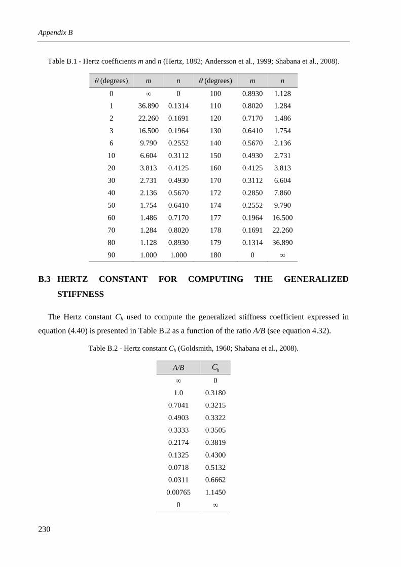
Appendix B
230
Table B.1 - Hertz coefficients m and n (Hertz, 1882; Andersson et al., 1999; Shabana et al., 2008).
θ (degrees) m n θ (degrees) m n
0 ∞ 0 100 0.8930 1.128
1 36.890 0.1314 110 0.8020 1.284
2 22.260 0.1691 120 0.7170 1.486
3 16.500 0.1964 130 0.6410 1.754
6 9.790 0.2552 140 0.5670 2.136
10 6.604 0.3112 150 0.4930 2.731
20 3.813 0.4125 160 0.4125 3.813
30 2.731 0.4930 170 0.3112 6.604
40 2.136 0.5670 172 0.2850 7.860
50 1.754 0.6410 174 0.2552 9.790
60 1.486 0.7170 177 0.1964 16.500
70 1.284 0.8020 178 0.1691 22.260
80 1.128 0.8930 179 0.1314 36.890
90 1.000 1.000 180 0 ∞
B.3 HERTZ CONSTANT FOR COMPUTING THE GENERALIZED
STIFFNESS
The Hertz constant Ch used to compute the generalized stiffness coefficient expressed in
equation (4.40) is presented in Table B.2 as a function of the ratio A/B (see equation 4.32).
Table B.2 - Hertz constant Ch (Goldsmith, 1960; Shabana et al., 2008).
A/B hC
∞ 0
1.0 0.3180
0.7041 0.3215
0.4903 0.3322
0.3333 0.3505
0.2174 0.3819
0.1325 0.4300
0.0718 0.5132
0.0311 0.6662
0.00765 1.1450
0 ∞

Coefficients for the normal and tangential contact problems
231
B.4 KALKER'S CREEPAGE COEFFICIENTS
The Kalker's creepage coefficients cij depend on the semi-axes ratio a/b (see equation (4.37))
and on the Poisson's ratio of the wheel and rail materials ν. Table B.3 summarizes these
coefficients, including closed-form expressions to compute their values for high and low
semi-axes ratios.
Table B.3a - Kalker's creepage coefficients cij for b > a (Garg and Dukkipati, 1984; Kalker, 1990).
a/b c11 c22 c23= -c32 c33
ν = 0 0.25 0.5 ν = 0 0.25 0.5 ν = 0 0.25 0.5 ν = 0 0.25 0.5
0 Equation (B.1) Equation (B.2) Equation (B.3) Equation (B.4)
0.1 2.51 3.31 4.85 2.51 2.52 2.53 0.33 0.47 0.73 6.42 8.28 11.7
0.2 2.59 3.37 4.81 2.59 2.63 2.66 0.48 0.60 0.81 3.46 4.27 5.66
0.3 2.68 3.44 4.80 2.68 2.75 2.81 0.61 0.72 0.89 2.49 2.96 3.72
0.4 2.78 3.53 4.82 2.78 2.88 2.98 0.72 0.82 0.98 2.02 2.32 2.77
0.5 2.88 3.62 4.83 2.88 3.01 3.14 0.83 0.93 1.07 1.74 1.93 2.22
0.6 2.98 3.72 4.91 2.98 3.14 3.31 0.93 1.03 1.18 1.56 1.68 1.86
0.7 3.09 3.81 4.97 3.09 3.28 3.48 1.03 1.14 1.29 1.43 1.50 1.60
0.8 3.19 3.91 5.05 3.19 3.41 3.65 1.13 1.15 1.40 1.34 1.37 1.42
0.9 3.29 4.01 5.12 3.29 3.54 3.82 1.23 1.36 1.51 1.27 1.27 1.27
Table B.3b - Kalker's creepage coefficients cij for a > b (Garg and Dukkipati, 1984; Kalker, 1990).
b/a c11 c22 c23= -c32 c33
ν = 0 0.25 0.5 ν = 0 0.25 0.5 ν = 0 0.25 0.5 ν = 0 0.25 0.5
1.0 3.40 4.12 5.20 3.40 3.67 3.98 1.33 1.47 1.63 1.21 1.19 1.63
0.9 3.51 4.22 5.30 3.51 3.81 4.16 1.44 1.59 1.77 1.16 1.11 1.06
0.8 3.65 4.36 5.42 3.65 3.99 4.39 1.58 1.75 1.94 1.10 1.04 0.95
0.7 3.82 4.54 5.58 3.82 4.21 4.67 1.76 1.95 2.18 1.05 0.97 0.85
0.6 4.06 4.78 5.80 4.06 4.50 5.04 2.01 2.23 2.50 1.01 0.89 0.75
0.5 4.37 5.10 6.11 4.37 4.90 5.56 2.35 2.62 2.96 0.96 0.82 0.65
0.4 4.84 5.57 6.57 4.84 5.48 6.31 2.88 3.24 3.70 0.91 0.75 0.55
0.3 5.57 6.34 7.34 5.57 6.40 7.51 3.79 4.32 5.01 0.87 0.67 0.45
0.2 6.96 7.78 8.82 6.96 8.14 9.79 5.72 6.63 7.89 0.83 0.60 0.34
0.1 10.7 11.7 12.9 10.7 12.8 16.0 12.2 14.6 18.0 0.80 0.53 0.23
0 Equation (B.6) Equation (B.7) Equation (B.8) Equation (B.9)

Appendix B
232
The cij coefficients for low values of the a/b ratio (see Table B.3a) are given by
( )νπ
−=
14
2
11c (B.1)
4
2
22
π=c (B.2)
( )
−+Λ+−
= ↓ 54ln2
11
1323 νν
π bac (B.3)
( ) ( )bac
νπ
−=
116
2
33 (B.4)
where ↓Λ is given by
( )
=Λ↓ 2
16ln
ba (B.5)
The cij coefficients for high values of the a/b ratio (see Table B.3b) are given by
( ) ( )
−Λ−+
−Λ=
↑↑ ννπ
2
4ln31
2
211
abc (B.6)
( )[ ] ( )
( ) ( )( )
+Λ−−−+
+Λ−=
↑↑νν
ν
νν
π21
4ln311
21
222
abc (B.7)
( ) ( ) νν
π421
1
3
223 +−Λ−
=↑abab
c (B.8)
( )
( )
+−Λ−−Λ
−=↑
↑
νννπ
421
21
433c (B.9)
where ↑Λ is given by
( )
=Λ↑ 2
16ln
ab (B.10)

233
Appendix C
BLOCK FACTORIZATION SOLVER
C.1 INTRODUCTION
The present block factorization algorithm is based on that developed by Neves et al. (2012)
and later extended by Montenegro et al. (2015b) to deal with the three-dimensional contact.
This algorithm aims to solve the system of equations (4.102) efficiently by taking into account
the specific properties of each block, namely symmetry, positive definiteness and bandwidth.
C.2 SOLVER FORMULATION
Since the submatrix YYK presented in equation (4.102) may be indefinite and therefore may
not have a stable factorization without pivoting, the lines and columns of the system matrix
corresponding to the incremental displacements Ya∆ and contact forces X∆ have to be
grouped together. Hence the block factorization of the system of equations (3.101) is presented
below using the following notation.
=
3
2
1
3
2
1
333231
322221
312111
b
b
b
x
x
x
AAA
AAA
AAAT
TT
(C.1)
where 1x and 2x correspond to Ia∆ and Ra∆ , respectively, and 3x corresponds to the group

Appendix C
234
formed by Ya∆ and X∆ . The coefficient matrix presented in equation (C.1) admits the
following factorization
×
=
33
3222
312111
333231
2221
11
333231
322221
312111
U00
LL0
LLL
LLL
0LL
00L
AAA
AAA
AAATT
TTT
T
TT
(C.2)
where L and U are lower and upper triangular matrices, respectively. For simplicity, the
permutation matrices associated with the factorization of 33A are not represented. The block
factorization solver is divided into three stages, which are described below.
By equating part of the corresponding blocks in equation (C.2) the following relations are
obtained
T111111 LLA = (C.3)
TT211121 LLA = (C.4)
The first stage consists of factorizing 11A , which is assumed to be symmetric positive
definite and therefore admits a Cholesky factorization (Burden and Faires, 1997), and
calculating 21L by forward substitution as follows. Since 11A and T21A are time-independent,
the operations associated with equations (C.3) and (C.4) have to be performed only once at the
beginning of the analysis.
By equating the remaining blocks in equation (C.2) the following relations are obtained
TT311131 LLA = (C.5)
T222222 LLA = (C.6)
TTT3222312132 LLLLA += (C.7)
333333 ULA = (C.8)
where
T21212222 LLAA −= (C.9)
TT323231313333 LLLLAA −−= (C.10)
The second stage consists of obtaining the remaining matrices of the right hand side of
equation (C.2) in an analogous way. It is assumed that the matrix 22A admits a Cholesky

Block factorization solver
235
factorization, whereas the submatrices 33L and 33U are obtained using an LU factorization with
pivoting. Since the matrices involved in equations (C.5) to (C.8) depend on the time and
contact conditions, the operations belonging to the second stage have to be performed in each
Newton iteration.
Finally, the third stage of the block factorization algorithm consists of obtaining the solution
of the system of equations through the following two steps.
=
3
2
1
3
2
1
333231
2221
11
b
b
b
y
y
y
LLL
0LL
00L
(C.11)
=
3
2
1
3
2
1
33
3222
312111
y
y
y
x
x
x
U00
LL0
LLLTT
TTT
(C.12)
The vectors1y to 3y are obtained by forward substitution as following
1111 byL = (C.13)
1212222 yLbyL −= (C.14)
2321313333 yLyLbyL −−= (C.15)
being the solution of the system of equations (C.1) obtained by back substitution
3333 yxU = (C.16)
3322222 xLyxL TT −= (C.17)
3312211111 xLxLyxL TTT −−= (C.18)


237
REFERENCES
A
AAR. M1001: Manual of standards and recommended practices: Section C, Part II - Design,
Fabrication, and Construction of Freight Cars, Association of American Railroads, Washington, DC,
USA, 2011.
ABAQUS. Release 6.10, Dassault Systèmes S.A., Paris, France, 2010.
Alexander, N.A. Multi-support excitation of single span bridges, using real seismic ground motion
recorded at the SMART-1 array, Computers & Structures, 2008, 86 (1-2), pp. 88-103.
DOI:10.1016/j.compstruc.2007.05.035.
Allemang, R.J. The Modal Assurance Criterion (MAC): Twenty tears of use and abuse Sound and
Vibration, 2003, 37 (8), pp. 14-21.
Andersson, E., Berg, M., Stichel, S. Rail vehicle dynamics: Fundamentals and guidelines, Royal
Institute of Technology, Stockholm, Sweden, 1999.
ANSYS. Academic Research, Release 13.0, ANSYS Inc., Canonsburg, PA, USA, 2010.
References
238
Antolín, P. Efectos dinámicos laterales en vehículos y puentes ferroviarios sometidos a la acción de
vientos transversales, PhD Thesis, Universidad Politécnica de Madrid, Madrid, Spain, 2013 [in
Spanish].
Antolín, P., Goicolea, J.M., Oliva, J., Astiz, M.A. Nonlinear train-bridge lateral interaction using a
simplified wheel-rail contact method within a finite element framework, Journal of Computational and
Nonlinear Dynamics, 2012, 7 (4), pp. 041014(1) - 041014(9). DOI:10.1115/1.4006736.
Ashford, S.A., Kawamata, Y. Performance of transportation systems during the 2004 Niigata Ken
Chuetsu, Japan, Earthquake, Earthquake Spectra, 2006, 22 (1), pp. 111-132. DOI:10.1193/1.2172282.
Ayasse, J.B., Chollet, H. Determination of the wheel rail contact patch in semi-Hertzian conditions,
Vehicle System Dynamics, 2005, 43 (3), pp. 161-172. DOI:10.1080/00423110412331327193.
Ayasse, J.B., Chollet, H., Maupu, J.L. Paramètres caractéristiques du contact roue-rail (Rapport
INRETS 225), INRETS, Paris, France, 2000.
B
Baker, C., Cheli, F., Orellano, A., Paradot, N., Proppe, C., Rocchi, D. Cross-wind effects on road and
rail vehicles, Vehicle System Dynamics, 2009, 47 (8), pp. 983-1022.
DOI:10.1080/00423110903078794.
Barron de Angoiti, I. High speed rail: Development around the world, In R. Calçada, R. Delgado, A.
Carvalho & G. Degrande (Ed), Workshop Noise and Vibration on High-Speed Railways, Porto,
Portugal, 2008.
Bathe, K.J. Finite element procedures, Prentice-Hall, Upper Saddle River, NJ, USA, 1996.
Bozzone, E., Pennestrì, P., Salvini, P. Dynamic analysis of a bogie for hunting detection through a
simplified wheel–rail contact model, Multibody System Dynamics, 2011, 25 (4), pp. 429-460.
DOI:10.1007/s11044-010-9233-8.
Brehm, M., Zabel, V., Bucher, C. An automatic mode pairing strategy using an enhanced modal
assurance criterion based on modal strain energies, Journal of Sound and Vibration, 2010, 329 (25),
pp. 5375–5392. DOI:10.1016/j.jsv.2010.07.006.
Burden, R.L., Faires, J.D. Numerical analysis, 6th ed., Vol. ITP, Pacific Grove, CA, USA, 1997.
References
239
C
Carter, F.W. On the action of a locomotive driving wheel, Proceedings of the Royal Society of London
A, 1926, 112, pp. 151-157. DOI:10.1098/rspa.1926.0100.
Chen, G., Zhai, W. A new wheel/rail spatially dynamic coupling model and its verification, Vehicle
System Dynamics, 2004, 41 (4), pp. 301-322. DOI:10.1080/00423110412331315178.
Chopra, A.K. Dynamics of structures. Theory and Applications to Earthquake Engineering, Prentice
Hall, Englewood Cliffs, NJ, USA, 1995.
Claus, H., Schiehlen, W. Modeling and simulation of railway bogie structural vibrations, Vehicle
System Dynamics, 1998, 29 (1), pp. 538-552. DOI:10.1080/00423119808969585.
Clough, R.W., Penzien, J. Dynamics of structures, Third Edition, McGraw-Hill, Inc., New York City,
NY, USA, 2003.
CONTACT. Release 11.1, VORtech Computing, Delft, the Netherlands, 2011.
CorbisImages. Corbis Images from the 1995 Kobe Earthquake Retrieved from:
http://www.corbisimages.com/stock-photo/rights-managed/42-15858537/train-derailed-following-the-
kobe-earthquake-in (accessed in October 2014).
D
Dai, G., Hu, N., Liu, W. The recent improvement of high-speed railway bridges in China, In
IABSE Reports (Ed), 34th IABSE Symposium for Bridge and Structural Engineering: Large Structures
and Infrastructures for Environmentally Constrained and Urbanised Areas, Venice, Italy, 2010.
Delgado, R., Santos, S.M. Modelling of railway bridge-vehicle interaction on high speed tracks,
Computers & Structures, 1997, 63 (3), pp. 511-523. DOI:10.1016/S0045-7949(96)00360-4.
Du, X.T., Xu, Y.L., Xia, H. Dynamic interaction of bridge–train system under non-uniform seismic
ground motion, Earthquake Engineering and Structural Dynamics, 2012, 41 (1), pp. 139–157.
DOI:10.1002/eqe.1122.
Dukkipati, R.V. Vehicle Dynamics, Alpha Science International Limited, Pangourne, UK, 2000.

References
240
E
Elkins, J.A., Carter, A. Testing and analysis techniques for safety assessment of rail vehicles: the state-
of-the-art, Vehicle System Dynamics, 1993, 22 (3-4), pp. 185-208. DOI:10.1080/00423119308969026.
Elnashai, A.S., Sarno, L.D. Fundamentals of Earthquake Engineering, John Wiley & Sons Ltd,
Chichester, UK, 2008.
EN 1990-Annex A2. Eurocode 0: Basis of structural design - Annex 2: Application for bridges
(normative), European Committee for Standarization (CEN), Brussels, 2001.
EN 1991-1-4. Eurocode 1: Actions on structures - Part 1-4: General actions - Wind actions, European
Committee for Standarization (CEN), Brussels, 2005.
EN 1991-1-7. Eurocode 1: Actions on structures - Part 1-7: General actions - Accidental actions,
European Committee for Standarization (CEN), Brussels, 2006.
EN 1991-2. Eurocode 1: Actions on structures - Part 2: Traffic loads on bridges, European Committee
for Standarization (CEN), Brussels, 2003.
EN 1992-1-1. Eurocode 2: Design of concrete structures - Part 1-1: General rules and rules for
buildings, European Committee for Standarization (CEN), Brussels, 2004.
EN 1998-1-NA. Eurocode 8: Design of structures for earthquake resistance - Part 1: General rules,
seismic actions and rules for buildings - Portuguese National Annex, European Committee for
Standarization (CEN), Brussels, 2009.
EN 1998-1. Eurocode 8: Design of structures for earthquake resistance - Part 1: General rules, seismic
actions and rules for buildings, European Committee for Standarization (CEN), Brussels, 2004.
EN 1998-2. Eurocode 8: Design of structures for earthquake resistance - Part 2: Bridges, European
Committee for Standarization (CEN), Brussels, 2005.
EN 13848-5. Railway applications - Track - Track geometry quality - Part 5: Geometric quality
assessment, European Committee for Standarization (CEN), Brussels, 2005.
EN 14067-6. Railway applications - Aerodynamics - Part 6: Requirements and test procedures for cross
wind assessment, European Committee for Standarization (CEN), Brussels, 2010.

References
241
ERRI D 202/RP 11. Improved knowledge of forces in CWR track (including switches): Parametric study
and sensivity analysis of CWERRI, European Rail Research Institute, Utrecht, 1999.
ERRI D 214/RP 5. Rail bridges for speeds > 200 km/h: Numerical investigation of the effect of track
irregularities at bridge resonance, European Rail Research Institute, Utrecht, 1999.
F
Falomi, S., Malvezzi, M., Meli, E. Multibody modeling of railway vehicles: Innovative algorithms for
the detection of wheel-rail contact points, Wear, 2010, 271 (1-2), pp. 453-461.
DOI:10.1016/j.wear.2010.10.039.
Fernandes, M. Comportamento dinâmico de pontes com tabuleiro pré-fabricado em vias de alta
velocidade, MSc Thesis, Universidade do Porto, Faculdade de Engenharia, Porto, Portugal, 2010 [in
Portuguese].
Filippou, F.C., Popov, E.P., Bertero, V.V. Effects of bond deterioration on hysteretic behaviour of
reinforced concrete joints, In (Ed), Report EERC 83-19, Earthquake Engineering Research Center,
University of California, Berkeley, CA, 1983.
Fragiadakis, M., Pinho, R., Antoniou, S. Modelling inelastic buckling of reinforcing bars under
earthquake loading, In M. Papadrakakis, D. C. Charmpis, N. D. Lagaros & Y. Tsompanakis (Ed),
COMPDYN 2007 - 1st ECCOMAS Thematic Conference on Computational Methods in Structural
Dynamics and Earthquake Engineering, Rithymno, Crete, Greece, 2007.
Frýba, L. Dynamics of railway bridges, Thomas Telford Ltd., Prague, Czech Republic, 1996.
Frýba, L., Yau, J.D. Suspended bridges subjected to moving loads and support motions due to
earthquake, Journal of Sound and Vibration, 2009, 319 (1-2), pp. 218-227.
DOI:10.1016/j.jsv.2008.05.012.
G
Garg, V.K., Dukkipati, R.V. Dynamics of railway vehicle systems, Academic Press Inc., Orlando, FL,
USA, 1984.
Gasparini, D.A., Vanmarcke, E.H. Simulated earthquake motions compatible with prescribed response
spectra, Massachusetts Institute of Technology, Cambridge, MA, USA, 1976.

References
242
Goicolea, J.M., Antolín, P. Dynamic effects of railway traffic due to lateral motion in long viaducts with
high piers, In M. Papadrakakis, M. Fragiadakis & V. Plevris (Ed), COMPDYN 2011 - 3rd ECCOMAS
Thematic Conference on Computational Methods in Structural Dynamics and Earthquake Engineering,
Corfu, Greece, 2011.
Goicolea, J.M., Gabaldón, F. Dynamics of high-speed railway bridges: Methods and design issues, In
H. Xia, G. D. Roeck & J. M. Goicolea (Ed), Bridge Vibration and Controls: New Research (pp. 89-111),
Nova Science Publishers, Inc., Hauppauge, NY, USA, 2012.
Goldsmith, W. Impact: The theory and physical behaviour of colliding solids, Edward Arnold Ltd.,
London, UK, 1960.
Guo, W., Xia, H., Xu, Y. Running safety analysis of a train on the Tsing Ma Bridge under turbulent
winds, Earthquake Engineering and Engineering Vibration, 2010, 9 (3), pp. 307-318.
DOI:10.1007/s11803-010-0015-3.
H
Hertz, H. Ueber die Berührung fester elastischer Körper [On the contact of elastic solids], Journal für
die reine und angewandte Mathematik, 1882, 92, pp. 156-171.
Hu, B., Schiehlen, W. On the simulation of stochastic processes by spectral representation,
Probabilistic Engineering Mechanics, 1997, 12 (2), pp. 105-113. DOI:10.1016/S0266-8920(96)00039-2.
Hughes, T.J.R. The finite element method: Linear static and dynamic finite element analysis, Dover
Publications, New York City, NY, USA, 2000.
Hwang, E., Nowak, A. Simulation of dynamic load for bridges, Journal of Structural Engineering, 1991,
117 (5), pp. 1413–1434. DOI:10.1061/(ASCE)0733-9445(1991)117:5(1413).
I
Ishibashi, T. Shinkansen structures in Japan, In R. Calcada, R. Delgado & A. Campos e Matos (Ed),
Workshop on Bridges for High-Speed Railways, Porto, Portugal, 2004.
Ishida, H., Matsuo, M. Safety criteria for evaluation of railway vehicle derailment, Quarterly Report of
Railway Technical Research Institute, 1999, 40 (1), pp. 18-25. DOI:10.2219/rtriqr.40.18.

References
243
J
JFE Steel Corporation. JFE Steel Corporation, Rail Catalogue No. D1E-001-00, Retrieved from:
http://www.jfe-steel.co.jp/en/products/list.html (accessed in July 2014).
Johnson, K.L. The effect of a tangential contact force upon the rolling motion of an elastic sphere on a
plane, Journal of Applied Mechanics, 1958, 25, pp. 339-346.
Johnson, K.L. Contact mechanics, Cambridge University Press, Cambridge, UK, 1985.
Jun, X., Qingyuan, Z. A study on mechanical mechanism of train derailment and preventive measures
for derailment, Vehicle System Dynamics, 2005, 43 (2), pp. 121-147.
DOI:10.1080/0042311041233132201.
K
Kalker, J.J. On the rolling contact of two elastic bodies in the presence of dry friction, PhD thesis, Delft
University of Technology, Delft, The Netherlands, 1967.
Kalker, J.J. The computation of three-dimensional rolling contact with dry friction, International Journal
for Numerical Methods in Engineering, 1979, 14 (9), pp. 1293-1307. DOI:10.1002/nme.1620140904.
Kalker, J.J. A fast algorithm for the simplified theory of rolling contact, Vehicle System Dynamics,
1982a, 11 (1), pp. 1-13. DOI:10.1080/00423118208968684.
Kalker, J.J. Introduction to the Fortran IV programs DUVOROL and CONTACT for the solution of 3D
elastostatic half-space contact problems with and without friction, Technical Report of the Department
of Mathematics and Informatics no. 82-29, Delft Technical University, Delft, The Netherlands, 1982b.
Kalker, J.J. Three-Dimensional Elastic Bodies in Rolling Contact, Kluwer Academic Publishers,
Dordrecht, The Netherlands, 1990.
Kalker, J.J. Wheel-rail rolling contact theory, Wear, 1991, 144 (1-2), pp. 243-261. DOI:10.1016/0043-
1648(91)90018-P.
Kalker, J.J. Book of tables for the Hertzian creep-force law, In I. Zobory (Ed), 2nd Mini Conference on
Contact Mechanics and Wear of Wheel/Rail Systems, Budapest, Hungary, 1996.

References
244
Kao, T.C., Lin, C.K. Taiwan high speed rail & its impact to regional development, In K. C. Chang (Ed),
4th CECAR - Civil Engineering Conference in the Asian Region, Taipei, Taiwan, 2007.
Kim, C.W., Kawatani, M. Effect of train dynamics on seismic response of steel monorail bridges under
moderate ground motion, Earthquake Engineering and Structural Dynamics, 2006, 35 (10), pp. 1225–
1245. DOI:10.1002/eqe.580.
Klingel, W. Über den Lauf der Eisenbahnwagen auf gerader Bahn, Organ für die Fortschritte des
Eisenbahnwesens, 1883, 20, pp. 113-123.
Knothe, K., Böhm, F. History of stability of railway and road vehicles, 1999, 31 (5-6), pp. 283-323.
DOI:10.1076/vesd.31.5.283.8362.
Kreyszig, E. Differential geometry, Dover Publications Inc., New York City, NY, USA, 1991.
L
Lee, Y.S., Kimb, S.H. Structural analysis of 3D high-speed train–bridge interactions for simple train
load models, Vehicle System Dynamics, 2010, 48 (2), pp. 263-281. DOI:10.1080/00423110902751912.
Lei, X., Noda, N.A. Analyses of dynamic response of vehicle and track coupling system with random
irregularity of track vertical profile, Journal of Sound and Vibration, 2002, 258 (1), pp. 147-165.
DOI:10.1006/jsvi.2002.5107.
Li, Y., Qiang, S., Liao, H., Xu, Y.L. Dynamics of wind–rail vehicle–bridge systems, Journal of Wind
Engineering and Industrial Aerodynamics, 2005, 93 (6), pp. 483–507.
DOI:10.1016/j.jweia.2005.04.001.
Li, Z. Wheel-rail rolling contact and its application to wear simulation, PhD thesis, Delft University of
Technology, Delft, The Netherlands, 2002.
Luo, X. Study on methodology for running safety assessment of trains in seismic design of railway
structures, Soil Dynamics and Earthquake Engineering, 2005, 25 (2), pp. 79-91.
DOI:10.1016/j.soildyn.2004.10.005.
Luo, X., Miyamoto, T. Method for running safety assessment of railway vehicles against structural
vibration displacement during earthquakes, Quarterly Report of Railway Technical Research Institute,
2007, 48 (3), pp. 129-135. DOI:10.2219/rtriqr.48.129.
References
245
M
Malveiro, J., Ribeiro, D., Calçada, R., Delgado, R. Updating and validation of the dynamic model of a
railway viaduct with precast deck, Structure and Infrastructure Engineering: Maintenance, Management,
Life-Cycle Design and Performance, 2013, pp. [Article in press]. DOI:10.1080/15732479.2013.833950.
Mander, J.B., Priestley, M.J.N., Park, R. Theoretical stress-strain model for confined concrete, Journal
of Structural Engineering, 1988, 114 (8), pp. 1804-1826. DOI:10.1061/(ASCE)0733-
9445(1988)114:8(1804).
Martínez-Rueda, J.E., Elnashai, A.S. Confined concrete model under cyclic load, Materials and
Structures, 1997, 30 (3), pp. 139-147. DOI:10.1007/BF02486385.
MATLAB. Release R2011b, The MathWorks Inc., Natick, MA, USA, 2011.
Matsumoto, N., Tanabe, M., Sogabe, M., Wakui, H. Running safety analysis of vehicles on structures
subjected to earthquake motion, Quarterly Report of Railway Technical Research Institute, 2004, 45 (3),
pp. 116-122. DOI:10.2219/rtriqr.45.116.
Matsumoto, Y. Japanese Railway Technology Today, East Japan Railway Culture Foundation, Tokyo,
Japan, 2001.
Menegotto, M., Pinto, P.E. Method of analysis for cyclically loaded R.C. plane frames including
changes in geometry and non-elastic behaviour of elements under combined normal force and bending,
In (Ed), IABSE Symposium on the Resistance and Ultimate Deformability of Structures Acted on by
Well Defined Repeated Loads, Lisbon, Portugal, 1973.
Miura, S. Deformation of track and the safety of train in earthquake, Quarterly Report of Railway
Technical Research Institute, 1996, 37 (3), pp. 139-146.
Miyamoto, T., Ishida, H., Matsuo, M. Running safety of railway vehicle as earthquake occurs, Quarterly
Report of Railway Technical Research Institute, 1997, 38 (3), pp. 117-122.
Miyamoto, T., Matsumoto, N., Sogabe, M., Shimomura, T., Nishiyama, Y., Matsuo, M. Railway vehicle
dynamic behavior against large-amplitude track vibration - A full-scale experiment and numerical
simulation, Quarterly Report of Railway Technical Research Institute, 2004, 45 (3), pp. 111-115.
DOI:10.2219/rtriqr.45.111.

References
246
Montenegro, P.A., Calçada, R., Vila Pouca, N., Tanabe, M. Running safety assessment of trains moving
over bridges subjected to earthquakes, Earthquake Engineering and Structural Dynamics, 2015a,
(submitted).
Montenegro, P.A., Neves, S.G.M., Calçada, R., Tanabe, M., Sogabe, M. Wheel-rail contact formulation
for analyzing the lateral train-structure dynamic interaction, Computers & Structures, 2015b, 152,
pp. 200-214. DOI:10.1016/j.compstruc.2015.01.004.
N
Nadal, J. Locomotives à vapeur, Collection Encyclopédie Scientifique, Bibliotèque de Mecanique
Appliquée et Genie, Vol.186, Doin Éditeurs, Paris, France, 1908.
Nazmy, A.S., Abdel-Ghaffar, A.M. Effects of ground motion spatial variability on the response of
cable-stayed bridges, Earthquake Engineering and Structural Dynamics, 1992, 21 (1), pp. 1–20.
DOI:10.1002/eqe.4290210101.
Neves, S.G.M., Azevedo, A.F.M., Calçada, R. A direct method for analyzing the vertical
vehicle-structure interaction, Engineering Structures, 2012, 34, pp. 414-420.
DOI:10.1016/j.engstruct.2011.10.010.
Neves, S.G.M., Montenegro, P.A., Azevedo, A.F.M., Calçada, R. A direct method for analyzing the
nonlinear vehicle–structure interaction, Engineering Structures, 2014, 69, pp. 83-89.
DOI:10.1016/j.engstruct.2014.02.027.
Nguyen, D.V., Kim, K.D., Warnitchai, P. Dynamic analysis of three-dimensional bridge-high-speed
train interactions using a wheel-rail contact model, Engineering Structures, 2009a, 31 (12), pp. 3090-
3106 DOI:10.1016/j.engstruct.2009.08.015.
Nguyen, D.V., Kim, K.D., Warnitchai, P. Simulation procedure for vehicle–substructure dynamic
interactions and wheel movements using linearized wheel–rail interfaces, Finite Elements in Analysis
and Design, 2009b, 45 (5), pp. 341-356. DOI:10.1016/j.finel.2008.11.001.
Nishimura, K., Terumichi, Y., Morimura, T., Sogabe, K. Development of vehicle dynamics simulation
for safety analyses of rail vehicles on excited tracks, Journal of Computational and Nonlinear Dynamics,
2008, 4 (1), pp. 011001(1) - 011001(9). DOI:10.1115/1.3007901.

References
247
O
Owen, D.R.J., Hinton, E. Finite Elements in Plasticity: Theory and Practice, Pineridge Press Limited,
Swansea, UK, 1980.
P
Pascal, J.P. About multi-Hertzian-contact hypothesis and equivalent conicity in the dase of S1002 and
UIC60 analytical wheel/rail profiles, Vehicle System Dynamics, 1993, 22 (2), pp. 57-78.
DOI:10.1080/00423119308969021.
Piotrowski, J. A theory of wheelset forces for two point contact between wheel and rail, Vehicle System
Dynamics, 1982, 11 (2), pp. 69-87. DOI:10.1080/00423118208968690.
Piotrowski, J., Chollet, H. Wheel–rail contact models for vehicle system dynamics including multi-point
contact, Vehicle System Dynamics, 2005, 43 (6-7), pp. 455-483. DOI:10.1080/00423110500141144.
Piotrowski, J., Kik, W. A simplified model of wheel/rail contact mechanics for non-Hertzian problems
and its application in rail vehicle dynamic simulations, Vehicle System Dynamics, 2008, 46 (1-2), pp.
27-48. DOI:10.1080/00423110701586444.
Polach, O. A fast wheel-rail forces calculation computer code, Vehicle System Dynamics, 1999, 33, pp.
728-739.
Pombo, J. A multibody methodology for railway dynamics application, PhD Thesis, Universidade
Técnica de Lisboa, Instituto Superior Técnico, Lisbon, Portugal, 2004.
Pombo, J., Ambrosio, J., Silva, M. A new wheel-rail contact model for railway dynamics, Vehicle
System Dynamics, 2007, 45 (2), pp. 165-189. DOI:10.1080/00423110600996017.
Prud'homme, A. La résistance de la voie aux efforts transversaux éxercés par le material roulant,
Revue Generale des Chemins de Fer, January 1967.
Q
Quost, X., Sebes, M., Eddhahak, A., Ayasse, J.B., Chollet, H., Gautier, P.E., Thouverez, F. Assessment
of a semi-Hertzian method for determination of wheel–rail contact patch, Vehicle System Dynamics,
2006, 44 (10), pp. 789–814. DOI:10.1080/00423110600677948.

References
248
R
RTRI. Outline of design standards for railway structures and commentary (seismic design), Railway
Technical Research Institute (Ed.), Maruzen Co., Ltd., Tokyo, 1999.
RTRI. Outline of design standards for railway structures and commentary (displacement limits),
Railway Technical Research Institute (Ed.), Maruzen Co., Ltd., Tokyo, 2006.
RTRI. Railway Technical Research Institute - Testing facilities, Retrieved from:
http://www.rtri.or.jp/eng/rd/rd_test.html (accessed in December 2013).
S
Sánchez Doblado, M. El desarrollo de una red ferroviaria moderna, In Fundación Caminos de Hierro
(Ed), Jornadas Técnicas: Ingeniería para Alta Velocidad. Veinte años de experiencia en España,
Córdoba, Spain, 2007 [in Spanish].
Santamaria, J., Vadillo, E.G., Gomez, J. A comprehensive method for the elastic calculation of the two-
point wheel-rail contact, Vehicle System Dynamics, 2006, 44 (1), pp. 240-250.
DOI:10.1080/00423110600870337.
SeismoArtif. Version 2.1, SeismoSoft, Pavia, Italy, 2013.
SeismoStruct. Version 6.5, SeismoSoft, Pavia, Italy, 2013.
Shabana, A., Berzeri, M., Sany, J.R. Numerical procedure for the simulation of wheel/rail contact
dynamics, Journal of Dynamic Systems, Measurement and Control, Transactions of the ASME, 2001,
123 (2), pp. 168-178. DOI:10.1115/1.1369109.
Shabana, A., Tobaa, M., Sugiyama, H., Zaazaa, K.E. On the computer formulations of the wheel/rail
contact problem, Nonlinear Dynamics, 2005, 40 (2), pp. 169-193. DOI:10.1007/s11071-005-5200-y.
Shabana, A., Zaazaa, K.E., Escalona, J.L., Sany, J.R. Development of elastic force model for wheel/rail
contact problems, Journal of Sound and Vibration, 2004, 269 (1-2), pp. 295-325. DOI:10.1016/S0022-
460X(03)00074-9.
Shabana, A., Zaazaa, K.E., Sugiyama, H. Railroad vehicle dynamics: A computational approach, CRC
Press - Taylor & Francis Group, Boca Raton, FL, USA, 2008.

References
249
Shackleton, P., Iwnicki, S. Wheel-rail contact benchmark, In (Ed), Manchester Metropolitan University,
Manchester, UK, 2006.
Shackleton, P., Iwnicki, S. Comparison of wheel–rail contact codes for railway vehicle simulation: an
introduction to the Manchester Contact Benchmark and initial results, Vehicle System Dynamics, 2008,
46 (1-2), pp. 129-149. DOI:10.1080/00423110701790749.
Shen, Z.Y., Hedrick, J.K., Elkins, J.A. A comparison of alternative creep force models for rail vehicle
dynamic analysis, Vehicle System Dynamics, 1983, 12 (1-3), pp. 79-83.
DOI:10.1080/00423118308968725.
Sogabe, M., Furukawa, A., Shimomura, T., Iida, T. Displacement limits of structures for high-speed
train operation, Railway Technical Research Institute Report, 2006, 20 (12), pp. 13-18 [in Japanese].
Sogabe, M., Furukawa, A., Shimomura, T., Iida, T., Matsumoto, N., Wakui, H. Deflection limits of
structures for train speed-up, Quarterly Report of Railway Technical Research Institute, 2005, 46 (2),
pp. 130-136. DOI:10.2219/rtriqr.46.130.
Sogabe, M., Ikeda, M., Yanagisawa, Y. Train-running quality during earthquakes and its improvement
for railway long span bridges, Quarterly Report of Railway Technical Research Institute, 2007, 48 (3),
pp. 183-189. DOI:10.2219/rtriqr.48.183.
Sonneville, R., Bentot, A. Elastic and lateral strength of the permanent way, Bulletin of the
International Railway Congress Assn., 1955, 32 (3), pp. 184-208.
Sugiyama, H., Araki, K., Suda, Y. On-line and off-line wheel/rail contact algorithm in the analysis of
multibody railroad vehicle systems, Journal of Mechanical Science and Technology, 2009, 23 (4), pp.
991-996. DOI:10.1007/s12206-009-0327-2.
Sugiyama, H., Suda, Y. On the contact search algorithms for wheel/rail contact problems Journal of
Computational and Nonlinear Dynamics, 2009, 4 (4), pp. 041001(1) - 041001(7).
DOI:10.1115/1.3187211.
T
Tanabe, M., Matsumoto, N., Wakui, H., Sogabe, M. Simulation of a Shinkansen train on the railway
structure during an earthquake, Japan Journal of Industrial and Applied Mathematics, 2011a, 28 (1), pp.
223-236. DOI:10.1007/s13160-011-0022-4.

References
250
Tanabe, M., Matsumoto, N., Wakui, H., Sogabe, M., Okuda, H., Tanabe, Y. A simple and efficient
numerical method for dynamic interaction analysis of a high-speed train and railway structure during
an earthquake, Journal of Computational and Nonlinear Dynamics, 2008, 3 (4), pp. 041002(1) -
041002(8). DOI:10.1115/1.2960482.
Tanabe, M., Wakui, H., Matsumoto, N. The finite element analysis of dynamic interaction of high-speed
Shinkansen, the rail, and bridge, In F. Kinoglu, A.Bennett, A. Busnaina, K. Ishii, M. Khoswrowjerdi, G.
Kinzel, H. Tzou & G. Yip (Ed), Computers in Engineering: Book No. G0813A (pp. 17-22), ASME,
New York City, NY, USA, 1993.
Tanabe, M., Wakui, H., Matsumoto, N., Okuda, H., Sogabe, M., Komiya, S. Computational model of a
Shinkansen train running on the railway structure and the industrial applications, Journal of Materials
Processing Technology, 2003, 140 (1-3), pp. 705-710. DOI:10.1016/S0924-0136(03)00777-5.
Tanabe, M., Wakui, H., Sogabe, M., Matsumoto, N., Gotou, K., Tanabe, Y. Computational model for a
high speed train running on the railway structure including derailment during an earthquake,
Advanced Materials Research, 2012, 579, pp. 473-482. DOI:10.4028/www.scientific.net/AMR.579.473.
Tanabe, M., Wakui, H., Sogabe, M., Matsumoto, N., Tanabe, Y. An efficient numerical model for
dynamic interaction of high speed train and railway structure including post-derailment during an
earthquake, In G. D. Roeck, G. Degrande, G. Lombaert & G. Müller (Ed), EURODYN 2011 -
Proceedings of the 8th International Conference on Structural Dynamics, Leuven, Belgium, 2011b.
Tanabe, M., Yamada, Y., Wakui, H. Modal method for interaction of train and bridge, Computers &
Structures, 1987, 27 (1), pp. 119–127. DOI:10.1016/0045-7949(87)90187-8.
TSI. Technical specification for interoperability relating to the infrastructure subsystem of the trans-
European high-speed rail system, Official Journal of the European Union, Brussels, 2002.
U
UIC 774-3-R. Track/bridge interaction - Recommendations for calculation, 2nd Edition, International
Union of Railways (UIC), Paris, 2001.

References
251
V
Valtorta, D., Zaazaa, K.E., Shabana, A.A., Sany, J.R. A study of the lateral stability of railroad vehicles
using nonlinear constrained multibody formulation, In (Ed), Proceedings of the ASME 2001
International Mechanical Engineering Congress and Exposition, New York, NY, USA, 2001.
Vermeulen, P.J., Johnson, K.L. Contact of nonspherical elastic bodies transmitting tangential forces,
Journal of Applied Mechanics, 1964, 31 (2), pp. 338-340. DOI:10.1115/1.3629610.
W
Weinstock, H. Wheel climb derailment criteria for evaluation of rail vehicle safety, In (Ed), Proceedings
of ASME Winter Annual Meeting, 84-WA/RT-1, New Orleans, LA, USA, 1984.
Wickens, A.H. Fundamentals of rail vehicle dynamics: guidance and stability, Swets & Zeitlinger B.V.,
Lisse, the Netherlands, 2003.
Wikipedia/Shinkansen. Shinkansen High-Speed Train, Retrieved from:
http://en.wikipedia.org/wiki/Shinkansen (accessed in September 2014).
Wriggers, P. Computational Contact Mechanics, John Wiley & Sons Ltd, Chichester, UK, 2002.
Wu, H., Wilson, N. Railway Vehicle Derailment and Prevention, In S. Iwnicki (Ed), Handbook of
Railway Vehicle Dynamics (pp. 209-238), CRC Press - Taylor & Francis Group, Boca Raton, FL, USA,
2006.
Wu, Y.S., Yang, Y.B. Steady-state response and riding comfort of trains moving over a series of simply
supported bridges, Engineering Structures, 2003, 25 (2), pp. 251-265. DOI:10.1016/S0141-
0296(02)00147-5.
Wu, Y.S., Yang, Y.B., Yau, J.D. Three-dimensional analysis of train-rail-bridge interaction problems,
Vehicle System Dynamics, 2001, 36 (1), pp. 1-35. DOI:10.1076/vesd.36.1.1.3567.
X
Xia, H., Guo, W., Wu, X., Pi, Y.L., Bradford, M.A. Lateral dynamic interaction analysis of a train–
girder–pier system, Journal of Sound and Vibration, 2008, 318 (4-5), pp. 927-942.
DOI:10.1016/j.jsv.2008.05.002.

References
252
Xia, H., Han, Y., Zhang, N., Guo, W. Dynamic analysis of train-bridge system subjected to non-uniform
seismic excitations, Earthquake Engineering and Structural Dynamics, 2006, 35 (12), pp. 1563–1579.
DOI:10.1002/eqe.594.
Xu, Y.L., Zhang, N., Xia, H. Vibration of coupled train and cable-stayed bridge systems in cross winds,
Engineering Structures, 2004, 26 (10), pp. 1389–1406. DOI:10.1016/j.engstruct.2004.05.005.
Y
Yang, F., Fonder, G. An iterative solution method for dynamic response of bridge-vehicles systems,
Earthquake Engineering and Structural Dynamics, 1996, 25 (2), pp. 195-215. DOI:10.1002/(SICI)1096-
9845(199602)25:2<195::AID-EQE547>3.0.CO;2-R.
Yang, Y.B., Chang, C.H., Yau, J.D. An element for analysing vehicle-bridge systems considering
vehicle's pitching effect, International Journal for Numerical Methods in Engineering, 1999, 46 (7), pp.
1031-1047. DOI:10.1002/(SICI)1097-0207(19991110)46:7<1031::AID-NME738>3.0.CO;2-V.
Yang, Y.B., Wu, Y.S. A versatile element for analyzing vehicle-bridge interaction response,
Engineering Structures, 2001, 23 (5), pp. 452-469. DOI:10.1016/S0141-0296(00)00065-1.
Yang, Y.B., Wu, Y.S. Dynamic stability of trains moving over bridges shaken by earthquakes, Journal
of Sound and Vibration, 2002, 258 (1), pp. 65-94. DOI:10.1006/jsvi.2002.5089.
Yang, Y.B., Yau, J.D. Vehicle-bridge interaction element for dynamic analysis, Journal of Structural
Engineering, 1997, 123 (11), pp. 1512-1518. DOI:10.1061/(ASCE)0733-9445(1997)123:11(1512).
Yang, Y.B., Yau, J.D., Wu, Y.S. Vehicle-Bridge Interaction Dynamics, with Application to High-Speed
Railways, World Scientific, Singapore, 2004.
Yau, J.D. Dynamic response analysis of suspended beams subjected to moving vehicles and multiple
support excitations, Journal of Sound and Vibration, 2009, 325 (4-5), pp. 907–922.
DOI:10.1016/j.jsv.2009.04.013.
Yau, J.D., Frýba, L. Response of suspended beams due to moving loads and vertical seismic ground
excitations, Engineering Structures, 2007, 29 (12), pp. 3255–3262.
DOI:10.1016/j.engstruct.2007.10.001.

References
253
Z
Zaazaa, K.E., Schwab, A.L. Dynamic effects of railway traffic due to lateral motion in long viaducts
with high piers, In K. Anderson & G. Flowers (Ed), IDETC/CIE 2009 - Proceedings of the ASME 2009
International Design Engineering Technical Conference & Computers and Information in Engineering
Conference, San Diego, CA, USA, 2009.
Zhai, W., Wang, K., Cai, C. Fundamentals of vehicle-track coupled dynamics, Vehicle System
Dynamics, 2009, 47 (11), pp. 1349-1376. DOI:10.1080/00423110802621561.
Zhang, N., Xia, H., Guo, W. Vehicle-bridge interaction analysis under high-speed trains, Journal of
Sound and Vibration, 2008, 309 (3-5), pp. 407-425. DOI:10.1016/j.jsv.2007.07.064.
