a metholdology for using bluetooth to measure real-time work
TRANSCRIPT
A METHODOLOGY FOR USING BLUETOOTH TO MEASURE
REAL-TIME WORK ZONE TRAVEL TIME
A Thesis
Presented to
The Academic Faculty
by
Stephanie Zinner
In Partial Fulfillment
of the Requirements for the Degree
Master of Science in the
School of Civil & Environmental Engineering
Georgia Institute of Technology
December 2012
A METHODOLOGY FOR USING BLUETOOTH TO MEASURE
REAL-TIME WORK ZONE TRAVEL TIME
Approved by:
Dr. Michael Hunter, Advisor
School of Civil & Environmental Engineering
Georgia Institute of Technology
Dr. Randall Guensler
School of Civil & Environmental Engineering
Georgia Institute of Technology
Dr. Angshuman Guin
School of Civil & Environmental Engineering
Georgia Institute of Technology
Date Approved: November 12, 2012

i
Acknowledgements
The completion of this thesis would not have been possible without the constant
support and guidance of several individuals with whom I have worked closely throughout
my time at Georgia Tech. I was fortunate to be a part of great group of researchers in my
lab, and under the guidance of several competent research engineers and professors
whose input was invaluable throughout the development of this thesis.
I would like to especially thank Kathryn Colberg, my close friend and research
partner, whose help and support through the last year and a half made my data collection
efforts possible. Wonho Suh also deserves many thanks for his great knowledge of
Bluetooth technology and his efforts in composing the scripts necessary to collect and
process much of the Bluetooth data. I could not have completed this thesis without his
constant support and encouragement and willingness to always provide assistance.
Many thanks also to Dr. Angshuman Guin for his willingness to provide input and
advice concerning the development of my thesis topic, the design of the Bluetooth
system, and also for his review of this thesis. Dr. Randall Guensler also played an
important role in helping me cultivate my research interests, providing very important
direction to this thesis, and deserves thanks for the review of this thesis. Finally, many
thanks go to Dr. Michael Hunter, my advisor, who challenged my assumptions and
provided beneficial viewpoints and feedback which led to the generation of a sound
research focus. He also deserves thanks for his review of this thesis.
ii
Table of Contents
Acknowledgements .............................................................................................................. i
List of Tables ..................................................................................................................... ix
List of Figures .................................................................................................................... xi
List of Abbreviations ........................................................................................................ xv
Summary ......................................................................................................................... xvii
Chapter 1: Introduction ....................................................................................................... 1
1.1 Problem Statement ............................................................................................... 3
1.2 Objective .............................................................................................................. 4
1.3 Overview .............................................................................................................. 4
Chapter 2: Literature Review .............................................................................................. 5
2.1 Overview of Work Zone Travel Time Applications ............................................ 5
2.1.1 Methods of Measuring Travel Time in Work Zones .................................... 5
2.1.1.1 Microwave Radar Sensors ..................................................................... 5
2.1.1.2 Automated License Plate Recognition .................................................. 7
2.1.1.3 Bluetooth Sensor Technology ............................................................... 8
2.1.2 Previous Applications of Bluetooth to Measure Work Zone Travel Time ... 8
2.1.3 Advantages and Disadvantages of Bluetooth in Work Zones ...................... 9
2.2 Overview of Bluetooth Technology ................................................................... 10
2.2.1 Sensor-Device Inquiry Protocol .................................................................. 11
2.2.1.1 Procedure ............................................................................................. 11
2.2.1.2 Inquiry Cycle Length ........................................................................... 16
iii
2.2.2 Bluetooth Class and Model Specifications ................................................. 19
2.2.3 Bluetooth Detection Range ......................................................................... 20
2.2.4 Bluetooth Travel Time and Speed Error ..................................................... 22
2.3 Summary ............................................................................................................ 24
Chapter 3: Device and Equipment Selection and Configuration ..................................... 26
3.1 Selection of Bluetooth Enabled Devices ............................................................ 26
3.1.1 Class 1 Bluetooth-Enabled Devices ............................................................ 26
3.1.2 Class 2 Bluetooth-Enabled Devices ............................................................ 28
3.2 Bluetooth Sensor Configuration ......................................................................... 29
3.2.1 Custom Class 1 Bluetooth Sensor ............................................................... 29
3.2.1.1 Custom Sensor Time Sync .................................................................. 31
3.2.2 Digiwest Commercial Sensor ..................................................................... 32
3.3 Custom Sensor Inquiry Cycle ............................................................................ 33
3.4 Probe Vehicles.................................................................................................... 35
3.5 Ground Truth Data ............................................................................................. 36
3.5.1 Global Positioning Systems ........................................................................ 37
3.5.2 Video Cameras ............................................................................................ 39
3.5.3 Automated License Plate Recognition ........................................................ 40
Chapter 4: Experimental Design ....................................................................................... 42
4.1 Introduction ........................................................................................................ 42
4.2 Bluetooth Device and Sensor Characteristics .................................................... 43
4.2.1 Test Series 1: Single-Sensor Capacity ........................................................ 43
4.2.1.1 Overview ............................................................................................. 43
iv
4.2.1.2 Day 1: Single-Sensor and Class 2 Devices .......................................... 44
4.2.1.3 Day 2: Single-Sensor and Class 1 Devices .......................................... 45
4.2.1.4 Day 3: Single-Sensor and Class 1 and 2 Devices ................................ 46
4.2.2 Test Series 2: Multiple Sensor Effect ......................................................... 48
4.2.2.1 Overview ............................................................................................. 48
4.2.2.2 Procedure ............................................................................................. 48
4.3 Investigation of Detection Range ....................................................................... 50
4.3.1 Objective ..................................................................................................... 50
4.3.2 Deployment Location.................................................................................. 50
4.3.3 Deployment Procedure................................................................................ 52
4.3.4 Probe Vehicles ............................................................................................ 53
4.4 Freeway Side-Fire Travel Time ......................................................................... 55
4.4.1 Objective ..................................................................................................... 55
4.4.2 Deployment Location.................................................................................. 55
4.4.2.1 Site Selection Process .......................................................................... 56
4.4.2.2 Site Identification ................................................................................ 57
4.4.3 Deployment Procedure................................................................................ 60
4.4.3.1 Day 1: Friday, September 7th
, 2012 ..................................................... 60
4.4.3.2 Day 2: Wednesday, September 12th
, 2012 ........................................... 61
4.4.3.3 Day 3: Friday, September 14th
, 2012 ................................................... 61
4.4.4 Ground Truth .............................................................................................. 62
4.5 Work Zone Travel Time ..................................................................................... 62
4.5.1 Objective ..................................................................................................... 62
v
4.5.2 Deployment Locations ................................................................................ 63
4.5.2.1 Site Selection Process .......................................................................... 63
4.5.2.2 Site Identification ................................................................................ 64
4.5.3 Deployment Procedure................................................................................ 66
4.5.3.1 Day 1: Saturday, September 29, 2012 ................................................. 67
4.5.3.2 Day 2: Saturday, October 20, 2012 ..................................................... 68
4.5.4 Ground Truth .............................................................................................. 68
Chapter 5: Data Processing and Analysis Parameters ...................................................... 70
5.1 Introduction ........................................................................................................ 70
5.2 Device and Sensor Detection Properties ............................................................ 70
5.2.1 Device Detection Pattern ............................................................................ 71
5.2.2 Device Detection Rate ................................................................................ 71
5.2.3 Cycle Detection Pattern .............................................................................. 71
5.3 Device Detection Range Calculation ................................................................. 72
5.3.1 Built-in Error ............................................................................................... 73
5.4 Custom Sensor Travel Time Calculation ........................................................... 74
5.4.1 Match Rate Calculation............................................................................... 75
5.4.2 Average Travel Time Calculation ............................................................... 76
5.5 Ground Truth Calculation .................................................................................. 77
5.5.1 Probe Vehicle GPS ..................................................................................... 77
5.5.2 License Plate Matching ............................................................................... 77
5.5.3 ALPR Travel Time Derivation ................................................................... 78
Chapter 6: Results ............................................................................................................. 79

vi
6.1 Bluetooth Device and Sensor Characteristics Results ........................................ 79
6.1.1 Single Sensor Capacity ............................................................................... 79
6.1.1.1 Class 2 Devices .................................................................................... 79
6.1.1.2 Class 1 Devices .................................................................................... 82
6.1.1.3 Joint Class 1 and Class 2 Devices ....................................................... 85
6.1.2 Multiple Sensor Effect ................................................................................ 87
6.2 14th
Street Device Detection Range Results ....................................................... 92
6.2.1 Device Detection Range ............................................................................. 92
6.2.1.1 Detection Range Influencing Factors .................................................. 93
6.2.1.1.1 Physical Run Boundary .................................................................... 93
6.2.1.1.2 Run Time and Inquiry Cycle ............................................................ 94
6.2.1.2 Friday, August 24, 2012 ...................................................................... 94
6.2.1.2.1 All Detections ................................................................................... 94
6.2.1.2.2 Eastbound All Detections ................................................................. 98
6.2.1.2.3 Westbound All Detections .............................................................. 101
6.2.1.2.4 Eastbound First Detection .............................................................. 104
6.2.1.2.5 Westbound First Detection ............................................................. 107
6.2.1.2.6 Eastbound Last Detection ............................................................... 110
6.2.1.2.7 Westbound Last Detection .............................................................. 113
6.2.1.2.8 Detection Range Summary ............................................................. 116
6.3 I-285 Travel Time Results................................................................................ 118
6.3.1 Device Detection Window ........................................................................ 118
6.3.1.1 Paces Ferry Road Eastbound Detection Window .............................. 119

vii
6.3.1.2 Northside Drive Eastbound Detection Window ................................ 120
6.3.1.3 Roswell Road Eastbound Detection Window ................................... 121
6.3.2 Day 1: Friday September 7th
, 2012 ........................................................... 122
6.3.3 Day 2: Wednesday September 12th
, 2012 ................................................. 125
6.3.4 Day 3: Friday September 14th
, 2012 ......................................................... 127
6.3.4.1 Paces Ferry Road to Roswell Road ................................................... 128
6.3.4.2 Paces Ferry Road to Northside Drive ................................................ 129
6.3.4.3 Northside Drive to Roswell Road ...................................................... 130
6.3.4.4 Day 3 Summary ................................................................................. 132
6.3.6 I-285 Cycle Detection Pattern and Corridor Congestion .......................... 134
6.4 I-285Work Zone Travel Time Results ............................................................. 137
6.4.1 Day 1: Saturday September 29, 2012 ....................................................... 137
6.4.2 Day 2: Saturday October 20, 2012 ............................................................ 141
Chapter 7: Conclusions ................................................................................................... 146
7.1 Discussion of Results ....................................................................................... 146
7.1.1 Detection Range Summary ....................................................................... 146
7.1.2 Travel Time Summary .............................................................................. 147
7.2 Limitations of Research Study ......................................................................... 148
7.2.1 Personnel Requirements............................................................................ 148
7.2.2 Safe Access to Ideal Deployment Locations ............................................ 149
7.3 Feasibility of Bluetooth for Travel Time Measure in Work Zones.................. 150
7.4 Further Research .............................................................................................. 151
Appendix A – Calculation of Detection Range .............................................................. 153

viii
Appendix B – Detection Window Calculation ............................................................... 154
Appendix C – Chi Squared Test for MAC Address Detection Frequency ..................... 156
References ....................................................................................................................... 159
ix
List of Tables
Table 1 Summary of Class 1 Device Specifications ......................................................... 27
Table 2 Summary of Class 2 Device Specifications ......................................................... 28
Table 3 Placement of Devices within Probe Vehicle ........................................................ 36
Table 4 Summary of Class 1 Capacity Test ...................................................................... 46
Table 5 Bluetooth-Enabled Devices in Final Sensor Capacity Test ................................. 47
Table 6 Geographic Coordinates for 14th
Street Corridor ................................................. 52
Table 7 Summary of Probe Vehicle Devices for 14th
Street Test ..................................... 53
Table 8 Average Device Headway Comparison for Sensor 5 Dual and Single................ 92
Table 9 14th
St. Midblock All Detections Summary ......................................................... 96
Table 10 14th
St. Intersection All Detections Summary ................................................... 97
Table 11 14th
St. Midblock Eastbound All Detections Summary ..................................... 99
Table 12 14th
St. Intersection Eastbound All Detections Summary ............................... 100
Table 13 14th
St. Midblock Westbound All Detections Summary ................................. 102
Table 14 14th
St. Intersection Westbound All Detections Summary .............................. 104
Table 15 14th
St. Midblock Eastbound First Detections Summary ................................. 105
Table 16 14th
St. Intersection Eastbound First Detections Summary ............................. 107
Table 17 14th
St. Midblock Westbound First Detections Summary ............................... 108
Table 18 14th
St. Intersection Westbound First Detections Summary ............................ 110
Table 19 14th
St. Midblock Eastbound Last Detections Summary ................................. 111
Table 20 14th
St. Intersection Eastbound Last Detections Summary .............................. 113
Table 21 14th
St. Midblock Westbound Last Detections Summary ................................ 114
x
Table 22 14th
St. Intersection Westbound Last Detections Summary ............................ 116
Table 23 Summary of Detection Range without Weighting ........................................... 117
Table 24 Summary of Weighted Detection Range ......................................................... 118
Table 25 Paces Ferry Road Eastbound Detection Window by Lane and Speed ............ 120
Table 26 Northside Drive Eastbound Detection Window by Lane and Speed ............... 121
Table 27 Roswell Road Detection Window by Lane and Speed .................................... 122
Table 28 I-285 Day 1 Bluetooth Travel Time Summary ................................................ 123
Table 29 I-285 Day 2 Bluetooth Travel Time Summary ................................................ 126
Table 30 I-285 Day 3 Bluetooth Travel Time Summary ................................................ 133
Table 31 I-285 Work Zone Day 1 Bluetooth Travel Time Summary ............................. 139
Table 32 I-285 Work Zone Day 2 Bluetooth Travel Time Summary ............................. 143
Table 33 All Eastbound Detections for the Midblock Sensor ........................................ 153
Table 34 Observed Values for MAC Frequency Categories .......................................... 157
Table 35 Expected Values for MAC Frequency Categories ........................................... 157
Table 36 Individual Cell Chi Square Values .................................................................. 158

xi
List of Figures
Figure 1 Device-Sensor Inquiry Protocol Procedure [14] ................................................ 16
Figure 2 Summary of Inquiry Duration Investigation by Peterson, et al. [15] ................. 17
Figure 3 Average delay as a function of the number of discoverable devices [14] .......... 18
Figure 4 Class 1 and Class 2 Bluetooth Radio Performance [6]....................................... 22
Figure 5 (a) IOGear Adapter connected to Asus netbook and (b) close-up of IOGear
adapter with MAC ID stamp ................................................................................. 27
Figure 6 Toshiba Thrive AT-100 Tablet ........................................................................... 28
Figure 7 Ikross FM Transmitter ........................................................................................ 29
Figure 8 Typical custom Bluetooth sensor configuration ................................................. 30
Figure 9 PVC adapter connection to tripod arm and USB extension cable ...................... 31
Figure 10 Digiwest system deployment configuration showing the full front view (left)
and a close-up view of the back configuration (right). ......................................... 33
Figure 11 Sample of ouput .LOG file imported into Microsoft Excel .............................. 34
Figure 12 GPS devices with BT-1000eX on the left and BT-1000XT on the right ......... 37
Figure 13 Screenshot of QTravel Software ...................................................................... 38
Figure 14 Video Camera Configuration on Freeway Overpass ........................................ 40
Figure 15 Field setup of ALPR technology on I-285 gore area ........................................ 41
Figure 16 Set-up for Class 2 Capacity Test ...................................................................... 45
Figure 17 Class 1 and 2 device configuration for sensor capacity final test ..................... 47
Figure 18 Device and Sensor Configuration for Multiple Sensor Test Series .................. 49
Figure 19 Aerial view of 14th
Street Deployment Corridor .............................................. 51

xii
Figure 20 Aerial View of I-285 Eastbound Deployment Locations ................................. 58
Figure 21 Aerial View of Paces Ferry Road ..................................................................... 59
Figure 22 Aerial view of Northside Drive ........................................................................ 59
Figure 23 Aerial View of Roswell Road........................................................................... 60
Figure 24 Aerial View of I-285 Westbound Deployment Locations ................................ 64
Figure 25 Aerial view of Riverside Drive......................................................................... 65
Figure 26 Aerial view of Paces Ferry Road Westbound................................................... 66
Figure 27 Class 2 Device Detection Count ....................................................................... 80
Figure 28 Headway frequency for (a) 5 and (b) 10 Class 2 devices ................................. 80
Figure 29 Headway frequency for (a) 15, (b) 20, and (c) 25 Class 2 devices .................. 81
Figure 30 Class 1 Device Detection Count ....................................................................... 83
Figure 31 Headway frequency trend for Class 1 devices: (a) 5 devices, (b) 10 devices, (c)
15 devices, (d) 20 devices, (e) 25 devices ............................................................ 84
Figure 32 Joint Class 1 and 2 Device Headway trend ...................................................... 85
Figure 33 Joint Class 1 and 2 average detections per cycle .............................................. 86
Figure 34 Joint Class 1 and 2 average detections per cycle by device type ..................... 87
Figure 35 Dual Sensor Class 2 Device Detection Count (sensor 5) ................................. 88
Figure 36 Dual Sensor Class 2 Device Detection Count (sensor 8) ................................. 88
Figure 37 Headway frequency for 5 Class 2 devices for (a) sensor 5 and (b) sensor 8 .... 90
Figure 38 Headway frequency for 10 Class 2 devices for (a) sensor 5 and (b) sensor 8 .. 90
Figure 39 Headway frequency for 15 Class 2 devices for (a) sensor 5 and (b) sensor 8 .. 91
Figure 40 Headway frequency for 20 Class 2 devices for (a) sensor 5 and (b) sensor 8 .. 91
Figure 41 All detections by the midblock sensor .............................................................. 95

xiii
Figure 42 All detections by the intersection sensor .......................................................... 97
Figure 43 All Eastbound detections by the midblock sensor ............................................ 99
Figure 44 All Eastbound detections by the intersection sensor ...................................... 100
Figure 45 All Westbound detections by the midblock sensor ........................................ 101
Figure 46 All Westbound detections by the intersection sensor ..................................... 103
Figure 47 First Eastbound detection in each run by the midblock sensor ...................... 105
Figure 48 First Eastbound detection in each run by the intersection sensor ................... 106
Figure 49 First Westbound detection in each run by the midblock sensor ..................... 108
Figure 50 First Westbound detection in each run by the intersection sensor ................. 109
Figure 51 Last Eastbound detection in each run by the midblock sensor ....................... 111
Figure 52 Last Eastbound detection in each run by the intersection sensor ................... 112
Figure 53 Last Westbound detection in each run by the midblock sensor ..................... 114
Figure 54 Last Westbound detection in each run by the intersection sensor .................. 115
Figure 55 Bluetooth Eastbound to Westbound Travel Time Comparison (all data) from
Paces Ferry Road to Northside Drive on I-285 E on 9-7-12 .............................. 123
Figure 56 Bluetooth and ALPR Travel Time Comparison (all data) from Paces Ferry
Road to Northside Drive on I-285 E on 9-7-12 .................................................. 125
Figure 57 Bluetooth Eastbound to Westbound Travel Time Comparison (all data) from
Northside Drive to Roswell Road on I-285 E 9-12-12 ....................................... 126
Figure 58 Bluetooth and ALPR Travel Time Comparison (all data) from Northside Drive
to Roswell Road on I-285 E on 9-12-12 ............................................................. 127
Figure 59 Bluetooth Eastbound to Westbound Travel Time Comparison (all data) from
Paces Ferry Road to Roswell Road on I-285 E on 9-14-12 ................................ 129
xiv
Figure 60 Bluetooth Eastbound to Westbound Travel Time Comparison (all data) from
Paces Ferry Road to Northside Drive on I-285 E on 9-14-12 ............................ 130
Figure 61 Bluetooth Eastbound to Westbound Travel Time Comparison (all data) from
Northside Drive to Roswell Road on I-285 E 9-14-12 ....................................... 131
Figure 62 Bluetooth and ALPR Travel Time Comparison (all data) from Northside Drive
to Roswell Road on I-285 E on 9-14-12 ............................................................. 132
Figure 63 Cycle detection pattern in congestion at Paces Ferry Road (0.5 Sec. bins) ... 135
Figure 64 Cycle detection pattern in congestion at Northside Drive (0.5 Sec. bins) ...... 135
Figure 65 Cycle detection pattern in free-flow at Northside Drive on Day 2 (0.5 Sec.
bins)..................................................................................................................... 136
Figure 66 Cycle detection pattern in free-flow for Roswell Road on Day 2 (0.5 Sec. bins)
............................................................................................................................. 137
Figure 67 Work Zone Bluetooth Eastbound to Westbound Travel Time Comparison (all
data) from Riverside Drive to Paces Ferry Road on I-285 W on 9-29-12 .......... 139
Figure 68 Bluetooth and ALPR Travel Time Comparison (all data) from Riverside Drive
to Paces Ferry Road on I-285 W on 9-29-12 ...................................................... 141
Figure 69 Work Zone Bluetooth Eastbound to Westbound Travel Time Comparison (all
data) from Paces Ferry Road to Northside Drive on I-285 E on 10-20-12 ......... 143
Figure 70 Work Zone Bluetooth and ALPR Travel Time Comparison (all data) from
Paces Ferry Road to Northside Drive on I-285 E on 10-20-12 .......................... 145
Figure 71 Paces Ferry Road Detection Window Visual Aid, not to scale (NTS) ........... 154
Figure 72 Travel Time Distribution Comparing Effect of MAC Address Frequency .... 156

xv
List of Abbreviations
AFH Adaptive Frequency Hopping
ALPR Automated License Plate Recognition
BD_ADDR Bluetooth Device Address
CMS Changeable Message Signs
.csv Comma Separated Value
dB Decibel
DAC Device Access Code
DIAC Dedicated Inquiry Access Code
DOT Department of Transportation
EB Eastbound
EDR Enhanced Data Rate
EST Eastern Standard Time
FCC Federal Communication Commission
FHS Frequency Hopping Synchronization
FHSS Frequency Hopping Spread Spectrum
FHWA Federal Highway Administration
FS Frequency Synchronization
GDOT Georgia Department of Transportation
GHz Gigahertz
GIAC General Inquiry Access Code
GPS Global Positioning System

xvi
GRA Graduate Research Assistant
Hz Hertz
IAC Inquiry Access Code
IrDA Infrared Data Association
ISM Industrial, Scientific, and Medical
Kbps Kilobits per second
km kilometers
MAC Media Access Control
Mbps Megabits per second
MHz Megahertz
ms millisecond
mph Miles per hour
µs Microsecond (10-6
seconds)
MTO Ministry of Transportation
mW milliwatt
NTS Not to scale
RTMS Radar Traffic Microwave Sensors
TIPS Travel Time Prediction System
URA Undergraduate Research Assistant
WB Westbound
xvii
Summary
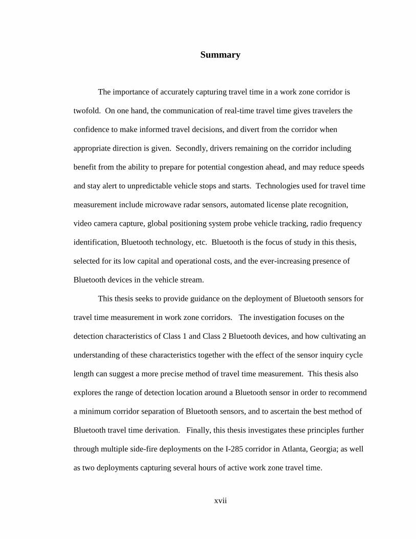
The importance of accurately capturing travel time in a work zone corridor is
twofold. On one hand, the communication of real-time travel time gives travelers the
confidence to make informed travel decisions, and divert from the corridor when
appropriate direction is given. Secondly, drivers remaining on the corridor including
benefit from the ability to prepare for potential congestion ahead, and may reduce speeds
and stay alert to unpredictable vehicle stops and starts. Technologies used for travel time
measurement include microwave radar sensors, automated license plate recognition,
video camera capture, global positioning system probe vehicle tracking, radio frequency
identification, Bluetooth technology, etc. Bluetooth is the focus of study in this thesis,
selected for its low capital and operational costs, and the ever-increasing presence of
Bluetooth devices in the vehicle stream.
This thesis seeks to provide guidance on the deployment of Bluetooth sensors for
travel time measurement in work zone corridors. The investigation focuses on the
detection characteristics of Class 1 and Class 2 Bluetooth devices, and how cultivating an
understanding of these characteristics together with the effect of the sensor inquiry cycle
length can suggest a more precise method of travel time measurement. This thesis also
explores the range of detection location around a Bluetooth sensor in order to recommend
a minimum corridor separation of Bluetooth sensors, and to ascertain the best method of
Bluetooth travel time derivation. Finally, this thesis investigates these principles further
through multiple side-fire deployments on the I-285 corridor in Atlanta, Georgia; as well
as two deployments capturing several hours of active work zone travel time.

1
Chapter 1: Introduction
Work zones provide several challenges to transportation agencies with respect to
traffic management and monitoring, protection of worker and driver safety, maintenance
of traffic flow, communication of existing conditions, and suggestion of alternative routes
to drivers. Many work zone corridors feature the integration of changeable message sign
(CMS) to inform drivers of expected delays and alternative routes; and an array of
vehicle detection technologies to capture and transmit vehicle speeds, volumes, and travel
times to a central database for disbursement to the traveling public.
The ability to transmit real-time speeds and travel times is of high importance in a
work zone because the drivers approaching and traversing the corridor are making route
choices based on the information provided to them. Delays associated with the capture
and transmission of vehicle travel time translate to a less accurate representation of the
current work zone corridor travel time (i.e. “stale” data), and thus less ideal driver
decisions. Furthermore, evidence shows that with the presentation of potential alternative
routes along with travel time data, motorists are more likely to divert their travel away
from the work zone corridor. Evidence on the I-65 work zone in Indiana showed a
diversion of 30% when alternative routes were displayed [30], along with 10% diversion
in a Texas work zone [34], and 53% responsiveness in Washington D.C [34].
Common intelligent transportation systems deployed in work zone corridors
include inductive loop sensors installed in pavement, microwave and radar sensors, and
video imaging. Vehicle detection systems on the rise include cell phone tracking,
2
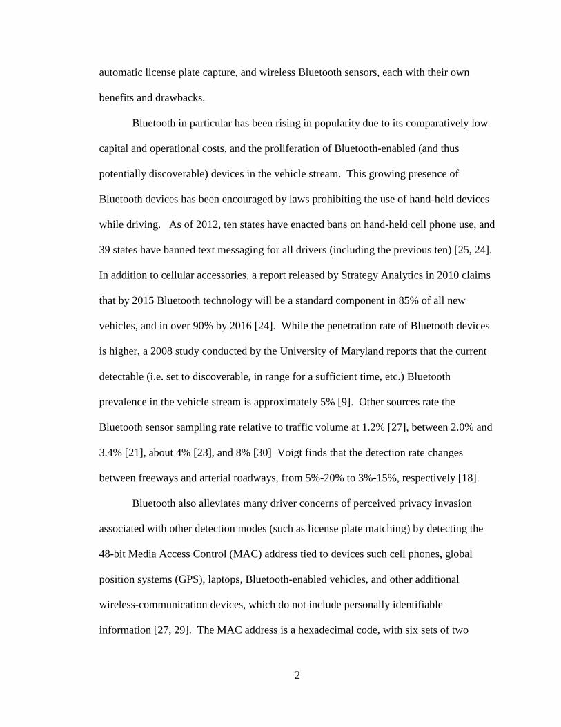
automatic license plate capture, and wireless Bluetooth sensors, each with their own
benefits and drawbacks.
Bluetooth in particular has been rising in popularity due to its comparatively low
capital and operational costs, and the proliferation of Bluetooth-enabled (and thus
potentially discoverable) devices in the vehicle stream. This growing presence of
Bluetooth devices has been encouraged by laws prohibiting the use of hand-held devices
while driving. As of 2012, ten states have enacted bans on hand-held cell phone use, and
39 states have banned text messaging for all drivers (including the previous ten) [25, 24].
In addition to cellular accessories, a report released by Strategy Analytics in 2010 claims
that by 2015 Bluetooth technology will be a standard component in 85% of all new
vehicles, and in over 90% by 2016 [24]. While the penetration rate of Bluetooth devices
is higher, a 2008 study conducted by the University of Maryland reports that the current
detectable (i.e. set to discoverable, in range for a sufficient time, etc.) Bluetooth
prevalence in the vehicle stream is approximately 5% [9]. Other sources rate the
Bluetooth sensor sampling rate relative to traffic volume at 1.2% [27], between 2.0% and
3.4% [21], about 4% [23], and 8% [30] Voigt finds that the detection rate changes
between freeways and arterial roadways, from 5%-20% to 3%-15%, respectively [18].
Bluetooth also alleviates many driver concerns of perceived privacy invasion
associated with other detection modes (such as license plate matching) by detecting the
48-bit Media Access Control (MAC) address tied to devices such cell phones, global
position systems (GPS), laptops, Bluetooth-enabled vehicles, and other additional
wireless-communication devices, which do not include personally identifiable
information [27, 29]. The MAC address is a hexadecimal code, with six sets of two

3
alpha-numeric pairs (i.e. a1:b2:c3:d4:e5:f6). The first three pairs provide information
regarding the device manufacturer, and can be used in identifying the type of Bluetooth
device, but there is no direct link available to the user [39]. One way that commercial
Bluetooth sensor developers respond further to the privacy concern is to only store the
last half of the MAC address, and encrypt the remainder of the address code.
A drawback to Bluetooth device detection for travel time calculation is the range
of error associated with location of the device relative to the sensor. Thus, the Bluetooth
sensors are not able to pinpoint the location of a device, and thus the exact location of
flow breakdown or any important information about individual vehicles in the traffic
stream. Although Bluetooth is a formidable technology for travel time measurement, by
itself it is unable to alleviate the additional concerns of work zone traffic management.
1.1 Problem Statement
The use of Bluetooth for measuring travel times in work zones is a relatively new
practice. Therefore, further investigation is needed as to the placement, spacing, and
design of Bluetooth sensors along a work zone corridor to provide the most accurate,
real-time measure of travel time possible within the limits of a construction project. The
issue of placement refers to where to position the sensors along a work zone corridor to
detect the greatest number of devices, most significantly the position relative to corridor
entrance and egress points. The issue of spacing refers to the distance separating the
Bluetooth sensors, and how shortening or widening the distance impacts the travel time
measurement error. Lastly, the design of Bluetooth sensors refers to the sensor inquiry
cycle impact on device detection along a corridor.

4
1.2 Objective
This objective of this thesis is to answer questions regarding the placement,
spacing, and design of Bluetooth sensors in a work zone corridor by specifically
exploring (1) how best to maximize the number of devices detected by a Bluetooth
sensor, with an understanding that more device detections will narrow the confidence
bounds surrounding the average travel time output; (2) how best to space the devices
along the corridor to minimize the effect of the range of detection location around a
Bluetooth sensor; and (3) how best to program the inquiry cycle period to achieve the
most accurate measure of real-time travel time. This thesis explores these parameters by
studying the detection characteristics of Class 1 and Class 2 Bluetooth devices; the
characteristics of Class 1 Bluetooth sensors; and the location where detection is occurring
around a Bluetooth sensor. The research then takes these lessons and applies them to a
side-fire deployment along a freeway, and finally to a live work zone setting.
1.3 Overview
This thesis begins by providing a review of the literature available pertaining to
Bluetooth technology, as well as a discussion of the current practice of travel time
measurement in work zones. Next, the thesis delves into the selection and configuration
of Bluetooth devices and equipment integrated into these research studies. Following the
discussion of equipment, the thesis describes the experimental design, an overview of the
parameters for data processing and analysis, and presents the results. The thesis wraps up
with concluding thoughts and the recommended next steps to expand the research focus.
5
Chapter 2: Literature Review
2.1 Overview of Work Zone Travel Time Applications
2.1.1 Methods of Measuring Travel Time in Work Zones
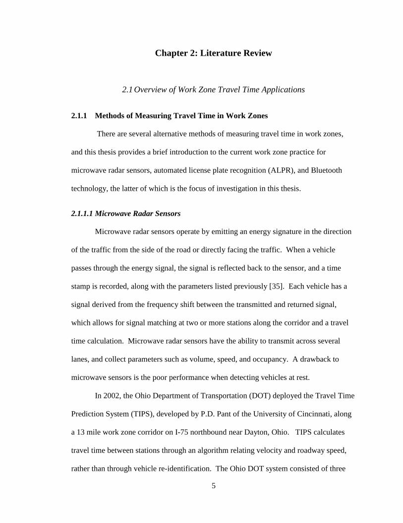
There are several alternative methods of measuring travel time in work zones,
and this thesis provides a brief introduction to the current work zone practice for
microwave radar sensors, automated license plate recognition (ALPR), and Bluetooth
technology, the latter of which is the focus of investigation in this thesis.
2.1.1.1 Microwave Radar Sensors
Microwave radar sensors operate by emitting an energy signature in the direction
of the traffic from the side of the road or directly facing the traffic. When a vehicle
passes through the energy signal, the signal is reflected back to the sensor, and a time
stamp is recorded, along with the parameters listed previously [35]. Each vehicle has a
signal derived from the frequency shift between the transmitted and returned signal,
which allows for signal matching at two or more stations along the corridor and a travel
time calculation. Microwave radar sensors have the ability to transmit across several
lanes, and collect parameters such as volume, speed, and occupancy. A drawback to
microwave sensors is the poor performance when detecting vehicles at rest.
In 2002, the Ohio Department of Transportation (DOT) deployed the Travel Time
Prediction System (TIPS), developed by P.D. Pant of the University of Cincinnati, along
a 13 mile work zone corridor on I-75 northbound near Dayton, Ohio. TIPS calculates
travel time between stations through an algorithm relating velocity and roadway speed,
rather than through vehicle re-identification. The Ohio DOT system consisted of three

6
CMSs, and microwave radar sensors placed at five stations along the roadway ranging
from 5.6 miles to 12.5 mile apart. The TIPS system displayed travel time in four minute
increments. For the 119 completed runs, the predicted travel time for the system ranged
from eight minutes to 36 minutes. The system reportedly had 88% of travel times
accurate to within four minutes, and a 65% to 71% of travel times accurate to within two
minutes [33].
During the same time period in summer 2001, a TIPS system was deployed in a
Wisconsin work zone on I-94 southbound. The traffic management system consisted of
two CMSs and five microwave radar sensors. The CMSs were placed three miles apart,
starting six miles before the start of the work zone. The first microwave radar sensor was
placed with the first CMS, with the next three placed in two mile increments up to the
construction taper, and last placed three miles into the work zone corridor for a total
corridor length of about 10.3 miles. This system displayed the travel time in four minute
increments, with the range of predicted travel times falling between 16 and 48 minutes
depending on the level of congestion. The results of this travel time output show that
travel times were within four minutes of the actual travel time 46% and 66% of the time
for the two CMSs used; and within 30% of actual travel times for 85% and 86% of all
observations for the two CMSs [36].
The Arkansas State Highway and Transportation Department also featured four
radar traffic microwave sensors (RTMS), each on the eastbound and westbound approach
ends of a 6.3 mile long work zone corridor, in the summer of 2002. The eastbound
sensors were placed along 7.8 miles before the east end of the work zone, and the
westbound sensors along 12.8 miles before the west end of the work zone. The RTMS

7
system proved difficult to calibrate due to the variable changing lane closure schedule, so
the RTMS was replaced by Doppler radar units to solve the calibration issues [28]. The
average free flow work zone travel times for the eastbound and westbound directions
were 12 minutes and 47 seconds, and 16 minutes and 50 seconds, respectively. The
displayed travel times were within five minutes of the actual travel time 90% of the time,
out of 144 total records.
2.1.1.2 Automated License Plate Recognition
ALPR devices operate by taking a picture of the license plates of passing vehicles
with either color, black-and-white, or infrared cameras. Each image capture is associated
with a time stamp and the GPS coordinates of the ALPR camera. The plate processing
follows the four steps: image acquisition, license plate extraction, license plate
segmentation, and character recognition. After the character recognition step the plate
has been transformed into a usable format (i.e. text file output) and may be matched at
various locations along the corridor to generation travel time measurements [37]. ALPR
cameras are typically used by law enforcement agencies, but have been on the rise as a
method of travel time measure. A drawback is the expense of the ALPR equipment and
processing system. One example of ALPR travel time collection in a work zone was in
Arizona in 2004. The Federal Highway Administration (FHWA) released a case study
following the use of a license plate matching system to manage traffic during the
reconstruction of 13.5 miles of Arizona State Route 68 [16]. The system was able to
successfully read 60% of the license plates and match 11% of the plates for travel time
readings. The system also immediately encrypted the license plates before archiving
them to allay the privacy concerns of the public.
8
2.1.1.3 Bluetooth Sensor Technology
The basic tenets of Bluetooth sensor operation include the sensor transmission of
an “inquiry” signal on an unlicensed radio frequency, and the simultaneous “scanning” of
radio frequencies by Bluetooth-enabled devices such as cell phones or navigation systems
within vehicles. Detection occurs when a Bluetooth-enabled device receives the message
from the Bluetooth sensor and responds with its unique MAC identifier, to which the
sensor attaches a time stamp and records in a log. Travel time is generated by matching
the MAC address of a Bluetooth-enabled device at different points along the corridor, and
taking a difference of the time stamps to derive a travel time measure. The details of
current Bluetooth practices in work zones, and an in-depth description of the Bluetooth
detection process and related properties are discussed in the following sections, and lay
the groundwork for the research presented in this thesis.
2.1.2 Previous Applications of Bluetooth to Measure Work Zone Travel Time
Bluetooth has become a prevalent technology for work zone travel time measure
due to its low capital and operational costs, a steadily increasing Bluetooth device
population, and Bluetooth’s ability to transmit over long-range distances of
approximately 100 meters (330 feet). There have been several cases of successful
Bluetooth travel time application in active work zones, such as in 2009 when the Indiana
DOT placed semi-permanent Bluetooth sensors along a ten mile work zone corridor on I-
65 atop CMSs, and portable units along alternative diversion routes around the work zone
(indicated to motorists through the CMSs) [30]. The Bluetooth sensors installed on the
CMSs provided a direct uplink in near-real-time to Indiana DOT’s Advanced Traveler
Information System; and the portable units stored data internally for later download and

9
post-processing. The processing of Bluetooth travel times enabled Hasemen, et al., in
2010, to note where the delay exceeded ten minutes, and to relate this to the development
of a queue [30].
In 2010, the Ontario Ministry of Transportation (MTO) in Canada deployed the
BluFax Bluetooth system to monitor traffic delay during the Fairchild Creek culvert
replacement project. Two BluFax units were placed 3 kilometers (km) on either side of
the bridge under construction for point to point travel time readings [17]. The findings of
travel time accuracy were not available for this study.
In 2010, Illinois DOT installed 22 Bluetooth sensor boxes designed by Trafficast
in a 27 mile work zone corridor along the Eisenhower Expressway [29]. The Bluetooth
sensors were employed to provide travel time information to motorists when the roadway
resurfacing impaired the in-pavement sensors that were the previous source of travel time
and congestion data. All accounts of this work zone are present in media records. Thus,
travel time accuracy results are not available for this study
Currently in 2012 the Texas A&M Transportation Institute designed and monitors
a travel information system for the I-35 expansion project; a 96 mile stretch from
Hillsboro to Salado in Texas. The traffic monitoring includes the integration of
Bluetooth sensors for travel time, Wavetronix systems for volume, and radar systems for
speed measurement to judge the build-up of queues before the work zone entrance [32].
As this study is currently underway, findings are not available at this time.
2.1.3 Advantages and Disadvantages of Bluetooth in Work Zones
A Portland, Oregon Pilot Study recognizes several advantages of Bluetooth
including its ability to provide accurate ground truth data without having to add probe

10
vehicles into the system, the ability to provide a wireless communication link between the
Bluetooth system and an online server for real-time travel data transmission, and the
relative low cost of Bluetooth technology compared to the alternative license plate
readers and in-road loop detectors [5]. A study by the University of Maryland in 2008
estimated that Bluetooth technology was 500 to 2500 times more economical (i.e. less
expensive) than equipping probe vehicles to obtain the same number of data points [9].
Hasemen, et al., similarly finds that alternatives to Bluetooth such as license plate
matching and probe vehicles are “prohibitively expense” [30]. Furthermore, Bluetooth
detection does not require a direct line of sight from the sensor to the device, and can also
travel through most physical barriers, according to a 2001 study by Bringham Young
University [10]. However, limited research by Kittelson and Associates, Inc. finds that
despite being penetrable, the presence of a car door may decrease the detection radius of
the sensor by as much as half due to interference [5].
Some disadvantages of Bluetooth technology include the need for an exterior
power source for extended periods of operation, as well as the inability of Bluetooth to
detect vehicle trajectories and point speeds [5]. Additional obstacles of Bluetooth system
operation identified in a Portland, Oregon Pilot Study include the interference from
stationary nearby devices, devices traveling on alternative routes, as well as
complications that arise from the internal computer clock drift and detection ping cycles
[5].
2.2 Overview of Bluetooth Technology
Bluetooth is a method of wireless device communication operating on the
Industrial, Scientific, and Medical (ISM) unlicensed radio frequency band of 2.4000

11
Gigahertz (GHz) to 2.4835 GHz, which is the same frequency band for the
communication of wireless cordless phones and other wireless devices [12]. The 2.4
GHz frequency band consists of 79 1-Megahertz (MHz) channels from 2402 to 2480
MHz, across which a Bluetooth signal will “hop” in a randomly defined order, making
changes up to 1,600 times per second (or once every 625 micro-seconds (µs)) [6, 13].
The hopping sequence of Bluetooth transmission, formally called the Frequency Hopping
Spread Spectrum (FHSS), occurs to minimize the likelihood of interference with other
Bluetooth signals competing for communication along the same 2.4 GHz frequency band
[6].
According to the Federal Communication Commission (FCC) sections 15.247 and
15.249 there are certain criteria that frequency hopping on the 2.4 GHz band must meet.
These include a random hopping pattern across at least 15 non-continuous frequency
channels, and being stationary at a given frequency no longer than 0.4 seconds multiplied
by the number of frequency channels [7]. Of the 79 hopping frequencies available on the
unlicensed spectrum, 32 are used for inquiry (called “wake-up frequencies”), and another
32 are used for inquiry response based on the Bluetooth versions for the United States
and most European countries [3, 2, 14].
2.2.1 Sensor-Device Inquiry Protocol
2.2.1.1 Procedure
The inquiry protocol establishing the sensor-device interaction is initiated by a
master device, and received by a slave device. The master device sends out an inquiry
packet of information on the 2.4 GHz frequency band in search of Bluetooth-enabled
devices, or slaves. The protocol established the master and slave because one device is
12
controlling the communication (the master) and other device is responding to and
following the directions of the master device (the slave). The roles may also be reversed
at any time.
There are two major states and are seven substates that devices can fall under
during the device connection process. The two major states are standby and connection.
The substates vary depending on whether a device is a master device or a slave device,
and consist of the following: (1) inquiry (master); (2) inquiry scan (slave) (3) inquiry
response (slave); (4) page (master); (5) page scan (slave); (6) slave response (slave); (7)
master response (master) [1, 2, 10, 12]. Following the final master and slave responses, a
connection is initiated between the two devices.
The first initiation of connection protocol is when a master device enters the
inquiry substate. The inquiring device generates a hopping sequence based on an inquiry
access code (IAC), and the inquiring device’s internal clock, which determines the phase
in the hopping sequence [10, 12]. The IAC may be general (GIAC) if the inquirer wishes
to discover all devices in range, or dedicated (DIAC) if the inquirer wishes to find
specific types of devices (or different device classes) [11, 12]. The inquiring device then
broadcasts a message or ID packet over the 32 wake-up frequencies of the 2.4 GHz
frequency band in the pre-determined hopping sequence, which is simply a packet
containing an access code, packet header, and payload [11]. Every time the inquiry hops
to the next frequency it transmits two ID packets, one of which the receiving device
should register when it hops to the same frequency. Each ID packet is 625 µs in length,
or one time slot. During the inquiry phase the ID packet lengths are reduced to 312.5 µs
half slots.

13
The 32 inquiry channels are separated in two unique 16 channel trains, and there
must be two iterations of each train during the inquiry process. The inquiry message first
transmits over the first set of 16 frequencies, repeating 256 times, and then transmits over
the second set of 16 frequencies. During the inquiry state the hopping rate increases from
1600 hops per second to 3200 hops per second for the inquirer to increase the likelihood
of a connection [12]. The faster inquiry rate is what allows for the 312.5 half-slot during
frequency hopping. The inquiry substate proceeds continuously until it receives a
response from a potential slave device.
The second substate for a device to enter is the inquiry scanning substate, which a
device must be in to receive the inquiry packet transmitted from the master device. The
potential slave device is not always active, but rather is in the standby state and will
periodically enter the inquiry scan state and hop on the 32 wake-up frequencies. The
scanning frequency hopping sequence takes place at a much slower rate, changing
frequencies every 1.28 seconds (remaining for 2048 time slots on each frequency band)
[12, 14, 15]. The inquiry scanning substate follows the same frequency hopping
mechanism described above, which is determined instead by the internal clock of the
scanning device, and the device access code. Just as for the inquiring device, the
scanning device hops across the 32 frequencies between two sets of 16-frequency trains.
The third substate is the inquiry response substate, which a device enters after
scanning the frequencies and receiving an ID packet from the master device. The device
then sends an inquiry response message, or Frequency Hopping Synchronization (FHS)
packet, which includes the device’s native clock and a 48-bit Bluetooth Device Address
(BD_ADDR). Once again, this packet covers a single time slot, or 625 µs. The FHS
14
packet informs the potential master device what hopping sequence the local device is
following, so the master device can use that sequence for the next communication.
However, the receiving device does not send the FHS packet right away. Instead, the
device halts the inquiry process for a time period of x time slots, randomly selected from
0 to 1023 (a maximum of 639.375 milliseconds (ms)) [3]. This period is called the back-
off limit, and adds to the average total delay in device discovery [14]. This back-off time
minimizes the potential for a signal collision with other devices that may be responding
to the same master inquiry ID packet. After this random interval expires, the local device
sends the FHS packet when it receives the next inquiry message from the master device
[12, 3].
After the receiving device sends the FHS packet to the inquiring device, there is a
period of delay, referred to as frequency synchronization (FS) delay, before the potential
master begins to transmit using the frequency hopping sequence delivered in the FHS
packet. Once the potential master receives the FHS packet, it enters the page substate. In
the page substate, the potential master sends a Device Access Code (DAC) packet to the
potential slave, which should be in the page scan substate. The inquirer sends the DAC
packet using a frequency hopping sequence determined by the FHS packet sent by the
potential slave, which is based off the local device’s address and local clock. The DAC
packet contains unique information about the master device, allowing the potential slave
device to request access to the master device.
Meanwhile, the potential slave device entered the page scan substate after sending
the first FHS packet response to the potential master device. In the page scan substate,
15
the potential slave device hops according to the internal clock and local device address
[1].
When the potential slave device receives the DAC packet from the master device,
it responds with a DAC packet, or page response packet. Immediately upon receiving the
return DAC packet from the potential slave device, the master device sends an FHS
packet to the local device, which contains the master device’s native clock and
BD_ADDR. After receiving the FHS packet, the potential slave device adjusts its
hopping frequency to match that of the master device, and sends an additional reply DAC
packet. After receiving the final DAC packet, a connecting is initiated and the master
device controls the communication with the slave device. This connection is called a
piconet, which can be point to point, or point to multipoint [19]. Multiple piconets
together make up a scatternet. Now that the inquiry has completed, the master device
reduces its hop rate from 32000 hops per second to 1600 hops per second, and the slave
device increases its hop rate the same rate for matching communication [10, 3, 12].
Figure 1 below provides a summary of the device-sensor inquiry process.

16
Figure 1 Device-Sensor Inquiry Protocol Procedure [14]
2.2.1.2 Inquiry Cycle Length
There are many elements that contribute to the industry standard, and Bluetooth-
recommended specification of a 10.24 second inquiry cycle. The inquiry cycle is
designed as the optimal time needed to detect all discoverable Bluetooth devices within
range. The Bluetooth specifications recommend completing two iterations of each 16-
frequency train, and repeating the entire inquiry process 256 times. The 256 repetitions
come from 16 multiplied by 16, to cover all frequency pairings between the potential
master and slaves alternating between the two 16-frequency trains. The 10.24 second

17
inquiry cycle is derived from the following formula: 2 trains × 0.01 second/train × 2
iterations × 256 repetitions = 10.24 seconds [10].
A study by Peterson, et al., in 2006 recommends that an inquiry cycle should be
limited only to detect an “acceptable number of devices” [15]. Their study suggests that
a single sensor will detect 98.95% of scanning devices in 5.12 seconds. The study further
suggests that the inquiry method can be reduced to 3.84 and 1.28 seconds using standard
and interlaced inquiry modes [15]. Figure 2 below provides a summary of Peterson, et
al.’s inquiry length investigation. Chakraborty, et al., also finds that two devices
typically take 5.76 seconds to establish a connection [14]. Another component to device
inquiry is the capacity of a sensor for detection. Voigt identifies a limit of eight MAC
address reads per second [18].
Figure 2 Summary of Inquiry Duration Investigation by Peterson, et al. [15]
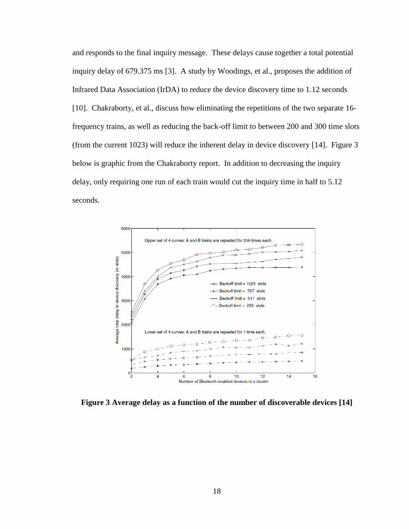
An additional factor influencing the total detection time is the delay inherent in
the detection process. Zaruba, et al., identifies the total inquiry delay as a function of the
FS delay and random back-off delay. The first FS delay occurs in the initial inquiry
substate when the master sends the first IAC to the potential slave. The second FS delay
is the time it takes after the potential slave wakes up from its back-off, to when it receives
18
and responds to the final inquiry message. These delays cause together a total potential
inquiry delay of 679.375 ms [3]. A study by Woodings, et al., proposes the addition of
Infrared Data Association (IrDA) to reduce the device discovery time to 1.12 seconds
[10]. Chakraborty, et al., discuss how eliminating the repetitions of the two separate 16-
frequency trains, as well as reducing the back-off limit to between 200 and 300 time slots
(from the current 1023) will reduce the inherent delay in device discovery [14]. Figure 3
below is graphic from the Chakraborty report. In addition to decreasing the inquiry
delay, only requiring one run of each train would cut the inquiry time in half to 5.12
seconds.
Figure 3 Average delay as a function of the number of discoverable devices [14]

19
2.2.2 Bluetooth Class and Model Specifications
Since the first Bluetooth specifications released in 1999 there have been many
new standards created for the development of Bluetooth-enabled products. Over the
years, Bluetooth has seen the addition of the adaptive frequency hopping (AFH) feature,
which allows the Bluetooth inquiry frequency hopping pattern to avoid frequencies with a
fixed interference stream. Additional features include an enhanced data rate (EDR)
transfer, which increases the base information transfer speed from 1 Megabit per second
(Mbps) to 3 Mbps. The more realistic data transfer rate for Class 1 and Class 2 devices is
721 Kilobits per second (kbps) and 2.1 Mbps, respectively [4]. The EDR feature is
present in Bluetooth model specifications 2.0 and forward, with version 1.2 and prior
having the slower data transmission speed of 1 Mbps [22, 6]. The most recent Bluetooth
model specifications allow for a data transfer rate upwards of 10 Mbps.
Bluetooth-enabled devices also fall under a power class of 1, 2, or 3, with Class 1
being the highest power class and Class 3 being the lowest power class. The power class
represents the amount of power draw the device requires for operation, measured as
1milliwatt (mW) (0 decibels (dBm)) for Class 3 devices, 2.5 mW (4 dBm) for Class 2
devices, and 100 mW (20 dBm) for Class 1 devices. The dBm represents the power ratio
in decibels to mW. A compliance overview published by Texas Instruments in 2005, and
SEMTECH International’s overview of FCC regulations for ISM Band devices, list that
FCC sections 15.247 and 15.249 put the maximum power at +21 dB with 15 to 75
frequency hopping channels [7, 8]. However, with frequency hopping in place, and
greater than 75 hopping channels, power can be a maximum of +30 dB.
20
The power requirements for the different Bluetooth classes correlate with the
transmission range of the power class. Class 1 Bluetooth-enabled devices experience the
greatest transmission range of approximately 100 meters (330 feet), followed by Class 2
at 10 meters (33 feet), and Class 3 at 1 meter (3 feet) [19]. Higher power devices such as
laptops, tablets, and specially designed adaptor plug-ins typically fall under the Class 1
rating and allow for transmission of data over a much farther range than their Class 2
counterparts found in Bluetooth headsets, hand-held GPS devices, et cetera. Class 3
Bluetooth devices are much less common, and therefore the focus of the research
investigation in this thesis revolves around Class 1 and Class 2 devices.
Therefore, the performance and characteristics of any Bluetooth-enabled device
within the discoverable population of a Bluetooth sensor is defined by the Bluetooth
specification guidelines, which determines the transmission speed and adaptability; and
the Bluetooth power class, which determines the transmission range. Knowing the range
of properties a detectable population is expected to exhibit allows for the proper design of
a Bluetooth sensor system.
2.2.3 Bluetooth Detection Range
The typical range of Class 1 Bluetooth sensor is approximately 330 feet. As such,
a Bluetooth-enabled device must be within the 330 foot radius surrounding a Bluetooth
sensor if it is to be detected. The detection between device and sensor can be likened to
two men standing on a football field; one at an end zone and one at midfield [19]. If the
two men are both Class 1 devices then as one man shouts to the other across a 330 foot
distance, the sound will make it to the second man, and he will be able to detect the
communication and return a shout back across the field for the first man to receive.

21
However, if the first man is a “Class 2 device” then when he attempts to shout to the
second man down the field, the shout will only travel approximately 33 feet (not far
enough for the second man to receive the communication and respond). This analogy
helps explain the boundaries of the communication between Class 1 and Class 2
Bluetooth-enabled devices, and that the communication range is limited by the weaker
power class [19]. As an example, the XRange2000 Bluetooth transmitter product has an
advertised range of 1000 to 2000 meters, but a real-application communication range of
up to 250 meters, limited by the capabilities of the cell phones on the receiving end [20].
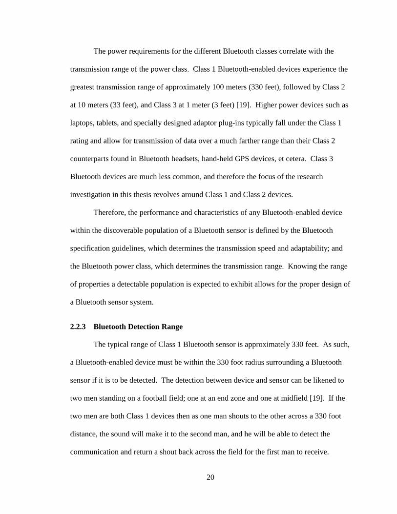
A study completed by Motorola on Bluetooth radio performance in 2008
describes an alternative view of the real Bluetooth device range. The Motorola Technical
Brief states that the Bluetooth device range is a combination of the radio frequency (RF)
power of the transmitter, the receiver sensitivity, and the absorption rate of the medium
the transmission is attempting to travel through [6]. According to this analysis, detection
range is function of the maximum allowable path loss, which is the difference between
the maximum device power, and the maximum device sensitivity, which is independent
of whether the Bluetooth device is power class 1 or 2. Note Figure 4 below, from the
Motorola Technical Brief, which provides a visual representation of the principle just
described. This shows that Class 1 and Class 2 Bluetooth devices can theoretically have
the same transmission range. Thus, by supplying a Class 2 device with a greater
sensitivity, the maximum power loss is increased, thus increasing the transmission range.

22
Figure 4 Class 1 and Class 2 Bluetooth Radio Performance [6]
2.2.4 Bluetooth Travel Time and Speed Error
J. Porter, et al., cites the result of a Virginia DOT study that capturing between
2% and 3% of the total roadway traffic volume (three samples every five minutes) is
acceptable for generation of a meaningful travel time measure [23]. Monsere, et al.,
reports that travel time estimates that fall within 20% of the actual travel time can still
provide useful information to motorists, and that this error value is deemed acceptable by
the FHWA [26]. Tudor, et al., finds that a travel time delay error of five minutes was
acceptable for a 7.8 and 12.8 mile work zone corridor in the study of smart work zone
technology in Arkansas (with approximate 13 minute and 17 minute respective free flow
travel times). Several motorists still filed complaints that this margin was too great [28].
Malinovskiy, et al., conducted a field test on a 0.98 mile corridor comparing the
performance of Bluetooth and ALPR technologies for time travel measurement.
23
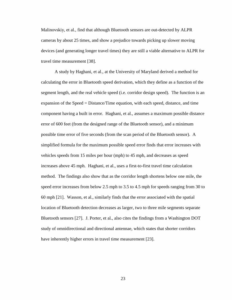
Malinovskiy, et al., find that although Bluetooth sensors are out-detected by ALPR
cameras by about 25 times, and show a prejudice towards picking up slower moving
devices (and generating longer travel times) they are still a viable alternative to ALPR for
travel time measurement [38].
A study by Haghani, et al., at the University of Maryland derived a method for
calculating the error in Bluetooth speed derivation, which they define as a function of the
segment length, and the real vehicle speed (i.e. corridor design speed). The function is an
expansion of the Speed = Distance/Time equation, with each speed, distance, and time
component having a built in error. Haghani, et al., assumes a maximum possible distance
error of 600 feet (from the designed range of the Bluetooth sensor), and a minimum
possible time error of five seconds (from the scan period of the Bluetooth sensor). A
simplified formula for the maximum possible speed error finds that error increases with
vehicles speeds from 15 miles per hour (mph) to 45 mph, and decreases as speed
increases above 45 mph. Haghani, et al., uses a first-to-first travel time calculation
method. The findings also show that as the corridor length shortens below one mile, the
speed error increases from below 2.5 mph to 3.5 to 4.5 mph for speeds ranging from 30 to
60 mph [21]. Wasson, et al., similarly finds that the error associated with the spatial
location of Bluetooth detection decreases as larger, two to three mile segments separate
Bluetooth sensors [27]. J. Porter, et al., also cites the findings from a Washington DOT
study of omnidirectional and directional antennae, which states that shorter corridors
have inherently higher errors in travel time measurement [23].
24
2.3 Summary
The literature discusses how Bluetooth is an up-and-coming technology for travel
time measurement in work zone corridors. There are several advantages of Bluetooth
technology such as the low cost and the proliferation of discoverable Bluetooth devices.
Some disadvantages include the inability to detect point speeds and the potential
interference from devices on adjacent corridors. A Bluetooth connection consists of a
master device, which initiates device communication through an inquiry process and
controls the communication; and a slave device, which response to the commands of the
master device. The roles may be reversed at any time. The Bluetooth specification states
that an inquiry cycle length of 10.24 seconds is necessary to detect all discoverable
devices within range of a Bluetooth sensor, but additional sources comment that a cycle
as short as 5.12 seconds is adequate. Furthermore, Bluetooth devices fall under different
power class ratings, which correspond to the speed and distance over which devices can
communicate. Higher power class devices (Class 1) have a greater transmission speed
and range than lower class devices (Class 2), by about three times. The properties of
detection range influence the error associated with a Bluetooth travel time measurement.
To reduce this travel time measurement error, many sources concur that a sensor
separation of greater than one mile, preferably two to three miles, should be maintained
along a corridor.
The following chapters of this thesis explore Bluetooth technology further in
multiple deployments in a live work zone environment on I-285 in Atlanta Georgia, as
well as in several comparison deployments along I-285 in a non-active work zone. This
thesis also investigates the 10.24 cycle length to assess whether the length is adequate to

25
detect a sufficient number of devices entering a sensor’s field of view. Furthermore, the
following chapters examine the detection properties of Class 1 and Class 2 devices, as
well as the detection range trends of these two power classes, and finally the resulting
error in Bluetooth travel time associated with this range error. The next chapter, Chapter
3, provides details on the devices and equipment selected for this research study, and
their method of configuration.

26
Chapter 3: Device and Equipment Selection and Configuration
3.1 Selection of Bluetooth Enabled Devices
Bluetooth-enabled devices played a large role in the research contained within
this thesis. They were first used as subjects in a controlled indoor test measuring sensor
capacity, cycle detection pattern, and detection headway by device power class. Their
second use was to serve as components of a known device population within probe
vehicles during field deployments. Details of the test deployments are described in
Chapter 4. The selection of Bluetooth-enabled devices to include in this study was driven
by the need to provide a realistic representation of the devices existing in a typical device
population. The knowledge that both Class1 and Class 2 devices are present in the traffic
stream underscored the importance of investigating their properties and detection
behavior in separate groups.
3.1.1 Class 1 Bluetooth-Enabled Devices
The research presented in this thesis includes four different Class 1 Bluetooth-
enabled devices. The devices are Asus Eee PC Netbooks, Toshiba Thrive AT-100
Tablets, and IOGear USB Bluetooth Adapters (plugged into Asus Netbooks to provide a
power source). An additional device used for the indoor control test series is an Apple
Mac Mini, Model #A1347, © 2010, referred to as rg49mac1. Table 1 provides a
summary of the Class 1 Bluetooth specifications and anticipated transmission range and
speed. Figure 5 and Figure 6 also show images of the Asus netbook and Toshiba Thrive
AT-100 tablet, respectively.

27
Table 1 Summary of Class 1 Device Specifications
Bluetooth
Version
Power
Class Frequency
Data
Transfer
Rate
Transmission
Range
(anticipated)
IOGear USB
Bluetooth Adapter 2.0 + EDR Class 1 2.4 GHz 2.1 Mbps 330 feet
Asus Eee PC
Netbook 2.1 + EDR Class 1 2.4 GHz 2.1 Mbps 330 feet
Toshiba Thrive
AT-100 Tablet 2.1 + EDR Class 1 2.4 GHz 2.1 Mbps 330 feet
Apple Mac Mini,
Model #A1347, ©
2010
2.1 + EDR Class 1 2.4 GHz 3.1 Mbps 330 feet
(a)
(b)
Figure 5 (a) IOGear Adapter connected to Asus netbook and (b) close-up of IOGear
adapter with MAC ID stamp
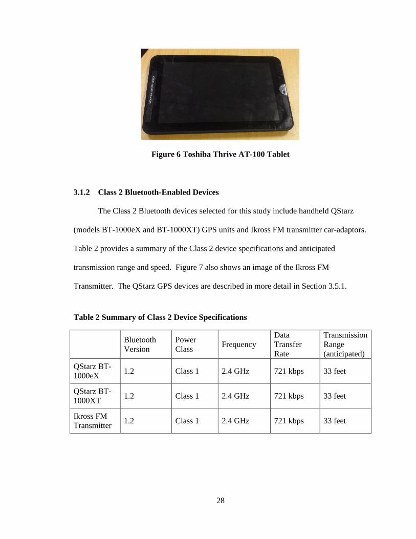
28
Figure 6 Toshiba Thrive AT-100 Tablet
3.1.2 Class 2 Bluetooth-Enabled Devices
The Class 2 Bluetooth devices selected for this study include handheld QStarz
(models BT-1000eX and BT-1000XT) GPS units and Ikross FM transmitter car-adaptors.
Table 2 provides a summary of the Class 2 device specifications and anticipated
transmission range and speed. Figure 7 also shows an image of the Ikross FM
Transmitter. The QStarz GPS devices are described in more detail in Section 3.5.1.
Table 2 Summary of Class 2 Device Specifications
Bluetooth
Version
Power
Class Frequency
Data
Transfer
Rate
Transmission
Range
(anticipated)
QStarz BT-
1000eX 1.2 Class 1 2.4 GHz 721 kbps 33 feet
QStarz BT-
1000XT 1.2 Class 1 2.4 GHz 721 kbps 33 feet
Ikross FM
Transmitter 1.2 Class 1 2.4 GHz 721 kbps 33 feet

29
Figure 7 Ikross FM Transmitter
3.2 Bluetooth Sensor Configuration
This thesis discusses the configuration of both a custom Bluetooth sensor
developed for this effort and commercial Bluetooth sensors. The custom Bluetooth
sensor system was developed by the Georgia Tech research team early in 2011. The
commercial Bluetooth system was purchased from Digiwest in summer 2012, and
operates using BlueMAC software with a wireless uplink to an online tracking database.
Digiwest was deployed in all Bluetooth deployments in hopes of providing a commercial
ruggedized alternative for travel time measurement in a work zone. However, at the time
of deployment the system did not perform as expected, so a travel time comparison was
not possible. Additional efforts are underway to determine if the commercial deployment
issue was related to user error or equipment malfunction.
3.2.1 Custom Class 1 Bluetooth Sensor
The custom sensor configuration is comprised of five components: (1) one
IOGear universal serial bus (USB) Bluetooth adaptor, (2) one ASUS netbook running a

30
Ubuntu Linux operating system, (3) one 32 foot USB extension cable providing a
connection between the IOGear adaptor and ASUS netbook, (4) one ten foot tall tripod
assembly consisting of a vertical body shaft and a three foot long perpendicular arm, and
(5) one 3/4 inch male PVC adaptor providing a secure, immobile connection between the
tripod arm and adaptor/extension cable joint. The sensor is designed to be mounted at a
ten foot height, based on the findings presented in Box’s 2011 thesis that a ten foot
antennae height will have the greatest detection rate [40]. Below, Figure 8 shows the
custom sensor configuration and Figure 9 shows a close-up of the PVC adaptor
connection to the tripod arm with the attached IOGear USB Bluetooth adapter.
Figure 8 Typical custom Bluetooth sensor configuration
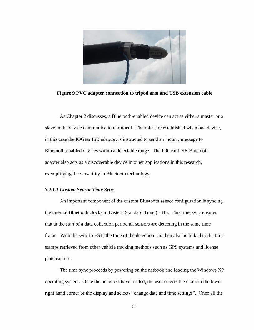
31
Figure 9 PVC adapter connection to tripod arm and USB extension cable
As Chapter 2 discusses, a Bluetooth-enabled device can act as either a master or a
slave in the device communication protocol. The roles are established when one device,
in this case the IOGear ISB adaptor, is instructed to send an inquiry message to
Bluetooth-enabled devices within a detectable range. The IOGear USB Bluetooth
adapter also acts as a discoverable device in other applications in this research,
exemplifying the versatility in Bluetooth technology.
3.2.1.1 Custom Sensor Time Sync
An important component of the custom Bluetooth sensor configuration is syncing
the internal Bluetooth clocks to Eastern Standard Time (EST). This time sync ensures
that at the start of a data collection period all sensors are detecting in the same time
frame. With the sync to EST, the time of the detection can then also be linked to the time
stamps retrieved from other vehicle tracking methods such as GPS systems and license
plate capture.
The time sync proceeds by powering on the netbook and loading the Windows XP
operating system. Once the netbooks have loaded, the user selects the clock in the lower
right hand corner of the display and selects “change date and time settings”. Once all the

32
netbooks are on this page, the user changes the netbook time according to the known EST
obtained via a cell phone or network-connected computer, with accuracy to the nearest
second. Software has since been developed to sync the netbooks with greater accuracy,
but was not available for the data collection efforts undertaken in this research.
Conducting a time sync before every Bluetooth deployment is recommended because the
internal netbook clock experiences a positive drift in time as the netbook is in operation.
The internal drift is small, observed as a drift of four seconds over an eight hour period of
operation (or 0.5 seconds per hour).
3.2.2 Digiwest Commercial Sensor
The Digiwest Bluetooth system is designed as a pole mount system. For the
purpose of this thesis, the pole mounting system was not possible, due to the long time
necessary to process an approval for access to a pole, the temporary nature of the
deployments, and the poor chance of a pole existing where the deployment was to take
place. Therefore, a tripod mounting system was designed to accommodate the Digiwest
Bluetooth sensor. With the battery installed in the unit, the weight of a single system is
approximately 15 pounds, so a very sturdy system was needed to support the unit at a ten
foot height and insure that the vertical arms do not sway. Figure 10 shows the front and
back views of the final configuration, which consists of two three-legged tripods with ten
foot vertical body shafts connected by two PVC arms onto which the Digiwest unit is
secured.
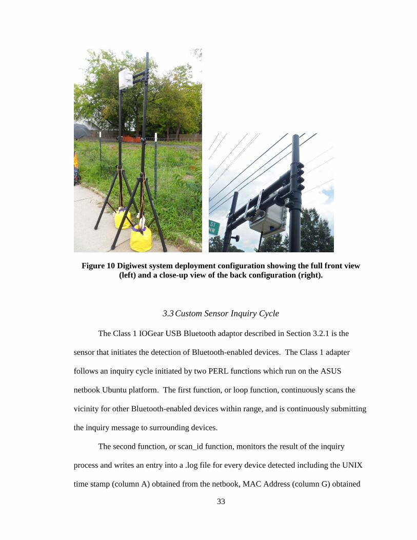
33
Figure 10 Digiwest system deployment configuration showing the full front view
(left) and a close-up view of the back configuration (right).
3.3 Custom Sensor Inquiry Cycle
The Class 1 IOGear USB Bluetooth adaptor described in Section 3.2.1 is the
sensor that initiates the detection of Bluetooth-enabled devices. The Class 1 adapter
follows an inquiry cycle initiated by two PERL functions which run on the ASUS
netbook Ubuntu platform. The first function, or loop function, continuously scans the
vicinity for other Bluetooth-enabled devices within range, and is continuously submitting
the inquiry message to surrounding devices.
The second function, or scan_id function, monitors the result of the inquiry
process and writes an entry into a .log file for every device detected including the UNIX
time stamp (column A) obtained from the netbook, MAC Address (column G) obtained
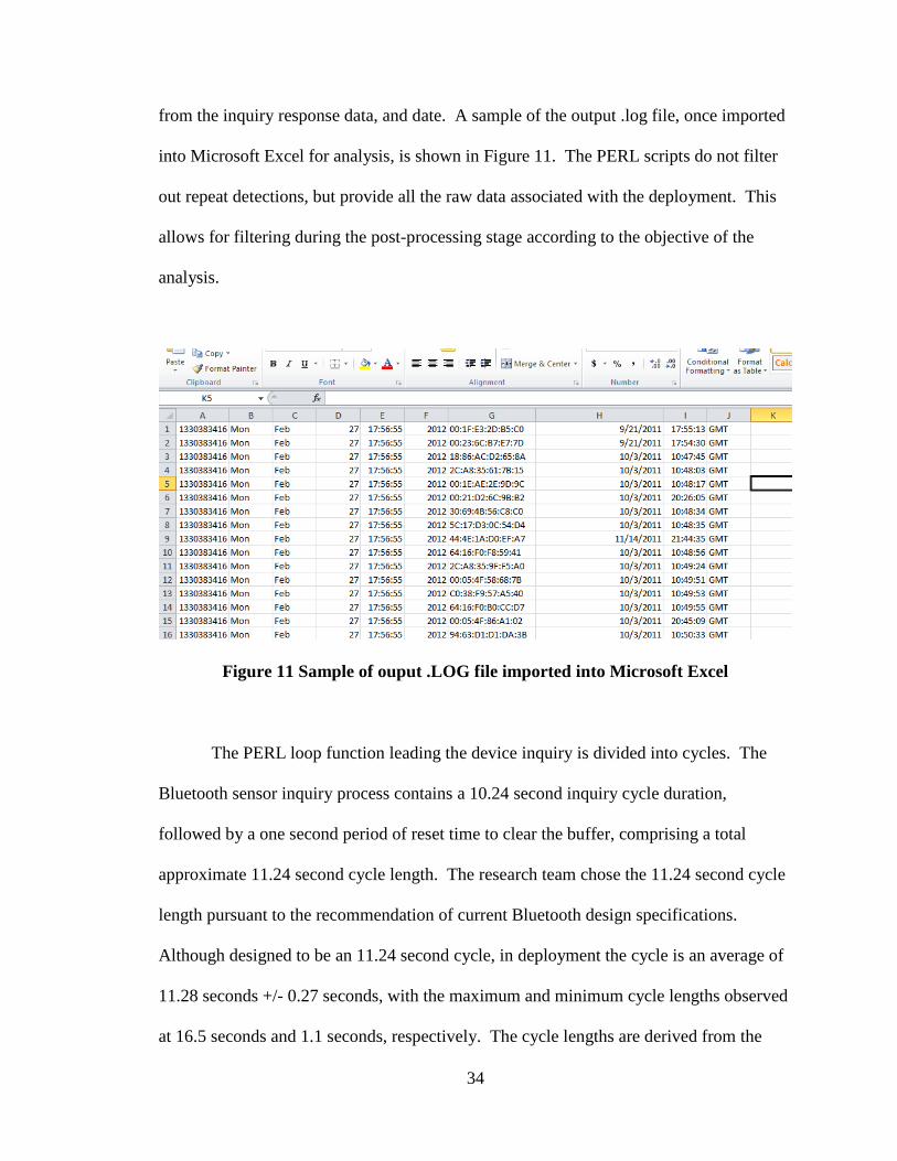
34
from the inquiry response data, and date. A sample of the output .log file, once imported
into Microsoft Excel for analysis, is shown in Figure 11. The PERL scripts do not filter
out repeat detections, but provide all the raw data associated with the deployment. This
allows for filtering during the post-processing stage according to the objective of the
analysis.
Figure 11 Sample of ouput .LOG file imported into Microsoft Excel
The PERL loop function leading the device inquiry is divided into cycles. The
Bluetooth sensor inquiry process contains a 10.24 second inquiry cycle duration,
followed by a one second period of reset time to clear the buffer, comprising a total
approximate 11.24 second cycle length. The research team chose the 11.24 second cycle
length pursuant to the recommendation of current Bluetooth design specifications.
Although designed to be an 11.24 second cycle, in deployment the cycle is an average of
11.28 seconds +/- 0.27 seconds, with the maximum and minimum cycle lengths observed
at 16.5 seconds and 1.1 seconds, respectively. The cycle lengths are derived from the
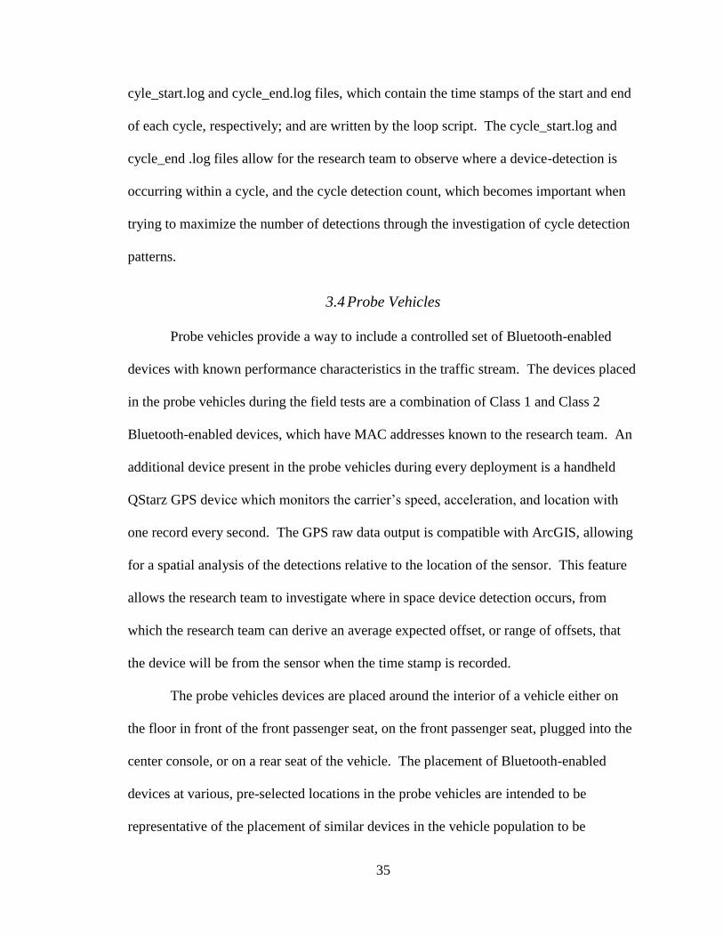
35
cyle_start.log and cycle_end.log files, which contain the time stamps of the start and end
of each cycle, respectively; and are written by the loop script. The cycle_start.log and
cycle_end .log files allow for the research team to observe where a device-detection is
occurring within a cycle, and the cycle detection count, which becomes important when
trying to maximize the number of detections through the investigation of cycle detection
patterns.
3.4 Probe Vehicles
Probe vehicles provide a way to include a controlled set of Bluetooth-enabled
devices with known performance characteristics in the traffic stream. The devices placed
in the probe vehicles during the field tests are a combination of Class 1 and Class 2
Bluetooth-enabled devices, which have MAC addresses known to the research team. An
additional device present in the probe vehicles during every deployment is a handheld
QStarz GPS device which monitors the carrier’s speed, acceleration, and location with
one record every second. The GPS raw data output is compatible with ArcGIS, allowing
for a spatial analysis of the detections relative to the location of the sensor. This feature
allows the research team to investigate where in space device detection occurs, from
which the research team can derive an average expected offset, or range of offsets, that
the device will be from the sensor when the time stamp is recorded.
The probe vehicles devices are placed around the interior of a vehicle either on
the floor in front of the front passenger seat, on the front passenger seat, plugged into the
center console, or on a rear seat of the vehicle. The placement of Bluetooth-enabled
devices at various, pre-selected locations in the probe vehicles are intended to be
representative of the placement of similar devices in the vehicle population to be
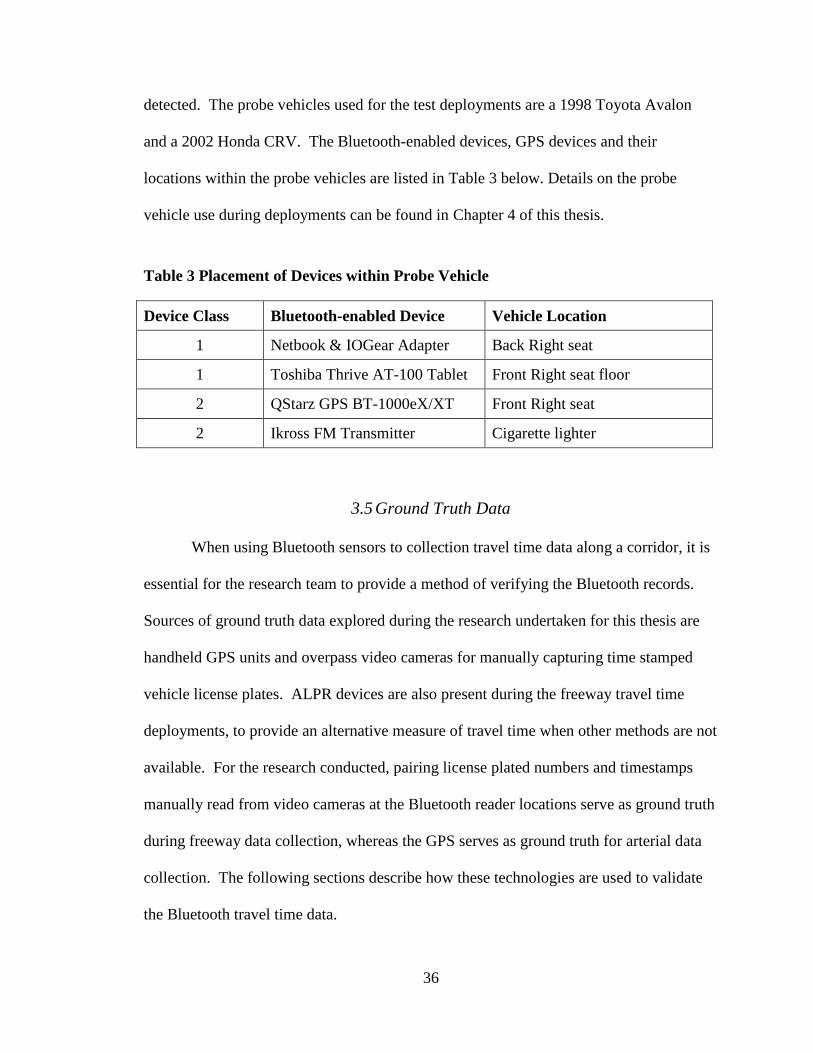
36
detected. The probe vehicles used for the test deployments are a 1998 Toyota Avalon
and a 2002 Honda CRV. The Bluetooth-enabled devices, GPS devices and their
locations within the probe vehicles are listed in Table 3 below. Details on the probe
vehicle use during deployments can be found in Chapter 4 of this thesis.
Table 3 Placement of Devices within Probe Vehicle
Device Class Bluetooth-enabled Device Vehicle Location
1 Netbook & IOGear Adapter Back Right seat
1 Toshiba Thrive AT-100 Tablet Front Right seat floor
2 QStarz GPS BT-1000eX/XT Front Right seat
2 Ikross FM Transmitter Cigarette lighter
3.5 Ground Truth Data
When using Bluetooth sensors to collection travel time data along a corridor, it is
essential for the research team to provide a method of verifying the Bluetooth records.
Sources of ground truth data explored during the research undertaken for this thesis are
handheld GPS units and overpass video cameras for manually capturing time stamped
vehicle license plates. ALPR devices are also present during the freeway travel time
deployments, to provide an alternative measure of travel time when other methods are not
available. For the research conducted, pairing license plated numbers and timestamps
manually read from video cameras at the Bluetooth reader locations serve as ground truth
during freeway data collection, whereas the GPS serves as ground truth for arterial data
collection. The following sections describe how these technologies are used to validate
the Bluetooth travel time data.
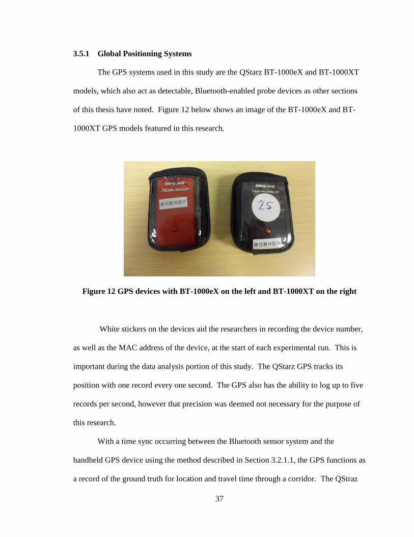
37
3.5.1 Global Positioning Systems
The GPS systems used in this study are the QStarz BT-1000eX and BT-1000XT
models, which also act as detectable, Bluetooth-enabled probe devices as other sections
of this thesis have noted. Figure 12 below shows an image of the BT-1000eX and BT-
1000XT GPS models featured in this research.
Figure 12 GPS devices with BT-1000eX on the left and BT-1000XT on the right
White stickers on the devices aid the researchers in recording the device number,
as well as the MAC address of the device, at the start of each experimental run. This is
important during the data analysis portion of this study. The QStarz GPS tracks its
position with one record every one second. The GPS also has the ability to log up to five
records per second, however that precision was deemed not necessary for the purpose of
this research.
With a time sync occurring between the Bluetooth sensor system and the
handheld GPS device using the method described in Section 3.2.1.1, the GPS functions as
a record of the ground truth for location and travel time through a corridor. The QStraz

38
GPS data is transferred to the computer via a USB connection using the QTravel software
package. Figure 13 shows a screenshot of the QTravel software with the data logged by
the GPS.
Figure 13 Screenshot of QTravel Software
The QTravel software also allows the user to insert a point, to which the program
assigns geographic coordinates. This became helpful when inserting the location of the
Bluetooth sensor stations along deployment routes to calculate the position offset of the
device at the point of detection. The raw GPS data collected during the deployments can
be exported to a comma separated value (.csv) file type which can then be converted to a
Microsoft Excel file for processing. Information captured in the raw data file includes
the date, timestamp, latitudinal and longitudinal coordinates, device speed, altitude, etc.

39
3.5.2 Video Cameras
Video cameras can also provide a way to collect ground truth travel time data
when collecting Bluetooth travel time. The video cameras used during the data collection
efforts are Panasonic HDC-TM700 video cameras mounted on tripods. Video cameras
become an efficient ground truth data collection method when the corridor is so long that
a probe vehicle would not be able to complete a sufficient number of passes through the
system. The object of analysis for video ground truth data is matching the license plate
detection at each site. By performing a time-sync between the video cameras and the
Bluetooth system again using the process outlined in Section 3.2.1.1, the time stamps and
extrapolated travel time from license plate records become a ground truth measure to
compare to Bluetooth travel time. However, a drawback of this method is that the
license plate data must be manually recorded from the video requiring a potential
significant additional data collection effort after field data collection.
For the given study sections freeway data collection captures the morning traffic
peak, where the travel time of a probe vehicle loop is upwards of 30 minutes. This is
impractical because only four to five runs could be achieved during the deployment
period, which is insufficient to provide a significant ground truth record. The video
cameras are placed on the overpasses facing the rear of the passing vehicles to capture
their license plates. The cameras must be focused through the chain-link fence present at
most overpasses, so that there is no obstruction of license plates during the processing of
the video. The camera view is such that each camera focuses on two lanes of traffic, with
the edges of the lanes hitting the middle of the video camera view. Figure 14 below
shows the typical configuration of the overpass video cameras.
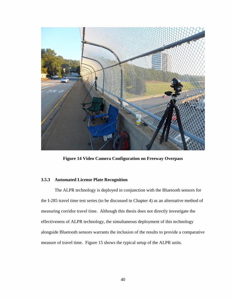
40
Figure 14 Video Camera Configuration on Freeway Overpass
3.5.3 Automated License Plate Recognition
The ALPR technology is deployed in conjunction with the Bluetooth sensors for
the I-285 travel time test series (to be discussed in Chapter 4) as an alternative method of
measuring corridor travel time. Although this thesis does not directly investigate the
effectiveness of ALPR technology, the simultaneous deployment of this technology
alongside Bluetooth sensors warrants the inclusion of the results to provide a comparative
measure of travel time. Figure 15 shows the typical setup of the ALPR units.
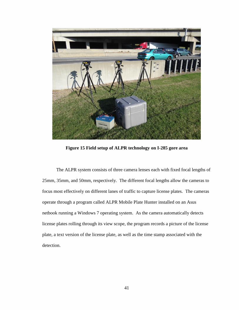
41
Figure 15 Field setup of ALPR technology on I-285 gore area
The ALPR system consists of three camera lenses each with fixed focal lengths of
25mm, 35mm, and 50mm, respectively. The different focal lengths allow the cameras to
focus most effectively on different lanes of traffic to capture license plates. The cameras
operate through a program called ALPR Mobile Plate Hunter installed on an Asus
netbook running a Windows 7 operating system. As the camera automatically detects
license plates rolling through its view scope, the program records a picture of the license
plate, a text version of the license plate, as well as the time stamp associated with the
detection.

42
Chapter 4: Experimental Design
4.1 Introduction
There are two components the research team investigated to provide guidance on
how best to increase the accuracy of real-time travel time measurement in a work zone
corridor. The first is developing a method to maximize the number of Bluetooth-enabled
devices the Bluetooth sensor can detect with the understanding that the confidence
bounds surrounding the travel time will thus decrease; and the second is optimizing the
frequency of sensor placement along a corridor to account for the inherent error in
detection location around a sensor and the resultant error in travel time.
To investigate how the sample size of Bluetooth sensor detection can be
increased, it is important to first explore factors that influence the number of devices the
sensor can detect. These factors include characteristics of the device, such as the pattern
of detection, which influences the likelihood of detection; and the characteristics of the
sensor, such as the sensor capacity for detection. This thesis seeks to explore these
questions by investigating the device and sensor characteristics so that the most effective
method of Bluetooth device detection can be employed. Because of the innate
differences in Bluetooth devices present in the detectable population, this thesis
investigates the detection properties of different device groups independently, as well as
jointly, and observes the effect as more and different devices are brought into a sensor’s
field of view.
Secondly, sensor placement frequency refers to the spacing or separation of
Bluetooth sensors along a travel-way. When a Bluetooth-enabled device is detected by a
43
Bluetooth sensor, there is a location range around the sensor from where the detection
originated. Knowing this spread of detection location around a sensor is important when
spacing the sensors to calculating the resulting error in speed and travel time derivation.
4.2 Bluetooth Device and Sensor Characteristics
To explore device and sensor properties the research team performed a series of
tests in a controlled indoor environment in one of the lab rooms at the Georgia Institute of
Technology. There was minimal noise/interference from other devices other than those
tested, and the research team was able to bring a controlled group of devices into a
sensors field of view for pre-determined lengths of time to observe the behavior of both
the sensor and Class 1 and Class 2 devices. The research team used a combination of the
Class 1 and Class 2 devices presented in Section 3.1. The two tests conducted include a
single-sensor capacity test, and a multiple sensor effect test. The following sections of
this thesis describe the details of the sensor and device test series.
4.2.1 Test Series 1: Single-Sensor Capacity
4.2.1.1 Overview
Sensor capacity represents the maximum number of Bluetooth-enabled devices
that a Bluetooth sensor can detect during an 11.24 second cycle. The research team
designed a controlled test to investigate the number of devices that a Class 1 Bluetooth
sensor can detect during an 11.24 second cycle by bringing an increasing number of
devices into the sensors field of view (by turning additional devices on in a controlled
manner), and looking for a point where the detection rate begins to drop off. The
research also focused on providing a distinction between Class 1 and Class 2 devices to
44
see if the sensor has a higher propensity for detection based on Bluetooth power class.
The sensor used for the Single Sensor Capacity test series is Sensor 5.
4.2.1.2 Day 1: Single-Sensor and Class 2 Devices
The first day of the single-sensor capacity test series involved testing a series of
5,10,15,20, and 25 Class 2 devices, each for a ten minute period (equating to about 53
11.24 second cycles). The 25 Class 2 devices were a combination of 15 QStarz BT-
1000eX devices (Number 6 through 20, in the following tables) and ten QStarz BT-
1000XT devices (Number 21 through 30). All devices were placed on a conference table
in rows of five devices, with about six inches of separation between each device (Figure
16). The first five devices in the closest row to the sensor were turned to the on position
for the first ten minutes. Then, without the first five devices being turned off, the next
five devices were turned on for the following ten minute period. The Class 2 test
proceeded in this manner until all 25 devices were turned on at once. Figure 16 shows a
view of the deployment configuration containing 20 devices. The final deployment
configuration contained one more row of GPS units on the further side away from the
sensor, following the same spacing arrangement as the first 20 devices. Figure 16 also
shows the location of the Class 1 Bluetooth sensor. The sensor is at a height of
approximately eight feet, and is offset horizontally by about five feet from the closest row
of GPS devices.
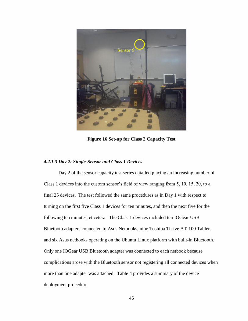
45
Figure 16 Set-up for Class 2 Capacity Test
4.2.1.3 Day 2: Single-Sensor and Class 1 Devices
Day 2 of the sensor capacity test series entailed placing an increasing number of
Class 1 devices into the custom sensor’s field of view ranging from 5, 10, 15, 20, to a
final 25 devices. The test followed the same procedures as in Day 1 with respect to
turning on the first five Class 1 devices for ten minutes, and then the next five for the
following ten minutes, et cetera. The Class 1 devices included ten IOGear USB
Bluetooth adapters connected to Asus Netbooks, nine Toshiba Thrive AT-100 Tablets,
and six Asus netbooks operating on the Ubuntu Linux platform with built-in Bluetooth.
Only one IOGear USB Bluetooth adapter was connected to each netbook because
complications arose with the Bluetooth sensor not registering all connected devices when
more than one adapter was attached. Table 4 provides a summary of the device
deployment procedure.
Sensor 5
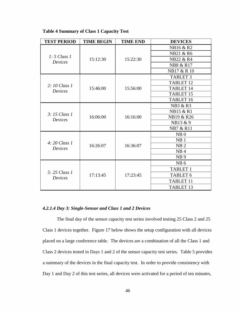
46
Table 4 Summary of Class 1 Capacity Test
TEST PERIOD TIME BEGIN TIME END DEVICES
1: 5 Class 1
Devices 15:12:30 15:22:30
NB16 & R2 NB21 & R6 NB22 & R4 NB8 & R17
NB17 & R 10
2: 10 Class 1
Devices 15:46:00 15:56:00
TABLET 3 TABLET 12 TABLET 14 TABLET 15 TABLET 16
3: 15 Class 1
Devices 16:06:00 16:16:00
NB3 & R3 NB15 & R1 NB19 & R26
NB13 & 9 NB7 & R11
4: 20 Class 1
Devices 16:26:07 16:36:07
NB 0 NB 1 NB 2 NB 4 NB 9
5: 25 Class 1
Devices 17:13:45 17:23:45
NB 6 TABLET 1 TABLET 6 TABLET 11 TABLET 13
4.2.1.4 Day 3: Single-Sensor and Class 1 and 2 Devices
The final day of the sensor capacity test series involved testing 25 Class 2 and 25
Class 1 devices together. Figure 17 below shows the setup configuration with all devices
placed on a large conference table. The devices are a combination of all the Class 1 and
Class 2 devices tested in Days 1 and 2 of the sensor capacity test series. Table 5 provides
a summary of the devices in the final capacity test. In order to provide consistency with
Day 1 and Day 2 of this test series, all devices were activated for a period of ten minutes,

47
or about 53 complete detection cycles. A separation of approximately six inches was
maintained between each device for the entire deployment series to avoid direction
interference between Bluetooth antennae.
Table 5 Bluetooth-Enabled Devices in Final Sensor Capacity Test
Power Class Count
IOGear USB Bluetooth Adapter Class 1 10
Asus Eee PC Netbook
Class 1 6
Toshiba Thrive AT-100 Tablet Class 1 9
QStarz BT-1000eX Class 2 15
QStarz BT-1000XT
Class 2 10
TOTAL 50
Figure 17 Class 1 and 2 device configuration for sensor capacity final test
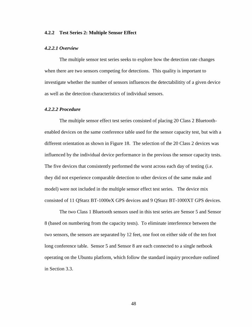
48
4.2.2 Test Series 2: Multiple Sensor Effect
4.2.2.1 Overview
The multiple sensor test series seeks to explore how the detection rate changes
when there are two sensors competing for detections. This quality is important to
investigate whether the number of sensors influences the detectabilitity of a given device
as well as the detection characteristics of individual sensors.
4.2.2.2 Procedure
The multiple sensor effect test series consisted of placing 20 Class 2 Bluetooth-
enabled devices on the same conference table used for the sensor capacity test, but with a
different orientation as shown in Figure 18. The selection of the 20 Class 2 devices was
influenced by the individual device performance in the previous the sensor capacity tests.
The five devices that consistently performed the worst across each day of testing (i.e.
they did not experience comparable detection to other devices of the same make and
model) were not included in the multiple sensor effect test series. The device mix
consisted of 11 QStarz BT-1000eX GPS devices and 9 QStarz BT-1000XT GPS devices.
The two Class 1 Bluetooth sensors used in this test series are Sensor 5 and Sensor
8 (based on numbering from the capacity tests). To eliminate interference between the
two sensors, the sensors are separated by 12 feet, one foot on either side of the ten foot
long conference table. Sensor 5 and Sensor 8 are each connected to a single netbook
operating on the Ubuntu platform, which follow the standard inquiry procedure outlined
in Section 3.3.
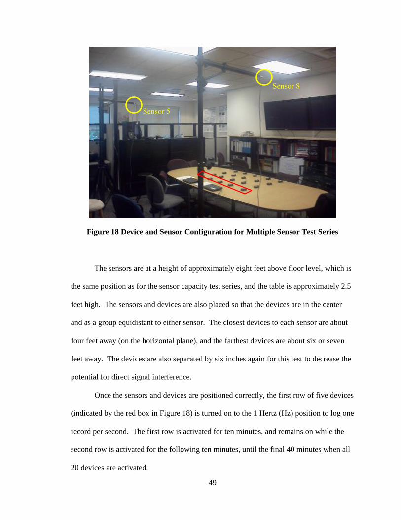
49
Figure 18 Device and Sensor Configuration for Multiple Sensor Test Series
The sensors are at a height of approximately eight feet above floor level, which is
the same position as for the sensor capacity test series, and the table is approximately 2.5
feet high. The sensors and devices are also placed so that the devices are in the center
and as a group equidistant to either sensor. The closest devices to each sensor are about
four feet away (on the horizontal plane), and the farthest devices are about six or seven
feet away. The devices are also separated by six inches again for this test to decrease the
potential for direct signal interference.
Once the sensors and devices are positioned correctly, the first row of five devices
(indicated by the red box in Figure 18) is turned on to the 1 Hertz (Hz) position to log one
record per second. The first row is activated for ten minutes, and remains on while the
second row is activated for the following ten minutes, until the final 40 minutes when all
20 devices are activated.
Sensor 5
Sensor 8

50
4.3 Investigation of Detection Range
4.3.1 Objective
The focus of the detection range deployment is to capture the position of Class 1
and Class 2 Bluetooth-enabled devices when they are detected by a Class 1 Bluetooth
sensor as they travel through a corridor. The additional purpose of this test is to assess
whether the most accurate travel time calculation uses a first-to-first detection pairing, a
last-to-last detection pairing, or a combination of the two (i.e. a centroid). The
assumption going into this test is that Class 1 devices will experience a larger range of
detection location than will the Class 2 devices, due to Class 1 devices being of a higher
power class and having the ability to communicate over roughly three times the distance
as Class 2 devices.
4.3.2 Deployment Location
The research team found it important to test the device detection range on a
corridor containing both a midblock location (no signal, with a stop bar on the side
street), and an intersection location (with a signal). The reasoning behind this view is
that an intersection location is indicative of a stop-and-go work zone corridor, where
traffic must stop or move slowly because of a delay for several seconds and then resume
free-flow. The midblock location represents the scenario of consistent flow through the
system, where very rare stop and slowed conditions occur.
An additional consideration to site identification was the selection of a corridor
where free flow speed was a slow speed (around 30 mph), so the research team could
capture conditions more representative of an active work zone. Furthermore, the research
team wanted to incorporate probe vehicles containing Class 1 and Class 2 Bluetooth-
51
enabled devices, so selecting a location that allows for quick vehicle turn-around was
important. The site that met these conditions, and was also within a reasonable driving
distance from the group research lab, is 14th
Street, west of the I-75/85 downtown
connector. Figure 19 below shows an aerial view of the corridor, with the Bluetooth
sensor locations denoted by a yellow triangle, and the turnaround (TA) locations denoted
by a red circle and labeled TA 1 and TA 2.
Figure 19 Aerial view of 14th
Street Deployment Corridor
The Bluetooth sensors were placed on the right side of the eastbound traffic.
Each site features one custom Bluetooth sensor, and one Digiwest Bluetooth sensor,
configured using the method described in Section 3.2. Site A is the midblock location at
the intersection of 14th
Street and Center Street (on the east corner of the intersection),
and Site B is the intersection location at the crossing of 14th
Street and State Street (at the
west corner of the intersection). TA 1 and TA 2 were the turnaround locations. Table 6
provides the geographic coordinates for each sensor station and turnaround location.
TA1 TA2
Turnaround
(TA) Location
Legend
Bluetooth Sensor
Location
Midblock Intersection
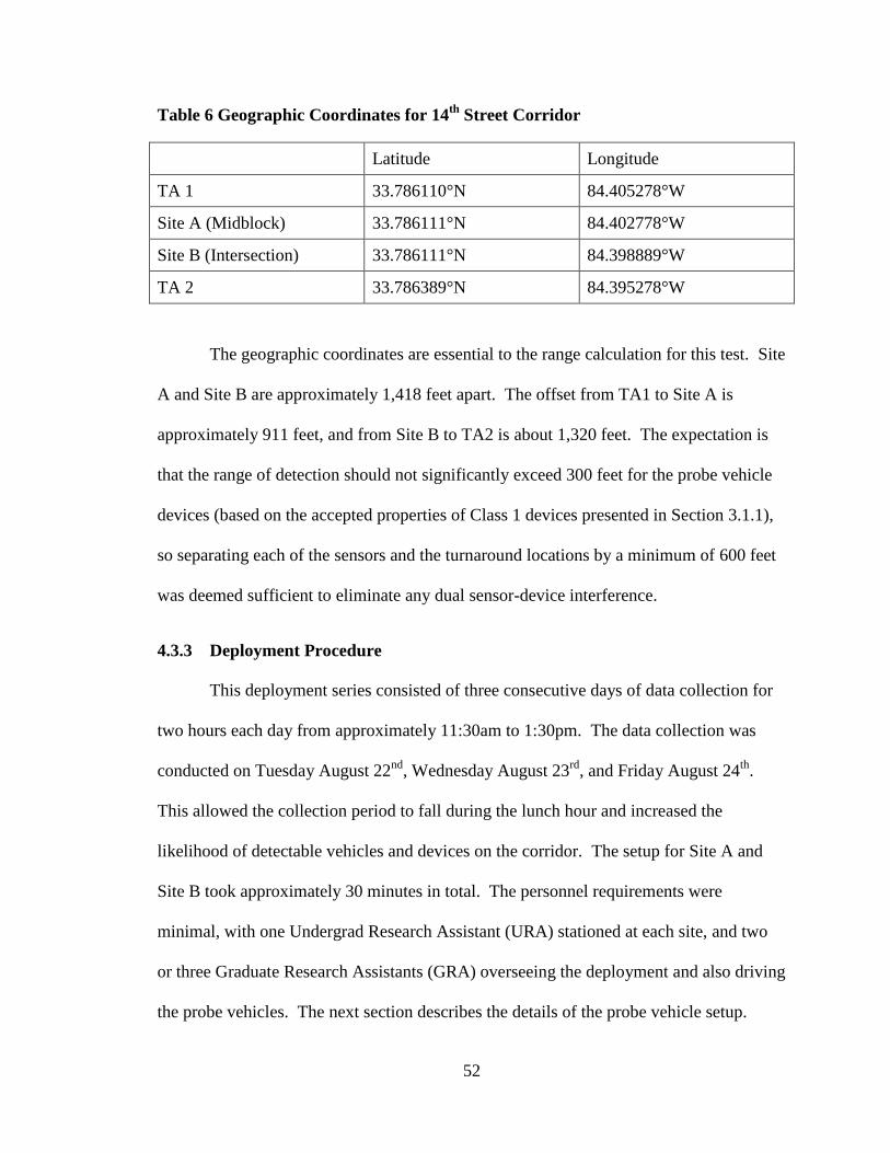
52
Table 6 Geographic Coordinates for 14th
Street Corridor
Latitude Longitude
TA 1 33.786110°N 84.405278°W
Site A (Midblock) 33.786111°N 84.402778°W
Site B (Intersection) 33.786111°N 84.398889°W
TA 2 33.786389°N 84.395278°W
The geographic coordinates are essential to the range calculation for this test. Site
A and Site B are approximately 1,418 feet apart. The offset from TA1 to Site A is
approximately 911 feet, and from Site B to TA2 is about 1,320 feet. The expectation is
that the range of detection should not significantly exceed 300 feet for the probe vehicle
devices (based on the accepted properties of Class 1 devices presented in Section 3.1.1),
so separating each of the sensors and the turnaround locations by a minimum of 600 feet
was deemed sufficient to eliminate any dual sensor-device interference.
4.3.3 Deployment Procedure
This deployment series consisted of three consecutive days of data collection for
two hours each day from approximately 11:30am to 1:30pm. The data collection was
conducted on Tuesday August 22nd
, Wednesday August 23rd
, and Friday August 24th
.
This allowed the collection period to fall during the lunch hour and increased the
likelihood of detectable vehicles and devices on the corridor. The setup for Site A and
Site B took approximately 30 minutes in total. The personnel requirements were
minimal, with one Undergrad Research Assistant (URA) stationed at each site, and two
or three Graduate Research Assistants (GRA) overseeing the deployment and also driving
the probe vehicles. The next section describes the details of the probe vehicle setup.
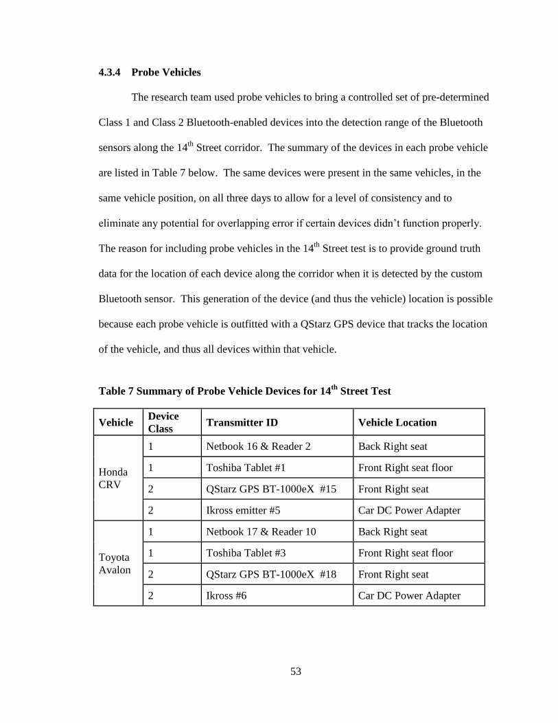
53
4.3.4 Probe Vehicles
The research team used probe vehicles to bring a controlled set of pre-determined
Class 1 and Class 2 Bluetooth-enabled devices into the detection range of the Bluetooth
sensors along the 14th
Street corridor. The summary of the devices in each probe vehicle
are listed in Table 7 below. The same devices were present in the same vehicles, in the
same vehicle position, on all three days to allow for a level of consistency and to
eliminate any potential for overlapping error if certain devices didn’t function properly.
The reason for including probe vehicles in the 14th
Street test is to provide ground truth
data for the location of each device along the corridor when it is detected by the custom
Bluetooth sensor. This generation of the device (and thus the vehicle) location is possible
because each probe vehicle is outfitted with a QStarz GPS device that tracks the location
of the vehicle, and thus all devices within that vehicle.
Table 7 Summary of Probe Vehicle Devices for 14th
Street Test
Vehicle Device
Class Transmitter ID Vehicle Location
Honda
CRV
1 Netbook 16 & Reader 2 Back Right seat
1 Toshiba Tablet #1 Front Right seat floor
2 QStarz GPS BT-1000eX #15 Front Right seat
2 Ikross emitter #5 Car DC Power Adapter
Toyota
Avalon
1 Netbook 17 & Reader 10 Back Right seat
1 Toshiba Tablet #3 Front Right seat floor
2 QStarz GPS BT-1000eX #18 Front Right seat
2 Ikross #6 Car DC Power Adapter
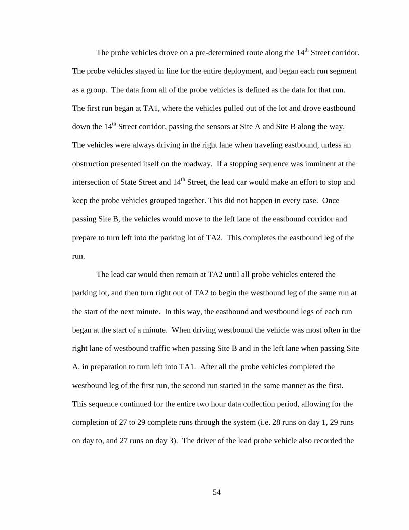
54
The probe vehicles drove on a pre-determined route along the 14th
Street corridor.
The probe vehicles stayed in line for the entire deployment, and began each run segment
as a group. The data from all of the probe vehicles is defined as the data for that run.
The first run began at TA1, where the vehicles pulled out of the lot and drove eastbound
down the 14th
Street corridor, passing the sensors at Site A and Site B along the way.
The vehicles were always driving in the right lane when traveling eastbound, unless an
obstruction presented itself on the roadway. If a stopping sequence was imminent at the
intersection of State Street and 14th
Street, the lead car would make an effort to stop and
keep the probe vehicles grouped together. This did not happen in every case. Once
passing Site B, the vehicles would move to the left lane of the eastbound corridor and
prepare to turn left into the parking lot of TA2. This completes the eastbound leg of the
run.
The lead car would then remain at TA2 until all probe vehicles entered the
parking lot, and then turn right out of TA2 to begin the westbound leg of the same run at
the start of the next minute. In this way, the eastbound and westbound legs of each run
began at the start of a minute. When driving westbound the vehicle was most often in the
right lane of westbound traffic when passing Site B and in the left lane when passing Site
A, in preparation to turn left into TA1. After all the probe vehicles completed the
westbound leg of the first run, the second run started in the same manner as the first.
This sequence continued for the entire two hour data collection period, allowing for the
completion of 27 to 29 complete runs through the system (i.e. 28 runs on day 1, 29 runs
on day to, and 27 runs on day 3). The driver of the lead probe vehicle also recorded the

55
time when each eastbound/westbound leg of each run began, for reference during the data
processing.
4.4 Freeway Side-Fire Travel Time
4.4.1 Objective
The objective of the freeway side-fire test is to apply the lessons learned in the
Sensor and Device Characteristics tests and the Detection Range test to measuring real-
time travel time. The research team chose to position the Bluetooth sensors in side-fire
mode because this is most available and accessible position along a typical work zone
corridor, and does not require the construction of additional mounting mechanisms
needed for overhead positioning. An additional focus of this test is comparing the
detectability of devices traveling in the direction adjacent to the Bluetooth sensor to those
traveling in the opposite direction with greater sensor separation, and cultivating an
understanding for the different detection rates of the two groups.
4.4.2 Deployment Location
The research team selected a section of the I-285 eastbound corridor around
Atlanta ten miles in length, from Paces Ferry Road to Ashford Dunwoody Road, as the
location for the freeway side-fire travel time test series. The research team selected this
corridor because it was an active work zone on the weekends (with partial lane closures
along corridor), and an inactive work zone on the weekdays (with all lanes open). This
travel time test series featured weekday deployments in the non-active work zone in
preparation for the following test series, which consists of travel time measurement in an
active work zone. By deploying several times along the I-285 corridor, the research

56
team was able to become familiar with the test sites, as well as generate a control dataset
for the active work zone travel times.
4.4.2.1 Site Selection Process
There were several considerations that were accounted for when selecting the
sites for Bluetooth deployment along the I-285 corridor. First, the Bluetooth sites
selected should minimize interference from surrounding objects and devices. Examples
of object interference include vegetation cover and obstructing wall, signs, and fences.
Proximity to stationary or nearby corridors can lead to the detection of unwanted
Bluetooth-enabled devices that can complicate the travel time calculation, or reduce the
number of unique detections of strictly corridor devices. Therefore, selecting sites that
would minimize interference is important.
The accessibility of the site location is also important so that the equipment can be
safely and easily transported, setup, and broken down. Therefore, the sites must be
accessible via a sidewalk and crosswalk from a nearby parking area, or have a wide
protected shoulder adequate for temporarily parking a vehicle to unload equipment. The
temporary vehicle pull-off is only considered safe when in the gore area of a freeway
overpass where passing vehicles are entering or exiting the corridor at slower speeds.
The site must also have level ground to support the Bluetooth tripod configuration, and
feature a wall or guardrail to protect the personnel and equipment. The constraints were
generally imposed for the safety of the data collection team, who were not part of the
construction site personnel. Future efforts could employ and instrumented work zone
truck. It is anticipated that when deployed by a contractor additional sites would be
available that were not considered in this effort.

57
Another important consideration for site selection is the availability of an
overpass to place cameras to capture license plates of passing vehicles along the corridor.
The cameras are necessary to the study because they provide the method of ground truth
travel time data collection. Finally, because the purpose of this data collection is to
collection travel times, selecting work zone segments not including a major interchange
was desirable to maximize the likelihood of vehicles traversing the entire work zone.
Otherwise, a great portion of the vehicles traveling between two points may exit at a
major interchange and not generate travel time measurements.
Although all of these considerations are important when selection the optimal
locations to station the Bluetooth sensors, the consideration of safety and accessibility are
of greatest importance in this research effort. This puts the site location options at
freeway interchanges in the gore area of an overpass where there is protection behind a
wall or a guardrail. The gore area between the freeway exit ramp is most ideal, because
even if a device is detected exiting the freeway, the assumption is that the vehicle will not
be directly re-entering the freeway, and thus will not provide a significant measure of
error in the travel time.
4.4.2.2 Site Identification
The research team identified three feasible sites for data collection on the
eastbound section of the I-285 corridor to use for measuring eastbound morning peak
corridor travel times. One custom Bluetooth sensor was stationed at each site and one
ALPR system was also stationed at two sites on each day of deployment. Figure 20
below shows an aerial view of the deployment corridor for the freeway side-fire travel
time measure.

58
Figure 20 Aerial View of I-285 Eastbound Deployment Locations
Site A is located at the intersection of I-285 and Paces Ferry Road, Site B is
located at the intersection of I-285 and Northside Drive, and Site C is located at the
intersection of I-285 and Roswell Road. The location of Ashford Dunwoody Road is also
shown on the corridor for spatial reference. Paces Ferry Road is shown with a red box to
highlight that it is at the end of the work zone corridor, and also the first eastbound
corridor location. The distance between Paces Ferry Road and Northside Drive is
approximately 4.3 miles, and between Northside Drive and Roswell Road is
approximately 3.3 miles. Figure 21, Figure 22, and Figure 23 show aerial views of the
Paces Ferry Road, Northside Drive, and Roswell Road sites, respectively. The Paces
Ferry Road site is approximately 175 feet from the overpass, the Northside Drive site is
approximately 175 feet, and the Roswell Road site is about 150 feet from the overpass.
Paces
Ferry Road
Northside
Drive
Roswell
Road
Ashford
Dunwoody Road
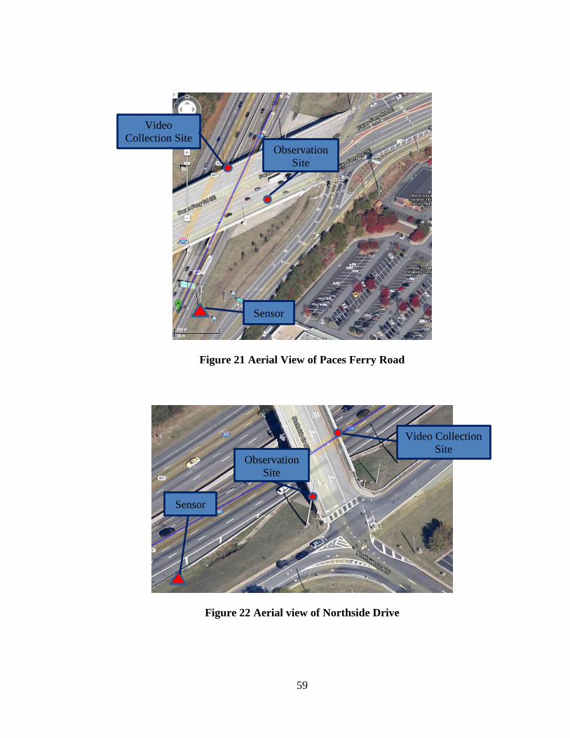
59
Figure 21 Aerial View of Paces Ferry Road
Figure 22 Aerial view of Northside Drive
Sensor
Observation
Site
Video
Collection Site
Observation
Site
Sensor
Video Collection
Site

60
Figure 23 Aerial View of Roswell Road
4.4.3 Deployment Procedure
Before every data collection field deployment, the research team provided a plan
to the Georgia Department of Transportation (GDOT), which in all cases had to be
approved before collection began. Furthermore, the research team contacted the local
law enforcement personnel for each data collection site to advise them of the location,
duration, and equipment that would be present for the data collection.
4.4.3.1 Day 1: Friday, September 7th
, 2012
For the first day of data collection, the research team deployed to two sites, Paces
Ferry Road and Northside Drive. There were two data collection teams at each site, each
with three URAs and one GRA. The Bluetooth sensors were assembled at both sites by
8:05 AM. The planned end of data collection for Paces Ferry Road was 10:25 AM, and
Observation
Site
Sensor
Video Collection
Site
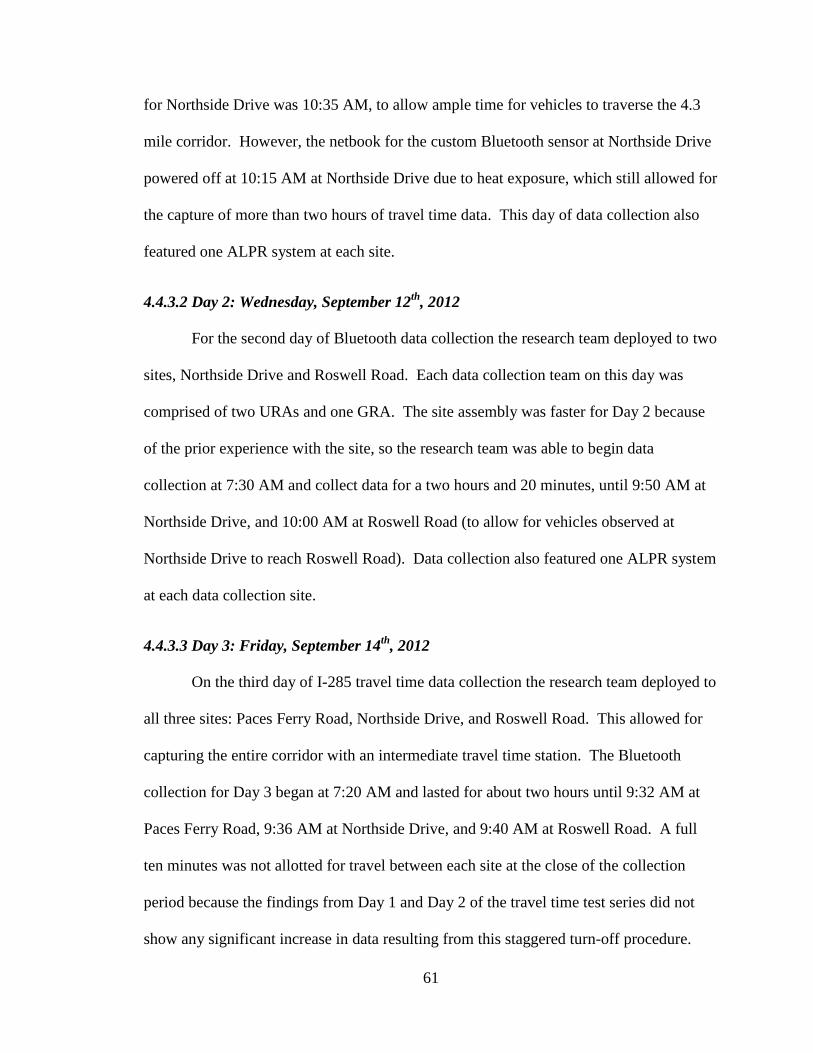
61
for Northside Drive was 10:35 AM, to allow ample time for vehicles to traverse the 4.3
mile corridor. However, the netbook for the custom Bluetooth sensor at Northside Drive
powered off at 10:15 AM at Northside Drive due to heat exposure, which still allowed for
the capture of more than two hours of travel time data. This day of data collection also
featured one ALPR system at each site.
4.4.3.2 Day 2: Wednesday, September 12th
, 2012
For the second day of Bluetooth data collection the research team deployed to two
sites, Northside Drive and Roswell Road. Each data collection team on this day was
comprised of two URAs and one GRA. The site assembly was faster for Day 2 because
of the prior experience with the site, so the research team was able to begin data
collection at 7:30 AM and collect data for a two hours and 20 minutes, until 9:50 AM at
Northside Drive, and 10:00 AM at Roswell Road (to allow for vehicles observed at
Northside Drive to reach Roswell Road). Data collection also featured one ALPR system
at each data collection site.
4.4.3.3 Day 3: Friday, September 14th
, 2012
On the third day of I-285 travel time data collection the research team deployed to
all three sites: Paces Ferry Road, Northside Drive, and Roswell Road. This allowed for
capturing the entire corridor with an intermediate travel time station. The Bluetooth
collection for Day 3 began at 7:20 AM and lasted for about two hours until 9:32 AM at
Paces Ferry Road, 9:36 AM at Northside Drive, and 9:40 AM at Roswell Road. A full
ten minutes was not allotted for travel between each site at the close of the collection
period because the findings from Day 1 and Day 2 of the travel time test series did not
show any significant increase in data resulting from this staggered turn-off procedure.

62
On this third day of data collection Bluetooth sensors were placed at all three data
collection sites, and ALPR systems were stationed at Northside Drive and Roswell Road.
These two sites were used to maximize the potential for plate matches as any site pair
containing Paces Ferry Road tended to lose significant number of potential matches due
to the I-75/I-285 interchange.
4.4.4 Ground Truth
Given the route length, and the potential for a 30-minute driving loop for the
probe vehicles, it was determined that probe vehicles data would not provide a sufficient
travel time sample for the freeway studies. Therefore, the method of ground truth for the
I-285 data collection series is license plate matching, as described in Section 3.5.2. Paces
Ferry Road has four lanes of eastbound traffic, so two video cameras were necessary for
this site. Northside Drive and Roswell Road each have five lanes of eastbound traffic, so
three video cameras were necessary to capture no more than two lanes of traffic a piece.
(Previous efforts under different projects conducted at Georgia Institute of Technology
have shown limiting video capture to two lanes per camera allows for optimal manual
license plate data collection [42].) Section 5.5.2 of this thesis summarizes the processing
method for matching license plates captured by the overpass video cameras.
4.5 Work Zone Travel Time
4.5.1 Objective
The objective of the work zone travel time test is to assess the effectiveness of
using Bluetooth to measure travel time through an active work zone corridor. The
research team again placed the Bluetooth sensors in side-fire locations, comparable to the
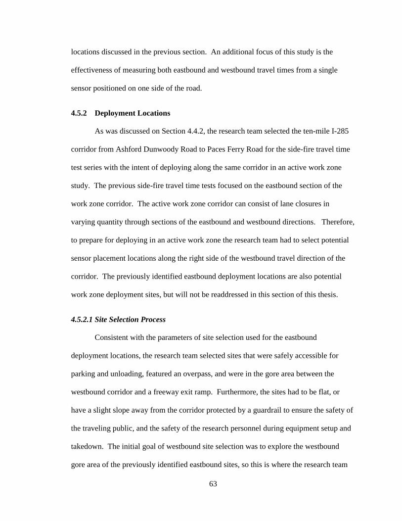
63
locations discussed in the previous section. An additional focus of this study is the
effectiveness of measuring both eastbound and westbound travel times from a single
sensor positioned on one side of the road.
4.5.2 Deployment Locations
As was discussed on Section 4.4.2, the research team selected the ten-mile I-285
corridor from Ashford Dunwoody Road to Paces Ferry Road for the side-fire travel time
test series with the intent of deploying along the same corridor in an active work zone
study. The previous side-fire travel time tests focused on the eastbound section of the
work zone corridor. The active work zone corridor can consist of lane closures in
varying quantity through sections of the eastbound and westbound directions. Therefore,
to prepare for deploying in an active work zone the research team had to select potential
sensor placement locations along the right side of the westbound travel direction of the
corridor. The previously identified eastbound deployment locations are also potential
work zone deployment sites, but will not be readdressed in this section of this thesis.
4.5.2.1 Site Selection Process
Consistent with the parameters of site selection used for the eastbound
deployment locations, the research team selected sites that were safely accessible for
parking and unloading, featured an overpass, and were in the gore area between the
westbound corridor and a freeway exit ramp. Furthermore, the sites had to be flat, or
have a slight slope away from the corridor protected by a guardrail to ensure the safety of
the traveling public, and the safety of the research personnel during equipment setup and
takedown. The initial goal of westbound site selection was to explore the westbound
gore area of the previously identified eastbound sites, so this is where the research team

64
began the investigation. The process of site selection involved completing an initial
search of the corridor area using Google Maps, and then driving along the corridor to
visit and catalogue the potential sites.
4.5.2.2 Site Identification
The research team found two potential sites in the westbound direction along the
ten mile work zone corridor, shown in green in Figure 24 below. Figure 24 also
identifies the three eastbound data collection sites, shown in blue. The ends of the work
zone corridor are indicated with boxes outlined in red.
Figure 24 Aerial View of I-285 Westbound Deployment Locations
One custom Bluetooth sensor was stationed at each site during the work zone
deployment and one ALPR system was at two sites on each day of deployment. The first
westbound site is Riverside Drive, and the second is Paces Ferry Road, separated by a
Paces Ferry
Road
Northside
Drive
Roswell
Road
Ashford
Dunwoody Road
Riverside
Drive
Paces Ferry
Road

65
distance of 5.9 miles, and divided by I-75, a place for major ingress/egress of vehicles
and thus potential loss of many travel time pairs. Figure 25 and Figure 26 below show
aerial views of the Riverside Drive and Paces Ferry Road data collection sites. The Paces
Ferry Road site is approximately 75 feet from the overpass, and Riverside Drive is about
150 feet from the overpass.
Figure 25 Aerial view of Riverside Drive
Observation
Site
Sensor
Video Collection
Site

66
Figure 26 Aerial view of Paces Ferry Road Westbound
4.5.3 Deployment Procedure
The deployment procedure for the work zone travel time test series was dependent
on the weekend lane closure plan for the active I-285 work zone. The construction plan
for an upcoming weekend was not released until the Wednesday before the weekend
closure. This reporting schedule required the research team to contact GDOT about the
upcoming lane closures on a weekly basis, to construct a plan for deployment
accordingly, and assess whether the given lane closures were consistent with the
deployment capabilities of the Bluetooth (and the jointly deployed ALPR technology).
All work zone data collection plans were approved by GDOT, and the research team
notified the local law enforcement personnel of the planned activities prior to each
deployment session.
Observation
Site
Sensor
Video Collection
Site
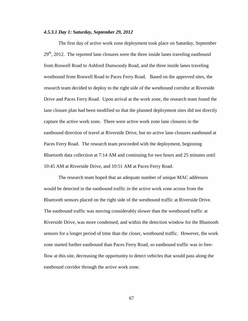
67
4.5.3.1 Day 1: Saturday, September 29, 2012
The first day of active work zone deployment took place on Saturday, September
29th
, 2012. The reported lane closures were the three inside lanes traveling eastbound
from Roswell Road to Ashford Dunwoody Road, and the three inside lanes traveling
westbound from Roswell Road to Paces Ferry Road. Based on the approved sites, the
research team decided to deploy to the right side of the westbound corridor at Riverside
Drive and Paces Ferry Road. Upon arrival at the work zone, the research team found the
lane closure plan had been modified so that the planned deployment sites did not directly
capture the active work zone. There were active work zone lane closures in the
eastbound direction of travel at Riverside Drive, but no active lane closures eastbound at
Paces Ferry Road. The research team proceeded with the deployment, beginning
Bluetooth data collection at 7:14 AM and continuing for two hours and 25 minutes until
10:45 AM at Riverside Drive, and 10:51 AM at Paces Ferry Road.
The research team hoped that an adequate number of unique MAC addresses
would be detected in the eastbound traffic in the active work zone across from the
Bluetooth sensors placed on the right side of the westbound traffic at Riverside Drive.
The eastbound traffic was moving considerably slower than the westbound traffic at
Riverside Drive, was more condensed, and within the detection window for the Bluetooth
sensors for a longer period of time than the closer, westbound traffic. However, the work
zone started further eastbound than Paces Ferry Road, so eastbound traffic was in free-
flow at this site, decreasing the opportunity to detect vehicles that would pass along the
eastbound corridor through the active work zone.
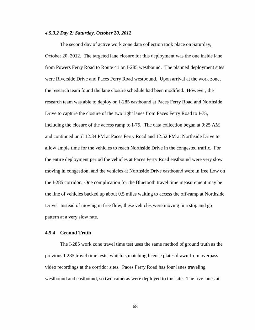
68
4.5.3.2 Day 2: Saturday, October 20, 2012
The second day of active work zone data collection took place on Saturday,
October 20, 2012. The targeted lane closure for this deployment was the one inside lane
from Powers Ferry Road to Route 41 on I-285 westbound. The planned deployment sites
were Riverside Drive and Paces Ferry Road westbound. Upon arrival at the work zone,
the research team found the lane closure schedule had been modified. However, the
research team was able to deploy on I-285 eastbound at Paces Ferry Road and Northside
Drive to capture the closure of the two right lanes from Paces Ferry Road to I-75,
including the closure of the access ramp to I-75. The data collection began at 9:25 AM
and continued until 12:34 PM at Paces Ferry Road and 12:52 PM at Northside Drive to
allow ample time for the vehicles to reach Northside Drive in the congested traffic. For
the entire deployment period the vehicles at Paces Ferry Road eastbound were very slow
moving in congestion, and the vehicles at Northside Drive eastbound were in free flow on
the I-285 corridor. One complication for the Bluetooth travel time measurement may be
the line of vehicles backed up about 0.5 miles waiting to access the off-ramp at Northside
Drive. Instead of moving in free flow, these vehicles were moving in a stop and go
pattern at a very slow rate.
4.5.4 Ground Truth
The I-285 work zone travel time test uses the same method of ground truth as the
previous I-285 travel time tests, which is matching license plates drawn from overpass
video recordings at the corridor sites. Paces Ferry Road has four lanes traveling
westbound and eastbound, so two cameras were deployed to this site. The five lanes at

69
Riverside Drive and Northside Drive required the deployment of three overpass video
cameras.

70
Chapter 5: Data Processing and Analysis Parameters
5.1 Introduction
The procedure for data processing and analysis is an important consideration of
this thesis. Of main importance is discussing the parameters that were used in the data
analysis to provide relevance to the results presented in Chapter 6. This Chapter provides
a description of the device and sensor characteristics that are a focal point in the analysis
of different device/sensor test configurations. This Chapter also discusses the method of
calculating the device detection range, and finally the ground-truth travel times.
5.2 Device and Sensor Detection Properties
There are three main properties that become important when distinguishing
between the device and sensor performance under different test scenarios. They are
device detection pattern, device detection rate, and cycle detection pattern, which are
briefly described in the following sections.
Furthermore, although the device and sensor characteristic tests were designed to
be a controlled test with minimal interference from outside devices, the research team
found that several devices other than those tested were present in the sensor detection log.
The devices detected continuously include rg49mac1, lg101-a1, and mobile02, which are
network devices present both in the Georgia Institute of Technology lab room where the
tests were conducted, as well as in neighboring lab rooms. Additional devices detected
included personnel computers and tablet devices.
71
5.2.1 Device Detection Pattern
The device detection pattern refers to the headway between same-device
detection, which is the time between when a given device is detected first, and when it is
detected again. Therefore, a smaller headway represents more frequent detection. The
headway may be presented as a frequency, which provides a count of how many times a
given detection headway range occurs. The headway may also be presented as a
percentage, which provides a rate of what percentage of all headways are falling within a
certain headway range. This is useful when the number of represented devices is not the
same across categories.
5.2.2 Device Detection Rate
Device detection rate refers to a ratio of the number of actual detection events to
the number of possible detection events. The possible detection events in the Device and
Sensor Characteristics test series refers to the number of sensor inquiry cycles the device
was within the range of the sensor. The detection rate is then the number of cycles out of
the total number of cycles a given device detected. For instance, during each ten minute
device test, there are approximately 53 cycles (derived by multiplying 10 minutes * 60
seconds per minute * 1 cycle per 11.24 seconds = 53.38 cycles).
5.2.3 Cycle Detection Pattern
The cycle detection pattern represents the relationship between the Bluetooth
sensor and a Bluetooth-enabled device. When the sensor interacts with the Bluetooth-
enabled devices, the sensor .log file records the MAC address and the time stamp of
device detection. The cycle_start.log files record when the sensor inquiry cycles start.
By pairing the MAC address time stamps with the cycle_start.log file each detection has

72
an associated “time after cycle start” value. The research team evaluates the experiments
conducted to uncover whether a 10.24 second inquiry cycle length is the most optimal to
maximize the number of unique device detections. An additional factor explored is
whether the optimal inquiry cycle length changes under different levels of corridor
congestion.
An additional component of the cycle detection analysis is calculating the number
of detections that are occurring during the 11.24 inquiry cycle. This provides insight into
the capacity that cycle has to detect unique devices, and thus the likelihood that a device
traveling through a sensor’s detection window will have the opportunity to be detected.
5.3 Device Detection Range Calculation
The device detection range is the distance separating the device and the sensor at
the point of detection. The location of the device at the point of detection is identified by
longitude and latitude coordinates (the method of derivation is described in Section 5.5.1
below). This is known for devices in probe vehicles equipped with GPS devices. The
longitude and latitude coordinates for the midblock and intersection sensor locations are
known (Table 6). The offset is then derived by calculating the distance between the
sensor and device coordinates, while identifying for eastbound and westbound detections,
first run detections, and last run detections. The identification of first detection and last
detection for each eastbound and westbound run is accomplished by labeling each
detection with the direction the device was traveling (known based on the times recorded
for each leg of each run) and then also the order of the detection (based again on the
bounds of the run, and how many detections took place in each leg of the run by device).
73
A simple filtering then allows for the identification of the results by direction and
detection order.
Part of the analysis also included checking the GPS log file output to ensure that
no GPS wandering occurred along the 14th
Street corridor, and that the logged points
were occurring in the correct time sequence. An additional tool used to aid in the
detection range analysis was importing the GPS log file and associated device locations
into ArcGIS to complete a visual check of the location of the detection around the
Bluetooth sensor.
5.3.1 Built-in Error
There is a built-in error associated with the link between the GPS timestamp and
the MAC address timestamp. The MAC address time stamp in the Bluetooth sensor .log
file has 0.1 second in sensitivity, and the GPS time stamp has one second in sensitivity.
The average vehicle speed on 14th
Street is about 35 miles per hour (mph). There is as
much as 0.5 seconds in error associated with this lapse, translating into a location error of
about 26 feet. This error is considered of low significance because the detections are
occurring in a random pattern, thus it is not anticipated that there will be a pattern (or
bias) in the errors. That is, the likelihood of a location error being positive should be the
same as the location error being negative, with large samples. However, this is an
assumption based on current knowledge of the equipment, and future efforts will seek to
confirm through measurement this non-biased behavior.
An additional error in time is the internal clock drift of the Bluetooth netbook
(and thus the MAC address time stamps in the .log output file), discussed in Section
3.2.1.1. The total time drift over a two hour data collection is about 0.5 seconds. To
74
account for this drift, all time stamps were reduced by 0.5 seconds before processing the
data. Furthermore, there is a potential error associated with the original time sync
because it was completed manually. The assumption is that this error is less than one
second, because there is no apparent disconnect between the netbook internal clocks at
the point of time sync.
5.4 Custom Sensor Travel Time Calculation
To generate a travel time measurement, a Bluetooth sensor must detect the same
device MAC address at two (or more) locations along a corridor. The travel time is then
calculated by subtracting the detection time stamp of the second site from the detection
time stamp of the first site. This makes not only the number of detections important
along a corridor, but also the number of detection pairs between sites.
The travel time along the I-285 corridor was generated using Microsoft Excel
functions. Typically, the first step was to import the .log file from the netbooks into
Excel, keeping all of the data columns intact, which Figure 11 in Section 3.3 portrayed.
The data were then filtered so only those records from the time of the data collection
remain, eliminating the records from previous deployments that the .log file maintains for
data backup purposes. The next step was to remove the duplicate MAC addresses
detected at each collection site. The automatic duplicate removal function kept the first
device detection, producing ultimately a “first-to-first” travel time calculation. After
removing the duplicates, a COUNTIF function was performed calling on the range of
MAC addresses at the first site to see if a given MAC address from the second site is
present. This function was performed for all unique MAC addresses at either site. The
use of the COUNTIF function also allowed the researcher to ensure that no duplicates

75
remain (i.e. all the count values should be 1 or 0 for each record). The final step was to
filter the remaining results by those records that have a 1, indicating a MAC match is
present. These filtered records were then transferred to a new sheet, labeled with the
appropriate site, and then sorted by MAC address and site location. This allowed simple
IF function to subtract the appropriate time stamps for each MAC address match to
generate the travel time, as well as to calculate the time after the start of the data
collection when the device was detected at the first site.
This method of travel time calculation allows for differentiation between
eastbound and westbound devices. The positive travel times are representative of travel
in the direction from the sensor designated as the first to that designated as the second,
which is eastbound for all deployments except Day 1 of Work Zone Travel Time. The
negative travel times represent the opposite direction, which in most instances is
westbound. The majority of the records are for the eastbound traffic for the three days of
I-285 travel time tests, but there are also several data points available for the westbound
traffic, which allows for an interesting comparison between each direction of travel.
5.4.1 Match Rate Calculation
The I-285 travel time results contain two different match rates. The first match
rate is calculated on a per site basis, and the second on an aggregate basis including all
unique MAC addresses between sites. A directional aggregate match rate is then
calculated for eastbound and westbound. When detection occurs, the sensor does not
know whether or not the device was traveling eastbound or westbound past the sensor.
The direction is only known for those devices that are matched between two locations,
with the direction of the unpaired devices unknown. The following equations explain

76
how the site match rate and aggregate match rate are calculated for a hypothetical Site A
and Site B.
Add. MAC A Unique Site
Add. MAC UniqueB Site Add. MAC A Unique Site A Sitefor RateMatch
Add. MAC UniqueB Site Add. MAC A Unique Site
Add. MAC UniqueB Site Add. MAC A Unique Site RateMatch Aggregate
5.4.2 Average Travel Time Calculation
For each day of I-285 travel time data collection on Friday September 7th
,
Wednesday September 12th
, and Friday September14th
, the results present a peak travel
time, and an off-peak travel time value. For the I-285 work zone travel time data
collection on Friday September 29th
, and Saturday October 20th
, the results present the
work zone travel time, and a free flow travel time. For all days of travel time collection,
the westbound vehicles represent the free flow, or off-peak travel time, and peak or work
zone travel time is found in the eastbound travel time records. Matched points with a
high likelihood of representing vehicles that have left the corridor for a period of time,
and later returned are filtered from the data in the travel time analysis. For westbound, all
travel times greater than 15 minutes are removed from the analysis because for every
corridor length tested up to 7.6 miles, the expected travel time is less than ten minutes,
based on the observed travel times. Longer travel times infer that the vehicle stopped
somewhere along the corridor. Currently the peak and work zone travel time filter is
implemented through visual analysis of the travel time plots. One challenge of this filter
is that while easily implemented after full data collection it is not readily applicable in a
real-time environment. All figures and analysis clearly indicate whether filtered or
unfiltered data is utilized.
77
5.5 Ground Truth Calculation
5.5.1 Probe Vehicle GPS
The GPS instrumented vehicles serve as a ground truth during the 14th
Street
device detection range test series. The method for calculating this distance includes first
importing the QStarz GPS logging data into the QTravel program. The raw data is then
exported to a .csv format. The utilized headings are the timestamp, the date, and the
latitude and longitude coordinates for each QStarz GPS. The GPS timestamp has one
second in sensitivity as mentioned previously. The time stamp of the sensor device
detection (0.1 second sensitivity) is then rounded to the nearest second for as close a time
match as possible. Next, processing proceeds by manually matching the time stamps of
the GPS log file with the timestamps of the device detection. The matching records are
then extracted, which creates a record of latitudinal and longitudinal coordinates for
detection points.
5.5.2 License Plate Matching
The manual processing of the license plates is a very time consuming and labor
intensive process, requiring approximately ten hours of processing time for every hour of
video data. The video is processed by running the videos through a freeware program by
DVDVideoSoft called Free Video to JPG Converter [41] that extracts image frames from
the video by taking a screen shot of the video every 30th frame, off of the base frame rate
of two frames per second [42]. Each frame has an associated time stamp, so as the
processers input the license plate, it is directly linked to a time stamp, which then allows
for an easy travel time calculation.
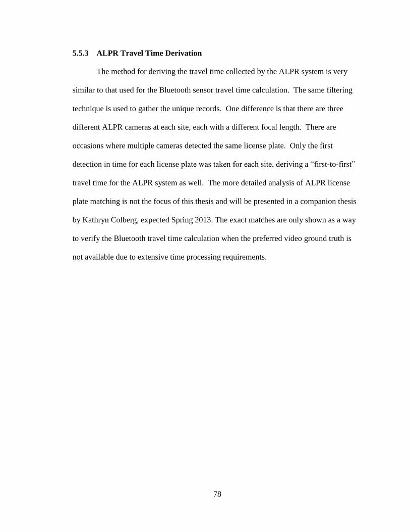
78
5.5.3 ALPR Travel Time Derivation
The method for deriving the travel time collected by the ALPR system is very
similar to that used for the Bluetooth sensor travel time calculation. The same filtering
technique is used to gather the unique records. One difference is that there are three
different ALPR cameras at each site, each with a different focal length. There are
occasions where multiple cameras detected the same license plate. Only the first
detection in time for each license plate was taken for each site, deriving a “first-to-first”
travel time for the ALPR system as well. The more detailed analysis of ALPR license
plate matching is not the focus of this thesis and will be presented in a companion thesis
by Kathryn Colberg, expected Spring 2013. The exact matches are only shown as a way
to verify the Bluetooth travel time calculation when the preferred video ground truth is
not available due to extensive time processing requirements.

79
Chapter 6: Results
6.1 Bluetooth Device and Sensor Characteristics Results
6.1.1 Single Sensor Capacity
The sensor capacity test series results show the device characteristics including
device detection pattern and the sensor ability to detect and increasing number of Class 1
and Class 2 Bluetooth-enabled devices. For the sensor capacity test series the script had
not yet been developed that records the cycle_start and cycle_end time stamps which
allow the research team to accurately count how many detections are taking place in each
cycle and in what pattern. Therefore, for the sensor capacity test series, the number of
cycle detections was calculated as an average based on the known cycle length of 11.24
seconds.
6.1.1.1 Class 2 Devices
First, Figure 27 below shows the number of device detections for each ten-minute
period as additional Class 2 devices were turned on in the single sensor’s field of view.
The blue dashed lane represents the mark of 53 cycles in each ten minute detection frame.
There is no noticeable decrease in the capacity of the sensor to detect the additional
devices, and the individual devices don’t show a trend toward decreasing detections with
up to 25 Class 2 devices, indicating that the sensor capacity has not yet been saturated by
the presence of 25 Class 2 Bluetooth devices. Next, Figure 28 and Figure 29 show the
headway frequency trend for device increments of five devices through 25 devices in 0.5
second bins.
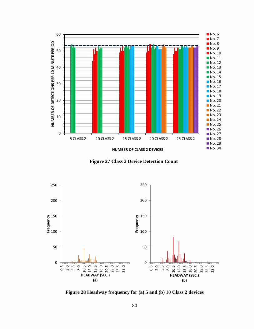
80
Figure 27 Class 2 Device Detection Count
Figure 28 Headway frequency for (a) 5 and (b) 10 Class 2 devices
0
10
20
30
40
50
60
5 CLASS 2 10 CLASS 2 15 CLASS 2 20 CLASS 2 25 CLASS 2
NU
MB
ER O
F D
ETEC
TIO
NS
PER
10
MIN
UTE
PER
IOD
NUMBER OF CLASS 2 DEVICES
No. 6No. 7No. 8No. 9No. 10No. 11No. 12No. 13No. 14No. 15No. 16No. 17No. 18No. 19No. 20No. 21No. 22No. 23No. 24No. 25No. 26No. 27No. 28No. 29No. 30
0
50
100
150
200
250
0.5
3.0
5.5
8.0
10
.5
13
.0
15
.5
18
.0
20
.5
23
.0
25
.5
28
.0
Fre
qu
en
cy
HEADWAY (SEC.) (a)
0
50
100
150
200
250
0.5
3.0
5.5
8.0
10
.5
13
.0
15
.5
18
.0
20
.5
23
.0
25
.5
28
.0
Fre
qu
en
cy
HEADWAY (SEC.) (b)

81
Figure 29 Headway frequency for (a) 15, (b) 20, and (c) 25 Class 2 devices
There is a common headway frequency peak trend for each set of the additional
five Class 2 Bluetooth devices approximately every 2.5 seconds. Thus devices were
0
50
100
150
200
250
0.5
3.0
5.5
8.0
10
.5
13
.0
15
.5
18
.0
20
.5
23
.0
25
.5
28
.0
Fre
qu
en
cy
HEADWAY (SEC.) (a)
0
50
100
150
200
250
0.5
3.0
5.5
8.0
10
.5
13
.0
15
.5
18
.0
20
.5
23
.0
25
.5
28
.0
Fre
qu
en
cy
HEADWAY (SEC.) (b)
0
50
100
150
200
250
0.5
3.0
5.5
8.0
10
.5
13
.0
15
.5
18
.0
20
.5
23
.0
25
.5
28
.0
Fre
qu
en
cy
HEADWAY (SEC.) (c)

82
redetected with eight second, 10.5 second, 13 second, and 15.5 second intervals. The 2.5
second trend is likely related to the inquiry subcycle duration of 1.28 seconds, with two
subcycles occurring every 2.56 seconds. The Figures show that the peak detection
interval is 10.5 seconds (approximately the length of one cycle) followed closely by 13
seconds. This indicates that Class 2 devices have a likelihood of being detected
approximately once per inquiry cycle.
6.1.1.2 Class 1 Devices
Figure 30 shows the detection count for each Class 1 device for the entire
deployment series of five through 25 devices. The shading is by device type, not by
every five device grouping as in the presentation above. Figure 30 shows that the sensor
capacity is not saturated by the presence of up to 25 Class 1 devices because the detection
count does not decrease with the introduction of an increasing number of Class 1 devices.
Rather, the detection count for 25 Class 1 devices is greater than for the preceding
grouping of 20 Class 1 devices.
Two of the Class 1 IOGear Bluetooth adaptors (R1 and R2) consistently exhibit
the detection count trend of a Class 2 device. Further investigation is required to
understand why Bluetooth adaptors R1 and R1 exhibit this trend. The remaining Class 1
devices have a detection count three to four times that of Class 2 devices, which is most
likely indicative of the transmission speeds for Class 1 devices being three times that of
Class 2 devices (3 Mbps vs. 1 Mbps).
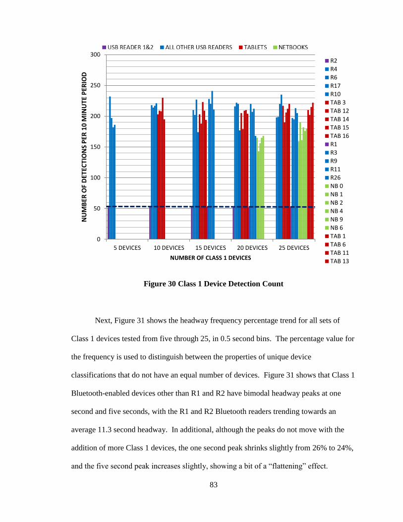
83
Figure 30 Class 1 Device Detection Count
Next, Figure 31 shows the headway frequency percentage trend for all sets of
Class 1 devices tested from five through 25, in 0.5 second bins. The percentage value for
the frequency is used to distinguish between the properties of unique device
classifications that do not have an equal number of devices. Figure 31 shows that Class 1
Bluetooth-enabled devices other than R1 and R2 have bimodal headway peaks at one
second and five seconds, with the R1 and R2 Bluetooth readers trending towards an
average 11.3 second headway. In additional, although the peaks do not move with the
addition of more Class 1 devices, the one second peak shrinks slightly from 26% to 24%,
and the five second peak increases slightly, showing a bit of a “flattening” effect.
0
50
100
150
200
250
300
5 DEVICES 10 DEVICES 15 DEVICES 20 DEVICES 25 DEVICES
NU
MB
ER O
F D
ETEC
TIO
NS
PER
10
MIN
UTE
PER
IOD
NUMBER OF CLASS 1 DEVICES
R2
R4
R6
R17
R10
TAB 3
TAB 12
TAB 14
TAB 15
TAB 16
R1
R3
R9
R11
R26
NB 0
NB 1
NB 2
NB 4
NB 9
NB 6
TAB 1
TAB 6
TAB 11
TAB 13
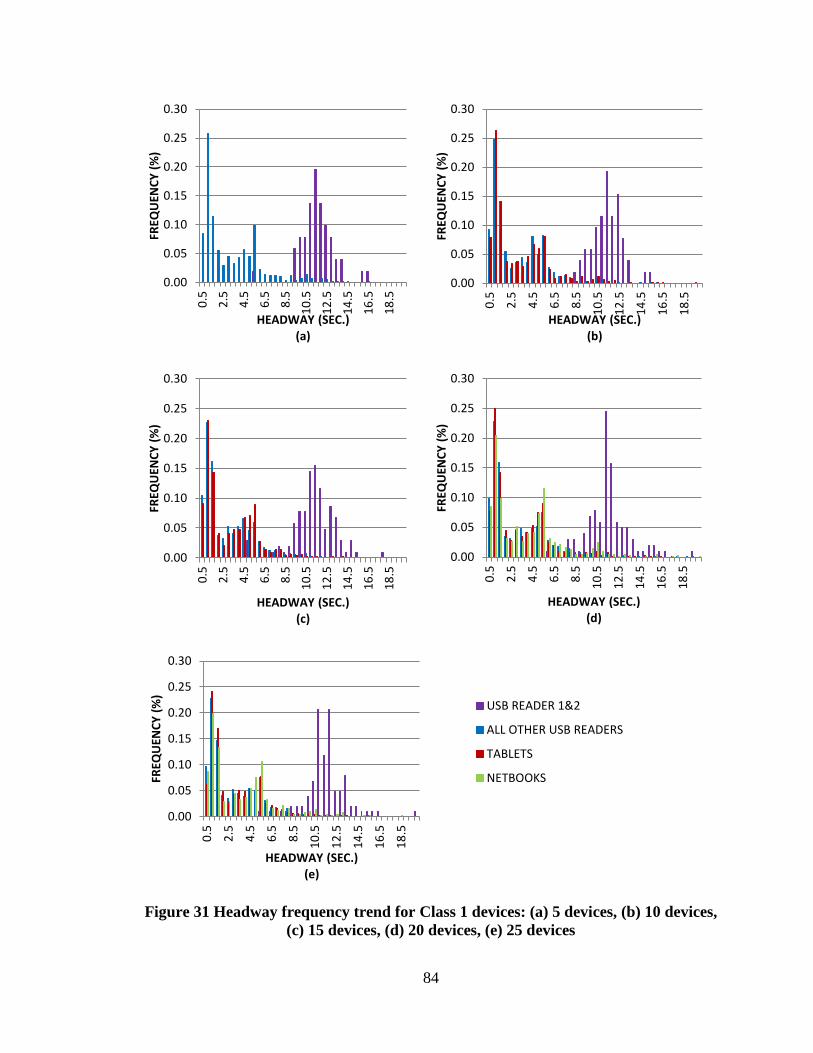
84
Figure 31 Headway frequency trend for Class 1 devices: (a) 5 devices, (b) 10 devices,
(c) 15 devices, (d) 20 devices, (e) 25 devices
0.00
0.05
0.10
0.15
0.20
0.25
0.30
0.5
2.5
4.5
6.5
8.5
10
.5
12
.5
14
.5
16
.5
18
.5
FREQ
UEN
CY
(%
)
HEADWAY (SEC.) (a)
0.00
0.05
0.10
0.15
0.20
0.25
0.30
0.5
2.5
4.5
6.5
8.5
10
.5
12
.5
14
.5
16
.5
18
.5
FREQ
UEN
CY
(%
)
HEADWAY (SEC.) (b)
0.00
0.05
0.10
0.15
0.20
0.25
0.30
0.5
2.5
4.5
6.5
8.5
10
.5
12
.5
14
.5
16
.5
18
.5
FREQ
UEN
CY
(%
)
HEADWAY (SEC.) (c)
0.00
0.05
0.10
0.15
0.20
0.25
0.30
0.5
2.5
4.5
6.5
8.5
10
.5
12
.5
14
.5
16
.5
18
.5
FREQ
UEN
CY
(%
)
HEADWAY (SEC.) (d)
0.00
0.05
0.10
0.15
0.20
0.25
0.30
0.5
2.5
4.5
6.5
8.5
10
.5
12
.5
14
.5
16
.5
18
.5
FREQ
UEN
CY
(%
)
HEADWAY (SEC.) (e)
USB READER 1&2
ALL OTHER USB READERS
TABLETS
NETBOOKS
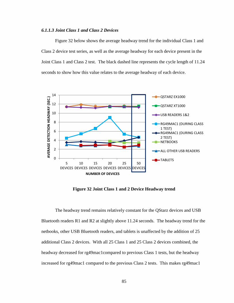
85
6.1.1.3 Joint Class 1 and Class 2 Devices
Figure 32 below shows the average headway trend for the individual Class 1 and
Class 2 device test series, as well as the average headway for each device present in the
Joint Class 1 and Class 2 test. The black dashed line represents the cycle length of 11.24
seconds to show how this value relates to the average headway of each device.
Figure 32 Joint Class 1 and 2 Device Headway trend
The headway trend remains relatively constant for the QStarz devices and USB
Bluetooth readers R1 and R2 at slightly above 11.24 seconds. The headway trend for the
netbooks, other USB Bluetooth readers, and tablets is unaffected by the addition of 25
additional Class 2 devices. With all 25 Class 1 and 25 Class 2 devices combined, the
headway decreased for rg49mac1compared to previous Class 1 tests, but the headway
increased for rg49mac1 compared to the previous Class 2 tests. This makes rg49mac1
0
2
4
6
8
10
12
14
5DEVICES
10DEVICES
15DEVICES
20DEVICES
25DEVICES
50DEVICES
AV
ERA
GE
DET
ECTI
ON
HEA
DW
AY
(SE
C.)
NUMBER OF DEVICES
QSTARZ EX1000
QSTARZ XT1000
USB READERS 1&2
RG49MAC1 (DURING CLASS1 TEST)RG49MAC1 (DURING CLASS2 TEST)NETBOOKS
ALL OTHER USB READERS
TABLETS
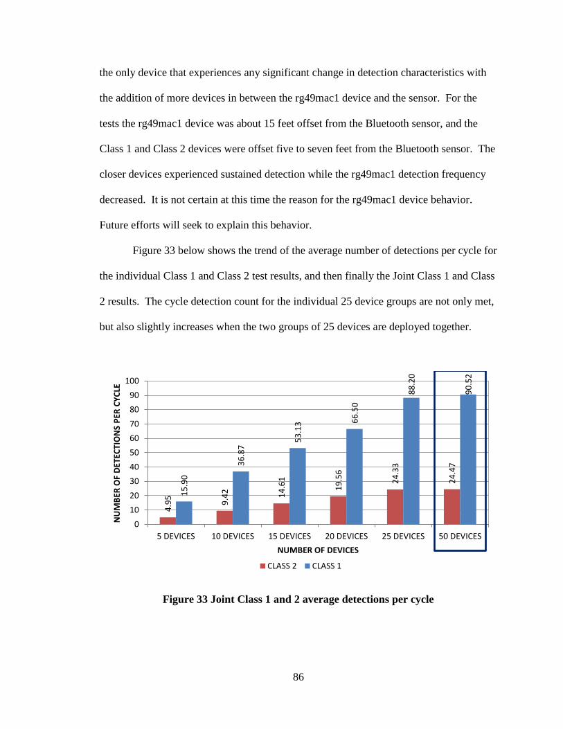
86
the only device that experiences any significant change in detection characteristics with
the addition of more devices in between the rg49mac1 device and the sensor. For the
tests the rg49mac1 device was about 15 feet offset from the Bluetooth sensor, and the
Class 1 and Class 2 devices were offset five to seven feet from the Bluetooth sensor. The
closer devices experienced sustained detection while the rg49mac1 detection frequency
decreased. It is not certain at this time the reason for the rg49mac1 device behavior.
Future efforts will seek to explain this behavior.
Figure 33 below shows the trend of the average number of detections per cycle for
the individual Class 1 and Class 2 test results, and then finally the Joint Class 1 and Class
2 results. The cycle detection count for the individual 25 device groups are not only met,
but also slightly increases when the two groups of 25 devices are deployed together.
Figure 33 Joint Class 1 and 2 average detections per cycle
4.9
5
9.4
2
14
.61
19
.56
24
.33
24
.47
15
.90
36
.87
53
.13
66
.50
88
.20
90
.52
0
10
20
30
40
50
60
70
80
90
100
5 DEVICES 10 DEVICES 15 DEVICES 20 DEVICES 25 DEVICES 50 DEVICES
NU
MB
ER O
F D
ETEC
TIO
NS
PER
CY
CLE
NUMBER OF DEVICES
CLASS 2 CLASS 1

87
These results show that 50 devices is not yet the point of saturation for the Class 1
custom Bluetooth sensor. Following, Figure 34 shows the average detections per cycle
separated into device type. The Class 1 devices consistently have greater detections per
cycle than Class 2 devices by three to four times (again indicative of the different
transmission speeds). Furthermore, there is a relative consistency of cycle detection
count as more Bluetooth-enabled devices are placed in the sensor’s field of view. This
demonstrates further than 50 devices do not appear to reach single sensor saturation.
Figure 34 Joint Class 1 and 2 average detections per cycle by device type
6.1.2 Multiple Sensor Effect
Figure 35 and Figure 36 below show the detection count for each Class 2 device
in each ten minute detection period incrementing from five to 20 Class 2 devices for
Sensor 5 and Sensor 8, respectively.
0.00
0.50
1.00
1.50
2.00
2.50
3.00
3.50
4.00
4.50
5DEVICES
10DEVICES
15DEVICES
20DEVICES
25DEVICES
50DEVICES
AV
ERA
GE
DET
ECTI
ON
S P
ER C
YC
LE P
ER D
EVIC
E
NUMBER OF DEVICES
QSTARZ EX1000
QSTARZ XT1000
USB READERS 1&2
RG49MAC1 (DURINGCLASS 1 TEST)NETBOOKS
ALL OTHER USB READERS
TABLETS
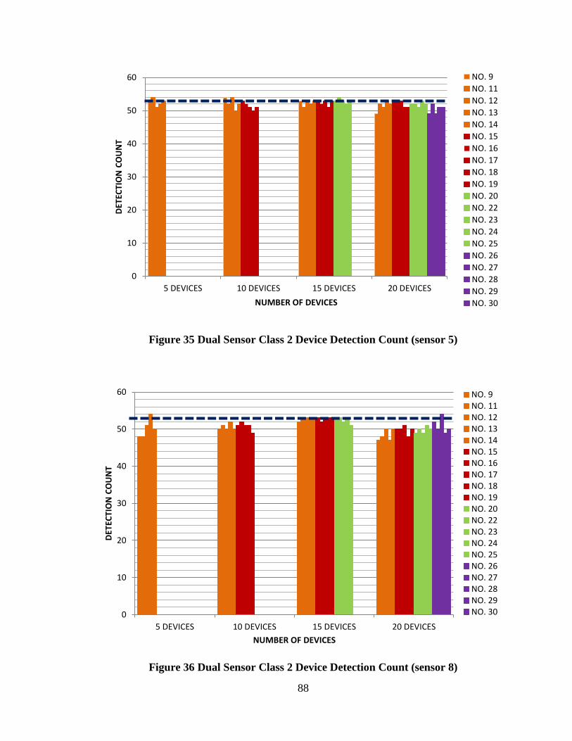
88
Figure 35 Dual Sensor Class 2 Device Detection Count (sensor 5)
Figure 36 Dual Sensor Class 2 Device Detection Count (sensor 8)
0
10
20
30
40
50
60
5 DEVICES 10 DEVICES 15 DEVICES 20 DEVICES
DET
ECTI
ON
CO
UN
T
NUMBER OF DEVICES
NO. 9
NO. 11
NO. 12
NO. 13
NO. 14
NO. 15
NO. 16
NO. 17
NO. 18
NO. 19
NO. 20
NO. 22
NO. 23
NO. 24
NO. 25
NO. 26
NO. 27
NO. 28
NO. 29
NO. 30
0
10
20
30
40
50
60
5 DEVICES 10 DEVICES 15 DEVICES 20 DEVICES
DET
ECTI
ON
CO
UN
T
NUMBER OF DEVICES
NO. 9NO. 11NO. 12NO. 13NO. 14NO. 15NO. 16NO. 17NO. 18NO. 19NO. 20NO. 22NO. 23NO. 24NO. 25NO. 26NO. 27NO. 28NO. 29NO. 30
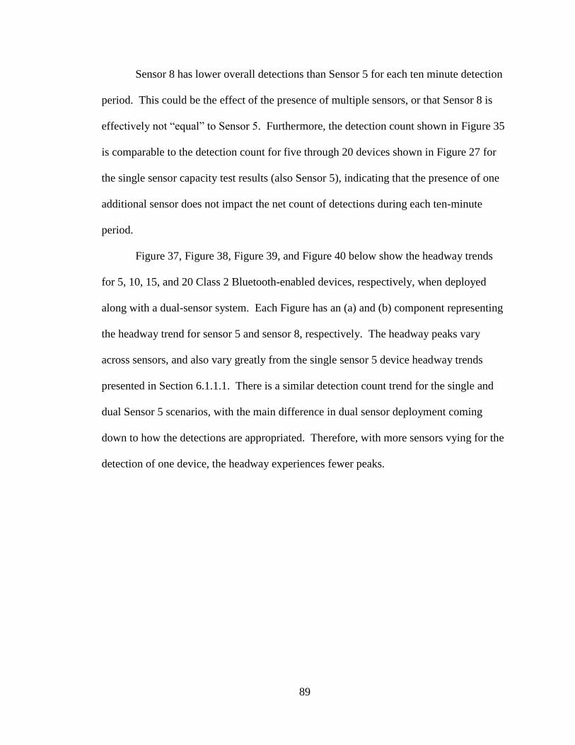
89
Sensor 8 has lower overall detections than Sensor 5 for each ten minute detection
period. This could be the effect of the presence of multiple sensors, or that Sensor 8 is
effectively not “equal” to Sensor 5. Furthermore, the detection count shown in Figure 35
is comparable to the detection count for five through 20 devices shown in Figure 27 for
the single sensor capacity test results (also Sensor 5), indicating that the presence of one
additional sensor does not impact the net count of detections during each ten-minute
period.
Figure 37, Figure 38, Figure 39, and Figure 40 below show the headway trends
for 5, 10, 15, and 20 Class 2 Bluetooth-enabled devices, respectively, when deployed
along with a dual-sensor system. Each Figure has an (a) and (b) component representing
the headway trend for sensor 5 and sensor 8, respectively. The headway peaks vary
across sensors, and also vary greatly from the single sensor 5 device headway trends
presented in Section 6.1.1.1. There is a similar detection count trend for the single and
dual Sensor 5 scenarios, with the main difference in dual sensor deployment coming
down to how the detections are appropriated. Therefore, with more sensors vying for the
detection of one device, the headway experiences fewer peaks.
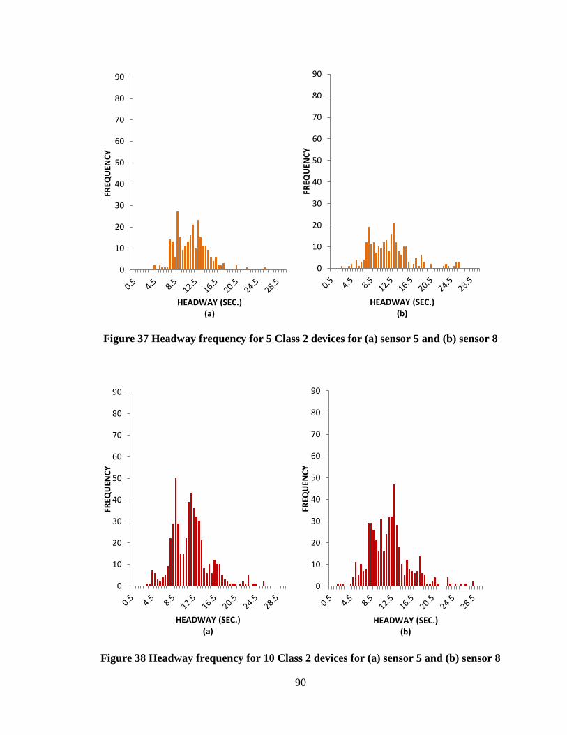
90
Figure 37 Headway frequency for 5 Class 2 devices for (a) sensor 5 and (b) sensor 8
Figure 38 Headway frequency for 10 Class 2 devices for (a) sensor 5 and (b) sensor 8
0
10
20
30
40
50
60
70
80
90
FREQ
UEN
CY
HEADWAY (SEC.) (a)
0
10
20
30
40
50
60
70
80
90
FREQ
UEN
CY
HEADWAY (SEC.)
(b)
0
10
20
30
40
50
60
70
80
90
FREQ
UEN
CY
HEADWAY (SEC.) (a)
0
10
20
30
40
50
60
70
80
90
FREQ
UEN
CY
HEADWAY (SEC.) (b)
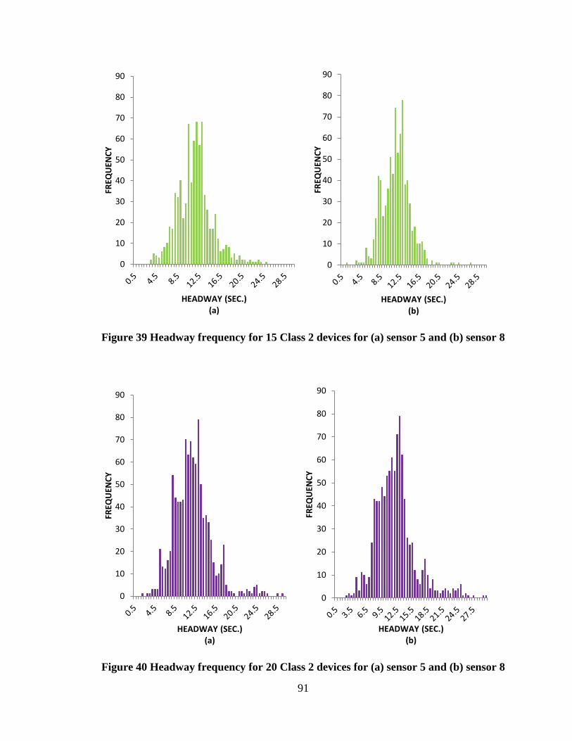
91
Figure 39 Headway frequency for 15 Class 2 devices for (a) sensor 5 and (b) sensor 8
Figure 40 Headway frequency for 20 Class 2 devices for (a) sensor 5 and (b) sensor 8
0
10
20
30
40
50
60
70
80
90
FREQ
UEN
CY
HEADWAY (SEC.) (a)
0
10
20
30
40
50
60
70
80
90
FREQ
UEN
CY
HEADWAY (SEC.) (b)
0
10
20
30
40
50
60
70
80
90
FREQ
UEN
CY
HEADWAY (SEC.) (a)
0
10
20
30
40
50
60
70
80
90
FREQ
UEN
CY
HEADWAY (SEC.) (b)
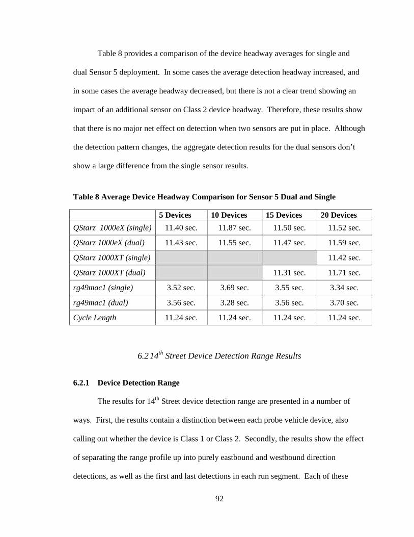
92
Table 8 provides a comparison of the device headway averages for single and
dual Sensor 5 deployment. In some cases the average detection headway increased, and
in some cases the average headway decreased, but there is not a clear trend showing an
impact of an additional sensor on Class 2 device headway. Therefore, these results show
that there is no major net effect on detection when two sensors are put in place. Although
the detection pattern changes, the aggregate detection results for the dual sensors don’t
show a large difference from the single sensor results.
Table 8 Average Device Headway Comparison for Sensor 5 Dual and Single
5 Devices 10 Devices 15 Devices 20 Devices
QStarz 1000eX (single) 11.40 sec. 11.87 sec. 11.50 sec. 11.52 sec.
QStarz 1000eX (dual) 11.43 sec. 11.55 sec. 11.47 sec. 11.59 sec.
QStarz 1000XT (single)
11.42 sec.
QStarz 1000XT (dual) 11.31 sec. 11.71 sec.
rg49mac1 (single) 3.52 sec. 3.69 sec. 3.55 sec. 3.34 sec.
rg49mac1 (dual) 3.56 sec. 3.28 sec. 3.56 sec. 3.70 sec.
Cycle Length 11.24 sec. 11.24 sec. 11.24 sec. 11.24 sec.
6.2 14th
Street Device Detection Range Results
6.2.1 Device Detection Range
The results for 14th
Street device detection range are presented in a number of
ways. First, the results contain a distinction between each probe vehicle device, also
calling out whether the device is Class 1 or Class 2. Secondly, the results show the effect
of separating the range profile up into purely eastbound and westbound direction
detections, as well as the first and last detections in each run segment. Each of these

93
distinctions is made for the midblock and intersection sensor locations in the following
sections. The reason for separating the results into these different categories is to see if a
pattern arises in any category, and to assess which detection characteristic to use when
calculating travel time along a corridor.
6.2.1.1 Detection Range Influencing Factors
There are two main factors that play a role in the detection range results presented
in the following results. The first is how the physical boundary of the run corridor is
defined, and the second is how the beginning and end of a run coincides with the
beginning or end of an inquiry cycle.
6.2.1.1.1 Physical Run Boundary
After the initial analysis, the research team chose to redefine the physical limits of
the run to end 100 feet before the two turnaround locations on the 14th
Street corridor.
The reasoning behind this decision is that the probe vehicles were stationary at the
turnaround locations for anywhere from five seconds to over 60 seconds. During this
time the probe vehicles were not actively on the corridor, and were also present at the
same location for portions of the eastbound and westbound legs of each run. In addition,
the probe vehicle devices were not in motion on the corridor, which contradicts the goal
of this analysis to assess the best method of calculating real-time travel time.
Furthermore, stationary Bluetooth-enabled devices do have a higher propensity for
detection than devices in motion when within a sensor’s field of view.
By narrowing the window of the corridor by 100 feet before each turn around
location, the revised window of the detection corridor is 811 feet west of the midblock

94
location, and 1220 feet east of the intersection location. However, to be consistent with
defining the extents of the corridor around the midblock and intersection sensor locations,
the research team opted to narrow the corridor span to 800 feet on the eastbound end of
the intersection sensor and 800 feet on the westbound end of the midblock sensor.
Although these adjustments were made for the majority of the analysis, the initial results
show the raw data including all detections occurring near-to and within TA1 and TA2.
6.2.1.1.2 Run Time and Inquiry Cycle
The results show a correlation between continued device detection and the sensor
inquiry cycle. A string of detections including anywhere from two to eight detections at
the midblock and up to 18 detection at the intersection occur all within the same sensor
inquiry cycle. Once the sensor detects a device, a communication stream has been
established between the two where ongoing detection occurs. Surprisingly, this ongoing
detection continues even as the device leaves the 300 foot detection window for the
Bluetooth sensor to as far out as 1000 feet, particularly for Class 1 devices, as the results
of the 14th
Street test show below.
6.2.1.2 Friday, August 24, 2012
6.2.1.2.1 All Detections
On Friday, August 24th
, the probe vehicles completed 27 runs (each with an
eastbound and westbound leg) along the 14th
Street corridor. Figure 41below shows all
of the detections, eastbound and westbound, including multiple detections, for the
midblock Bluetooth sensor. The black dashed line shows the location of the sensor of
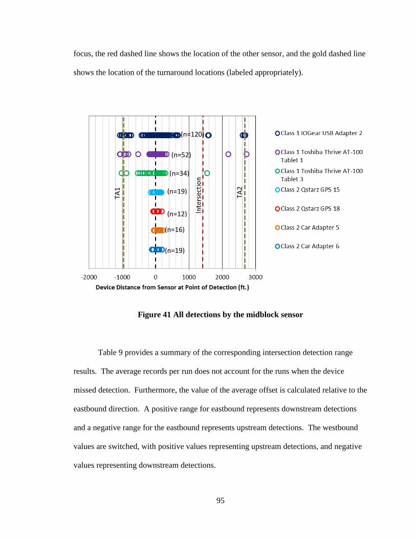
95
focus, the red dashed line shows the location of the other sensor, and the gold dashed line
shows the location of the turnaround locations (labeled appropriately).
Figure 41 All detections by the midblock sensor
Table 9 provides a summary of the corresponding intersection detection range
results. The average records per run does not account for the runs when the device
missed detection. Furthermore, the value of the average offset is calculated relative to the
eastbound direction. A positive range for eastbound represents downstream detections
and a negative range for the eastbound represents upstream detections. The westbound
values are switched, with positive values representing upstream detections, and negative
values representing downstream detections.
TA2
TA1
(n=120)
(n=52)
(n=34)
(n=19)
(n=12)
(n=16)
(n=19)
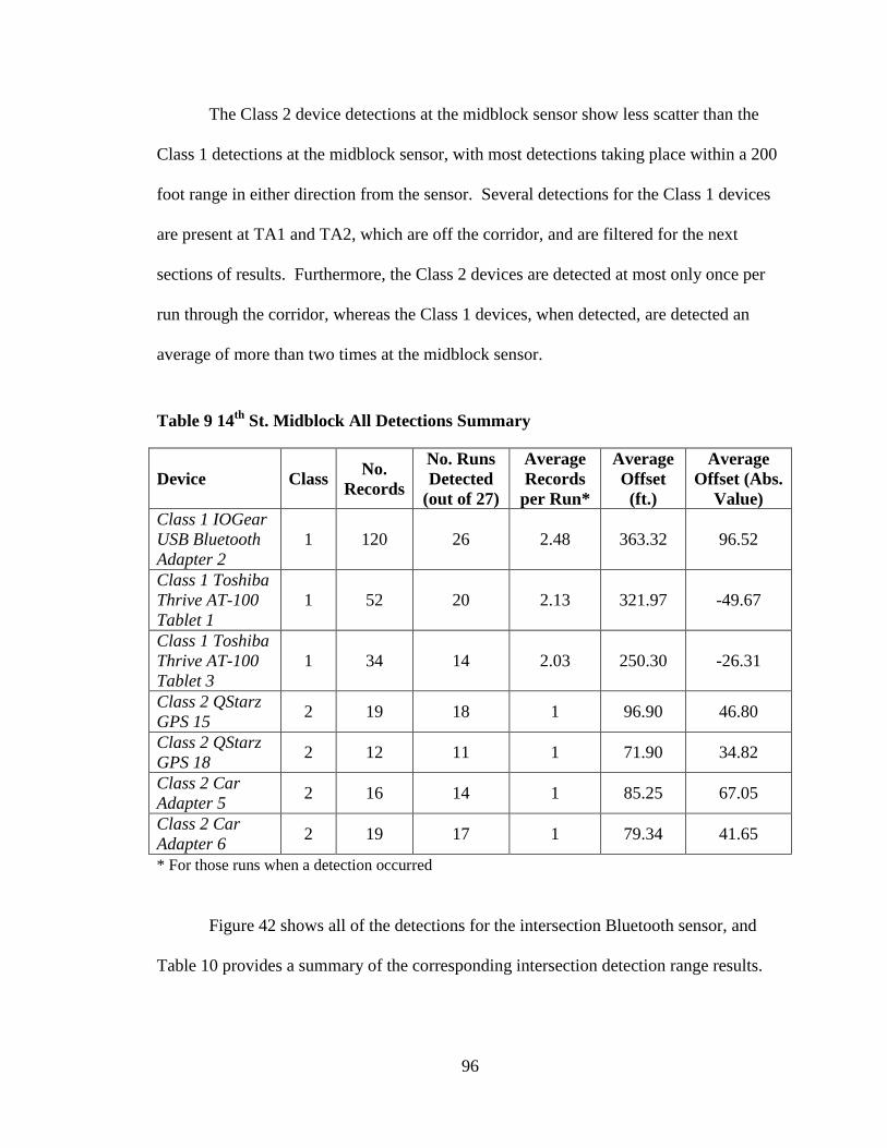
96
The Class 2 device detections at the midblock sensor show less scatter than the
Class 1 detections at the midblock sensor, with most detections taking place within a 200
foot range in either direction from the sensor. Several detections for the Class 1 devices
are present at TA1 and TA2, which are off the corridor, and are filtered for the next
sections of results. Furthermore, the Class 2 devices are detected at most only once per
run through the corridor, whereas the Class 1 devices, when detected, are detected an
average of more than two times at the midblock sensor.
Table 9 14th
St. Midblock All Detections Summary
Device Class No.
Records
No. Runs
Detected
(out of 27)
Average
Records
per Run*
Average
Offset
(ft.)
Average
Offset (Abs.
Value)
Class 1 IOGear
USB Bluetooth
Adapter 2
1 120 26 2.48 363.32 96.52
Class 1 Toshiba
Thrive AT-100
Tablet 1
1 52 20 2.13 321.97 -49.67
Class 1 Toshiba
Thrive AT-100
Tablet 3
1 34 14 2.03 250.30 -26.31
Class 2 QStarz
GPS 15 2 19 18 1 96.90 46.80
Class 2 QStarz
GPS 18 2 12 11 1 71.90 34.82
Class 2 Car
Adapter 5 2 16 14 1 85.25 67.05
Class 2 Car
Adapter 6 2 19 17 1 79.34 41.65
* For those runs when a detection occurred
Figure 42 shows all of the detections for the intersection Bluetooth sensor, and
Table 10 provides a summary of the corresponding intersection detection range results.
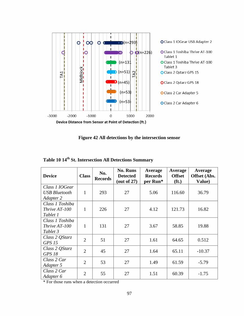
97
Figure 42 All detections by the intersection sensor
Table 10 14th
St. Intersection All Detections Summary
Device Class No.
Records
No. Runs
Detected
(out of 27)
Average
Records
per Run*
Average
Offset
(ft.)
Average
Offset (Abs.
Value)
Class 1 IOGear
USB Bluetooth
Adapter 2
1 293 27 5.06 116.60 36.79
Class 1 Toshiba
Thrive AT-100
Tablet 1
1 226 27 4.12 121.73 16.82
Class 1 Toshiba
Thrive AT-100
Tablet 3
1 131 27 3.67 58.85 19.88
Class 2 QStarz
GPS 15 2 51 27 1.61 64.65 0.512
Class 2 QStarz
GPS 18 2 45 27 1.64 65.11 -10.37
Class 2 Car
Adapter 5 2 53 27 1.49 61.59 -5.79
Class 2 Car
Adapter 6 2 55 27 1.51 60.39 -1.75
* For those runs when a detection occurred
TA2
TA1
(n=293)
(n=226)
(n=131
) (n=51)
(n=45)
(n=53)
(n=53)

98
The intersection detections for the Class 2 devices and Toshiba Tablet 3 show
very little scatter, and are all concentrated within a 200 foot detection range around the
intersection sensor. Similar to the midblock detections, the Class 1 devices show some
variability for intersection detections, and have detections at TA1 and TA2, which are
again filtered for the next sections of results. The intersection detections show on
average more detections per run than for the midblock detections. This is likely due to
the stop-and-go nature of the intersection traffic operations. The slowing/stopping of the
vehicles maintained the device in the sensor’s field of view for a longer period of time,
most often more than one cycle, allowing for an average increase in the number of
detections per run. Conversely, the vehicles passing the midblock sensor were always in
free flow in the eastbound and westbound directions.
6.2.1.2.2 Eastbound All Detections
Figure 43 below shows all eastbound detections for the midblock sensor, and
Table 11 provides a summary of corresponding midblock sensor detection range results.
Following, Figure 44 shows all eastbound detections for the intersection sensor, and
Table 12 provides a summary of the corresponding intersection detection range results.
These results follow the corridor span modification, showing detections only 800 feet
west of the midblock sensor. After a close inspection of the results, those detections that
are taking place outside of the expected 300 foot detection range are typically part of a
Class 1 detection “string”, which consists of repeat detections within the same 11.24
second sensor inquiry cycle.

99
Figure 43 All Eastbound detections by the midblock sensor
Table 11 14th
St. Midblock Eastbound All Detections Summary
Device Class No.
Records
No. Runs
Detected
(out of 27)
Average
Records
per Run*
Average
Offset
(ft.)
Average
Offset (Abs.
Value)
Class 1 IOGear
USB Bluetooth
Adapter 2
1 50 20 2.54 133.67 218.61
Class 1 Toshiba
Thrive AT-100
Tablet 1
1 22 13 2.20 128.82 235.82
Class 1 Toshiba
Thrive AT-100
Tablet 3
1 19 12 2.03 101.99 101.99
Class 2 QStarz
GPS 15 2 12 12 1 96.73 104.26
Class 2 QStarz
GPS 18 2 7 7 1 82.99 82.99
Class 2 Car
Adapter 5 2 12 12 1 90.81 95.78
Class 2 Car
Adapter 6 2 15 15 1 76.63 72.63
* For those runs when a detection occurred
(n=50)
(n=22)
(n=19)
(n=12)
(n=7)
(n=12)
(n=15)
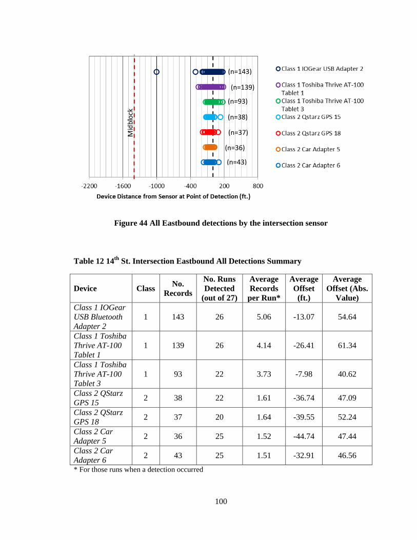
100
Figure 44 All Eastbound detections by the intersection sensor
Table 12 14th
St. Intersection Eastbound All Detections Summary
Device Class No.
Records
No. Runs
Detected
(out of 27)
Average
Records
per Run*
Average
Offset
(ft.)
Average
Offset (Abs.
Value)
Class 1 IOGear
USB Bluetooth
Adapter 2
1 143 26 5.06 -13.07 54.64
Class 1 Toshiba
Thrive AT-100
Tablet 1
1 139 26 4.14 -26.41 61.34
Class 1 Toshiba
Thrive AT-100
Tablet 3
1 93 22 3.73 -7.98 40.62
Class 2 QStarz
GPS 15 2 38 22 1.61 -36.74 47.09
Class 2 QStarz
GPS 18 2 37 20 1.64 -39.55 52.24
Class 2 Car
Adapter 5 2 36 25 1.52 -44.74 47.44
Class 2 Car
Adapter 6 2 43 25 1.51 -32.91 46.56
* For those runs when a detection occurred
(n=143)
(n=139)
(n=93)
(n=38)
(n=37)
(n=36)
(n=43)
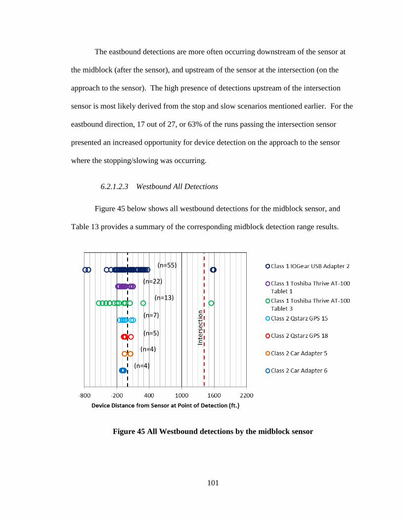
101
The eastbound detections are more often occurring downstream of the sensor at
the midblock (after the sensor), and upstream of the sensor at the intersection (on the
approach to the sensor). The high presence of detections upstream of the intersection
sensor is most likely derived from the stop and slow scenarios mentioned earlier. For the
eastbound direction, 17 out of 27, or 63% of the runs passing the intersection sensor
presented an increased opportunity for device detection on the approach to the sensor
where the stopping/slowing was occurring.
6.2.1.2.3 Westbound All Detections
Figure 45 below shows all westbound detections for the midblock sensor, and
Table 13 provides a summary of the corresponding midblock detection range results.
Figure 45 All Westbound detections by the midblock sensor
(n=55)
(n=22)
(n=13)
(n=7)
(n=5)
(n=4)
(n=4)

102
Table 13 14th
St. Midblock Westbound All Detections Summary
Device Class No.
Records
No. Runs
Detected
(out of 27)
Average
Records
per Run*
Average
Offset
(ft.)
Average
Offset (Abs.
Value)
Class 1 IOGear
USB Bluetooth
Adapter 2
1 55 21 2.48 69.63 221.32
Class 1 Toshiba
Thrive AT-100
Tablet 1
1 22 13 2.16 -68.76 100.21
Class 1 Toshiba
Thrive AT-100
Tablet 3
1 13 6 2.13 -71.29 359.00
Class 2 QStarz
GPS 15 2 7 7 1 -38.82 84.29
Class 2 QStarz
GPS 18 2 5 5 1 -32.62 56.36
Class 2 Car
Adapter 5 2 4 4 1 -4.23 53.67
Class 2 Car
Adapter 6 2 4 4 1 -89.50 89.50
* For those runs when a detection occurred
As shown in Figure 45 and Table 13, the westbound midblock detections still
experience a large amount of scatter, particularly for the Class 1 devices. The spread is
both upstream and downstream of the midblock sensor, but Class 2 devices show a
greater likelihood for detection downstream of the midblock sensor. However, the
number of records of detection is significantly less for the westbound midblock than the
eastbound midblock. This is most likely because the westbound devices are farther from
the sensor than the eastbound devices, so their likelihood and frequency of detection
decreases.
Next, Figure 46 shows all westbound detections for the intersection sensor, and
Table 14 provides a summary of the corresponding intersection detection range results.
The westbound intersection detections experience significantly more scatter than the
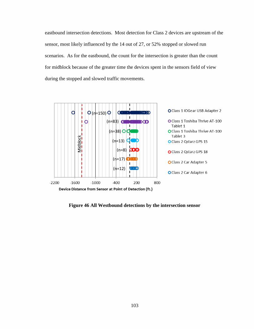
103
eastbound intersection detections. Most detection for Class 2 devices are upstream of the
sensor, most likely influenced by the 14 out of 27, or 52% stopped or slowed run
scenarios. As for the eastbound, the count for the intersection is greater than the count
for midblock because of the greater time the devices spent in the sensors field of view
during the stopped and slowed traffic movements.
Figure 46 All Westbound detections by the intersection sensor
(n=150)
(n=83)
(n=38)
(n=13)
(n=8)
(n=17)
(n=12)
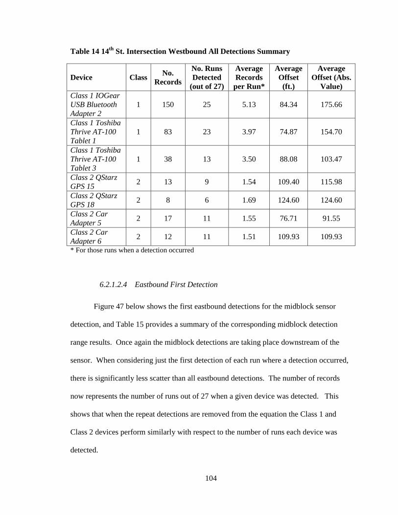
104
Table 14 14th
St. Intersection Westbound All Detections Summary
Device Class No.
Records
No. Runs
Detected
(out of 27)
Average
Records
per Run*
Average
Offset
(ft.)
Average
Offset (Abs.
Value)
Class 1 IOGear
USB Bluetooth
Adapter 2
1 150 25 5.13 84.34 175.66
Class 1 Toshiba
Thrive AT-100
Tablet 1
1 83 23 3.97 74.87 154.70
Class 1 Toshiba
Thrive AT-100
Tablet 3
1 38 13 3.50 88.08 103.47
Class 2 QStarz
GPS 15 2 13 9 1.54 109.40 115.98
Class 2 QStarz
GPS 18 2 8 6 1.69 124.60 124.60
Class 2 Car
Adapter 5 2 17 11 1.55 76.71 91.55
Class 2 Car
Adapter 6 2 12 11 1.51 109.93 109.93
* For those runs when a detection occurred
6.2.1.2.4 Eastbound First Detection
Figure 47 below shows the first eastbound detections for the midblock sensor
detection, and Table 15 provides a summary of the corresponding midblock detection
range results. Once again the midblock detections are taking place downstream of the
sensor. When considering just the first detection of each run where a detection occurred,
there is significantly less scatter than all eastbound detections. The number of records
now represents the number of runs out of 27 when a given device was detected. This
shows that when the repeat detections are removed from the equation the Class 1 and
Class 2 devices perform similarly with respect to the number of runs each device was
detected.

105
Figure 47 First Eastbound detection in each run by the midblock sensor
Table 15 14th
St. Midblock Eastbound First Detections Summary
Device Class
No. Runs
Detected (out
of 27)
Average
Offset (ft.)
Average Offset
(Abs. Value)
Class 1 IOGear USB
Bluetooth Adapter 2 1 18 -9.63 148.34
Class 1 Toshiba Thrive
AT-100 Tablet 1 1 12 -37.57 129.68
Class 1 Toshiba Thrive
AT-100 Tablet 3 1 11 72.33 72.33
Class 2 QStarz GPS 15 2 12 96.73 104.26
Class 2 QStarz GPS 18 2 7 82.99 82.99
Class 2 Car Adapter 5 2 12 90.81 95.78
Class 2 Car Adapter 6 2 15 76.63 72.63
Next, Figure 48 shows the first eastbound detections for the intersection sensor,
and Table 16 provides a summary of the corresponding detection range results. Once
(n=18)
(n=12)
(n=11)
(n=12)
(n=7)
(n=12)
(n=15)

106
again the intersection detections are taking place upstream of the sensor. All devices are
detected in a greater portion of the runs for the intersection than the midblock, with GPS
18 missing the most runs at seven. This higher run detection rate is most likely the result
of 63% of the runs featuring stopped or slowed traffic scenarios. There is also
significantly less scatter for the intersection detection when only the first detection in
each run per device is considered as opposed to all eastbound intersection detections.
Figure 48 First Eastbound detection in each run by the intersection sensor
(n=26)
(n=26)
(n=22)
(n=22)
(n=20)
(n=23)
(n=25)

107
Table 16 14th
St. Intersection Eastbound First Detections Summary
Device Class
No. Runs
Detected (out
of 27)
Average
Offset (ft.)
Average Offset
(Abs. Value)
Class 1 IOGear USB
Bluetooth Adapter 2 1 26 -100.66 118.99
Class 1 Toshiba Thrive
AT-100 Tablet 1 1 26 -87.25 100.60
Class 1 Toshiba Thrive
AT-100 Tablet 3 1 22 -55.32 59.05
Class 2 QStarz GPS 15 2 22 -43.13 59.38
Class 2 QStarz GPS 18 2 20 -73.14 75.10
Class 2 Car Adapter 5 2 23 -54.18 56.85
Class 2 Car Adapter 6 2 25 -61.43 66.35
6.2.1.2.5 Westbound First Detection
Figure 49 below shows the first westbound detections for the midblock sensor,
and Table 17 provides a summary of the corresponding detection range results. The
number of records for this case also represents the number of runs out of 27 that a given
device was detected. The westbound first detections are distributed around the sensor,
but they still show a propensity for detection downstream of the sensor when traveling
westbound, as the average offset shows. The number of runs detected for each device
shows a great discrepancy in the detection frequency of Class 1 versus Class 2 devices.
This is most likely because Class 1 devices are of a higher power class, and thus have a
greater ability to communicate across longer distances than Class 2 devices.
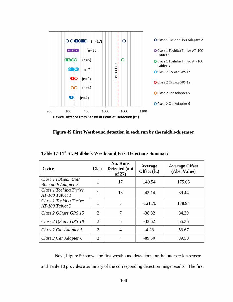
108
Figure 49 First Westbound detection in each run by the midblock sensor
Table 17 14th
St. Midblock Westbound First Detections Summary
Device Class
No. Runs
Detected (out
of 27)
Average
Offset (ft.)
Average Offset
(Abs. Value)
Class 1 IOGear USB
Bluetooth Adapter 2 1 17 140.54 175.66
Class 1 Toshiba Thrive
AT-100 Tablet 1 1 13 -43.14 89.44
Class 1 Toshiba Thrive
AT-100 Tablet 3 1 5 -121.70 138.94
Class 2 QStarz GPS 15 2 7 -38.82 84.29
Class 2 QStarz GPS 18 2 5 -32.62 56.36
Class 2 Car Adapter 5 2 4 -4.23 53.67
Class 2 Car Adapter 6 2 4 -89.50 89.50
Next, Figure 50 shows the first westbound detections for the intersection sensor,
and Table 18 provides a summary of the corresponding detection range results. The first
(n=17)
(n=13)
(n=5)
(n=7)
(n=5)
(n=4)
(n=4)
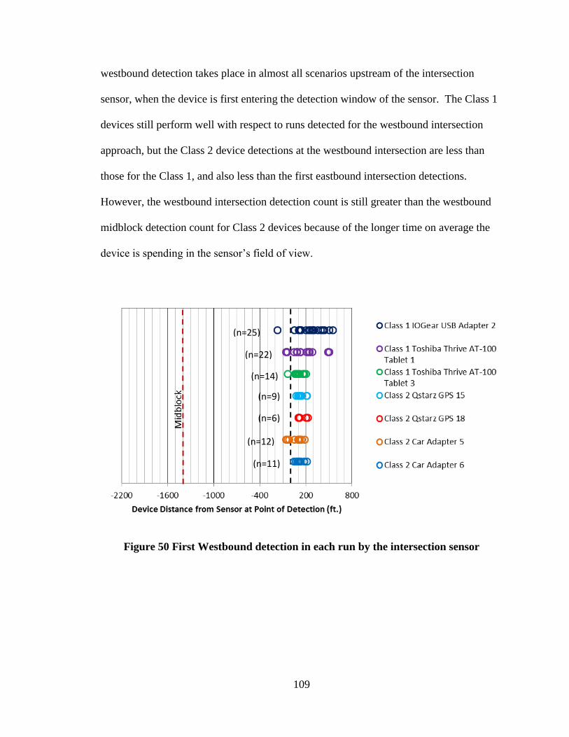
109
westbound detection takes place in almost all scenarios upstream of the intersection
sensor, when the device is first entering the detection window of the sensor. The Class 1
devices still perform well with respect to runs detected for the westbound intersection
approach, but the Class 2 device detections at the westbound intersection are less than
those for the Class 1, and also less than the first eastbound intersection detections.
However, the westbound intersection detection count is still greater than the westbound
midblock detection count for Class 2 devices because of the longer time on average the
device is spending in the sensor’s field of view.
Figure 50 First Westbound detection in each run by the intersection sensor
(n=25)
(n=22)
(n=14)
(n=9)
(n=6)
(n=12)
(n=11)
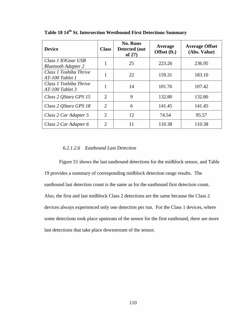
110
Table 18 14th
St. Intersection Westbound First Detections Summary
Device Class
No. Runs
Detected (out
of 27)
Average
Offset (ft.)
Average Offset
(Abs. Value)
Class 1 IOGear USB
Bluetooth Adapter 2 1 25 223.26 236.95
Class 1 Toshiba Thrive
AT-100 Tablet 1 1 22 159.31 183.10
Class 1 Toshiba Thrive
AT-100 Tablet 3 1 14 101.76 107.42
Class 2 QStarz GPS 15 2 9 132.80 132.80
Class 2 QStarz GPS 18 2 6 141.45 141.45
Class 2 Car Adapter 5 2 12 74.54 95.57
Class 2 Car Adapter 6 2 11 110.38 110.38
6.2.1.2.6 Eastbound Last Detection
Figure 51 shows the last eastbound detections for the midblock sensor, and Table
19 provides a summary of corresponding midblock detection range results. The
eastbound last detection count is the same as for the eastbound first detection count.
Also, the first and last midblock Class 2 detections are the same because the Class 2
devices always experienced only one detection per run. For the Class 1 devices, where
some detections took place upstream of the sensor for the first eastbound, there are more
last detections that take place downstream of the sensor.
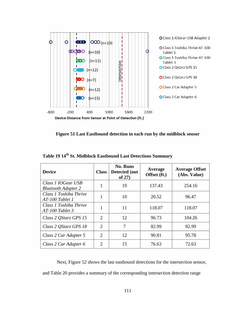
111
Figure 51 Last Eastbound detection in each run by the midblock sensor
Table 19 14th
St. Midblock Eastbound Last Detections Summary
Device Class
No. Runs
Detected (out
of 27)
Average
Offset (ft.)
Average Offset
(Abs. Value)
Class 1 IOGear USB
Bluetooth Adapter 2 1 19 137.43 254.16
Class 1 Toshiba Thrive
AT-100 Tablet 1 1 10 20.52 96.47
Class 1 Toshiba Thrive
AT-100 Tablet 3 1 11 118.07 118.07
Class 2 QStarz GPS 15 2 12 96.73 104.26
Class 2 QStarz GPS 18 2 7 82.99 82.99
Class 2 Car Adapter 5 2 12 90.81 95.78
Class 2 Car Adapter 6 2 15 76.63 72.63
Next, Figure 52 shows the last eastbound detections for the intersection sensor,
and Table 20 provides a summary of the corresponding intersection detection range
(n=19)
(n=10)
(n=11)
(n=12)
(n=7)
(n=12)
(n=15)

112
results. The last detection at the intersection sensor takes place more often downstream
of the intersection sensor for Class 1 devices; and upstream of the intersection sensor for
the Class 2 devices. There is also more scatter for the midblock detections than for the
corresponding intersection detections.
Figure 52 Last Eastbound detection in each run by the intersection sensor
(n=26)
(n=26)
(n=22)
(n=22)
(n=20)
(n=24)
(n=25)
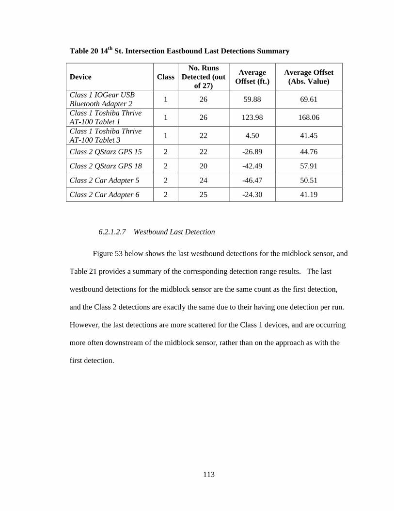
113
Table 20 14th
St. Intersection Eastbound Last Detections Summary
Device Class
No. Runs
Detected (out
of 27)
Average
Offset (ft.)
Average Offset
(Abs. Value)
Class 1 IOGear USB
Bluetooth Adapter 2 1 26 59.88 69.61
Class 1 Toshiba Thrive
AT-100 Tablet 1 1 26 123.98 168.06
Class 1 Toshiba Thrive
AT-100 Tablet 3 1 22 4.50 41.45
Class 2 QStarz GPS 15 2 22 -26.89 44.76
Class 2 QStarz GPS 18 2 20 -42.49 57.91
Class 2 Car Adapter 5 2 24 -46.47 50.51
Class 2 Car Adapter 6 2 25 -24.30 41.19
6.2.1.2.7 Westbound Last Detection
Figure 53 below shows the last westbound detections for the midblock sensor, and
Table 21 provides a summary of the corresponding detection range results. The last
westbound detections for the midblock sensor are the same count as the first detection,
and the Class 2 detections are exactly the same due to their having one detection per run.
However, the last detections are more scattered for the Class 1 devices, and are occurring
more often downstream of the midblock sensor, rather than on the approach as with the
first detection.
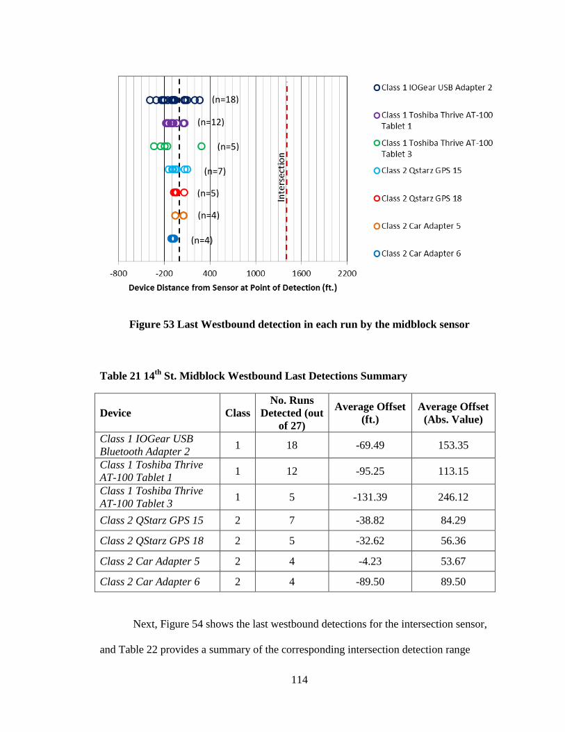
114
Figure 53 Last Westbound detection in each run by the midblock sensor
Table 21 14th
St. Midblock Westbound Last Detections Summary
Device Class
No. Runs
Detected (out
of 27)
Average Offset
(ft.)
Average Offset
(Abs. Value)
Class 1 IOGear USB
Bluetooth Adapter 2 1 18 -69.49 153.35
Class 1 Toshiba Thrive
AT-100 Tablet 1 1 12 -95.25 113.15
Class 1 Toshiba Thrive
AT-100 Tablet 3 1 5 -131.39 246.12
Class 2 QStarz GPS 15 2 7 -38.82 84.29
Class 2 QStarz GPS 18 2 5 -32.62 56.36
Class 2 Car Adapter 5 2 4 -4.23 53.67
Class 2 Car Adapter 6 2 4 -89.50 89.50
Next, Figure 54 shows the last westbound detections for the intersection sensor,
and Table 22 provides a summary of the corresponding intersection detection range
(n=18)
(n=12)
(n=5)
(n=7)
(n=5)
(n=4)
(n=4)
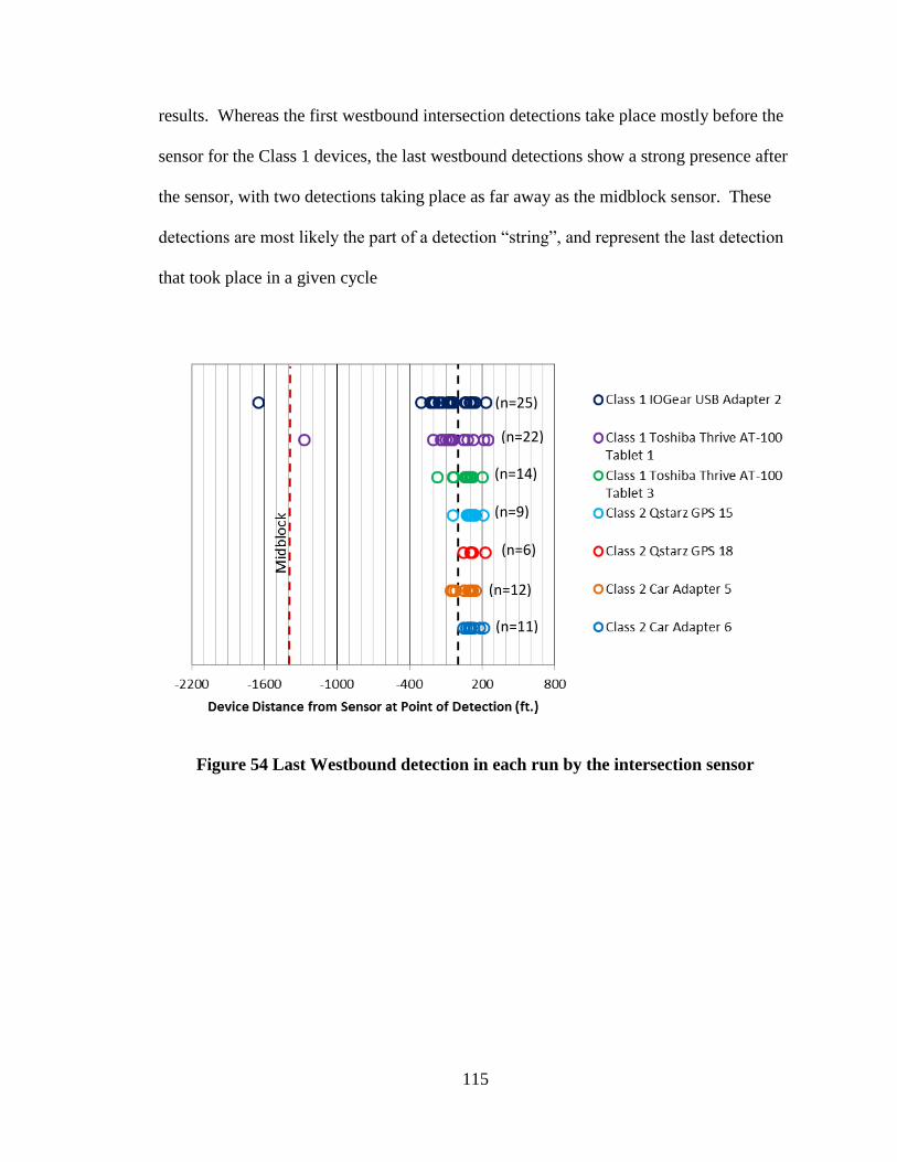
115
results. Whereas the first westbound intersection detections take place mostly before the
sensor for the Class 1 devices, the last westbound detections show a strong presence after
the sensor, with two detections taking place as far away as the midblock sensor. These
detections are most likely the part of a detection “string”, and represent the last detection
that took place in a given cycle
Figure 54 Last Westbound detection in each run by the intersection sensor
(n=25)
(n=22)
(n=14)
(n=9)
(n=6)
(n=12)
(n=11)
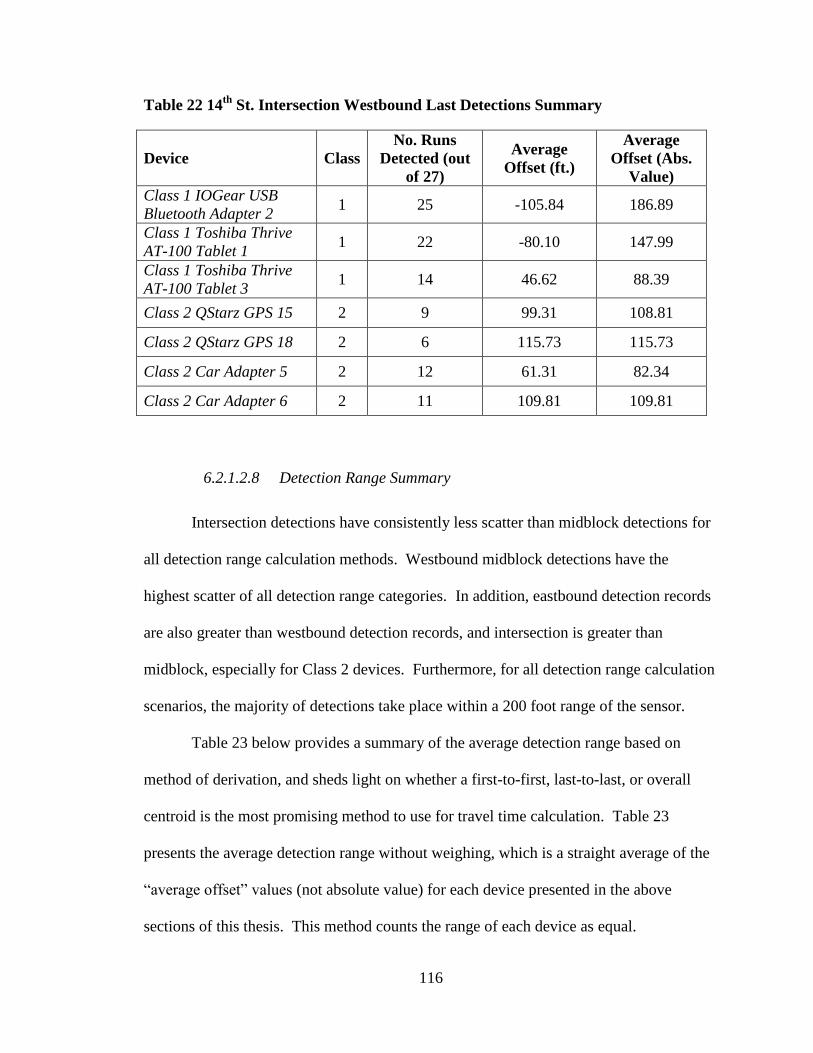
116
Table 22 14th
St. Intersection Westbound Last Detections Summary
Device Class
No. Runs
Detected (out
of 27)
Average
Offset (ft.)
Average
Offset (Abs.
Value)
Class 1 IOGear USB
Bluetooth Adapter 2 1 25 -105.84 186.89
Class 1 Toshiba Thrive
AT-100 Tablet 1 1 22 -80.10 147.99
Class 1 Toshiba Thrive
AT-100 Tablet 3 1 14 46.62 88.39
Class 2 QStarz GPS 15 2 9 99.31 108.81
Class 2 QStarz GPS 18 2 6 115.73 115.73
Class 2 Car Adapter 5 2 12 61.31 82.34
Class 2 Car Adapter 6 2 11 109.81 109.81
6.2.1.2.8 Detection Range Summary
Intersection detections have consistently less scatter than midblock detections for
all detection range calculation methods. Westbound midblock detections have the
highest scatter of all detection range categories. In addition, eastbound detection records
are also greater than westbound detection records, and intersection is greater than
midblock, especially for Class 2 devices. Furthermore, for all detection range calculation
scenarios, the majority of detections take place within a 200 foot range of the sensor.
Table 23 below provides a summary of the average detection range based on
method of derivation, and sheds light on whether a first-to-first, last-to-last, or overall
centroid is the most promising method to use for travel time calculation. Table 23
presents the average detection range without weighing, which is a straight average of the
“average offset” values (not absolute value) for each device presented in the above
sections of this thesis. This method counts the range of each device as equal.
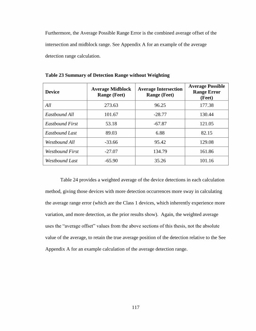
117
Furthermore, the Average Possible Range Error is the combined average offset of the
intersection and midblock range. See Appendix A for an example of the average
detection range calculation.
Table 23 Summary of Detection Range without Weighting
Device Average Midblock
Range (Feet)
Average Intersection
Range (Feet)
Average Possible
Range Error
(Feet)
All 273.63 96.25 177.38
Eastbound All 101.67 -28.77 130.44
Eastbound First 53.18 -67.87 121.05
Eastbound Last 89.03 6.88 82.15
Westbound All -33.66 95.42 129.08
Westbound First -27.07 134.79 161.86
Westbound Last -65.90 35.26 101.16
Table 24 provides a weighted average of the device detections in each calculation
method, giving those devices with more detection occurrences more sway in calculating
the average range error (which are the Class 1 devices, which inherently experience more
variation, and more detection, as the prior results show). Again, the weighted average
uses the “average offset” values from the above sections of this thesis, not the absolute
value of the average, to retain the true average position of the detection relative to the See
Appendix A for an example calculation of the average detection range.
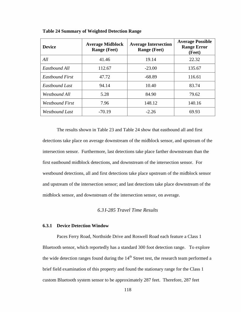
118
Table 24 Summary of Weighted Detection Range
Device Average Midblock
Range (Feet)
Average Intersection
Range (Feet)
Average Possible
Range Error
(Feet)
All 41.46 19.14 22.32
Eastbound All 112.67 -23.00 135.67
Eastbound First 47.72 -68.89 116.61
Eastbound Last 94.14 10.40 83.74
Westbound All 5.28 84.90 79.62
Westbound First 7.96 148.12 140.16
Westbound Last -70.19 -2.26 69.93
The results shown in Table 23 and Table 24 show that eastbound all and first
detections take place on average downstream of the midblock sensor, and upstream of the
intersection sensor. Furthermore, last detections take place farther downstream than the
first eastbound midblock detections, and downstream of the intersection sensor. For
westbound detections, all and first detections take place upstream of the midblock sensor
and upstream of the intersection sensor; and last detections take place downstream of the
midblock sensor, and downstream of the intersection sensor, on average.
6.3 I-285 Travel Time Results
6.3.1 Device Detection Window
Paces Ferry Road, Northside Drive and Roswell Road each feature a Class 1
Bluetooth sensor, which reportedly has a standard 300 foot detection range. To explore
the wide detection ranges found during the 14th
Street test, the research team performed a
brief field examination of this property and found the stationary range for the Class 1
custom Bluetooth system sensor to be approximately 287 feet. Therefore, 287 feet

119
defines the radius of the circle around the sensor representing the device detection
window. Each sensor has the same approximate detection radius, but because the
position of the sensor relative to the travel lanes is different at each data collection site on
I-285 eastbound, the window is slightly different for each location. An understanding of
the detection window is important because it describes the length of time a given
Bluetooth-enabled device is in a sensor’s field of view. The device does not become
detectable until crossing over this invisible threshold.
6.3.1.1 Paces Ferry Road Eastbound Detection Window
Paces Ferry Road features four eastbound and four westbound lanes of traffic,
with the Bluetooth sensor stationed on the right side of the eastbound traffic. The sensor
at Paces Ferry Road is placed approximately 15 feet from the guardrail. The shoulder
between the guardrail and the outside lane of traffic is approximately 15 feet wide. Each
lane is about 12 feet wide, and the distance from the inside lane to the middle of the
concrete barrier separating eastbound and westbound traffic is about seven feet.
Therefore, there is about 85 feet from the sensor to edge of eastbound traffic, and 140 feet
to the edge of westbound traffic.
The overpass at Paces Ferry Road, which is about 125 feet away from the sensor
location, constitutes an obstacle to communication. Table 25 below provides a
breakdown of the time a vehicle is within the Paces Ferry Road detection window by lane
and traffic speed. Refer to Appendix B for details regarding the calculation of the
detection window. Lane 0 is the inside lane, increasing as the lanes move out from the
center in either direction. The westbound congested is greyed out because the westbound
was in free-flow for the entire AM morning data collection period. Table 25 shows that

120
as the eastbound traffic experiences more congestion, the westbound traffic spends
proportionately less time in the detection window.
Table 25 Paces Ferry Road Eastbound Detection Window by Lane and Speed
Free-Flow
(65 mph)
Congested
(40 mph)
Congested
(20 mph)
Lane I.D. Distance (feet) Time (sec) Time (sec) Time (sec)
Eastbound
3 569 5.97 9.70 19.40
2 566 5.94 9.65 19.30
1 561 5.88 9.56 19.12
0 556 5.83 9.48 18.96
Westbound
0 539 5.65
1 530 5.56
2 519 5.45
3 508 5.25
6.3.1.2 Northside Drive Eastbound Detection Window
Northside Drive at I-285 features five lanes it the eastbound direction and five
lanes in the westbound direction. The same roadway dimensions are taken as in Paces
Ferry Road, with the difference lying in the sensor offset from the guardrail, which is
about five feet instead of 15 feet. Table 26 below provides a breakdown of the time a
vehicle is within the detection window by lane and traffic speed. The ratio of eastbound
to westbound time present in the detection window at Northside Drive is very close to
Paces Ferry Road. As the congestion increases, and speed decreases, the volume of
vehicles present in the detection window at any one time increases. As a result, the
presence of devices should increase.
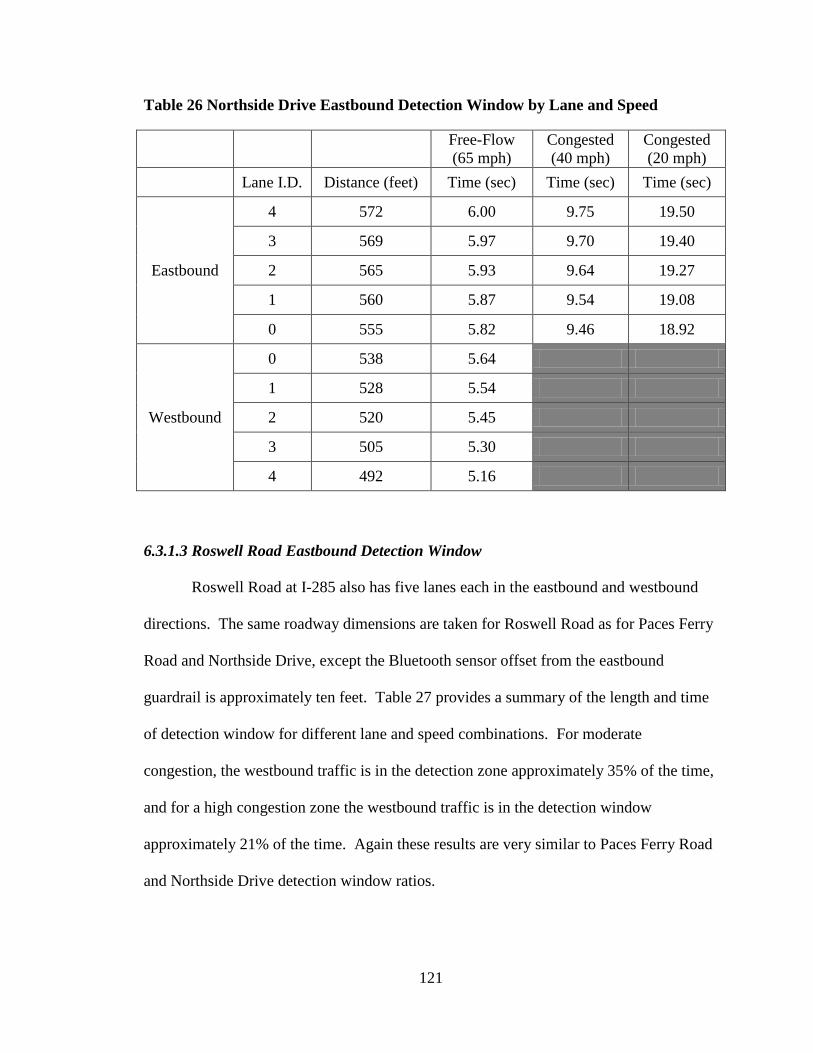
121
Table 26 Northside Drive Eastbound Detection Window by Lane and Speed
Free-Flow
(65 mph)
Congested
(40 mph)
Congested
(20 mph)
Lane I.D. Distance (feet) Time (sec) Time (sec) Time (sec)
Eastbound
4 572 6.00 9.75 19.50
3 569 5.97 9.70 19.40
2 565 5.93 9.64 19.27
1 560 5.87 9.54 19.08
0 555 5.82 9.46 18.92
Westbound
0 538 5.64
1 528 5.54
2 520 5.45
3 505 5.30
4 492 5.16
6.3.1.3 Roswell Road Eastbound Detection Window
Roswell Road at I-285 also has five lanes each in the eastbound and westbound
directions. The same roadway dimensions are taken for Roswell Road as for Paces Ferry
Road and Northside Drive, except the Bluetooth sensor offset from the eastbound
guardrail is approximately ten feet. Table 27 provides a summary of the length and time
of detection window for different lane and speed combinations. For moderate
congestion, the westbound traffic is in the detection zone approximately 35% of the time,
and for a high congestion zone the westbound traffic is in the detection window
approximately 21% of the time. Again these results are very similar to Paces Ferry Road
and Northside Drive detection window ratios.
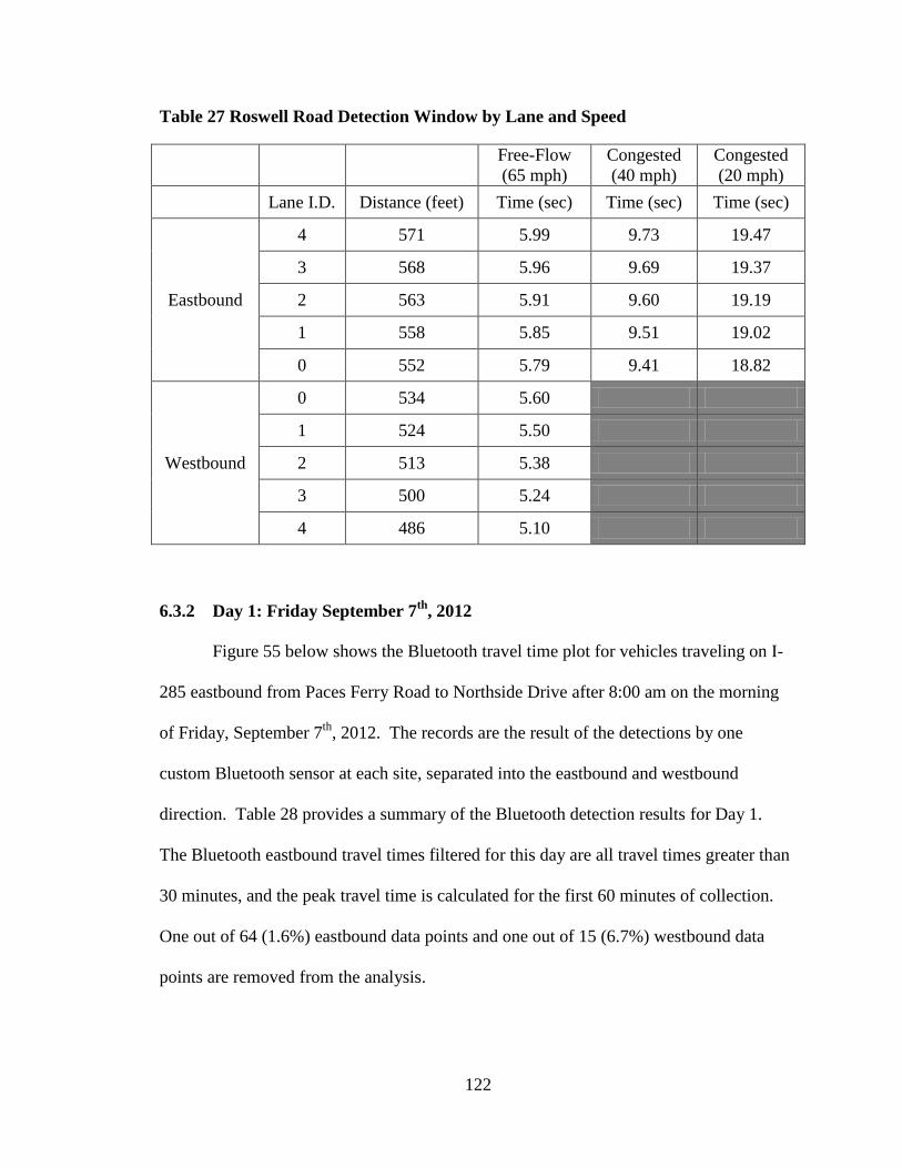
122
Table 27 Roswell Road Detection Window by Lane and Speed
Free-Flow
(65 mph)
Congested
(40 mph)
Congested
(20 mph)
Lane I.D. Distance (feet) Time (sec) Time (sec) Time (sec)
Eastbound
4 571 5.99 9.73 19.47
3 568 5.96 9.69 19.37
2 563 5.91 9.60 19.19
1 558 5.85 9.51 19.02
0 552 5.79 9.41 18.82
Westbound
0 534 5.60
1 524 5.50
2 513 5.38
3 500 5.24
4 486 5.10
6.3.2 Day 1: Friday September 7th
, 2012
Figure 55 below shows the Bluetooth travel time plot for vehicles traveling on I-
285 eastbound from Paces Ferry Road to Northside Drive after 8:00 am on the morning
of Friday, September 7th
, 2012. The records are the result of the detections by one
custom Bluetooth sensor at each site, separated into the eastbound and westbound
direction. Table 28 provides a summary of the Bluetooth detection results for Day 1.
The Bluetooth eastbound travel times filtered for this day are all travel times greater than
30 minutes, and the peak travel time is calculated for the first 60 minutes of collection.
One out of 64 (1.6%) eastbound data points and one out of 15 (6.7%) westbound data
points are removed from the analysis.
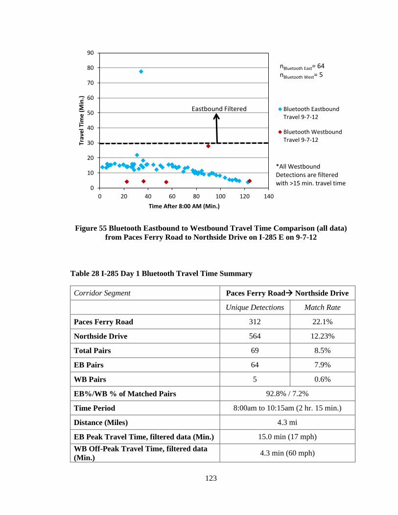
123
Figure 55 Bluetooth Eastbound to Westbound Travel Time Comparison (all data)
from Paces Ferry Road to Northside Drive on I-285 E on 9-7-12
Table 28 I-285 Day 1 Bluetooth Travel Time Summary
Corridor Segment Paces Ferry Road Northside Drive
Unique Detections Match Rate
Paces Ferry Road 312 22.1%
Northside Drive 564 12.23%
Total Pairs 69 8.5%
EB Pairs 64 7.9%
WB Pairs 5 0.6%
EB%/WB % of Matched Pairs 92.8% / 7.2%
Time Period 8:00am to 10:15am (2 hr. 15 min.)
Distance (Miles) 4.3 mi
EB Peak Travel Time, filtered data (Min.) 15.0 min (17 mph)
WB Off-Peak Travel Time, filtered data
(Min.) 4.3 min (60 mph)
0
10
20
30
40
50
60
70
80
90
0 20 40 60 80 100 120 140
Trav
el T
ime
(M
in.)
Time After 8:00 AM (Min.)
Bluetooth EastboundTravel 9-7-12
Bluetooth WestboundTravel 9-7-12
nBluetooth East= 64 nBluetooth West= 5
Eastbound Filtered
*All Westbound Detections are filtered with >15 min. travel time
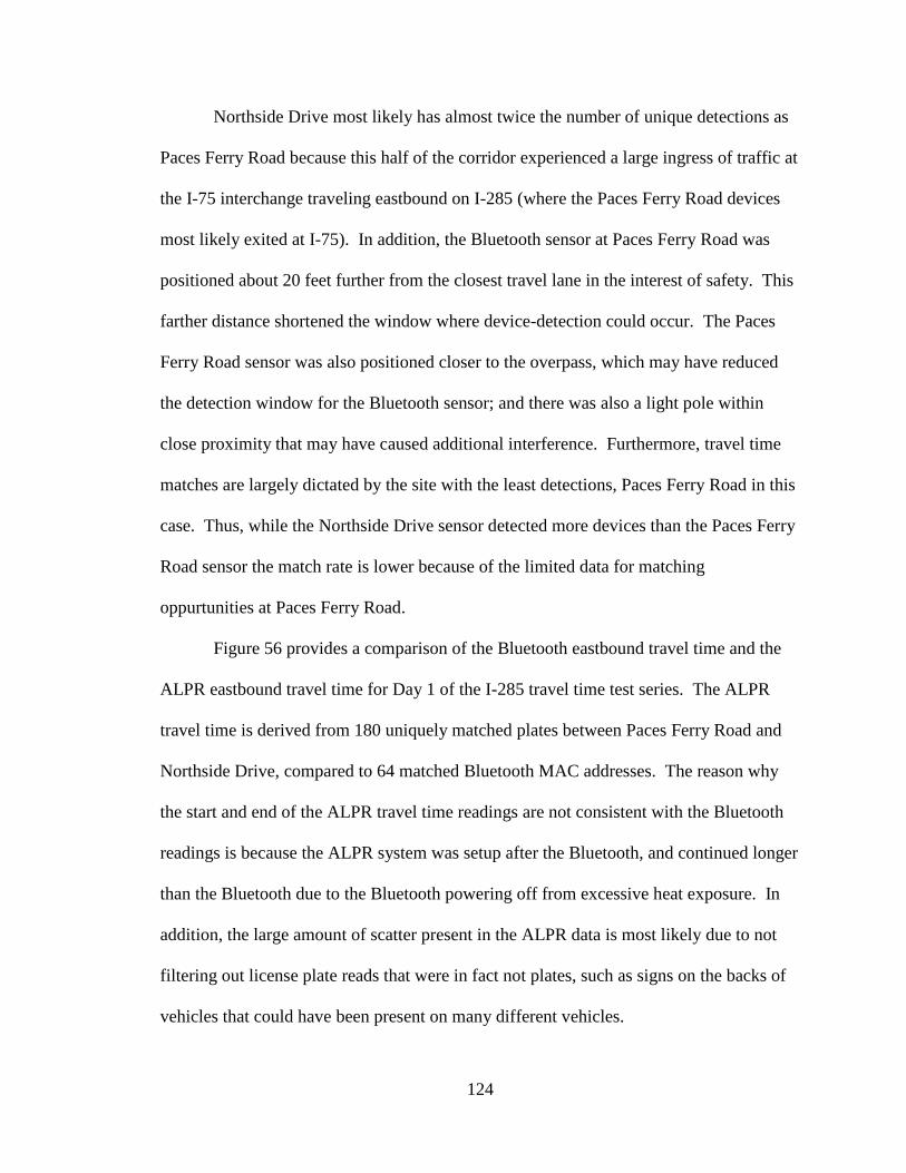
124
Northside Drive most likely has almost twice the number of unique detections as
Paces Ferry Road because this half of the corridor experienced a large ingress of traffic at
the I-75 interchange traveling eastbound on I-285 (where the Paces Ferry Road devices
most likely exited at I-75). In addition, the Bluetooth sensor at Paces Ferry Road was
positioned about 20 feet further from the closest travel lane in the interest of safety. This
farther distance shortened the window where device-detection could occur. The Paces
Ferry Road sensor was also positioned closer to the overpass, which may have reduced
the detection window for the Bluetooth sensor; and there was also a light pole within
close proximity that may have caused additional interference. Furthermore, travel time
matches are largely dictated by the site with the least detections, Paces Ferry Road in this
case. Thus, while the Northside Drive sensor detected more devices than the Paces Ferry
Road sensor the match rate is lower because of the limited data for matching
oppurtunities at Paces Ferry Road.
Figure 56 provides a comparison of the Bluetooth eastbound travel time and the
ALPR eastbound travel time for Day 1 of the I-285 travel time test series. The ALPR
travel time is derived from 180 uniquely matched plates between Paces Ferry Road and
Northside Drive, compared to 64 matched Bluetooth MAC addresses. The reason why
the start and end of the ALPR travel time readings are not consistent with the Bluetooth
readings is because the ALPR system was setup after the Bluetooth, and continued longer
than the Bluetooth due to the Bluetooth powering off from excessive heat exposure. In
addition, the large amount of scatter present in the ALPR data is most likely due to not
filtering out license plate reads that were in fact not plates, such as signs on the backs of
vehicles that could have been present on many different vehicles.

125
Figure 56 Bluetooth and ALPR Travel Time Comparison (all data) from Paces
Ferry Road to Northside Drive on I-285 E on 9-7-12
6.3.3 Day 2: Wednesday September 12th
, 2012
Figure 57 below shows the travel time from Northside Drive to Roswell Road
after 7:30 AM on Wednesday, September 12th
, 2012. The records are the result of the
detections by one custom Bluetooth sensor at each site, separated into the eastbound and
westbound direction. The westbound travel time presents a baseline for what the free-
flow non-congested travel time is for the corridor, which is 3.3 minutes. Table 29
provides a summary of the Bluetooth detection results for Day 2. The Bluetooth
eastbound travel times filtered for this day are all travel times greater than 20 minutes,
and the peak travel time is calculated for the first 30 minutes of collection. Three out of
266 (1%) eastbound points and two out of 15 (13%) westbound points are removed.
0
20
40
60
80
100
120
0 20 40 60 80 100 120 140 160
Trav
el T
ime
(M
in.)
Time After 8:00 AM (Min.)
ALPR EastboundTravel 9-7-12
Bluetooth EastboundTravel 9-7-12
nBluetooth East = 64 nALPR East = 180
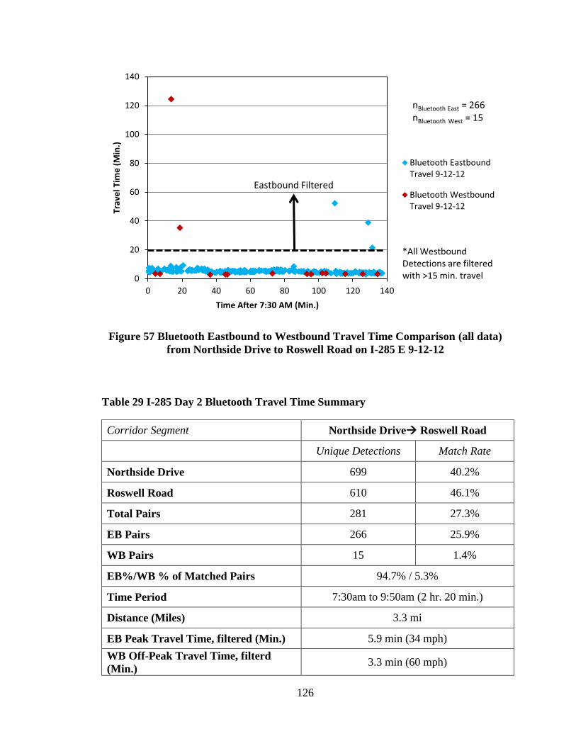
126
Figure 57 Bluetooth Eastbound to Westbound Travel Time Comparison (all data)
from Northside Drive to Roswell Road on I-285 E 9-12-12
Table 29 I-285 Day 2 Bluetooth Travel Time Summary
Corridor Segment Northside Drive Roswell Road
Unique Detections Match Rate
Northside Drive 699 40.2%
Roswell Road 610 46.1%
Total Pairs 281 27.3%
EB Pairs 266 25.9%
WB Pairs 15 1.4%
EB%/WB % of Matched Pairs 94.7% / 5.3%
Time Period 7:30am to 9:50am (2 hr. 20 min.)
Distance (Miles) 3.3 mi
EB Peak Travel Time, filtered (Min.) 5.9 min (34 mph)
WB Off-Peak Travel Time, filterd
(Min.) 3.3 min (60 mph)
0
20
40
60
80
100
120
140
0 20 40 60 80 100 120 140
Trav
el T
ime
(M
in.)
Time After 7:30 AM (Min.)
Bluetooth EastboundTravel 9-12-12
Bluetooth WestboundTravel 9-12-12
nBluetooth East = 266 nBluetooth West = 15
Eastbound Filtered
*All Westbound Detections are filtered with >15 min. travel
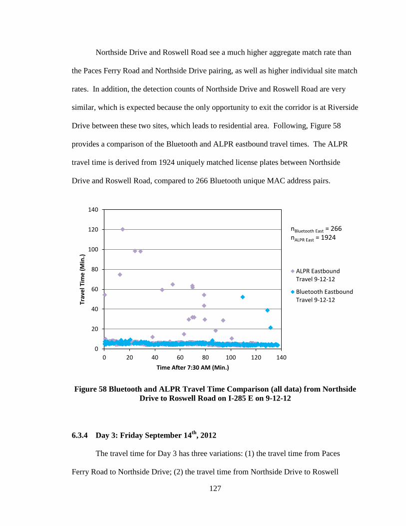
127
Northside Drive and Roswell Road see a much higher aggregate match rate than
the Paces Ferry Road and Northside Drive pairing, as well as higher individual site match
rates. In addition, the detection counts of Northside Drive and Roswell Road are very
similar, which is expected because the only opportunity to exit the corridor is at Riverside
Drive between these two sites, which leads to residential area. Following, Figure 58
provides a comparison of the Bluetooth and ALPR eastbound travel times. The ALPR
travel time is derived from 1924 uniquely matched license plates between Northside
Drive and Roswell Road, compared to 266 Bluetooth unique MAC address pairs.
Figure 58 Bluetooth and ALPR Travel Time Comparison (all data) from Northside
Drive to Roswell Road on I-285 E on 9-12-12
6.3.4 Day 3: Friday September 14th
, 2012
The travel time for Day 3 has three variations: (1) the travel time from Paces
Ferry Road to Northside Drive; (2) the travel time from Northside Drive to Roswell
0
20
40
60
80
100
120
140
0 20 40 60 80 100 120 140
Trav
el T
ime
(M
in.)
Time After 7:30 AM (Min.)
ALPR EastboundTravel 9-12-12
Bluetooth EastboundTravel 9-12-12
nBluetooth East = 266 nALPR East = 1924

128
Road; and (3) the travel time from Paces Ferry Road to Roswell Road. The reason for
showing the travel times in these segments is to show how the entire corridor travel time
compares to the travel time along sections of the corridor.
6.3.4.1 Paces Ferry Road to Roswell Road
Figure 59 below shows the travel time from Paces Ferry Road to Roswell Road,
again captured by one custom Bluetooth sensor at each site, for the time after 7:20 AM
on Friday, September 14th
, 2012. The records separated into the eastbound and
westbound direction. The Bluetooth eastbound travel times filtered for this day are all
travel times greater than 20 minutes, and the peak travel time is calculated for times 40
minutes through 80 minutes after the start of the data collection period. Therefore, three
out of 89 eastbound data points are removed, leaving 97% of the eastbound data points
for travel time calculation. Conversely, two out of 11 westbound data points are
removed, leaving 82% of the westbound data points for travel time calculation.

129
Figure 59 Bluetooth Eastbound to Westbound Travel Time Comparison (all data)
from Paces Ferry Road to Roswell Road on I-285 E on 9-14-12
6.3.4.2 Paces Ferry Road to Northside Drive
Figure 60 shows the travel time from Paces Ferry Road to Northside Drive
captured by one Bluetooth sensor after 7:20 AM on Friday, September 14, 2012. The
records are the result of the detections by one Bluetooth sensor at each site, separated into
the eastbound and westbound direction. The number of unique MAC addressed matches
is greater for this day than Day 1 of the I-285 travel time test series. The Bluetooth
eastbound travel times filtered for this day are all travel times greater than 20 minutes,
and the peak travel time is calculated for times 40 minutes through 80 minutes after the
start of the data collection period. Therefore, five out of 95 (5.3%) eastbound data points
and two out of 11 (18.1%) westbound data points are removed out of the travel time
calculation.
0
10
20
30
40
50
60
70
0 20 40 60 80 100 120 140
Trav
el T
ime
(M
in.)
Time after 7:20 AM (Min.)
Bluetooth EastboundTravel 9-14-12
Bluetooth WestboundTravel 9-14-12
nBluetooth East = 89 nBluetooth West =11
Eastbound Filtered
*All Westbound Detections are filtered with >15 min. travel time
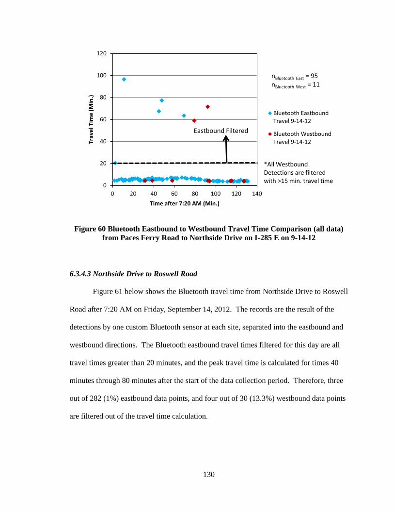
130
Figure 60 Bluetooth Eastbound to Westbound Travel Time Comparison (all data)
from Paces Ferry Road to Northside Drive on I-285 E on 9-14-12
6.3.4.3 Northside Drive to Roswell Road
Figure 61 below shows the Bluetooth travel time from Northside Drive to Roswell
Road after 7:20 AM on Friday, September 14, 2012. The records are the result of the
detections by one custom Bluetooth sensor at each site, separated into the eastbound and
westbound directions. The Bluetooth eastbound travel times filtered for this day are all
travel times greater than 20 minutes, and the peak travel time is calculated for times 40
minutes through 80 minutes after the start of the data collection period. Therefore, three
out of 282 (1%) eastbound data points, and four out of 30 (13.3%) westbound data points
are filtered out of the travel time calculation.
0
20
40
60
80
100
120
0 20 40 60 80 100 120 140
Trav
el T
ime
(M
in.)
Time after 7:20 AM (Min.)
Bluetooth EastboundTravel 9-14-12
Bluetooth WestboundTravel 9-14-12
nBluetooth East = 95 nBluetooth West = 11
Eastbound Filtered
*All Westbound Detections are filtered with >15 min. travel time
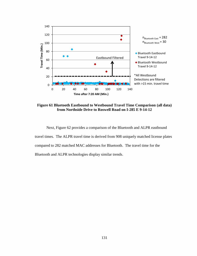
131
Figure 61 Bluetooth Eastbound to Westbound Travel Time Comparison (all data)
from Northside Drive to Roswell Road on I-285 E 9-14-12
Next, Figure 62 provides a comparison of the Bluetooth and ALPR eastbound
travel times. The ALPR travel time is derived from 908 uniquely matched license plates
compared to 282 matched MAC addresses for Bluetooth. The travel time for the
Bluetooth and ALPR technologies display similar trends.
0
20
40
60
80
100
120
140
0 20 40 60 80 100 120 140
Trav
el T
ime
(M
in.)
Time after 7:20 AM (Min.)
Bluetooth EastboundTravel 9-14-12
Bluetooth WestboundTravel 9-14-12
nBluetooth East = 282 nBluetooth West = 30
Eastbound Filtered
*All Westbound Detections are filtered with >15 min. travel time
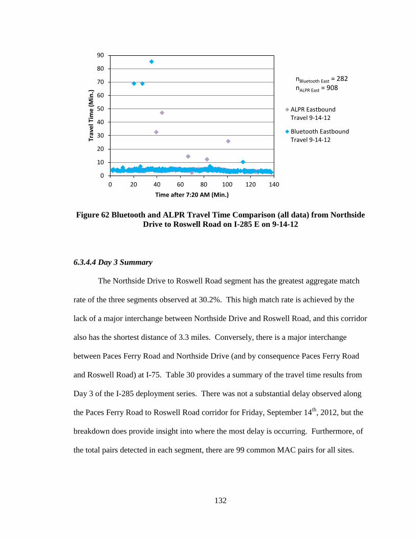
132
Figure 62 Bluetooth and ALPR Travel Time Comparison (all data) from Northside
Drive to Roswell Road on I-285 E on 9-14-12
6.3.4.4 Day 3 Summary
The Northside Drive to Roswell Road segment has the greatest aggregate match
rate of the three segments observed at 30.2%. This high match rate is achieved by the
lack of a major interchange between Northside Drive and Roswell Road, and this corridor
also has the shortest distance of 3.3 miles. Conversely, there is a major interchange
between Paces Ferry Road and Northside Drive (and by consequence Paces Ferry Road
and Roswell Road) at I-75. Table 30 provides a summary of the travel time results from
Day 3 of the I-285 deployment series. There was not a substantial delay observed along
the Paces Ferry Road to Roswell Road corridor for Friday, September 14th
, 2012, but the
breakdown does provide insight into where the most delay is occurring. Furthermore, of
the total pairs detected in each segment, there are 99 common MAC pairs for all sites.
0
10
20
30
40
50
60
70
80
90
0 20 40 60 80 100 120 140
Trav
el T
ime
(M
in.)
Time after 7:20 AM (Min.)
ALPR EastboundTravel 9-14-12
Bluetooth EastboundTravel 9-14-12
nBluetooth East = 282 nALPR East = 908
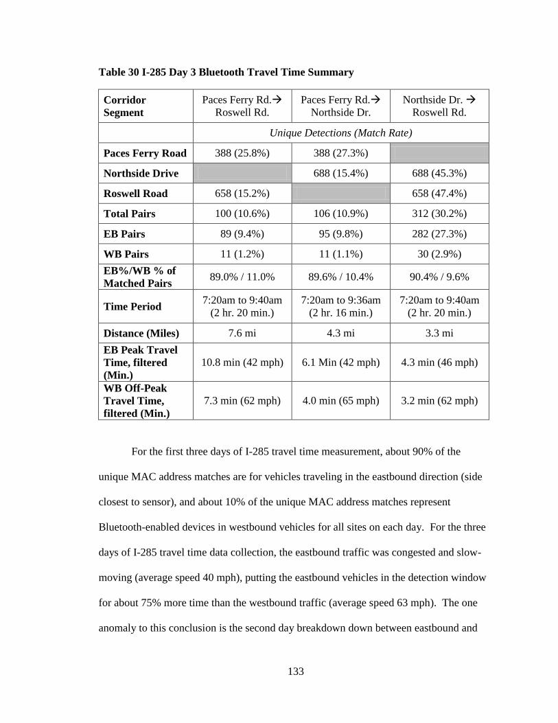
133
Table 30 I-285 Day 3 Bluetooth Travel Time Summary
Corridor
Segment
Paces Ferry Rd.
Roswell Rd.
Paces Ferry Rd.
Northside Dr.
Northside Dr.
Roswell Rd.
Unique Detections (Match Rate)
Paces Ferry Road 388 (25.8%) 388 (27.3%)
Northside Drive 688 (15.4%) 688 (45.3%)
Roswell Road 658 (15.2%) 658 (47.4%)
Total Pairs 100 (10.6%) 106 (10.9%) 312 (30.2%)
EB Pairs 89 (9.4%) 95 (9.8%) 282 (27.3%)
WB Pairs 11 (1.2%) 11 (1.1%) 30 (2.9%)
EB%/WB % of
Matched Pairs 89.0% / 11.0% 89.6% / 10.4% 90.4% / 9.6%
Time Period 7:20am to 9:40am
(2 hr. 20 min.)
7:20am to 9:36am
(2 hr. 16 min.)
7:20am to 9:40am
(2 hr. 20 min.)
Distance (Miles) 7.6 mi 4.3 mi 3.3 mi
EB Peak Travel
Time, filtered
(Min.)
10.8 min (42 mph) 6.1 Min (42 mph) 4.3 min (46 mph)
WB Off-Peak
Travel Time,
filtered (Min.)
7.3 min (62 mph) 4.0 min (65 mph) 3.2 min (62 mph)
For the first three days of I-285 travel time measurement, about 90% of the
unique MAC address matches are for vehicles traveling in the eastbound direction (side
closest to sensor), and about 10% of the unique MAC address matches represent
Bluetooth-enabled devices in westbound vehicles for all sites on each day. For the three
days of I-285 travel time data collection, the eastbound traffic was congested and slow-
moving (average speed 40 mph), putting the eastbound vehicles in the detection window
for about 75% more time than the westbound traffic (average speed 63 mph). The one
anomaly to this conclusion is the second day breakdown down between eastbound and
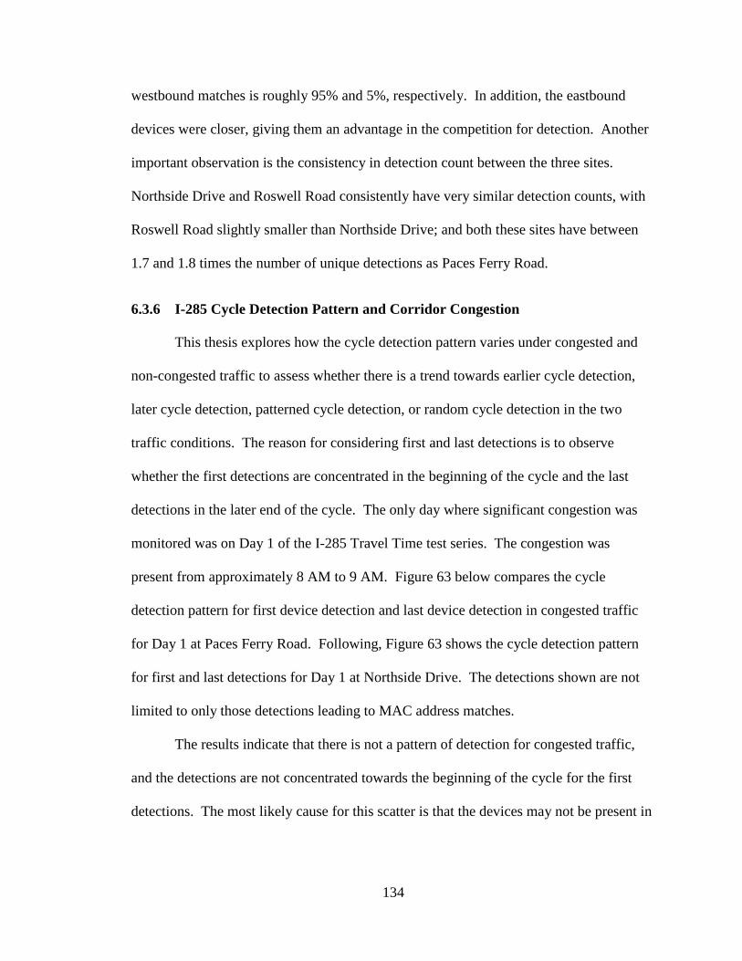
134
westbound matches is roughly 95% and 5%, respectively. In addition, the eastbound
devices were closer, giving them an advantage in the competition for detection. Another
important observation is the consistency in detection count between the three sites.
Northside Drive and Roswell Road consistently have very similar detection counts, with
Roswell Road slightly smaller than Northside Drive; and both these sites have between
1.7 and 1.8 times the number of unique detections as Paces Ferry Road.
6.3.6 I-285 Cycle Detection Pattern and Corridor Congestion
This thesis explores how the cycle detection pattern varies under congested and
non-congested traffic to assess whether there is a trend towards earlier cycle detection,
later cycle detection, patterned cycle detection, or random cycle detection in the two
traffic conditions. The reason for considering first and last detections is to observe
whether the first detections are concentrated in the beginning of the cycle and the last
detections in the later end of the cycle. The only day where significant congestion was
monitored was on Day 1 of the I-285 Travel Time test series. The congestion was
present from approximately 8 AM to 9 AM. Figure 63 below compares the cycle
detection pattern for first device detection and last device detection in congested traffic
for Day 1 at Paces Ferry Road. Following, Figure 63 shows the cycle detection pattern
for first and last detections for Day 1 at Northside Drive. The detections shown are not
limited to only those detections leading to MAC address matches.
The results indicate that there is not a pattern of detection for congested traffic,
and the detections are not concentrated towards the beginning of the cycle for the first
detections. The most likely cause for this scatter is that the devices may not be present in
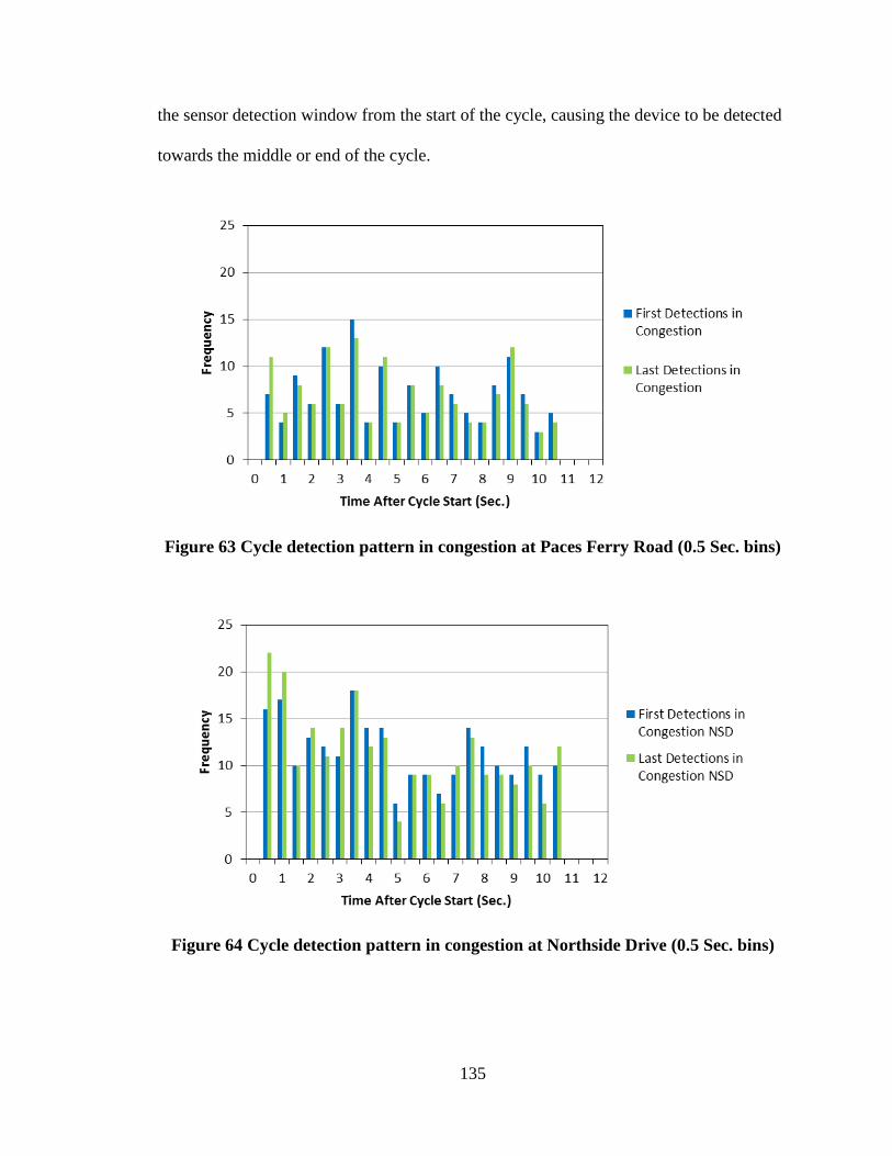
135
the sensor detection window from the start of the cycle, causing the device to be detected
towards the middle or end of the cycle.
Figure 63 Cycle detection pattern in congestion at Paces Ferry Road (0.5 Sec. bins)
Figure 64 Cycle detection pattern in congestion at Northside Drive (0.5 Sec. bins)
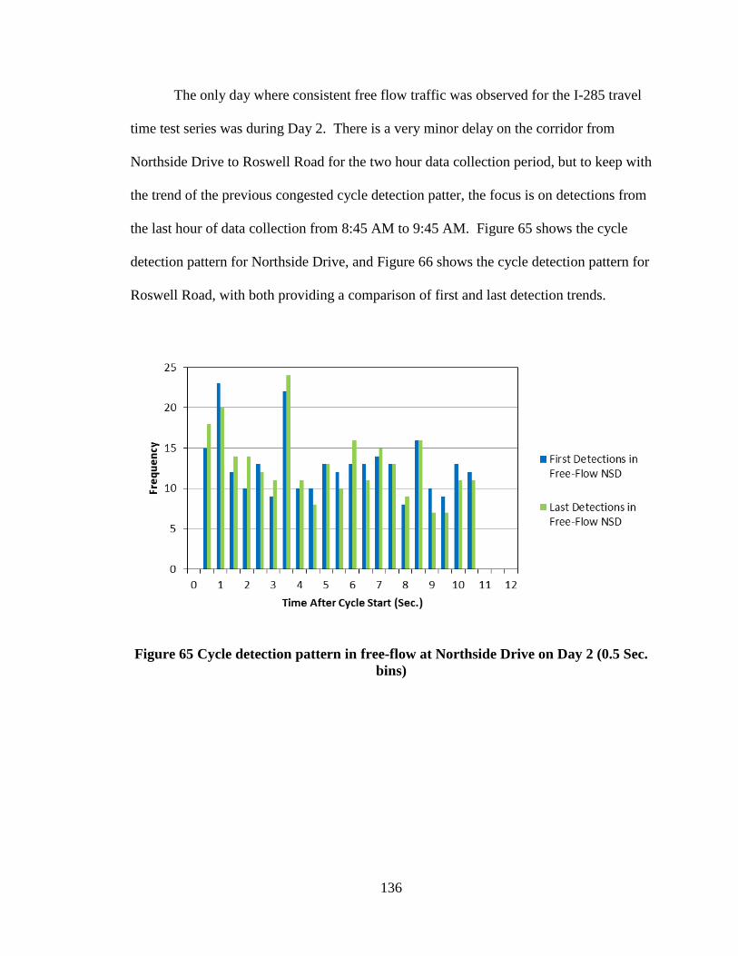
136
The only day where consistent free flow traffic was observed for the I-285 travel
time test series was during Day 2. There is a very minor delay on the corridor from
Northside Drive to Roswell Road for the two hour data collection period, but to keep with
the trend of the previous congested cycle detection patter, the focus is on detections from
the last hour of data collection from 8:45 AM to 9:45 AM. Figure 65 shows the cycle
detection pattern for Northside Drive, and Figure 66 shows the cycle detection pattern for
Roswell Road, with both providing a comparison of first and last detection trends.
Figure 65 Cycle detection pattern in free-flow at Northside Drive on Day 2 (0.5 Sec.
bins)

137
Figure 66 Cycle detection pattern in free-flow for Roswell Road on Day 2 (0.5 Sec.
bins)
Just as for the congested traffic, there does not seem to be a concentration of
detections towards the beginning of the cycle for the first detections in free flow traffic.
Rather, the last detections are showing a higher concentration in the beginning of the
cycle than the first detections for Northside Drive and Roswell Road. These results show
that an inquiry cycle length of 10.24 seconds is sufficient to capture the discoverable
devices in the vehicle population, because there is no unused time where detections are
not occurring throughout the cycle duration.
6.4 I-285Work Zone Travel Time Results
6.4.1 Day 1: Saturday September 29, 2012
Figure 67 below shows the travel time from Riverside Drive to Paces Ferry Road
for time after 7:14 AM on Saturday, September 29, 2012. The records are the result of
the detections by one Bluetooth sensor placed on the right side of westbound traffic at
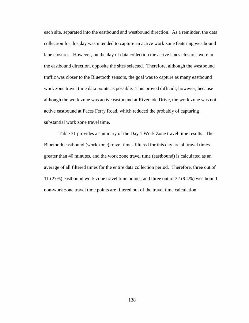
138
each site, separated into the eastbound and westbound direction. As a reminder, the data
collection for this day was intended to capture an active work zone featuring westbound
lane closures. However, on the day of data collection the active lanes closures were in
the eastbound direction, opposite the sites selected. Therefore, although the westbound
traffic was closer to the Bluetooth sensors, the goal was to capture as many eastbound
work zone travel time data points as possible. This proved difficult, however, because
although the work zone was active eastbound at Riverside Drive, the work zone was not
active eastbound at Paces Ferry Road, which reduced the probably of capturing
substantial work zone travel time.
Table 31 provides a summary of the Day 1 Work Zone travel time results. The
Bluetooth eastbound (work zone) travel times filtered for this day are all travel times
greater than 40 minutes, and the work zone travel time (eastbound) is calculated as an
average of all filtered times for the entire data collection period. Therefore, three out of
11 (27%) eastbound work zone travel time points, and three out of 32 (9.4%) westbound
non-work zone travel time points are filtered out of the travel time calculation.
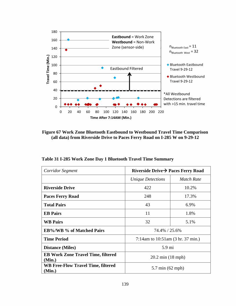
139
Figure 67 Work Zone Bluetooth Eastbound to Westbound Travel Time Comparison
(all data) from Riverside Drive to Paces Ferry Road on I-285 W on 9-29-12
Table 31 I-285 Work Zone Day 1 Bluetooth Travel Time Summary
Corridor Segment Riverside Drive Paces Ferry Road
Unique Detections Match Rate
Riverside Drive 422 10.2%
Paces Ferry Road 248 17.3%
Total Pairs 43 6.9%
EB Pairs 11 1.8%
WB Pairs 32 5.1%
EB%/WB % of Matched Pairs 74.4% / 25.6%
Time Period 7:14am to 10:51am (3 hr. 37 min.)
Distance (Miles) 5.9 mi
EB Work Zone Travel Time, filtered
(Min.) 20.2 min (18 mph)
WB Free-Flow Travel Time, filtered
(Min.) 5.7 min (62 mph)
0
20
40
60
80
100
120
140
160
180
0 20 40 60 80 100 120 140 160 180 200 220
Trav
el T
ime
(M
in.)
Time After 7:14AM (Min.)
Bluetooth EastboundTravel 9-29-12
Bluetooth WestboundTravel 9-29-12
nBluetooth East = 11
nBluetooth West = 32
Eastbound Filtered
*All Westbound Detections are filtered with >15 min. travel time
Eastbound = Work Zone Westbound = Non-Work Zone (sensor-side)
140
For the first day of intended work zone travel time capture, the westbound devices
account for approximately 75% of unique MAC address matches (side closest to sensor),
and the eastbound for 25% of unique MAC address matches. For the first day of
attempted work zone data collection, the westbound traffic (sensor side) was more sparse
and moving more quickly (about 63 mph) than the eastbound traffic at Riverside Drive
(about 18 mph); but at Paces Ferry Road the eastbound and westbound traffic was equally
sparse and in free-flow (about 63 mph). This places the eastbound traffic in the detection
window for about 3.5 times the westbound traffic time at Riverside Drive, but the amount
of shared window time was comparable for eastbound and westbound at Paces Ferry
Road. Therefore, because of the free-flow at Paces Ferry Road eastbound, the potential
for collecting downstream work zone travel time was reduced. This outcome is evident
in the preceding results.
Next, Figure 68 shows the travel time derived from the ALPR system detection
records. These travel time records very closely mirror the travel time trend from the
Bluetooth sensors, and consist of 90 unique license plate matches for vehicles traveling in
the westbound direction, compared to 32 matched Bluetooth MAC addresses.

141
Figure 68 Bluetooth and ALPR Travel Time Comparison (all data) from Riverside
Drive to Paces Ferry Road on I-285 W on 9-29-12
6.4.2 Day 2: Saturday October 20, 2012
Figure 69 below shows the Bluetooth work zone travel time measured by one
custom sensor at eastbound Paces Ferry Road and Northside Drive for the time after 9:25
AM on Saturday, October 20, 2012. The travel time is separated into the eastbound and
westbound directions. The active lane closures were present in the eastbound direction,
so the Bluetooth sensors were able to directly capture the work zone travel time during
this day of data collection. Table 32 provides a summary of the travel time statistics for
the second day of active work zone data collection. There is no base filtering for this day
of data collection because no extreme travel time values are present for the eastbound or
westbound directions; and the work zone Bluetooth travel time is calculated as an
average of all eastbound travel times for the entire data collection period.
0
20
40
60
80
100
120
140
160
180
0 20 40 60 80 100 120 140 160 180 200 220
Trav
el T
ime
(M
in.)
Time After 7:14AM (Min.)
ALPR WestboundTravel 9-29-12
Bluetooth WestboundTravel 9-29-12
nBluetooth West = 32 nALPR West = 90
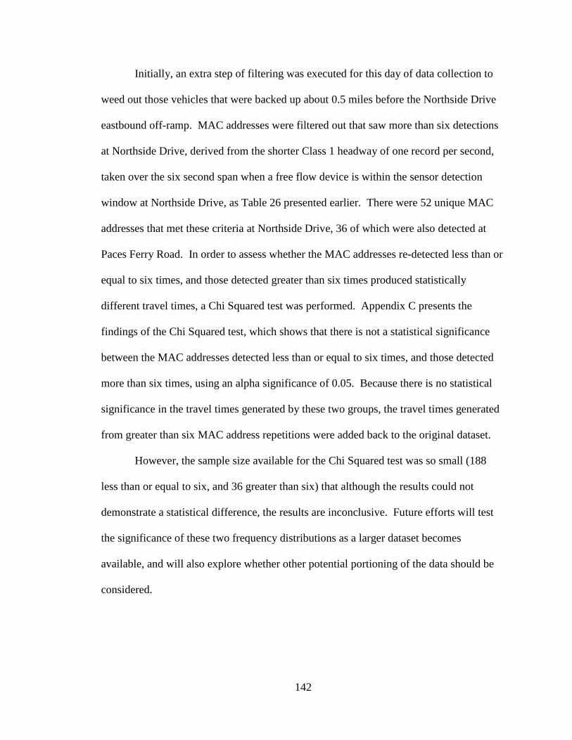
142
Initially, an extra step of filtering was executed for this day of data collection to
weed out those vehicles that were backed up about 0.5 miles before the Northside Drive
eastbound off-ramp. MAC addresses were filtered out that saw more than six detections
at Northside Drive, derived from the shorter Class 1 headway of one record per second,
taken over the six second span when a free flow device is within the sensor detection
window at Northside Drive, as Table 26 presented earlier. There were 52 unique MAC
addresses that met these criteria at Northside Drive, 36 of which were also detected at
Paces Ferry Road. In order to assess whether the MAC addresses re-detected less than or
equal to six times, and those detected greater than six times produced statistically
different travel times, a Chi Squared test was performed. Appendix C presents the
findings of the Chi Squared test, which shows that there is not a statistical significance
between the MAC addresses detected less than or equal to six times, and those detected
more than six times, using an alpha significance of 0.05. Because there is no statistical
significance in the travel times generated by these two groups, the travel times generated
from greater than six MAC address repetitions were added back to the original dataset.
However, the sample size available for the Chi Squared test was so small (188
less than or equal to six, and 36 greater than six) that although the results could not
demonstrate a statistical difference, the results are inconclusive. Future efforts will test
the significance of these two frequency distributions as a larger dataset becomes
available, and will also explore whether other potential portioning of the data should be
considered.
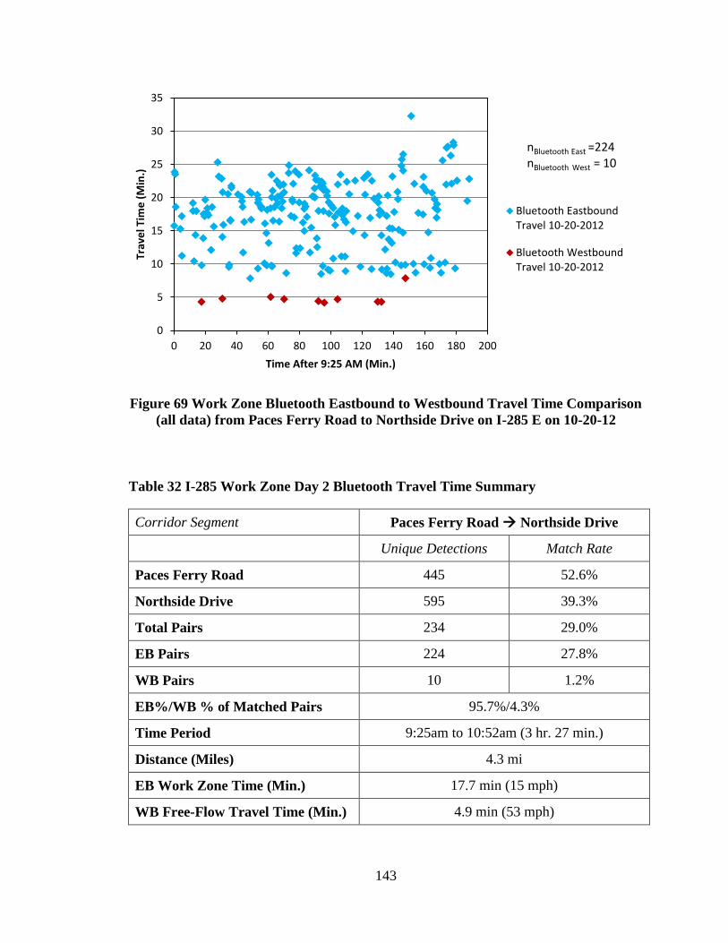
143
Figure 69 Work Zone Bluetooth Eastbound to Westbound Travel Time Comparison
(all data) from Paces Ferry Road to Northside Drive on I-285 E on 10-20-12
Table 32 I-285 Work Zone Day 2 Bluetooth Travel Time Summary
Corridor Segment Paces Ferry Road Northside Drive
Unique Detections Match Rate
Paces Ferry Road 445 52.6%
Northside Drive 595 39.3%
Total Pairs 234 29.0%
EB Pairs 224 27.8%
WB Pairs 10 1.2%
EB%/WB % of Matched Pairs 95.7%/4.3%
Time Period 9:25am to 10:52am (3 hr. 27 min.)
Distance (Miles) 4.3 mi
EB Work Zone Time (Min.) 17.7 min (15 mph)
WB Free-Flow Travel Time (Min.) 4.9 min (53 mph)
0
5
10
15
20
25
30
35
0 20 40 60 80 100 120 140 160 180 200
Trav
el T
ime
(M
in.)
Time After 9:25 AM (Min.)
Bluetooth EastboundTravel 10-20-2012
Bluetooth WestboundTravel 10-20-2012
nBluetooth East =224 nBluetooth West = 10

144
For the second day of work zone data collection, eastbound devices account for
approximately 95% of unique MAC address matches (side closest to sensor), and the
westbound for 5% of unique MAC addresses matches. The Paces Ferry Road eastbound
traffic was stop and go in significant congestion, and the Northside Drive off-ramp
eastbound was stop and go in significant congestion (despite the Northside Drive I-285
corridor traveling in free flow). Furthermore, the westbound traffic at each site was in
free flow. This presents a huge advantage for eastbound detection over westbound
detection, which the results portray.
Figure 70 below shows the eastbound ALPR travel times, derived from 203 exact
plate matches, compared to the eastbound Bluetooth travel times, derived from 224
unique MAC address matches. It appears that work zones have an inherently variable
travel time. Both the Bluetooth and ALPR data show an average travel time of 17.7
minutes in the work zone corridor.
The results also show what appears as a bimodal travel time, with a strong
presence of a ten minute travel time, as well as a 15 to 20 minute travel time for the entire
data collection period as measured by the Bluetooth sensors. The ALPR reads have no
data points in the ten minute travel time, but only in the average 17.7 minute travel time.
One possible explanation for this is that those vehicles with a ten minute travel time were
present in the left-most lane, or outside lanes, in the start of the work zone, and were not
caught into congestion until the end of the construction taper. The ALPR cameras are
less likely to detect plates in the outside lanes if there are vehicles in the inside lanes
blocking the view of the cameras. However, Bluetooth can detect devices in all lanes.
Further investigation is required to determine what lanes the vehicles were in when
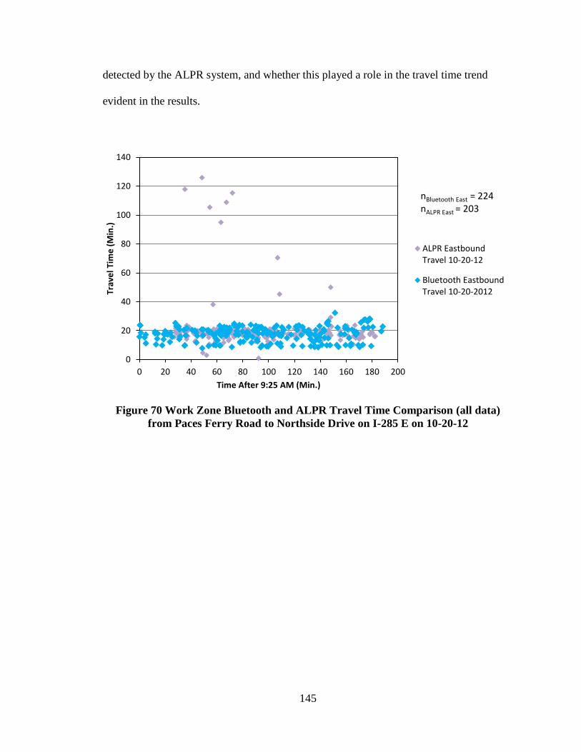
145
detected by the ALPR system, and whether this played a role in the travel time trend
evident in the results.
Figure 70 Work Zone Bluetooth and ALPR Travel Time Comparison (all data)
from Paces Ferry Road to Northside Drive on I-285 E on 10-20-12
0
20
40
60
80
100
120
140
0 20 40 60 80 100 120 140 160 180 200
Trav
el T
ime
(M
in.)
Time After 9:25 AM (Min.)
ALPR EastboundTravel 10-20-12
Bluetooth EastboundTravel 10-20-2012
nBluetooth East = 224 nALPR East = 203

146
Chapter 7: Conclusions
7.1 Discussion of Results
The findings presented in this thesis provide additional insight into the
performance of Bluetooth-enabled devices as well as Bluetooth sensors in various
controlled and uncontrolled environments. The controlled indoor tests of Bluetooth
device and sensor characteristics shed light on the unique detection properties of Class 1
and Class 2 Bluetooth enabled devices, and how those patterns of detection change with
the introduction of multiple Bluetooth sensors. The 14th
Street tests allowed the research
team to measure the average detection range of various Class 1 and Class 2 devices
around both a midblock and intersection sensor, but further statistical analysis is needed
to translate this detection range into a travel time error. The non-work zone travel time
tests on I-285 demonstrated that side-fire Bluetooth sensors provide an accurate measure
of corridor travel time, and the active work zone travel time tests reinforced this finding.
The following sections provide a brief discussion of the results presented in this thesis,
and how the findings show that Bluetooth technology is a reliable method of real-time
work zone travel time.
7.1.1 Detection Range Summary
The detection range test results show that Class 1 devices have more detection per
run, a greater detection range, greater variability in their detection location, and are
distributed both upstream and downstream of the Bluetooth sensors for all detection
range calculation methods. Class 2 devices typically have fewer detections per run (one
detection per run at the midblock location, often no detection) than Class 1 devices; less
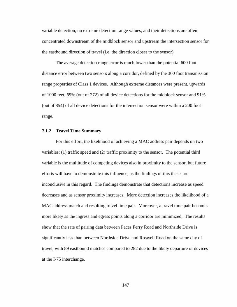
147
variable detection, no extreme detection range values, and their detections are often
concentrated downstream of the midblock sensor and upstream the intersection sensor for
the eastbound direction of travel (i.e. the direction closer to the sensor).
The average detection range error is much lower than the potential 600 foot
distance error between two sensors along a corridor, defined by the 300 foot transmission
range properties of Class 1 devices. Although extreme distances were present, upwards
of 1000 feet, 69% (out of 272) of all device detections for the midblock sensor and 91%
(out of 854) of all device detections for the intersection sensor were within a 200 foot
range.
7.1.2 Travel Time Summary
For this effort, the likelihood of achieving a MAC address pair depends on two
variables: (1) traffic speed and (2) traffic proximity to the sensor. The potential third
variable is the multitude of competing devices also in proximity to the sensor, but future
efforts will have to demonstrate this influence, as the findings of this thesis are
inconclusive in this regard. The findings demonstrate that detections increase as speed
decreases and as sensor proximity increases. More detection increases the likelihood of a
MAC address match and resulting travel time pair. Moreover, a travel time pair becomes
more likely as the ingress and egress points along a corridor are minimized. The results
show that the rate of pairing data between Paces Ferry Road and Northside Drive is
significantly less than between Northside Drive and Roswell Road on the same day of
travel, with 89 eastbound matches compared to 282 due to the likely departure of devices
at the I-75 interchange.
148
An additional factor influencing travel time generation is that the sensors may not
detect all devices within range. One reason for this lack of detection is because a device
enters and exits a sensor’s detection window before detection can occur (i.e. the device is
not present in the sensor’s detection window for the entire sensor cycle duration). The
lack of sufficient capacity for detection is likely not the cause of a missed detection,
because the results find that fifty devices, composed for 25 Class 1 and 25 Class 2
devices, do not reach the level of saturation of a single Bluetooth sensor.
7.2 Limitations of Research Study
The research team encountered several obstacles when designing the research to
meet the ultimate goal of this thesis, which was to provide a method of measuring real-
time travel time in an active work zone. The main factors that limited the scope of this
study are the personnel requirements associated with multiple Bluetooth sensor stations,
and the safe access to ideal deployment locations. The following sections detail how
these factors specifically influenced the scope of the research conducted for this thesis.
7.2.1 Personnel Requirements
Access to an adequate number of research assistants places a constraint on
acquiring an optimal number of deployment locations. About three individuals are
needed to provide adequate staff support to each site and assist with the setup and
takedown of the Bluetooth equipment. The average number of URA available for each
day of deployment was about six, which is just enough for two Bluetooth stations, in
addition to the GRA leaders. Two stations are not ideal for a large scale deployment to
cover a 15 mile work zone corridor. About six stations, or one every three miles plus one
at the end of the corridor, would have been sufficient to provide a real-time corridor
149
travel time, and capture vehicles before and after major egress and ingress points along
the corridor. In addition to the limited number of available URAs for each day of data
collection, the number of trained GRAs was always either two or three. One GRA is
required at each data collection site to oversee the equipment setup, and ensure that the
data collection proceeds safely and according to schedule. The limit of properly trained
GRAs put an additional constraint on deploying at the optimal number of sites. While
some of these constraints are specific to the research environment, it is expected that a
regular field implementation of Bluetooth equipment will require additional personnel
requirements, in terms of man-hours and training, in roadway projects.
An additional personnel constraint was present in the lack of personnel to assist
with the processing of the overpass video for a ground truth travel time calculation.
Because of the lack of available personnel, and the lengthy processing requirements, the
video ground truth travel time data was not available in time for integration into this
thesis. However, the ALPR sensors were able to provide a reasonable measure of ground
truth travel time for the Bluetooth sensors.
7.2.2 Safe Access to Ideal Deployment Locations
In addition to the lack of sufficient personnel, the ability to safely access those
sites most ideal for placing a Bluetooth device provided a further constraint. As
discussed throughout this thesis, a Bluetooth sensor works most effectively when not
within a 200 to 300 foot range of possible sources of interference. The interference
comes from vehicles passing on a nearby overpass, vehicles passing on nearby streets or
freeway on/off ramps, and also from overhanging vegetation or solid obstructions like
poles and signs. The ideal location would avoid all of these interferences. However, it is
150
difficult to find safe locations along a freeway that are accessible via a sidewalk that is
not within 200 feet of an overpass or on/off ramp.
The second aspect of ideal location is the ability to access the location at all with a
sidewalk. The ideal location would be on either side of a major interchange to capture
vehicles before they exit the corridor and as they get on the corridor. The ideal location
would be to setup along the off-ramp from I-285 onto I-75 and SR-400, but there is no
way to access this location safely, and the location is also not protected by a wall or
guardrail, which is another requirement to meet the safety standards of deployment. The
safety of project personnel and the traveling public was given highest importance when
selecting potential data collection sites. Future deployments may consider using
equipped construction vehicles that can be parked on the shoulder to increase the
accessibility of optimal deployment locations. While again some of these constraints
were specific to deployment as part of a research project, the use of this equipment in
regular field construction projects will require workers near the active travel way and
potential create some additional risks.
7.3 Feasibility of Bluetooth for Travel Time Measure in Work Zones
Unlike other vehicle detection technologies on the market such as ALPR, loop
detectors, and infrared cameras, Bluetooth technology is not a fine-point mechanism.
When a Bluetooth sensor detects a Bluetooth-enabled device in the traffic stream, the
device may very well have come from any traffic stream within a 300 foot radius of the
Bluetooth sensor. Although this property limits the ability of Bluetooth to solve work
zone traffic management issues such as queue length buildup, the property allows for a
more versatile application to travel time measurement. One benefit to Bluetooth not
151
being a fine point mechanism is that when mounted in side fire, vehicles in closer lanes
of traffic will not block the inquiry signal transmission to farther lanes, or to traffic
flowing in the opposite direction. The results demonstrate this property by showing that
of all the detections by a sensor mounted closer to the eastbound traffic, between 5% and
25% of the total detections were for westbound devices.
Bluetooth experiences a favorable travel time match rate at individual sites in the
range of 12% to 47%. In addition, the aggregate match rate increases significantly
between sensor locations as the number of egress points and sensor separation are
minimized along the corridor, from a minimum observed 6% when sensors were divided
by the I-75 corridor to a maximum observed 30% aggregate match rate with no major
interchange along the corridor. This provides evidence that the number of travel time
measurements is contingent upon the placement of Bluetooth sensors, with optimal
placement occurring both before major egress points and after major ingress points.
Overall, Bluetooth appears as a viable method of work zone travel time measure when
optimally located to capture ingress and egress traffic due to the high MAC address
match rate and consequent travel time measurements, the ability to detect across lanes of
traffic, as well as the ability to provide travel time measurements for more than one
direction of travel.
7.4 Further Research
There are at least three steps of interest in further exploration of this research.
The first is to develop an algorithm to model the correlation between traffic speed,
closeness of traffic to a Bluetooth sensor, and the presence of competing devices on
device detection potential. If a direct correlation is found, this would allow for the most
152
ideal deployment of Bluetooth sensor to meet the demands of the work zone corridor, and
to most optimally detect travel times for both direction of a corridor.
The second step in the further research is to measure the travel time on adjacent
corridors to the work zone to investigate how the work zone directly impacts congestion
on alternative routes. An additional component to this investigation is the ability to
provide alternative route recommendations to motorists to properly inform traveler
decisions, and to measure the portion of traffic that diverts in response to these
suggestions. By providing specific alternative route options through CMSs or an online
server, the overall congestion of the work zone and surrounding area may be mitigated.
Of course, this would require many more Bluetooth stations, and thus the ability to
overcome the current limitations of this research including personnel availability, and
safe access to ideal sensor locations.
The final step of the further research is creating a link to an on-line server that
travelers can access when planning trips. Currently, the custom Bluetooth sensors are
great for collecting and post-processing data for travel time, but they do not provide a
direct upload of travel time information. Having a system that met the real-time uplink
needs would allow the research team to study how an accurate measure of travel time on
a roadway, provided in advance to users before they begin their trips, affects driver travel
behavior.
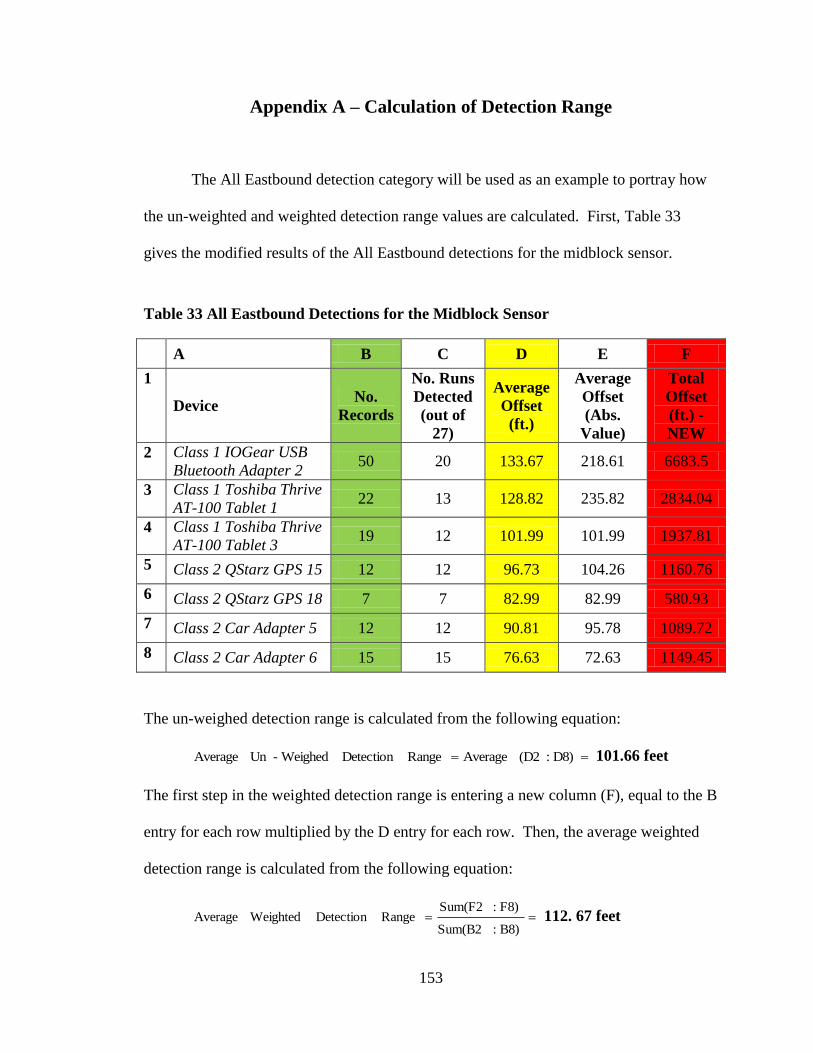
153
Appendix A – Calculation of Detection Range
The All Eastbound detection category will be used as an example to portray how
the un-weighted and weighted detection range values are calculated. First, Table 33
gives the modified results of the All Eastbound detections for the midblock sensor.
Table 33 All Eastbound Detections for the Midblock Sensor
A B C D E F
1
Device No.
Records
No. Runs
Detected
(out of
27)
Average
Offset
(ft.)
Average
Offset
(Abs.
Value)
Total
Offset
(ft.) -
NEW
2 Class 1 IOGear USB
Bluetooth Adapter 2 50 20 133.67 218.61 6683.5
3 Class 1 Toshiba Thrive
AT-100 Tablet 1 22 13 128.82 235.82 2834.04
4 Class 1 Toshiba Thrive
AT-100 Tablet 3 19 12 101.99 101.99 1937.81
5 Class 2 QStarz GPS 15 12 12 96.73 104.26 1160.76
6 Class 2 QStarz GPS 18 7 7 82.99 82.99 580.93
7 Class 2 Car Adapter 5 12 12 90.81 95.78 1089.72
8 Class 2 Car Adapter 6 15 15 76.63 72.63 1149.45
The un-weighed detection range is calculated from the following equation:
D8):(D2 Average RangeDetection Weighed- UnAverage 101.66 feet
The first step in the weighted detection range is entering a new column (F), equal to the B
entry for each row multiplied by the D entry for each row. Then, the average weighted
detection range is calculated from the following equation:
B8):Sum(B2
F8):Sum(F2 RangeDetection WeightedAverage 112. 67 feet
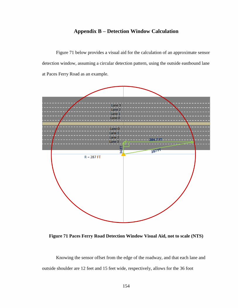
154
Appendix B – Detection Window Calculation
Figure 71 below provides a visual aid for the calculation of an approximate sensor
detection window, assuming a circular detection pattern, using the outside eastbound lane
at Paces Ferry Road as an example.
Figure 71 Paces Ferry Road Detection Window Visual Aid, not to scale (NTS)
Knowing the sensor offset from the edge of the roadway, and that each lane and
outside shoulder are 12 feet and 15 feet wide, respectively, allows for the 36 foot

155
measurement from the sensor to the middle of the inside lane. Then, the Pythagoras
Theorem allows for the calculation of the horizontal piece of the triangle. Doubling this
value gives the approximate distance that the lane spends in the sensor detection window.
This assumes that the antennae range is symmetric in either direction given that the
antenna points directly at the road. Then, giving different travel speeds, the time a lane is
spending in the detection window for different levels of congestion may be calculated.
By summing these times for all the eastbound lanes and all the westbound lanes
separately, one can calculate the proportion of time each direction spends in the sensor’s
detection window.

156
Appendix C – Chi Squared Test for MAC Address Detection Frequency
The first step in the Chi Squared test is to define the null and alternative
hypotheses.
Ho = MAC addresses detected ≤6 times and MAC addresses detected >6 times
DO NOT produce different travel times
Ho = MAC addresses detected ≤6 times and MAC addresses detected >6 times
DO produce different travel times
After defining the null hypothesis, the travel time must be broken up into bins so
that each bin has at least five records to qualify the Chi Squared test. Figure 72 shows
the travel time distribution for the two groups identified in the null hypothesis.
Figure 72 Travel Time Distribution Comparing Effect of MAC Address Frequency
0
2
4
6
8
10
12
14
16
18
20
1 3 5 7 9 11 13 15 17 19 21 23 25 27 29 31 33 35
Fre
qu
en
cy
Travel Time (Min.)
MACs with Less than orEqual to 6 Detections
MACs with Greater than 6Detections

157
Table 34 below shows the travel time broken into appropriate bins, as well as the
observed values for ≤6 and >6 MAC address repetitions for each bin. The table also
shows the sum values for each row and column, which combine to produce the expected
values via the equation shown below.
Table 34 Observed Values for MAC Frequency Categories
Travel Time Bins MACs with ≤6
Repetitions
MACs with >6
Repetitions Sum
0-16 64 5 69
17-18 27 9 36
19-20 34 5 39
21-22 30 7 37
23-35 33 10 43
Sum 188 36 N=224
N Total
TotalColumn Total Row Value Expected
Table 35 shows the expected values for the same bin and MAC frequency
combinations.
Table 35 Expected Values for MAC Frequency Categories
Travel Time Bins MACs with ≤6
Repetitions
MACs with >6
Repetitions
0-16 57.91 11.09
17-18 30.21 5.79
19-20 32.73 6.27
21-22 31.05 5.95
23-35 36.09 6.91
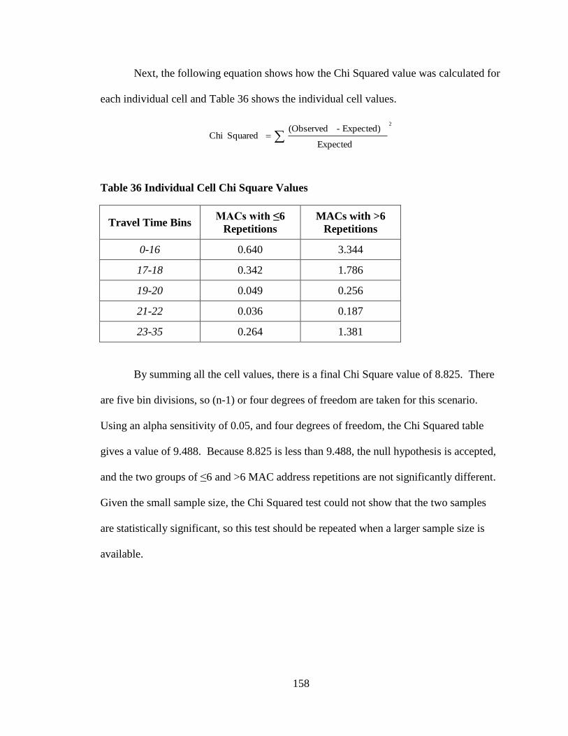
158
Next, the following equation shows how the Chi Squared value was calculated for
each individual cell and Table 36 shows the individual cell values.
2
Expected
Expected) - (Observed Squared Chi
Table 36 Individual Cell Chi Square Values
Travel Time Bins MACs with ≤6
Repetitions
MACs with >6
Repetitions
0-16 0.640 3.344
17-18 0.342 1.786
19-20 0.049 0.256
21-22 0.036 0.187
23-35 0.264 1.381
By summing all the cell values, there is a final Chi Square value of 8.825. There
are five bin divisions, so (n-1) or four degrees of freedom are taken for this scenario.
Using an alpha sensitivity of 0.05, and four degrees of freedom, the Chi Squared table
gives a value of 9.488. Because 8.825 is less than 9.488, the null hypothesis is accepted,
and the two groups of ≤6 and >6 MAC address repetitions are not significantly different.
Given the small sample size, the Chi Squared test could not show that the two samples
are statistically significant, so this test should be repeated when a larger sample size is
available.
159
References
1. “Bluetooth Tutorial – Baseband” Palowireless Bluetooth Resource Center,
Accessed from http://palowireless.com/bluearticles/baseband.asp
2. Johnson Consulting (2004) “Bluetooth – An Overview: How Networks Are
Formed and Controlled,” Accessed from
http://www.swedetrack.com/images/bluet10.htm
3. G. Zaruba, et al., (2004) “Simplified Bluetooth Device Discovery – Analysis and
Simulation” The University of Texas at Arlington, Proceedings of the 37th
Hawaii
International Conference on System Sciences, Accessed from
http://crystal.uta.edu/~zaruba/Publications/C20.pdf
4. G. Kewney, (2004) “High Speed Bluetooth Comes a Step Closer: Enhanced Data
Rate Approved,” Access from http://www.newswireless.net/index.cfm/article/629
5. S. Quale, et al., (2010) “Arterial Performance Measures with Media Access Control
Readers; Portland, Oregon, Pilot Study” Transportation Research Board of the
National Academies, Washington, D.C. Transportation Research Record No. 2192,
pg. 185-193
6. Motorola (2008) “Bluetooth Radio Performance Technical Brief: Rugged
Bluetooth Scanners” Access from
7. M. Loy, et al., (2005) “ISM-Band and Short Range Device Regulatory Compliance
Overview” Texas Instruments, Application Report SWRA048, Accessed from
http://www.ti.com/lit/an/swra048/swra048.pdf
8. Semtech International AG (2006) “FCC Regulations for ISM Band Devices: 902-
928 MHz” AN1200.04, Wireless and Sensing Products, Accessed from
http://www.semtech.com/images/datasheet/fcc_part15_regulations_ag.pdf
9. University of Maryland (2008) “Bluetooth Traffic Monitoring Technology;
Concept of Operation and Deployment Guidelines” Center for Advanced
Transportation Technology
10. R. Woodings, et al., (2001) “Rapid Heterogeneous Connection Establishment:
Accelerating Bluetooth Inquiry Using IrDA” Department of Computer Science,
Bringham Young University, Accessed from
http://mcl.cs.byu.edu/downloads/IrDA_Assisted_BT_Discovery.pdf
11. “Bluetooth Tutorial – Bluetooth Glossary” Palowireless Bluetooth Resource
Center, Accessed from http://www.palowireless.com/infotooth/glossary.asp
160
12. L. Harte, (2010) “Introduction to Bluetooth: Technology, Market, Operation,
Profiles, and Services,” Second Edition, Athos Publishing, Fuquay-Varina, North
Carolina
13. “Bluetooth Radio Layer Tutorial” Palowireless Bluetooth Resource Center,
Accessed from http://www.palowireless.com/infotooth/tutorial/radio.asp
14. D. Chakraborty, et al., (2006) "Discovery and Delay Analysis of Bluetooth
Devices," 7th International Conference on Mobile Data Management, Accessed
from http://ieeexplore.ieee.org/stamp/stamp.jsp?tp=&arnumber=1630650
15. B. Peterson, et al., (2006) “Bluetooth Inquiry Time Characterization And
Selection”, IEEE Transactions On Mobile Computing, Vol. 5, No. 9. Accessed
from http://ieeexplore.ieee.org/stamp/stamp.jsp?tp=&arnumber=1661527
16. Federal Highway Administration FHWA (2004) “Intelligent Transportation
Systems in Work Zones: A Case Study: Work Zone Travel Time System”,
Accessed from http://ops.fhwa.dot.gov/wz/technologies/arizona/arizona.pdf
17. Ontario Ministry of Transportation (2011) “Saddle up with Bluetooth: MTO First
in Canada to use Bluetooth for Travel Time Monitoring” Ontario’s Transportation
Technology Transfer Digest, Summer 2011, Vol. 17, Issue 3, Access from
http://www.mto.gov.on.ca/english/transtek/roadtalk/rt17-3/index.shtml#a3
18. A. Voigt, (2011) “Collecting External Data Using Bluetooth Technology”, Texas
Transportation Institute, Houston, TRB 90th
Annual Meeting, Session 175,
PowerPoint Presentation
19. “Bluetooth Radio Communications” Stevens Water Monitoring Systems, Inc.,
Accessed from http://www.stevenswater.com/telemetry_com/bluetooth_info.aspx
20. (2012) “XRange2000” Mind Vision Consulting, BlueMagnet, Accessed from
http://www.bluemagnet.com/xrange2000.html
21. A. Haghani, et al., (2010) “Data Collection of Freeway Travel Time Ground Truth
with Bluetooth Sensors” Transportation Research Record: Journal of the
Transportation Research Board, No. 2160
22. (2011) “Bluetooth Versions”, SP Commerce LLC, Accessed from
http://bluetomorrow.com
23. J. Porter, D. Kim, and M. Magana (2011) “Wireless Data Collection Systems for
Real-Time Arterial Travel Time Estimates” RS 500-410, Oregon Department of
Transportation and Oregon Transportation Research and Education Center

161
24. S.M. Baker (2010) “Bluetooth Technology to be Standard in More Than 90 Percent
of Automobiles by 2016” Kirkland, WA, November 18th
, 2010, Accessed from
http://www.bluetooth.com/Pages/Press-Releases-Detail.aspx?ItemID=117
25. Governors Highway Safety Association (2012) “Cell Phone and Texting Laws”,
State Laws and Funding, Accessed from
http://www.ghsa.org/html/stateinfo/laws/cellphone_laws.html
26. C. Monsere, et al., (2006) “Validating Dynamic Message Sign Freeway Travel
Time Messages with Ground Truth Geospatial Data” Transportation Research
Record No. 1959
27. J.S. Wasson, et al., (2008) “Real-Time Travel Time Estimates Using Media Access
Control Matching” ITE Journal, June 2008.
28. L. Tudor, et al., (2003) “Deployment of Smart Work Zone Technology in
Arkansas” Transportation Research Record No. 1824, Accessed from
http://trb.metapress.com/content/e2655n7753500257/fulltext.pdf
29. R. Varon, (2010) “Sensors Use Bluetooth to Compute Travel Times on Ike”, ABC
7 News, Chicago, IL, Accessed from
http://abclocal.go.com/wls/story?section=resources/traffic&id=7473453
30. R.J. Haseman, et al., (2010) “Real-Time Measurement of Travel Time Delay in
Work Zones and Evaluation Metrics Using Bluetooth Probe Tracking”,
Transportation Research Record No. 2169
31. C.A. Quiroga and D. Bullock (1998) “Determination of Sample Sizes for Travel
Time Studies” ITE Journal, August 1998, Accessed from
http://www.ite.org/membersonly/itejournal/pdf/JHA98A92.pdf
32. Texas A&M Transportation Institute (2012) “TTI-Designed Information System
Helps Keep I-35 Travelers Informed”, September 28, 2012, Accessed from
http://tti.tamu.edu/2012/09/28/tti-designed-information-system-helps-keep-i-35-
travelers-informed/
33. H.T. Zwahlen and A. Russ (2002) “Evaluation of the Accuracy of a Real-Time
Travel Time Prediction System in a Freeway Construction Work Zone”
Transportation Research Record No. 1803, Paper No. 02-2371
34. Federal Highway Administration (2008) “Comparative Analysis Report: The
Benefits of Using Intelligent Transportation Systems in Work Zones”, U.S.

162
Department of Transportation, Report Number FHWA-HOP-09-002. Accessed
from http://ops.fhwa.dot.gov/wz/its/wz_comp_analysis/comp_anl_rpt_08.pdf
35. Vehicle Detector Clearinghouse (2007) “A Summary of Vehicle Detection and
Surveillance Technologies Used In Intelligent Transportation Systems” Federal
Highway Administration, Accessed from
http://www.fhwa.dot.gov/policyinformation/pubs/vdstits2007/vdstits2007.pdf
36. T. Notbohm, et al., (2001) “Smart Work Zone Deployment Initiative Summer 2001
Travel Time Prediction System (TIPS)” Wisconsin Evaluation, Accessed from
http://www.eng.mu.edu/~drakopoa/web_documents/TIPS/Tipswisconsin.pdf
37. S. Du, et al., (2012) “Automatic License Plate Recognition (ALPR): A State of the
Art Review” IEEE Transactions on Circuits and Systems for Video Technology,
Accessed from http://ieeexplore.ieee.org/stamp/stamp.jsp?tp=&arnumber=6213519
38. Y. Malinovskiy, et al., (2009) “Field Experiments on Bluetooth-based Travel Time
Data Collection” University of Washington, Accessed from
http://staff.washington.edu/yegorm/Papers/2009_TRB_Bluetooth.pdf
39. J. Barcelo, et al., (2010) “Travel Time Forecasting and Dynamic Origin-
Destination Estimation for Freeways Based on Traffic Monitoring” Transportation
Research Record No. 2175, Accessed from
http://trb.metapress.com/content/17x1v88n6p8363p1/fulltext.pdf
40. S. Box (2011) “Arterial Roadway Traffic Data Collection Using Bluetooth
Technology” Master’s Thesis, Georgia Institute of Technology
41. DVDVideoSoft “Free Video to JPG Convertor” Accessed from
http://www.dvdvideosoft.com/products/dvd/Free-Video-to-JPG-Converter.htm
42. K. D’Ambrosio (2011) “Methodology for Collecting Vehicle Occupancy Data on
Multi-Lane Interstate Highways: A GA 400 Case Study” Master’s Thesis, Georgia
Institute of Technology