1  

A MILP model for the Teacher Assignment Problem

considering teachers’ preferences

Domenech B*, Lusa A

Department of Management (DOE); Institute of Industrial and Control Engineering (IOC)

Universitat Politècnica de Catalunya (UPC). Av. Diagonal 647 – floor 11, 08029, Barcelona (Spain).

Corresponding author (*): (+34) 934 016 579; bruno.domenech@upc.edu

Abstract

The Teacher Assignment Problem is part of the University Timetabling Problem and involves assigning

teachers to courses, taking their preferences into consideration. This is a complex problem, usually solved

by means of heuristic algorithms. In this paper a Mixed Integer Linear Programing model is developed to

balance teachers’ teaching load (first optimization criterion), while maximizing teachers’ preferences for

courses according to their category (second optimization criterion). The model is used to solve the

teachers-courses assignment in the Department of Management at the School of Industrial Engineering of

Barcelona, in the Universitat Politècnica de Catalunya. Results are discussed regarding the importance

given to the optimization criteria. Moreover, to test the model’s performance a computational experiment

is carried out using randomly generated instances based on real patterns. Results show that the model is

proven to be suitable for many situations (number of teachers/courses and weight of the criteria), being

useful for departments with similar requests.

Keywords: Timetabling; Linear programming; Teacher assignment problem; MILP model.

1. Introduction

The Timetabling Problem involves organizing a set of elements (which can be persons,

objects, meetings, etc.) in time. It has been demonstrated that if all possible solutions

were to be examined even for a reasonable amount of elements, the calculation time

would be excessively high (NP-hard problem) [Avella & Vasil’Ev, 2005]. This

complexity has led to the development of several models and heuristics to solve a wide

range of problems for many applications [Gunawan & Ng, 2011]. Among others, the

educational domain, and particularly the University Timetabling Problem, has been

much studied. Carter & Laporte [1998] proposed an interesting classification for this

problem: (1) Course Timetabling, to schedule courses respecting syllabus as well as

2  

classroom and teachers’ availability; (2) Class-Teacher Timetabling, to plan class-

teacher meetings avoiding overlaps for a given teacher assignment to courses and

classrooms; (3) Student Scheduling, to plan the sections of courses respecting classroom

capacities once students have chosen courses; (4) Teacher Assignment, to assign

teachers to courses maximizing a preference function; and (5) Classroom Assignment,

to assign events to classrooms once the event timetable has been scheduled.

The University Timetabling Problem and its sub-problems have been studied in detail

during the last five decades. Due to computational limitations when increasing the

number of teachers and courses involved, many heuristics and metaheuristics (such as

simulated annealing, genetic algorithms or tabu search) have been developed according

to the specific problem to be dealt with [Carter & Laporte, 1998]. However, thanks to

recent advances in computer software and hardware, Mixed Integer Linear

Programming (MILP) models have been used to solve the University Timetabling

Problem, obtaining optimal or near-to-optimal solutions [Johnson et al., 2000; Avella &

Vasil’Ev, 2005]. These models have usually been solved using efficient solution

procedures, such as Lagrangean relaxations [Daskalaki et al., 2004].

For example, over the last decade, Dimopoulou & Miliotis [2001] proposed an integer

programming model to build a combined courses-examinations timetable for a Greek

university, considering classroom availability and students’ flexibility in their choice of

courses. A constraint programming approach was developed by Valouxis and Housos

[2003] assuming that teachers move from one classroom to another, while students

always remain in the same classroom. Idle hours between the daily teaching

responsibilities are minimized and teachers’ requests for early or late shift assignments

are satisfied. The model was applied to typical Greek high schools. Daskalaki et al.

[2004] solved the university timetabling problem for an Engineering Department with a

large number of courses and teachers at a Greek University. The authors developed an

integer programming model that respects many operational rules from most universities

while satisfying expressed preferences for teaching periods, days of the week and

classrooms for courses. Later, Daskalaki & Birbas [2005] proposed an alternative

solution approach for the previous model. Al-Yakoob & Sherali [2007] faced the

problem of a university in Kuwait in assigning classes to time slots observing gender

policies, as well as dealing with parking and traffic congestion.

3  

Following the classification proposed by Carter & Laporte [1998], this paper focusses

on the Teacher Assignment Problem (4), which is one of the least studied sub-problems.

In most works dealing with this problem, the assignment is solved before scheduling

courses in time [Gunawan et al., 2008]. In contrast, very few papers focus on the

opposite option: to assign teachers to courses once the courses have been scheduled. In

this case, the main difficulty is to include teachers’ preferences for courses, since this

choice has to be adapted to the course timetables. To solve this problem, the approaches

that have primarily been used are meta-heuristics, multicriteria decision processes or

case-based approaches, among others [Petrovic & Burke, 2004]. One of the first MILP

models developed to solve the Teacher Assignment problem was proposed by Tillet

[1975], to maximize a preference function, combining both the teachers’ and the

department manager’s preferences. Selim [1982] designed a complex algorithm to

assign teachers to courses considering teachers’ availability and department requests for

courses (such as courses that may not be taught at the same time). Dinkel et al. [1989]

developed a decision support system to assist in maximizing teachers’ satisfaction and

improving classroom utilization in the teachers-courses assignment. Fahrion &

Dollansky [1992] designed an algorithm to assign faculty members to courses, which

included a priori fixed assignment options, such as desired classrooms according to size

or the availability of auxiliary support. Hultberg & Cardoso [1997] proposed a MILP

model, basing the formulation as a fixed charge transportation problem, to assign

teachers to courses while minimizing the average number of distinct subjects taught by

each teacher. Wang [2002] presented an approach based on genetic algorithms,

distinguishing between hard constraints (that necessarily have to be met) and soft

constraints (that have to be satisfied as much as possible). Another approach, used

recently by Gunawan et al. [2008; 2011], combines simulated annealing and tabu search

metaheuristics, allowing each course to be taught by more than one teacher and limiting

the academic load on each teacher. This work has recently been extended in Gunawan et

al. [2012], where a Lagrangean relaxation is used to solve the mathematical models.

As a research extension, Gunawan et al. [2012] proposed developing models that allow

the requirements of more universities to be considered. In this context, this work aims to

solve the Teacher Assignment Problem for the Department of Management (DOE) at

the School of Industrial Engineering of Barcelona (ETSEIB) in the Universitat

Politècnica de Catalunya (UPC), Spain. The paper provides four main contributions:

4  

1. The University Timetabling Problem is solved, including two novel considerations

not studied together in literature, but necessary for the case study: balancing

teachers’ load (optimization criterion 1) and maximizing teachers’ preferences for

courses, considering their category (optimization criterion 2).

2. A MILP model is developed to solve the problem. As input data, the load, schedule

and other specific characteristics of teachers and courses are considered. As a result,

the most appropriate teacher-course assignment is obtained for the optimization

criteria.

3. The objective function of the MILP model is developed using weighting parameters

to assign more or less significance to the optimization criteria. The model is solved

by the case study, discussing results according to such parameters. The results prove

that the model allows for a wide range of situations to be modelled, depending on

the importance ascribed to the balance between teachers’ load and the satisfaction of

teachers’ preferences.

4. One of the major limitations identified in literature is that the proposed models

cannot be solved for big departments, the use of alternative solving procedures, such

as relaxations, heuristics or metaheuristics being necessary. Therefore, the

performance of the developed MILP model is tested, through a computational

experiment, for instances of up to 50 teachers and 200 courses. Results show that

the model can obtain acceptable solutions for up to 40 teachers in a maximum

calculation time of one hour; a short time considering the kind of problem to be

solved. The model can then be useful for departments with similar requests.

The rest of the paper is organized as follows. In Section 2 the target problem is defined

in detail, leading to the development of the MILP model in Section 3. The case study of

the DOE-ETSEIB-UPC is solved in Section 4, discussing results according to the

weighting parameters of the objective function. In Section 5 a computational experiment

is carried out to test the model’s performance. Finally, the main conclusions are

summarized in Section 6.

5  

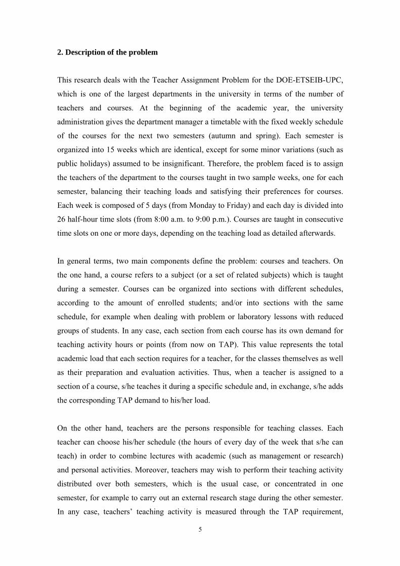
2. Description of the problem

This research deals with the Teacher Assignment Problem for the DOE-ETSEIB-UPC,

which is one of the largest departments in the university in terms of the number of

teachers and courses. At the beginning of the academic year, the university

administration gives the department manager a timetable with the fixed weekly schedule

of the courses for the next two semesters (autumn and spring). Each semester is

organized into 15 weeks which are identical, except for some minor variations (such as

public holidays) assumed to be insignificant. Therefore, the problem faced is to assign

the teachers of the department to the courses taught in two sample weeks, one for each

semester, balancing their teaching loads and satisfying their preferences for courses.

Each week is composed of 5 days (from Monday to Friday) and each day is divided into

26 half-hour time slots (from 8:00 a.m. to 9:00 p.m.). Courses are taught in consecutive

time slots on one or more days, depending on the teaching load as detailed afterwards.

In general terms, two main components define the problem: courses and teachers. On

the one hand, a course refers to a subject (or a set of related subjects) which is taught

during a semester. Courses can be organized into sections with different schedules,

according to the amount of enrolled students; and/or into sections with the same

schedule, for example when dealing with problem or laboratory lessons with reduced

groups of students. In any case, each section from each course has its own demand for

teaching activity hours or points (from now on TAP). This value represents the total

academic load that each section requires for a teacher, for the classes themselves as well

as their preparation and evaluation activities. Thus, when a teacher is assigned to a

section of a course, s/he teaches it during a specific schedule and, in exchange, s/he adds

the corresponding TAP demand to his/her load.

On the other hand, teachers are the persons responsible for teaching classes. Each

teacher can choose his/her schedule (the hours of every day of the week that s/he can

teach) in order to combine lectures with academic (such as management or research)

and personal activities. Moreover, teachers may wish to perform their teaching activity

distributed over both semesters, which is the usual case, or concentrated in one

semester, for example to carry out an external research stage during the other semester.

In any case, teachers’ teaching activity is measured through the TAP requirement,

6  

which depends on the category (as detailed next) and some other management activities

performed. There are six categories, representing teachers’ research, academic and

management expertise: Full Professor, Reader, Lecturer, Contributor, Assistant and Part

Time Lecturer. Apart from different TAP requirements, the main difference between

them for the purpose of this paper is that the first five categories are full time teachers

and represent the principal university staff. However, some unexpected events, such as a

higher than expected amount of students enrolled, or some particularities in the courses,

needing the expertise of somebody working in the industry, may require some Part

Time Lecturers. These teachers are employed by the university for a short period and a

specific activity. Therefore, the TAP requirement specified in their agreement must be

satisfied to ± 5%. In exchange, full time teachers can be more under or overloaded

(although respecting some reasonable limits) since their load can be easily balanced

from one year to another.

So far, the mandatory requirements of the problem have been presented. Additionally,

some other considerations are included to better represent real assignment requirements.

These considerations have been identified by collaborating with the manager of the

DOE-ETSEIB-UPC, who is the person in charge of the teachers-courses assignment:

1. To balance teachers’ load. Courses’ TAP demands and teachers’ TAP requirements

do not necessarily coincide. Thus, when dealing with the teachers-courses

assignment, some teachers can be under or overloaded. Varying the assignment, this

load can be concentrated in a reduced group of teachers or can be shared among all

of them. In the second case, teachers will globally be equally harmed or favored.

Hence, the equilibrium for the load among teachers must be achieved.

2. To satisfy teachers’ preferences for courses according to their category. As stated

before, there are six categories of teachers. The higher the category, the higher the

teacher’s teaching, research and management expertise, and so the priority when

meeting his/her preferences for courses and sections is also higher. Therefore,

satisfaction of teachers’ preferences for courses must be maximized, assuming a

certain index representing the category. In this way, the academic quality of the

department is expected to improve, since teachers will, generally, teach the courses

they desire.

7  

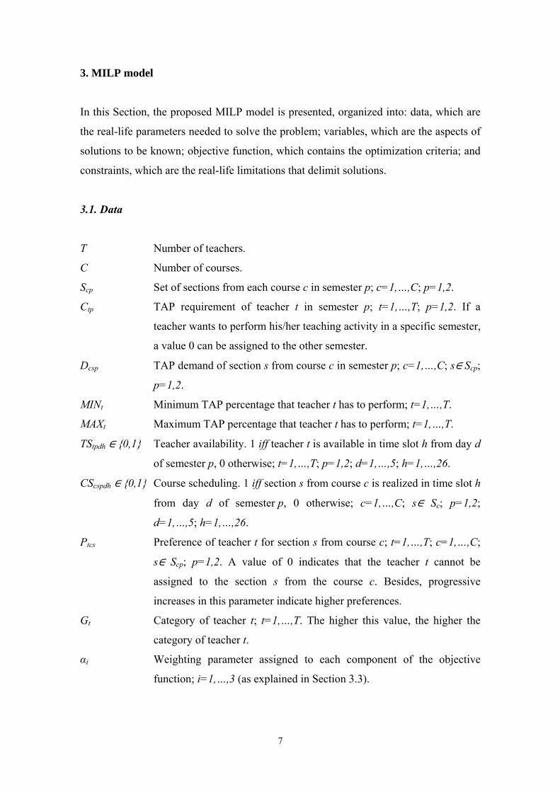
3. MILP model

In this Section, the proposed MILP model is presented, organized into: data, which are

the real-life parameters needed to solve the problem; variables, which are the aspects of

solutions to be known; objective function, which contains the optimization criteria; and

constraints, which are the real-life limitations that delimit solutions.

3.1. Data

T Number of teachers.

C Number of courses.

Scp Set of sections from each course c in semester p; c=1,…,C; p=1,2.

Ctp TAP requirement of teacher t in semester p; t=1,…,T; p=1,2. If a

teacher wants to perform his/her teaching activity in a specific semester,

a value 0 can be assigned to the other semester.

Dcsp TAP demand of section s from course c in semester p; c=1,…,C; s∈Scp;

p=1,2.

MINt Minimum TAP percentage that teacher t has to perform; t=1,…,T.

MAXt Maximum TAP percentage that teacher t has to perform; t=1,…,T.

TStpdh ∈ {0,1} Teacher availability. 1 iff teacher t is available in time slot h from day d

of semester p, 0 otherwise; t=1,…,T; p=1,2; d=1,…,5; h=1,…,26.

CScspdh ∈ {0,1} Course scheduling. 1 iff section s from course c is realized in time slot h

from day d of semester p, 0 otherwise; c=1,…,C; s∈ Sc; p=1,2;

d=1,…,5; h=1,…,26.

Ptcs Preference of teacher t for section s from course c; t=1,…,T; c=1,…,C;

s∈ Scp; p=1,2. A value of 0 indicates that the teacher t cannot be

assigned to the section s from the course c. Besides, progressive

increases in this parameter indicate higher preferences.

Gt Category of teacher t; t=1,…,T. The higher this value, the higher the

category of teacher t.

αi Weighting parameter assigned to each component of the objective

function; i=1,…,3 (as explained in Section 3.3).

8  

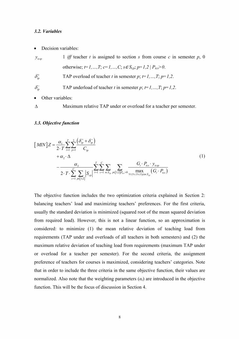
3.2. Variables

Decision variables:

tcspy 1 iff teacher t is assigned to section s from course c in semester p, 0

otherwise; t=1,…,T; c=1,…,C; s∈Scp; p=1,2 | Ptcs>0.

tp TAP overload of teacher t in semester p; t=1,…,T; p=1,2.

tp TAP underload of teacher t in semester p; t=1,…,T; p=1,2.

Other variables:

Maximum relative TAP under or overload for a teacher per semester.

3.3. Objective function

21

1 1

2

3

1 1 1;2 | 0; ; ; |

1 1;2

2

max2 cp tcscp

Ttp tp

t p tp

T Ct tcs tcsp

Ct c s S p P t tcs

t c s p s Scpc p

MIN ZT C

G P y

G PT S

(1)

The objective function includes the two optimization criteria explained in Section 2:

balancing teachers’ load and maximizing teachers’ preferences. For the first criteria,

usually the standard deviation is minimized (squared root of the mean squared deviation

from required load). However, this is not a linear function, so an approximation is

considered: to minimize (1) the mean relative deviation of teaching load from

requirements (TAP under and overloads of all teachers in both semesters) and (2) the

maximum relative deviation of teaching load from requirements (maximum TAP under

or overload for a teacher per semester). For the second criteria, the assignment

preference of teachers for courses is maximized, considering teachers’ categories. Note

that in order to include the three criteria in the same objective function, their values are

normalized. Also note that the weighting parameters (αi) are introduced in the objective

function. This will be the focus of discussion in Section 4.

9  

3.4. Constraints

1; | 0

1tcs

tcspt T P

y

1,..., ; ; 1,2cpc C s S p (2)

1 | 0cp tcs

C

tcsp csp tp tp tpc s S P

y D C

1,..., ; 1,2t T p (3)

2

1 1;2 | 0 1

·cp tcs

C

tcsp csp t tpc s S p P p

y D MIN C

1,...,t T (4)

2

1 1;2 | 0 1

·cp tcs

C

tcsp csp t tpc s S p P p

y D MAX C

1,...,t T (5)

tp tp

tpC

1,..., ; 1,2t T p (6)

1 | 0

1cp tcs

C

cspdh tcspc s S P

CS y

1,..., ; 1,2;

1,...,5; 1,...,26

t T p

d h

(7)

5 26 5 26

1 1 1 1tpdh cspdh tcsp cspdh

d h d h

TS CS y CS

1,..., ; 1,..., ; ;

1,2 | 0cp

tcs

t T c C s S

p P

(8)

; ; 0tp tp 1,..., ; 1,2t T p (9)

0,1tcspy 1, , ; 1, , ;

; 1,2 | 0cp tcs

t T c C

s S p P

(10)

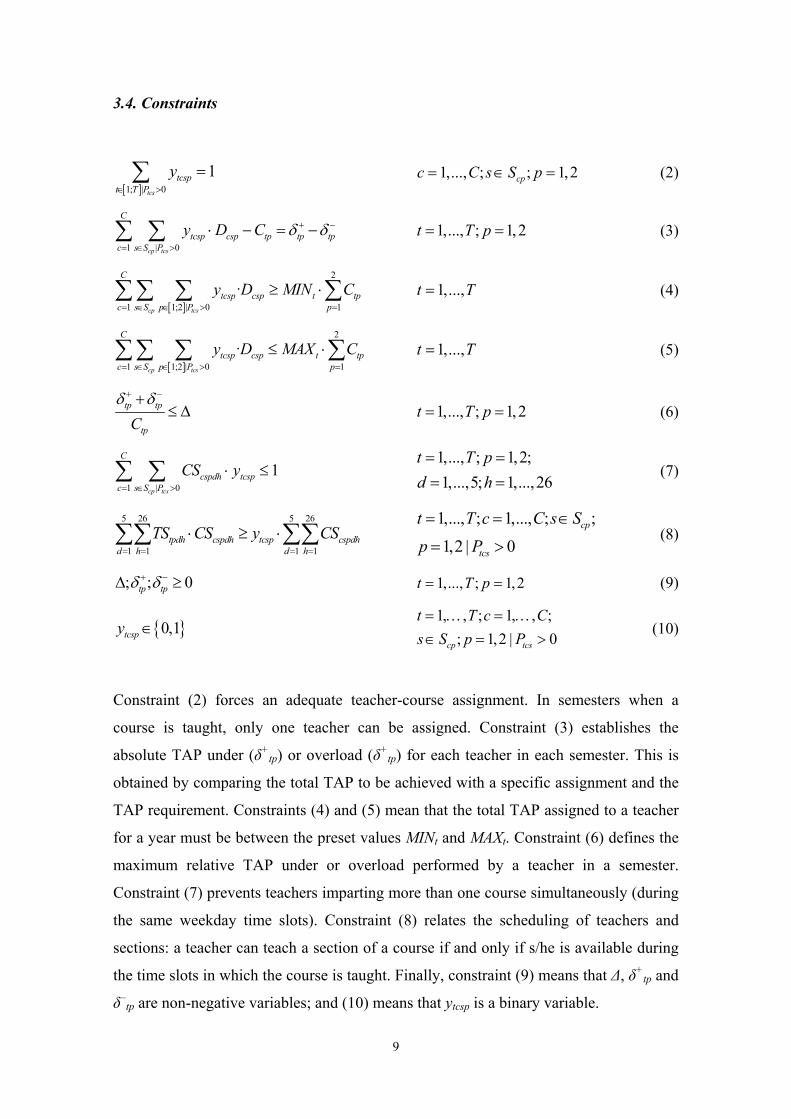
Constraint (2) forces an adequate teacher-course assignment. In semesters when a

course is taught, only one teacher can be assigned. Constraint (3) establishes the

absolute TAP under (δ+tp) or overload (δ+

tp) for each teacher in each semester. This is

obtained by comparing the total TAP to be achieved with a specific assignment and the

TAP requirement. Constraints (4) and (5) mean that the total TAP assigned to a teacher

for a year must be between the preset values MINt and MAXt. Constraint (6) defines the

maximum relative TAP under or overload performed by a teacher in a semester.

Constraint (7) prevents teachers imparting more than one course simultaneously (during

the same weekday time slots). Constraint (8) relates the scheduling of teachers and

sections: a teacher can teach a section of a course if and only if s/he is available during

the time slots in which the course is taught. Finally, constraint (9) means that Δ, δ+tp and

δ–tp are non-negative variables; and (10) means that ytcsp is a binary variable.

10  

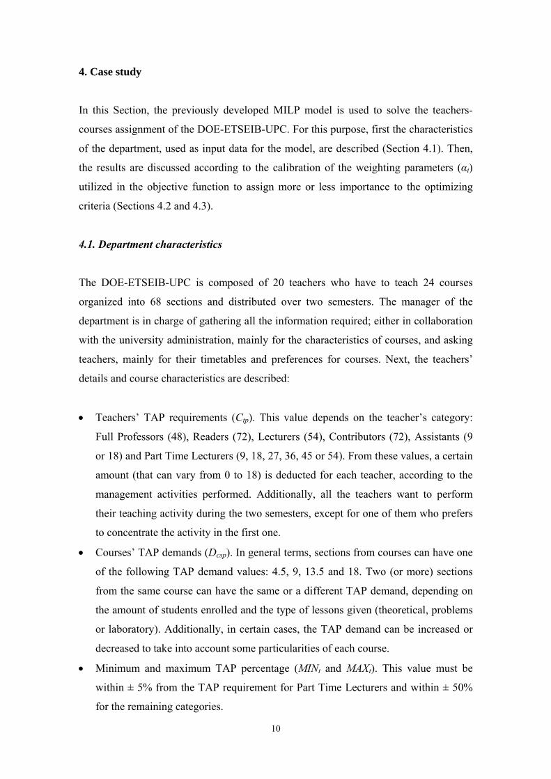
4. Case study

In this Section, the previously developed MILP model is used to solve the teachers-

courses assignment of the DOE-ETSEIB-UPC. For this purpose, first the characteristics

of the department, used as input data for the model, are described (Section 4.1). Then,

the results are discussed according to the calibration of the weighting parameters (αi)

utilized in the objective function to assign more or less importance to the optimizing

criteria (Sections 4.2 and 4.3).

4.1. Department characteristics

The DOE-ETSEIB-UPC is composed of 20 teachers who have to teach 24 courses

organized into 68 sections and distributed over two semesters. The manager of the

department is in charge of gathering all the information required; either in collaboration

with the university administration, mainly for the characteristics of courses, and asking

teachers, mainly for their timetables and preferences for courses. Next, the teachers’

details and course characteristics are described:

Teachers’ TAP requirements (Ctp). This value depends on the teacher’s category:

Full Professors (48), Readers (72), Lecturers (54), Contributors (72), Assistants (9

or 18) and Part Time Lecturers (9, 18, 27, 36, 45 or 54). From these values, a certain

amount (that can vary from 0 to 18) is deducted for each teacher, according to the

management activities performed. Additionally, all the teachers want to perform

their teaching activity during the two semesters, except for one of them who prefers

to concentrate the activity in the first one.

Courses’ TAP demands (Dcsp). In general terms, sections from courses can have one

of the following TAP demand values: 4.5, 9, 13.5 and 18. Two (or more) sections

from the same course can have the same or a different TAP demand, depending on

the amount of students enrolled and the type of lessons given (theoretical, problems

or laboratory). Additionally, in certain cases, the TAP demand can be increased or

decreased to take into account some particularities of each course.

Minimum and maximum TAP percentage (MINt and MAXt). This value must be

within ± 5% from the TAP requirement for Part Time Lecturers and within ± 50%

for the remaining categories.

11  

Teacher availability (TStpdh). In general terms, teachers are available at any moment

of the week, except for some occasional exceptions early in the morning or late in

the afternoon, mainly due to personal incompatibilities.

Course scheduling (CScspdh). The timetable of each course basically depends on the

TAP demand: for 4.5 TAP courses, 1 hour/week; for 9 TAP courses, 2 hours/week;

for 13.5 TAP courses, 3 hours/week; and for 18 TAP courses, 4 hours/week.

Preference (Ptcs). A 0 is assigned to teachers who cannot teach a course; a 1 refers to

teachers who could teach a course; and a 3 is for teachers who are particularly

interested in a course.

Category (Gt). A value is assigned to each category: Full Professors (0.286),

Readers (0.238), Lecturers (0.190), Contributors (0.143), Assistants (0.095) and Part

Time Lecturers (0.048). These values were determined by the DOE-ETSEIB-UPC

manager, after discussing with teachers of different categories of the department.

With this information, the model can be solved and it is expected that the teachers-

courses assignment that best balances teachers’ load and satisfies their preferences will

be obtained for the DOE-ETSEIB-UPC. However, depending on the weighting

parameters (αi) from the objective function, the solution might logically vary. In fact,

the calibration of the cost coefficients has been a widely discussed subject in literature

[Daskalaki et al., 2004]. Therefore, results are discussed according to such parameters in

the next two Sections: first α1 and α2 are calibrated, since they both refer to achieving a

balanced load among teachers; and then their combination is calibrated regarding α3

(teachers’ preferences).

4.2. First calibration

As stated previously, an adequate strategy for balancing teachers’ load consists in

minimizing the standard deviation of the TAP assignment. However, this would not be a

linear option, so an approximation is considered: to minimize the mean and the

maximum relative deviations of teaching loads from requirements. Both components are

respectively related to the weighting parameters α1 and α2. Therefore, the aim of the first

calibration is to determine the values of α1 and α2 that minimize the global standard

deviation. Thus, the calibration parameter λI is defined according to equation (11):

12  

2

1 1

11

2

Ttp tp

I It p tpT C

(11)

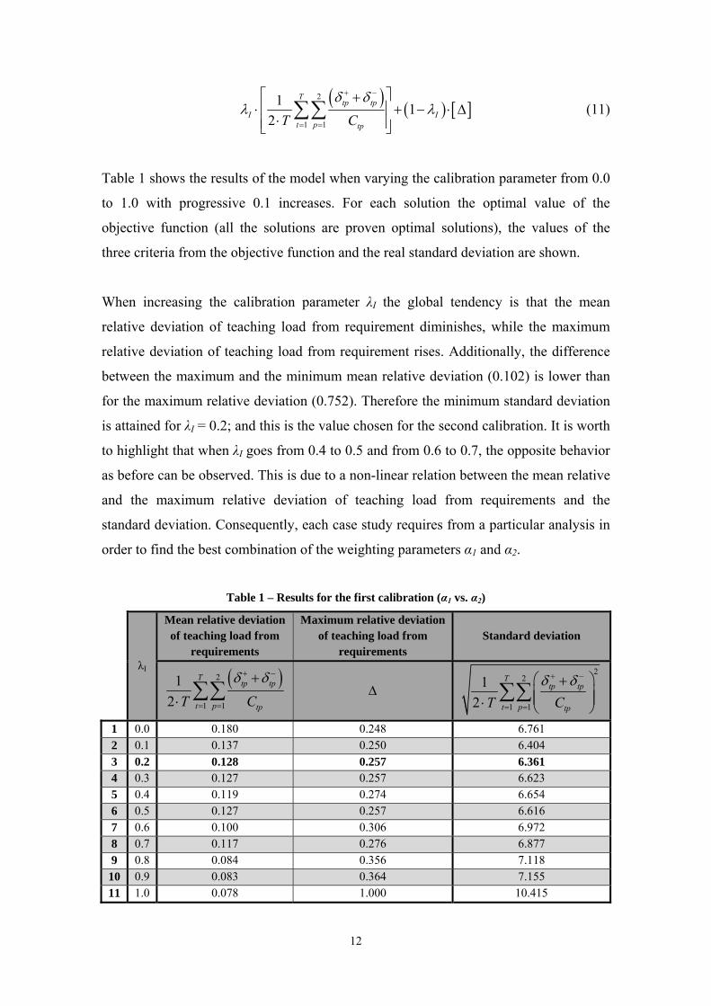
Table 1 shows the results of the model when varying the calibration parameter from 0.0

to 1.0 with progressive 0.1 increases. For each solution the optimal value of the

objective function (all the solutions are proven optimal solutions), the values of the

three criteria from the objective function and the real standard deviation are shown.

When increasing the calibration parameter λI the global tendency is that the mean

relative deviation of teaching load from requirement diminishes, while the maximum

relative deviation of teaching load from requirement rises. Additionally, the difference

between the maximum and the minimum mean relative deviation (0.102) is lower than

for the maximum relative deviation (0.752). Therefore the minimum standard deviation

is attained for λI = 0.2; and this is the value chosen for the second calibration. It is worth

to highlight that when λI goes from 0.4 to 0.5 and from 0.6 to 0.7, the opposite behavior

as before can be observed. This is due to a non-linear relation between the mean relative

and the maximum relative deviation of teaching load from requirements and the

standard deviation. Consequently, each case study requires from a particular analysis in

order to find the best combination of the weighting parameters α1 and α2.

Table 1 – Results for the first calibration (α1 vs. α2)

λI

Mean relative deviation of teaching load from

requirements

Maximum relative deviation of teaching load from

requirements Standard deviation

2

1 1

1

2

Ttp tp

t p tpT C

22

1 1

1

2

Ttp tp

t p tpT C

1 0.0 0.180 0.248 6.761 2 0.1 0.137 0.250 6.404 3 0.2 0.128 0.257 6.361 4 0.3 0.127 0.257 6.623 5 0.4 0.119 0.274 6.654 6 0.5 0.127 0.257 6.616 7 0.6 0.100 0.306 6.972 8 0.7 0.117 0.276 6.877 9 0.8 0.084 0.356 7.118

10 0.9 0.083 0.364 7.155 11 1.0 0.078 1.000 10.415

13  

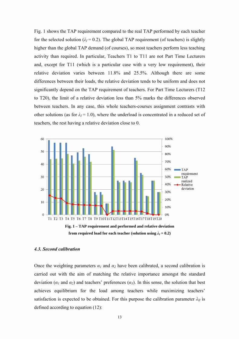
Fig. 1 shows the TAP requirement compared to the real TAP performed by each teacher

for the selected solution (λI = 0.2). The global TAP requirement (of teachers) is slightly

higher than the global TAP demand (of courses), so most teachers perform less teaching

activity than required. In particular, Teachers T1 to T11 are not Part Time Lecturers

and, except for T11 (which is a particular case with a very low requirement), their

relative deviation varies between 11.8% and 25.5%. Although there are some

differences between their loads, the relative deviation tends to be uniform and does not

significantly depend on the TAP requirement of teachers. For Part Time Lecturers (T12

to T20), the limit of a relative deviation less than 5% marks the differences observed

between teachers. In any case, this whole teachers-courses assignment contrasts with

other solutions (as for λI = 1.0), where the underload is concentrated in a reduced set of

teachers, the rest having a relative deviation close to 0.

Fig. 1 – TAP requirement and performed and relative deviation

from required load for each teacher (solution using λI = 0.2)

4.3. Second calibration

Once the weighting parameters α1 and α2 have been calibrated, a second calibration is

carried out with the aim of matching the relative importance amongst the standard

deviation (α1 and α2) and teachers’ preferences (α3). In this sense, the solution that best

achieves equilibrium for the load among teachers while maximizing teachers’

satisfaction is expected to be obtained. For this purpose the calibration parameter λII is

defined according to equation (12):

14  

2

1 1

1 1 1;2 | 0; ; ; |

1 1;2

11

2

11

max2 cp tcscp

Ttp tp

II I It p tp

T Ct tcs tcsp

II Ct c s S p P t tcs

t c s p s Scpc p

T C

G P y

G PT S

(12)

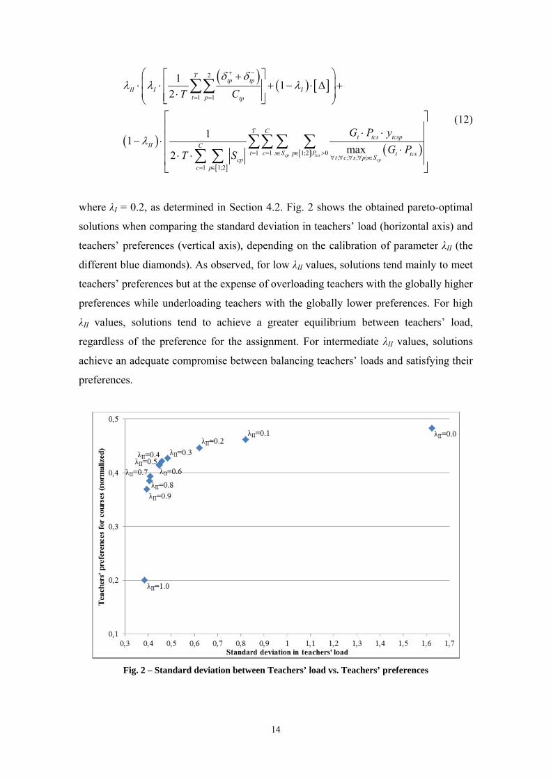
where λI = 0.2, as determined in Section 4.2. Fig. 2 shows the obtained pareto-optimal

solutions when comparing the standard deviation in teachers’ load (horizontal axis) and

teachers’ preferences (vertical axis), depending on the calibration of parameter λII (the

different blue diamonds). As observed, for low λII values, solutions tend mainly to meet

teachers’ preferences but at the expense of overloading teachers with the globally higher

preferences while underloading teachers with the globally lower preferences. For high

λII values, solutions tend to achieve a greater equilibrium between teachers’ load,

regardless of the preference for the assignment. For intermediate λII values, solutions

achieve an adequate compromise between balancing teachers’ loads and satisfying their

preferences.

Fig. 2 – Standard deviation between Teachers’ load vs. Teachers’ preferences

15  

All the options belong to the set of pareto-optimal solutions, i.e. efficient teachers-

courses assignments that minimize the standard deviation between teachers’ loads,

while maximizing teachers’ preferences. Therefore, each option can be chosen to be

implemented in the case study of the DOE-ETSEIB-UPC. The manager of the

department will choose the option according to what s/he considers to be more

appropriate. In this way the model can be adapted to different situations, not only

depending on teachers and courses, but also on the final decision-maker.

5. Computational experiment

As stated in Section 1, one of the major limitations of the use of MILP models for the

University Timetabling Problem, and particularly the Teaching Assignment Problem, is

the difficulty of finding a solution. For that reason several algorithms, heuristics and

metaheuristics, have usually been developed by researchers to solve their specific

versions of the problem. However, integer programming is gaining acceptance as a tool

to provide optimal or near-optimal solutions in progressively shorter running times

[Atamtürk & Savelsbergh, 2005]. Therefore, in this Section a computational experiment

is carried out in order to analyze the performance of the MILP model developed in

Section 3. For this purpose several instances are randomly generated, based on the

characteristics of the DOE-ETSEIB-UPC described in detail in Section 4. The data used

to generate the instances is described next:

Number of teachers (T): 10, 20, 30, 40, 50.

Number of courses (C): A reasonable number of courses is considered, depending

on the number of teachers. In particular the double, triple and quadruple ratio of

courses to teachers are studied.

Set of sections (Scp): Considering that this is a computational experiment to analyze

the performance of the model, and for the sake of clarity, a single section is

considered for each course.

Instances: 50.

16  

No more than 50 teachers (and consequently 200 courses) instances are generated since

these are sufficient to represent the kind of departments that could use the proposed

model. As a result of combining the 5 teacher scenarios, the 3 course scenarios and the

50 instances for each combination, 750 instances are solved. The rest of the data is also

generated randomly but ensuring that instances are solvable, since no particularized

study can be carried out for each instance. In this sense, a conservative philosophy is

respected, always based on the characteristics of the DOE-ETSEIB-UPC, giving a

realistic approach to each instance. The data used is listed next:

Teachers TAP requirement (Ctp).

o Full Professors (48 minus a random value between 0 and 18).

o Readers (72 minus a random value between 0 and 18).

o Lecturers (54 minus a random value between 0 and 18).

o Contributors (72 minus a random value between 0 and 18).

o Assistants (9 or 18 randomly).

o Part Time Lecturers (9 times a random value between 1 and 6).

Additionally, to better represent real departments, these values are proportionally

adapted, ensuring that the sum of TAP requirements is close to the sum of TAP

demands, with a margin of 5%.

Courses TAP demand (Dcsp). Four types of courses are considered (in similar

amounts) with the next TAP demands: 4.5, 9, 13.5 and 18.

Minimum and maximum TAP percentage (MINt and MAXt). Within ± 5% from the

TAP requirement for Part Time Lecturers and ± 50% for the other categories.

Teacher availability (TStpdh). All the teachers are available at any moment, to ensure

there are no incompatibilities due to a lack of teachers for a specific time slot.

Course scheduling (CScspdh). A different schedule type for each type of course:

o For 4.5 TAP courses, 2 consecutive time slots per day.

o For 9 TAP courses, 4 consecutive time slots per day.

o For 13.5 TAP courses, two groups of 3 consecutive time slots over different

days.

o For 18 TAP courses, two groups of 4 consecutive time slots over different days.

Preference (Ptcs). A value of 1 is established for each teacher-course pairing to

ensure the feasibility of solutions.

17  

Category (Gt). The category of each teacher is randomly chosen, approximately

respecting real proportions, and the values are maintained from the case study:

o 10% of Full Professors, Gt value 0.286.

o 30% of Readers, Gt value 0.238.

o 10% of Lecturers, Gt value 0.190.

o 10% of Contributors, Gt value 0.143.

o 15% of Assistants, Gt value 0.095.

o 25% of Part Time Lecturers, Gt value 0.048.

Weighting parameters of the objective function (α1, α2, α3): a random value is

defined for each one, but ensuring that the sum is 1. Note that the aim is not to study

the αi values, but to ensure that the model can be solved for any combination of αi.

To carry out the computational experiment, a maximum calculation time is set to 3600

seconds for each instance. The MILP model is solved using the IBM ILOG CPLEX

12.2 Optimizer, on a PC 3.16 GHz Intel Core 2 Duo E8500 with 3.46 GB of RAM.

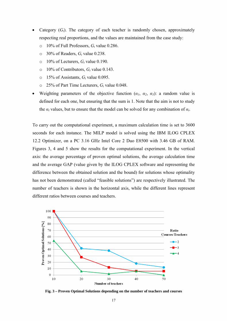
Figures 3, 4 and 5 show the results for the computational experiment. In the vertical

axis: the average percentage of proven optimal solutions, the average calculation time

and the average GAP (value given by the ILOG CPLEX software and representing the

difference between the obtained solution and the bound) for solutions whose optimality

has not been demonstrated (called “feasible solutions”) are respectively illustrated. The

number of teachers is shown in the horizontal axis, while the different lines represent

different ratios between courses and teachers.

Fig. 3 – Proven Optimal Solutions depending on the number of teachers and courses

18  

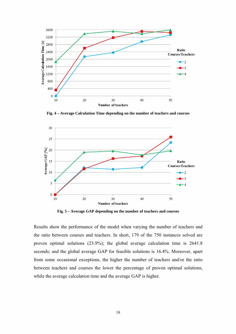
Fig. 4 – Average Calculation Time depending on the number of teachers and courses

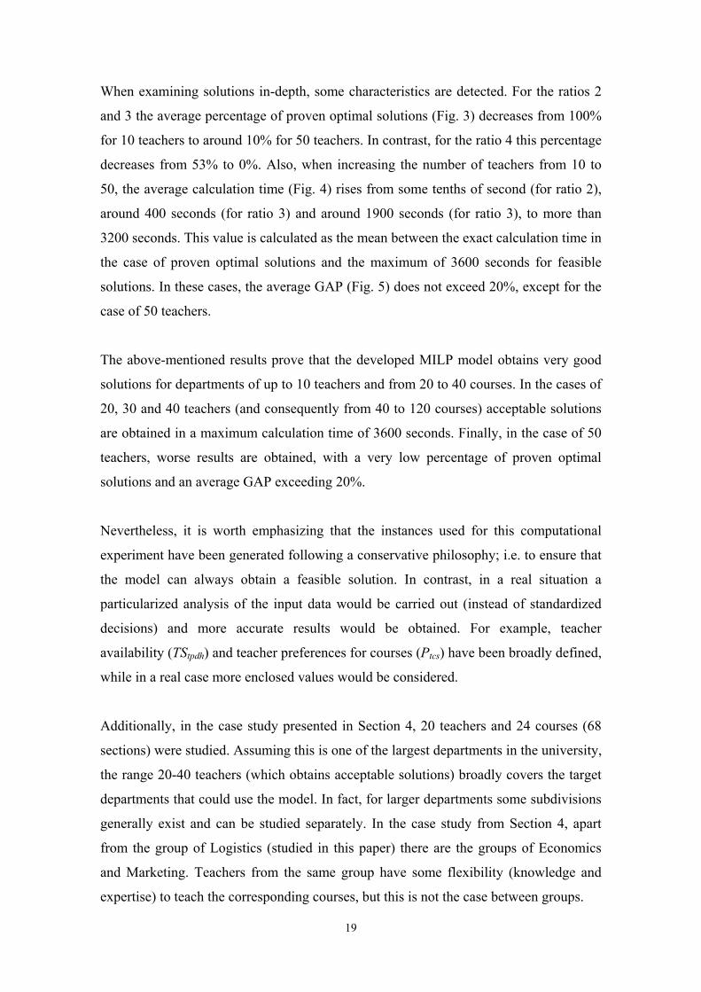
Fig. 5 – Average GAP depending on the number of teachers and courses

Results show the performance of the model when varying the number of teachers and

the ratio between courses and teachers. In short, 179 of the 750 instances solved are

proven optimal solutions (23.9%); the global average calculation time is 2641.8

seconds; and the global average GAP for feasible solutions is 16.4%. Moreover, apart

from some occasional exceptions, the higher the number of teachers and/or the ratio

between teachers and courses the lower the percentage of proven optimal solutions,

while the average calculation time and the average GAP is higher.

19  

When examining solutions in-depth, some characteristics are detected. For the ratios 2

and 3 the average percentage of proven optimal solutions (Fig. 3) decreases from 100%

for 10 teachers to around 10% for 50 teachers. In contrast, for the ratio 4 this percentage

decreases from 53% to 0%. Also, when increasing the number of teachers from 10 to

50, the average calculation time (Fig. 4) rises from some tenths of second (for ratio 2),

around 400 seconds (for ratio 3) and around 1900 seconds (for ratio 3), to more than

3200 seconds. This value is calculated as the mean between the exact calculation time in

the case of proven optimal solutions and the maximum of 3600 seconds for feasible

solutions. In these cases, the average GAP (Fig. 5) does not exceed 20%, except for the

case of 50 teachers.

The above-mentioned results prove that the developed MILP model obtains very good

solutions for departments of up to 10 teachers and from 20 to 40 courses. In the cases of

20, 30 and 40 teachers (and consequently from 40 to 120 courses) acceptable solutions

are obtained in a maximum calculation time of 3600 seconds. Finally, in the case of 50

teachers, worse results are obtained, with a very low percentage of proven optimal

solutions and an average GAP exceeding 20%.

Nevertheless, it is worth emphasizing that the instances used for this computational

experiment have been generated following a conservative philosophy; i.e. to ensure that

the model can always obtain a feasible solution. In contrast, in a real situation a

particularized analysis of the input data would be carried out (instead of standardized

decisions) and more accurate results would be obtained. For example, teacher

availability (TStpdh) and teacher preferences for courses (Ptcs) have been broadly defined,

while in a real case more enclosed values would be considered.

Additionally, in the case study presented in Section 4, 20 teachers and 24 courses (68

sections) were studied. Assuming this is one of the largest departments in the university,

the range 20-40 teachers (which obtains acceptable solutions) broadly covers the target

departments that could use the model. In fact, for larger departments some subdivisions

generally exist and can be studied separately. In the case study from Section 4, apart

from the group of Logistics (studied in this paper) there are the groups of Economics

and Marketing. Teachers from the same group have some flexibility (knowledge and

expertise) to teach the corresponding courses, but this is not the case between groups.

20  

In any case, the developed MILP model aims to replace the traditional manual process

of teacher assignment, which is a complex task usually carried out by the manager of

the department over several days in a kind of trial-and-error way and which requires a

deep knowledge of the problem. Therefore, the maximum calculation time for a

particular case study could be considerably extended and, together with a particularized

analysis of the input data, better solutions would surely be obtained.

6. Conclusions

This paper deals with the Teacher Assignment Problem, which involves assigning a set

of teachers to a set of courses with predefined schedules. For this purpose a MILP

model is developed that allows the balancing of the teachers’ load and the maximizing

of their preferences for courses, while considering the limitations of the problem itself:

teachers’ TAP requirements, category and schedule as well as courses’ TAP demands

and timetables. Moreover, some weighting parameters allow the importance of the

optimization criteria to be adjusted in order to adapt the results to different situations.

To validate the model two computational experiments are carried out. First, the

particular case of the DOE-ETSEIB-UPC is solved. For this purpose a two-step analysis

is performed. On the one hand, the balance between teachers’ load is studied, calibrating

the mean and the maximum relative deviations of teaching loads from requirements that

minimize the standard deviation. On the other hand, the balance between teachers’ load

and the maximization of teachers’ preferences are calibrated. In any case, results are

discussed according to the weighting parameters, proving that the model can be shaped

to the specific problem, thus being useful for other departments with similar requests.

Secondly, 750 instances based on real patterns are randomly generated but modifying

the number of teachers and courses. Results show that the model can be solved for

situations of up to 40 teachers, obtaining acceptable solutions in a reduced calculation

time.

21  

Acknowledgements

This paper was supported by the Spanish Ministry of Science and Innovation (project DPI 2010-15614).

The authors are very grateful for all the support given by the teachers and administrative staff of the

Department of Management at the School of Industrial Engineering of Barcelona in the Universitat

Politècnica de Catalunya. The authors would also like to thank the anonymous reviewers for their

valuable comments and suggestions on improving the paper.

References

1. Al-Yakoob, S. M., & Sherali, H. D. (2007). A mixed-integer programming approach to a class

timetabling problem: A case study with gender policies and traffic considerations. European Journal

of Operational Research, 180, 1028–1044.

2. Atamtürk, A., & Savelsbergh, M.W.P. (2005). Integer-programming software systems. Annals of

Operations Research, 140, 67–124.

3. Avella, P., & Vasil’ev, I. (2005). A computational study of a cutting plane algorithm for university

course timetabling. Journal of Scheduling, 8, 497–514.

4. Carter, M. W., & Laporte, G. (1998). Recent developments in practical course timetabling. In E. K.,

Burke, & P., Ross (Eds.), Selected papers from the 2nd International Conference on the Practice and

Theory of Automated Timetabling (pp. 3–19). Lecture Notes in Computer Science, Springer.

5. Daskalaki, S., Birbas, T., & Housos, E. (2004). An integer programming formulation for a case study

in university timetabling. European Journal of Operational Research, 153, 117–135.

6. Daskalaki, S., & Birbas, T. (2005). Efficient solutions for a university timetabling problem through

integer programming. European Journal of Operational Research, 160, 106–120.

7. Dimopoulou, M., & Miliotis, P. (2001). Implementation of a university course and examination

timetabling system. European Journal of Operational Research, 130, 202–213.

8. Dinkel, J. J., Mote, J., & Venkataramanan, M. A. (1989). An efficient decision support system for

academic course scheduling. Operations Research, 37, 853–864.

9. Fahrion, R., & Dollansky, G. (1992). Construction of university faculty timetables using logic

programming technique. Discrete Applied Mathematics, 35, 221–236.

10. Gunawan, A., Ng, K. M., & Ong, H. L. (2008). A genetic algorithm for the teacher assignment

problem for a university in Indonesia. International Journal of Information and Management

Sciences, 19, 1–16.

11. Gunawan, A., & Ng, K. M. (2011). Solving the teacher assignment problem by two metaheuristics.

International Journal of Information and Management Sciences, 22, 73–86.

12. Gunawan, A., Ng, K. M., & Poh, K. L. (2012). A hybridized Lagrangean relaxation and simulated

annealing method for the course timetabling problem. Computers & Operations Research, 39,

3074–3088.

22  

13. Hultberg, T. H., & Cardoso, D. M. (1997). The teacher assignment problem: A special case of the

fixed charge transportation problem. European Journal of Operational Research, 101, 463–473.

14. Johnson, E. L., Nemhauser, G. L., & Savelsbergh, M. W. P. (2000). Progress in linear programming

based branch-and-bound algorithms: An exposition. INFORMS Journal on Computing, 12.

15. Petrovic, S., & Burke, E. K. (2004). University Timetabling. In J. Leung (Ed.), Handbook of

scheduling: Algorithms, models, and performance analysis (chapter 45). CRC Press.

16. Selim, S. M. (1982). An algorithm for constructing a university faculty timetable. Computers &

Education, 6, 323–334.

17. Tillet, P. I. (1975). An operations research approach to the assignment of teachers to courses. Socio-

Economic Planning Sciences, 9, 101–104.

18. Valouxi,s C., Housos, E. (2003). Constraint programming approach for school timetabling.

Computers & Operations Research, 30, 1555–1572.

19. Wang, Y. Z. (2002). An application of genetic algorithm methods for teacher assignment problems.

Expert Systems with Applications, 22, 295–302.