a modified algorithm of steepest descent method for solving unconstrained … · 2016-01-29 · a...

88 Journal of Marine Science and Technology, Vol. 23, No. 1, pp. 88-97 (2015 ) DOI: 10.6119/JMST-014-0221-1

A MODIFIED ALGORITHM OF STEEPEST DESCENT METHOD FOR SOLVING

UNCONSTRAINED NONLINEAR OPTIMIZATION PROBLEMS

Chein-Shan Liu1, Jiang-Ren Chang2, and Yung-Wei Chen3

Key words: invariant manifold, generalized Rosenbrock function, modified steepest descent method (MSDM).

ABSTRACT

The steepest descent method (SDM), which can be traced back to Cauchy (1847), is the simplest gradient method for unconstrained optimization problem. The SDM is effective for well-posed and low-dimensional nonlinear optimization problems without constraints; however, for a large-dimensional system, it converges very slowly. Therefore, a modified steepest decent method (MSDM) is developed to deal with these problems. Under the MSDM framework, the original global minimization problem is transformed into a quadratic-form minimization based on the SDM and the current iterative point. Our starting point is a manifold defined in terms of the quadratic function and a fictitious time variable. Thereafter, we can derive an iterative algorithm by including a parameter in the final stage. Through a Hopf bifurcation, this parameter indeed plays a major role to switch the situation of slow con-vergence to a new situation that the new algorithm converges faster. Several numerical examples are examined and com-pared with exact solutions. It is found that the new algorithm of the MSDM has better computational efficiency and accu-racy, even for a large-dimensional non-convex minimization problem of the generalized Rosenbrock function.

I. INTRODUCTION

In this paper, we consider the following nonlinear optimi-

zation problem without constraints:

min ( ) 0f x , (1)

where f : Rn R is a C2 differentiable function. For solving (1), there are many approaches of iterative

types. If xk is the current iterative point, then we denote f(xk) by fk , f(xk) by gk and 2 f(xk) by Ak. The second order Taylor expansion of function f(x) at the point xk is

TT 1( )

2k k kf f x g x x A x , (2)

where x = x - xk. The superscript T signifies the transpose. Letting x = xk gk and inserting it into (2), we can obtain

2

T T( )2k k k k k k k kf f x g g g g A g . (3)

Taking a minimization with respect to , we can solve

2

T

k

k k k

g

g A g. (4)

Then the well-known steepest descent method (SDM) for solving (1) is obtained: (i) Give an initial x0, and then g0 = f(x0). (ii) For k = 0, 1, 2, ... we repeat the following calculations.

If k g , then stop; otherwise, let k = k + 1 and find the

next xk+1 by

2

1 T.k

k k kk k k

g

x x gg A g

(5)

Go to step (ii). Several modifications to the SDM have been addressed.

Paper submitted 08/15/13; revised 01/21/14; accepted 02/21/14. Author for correspondence: Yung-Wei Chen (e-mail: [email protected]). 1 Department of Civil Engineering, National Taiwan University, Taipei, Tai-wan, R.O.C.

2 Department of Systems Engineering and Naval Architecture, National Tai-wan Ocean University, Keelung, Taiwan, R.O.C.

3 Department of Marine Engineering, National Taiwan Ocean University, Keelung, Taiwan, R.O.C.

C.-S. Liu et al.: A Modified Steepest Decent Method (MSDM) 89

These modifications have led to a new interest in the SDM that the gradient vector itself is not a bad choice but rather that the original step-length leads to the slow convergence behavior. Barzilai and Browein (1988) were the first to present a new choice of step-length through two-point step-size. Although their method did not guarantee descent of the minimum func-tional values, it could produce a substantial improvement of the convergence speed for a two dimensional quadratic func-tion. According to their method, many researchers have pro-posed some choices of the step-length for the gradient method, for example, Raydan (1993; 1997); Friedlander et al. (1999); Dai and Liao (2002); Dai et al. (2002); Raydan and Svaiter (2002); Dai and Yuan (2003); Fletcher (2005), and Yuan (2006). In this research, we will approach this problem from a quite different view of invariant manifold and bifurcation, and propose a new strategy to modify the step-length. Besides the SDM related methods, there were many modifications of the conjugate gradient method for the unconstrained optimization problems, such as Birgin and Martinez (2001); Andrei (2007; 2008; 2010); Shi and Guo (2009); Zhang (2009); Babaie- Kafaki et al. (2010), and references therein.

II. THE BASIC FORMULATION

From the derivation of SDM for solving (1), it is easy to see that the global minimization problem is transformed into a local minimization problem of

T T0

1( ) -

2c x x Ax b x , (6)

where T T0 2k k k k k kc f g x x A x and b = Akxk gk . Note

that the former is a constant scalar and the latter is a constant vector if the coefficient in x = xk gk is determined. Here for the general purpose, we omit the subscript k, and then modify the SDM from this quadratic function.

According to the modified SDM proposed by Liu (2012), we consider an evolutional behavior of x from the ODEs de-fined on a manifold formed from (x)

( , ) : ( ) ( )h t Q t C x x . (7)

Here, we let x be a function of a fictitious time variable t. We do not need to specify the function Q(t) as a priori, of which ( )C Q t is a measure of the decreasing of in time.

Hence, we expect that in our algorithm Q(t) > 0 is an in-creasing function of t. We let Q(0) = 1 and C is determined by the initial condition x(0) = x0 with

( (0)) 0C x . (8)

We can suitably choose the constant c0 in (6) such that (x) 0.

When C > 0 and Q > 0, the manifold defined by (7) is con-

tinuous. Thus, the following differential operation carried out on the manifold makes sense. For the requirement x = x(t), we have

( ) ( ) ( )( - ) 0Q t Q t x Ax b x . (9)

We suppose that x is governed by a gradient-flow:

( - )

x Ax bx

, (10)

where is to be determined. Inserting (10) into (9) we can solve

2

( )q t g

, (11)

where

: -g Ax b , (12)

and

( )

( ) :( )

Q tq t

Q t

. (13)

Thus inserting (11) into (10), we can obtain an evolution equation for x defined by a gradient-flow:

2

( )q t

x gg

. (14)

Hence, in our algorithm, if Q(t) can be guaranteed to be an increasing function of t, we may have an absolutely conver-gent property in solving the minimum of through the fol-lowing equation:

( )( )

Ct

Q t . (15)

When t increases, the above equation can enforce the function tending to its minimum.

III. NUMERICAL METHODS

1. Keeping x on the Manifold

From the Euler method for (14), we can obtain the fol-lowing algorithm:

2t t t

x x gg

, (16)

90 Journal of Marine Science and Technology, Vol. 23, No. 1 (2015 )

where

( )q t t . (17)

In order to keep x on the manifold defined by (15), we can insert the above x(t + t) into

T T0

1( ) ( ) - ( )

2 ( )

Ct t t t t t c

Q t t

x Ax b x (18)

to obtain

T T0

1( ) )

)-( ) (

( 2

Cc t t t

Q t t

x Ax b x

T T2 2

2 4

( ) ( )

2

t t

b Ax g g Ag

g g. (19)

Thus by (12), (15) and (6) and through some manipulations, we have the following scalar equation:

0

1 ( )1

2 ( )

Q ta

Q t t

, (20)

where

T

0 4:a

g Ag

g. (21)

2. A Trial Dynamic

From the approximation of

( ) ( ) ( )Q t t Q t Q t t , (22)

and by (13) and (17), we can derive

( ) 1

( ) 1

Q t

Q t t

. (23)

Inserting it into (20), we come to a cubic equation for :

20 1 2 1 2 1 2a . (24)

It allows a closed-form solution of :

0

21

a . (25)

Inserting the above into (16), we can obtain

20

21t t t

a

x x g

g. (26)

However, when a0 approaches to 2, this algorithm fails and stagnates at a point which is not necessarily a solution. In the following, we should avoid adopting this algorithm, which is based on (20), and furthermore enforce the orbit of x being constrained by that manifold.

The above derivation hints us that we must abandon the concept of keeping the orbit of x on the manifold and then solve ; otherwise, we only have an algorithm which cannot work. Let ( ) ( )s Q t Q t t . By (20) we can derive

20

11 0

2a s . (27)

From (27), we can take the solution of to be

0

0

1 1 2(1 )s a

a

, if 01 2(1 ) 0s a . (28)

Let

201 2(1 ) 0s a ,

2

0

11

2s

a

. (29)

Thus we have

0

1

a

. (30)

Here 0 < 1 is a parameter. It is know that in the SDM, we search the next solution

x(t + t) from x(t) by minimizing the functional along the direction -g(t), i.e.,

min ( ( ) - ( ))t t x g . (31)

Through some calculations, we can obtain

2

T

( )

( ) ( )

t

t t

g

g Ag. (32)

Thus we have the following iteration formula:

2

T

( )( )

( ) ( )

tt t t t

t t

gx x g

g Ag. (33)

Similarly, from (27) we can choose , which minimizes s to


obtain

0

1

a . (34)

Inserting it into (16) and using (21), we can derive the SDM algorithm again as in (33). Below we will demonstrate that this minimization is not the best choice.

3. A Modified Steepest Descent Method (MSDM)

Let xk denote the numerical value of x at the k-th step, and return g to gk and A to Ak. Thus by inserting (30) for into (16) and using (21), we can derive an iterative algorithm:

2

1 Tk

kk k k

k k

g

x x gg A g

, (35)

where

1 . (36)

Therefore, we have the following algorithm: (i) Give an initial x0, and then g0 = f(x0). (ii) For k = 0, 1, 2 ... we repeat the following calculations.

If k g then stop; otherwise, let k = k + 1 and find the

next xk+1 by

2

1 T

( )(1 )

k

k k kk k

t

gx x g

g A g. (37)

Go to step (ii). 0 < 1 is a parameter determined by the user. If = 0, the above algorithm is reduced to the steepest descent method (SDM).

IV. NUMERICAL EXAMPLES

In order to assess the performance of the newly developed method, let us investigate the following examples. Some re-sults are compared with those obtained from the steepest de-scent method (SDM). In order to emphasize the difference of our new algorithm from the SDM, we might call the present modification as a modified steepest descent method (MSDM).

Example 1

We will first consider a simple case:

3 2 21 1 2 2

1 1min 3

3 2f x x x x . (38)

The minimum of f is -4.5 occurring at (x1, x2) = (0, 3). We apply the MSDM to this problem starting at (x1, x2) = (10, 10) under a convergence criterion = 1015. When = 0, the

3

2

1

a 0

(a)

(b)

0.00.10.20.30.40.50.60.7

s

(c)1E+31E+21E+11E+01E-11E-21E-31E-41E-51E-61E-71E-81E-9

1E-101E-111E-121E-131E-141E-151E-16

0 10 20 30 40 50Number of Steps

γ = 0.006

γ = 0

Res

idua

l Err

or

Fig. 1. For a simple case both the SDM and MSDM can converge very

fast.

MSDM is reduced to the SDM. Under the above stopping criterion, the SDM is convergent with 50 steps as shown in Fig. 1 by solid lines for showing a0, s and residual error. The SDM can reach a very accurate value of (x1, x2) = (3.25 1016, 3). At the same time, the MSDM with = 0.006 converges very fast with only 22 steps, with a0, s and residual error shown in Fig. 1 by dashed lines. The MSDM is 2 times faster than the SDM, and furthermore we can get (x1, x2) = (1.65 1017, 3). From Figs. 1(a) and (b), we can understand that the converging speed of the MSDM is faster than that of the SDM, because a0 and s of the MSDM are much smaller than those of the SDM.

Example 2

As a comparison with SDM, we use the following function given by Rosenbrock (1960):

2 2 22 1 1min 100( ) (1 )f x x x . (39)

In mathematical optimization, the Rosenbrock function is a non-convex function used as a performance test case for op-timization algorithms. It is also known as Rosenbrock’s valley


1E+3

1E+2

1E+1

1E+0

1E-1

a 0

(a)

(b)

0.00.10.20.30.40.50.60.70.80.91.0

s

(c)1E+41E+31E+21E+11E+01E-11E-21E-31E-41E-51E-61E-71E-81E-9

1E-101E-111E-12

Res

idua

l Err

or

(d)1E+41E+31E+21E+11E+01E-11E-21E-31E-41E-51E-61E-71E-81E-9

1E-101E-111E-121E-131E-141E-151E-161E-171E-181E-191E-201E-211E-221E-23

f

100001000100100Number of Steps

γ = 0γ = 0.0005

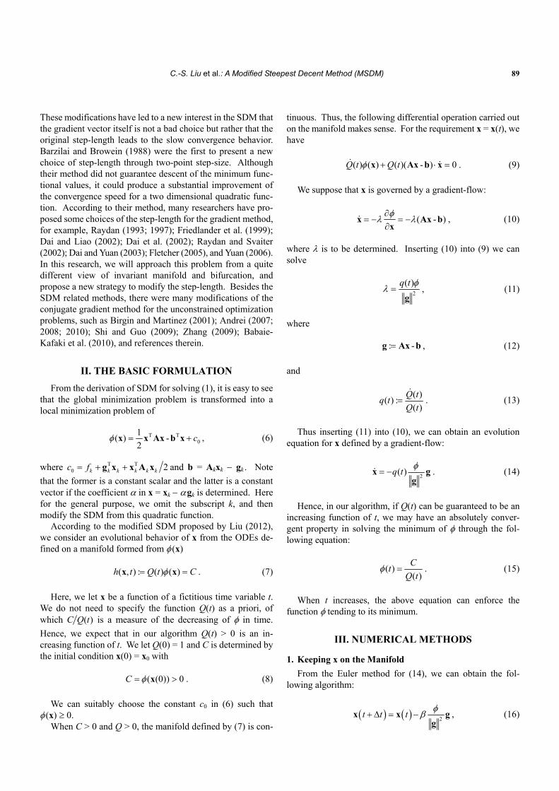
Fig. 2. For a Rosenbrock optimization problem the new algorithm is one

hundred times faster than the classical steepest descent method.

or Rosenbrock’s banana function. The minimum is zero oc-curring at (x1, x2) = (1, 1). This function is difficult to mini-mize because it has a steep sided valley following the para-

bolic curve 21 2x x . Kuo et al. (2006) have used the particle

swarm method to solve this problem; however, the numerical procedures are rather complex. Liu and Atluri (2008) have applied a fictitious time integration method to solve the above problem under the constraints of x1 0 and x2 0, whose accuracy can reach to the fifth order.

We apply the MSDM to this problem starting at (2, 0.5) under a convergence criterion = 1010 or a maximum number 10000 of iterations. The SDM is run over 10000 steps without convergence as shown in Fig. 2 by solid lines for showing a0 and s, residual error and f. The SDM can reach a very ac-curate value of f with 4.95 1019. The MSDM with = 0.0005 converges very fast only with 94 steps, with a0, s, residual error and f shown in Fig. 2 by dashed lines. The

SDM moving very slowly along the valleyMSDM moving very fast along the valley

1.0

0.9

0.8

0.7

0.6

0.5

0.8 1.2 1.6 2.0x1

x 2

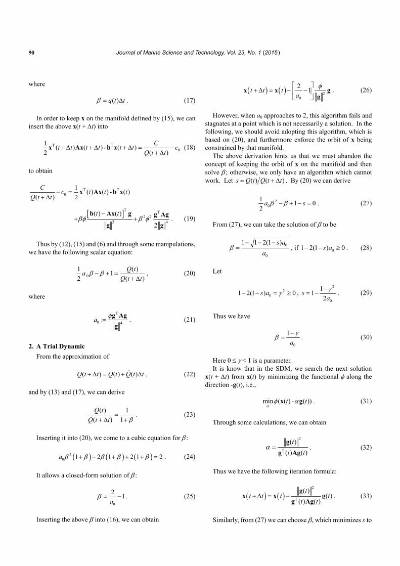
Fig. 3. For a Rosenbrock optimization problem comparing the iterative

paths of the SDM and the MSDM.

MSDM is 100 times faster than the SDM, and furthermore f can be reduced to 1.12 1023.

In Fig. 3, we compare the iterative paths generated by the SDM and the MSDM. It is found that both algorithms are fast approaching to the valley. In addition, when the SDM is mov-ing very slowly along the valley, the MSDM is moving very fast to the solution.

Now, we can explain the parameter appeared in (37). In Fig. 2(a), we compare a0 for = 0 and = 0.0005. It can be seen that for the case with = 0, the values of a0 tend to a constant and keep unchanged. By (21) it means that there exists an attracting set for the iterative orbit of x described by the following manifold:

0 4Constant

fa

Tg Ag

g. (40)

When the iterative orbit approaches to this manifold, the residual error is reduced slowly as shown in Fig. 2(c) by solid line, whereas the ratio of s is also keeping near to 1 as shown in Fig. 2(b) by the solid line. Conversely, for the case = 0.0005, a0 is no more tending to a constant as shown in Fig. 2(a) by the dashed line. Because the iterative orbit is not attracted by a constant manifold, the values of f as shown in Fig. 2(d) by the dashed line can be reduced step by step, whereas the ratio of s is often leaving the value near to 1 as shown in Fig. 2(b) by the dashed line. Thus, we can observe that when s varies from zero to a positive value, the iterative dynamics as given by (37) undergoes a Hopf bifurcation, like as the ODEs behavior ob-served by Liu (2000; 2007). The original stable manifold existent for = 0 now becomes a ghost manifold for = 0.0005,


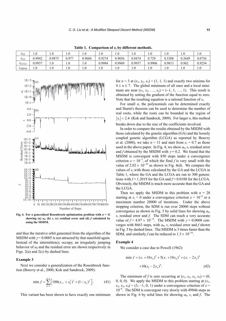
Table 1. Comparison of xi by different methods.

xEX 1.0 1.0 1.0 1.0 1.0 1.0 1.0 1.0 1.0 1.0 1.0 xGA 0.9942 0.9875 0.977 0.9604 0.9274 0.9056 0.8474 0.729 0.5308 0.2649 0.0756

xLCGA 0.9937 1.0 1.0 1.0 0.9984 0.9969 0.9937 0.9906 0.9813 0.962 0.9254

xMSDM 1.0 1.0 1.0 1.0 1.0 1.0 1.0 1.0 1.0 1.0 1.0

1E+3

1E+2

1E+1

1E+0

1E-1

4.0

2.0

0.0

-2.0

-4.0

(a)

(b)

(c)

(d)

a 0s

1E+01E+11E+21E+3

1E-11E-21E-31E-4

Res

idua

l Err

or

1E+01E+11E+21E+31E+4

1E-11E-21E-31E-41E-51E-61E-71E-81E-9

1E-10

850800750700650600550500450400350300250200150100500

f

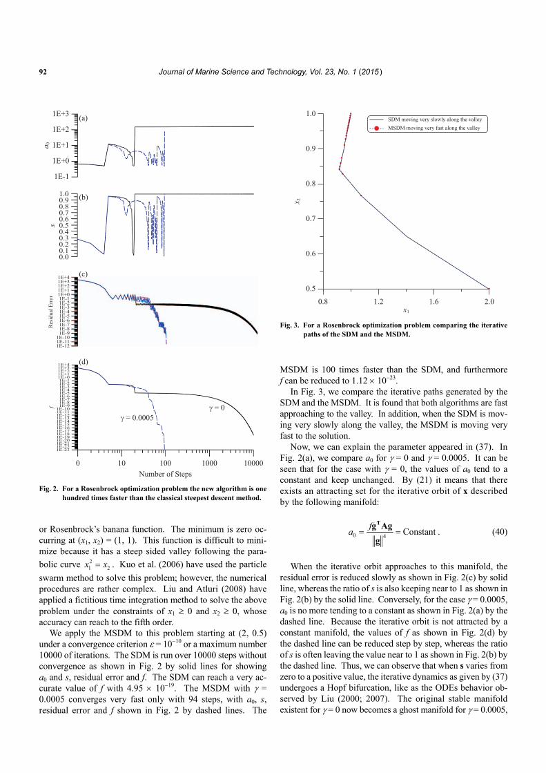
Number of Steps Fig. 4. For a generalized Rosenbrock optimization problem with n = 11

showing (a) a0, (b) s, (c) residual error and (d) f calculated by using the MSDM.

and thus the iterative orbit generated from the algorithm of the MSDM with = 0.0005 is not attracted by that manifold again. Instead of the intermittency occupy, an irregularly jumping behavior of a0 and the residual error are shown respectively in Figs. 2(a) and 2(c) by dashed lines.

Example 3

Next we consider a generalization of the Rosenbrock func-tion (Bouvry et al., 2000; Kok and Sandrock, 2009):

1

12 2 2

1

min 100( ) (1 )k

n

k kk

f x x x

. (41)

This variant has been shown to have exactly one minimum

for n = 3 at (x1, x2, x3) = (1, 1, 1) and exactly two minima for 4 n 7. The global minimum of all ones and a local mini-mum are near (x1, x2, , xn) = (1, 1, , 1). This result is obtained by setting the gradient of the function equal to zero. Note that the resulting equation is a rational function of xi.

For small n, the polynomials can be determined exactly and Sturm's theorem can be used to determine the number of real roots, while the roots can be bounded in the region of

2.4ix (Kok and Sandrock, 2009). For larger n, this method

breaks down due to the size of the coefficients involved. In order to compare the results obtained by the MSDM with

those calculated by the genetic algorithm (GA) and the loosely coupled genetic algorithm (LCGA) as reported by Bouvry et al. (2000), we take n = 11 and start from xi = 0.7 as those used in the above paper. In Fig. 4, we show a0, s, residual error and f obtained by the MSDM with = 0.2. We found that the MSDM is convergent with 850 steps under a convergence criterion = 103, of which the final f is very small with the value of 2.02 1010 as shown in Fig. 4(d). We compare the values of xi with those calculated by the GA and the LCGA in Table 1, where the GA and the LCGA are run to 300 genera-tions with f = 1.2019 for the GA and f = 0.0188 for the LCGA. Obviously, the MSDM is much more accurate than the GA and the LCGA.

Then we apply the MSDM to this problem with n = 20 starting at xi = 0 under a convergence criterion = 108 or a maximum number 20000 of iterations. Under the above stopping criterion, the SDM is run over 20000 steps without convergence as shown in Fig. 5 by solid lines for showing a0, s, residual error and f. The SDM can reach a very accurate value of f = 4.97 1015. The MSDM with = 0.0008 con-verges with 8663 steps, with a0, s, residual error and f shown in Fig. 5 by dashed lines. The MSDM is 3 times faster than the SDM, and similarly f can be reduced to 1.3 1016.

Example 4

We consider a case due to Powell (1962):

1 3 22 2 4

2 4 3min ( 10 ) 5( 10 ) ( 2 )f x x x x x x

41 410( 2 ) .x x (42)

The minimum of f is zero occurring at (x1, x2, x3, x4) = (0, 0, 0, 0). We apply the MSDM to this problem starting at (x1, x2, x3, x4) = (3, 1, 0, 1) under a convergence criterion of = 108. The SDM is convergent very slowly with 49846 steps as shown in Fig. 6 by solid lines for showing a0, s, and f. The


1E+3

1E+2

1E+1

1E+0

1E-1

1E-2

a 0

(a)

(b)

-18.0-16.0-14.0-12.0-10.0

-8.0-6.0-4.0-2.00.02.04.06.0

s

(c)1E+31E+21E+11E+01E-11E-21E-31E-41E-51E-61E-71E-81E-9

Res

idua

l Err

or

(d)1E+21E+11E+01E-11E-21E-31E-41E-51E-61E-71E-81E-9

1E-101E-111E-121E-131E-141E-151E-16

f

20000150001000050000Number of Steps

γ = 0

γ = 0.0008

Fig. 5. For a generalized Rosenbrock optimization problem with n = 20

the new algorithm is three times faster than the classical steepest descent method.

SDM can reach a very accurate value of f = 107. At the same time, the MSDM with = 0.15 converges with 1301 steps, with a0, s, and f shown in Fig. 6 by dashed lines. The MSDM is 38 times faster than the SDM, and furthermore we can get a more accurate f = 9.96 109.

Example 5

In this example, we design an office block inside a structure with a curved roof given by x = 100 y2. Suppose that the number of total cuboids is n and each cuboid can have dif-ferent size. We attempt to find the dimensions of all cuboids with maximum volume which would fit inside the given roof structure, that is,

2 21 1 2 1 2max 100 100 ( )f y y y y y

21100 ( ) ,n ny y y (43)

1E+51E+41E+31E+21E+11E+01E-1

a 0

(a)

(b)

0.30.40.50.60.70.80.91.0

s

(c)1E+21E+3

1E+11E+01E-11E-21E-31E-41E-51E-61E-71E-81E-9

f

500004000030000200000 10000Number of Steps

γ = 0γ = 0.15

Fig. 6. For the Powell case comparing (a) a0, (b) s and (c) f obtained by

the SDM and the MSDM.

where y1 > 0 is the height of the i-th cuboid.

The maximum of f is tending to 2000/3 when n is increasing. When n = 95, we apply the MSDM to this problem starting at yi = 0.05 under a convergence criterion of = 105. The SDM is convergent with 6868 steps as shown in Fig. 7 by solid lines for showing a0, s, residual error and f. At the same time, the MSDM with = 0.35 converges with 502 steps, with a0, s, residual error and f shown in Fig. 7 by dashed lines. Both f of the SDM and the MSDM are tending to 661.9945. The MSDM is 13 times faster than the SDM. The heights and widths of the cuboids with respect to the number of floors are plotted in Fig. 8.

Example 6

In this example, we design an office block inside a structure

with a circular roof given by 21296x y . Here we fix

n = 95, and consider

2 21 2 1 2max 1296 1296 ( )f y y y y y

211296 ( ) .n ny y y (44)

This problem is more difficult than that in Example 5.


1E+31E+21E+11E+0

1E+41E+51E+61E+71E+81E+9

1E+101E+111E+121E+131E+141E+151E+16

1E-1

a 0

(a)

(b)

0.2

0.4

0.6

0.8

1.0

s

(d)7E+2

6E+2

5E+2

4E+2

f

100001000100101Number of Steps

(c)1E+31E+21E+11E+01E-11E-21E-31E-41E-51E-6

Res

idua

l Err

or

γ = 0

γ = 0.35

Fig. 7. For the maximum area under a given curve comparing (a) a0, (b) s,

(c) residual error and (d) f obtained by the SDM and the MSDM.

100

80

60

40

20

0

Num

ber o

f Flo

ors

0.0 0.1 0.2 0.3 0.4 0 20 40 60 80 100Height Width

Fig. 8. Showing the heights and widths of the floors with respect to the number of floors

The maximum of f is tending to 324 = 1017.88 when n is

increasing. We apply the MSDM to this problem starting at yi = 1 under a convergence criterion of = 103. The SDM is

1E+31E+41E+51E+61E+7

1E+101E+11

1E+81E+9

1E+21E+11E+01E-1

a 0

(a)

(b)

0.0

0.2

0.4

0.6

0.8

1.0

s

(d)2E+32E+32E+32E+31E+31E+31E+31E+31E+3

6E+27E+28E+29E+2

f

25002000150010005000-500Number of Steps

(c)1E+31E+21E+11E+01E-11E-21E-31E-4

Res

idua

l Err

or

γ = 0

γ = 0.3

Fig. 9. For the maximum area under a circular roof comparing (a) a0,

(b) s, (c) residual error and (d) f obtained by the SDM and the MSDM.

convergent with 2358 steps as shown in Fig. 9 by solid lines for showing a0, s, residual error and f. At the same time, the MSDM with = 0.3 converges with 356 steps, with a0, s, residual error and f shown in Fig. 9 by dashed lines. Each f of the two methods is tending to 994.2315. The MSDM is 7 times faster than the SDM. The heights and widths of the cuboids with respect to the number of floors are plotted in Fig. 10.

Example 7

In this example, we test the minimization of the Schwefel function with n = 100:

2

1 1

minn i

ji j

f x

. (45)


20

16

12

8

4

0

Num

ber o

f Flo

ors

0 1 2 3 54 0 5 10 15 20 25 30 35Height Width

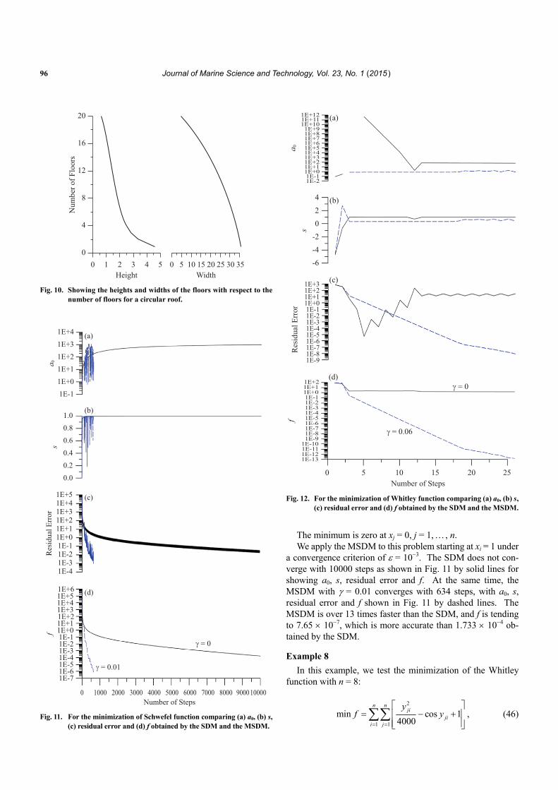
Fig. 10. Showing the heights and widths of the floors with respect to the number of floors for a circular roof.

1E+31E+4

1E+21E+11E+01E-1

a 0

(a)

(b)

0.00.20.40.60.81.0

s

(c)1E+51E+41E+31E+21E+11E+01E-11E-21E-31E-4

Res

idua

l Err

or

(d)1E+6

1E+2

1E+51E+41E+3

1E+11E+01E-11E-21E-31E-41E-51E-61E-7

f

100001000 2000 3000 4000 5000 6000 7000 8000 90000Number of Steps

γ = 0

γ = 0.01

Fig. 11. For the minimization of Schwefel function comparing (a) a0, (b) s,

(c) residual error and (d) f obtained by the SDM and the MSDM.

1E+121E+111E+10

1E+91E+8

1E+31E+21E+11E+0

1E+71E+61E+51E+4

1E-11E-2

a 0

(a)

(b)

-6-4-2024

s

(c)1E+31E+21E+11E+01E-11E-21E-31E-41E-51E-61E-71E-81E-9

Res

idua

l Err

or

(d)1E+21E+11E+01E-11E-21E-31E-41E-51E-61E-71E-81E-9

1E-101E-111E-121E-13

f

2515 201050Number of Steps

γ = 0

γ = 0.06

Fig. 12. For the minimization of Whitley function comparing (a) a0, (b) s,

(c) residual error and (d) f obtained by the SDM and the MSDM. The minimum is zero at xj = 0, j = 1, , n. We apply the MSDM to this problem starting at xi = 1 under

a convergence criterion of = 103. The SDM does not con-verge with 10000 steps as shown in Fig. 11 by solid lines for showing a0, s, residual error and f. At the same time, the MSDM with = 0.01 converges with 634 steps, with a0, s, residual error and f shown in Fig. 11 by dashed lines. The MSDM is over 13 times faster than the SDM, and f is tending to 7.65 107, which is more accurate than 1.733 104 ob-tained by the SDM.

Example 8

In this example, we test the minimization of the Whitley function with n = 8:

2

1 1

min cos 14000

n nji

jii j

yf y

, (46)


where 2 2 2100( ) ( 1)ji i j jy x x x . The minimum is zero at

xj = 1, j = 1, , n. It is very difficult to optimize. We apply the MSDM to this

problem starting at xi = 1.12 under a convergence criterion of = 108. The SDM diverges as shown in Fig. 12 by solid lines for showing a0, s, residual error and f. At the same time, the MSDM with = 0.06 converges with 26 steps, with a0, s, residual error and f shown in Fig. 12 by dashed lines, and f is tending to 1.54 1013. It can be found that the SDM fails.

V. CONCLUSIONS

By embedding the minimization problem into a continuous manifold with a fictitious time, we can derive a governing ODE for the unknown vector. Then by employing the Euler scheme, we have derived an iterative algorithm, which is naturally rendered to a modification of the classical steepest descent method (SDM) with a critical parameter 0 < 1. This novel algorithm might be named a modified steepest descent method (MSDM). We have proved that the minimi-zations in the SDM and in our formulation lead to the same algorithm, and are not the best ones, which usually result in a quite slow convergence of finding solution. The parameter is a bifurcation parameter, which played the role to change the situation from a slow convergence with = 0 to a quick con-vergence with > 0. This bifurcation is indeed an intermittent chaos which destabilizes the original invariant manifold ex-istent for = 0 in the SDM algorithm and is also the main reason to cause a slow convergence of the SDM for solving optimization problems. Through several tests, we have found that the MSDM outperforms very well as compared with the SDM.

ACKNOWLEDGMENTS

The corresponding and second authors would like to ex-press their thanks to the National Science Council of ROC for their financial support under contract number NSC 102-2218- E-019-001 and NSC-99-2221-E-019-053-MY3.

REFERENCES

Andrei, N. (2007). Scaled conjugate gradient algorithms for unconstrained optimization. Computational Optimization and Applications 38, 401-416.

Andrei, N. (2008). A Dai-Yuan conjugate gradient algorithm with sufficient descent and conjugacy conditions for unconstrained optimization. Ap-plied Mathematics Letters 21, 165-171.

Andrei, N. (2010). New accelerated conjugate gradient algorithms as a modifi-cation of Dai-Yuan’s computational scheme for unconstrained optimization. Journal of Computational and Applied Mathematics 234, 3397-3410.

Babaie-Kaffaki, S., R. Ghanbari and N. Mahdavi-Amiri (2010). Two new conjugate gradient methods based on modified secant equations. Journal

of Computational and Applied Mathematics 234, 1374-1386. Barzilai, J. and J. M. Borwein (1988). Two point step size gradient methods.

IMA Journal of Numerical Analysis 8, 141-148. Birgin, E. G. and J. M. Martinez (2001). A spectral conjugate gradient method

for unconstrained optimization. Applied Mathematics & Optimization 43, 117-128.

Bouvry, P., F. Arbab and F. Seredynski (2000). Distributed evolutionary opti-mization, in manifold: Rosenbrock’s function case study. Information Computer Science 122, 141-159.

Dai, Y. H. and L. H. Liao (2002). R-linear convergence of the Barzilai and Borwein gradient method. IMA Journal of Numerical Analysis 22, 1-10.

Dai, Y. H., J. Y. Yuan and Y. Yuan (2002). Modified two-point stepsize gra-dient methods for unconstrained optimization. Computational Optimiza-tion and Applications 22, 103-109.

Dai, Y. H. and Y. Yuan (2003). Alternate minimization gradient method,” IMA Journal of Numerical Analysis 23, 377-393.

Fletcher, R (2005). On the Barzilai-Borwein gradient method. In: Optimiza-tion and Control with Applications, edited by L. Qi, K. Teo and X. Yang, Springer, New York, 235-256.

Friedlander, A., J. M. Martinez, B. Molina and M. Raydan (1999). Gradient method with retards and generalizations. SIAM Journal on Numerical Analysis 36, 275-289.

Kok, S. and C. Sandrock (2009). Locating and characterizing the stationary points of the extended Rosenbrock function. Evolutionary computation 17, 437-453.

Kuo, H. C., J. R. Chang and C. H. Liu (2006). Particle swarm optimization for global optimization problems. Journal of Marine Science and Technology 14, 170-181.

Liu, C. S. (2000). Intermittent transition to quasi periodicity demonstrated via a circular differential equation. International Journal of Non-Linear Me-chanics 35, 931-946.

Liu, C. S. (2007). A study of type I intermittency of a circular differential equation under a discontinuous right-hand side. Journal of Mathematical Analysis and Applications, 331, 547-566.

Liu, C. S. (2012). Modifications of steepest descent method and conjugate gradient method against noise for ill-posed linear system. Communica-tions in Numerical Analysis 1, Doi: 10.5899/2012/can-00115.

Liu, C. S. and S. N. Atluri (2008). A fictitious time integration method (FTIM) for solving mixed complementarity problems with applications to non-linear optimization. CMES: Computer Modeling in Engineering and Sciences 34, 155-178.

Powell, M. J. D. (1962). An iterative method for finding stationary values of a function of several variables. The Computer Journal 5, 147-151.

Raydan, M. (1993). On the Barzilai and Borwein choice of step length for the gradient method. IMA Journal of Numerical Analysis 13, 321-326.

Raydan, M. (1997). The Barzilai and Borwein gradient method for the large scale unconstrained minimization problem. SIAM Journal on Optimiza-tion 7, 26-33.

Raydan, M. and B. F. Svaiter (2002). Relaxed steepest descent and Cauchy- Barzilai-Borwein method. Computational Optimization and Applications 21, 155-167.

Rosenbrock, H. H. (1960). An automatic method for finding the greatest or least value of a function. The Computer Journal 3, 175-184.

Shi, Z. J. and J. Guo (2009). A new family of conjugate gradient methods. Journal of Computational and Applied Mathematics 224, 444-457.

Yuan, Y. (2006). A new step size for the steepest descent method. Journal of Computational Mathematics 24, 149-156.

Zhang, L. (2009). A new Liu-Storey type nonlinear conjugate gradient method for unconstrained optimization problems. Journal of Computational and Applied Mathematics 225, 146-157.

a modified algorithm of steepest descent method for solving unconstrained … · 2016-01-29 · a...

Documents