a modiﬁed finite newton method for fast solution...

Journal of Machine Learning Research 6 (2005) 341-361 Submitted 11/04; Published 03/05

A Modified Finite Newton Method for Fast Solutionof Large Scale Linear SVMs

S. Sathiya Keerthi SATHIYA [email protected]

Dennis DeCoste [email protected]

Yahoo! Research Labs210 South Delacey AvenuePasadena, CA 91105, USA

Editor: Thorsten Joachims

Abstract

This paper develops a fast method for solving linear SVMs with L2 loss function that is suited forlarge scale data mining tasks such as text classification. This is done by modifying the finite Newtonmethod of Mangasarian in several ways. Experiments indicate that the method is much faster thandecomposition methods such as SVMlight, SMO and BSVM (e.g., 4-100 fold), especially whenthe number of examples is large. The paper also suggests waysof extending the method to otherloss functions such as the modified Huber’s loss function andthe L1 loss function, and also forsolving ordinal regression.

Keywords: linear SVMs, classification, conjugate gradient

1. Introduction

Linear SVMs (SVMs whose feature space is the same as the input space ofthe problem) are power-ful tools for solving large-scale data-mining tasks such as those arising in the textual domain. Quiteoften, these large-scale problems have a large number of examples as wellas a large number offeatures and the data matrix is very sparse (e.g.>99.9% sparse “bag of words” in text classifica-tion). In spite of their excellent accuracy, SVMs are sometimes not preferred because of the hugetraining times involved (Chakrabarti et al., 2003). Thus, it is important to have fast algorithms forsolving them. Traditionally, linear SVMs have been trained using decompositiontechniques suchas SVMlight (Joachims, 1999), SMO (Platt, 1999), and BSVM (Hsu and Lin, 2002), which solvethe dual problem by optimizing a small subset of the variables in each iteration.Each iteration costsO(nnz) time, wherennz is the number of non-zeros in the data matrix (nnz = mn if the data matrix isfull wherem is the number of examples andn is the number of features). The number of iterations,which is a function ofmand the number of support vectors, tends to grow super-linearly withmandthus these algorithms can be inefficient whenm is large.

With SVMs two particular loss functions for imposing penalties on slacks (violations on thewrong side of the margin, usually denoted byξ) have been popularly used.L1-SVMs penalizeslacks linearly (penalty=ξ) while L2-SVMs penalize slacks quadratically (penalty=ξ2/2). Thoughboth SVMs give good generalization performance,L1-SVMs are more popularly used because theyusually yield classifiers with a much less number of support vectors, thus leading to better classifi-cation speed. For linear SVMs the number of support vectors is not a matterof much concern since

c©2005 Sathiya Keerthi and Dennis DeCoste.

KEERTHI AND DECOSTE

the final classifier is directly implemented using the weight vector in feature space. In this paper wefocus onL2-SVMs.

Since linear SVMs are directly formulated in the input space, it is possible andworthwhileto think of direct methods of solving the primal problem without using the kernel trick. Primalapproaches are attractive because they assure a continuous decrease in the primal objective function.

Recently some promising primal algorithms have been given for training linear classifiers. Fungand Mangasarian (Fung and Mangasarian, 2001) have given a primalversion of the least squaresformulation of SVMs given by Suykens and Vandewalle (1999). Komarek(2004) has effectivelyapplied conjugate gradient schemes to logistic regression. Zhang et al. (2003) have given an indirectalgorithm for linearL1-SVMs that works by approximating theL1 loss function by a sequenceof smooth modified logistic regression loss functions and then sequentially solving the resultingsmooth primal modified logistic regression problems by nonlinear conjugate gradient methods. Aparticular drawback of that method is its inability to exploit the sparsity propertyof SVMs: thatonly the support vectors determine the final solution.

A direct primal algorithm forL2-SVMs that exploits the sparsity property, called the finite New-ton method, was given by Mangasarian (2002). It was mainly presented for problems in whichthe number of features is small. The main aim of this paper is to introduce appropriate tools thattransform this method into a powerfully fast technique for solving large scale data mining problems(with a large number of examples and/or a large number of features). Our main contributions are:(1) we modify the finite Newton method by keeping the least squares nature ofthe problem intact ineach iteration and using exact line search; (2) we bring in special, numerically robust conjugate gra-dient techniques to implement the Newton iterations; and (3) we introduce heuristics that speed-upthe baseline implementation considerably. The result is an algorithm that is numerically robust andvery fast. An attractive feature of the algorithm is that it is also very easy toimplement; AppendixA gives a pseudocode that can be easily transcribed into a working code.

We show that the method that we develop forL2-SVMs can be extended in a straight-forwardway to the modified Huber’s loss function (Zhang, 2004) and, in a slightly more complicated wayto theL1 loss function. We also show how the algorithm can be modifed to solve ordinalregression.

The paper is organized as follows. Section 2 formulates the problem and gives basic results.The modified finite Newton algorithm is developed in Section 3. Section 4 gives full details associ-ated with a practical implementation of this algorithm. Section 5 gives computational experimentsdemonstrating the efficiency of the method in comparison with standard methods such as SVMlight

(Joachims, 1999) and BSVM (Hsu and Lin, 2002). Section 6 suggests ways for extending themethod to other loss functions and Section 7 explains how ordinal regression can be solved. Section8 contains some concluding remarks.

2. Problem Formulation and Some Basic Results

Consider a binary classification problem with training examples,{xi , ti}mi=1 wherexi ∈ Rn andti ∈

{+1,−1}. To obtain a linear classifiery = w·x+b, L2-SVM solves the following primal problem:

min(w,b)

12(‖w‖2 +b2)+

C2

m

∑i

ξ2i s.t. ti(w·xi +b) ≥ 1−ξi ∀ i (1)

whereC is the regularization parameter. We have included theb2/2 term so that standard regularizedleast squares algorithms can be used directly. Our experience shows that generalization performance

342

FINITE NEWTON METHOD FOR LINEARSVMS

is not affected by this inclusion. In a particular problem if there is reason tobelieve that the addedterm does affect performance, one can proceed as follows: takeγ2b2/2 as the term to be included;then defineb = γb as the new bias variable and take the classifier to bey = w · x+ (1/γ)b. Theparameterγ can either be chosen to be a small positive value or be tuned by cross validation.

For applying least squares ideas neatly, it is convenient to transform (1) to an equivalent formu-lation by eliminating theξi ’s and dividing the objective function by the factorC. This gives1

minβ

f (β) =λ2‖β‖2 +

12 ∑

i∈I(β)

d2i (β) (2)

whereβ = (w,b), λ = 1/C, di(β) = yi(β)− ti , yi(β) = w·xi +b, andI(β) = {i : tiyi(β) < 1}.Least Squares SVM (LS-SVM) (Suykens and Vandewalle, 1999) corresponds to (1) with the

inequality constraints replaced by the equality constraints,ti(w · xi + b) = 1− ξi for all i. Whentransformed to the form (2), this is equivalent to settingI(β)={1, . . . ,m}; thus, LS-SVM is solvedvia a single regularized least squares solution. In contrast, the dependance ofI(β) onβ complicatestheL2-SVM solution. In spite of this complexity, it can be advantageous to opt for usingL2-SVMsbecause they do not allow well-classified examples to disturb the classifier design. This is especiallytrue in problems where the support vectors are a small subset of all examples.2

Let us now review several basic results concerningf , some of which are given in Mangasarian(2002). First note thatf is a piecewise quadratic function. The presence of theλ‖β‖2/2 term makesf strictly convex. Thus it has a unique minimizer.f is continuously differentiable in spite of thejumps inI(β), the reason for this being that when an indexi causes a jump inI(β) at someβ, its di

is 0. The gradient off is given by

∇ f (β) = λβ+ ∑i∈I(β)

di(β)

(

xi

1

)

. (3)

Given an index setI ⊂ {1, . . . ,m}, let us define the functionfI as

fI (β) =λ2‖β‖2 +

12 ∑

i∈I

d2i (β). (4)

Clearly fI is a strictly convex quadratic function and so it has a unique minimizer. It follows directlyfrom (3) that, for anyβ, ∇ f (β)|β=β = ∇ fI (β)|β=β whereI = I(β). In fact, there exists an open set

aroundβ in which f and fI are identical. It follows thatβ minimizes f iff it minimizes fI .

3. The Modified Finite Newton Algorithm

Mangasarian’s finite newton method (Mangasarian, 2002) does iterationsof the form

βk+1 = βk +δkpk,

1. To help see the equivalence of (1) and (2), note that at a given(w,b), the minimization ofξ2i in (1) will automatically

chooseξi = 0 for all i 6∈ I(β).2. We find thatL2-SVMs usually achieve better generalization performance over LS-SVMs. Interestingly, we also find

L2-SVMs often train faster than LS-SVMs, due to sparseness arising fromsupport vectors.

343

KEERTHI AND DECOSTE

where the search directionpk is based on a second order approximation of the objective function atβk:

pk = −H(βk)−1∇ f (βk).

Since f is not twice differentiable atβ where at least one of thedi is zero,H(β) is taken to bethe generalized Hessian defined byH(β) = λJ+CTDC whereJ is then×n identity matrix,C is amatrix whose rows are(xT

i ,1) andD is a diagonal matrix whose diagonal elements are given by:

Dii =

1 if tiyi(β) < 1some specific element of[0,1] if tiyi(β) = 10 if tiyi(β) > 1

(5)

Note that examples with indices satisfyingtiyi(β) > 1 do not affectH(β) and pk. (This propertycontributes greatly to the overall efficiency of the method.) The step sizeδk is chosen to satisfy anArmijo condition that ensures convergence, and it is found by applying a halving method of linesearch in the[0,1] interval. (IfC in (1) is sufficiently small then it is shown in Mangasarian (2002)that the fixed step size,δk = 1 suffices for convergence.)

We modify the algorithm slightly in two ways. First, we avoid doing anything special for caseswheretiyi(β) = 1 occurs. (Essentially, we setDii = 0 in (5) for such cases.) This lets us keep the leastsquares nature of the problem intact. More precisely, instead of computingthe Newton directionpk, we compute the Newton point,βk + pk, which is the solution of a regularized least squaresproblem. As we will see in the next section, this has useful implications on stablealgorithmicimplementation. Second, we do an exact line search to determineδk. This feature allows us todirectly apply convergence results from nonlinear optimization theory. (Inthe next section we givea fast method for exact line search.) Thus, at one iteration, given a point β we setI = I(β) andminimize fI to obtain the Newton point,β. Then an exact line search on the ray fromβ to βyields the next point of the method. These iterations are repeated till the algorithm converges. Theoverall algorithm is given below. Implementation details associated with each step are discussed inSection 4.

344


Algorithm L2-SVM-MFN.

1. Choose a suitable startingβ0. Setk = 0 and go to step 2.

2. Check ifβk is the optimal solution of (2). If so, stop withβk as the solution. Else go to step 3.

3. Let Ik = I(βk). Solvemin

βfIk(β). (6)

Let β denote the solution obtained.

4. Do a line search to decrease the “full” objective function,f :

minβ∈L

f (β), (7)

whereL = {β = βk + δ(β−βk) : δ ≥ 0}. Let δ? denote the solution of this line search. Setβk+1 = βk +δ?(β−βk), k := k+1 and go back to step 2 for another iteration.

Theorem 1. Algorithm L2-SVM-MFN converges to the solution of (1) in a finite number ofiterations.

Proof. Let pk = (β − βk). Note thatpk = −H−1Ik

∇ f (βk) and λI ≤ HIk ≤ Hall whereHIk isthe Hessian offIk andHall is the Hessian off{1,...,m}. By Proposition 1.2.1 of Bertsekas (1999) itfollows3 that {βk} converges to the minimizer off . Proof of finite convergence is exactly as inMangasarian’s proof of finite convergence of his algorithm, and goes as follows. Letβ? denote theminimizer of f andI? = I(β?). Let O = {β : I(β) = I?}. ClearlyO is an open set that containsβ?.Since{βk} converges toβ?, there exists ak such thatβk ∈ O. When this happens in step 2 of thealgorithm, we getβ = β? in step 3 and soβk+1 = β?.

4. Practical Implementation

In this section we discuss details associated with the implementation of the various steps of themodified finite Newton algorithm and also introduce some useful heuristics forspeeding up thealgorithm. The discussion leads to a fast and robust implementation ofL2-SVM-MFN. The fi-nal algorithm is also very easy to implement; Appendix A gives a pseudocodethat can be easilytranscribed into a working code. A number of data sets are used in this section to illustrate theeffectiveness of various implementation features. These data sets are described in Appendix B. Allour computations were done on a 2.4 GHz machine with Intel Xeon processorand having four GbRAM.

4.1 Step 1: Initialization

If no guess ofβ is available, then the simplest starting point isβ0 = 0. For this point we haveyi = 0for all i and soI0 = {1, . . . ,m}. Therefore, with such a zero initialization, theβ obtained in step 3 isexactly the LS-SVM solution.

3. To apply Proposition 1.2.1 of Bertsekas (1999) note the following: (a) Becauseλ > 0 andHall is positive definite,condition (1.12) of Bertsekas (1999) holds; (b) Bertsekas (1999) shows that (1.12) implies (1.13) given there; (c) inBertsekas (1999) exact line search is referred as the minimization rule.

345

KEERTHI AND DECOSTE

Adult-9 Web-8 News20 Financial YahooNo β-seeding 60.26 105.16 1321.87 1130.35 11650.56

β-seeding 36.80 24.43 944.27 692.47 4419.89

Table 1: Effectiveness ofβ-seeding on five data sets. The following 21C values were used:√

2k,

k = −10,−9, . . . ,9,10. All computational times are in seconds.

Suppose we have a guess ˜w for the weight vectorw. It is possible that ˜w comes from an in-expensive classification method, such as the Naive-Bayes classifier. In that case it is necessary torescale ˜w and also chooseb0 so as to form aβ0 that is good for starting the SVM solution. So wesetβ0 = (γw,b0) and choose suitable values forγ andb0. Suppose we also assume thatI , a guess ofthe optimal set of active indices, is available. (If no guess is available, we can simply letI be the setof all training indices.) Then chooseγ andb0 to minimize the cost

λ2[γ2‖w‖2 +b2

0]+12 ∑

i∈I

[γw·xi +b0− ti ]2. (8)

It is easy to check that the resultingγ andb0 are given by

γ = (p22q1− p12q2)/d and b0 = (p11q2− p12q1)/d. (9)

where p11 = λ‖w‖2 + ∑i∈I (w · xi)2, p22 = λ + |I |, p12 = ∑i∈I w · xi , q1 = ∑i∈I tiw · xi , q2 = ∑i∈I ti

andd = p11p22− (p12)2. Onceγ andb0 are thus obtained, we can setβ0 = (γw,b0) and start the

algorithm.4 Note that the set of initial indicesI0 chosen by the algorithm in step 3 is the set of activeindices atβ0 and so it could be different fromI .

There is another situation where the above initialization comes in handy. Suppose we solve (2)for oneC and want to re-solve (2) for a slightly changedC. Then we can use the ˜w andI that areobtained from the optimal solution of the first value ofC to do the above mentioned initializationprocess for the second value ofC. For this situation we have also tried simply choosingγ = 1 andb0 equal to theb that is optimal for the first value ofC. This simple initialization also works quitewell. We will refer to this initialization for the ‘slightly changedC’ situation asβ-seeding; seedingis crucial to efficiency when (2) is to be solved for manyC values (such as when tuningC via cross-validation). Theβ-seeding idea used here is very much similar to the idea ofα-seeding popularlyemployed in the solution of SVM duals(DeCoste and Wagstaff, 2000).

Eventhough full details of the final version of our implementation ofL2-SVM-MFN is onlydeveloped further below, here let us compare the final implementation5 with and withoutβ-seeding.Table 1 gives computational times for several data sets. Clearly,β-seeding gives useful speed-ups.

4. To get a betterβ0 one can also resetI = I(β0) and repeat (9) and get revised values forγ andb0. This computation ischeap since ˜w ·xi need not be recomputed.

5. For noβ-seeding, the implementation corresponds to the use of ‘both heuristics’ mentioned in Table 3. Forβ-seeding,the two heuristics are not used since they do not contribute much whenβ-seeding is done.

346


4.2 Step 2: Checking Convergence

Checking of the optimality ofβk is done by first calculatingyi(βk) anddi(βk) for all i, determiningthe active index setIk and then checking if

‖∇ fIk(βk)‖ = 0. (10)

For practical reasons it is necessary to employ a tolerance parameter when checking (10). We dealwith this important issue below after the discussion of the implementation of step 3.

4.3 Step 3: Regularized Least Squares Solution

The solution of (6) can be approached in one of the following ways: usingfactorization methodssuch as QR or SVD; or, using an iterative method such as the conjugate gradient (CG) method. Weprefer the latter method due to the following reasons: (a) it can make effective use of knowledge ofgood starting vectors; and (b) it is much better suited for large-scale problems having sparse datasets. To setup the details of the CG method, let:X be the matrix whose rows are(xT

i ,1), i ∈ Ik;andt be a vector whose elements areti , i ∈ Ik. Then (6) is the same as the regularized least squaresproblem

minβ

fIk(β) =λ2‖β‖2 +

12‖Xβ− t‖2. (11)

This corresponds to the solution of the normal system,

(λI +XTX)β = XTt. (12)

With CG methods there are several ways of approaching the solution of (11/12). A simple approachis to solve (12) using the CG method meant for solving positive definite systems.However, suchan approach will not be numerically well-conditioned, especially whenλ is small. As pointed outby Paige and Saunders (Paige and Saunders, 1982) this is mainly due to theexplicit use of vectorsof the form XTX p. An algorithm with better numerical properties can be easily derived by analgorithmic rearrangement that is special to the regularized least squaressolution, which makes useof the intermediate vectorX p. LSQR (Paige and Saunders, 1982) and CGLS (Bjorck, 1996) are twosuch special CG algorithms. Another very important reason for using oneof these algorithms (asopposed to using a general purpose CG solver) is that, for the special methods it is easy to derive agood stopping criterion to approximately terminate the CG iterations using the intermediate residualvector. We discuss this issue in more detail below.

For our work we have used the version of the CGLS algorithm given in Algorithm 3 of Frommerand Maaß (Frommer and Maaß, 1999) which uses initial seed solutions neatly.6 Following is theCGLS algorithm for solving (11).

Algorithm CGLS. Setβ0 = βk (whereβk is as in steps 2 and 3 of AlgorithmL2-SVM-MFN).Computez0 = t −Xβ0, r0 = XTz0−λβ0,7 setp0 = r0 and do the following steps forj = 0,1, . . .

6. Frommer and Maaß have also given interesting variations of the CGLS method for efficiently solving (12) for severalvalues ofλ. But we have not tried those methods in this work.

7. It is useful to note that, at any point of the CGLS algorithm−zj is the vector containing the classifier residuals,di ,i ∈ Ik andr j is the negative of the gradient offIk(β) atβ j . At the beginning (j = 0), z0 andr0 are already available inview of the computations in step 2 of AlgorithmL2-SVM-MFN. This fact can be used to gain some efficiency.

347

KEERTHI AND DECOSTE

q j = X pj

γ j = ‖r j‖2/(‖q j‖2 +λ‖p j‖2)β j+1 = β j + γ j p j

zj+1 = zj − γ jq j

r j+1 = XTzj+1−λβ j+1

If r j+1 = 0 stop withβ j+1 as the solution.ω j = ‖r j+1‖2/‖r j‖2

p j+1 = r j+1 +ω j p j

There are exactly two matrix-vector operations in each iteration; sparsity ofthe data matrix canbe effectively used to do these operations inO(nz) time wherenz is the number of non-zero elementsin the data matrix.

Let us now discuss the convergence properties of CGLS. It is known that the algorithm willtake at mostl iterations wherel is the rank ofX. Note thatl ≤ min{m,n} wherem is the numberof examples andn is the number of features. The actual number of iterations required to achievegood practical convergence is usually much smaller than min{m,n} and it depends on the numberof singular values ofX that are really significant.

Stopping the CG iterations with the right accuracy is very important because, an excessivelyaccurate solution would lead to too much work while an inaccurate solution will not give gooddescent. Using a simple absolute tolerance on the size of the gradient offIk in order to stop is a badidea, even for a given data set since the typical size of the gradient varies a lot asλ is varied over arange of values. For a method such as CGLS it is easy to find effective practical stopping criteria.We can decide to stop when the negative gradient vectorr j+1 has come near zero up to some relativeprecision. To do this we can use the bound,‖r j+1‖ ≤ ‖X‖‖zj+1‖+‖λβ j+1‖. Thus a good stoppingcriterion is

‖r j+1‖ ≤ ε(ρ‖zj+1‖+λ‖β j+1‖),whereρ = ‖X‖. SinceX varies at different major iterations of theL2-SVM-MFN algorithm, we cansimply takeρ = ‖X‖ whereX is the entirem×n data matrix.

In most datamining tasks the data is normalized so that all values in the data matrix are in theunity range. For such data sets we have‖X‖ ≤ √

n. One can take a conservative approach andsimply use the stopping criterion

‖r j+1‖ ≤ ε‖zj+1‖. (13)

We have found this criterion to be very effective and have used it for allthe computational experi-ments reported in this paper. The parameterε is a relative tolerance parameter. A value ofε = 10−6,which roughly yields solutions accurate up to six decimal digits, is a good choice.

Sincer = −∇ fIk we can apply exactly the same criteria as in (13) for approximately checking(10) also. Almost always, termination ofL2-SVM-MFN occurs when, after the least squares solu-tion at step 3, exact line search in step 4 givesβk+1 = β (i.e., δ? = 1), and the active set remainsunchanged, i.e.,I(βk) = I(β) = I(βk+1).

Let us illustrate the effectiveness of the CGLS method using the LS-SVM solution as an ex-ample. For LS-SVM we can setI = {1, . . . ,m} and solve (12) using the CGLS method mentionedabove; let us refer to such an implementation as LS-SVM-CG. In their proximal SVM implemen-tation of LS-SVM, Fung and Mangasarian (2001) solve (12) using Matlabroutines that employfactorization techniques onXTX. For large and sparse data sets it is much more efficient to use CGmethods and avoid the formation ofXTX and its factorization. Table 2 illustrates this fact using two

348


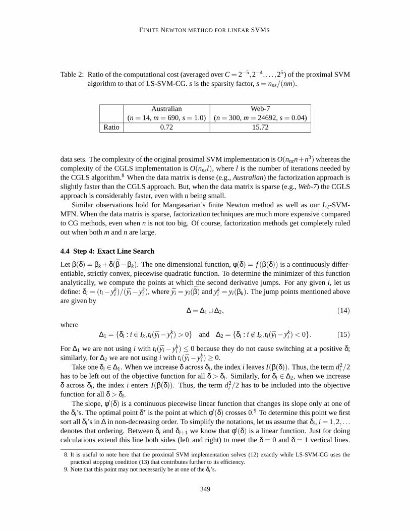
Table 2: Ratio of the computational cost (averaged overC = 2−5,2−4, . . . ,25) of the proximal SVMalgorithm to that of LS-SVM-CG.s is the sparsity factor,s= nnz/(nm).

Australian Web-7(n = 14,m= 690,s= 1.0) (n = 300,m= 24692,s= 0.04)

Ratio 0.72 15.72

data sets. The complexity of the original proximal SVM implementation isO(nnzn+n3) whereas thecomplexity of the CGLS implementation isO(nnzl), wherel is the number of iterations needed bythe CGLS algorithm.8 When the data matrix is dense (e.g.,Australian) the factorization approach isslightly faster than the CGLS approach. But, when the data matrix is sparse (e.g.,Web-7) the CGLSapproach is considerably faster, even withn being small.

Similar observations hold for Mangasarian’s finite Newton method as well as our L2-SVM-MFN. When the data matrix is sparse, factorization techniques are much more expensive comparedto CG methods, even whenn is not too big. Of course, factorization methods get completely ruledout when bothmandn are large.

4.4 Step 4: Exact Line Search

Let β(δ) = βk +δ(β−βk). The one dimensional function,φ(δ) = f (β(δ)) is a continuously differ-entiable, strictly convex, piecewise quadratic function. To determine the minimizer of this functionanalytically, we compute the points at which the second derivative jumps. Forany giveni, let usdefine:δi = (ti −yk

i )/(yi −yki ), where ¯yi = yi(β) andyk

i = yi(βk). The jump points mentioned aboveare given by

∆ = ∆1∪∆2, (14)

where∆1 = {δi : i ∈ Ik, ti(yi −yk

i ) > 0} and ∆2 = {δi : i 6∈ Ik, ti(yi −yki ) < 0}. (15)

For ∆1 we are not usingi with ti(yi − yki ) ≤ 0 because they do not cause switching at a positiveδ;

similarly, for ∆2 we are not usingi with ti(yi −yki ) ≥ 0.

Take oneδi ∈ ∆1. When we increaseδ acrossδi , the indexi leavesI(β(δ)). Thus, the termd2i /2

has to be left out of the objective function for allδ > δi . Similarly, for δi ∈ ∆2, when we increaseδ acrossδi , the indexi entersI(β(δ)). Thus, the termd2

i /2 has to be included into the objectivefunction for allδ > δi .

The slope,φ′(δ) is a continuous piecewise linear function that changes its slope only at one oftheδi ’s. The optimal pointδ? is the point at whichφ′(δ) crosses 0.9 To determine this point we firstsort allδi ’s in ∆ in non-decreasing order. To simplify the notations, let us assume thatδi , i = 1,2, . . .denotes that ordering. Betweenδi andδi+1 we know thatφ′(δ) is a linear function. Just for doingcalculations extend this line both sides (left and right) to meet theδ = 0 andδ = 1 vertical lines.

8. It is useful to note here that the proximal SVM implementation solves (12) exactly while LS-SVM-CG uses thepractical stopping condition (13) that contributes further to its efficiency.

9. Note that this point may not necessarily be at one of theδi ’s.

349

KEERTHI AND DECOSTE

Let us call the ordinate values at these two meeting points asl i andr i respectively. It is very easy tokeep track of the changes inl i andr i as indices get dropped and added to the active set of indices.

We move from left to right to find the zero crossing ofφ′(δ). At the beginning we are atδ0 = 0.Betweenδ0 andδ1 we haveIk as the active set. It is easy to get, from the definition ofφ(δ) that

l0 = λβk · (β−βk)+ ∑i∈Ik

(yki − ti)(yi −yk

i ) (16)

andr0 = λβ · (β−βk)+ ∑

i∈Ik

(yi − ti)(yi −yki ). (17)

(If, at step 3 of theL2-SVM-MFN algorithm, we solve (6) exactly, then it is easy to check thatr0 = 0. However, in view of the use of the approximate termination mentioned in (13) itis better tocomputer0 using (17).) Find the point where the line joining(0, l0) and(1, r0) points on the(δ,φ′)plane crosses zero. If the zero crossing point of this line is between 0 and δ1 then that point isδ?. Ifnot, we move over to searching betweenδ1 andδ2. Herel1 andr1 need to be computed. This canbe done by a simple updating overl0 andr0 since only the termd2

i /2 enters or leaves. Thus, for ageneral situation where we already havel i , r i computed for the intervalδi to δi+1 and we need to getl i+1, r i+1 for the intervalδi+1 to δi+2, we use the update formula

l i+1 = l i +s(yki − ti)(yi −yk

i ) and r i+1 = r i +s(yki − ti)(yi −yk

i ), (18)

wheres= −1 if δi ∈ ∆1 ands= 1 if δi ∈ ∆2. Thus we keep moving to the right until we get a zerosatisfying the condition that the root determined by interpolating(0, l i) and(1, r i) lies betweenδi

andδi+1. The process is bound to converge since we know the existence of the minimizer (we aredealing with a strictly convex function). In a typical application of the above line search algorithm,manyδi ’s are crossed beforeδ? is reached, especially in the early stages of the algorithm, causing|I(βk+1)| to be much different from|I(βk)|. This is the crucial step where the support vectors of theproblem get identified.

The complexity of the above exact line search algorithm isO(mlogm). Since the least squaressolution (step 3) is much more expensive, the cost of exact line search is negligible.

4.5 Complexity Analysis

The bulk of the cost of the algorithm is associated with step 3, which only dealswith examples thatare active at the current point. (The full set of examples is involved onlyin step 4.) This crucialfactor greatly contributes to the overall efficiency of the algorithm. The number of iterations, i.e.,loops of steps 2-4 is usually small, say 5-20. Thus, the empirical complexity ofthe algorithm isO(nnzlav) wherelav, the average number of CG iterations in step 3, is bounded by the rank of thedata matrix and solav ≤ min{m,n}. As already mentioned,lav usually turns out to be much smallerthan both,m andn. For example, when applied to thefinancialdata set that has 198788 examplesand 252472 features, forC = 1 andβ = 0 initialization, L2-SVM-MFN took 11 iterations, withlav = 102.

4.6 Speed-up Heuristics

Suppose we are solving a problem for which the number of support vectors, i.e.,|I(β?)| is a smallfraction ofm, and we use the initialization,β0 = 0. SinceI(β0) = {1, . . . ,m}, step 3 corresponds to

350


Adult-9 Web-8 News20 Financial YahooNo heuristics 7.28 11.79 98.06 456.85 1443.23Heuristic 1 5.12 9.24 67.85 70.86 904.99Heuristic 2 3.57 4.17 90.54 202.62 848.99

Both heuristics 3.00 3.90 52.73 62.18 524.16SV fraction 0.605 0.219 0.650 0.068 0.710

Table 3: Effectiveness of the two speed-up heuristics on five data sets.The valueC = 1 was used.All computational times are in seconds. SV fraction is the ratio of the number of supportvectors to the number of training examples.

solving an unnecessarily large least squares problem; it is wasteful to solve it accurately. One (orboth) of the following two heuristics can be employed to avoid this.

Heuristic 1. Wheneverβ0 is a crude approximation (say,β0 = 0), terminate the least squaressolution of (6) after a fixed, small number (say, 10) of CGLS iterations at the first call to step 3.Even with the crudeβ thus generated, the following step 4 usually leads to a pointβ1 with |I(β1)|much smaller thanm, and a good bulk of the non-support vectors get identified correctly.

Heuristic 2.First run theL2-SVM-MFN algorithm using a crude tolerance, sayε = 10−2. Usethe β thus generated as the starting vector and make another run withε = 10−6, the final desiredaccuracy.

Table 3 gives the effectiveness of the above heuristics on a few data sets. Clearly both heuristicsare useful. It is not easy to say which one is more effective and so usingboth of them is theappropriate thing to do. This gives at least a 2-fold speed-up. As expected, the amount of speed-upis big if the fraction of examples that are support vectors is small. The pseudocode of Appendix Buses both heuristics.

A third heuristic may also be used when working with a very large number of examples. Firstchoose a small random subset of the examples and run the algorithm. Then use theβ thus generatedto seed a second run, this time using all the examples for training.

We end this section on implementation by explaining how a solution of the SVM dual can beobtained afterL2-SVM-MFN solves the primal.

4.7 Obtaining a Dual Solution

Note that the SVM dual variables,αi , i = 1, . . . ,m are not involved anywhere in the algorithm. Butit is easy to recover them once we solve (2) usingL2-SVM-MFN. From the structure of (3) it iseasy to see thatαi = −tidi/λ, if i ∈ I(β) andαi = 0 otherwise. In a practical solution we do not getthe true solution due to the use of (13). In such a situation it is useful to ask as to how well theαdefined above satisfies the KKT optimality conditions of the dual. This can be easily done. Aftercomputingα as mentioned above, setβ = ∑i αiti(xT

i ,1)T , ξi = λαi ∀i, gi = tiyi(β)+ ξi −1 ∀i, andobtain the maximum dual KKT violation as max{maxi:αi>0 |gi |,maxi:αi=0max{0,−gi}}. If, keepingthe maximum dual KKT violation within some specified tolerance (say,τ = 0.001) is important forsome reason, then one can proceed as follows. First solveL2-SVM-MFN usingε = 10−3 and then

351

KEERTHI AND DECOSTE

check the maximum dual KKT violation as described above. If it does not satisfy the requiredtolerance then continue theL2-SVM-MFN solution with a suitably chosen smaller value ofε.

5. Comparison with SVMlight and BSVM

The experiments of this section compareL2-SVM-MFN against two dual-based methods: the pop-ular SVMlight (Joachims, 1999)10 and the more modern BSVM (Hsu and Lin, 2002). In order tomake a proper comparisonL2-SVM-MFN was forced to satisfy the same dual KKT tolerance ofτ = 0.001 as the other methods. (The procedure given at the end of the last section was used todo this.) We used default-q (subproblem size) for SVMlight & BSVM; other values tried werenot faster.11 We also tried SMO (Platt, 1999), but found it slower than the others for these linearproblems. An explanation for this is given by Kao et al (Kao et al., 2004) inSection 4 of their papervia the fact that, for the linear SVM implementation, the cost of updating the gradient of the dual isindependent of the number of dual variables that are optimized in each basic iteration.

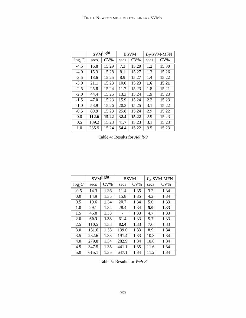
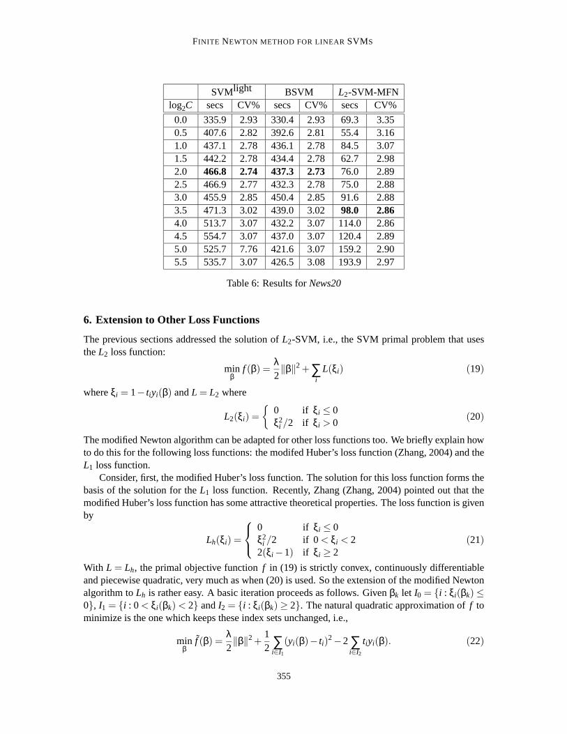
Tables 4-6 report training times and 10-fold cross-validation (CV) error rates forAdult-9, Web-8andNews20data sets.

We show training times for variousC’s, with optimal (lowest) mean CV error rate for eachmethod shown in bold. Due to the different loss functions used, a direct comparison of these meth-ods is challenging and necessarily approximate on non-separable data. Therefore, in the followingtables we show results for a range ofC values around values ofC yielding minimum cross-validationerrors for each of the three methods. A reasonable conservative speedup for our method can then bedetermined by selecting the slowest training time for a near-optimalC value for our method versusthe fastest training time for a near-optimalC value for an alternative method.

For example, forAdult-9one could compare the time for SVMlight’s CV-optimal (112.6 secs)versus the time forL2-SVM-MFN’s CV-optimal (1.6 secs), yielding a speedup ratio of 70.4. Al-ternatively,nearly-CV-optimal cases forAdult-9(e.g. 15.23%>15.22% for SVMlight with C=2−3)yield other speedups (e.g. 13.2 if both SVMlight andL2-SVM-MFN useC=2−3). Over all suchnearly-optimal cases for all three data sets, speedups are consistently significant (e.g. 4-100 overSVMlight and 4-40 over BSVM). Even forNews20which has more than a million features12 L2-SVM-MFN is more than four times faster than SVMlight and BSVM.

For theYahoodata set having a million examples, SVMlight and BSVM could not completethe solution even after one full day, whileL2-SVM-MFN took only about 10 minutes to obtain asolution.

We also did an experiment to study how the algorithms scale withm, the number of examples.Figure 1 gives log-log plots showing the variation of training times as a functionof m, for four of theconventionalAdult andWebsubsets. The times plotted for each data subset/method pair are for thecorresponding CV-optimalC’s. These plots show that not only wasL2-SVM-MFN always faster,but it also scaled much better withm.

10. We report results using version 5.0 of SVMlight. We also tried the newer version 6.0, but found for our particularexperiments with linear kernels that it was no faster, and sometimes even slower.

11. Specifically, the values used forq were 10 for SVMlight and 30 for BSVM.

12. Dual algorithms such as SVMlight and BSVM are efficient when the number of features is large. Their cost scaleslinearly with the number of features.

352


SVMlight BSVM L2-SVM-MFNlog2C secs CV% secs CV% secs CV%

-4.5 16.8 15.29 7.3 15.29 1.2 15.30-4.0 15.3 15.28 8.1 15.27 1.3 15.26-3.5 18.6 15.25 8.9 15.27 1.4 15.22-3.0 21.1 15.23 10.0 15.23 1.6 15.21-2.5 25.8 15.24 11.7 15.23 1.8 15.21-2.0 44.4 15.25 13.3 15.24 1.9 15.23-1.5 47.0 15.23 15.9 15.24 2.2 15.23-1.0 58.9 15.26 20.3 15.25 3.1 15.22-0.5 80.9 15.23 25.8 15.24 2.9 15.220.0 112.6 15.22 32.4 15.22 2.9 15.230.5 189.2 15.23 41.7 15.23 3.1 15.231.0 235.9 15.24 54.4 15.22 3.5 15.23

Table 4: Results forAdult-9


-0.5 14.3 1.36 11.4 1.35 3.2 1.340.0 14.9 1.35 15.8 1.35 4.2 1.340.5 19.6 1.34 20.7 1.34 5.0 1.331.0 29.1 1.34 28.4 1.34 5.0 1.331.5 46.8 1.33 - 1.33 4.7 1.332.0 60.3 1.33 61.4 1.33 5.7 1.332.5 110.5 1.33 82.4 1.33 7.6 1.333.0 131.6 1.33 139.0 1.33 8.9 1.343.5 232.6 1.33 191.4 1.33 10.8 1.344.0 279.8 1.34 282.9 1.34 10.8 1.344.5 347.5 1.35 441.1 1.35 11.6 1.345.0 615.1 1.35 647.1 1.34 11.2 1.34

Table 5: Results forWeb-8

353

KEERTHI AND DECOSTE

103

104

10510

−2

100

102

seco

nds

ADULT−{1,4,7,9}

103

104

10510

−2

100

102

number of training examples

seco

nds

WEB−{1,4,7,8}

SVMlight

BSVML

2SVM

Figure 1: Training time versusm for the Adult and Web data sets, on a log-log plot. Note that thevertical axes are only marked at 10−2, 100 and 102.

354



0.0 335.9 2.93 330.4 2.93 69.3 3.350.5 407.6 2.82 392.6 2.81 55.4 3.161.0 437.1 2.78 436.1 2.78 84.5 3.071.5 442.2 2.78 434.4 2.78 62.7 2.982.0 466.8 2.74 437.3 2.73 76.0 2.892.5 466.9 2.77 432.3 2.78 75.0 2.883.0 455.9 2.85 450.4 2.85 91.6 2.883.5 471.3 3.02 439.0 3.02 98.0 2.864.0 513.7 3.07 432.2 3.07 114.0 2.864.5 554.7 3.07 437.0 3.07 120.4 2.895.0 525.7 7.76 421.6 3.07 159.2 2.905.5 535.7 3.07 426.5 3.08 193.9 2.97

Table 6: Results forNews20

6. Extension to Other Loss Functions

The previous sections addressed the solution ofL2-SVM, i.e., the SVM primal problem that usestheL2 loss function:

minβ

f (β) =λ2‖β‖2 +∑

i

L(ξi) (19)

whereξi = 1− tiyi(β) andL = L2 where

L2(ξi) =

{

0 if ξi ≤ 0ξ2

i /2 if ξi > 0(20)

The modified Newton algorithm can be adapted for other loss functions too. We briefly explain howto do this for the following loss functions: the modifed Huber’s loss function (Zhang, 2004) and theL1 loss function.

Consider, first, the modified Huber’s loss function. The solution for this loss function forms thebasis of the solution for theL1 loss function. Recently, Zhang (Zhang, 2004) pointed out that themodified Huber’s loss function has some attractive theoretical properties.The loss function is givenby

Lh(ξi) =

0 if ξi ≤ 0ξ2

i /2 if 0 < ξi < 22(ξi −1) if ξi ≥ 2

(21)

With L = Lh, the primal objective functionf in (19) is strictly convex, continuously differentiableand piecewise quadratic, very much as when (20) is used. So the extensionof the modified Newtonalgorithm toLh is rather easy. A basic iteration proceeds as follows. Givenβk let I0 = {i : ξi(βk) ≤0}, I1 = {i : 0 < ξi(βk) < 2} andI2 = {i : ξi(βk) ≥ 2}. The natural quadratic approximation off tominimize is the one which keeps these index sets unchanged, i.e.,

minβ

f (β) =λ2‖β‖2 +

12 ∑

i∈I1

(yi(β)− ti)2−2∑

i∈I2

tiyi(β). (22)

355

KEERTHI AND DECOSTE

Let

q =2λ ∑

i∈I2

ti

(

xi

1

)

andβ = β−q so that (22) can be equivalently rewritten as the solution of

minβ

f (β) =λ2‖β−q‖2 +

12 ∑

i∈I1

(yi(β)− ti)2. (23)

This is nothing but a regularized least squares solution that is shifted inβ space; the CG techniquesdescribed in Section 4 can be used to solve forβ = β−q and thenβ can be obtained. The exactline search for minimizingf on a ray is only slightly more complicated than the one in Section 4:with (21) we need to watch for jumps of examples from/to three sets of the typeI0, I1 andI2 definedabove. The proof of finite convergence of the overall algorithm is verymuch as for theL2 lossfunction.

Let us now consider theL1 loss function given by

L1(ξi) =

{

0 if ξi ≤ 0ξi if ξi > 0.

(24)

Chooseτ, a positive tolerance parameter and defineξ = (ξi/τ) + 1. TheL1 loss function can beapproximated byLh(ξ). Thus, we can solve the primal problem corresponding to theL1 loss functionas follows. Take a sequence ofτ values, sayτ j = 2− j , j = 0,1, . . .. Start by solving the problemfor j = 0. Use theβ thus obtained to seed the solution of the problem forj = 1 and so on until asolution that approximates the true solution of theL1 loss function satisfactorily is obtained. This isonly a rough outline of the main scheme. Several details need to be worked out in order to arrive atan overall method that is actually very efficient. Currently we are working on these details; we willreport the results in a future paper.

Recently Zhang et al (Zhang et al., 2003) gave a primal algorithm for SVMs with L1 loss func-tion in which a modified logistic regression function is used to approximate theL1 loss function anda sequential approximation scheme similar to what we described above is employed. Our methodis expected to be more efficient since the approximating loss function (modifiedHuber) helps keepthe sparsity propery, i.e., examples with|ξi | ≥ τ are inactive during the solution of the linear leastsquares problem at each iteration. However, this claim needs to be corraborated by proper imple-mentation of both methods and detailed numerical experiments.

7. Extension to Ordinal Regression

In this section we explain how theL2-SVM-MFN algorithm can be adapted to solve ordinal re-gression problems. In ordinal regression the target variable,ti takes a value from a finite set, say,{1,2, . . . , p}. Thus, p is the total number of possible ordinal values. LetJs = {i : ti = s}. Let wdenote the weight vector andyi(w) = w · xi denote the ‘score’ of the SVM for thei-th example.To set up the SVM formulation we follow the approach given in Chu and Keerthi (2005) and usep−1 thresholds,bs, s= 1, . . . , p−1 to divide the scores intop bins so that the interval,(bs−1,bs) isassigned for examples which haveti = s.13 Let β denote the vector which containsw together with

13. To make this statement properly, we takeb0 = −∞ andbp = ∞.

356


bs, s= 1, . . . , p−1. For a givenβ and ans∈ {1, . . . , p−1} define the following ‘margin-violating’index sets:

Ls(β) = {i : i ∈ Jl for some l ≤ s and yi(w)−bs > −1}

Us(β) = {i : i ∈ Jl for some l > s and yi(w)−bs < 1}.

Then the primal SVM problem can be written as

minβ

f (β) =λ2‖β‖2 +

p−1

∑s=1

(12 ∑

i∈Ls(w)

(yi(w)−bs+1)2 +12 ∑

i∈Us(w)

(yi(w)−bs−1)2). (25)

A nice property of the above formulation is that, as shown in Chu and Keerthi(2005), the solutionof (25) automatically satisfies the condition,b1 ≤ b2 ≤ ·· · ≤ bp−1.

Clearly, f is a differentiable, strictly convex, piecewise quadratic function ofβ, very muchlike the f in (2). So, the extension ofL2-SVM-MFN to solve (25) is easy. A basic iteration goesas follows. Givenβk, let Lk = Ls(βk), Uk = Us(βk) for s = 1, . . . , p−1 and solve the followingquadratic approximation off corresponding to keeping those index sets unchanged:

minβ

f (β) =λ2‖β‖2 +

p−1

∑s=1

(12 ∑

i∈Lk

(yi(w)−bs+1)2 +12 ∑

i∈Uk

(yi(w)−bs−1)2). (26)

Let β denote the solution of (26). Exact line search to minimizef on the ray fromβk to β is morecomplicated than the line search we described in Section 4, but it is quite easy toprogram in code;also, if p is small, the algorithm is not expensive. As in Section 4, we need to identify the pointsalong the ray at which jumps in the second derivative off take place. Take one example, say thei-th. Let β = (w, b1, . . . , bp−1), yi = yi(w) and l = ti . For eachs= 1, . . . , l −1, calculateδsi suchthat yi(βk) + δsi(yi − yi(βk)) = bs + 1. Similarly, for eachs = l , . . . , p− 1, calculateδsi such thatyi(βk)+ δsi(yi − yi(βk)) = bs−1. Each positiveδsi is a point where the second derivative jumps.By calculating all such points (there are at mostpm of them, wherem is the number of trainingexamples), sorting them and using the ideas of Section 4 to locate the minimizer where the slopecrosses the zero value, exact line search can be performed. The proof of convergence of the overallalgorithm is very much similar to the proof of Theorem 1.

The ideas outlined above for theL2 loss function can be extended to other loss functions suchas the modified Huber’s loss function and theL1 loss function using the ideas of Section 6.

8. Conclusion

In this paper we have modified the finite Newton method of Mangasarian in several ways to ob-tain a very fast method for solving linear SVMs that is easy to implement and trains much fasterthan existing alternative SVM methods, making it attractive for solving large-scale classificationproblems.

We have also tried another method for linearL2-SVMs. This corresponds to the direct appli-cation of a nonlinear CG method (such as Polak-Ribierre) to (2); note thatf is a differentiablefunction. This method also works well, but it is not as efficient and numerically robust asL2-SVM-MFN. One of the main reasons for this is that the bulk of the computations ofL2-SVM-MFN takesplace in the CGLS iterations which operate only with potential support vectors. On the other hand,

357

KEERTHI AND DECOSTE

the nonlinear CG method has to necessarily deal with all examples in each iteration, unless clevershrinking strategies are designed.

It is interesting to ask if the modified finite Newton algorithm can be extended to nonlinearkernels. If (6) is solved via its dual (say, by using an algorithm for LS-SVMs) the new algorithmcan indeed be extended to nonlinear kernels. That would be an interestingprimal algorithm that isimplemented using dual variables. But it is not yet clear whether such an algorithm will be moreefficient than existing good dual methods (e.g. SMO or SVMlight).

Appendix A. A Pseudocode forL2-SVM-MFN

Below, β represents the current point;y and I denote the output vector and active index set atβ.F = f (β) andIall = {1, . . . ,m}.

1. Initialization.

• If no initial guess ofβ is available, setini = 0, β = 0, yi = 0 ∀i ∈ Iall andI = Iall .

• If a guess ofw is obtained from another method (say, the Naive Bayes method), setini = 0, use (9) to formβ and then computeyi ∀i ∈ Iall and the active index setI at β.

• If continuing the solution from oneC value to another nearbyC value, setini = 1 andsimply start with theβ, yi , i ∈ Iall andI available from the previousC solution.

If ini = 0 setε = 10−2 andNeedSecondRound=1. If ini = 1 setε = 10−6 andNeedSecondRound=0.ComputeF = f (β).14 SetFprevious= F .

2. Setiter = 0 anditermax= 50.

3. DefineX to be a restricted data matrix whose rows are(xTi ,1), i ∈ Ik andt to be the corre-

sponding target vector whose elements areti , i ∈ Ik. (X andt are defined just for stating thesteps easily here. In the actual implementation there is no need to actually form them.15) Set:iter = iter +1, β = β, z= t −Xβ, r = XTz−λβ, φ1 = ‖r‖2, p = r, φ2 = φ1. If ( ini = 0 anditer = 1) setcgitermax= 10; else setcgitermax= 5000. Setcgiter= 0, optimality= 0 andexit = 0.

4. Repeat the following steps untilexit = 1 occurs:

cgiter= cgiter+1q = X p, φ3 = ‖q‖2

γ = φ1/(φ3 +λφ2), β = β+ γpz= z− γq, φ4 = ‖z‖2

r = −λβ+XTz, φold1 = φ1, φ1 = ‖r‖2

If φ1 ≤ ε2φ4 setoptimality= 1If (optimality= 1 orcgiter≥ cgitermax) setexit = 1ω = φ1/φold

1 , p = r +ωp, φ2 = ‖p‖2

14. If β = 0 then note thatF = m/2.

15. It is ideal to store the input data,{xi , ti} in the SVMlight format where each example is specified by the target valuetogether with a bunch of (feature-index,value) pairs corresponding tothe non-zero components.

358


5. Compute16 yi = yi(β), ∀i ∈ Iall . Check if the following conditions hold: (a)optimality = 1;(b) ti yi ≤ 1+ tol ∀i ∈ I ; and (c)ti yi ≥ 1− tol ∀i 6∈ I .17 If all three conditions hold, go to step8.

6. Compute18 ∆1, ∆2 and∆ using (14) and (15). Sort theδi in ∆ in non-decreasing order. Let{i1, i2, . . . , iq} denote the list of ordered indices obtained. Computels andrs using (16) and(17). Setexit = 0, j = 0. Repeat the following steps untilexit = 1 occurs:

j = j +1, δ = δi j

delslope= ls+δ(rs− ls)If delslope≥ 0 setδ? = −δ ls/(delslope− ls) andexit = 1Use (18) to updatels andrs usingi = i j .

7. Setβ := β+δ?(β−β), y := y+δ?(y−y), and compute the new active index set:I = {i ∈ Iall :tiyi < 1}. ComputeF = f (β). If ( iter ≥ itermaxor F > Fprevious) stop with an error message.Else, setFprevious= F and go back to step 3 for another iteration.

8. If NeedSecondRound=0 stop withβ = β, y = y andIk as the optimal active index set. Else,setε = 10−6, NeedSecondRound=0 and go back to step 3.

Appendix B. A Description of Data Sets Used

As in the main paper, letm, n andnnz denote, respectively, the number of examples, the numberof features and the number of non-zero elements in the data matrix. Lets= nnz/(mn) denote thesparsity in the data matrix.

Australianis a small dense data set taken from the UCI repository(Blake and Merz, 1998) andit hasm= 690,n = 14 ands= 1.

Adult andWebare data sets exactly as those used by Platt(Platt, 1999). ForAdult, n is 120 ands is 0.21, while, forWeb, n is 300 ands= 0.04. With each of these two data sets, Platt created asequence of data sets with increasing number of examples in order to study the scaling properties ofhis SMO algorithm with respect tom. Adult-1, Adult-4, Adult-7andAdult-9have themvalues 1605,4781, 16100 and 32561.Web-1, Web-4, Web-7andWeb-8have themvalues 2477, 7366, 24692 and49749.

We generatedNews20for easily reproducible results on a text classification task having bothnandm large. It is a size-balanced two-class variant of the UCI “20 Newsgroups” data set (Blake andMerz, 1998). The positive class consists of the 10 groups with names of form sci.*, comp.*, ormisc.forsale, and the negative class consists of the other 10 groups. We tokenized viaMcCal-lum’s Rainbow(McCallum, 1996), using:rainbow -g 3 -h -s -O 2 -i (i.e. trigrams, skip mes-sage headers, no stoplist, drop terms occurring less than two times), givingm= 19996,n= 1355191

16. The arrays,p, r, q andz are local to step 4 and are not used elsewhere. Hence it is alright to use the same arrayselsewhere in the implementation. This can help save some memory. For example, p can be used to store the ¯yicomputed in step 5 andr can be used to store theδi computed in step 6.

17. In view of numerical errors it is a good idea to employ the parametertol in these checks. A value oftol = 10−8 is agood choice.

18. This step refers to several equations from the main paper. To matchthe notations given there, take:yi in this algorithmto beyk

i of the main paper;ls in this pseudocode to stand forl0, l i , l i+1 etc; andrs in this pseudocode to stand forr0,r i , r i+1 etc.

359

KEERTHI AND DECOSTE

ands= 0.000336. We used binary term frequencies and normalized each example vector to unitlength.

Financial is a text classification data set that we created and corresponds to classifying newsstories as financial or non-financial. Unigrams occuring in the news texts were taken as the featuresand a tf-idf representation was used to form the data. The data set hasm= 198788,n= 252472 ands= 0.00094.

Yahoois a large data set obtained from Yahoo! and is a classification problem concerning theprediction of behavior of customers. It hasm=1 million, n = 80 ands= 0.098.

References

D. P. Bertsekas.Nonlinear Programming. Athena Scientific, Belmont, Massachussetts, 1999.

A. Bjorck. Numerical Methods for Least Squares Problems. SIAM, Philadelphia, 1996.

C. L. Blake and C. J. Merz. UCI repository of machine learning databases. Technical report,University of California, Irvine, 1998. www.ics.uci.edu/∼mlearn/MLRepository.html.

S. Chakrabarti, S. Roy, and M. V. Soundalgekar. Fast and accuratetext classification via multiplelinear discriminant projections.The VLDB Journal, 12:170–185, 2003.

W. Chu and S. S. Keerthi. New approaches to support vector ordinal regression. Technical report,Yahoo! Research Labs, Pasadena, California, USA, 2005.

D. DeCoste and K. Wagstaff. Alpha seeding for support vector machines. In Proceedings of theInternational Conference on Knowledge Discovery and Data Mining, pages 345–359, 2000.

A. Frommer and P. Maaß. Fast CG-based methods for Tikhonov-Phillips regularization. SIAMJournal of Scientific Computing, 20(5):1831–1850, 1999.

G. Fung and O. L. Mangasarian. Proximal support vector machine classifiers. In Proceedings ofthe Seventh ACM SIGKDD International Conference on Knowledge Discovery and Data Mining,pages 77–86, 2001.

C. W. Hsu and C. J. Lin. A simple decomposition method for support vector machines. MachineLearning, 46:291–314, 2002.

T. Joachims. Making large-scale SVM learning practical. InAdvances in Kernel Methods - SupportVector Learning. MIT Press, Cambridge, Massachussetts, 1999.

W. C. Kao, K.M. Chung, T. Sun, and C. J. Lin. Decomposition methods for linear support vectormachines.Neural Computation, 16:1689–1704, 2004.

P. Komarek. Logistic regression for data mining and high-dimensional classification. Ph.d. thesis,Carnegie Mellon University, Pittsburgh, Pennsylvania, USA, 2004.

O. L. Mangasarian. A finite Newton method for classification.Optimization Methods and Software,17:913–929, 2002.

360


A. McCallum. Bow: A toolkit for statistical language modeling, text retrieval, classification andclustering. Technical report, University of Massachssetts, Amherst, Massachussetts, USA, 1996.www.cs.cmu.edu/∼mccallum/bow.

C. C. Paige and M. A. Saunders. LSQR: An algorithm for sparse linear equations and sparse leastsquares,.ACM Transactions on Mathematical Software, 8:43–71, 1982.

J. Platt. Sequential minimal optimization: A fast algorithm for training support vector machines. InAdvances in Kernel Methods - Support Vector Learning. MIT Press, Cambridge, Massachussetts,1999.

J. Suykens and J. Vandewalle. Least squares support vector machine classifiers.Neural ProcessingLetters, 9(3):293–300, 1999.

J. Zhang, R. Jin, Y. Yang, and A. Hauptmann. Modified logistic regression: An approximation toSVM and its applications in large-scale text categorization. InTwentieth International Conferenceon Machine Learning, pages 472–479, 2003.

T. Zhang. Statistical behavior and consistency of classification methods based on convex risk mini-mization.The Annals of Statistics, 32:56–85, 2004.

361

a modiﬁed finite newton method for fast solution...

Documents