A multi-dimensional data-driven sparseidentification technique:

the sparse Proper Generalized Decomposition

Ruben Ibanez1, Emmanuelle Abisset-Chavanne1, AmineAmmar2, David Gonzalez3, Elıas Cueto3, Antonio Huerta4,

Jean Louis Duval5, and Francisco Chinesta1

1ESI Chair, ENSAM ParisTech. 151, bvd. de l’Hopital, F-75013 Paris, France2LAMPA, ENSAM ParisTech. 2, bvd. de Ronceray. F-49035 Angers, France

3Aragon Institute of Engineering Research. Universidad de Zaragoza. Maria de

Luna, s.n. E-50018 Zaragoza, Spain4Laboratori de Calcul Numeric, Universitat Politecnica de Catalunya. Jordi

Girona 1-3, E-08034 Barcelona, Spain5ESI Group. 99 rue des Solets. F-94150 Rungis, France.

September 25, 2018

Abstract

Sparse model identification by means of data is specially cumber-some if the sought dynamics live in a high dimensional space. Thisusually involves the need for large amount of data, unfeasible in sucha high dimensional settings. This well-known phenomenon, coined asthe curse of dimensionality, is here overcome by means of the use ofseparate representations. We present a technique based on the sameprinciples of the Proper Generalized Decomposition that enables theidentification of complex laws in the low-data limit. We provide ex-amples on the performance of the technique in up to ten dimensions.

1

1 Introduction

In recent years there has been a growing interest in incorporating data-driventechniques into the field of mechanics. While almost classical in other do-mains of science like economics, sociology, etc., big data has arrived withimportant delay to the field of computational mechanics. It is worth notingthat, in our field, the amount of data available is very often no so big, andtherefore we speak of data-driven techniques instead of big-data techniques.

Among the first in incorporating data-driven technologies to the fieldof computational mechanics one can cite the works of Kirchdoerfer et al.[1, 2], or the ones by Brunton et al. [3] [4] [5]. Previous attempts exist,however, to construct data-driven identification algorithms, see for instance[6] [7]. More recently, the issue of compliance with general laws like theones of thermodynamics has been also achieved, which is a distinct featureof data-driven mechanics [8]. Other applications include the identification ofbiological systems [9] or financial trading [10], to name but a few.

The problem with high dimensional systems is that data in these systemsis often sparse (due precisely to the high dimensional nature of the phasespace) while the system has, on the contrary, low dimensional features—atleast very frequently—. Based on this, a distinction should be made betweenmethods that require an a priori structure of the sampling points and otherswhich do not require such a regularity.

Regarding the methods that need a rigid structure in the sampling points,the Non Intrusive Sparse Subspace Learning (SSL) method is a novel tech-nique which has proven to be very effective [11]. The basic ingredient be-hind such a technique is that the parametric space is explored in a hierar-chical manner, where sampling points are collocated at the Gauss-Lobato-Chebychev integration points. Also, using a hierarchical base allows to im-prove the accuracy adding more hierarchical levels without perturbing theprevious ones. To achieve such hierarchical property, just the difference ata given point between the real function minus the estimated value, usingthe precedent hierarchical levels, is propagated. For more details about themethod, the reader is referred to [11]. However, in the high-dimensional case,this technique shows severe limitations, as will be detailed hereafter.

On the other hand, non-structured data-driven techniques are commonlybased on Delaunay triangularization techniques, providing an irregular meshwhose nodes coincides with the sampling points. Afterwards, depending onthe degree of approximation inside each one of the Delaunay triangles, it

2

gives rise to different interpolation techniques, i.e. linear, nearest, cubic,natural, among other techniques are commonly used. Apart from techniquesthat depend on a given triangularization, it is worth to mention Kriginginterpolants as an appealing technique to provide response surfaces from non-structured data points. The key ingredient behind such technique is that eachsampling point is considered as a realization of a random process. Therefore,defining a spatial correlation function allows to infer the position of unknownpoints just like providing confidence intervals based on the distance to themeasured points. Nevertheless, the calibration of the correlation matrix hasan important impact in the performance of the method itself.

Kriging also possesses a very interesting property: it is able to efficientlyfilter noise and outliers. Therefore, it is expected that it also could help usin problems with noise in the data.

However, in high dimensional settings, all of the just mentioned tech-niques fail to identify the nature of the system due precisely to the curse ofdimensionality. A recent alternative for such a system could be TopologicalData Analysis (TDA), which is based on the use of algebraic topology andthe concept of persistent homology [12]. A sparse version of this techniquealso exists [13].

Hence, if a competitive data-driven identification technique is desired,such a technique should meet the following requirements:

• Non-structured data set : this characteristic provides versatility to themethod. Indeed, when evaluating the response surface requires a lotof computational effort, recycling previous evaluations of the responsesurface, which do not coincide with a given structure of the data, maybe very useful. In addition, the SSL technique establishes samplingpoints at locations in the phase space with no physical meaning in anindustrial setting.

• Robustness with respect to high dimensionality : triangularization-basedtechniques suffer when dealing with multidimensional data just becausea high dimensional mesh has to be generated. Nevertheless, the sepa-ration of variables could be an appealing technique to circumvent theproblem of generating such a high dimensional mesh.

• Curse of dimensionality : all previous techniques suffer when dealingwith high dimensional data. For instance, the SSL needs 2D samplingpoints just to reach the first level of approximation. Thus, when dealing

3

with high dimensional data (D > 10 uncorrelated dimensions) plentyof sampling points are required to properly capture a given responsesurface.

In what follows we present a method based on the concept of separaterepresentations to overcome the curse of dimensionality. Such separate repre-sentation has previously been employed by the authors to construct a priorireduced-order modeling techniques, coined as Proper Generalized Decom-positions [14] [15] [16] [17] [18] [19] [20]. This will give rise to a sparseProper Generalized Decomposition (s-PGD in what follows) approach to theproblem. We then analyze the just developed technique through a series ofnumerical experiments in Section 4, showing the performance of the method.Examples in up to ten dimensions are shown. The paper is completed withsome discussions.

2 A sparse PGD (s-PGD) methodology

2.1 Basics of the technique

In this section we develop a novel methodology for sparse identification inhigh dimensional settings. For the ease of the exposition and, above all,representation, but without loss of generality, let us begin by assuming thatthe unknown objective function f(x, y) lives in R2 and that is to be recoveredfrom sparse data. As in previous references, see for instance [21], we havechosen to begin with a Galerkin projection, in the form∫

Ω

w∗(x, y) (u(x, y)− f(x, y)) dxdy = 0, (1)

where Ω ⊂ R2 stands for the—here, still two-dimensional—domain in whichthe identification is performed and w∗(x, y) ∈ C0(Ω) is an arbitrary testfunction. Finally, u(x, y) will be the obtained approximation to f(x, y), stillto be constructed. In previous works of the authors [8] as well as in otherapproaches to the problem (e.g., [21]), this projection is subject to additionalconstraints of thermodynamic nature. In this work no particular assumptionis made in this regard, although additional constraints could be imposed tothe minimization problem.

4

Following the same rationale behind the Proper Generalized Decomposi-tion (PGD), the next step is to express the approximated function uM(x, y) ≈u(x, y) as a set of separate one-dimensional functions,

uM(x, y) =M∑k=1

Xk(x)Y k(y). (2)

The determination of the precise form of functional pairs Xk(x)Y k(y),k = 1, . . . ,M , is done by first projecting them on a finite element basis andby employing a greedy algorithm such that, once the approximation up toorder M − 1 is known, the new M -th order term

uM(x, y) = uM−1(x, y) +XM(x)Y M(y) =M−1∑k=1

Xk(x)Y k(y) +XM(x)Y M(y),

is found by any non-linear solver (Picard, Newton, ...).It is well-known that this approach produces optimal results for elliptic

operators (here, note that we have in fact an identity operator acting on u) intwo dimensions, see [14] and references therein. There is no proof, however,that this separate representation will produce optimal results (in other words,will obtain parsimonious models) in dimensions higher than two. In twodimensions and with w∗ = u∗ it provides the singular value decomposition off(x, y) [15]. Our experience, nevertheless, is that it produces almost optimalresults in the vast majority of the problems tested so far.

It is worth noting that the product of the test function w∗(x, y) times theobjective function f(x, y) is only evaluated at few locations (the ones cor-responding to the experimental measurements) and that, in a general highdimensional setting, we will be in the low-data limit necessarily. Several op-tions can be adopted in this scenario. For instance, the objective function canbe first interpolated in the high dimensional space (still 2D in this introduc-tory example) and then integrated together with the test function. Indeed,this will be the so-called PGD in approximation [15], commonly used wheneither f(x, y) is known everywhere and a separated representation is soughtor if f(x, y) is known in a separated format but a few pairs M are neededfor any reason. Under this rationale the converged solution u(x, y) tries tocapture the already interpolated solution in the high dimensional space butin a more compact format. As a consequence, the error due to interpolationof experimental measurements on the high dimensional space will persist inthe final separate identified function.

5

In order to overcome such difficulties, we envisage a projection followedby interpolation method. However since information is just known at Psampling points (xi, yi), i = 1, . . . , P , it seems reasonable to express the testfunction not in a finite element context, but to express it as a set of Diracdelta functions collocated at the sampling points,

w∗(x, y) = u∗(x, y)P∑i=1

δ(xi, yi)

=(X∗(x)Y M(y) +XM(x)Y ∗(y)

) P∑i=1

δ(xi, yi), (3)

giving rise to∫Ω

w∗(x, y) (u(x, y)− f(x, y)) dxdy

=

∫Ω

u∗(x, y)P∑i=1

δ(xi, yi) (u(x, y)− f(x, y)) dxdy = 0,

The choice of the test function w∗(x, y) in the form dictated by Eq. (3) ismotivated by the desire of employing a collocation approach while maintaningthe symmetry of standard Bubnov-Galerkin projection operation.

2.2 Matrix form

Let us detail now the finite element projection of the one-dimensional func-tions Xk(x), Y k(y), k = 1, . . . ,M , (often referred to as modes) appearing inEq. (2). Several options can be adopted, ranging from standard piecewiselinear shape functions, global non-linear shape functions, maximum entropyinterpolants, splines, kriging, etc. Regarding the kind of interpolant to use,an analysis will be performed in the sequel. Nevertheless, no matter whichprecise interpolant is employed, it can be expressed in matrix form as

Xk(x) =N∑j=1

Nkj (x)αk

j =[Nk

1 (x) . . . NkN(x)

] αk1...αkN

= (Nkx)Tak, (4)

6

Y k(y) =N∑j=1

Nkj (y)βk

j =[Nk

1 (y) . . . NkN(y)

] βk1...βkN

= (Nky)Tbk, (5)

where αkj and βk

j , j = 1, . . . , N , represent the degrees of freedom of thechosen approximation. We employ Nk as the most usual nomenclature forthe shape function vector. It is important to remark that the approximationbasis could even change from mode to mode (i.e., for each i). For the sakeof simplicity we take the same number of terms for both Xk(x) and Y k(y),namely, N .

By combining Eqs. (1)-(5) a non linear system of equations is derived,due to products of terms in both spatial directions. An alternate directionscheme is here preferred to linearize the problem, which is also a typicalchoice in the PGD literature. Note that, when computing modes XM(x),the variation in the other spatial direction vanishes, Y ∗(y) = 0, and viceversa.

In order to fully detail the matrix form of the resulting problem, we firstemploy the notation “⊗” as the standard tensorial product (i.e., b⊗c = bicj),and define the following matrices

Ak`x = Nk

x ⊗N`x,

Ak`y = Nk

y ⊗N`y,

Ck`xy = Nk

x ⊗N`y.

For the sake of simplicity but without loss of generality, evaluations of theformer operators at point (xi, yi) are denoted as

Ak`xi

= Nkx(xi)⊗N`

x(xi),

Ak`yi

= Nky(yi)⊗N`

y(yi),

Ck`xiyi

= Nkx(xi)⊗Nj

y(yi).

Eqs. (6)-(7) below show the discretized version of the terms appearing in theweak form, Eq. (1), when computing modes in the x direction. Again, Mstands for the number of modes in the solution u(x, y) while P denotes the

7

number of sampling points.∫Ω

u∗(x, y)P∑i=1

δ(xi, yi)u(x, y)dxdy

=M∑k=1

P∑i=1

((bM)TAMk

yibk) (

(a∗)TAMkxi

ak), (6)

∫Ω

u∗(x, y)P∑i=1

δ(xi, yi)f(x, y)dxdy =P∑i=1

f(xi, yi)((a∗)TCMM

xiyibM). (7)

Hence, by defining

Mx =P∑i=1

((bM)TAMMyi

bM)AMMxi

,

mx =M−1∑k=1

P∑i=1

((bM)TAMkyi

bk)AMkxi

ak,

fx =P∑i=1

f(xi, yi)CMMxiyi

bM ,

allows to write a system of algebraic equations

MxaM = fx −mx. (8)

Exactly the same procedure is followed to obtain an algebraic system ofequations for bM . This allows to perform an alternating directions schemeto extract a new couple of XM(x) and Y M(y) modes.

This formulation has several aspects that deserve to be highlighted:

1. No assumption about f(x, y) has been made other than assuming knownits value at sampling points. Indeed, both problems of either inter-polating or making a triangulation in a high dimensional space arecircumvented due to the separation of variables.

2. The operator Mx is composed of P rank-one updates. Meaning thatthe rank of such operator is at most P . Furthermore, if a subset ofmeasured points share the same coordinate xi, the entire subset willincrease the rank of the operator in one unity.

8

3. The position of the sampling points will constraint the rank of thePGD operators. That is the reason why, even if the possibility ofhaving a random sampling of points is available, it is always convenientto perform a smart sampling technique such that the rank in eachdirection tends to be maximized. Indeed, the higher the rank of thePGD operator is, the more cardinality of a and b can be demandedwithout degenerating into an underdetermined system of equations.

There are plenty of strategies to smartly select the position of the sam-pling points. They are based on either knowing an a priori error indicator orhaving a reasonable estimation of the sought response surface. Certainly, anadaptive strategy based on the gradient of the precomputed modes could beenvisaged. However, the position of the new sampling points will depend onthe response surface calculated using the previous sampling points, makingparallelization difficult. That is the reason why latin hypercube is chosen inthe present work. Particularly, latin hypercube tries to collocate P samplingpoints in such a way that the projection of those points into x and y axis areas far as possible.

2.3 Choice of the 1D basis

In the previous section, nothing has been specified about the basis in whicheach one of the one-dimensional modes was expressed. In this subsection, wewill use an interpolant based on Kriging techniques. Simple Kriging has beenused throughout history in order to get relatively smooth solutions, avoidingspurious oscillations characteristic of high order polynomial interpolation.This phenomena is called Runge’s phenomenon. It appears due to the factthat the sampling point locations are not chosen properly, i.e., they willnot be collocated, in general, at the Gauss-Lobato-Chebychev quadraturepoints. Kriging interpolants consider each point as a realization of a Gaussianprocess, so that high oscillations are considered as unlikely events.

Hence, by defining a spatial correlation function based on the relativedistance between two points, D(xi − xj)=Dij, an interpolant is created overthe separated 1D domain,

Xk(x) =N∑i=1

αki

N+

N∑j=1

λ(x− xj)

(αkj −

N∑l=1

αkl

N

),

9

where λ(x− xj) is a weighting function which strongly depends on the defi-nition of the correlation function, and the αi coefficients are the nodal valuesassociated to the xi Kriging control points. Note that these control pointsare not the sampling points. We have chosen this strategy so as to allow us toaccomplish an adaptivity strategy that will be described next. In the presentwork, these control points are uniformly distributed along the 1D domain.Although several definitions of the correlation function exist, a Gaussian dis-tribution is chosen as

Dij = D(xi − xj) =1

σ√

2πe−

(xi−xj)2

2σ2 ,

where σ is the variance of the Gaussian distribution. Several a priori choicescan be adopted to select the value of the variance based on the distancebetween two consecutive control points, e.g., σ = h

√(xi+1 − xi)2. The mag-

nitude of h should be adapted depending on the desired global character ofthe support. To ensure the positivity of the variance, h should be in theinterval ]0,+∞[.

Let us define now a set of C control points

xcp = [xcp1 , xcp2 , . . . , x

cpC ],

and the P sampling points

xsp = [xsp1 , xsp2 , . . . , x

spP ].

Let us define in turn a correlation matrix between all control points and acorrelation matrix between the control points and the sampling points as

Ccp−cpij = D(xcpi − xcpj ),

Ccp−spij = D(xcpi − xspj ).

Under these settings, we define a weighting function for each control pointand for each sampling point as

Λ = (Ccp−cp)−1Ccp−sp,

where λ(xcpi − xspj ) = Λij.

10

If we reorganize the terms in the same way that we did in the previoussection to have a compact and close format of the shape function Nk

x, wearrive to

Xk(xspj ) =N∑i=1

Nki (xspj )αk

i = [Nk1 (xspj ) . . . Nk

N(xspj )]

αk1...αkN

= (Nkxspj

)Tak,

where each shape function is given by:

Nki (xspj ) =

1−∑N

j=1 Λij

N+ Λij.

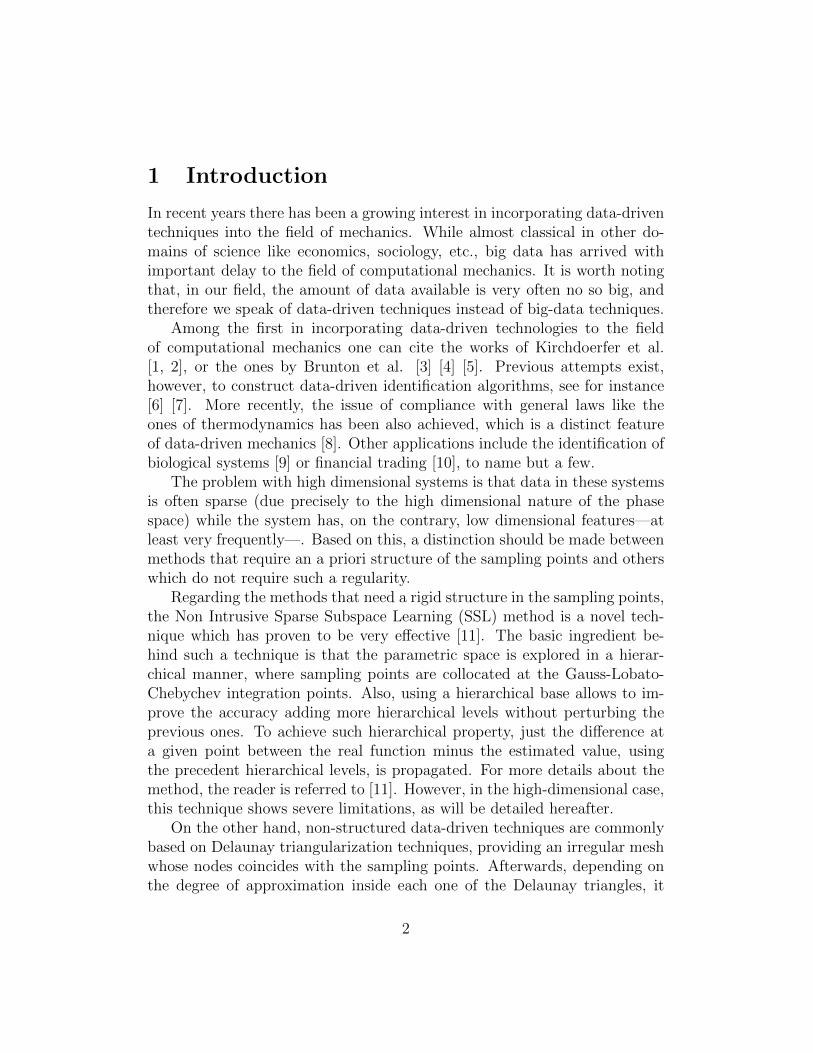
Figs. 1-2 depict the appearance of the simple Kriging interpolants using 7control points uniformly distributed along the domain, for h = 1 and h = 1

3,

respectively. It can be highlighted that both the Kronecker delta (i.e., strictinterpolation) and partition of unity properties are satisfied for any valueof h. Moreover, it is worth noting that the higher the variance the corre-lation function has, the more global the shape functions are. Furthermore,it is known that 99 per cent of the probability of a Gaussian distribution iscomprised within a interval of [m − 3σ,m + 3σ], being m the mean valueof the distribution. This issue explains perfectly well why the support ofeach Gaussian distribution takes 2 elements for the case where h = 1

3. In-

deed, the shape of the interpolants is quite similar to standard finite elementshape functions, but with a Gaussian profile. The remaining 1 per cent ofprobability is comprised in the small ridges happening in the middle of theelements.

In light of these results, a family of interpolants based on Kriging can beeasily created just selecting the value of the variance within the correlationfunction. Therefore, globality of the support can be easily adjusted alwaysunder the framework of the partition of unity.

2.4 Modal adaptivity strategy

In a standard PGD framework, the final solution is approximated as a sumof M modes or functional products, see Eq. (2). Each one of the separatedmodes must be projected onto a chosen basis to render the problem finitedimensional. A standard choice is to select the same basis for each one ofthe modes:

N1 = N2 = . . . = NM .

11

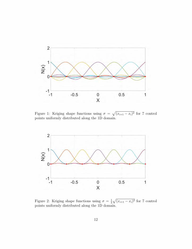
Figure 1: Kriging shape functions using σ =√

(xi+1 − xi)2 for 7 controlpoints uniformly distributed along the 1D domain.

Figure 2: Kriging shape functions using σ = 13

√(xi+1 − xi)2 for 7 control

points uniformly distributed along the 1D domain.

12

Despite of the fact that this choice seems reasonable, when dealing withnon-structured sparse data, it may not be such. In the previous section weproved that the rank of the separated system strongly depends on the distri-bution of the data sampling. Therefore, the cardinality of the interpolationbasis must not exceed the maximum rank provided by the data sampling.Indeed, this constraint, which provides an upper bound to build the interpo-lation basis, only guarantees that the minimization is satisfied at the sam-pling points, without saying anything out of the measured points. Hence, ifsampling points are not abundant, in the limit of low-data regime, high oscil-lations may appear out of these measured points. These oscillations are notdesirable since the resulting prediction properties of the proposed methodcould be potentially decimated.

In order to tackle this problem, we take advantage of the residual-basednature of the PGD. Indeed, the greedy PGD algorithm tries to enrich asolution composed by M modes,

uM(x, y) =M∑k=1

Xk(x)Y k(y),

just by looking at the residual that accounts for the contribution of theprevious modes, as shown in Eq. (8).

Therefore, an appealing strategy to minimize spurious oscillations out ofthe sampling points is to start the PGD algorithm looking for modes withrelatively smooth basis (for instance, Kriging interpolants with a few controlpoints). Therefore, an indicator in order to make an on-line modal adaptivestrategy is required. In the present work, we use the norm of the PGDresidual,

RMP =

1√P

√∑i∈P

(f(xi, yi)− uM(xi, yi))2,

where P is the set of P measured points and f(x, y) is the function to becaptured.

In essence, when the residual norm stagnates, a new control mesh is de-fined, composed by one more control point and always uniformly distributed,following

∆RMP = RM

P −RM−1P < εr.

By doing this, oscillations are reduced, since higher-order basis will try tocapture only what remains in the residual. Here, εr is a tolerance defining the

13

resilience of the sPGD to increase the cardinality of the interpolation basis.The lower εr is, the more resilient the method is to increase the cardinality.

To better understand the method, we will quantify the error for two setof points: the first set is associated to the sampling points, P ,

EP =1

#P∑s∈P

√(f(xs, ys)− uM(xs, ys))2

f(xs, ys)2,

where f(xs, ys) is assumed not to vanish and where L also includes pointsother than the sampling points. This is done in order to validate the algo-rithm, by evaluating the reference solution—which is a priori unknown in ageneral setting—at points different to the sampling ones,

EL =1

#L∑s∈L

√(f(xs, ys)− uM(xs, ys))2

f(xs, ys)2.

Since the s-PGD algorithm minimizes the error only at the samplingpoints P it is reasonable to expect that EP ≤ EL.

2.5 A preliminary example

To test the convergence of the just presented algorithm, we consider

f1(x, y) = (cos(3πx) + sin(3πy))y2 + 4,

that presents a quite oscillating behavior along the x direction, whereas they direction is quadratic. We are interested in capturing such a function inthe domain Ωy = Ωx = [−1, 1].

Figs. (3)-(4) show the errors EP and EL in identifying the function f1(x, y).In this case, we consider two distinct possibilities: no modal adaptivity atall, and a modal adaptivity based on the residual, respectively. Several as-pects can be highlighted. The first one is that EP (asterisks) decreases muchfaster when there is no modal adaptivity. This is expected, since we areminimizing with a richer basis since the very beginning, instead of startingwith smooth functions like in the residual based approach. However, evenif the minimization in the sampling points is well achieved, when no modaladaptivity is considered, the error out of the sampling points may increaseas the solution is enriched with new modes. Nevertheless, the residual-based

14

Figure 3: EL (points) and EP (asterisk) versus the number of modes forf1(x, y), #P = 100, #L = 1000. No modal adaptivity.

modal adaptivity alleviates this problem. As it can be noticed, starting withrelatively smooth functions drives the solution out of the sampling points tobe smooth as well, avoiding the problem of high oscillations appearing outof the sampling points.

3 A local approach to s-PGD

It is well-known that, as in POD, reduced basis or, in general, any otherlinear model reduction technique, PGD gives poor results—in the form ofa non-parsimonious prediction—when the solution of the problem lives in ahighly non-linear manifold. Previous approaches to this difficulty includedthe employ of non-linear dimensionality reduction techniques such as LocallyLinear Embeddings [22], kernel Principal Component Analysis [23] [24] orisomap techniques [25]. Another, distinct, possibility, is to employ a localversion of PGD [18], in which the domain is sliced so that at every sub-regionPGD provides optimal or nearly optimal results. We explore this last optionhere for the purpose of sparse regression, although a bit modified, as will bedetailed hereafter.

The approach followed herein is based on the employ of the partition ofunity property [26] [27]. In essence, it is well-known that any approximat-

15

Figure 4: EL (points) and EP (asterisk) versus the number of modes forf1(x, y), #P = 100, #L = 1000. Modal adaptivity based on the residual,εr=1e-2.

ing function (like finite element shape functions, for instance) that forms apartition of unity can be enriched with an arbitrary function such that theresulting approximation inherits the smoothness of the partition of unity andthe approximation properties of the enriching function.

With this philosophy in mind, we proposed to enrich a finite elementmesh with an s-PGD approximation. The resulting approximation will belocal, due to the compact support of finite element approximation, whileinheriting the good approximation properties, already demonstrated, of s-PGD. In essence, what we propose is to construct an approximation of thetype

u(x, y) ≈∑i∈I

Ni(x, y)ui +∑

p∈Ienr

∑e∈Ip

Ne(x, y)M∑k=1

Xkp (x)Y k

p (y)︸ ︷︷ ︸fenrp (x,y)

,

where I represents the node set in the finite element mesh, Ienr the setof enriched nodes, ui are the nodal degrees of freedom of the mesh, Ip isthe number of finite elements covered by node p shape function’s supportand Xk

p (x) and Y kp (x) functions are the k-th one-dimensional PGD modes

enriching node p, that in fact constitute an enriching function f enr(x, y).

16

Of course, as already introduced in Eqs. (4) and (5), every PGD mode isin turn approximated by Galerkin projection on a judiciously chosen basis.In other words,

u(x, y) ≈∑i∈I

Ni(x, y)ui +∑

p∈Ienr

∑e∈Ip

Ne(x, y)M∑k=1

(Nkx)Tak

p(Nky)Tbk

p, (9)

with akp and bk

p the nodal values describing each one-dimensional PGD mode.In this framework, the definition of a suitable test function can be done

in several ways. As a matter of fact, the test function can be expressed asthe sum of a finite element and a PGD contribution,

u∗ = u∗FEM + u∗PGD,

so that an approach similar to that of Eq. (3) can be accomplished.An example of the performance of this approach is included in Section

4.4.

4 Numerical results

The aim of this section is to compare the ability of sparse model identifica-tion for different interpolation techniques. On one hand, the performance ofstandard techniques based on Delaunay triangulation such as linear, nearestneighbor or cubic interpolation is compared. Even though these techniquesare simple, they allow to have a non-structured sampling point set since theyrely on a Delaunay triangulation. On the other hand, the results are com-pared to the Sparse Subspace Learning (SSL) [11]. The convergence androbustness of this method is proven to be very effective since the points arecollocated at the Gauss-Lobato-Chebychev points. However, two main draw-backs appear considering this method. The first one is that there is a highconcentration of points in the boundary of the domain, so that this quadra-ture is meant for functions that vary mainly along the boundary. Indeed,if the variation of the function appears in the middle of the domain, manysampling points will be required to converge to the exact function. The sec-ond one is that the sampling points have to be located at specific points inthe domain. The s-PGD method using simple Kriging interpolants will becompared as well.

17

Figure 5: EL of f1(x, y) varying #P for different identification techniques.#L = 1000.

The numerical results are structured as follows: first two synthetic 2Dfunctions are analyzed; secondly, two 2D response surfaces coming from athermal problem and a Plastic Yield function are reconstructed; finally, a10D synthetic function is reconstructed by means of the s-PGD algorithm.

4.1 2D synthetic functions

The first considered function is f1(x, y), as introduced in the previous section.Fig. 5 shows the reconstruction error (EL) of f1(x, y) for different samplingpoints. As it can be noticed, the s-PGD algorithm performs well for a widerange of sampling points. Nevertheless, the SSL method is the one presentingthe lower error level when there are more than 150 sampling points.

A second synthetic function is defined as

f2(x, y) = cos(3xy) + log(x+ y + 2.05) + 5.

This function is intended to be reconstructed in the domain Ωx = Ωy =[−1, 1]. It was chosen in such a way that it is relatively smooth in the centerof the domain, whereas the main variation is located along the boundary ofthe domain. Indeed, this function is meant to show the potential of the SSLtechnique.

18

Figure 6: EL of f2(x, y) varying #P for different identification techniques.#L = 1000.

Fig. 6 shows the reconstruction error of the f2(x, y) function for differentinterpolation techniques. As it can be noticed, both SSL and s-PGD methodsare the ones that present the best convergence properties. If the number ofpoints is increased even more, the SSL method is the one that presents thelowest interpolation error. They are followed by linear and natural neighborinterpolations. Finally, the nearest neighbor method is the one presentingthe worst error for this particular case.

4.2 2D response surfaces coming from physical prob-lems

Once the convergence of the methods have been unveiled for synthetic func-tions, it is very interesting to analyze the power of the former methods bytrying to identify functions that are coming from either simulations or mod-els popular in the computational mechanics community. Indeed, two func-tions will be analyzed: the first one is an anisotropic Plastic Yield function,whereas the second one is a solution coming from a quasi-static thermalproblem with varying source term and conductivity.

Fig. 7 shows the Yld2004-18p anisotropic plastic yield function, defined

19

by Barlat et al. in [28]. Under plane stress hypothesis, this plastic yieldfunction is a convex and closed surface defined in a three-dimensional space.Therefore, the position vector of an arbitrary point in the surface can beeasily parameterized in cylindrical coordinates as R(θ, σxy). The R(θ, σxy)function for the Yld2004-18p is shown in Fig. 8, where anisotropies can beeasily seen. Otherwise, the radius function will be constant for a given σxy.

Figure 7: Barlat’s Yld2004-18p function under plane stress hypothesis.

Fig. 9 shows the error in the identification of the Barlat’s plastic yieldfunction Yld2004-18p. As it can be noticed, the s-PGD technique outper-forms the rest of techniques. Indeed, the s-PGD is exploiting the fact thatthe response surface is highly separable.

As mentioned above, the second problem is the sparse identification ofthe solution of a quasi-static thermal problem modeled by

∇ · (η(x, t)∇(u(x, t))) = f(t), in Ωx × Ωt = [−1, 1]× [−1, 1], (10)

20

Figure 8: R(θ, σxy) function for Barlat’s Yld2004-18p yield function.

Figure 9: EL of R(θ, σxy) varying #P for different sparse identification tech-niques. #L = 1000. εr = 5 · 10−4.

21

Figure 10: Quasi-static solution to the thermal problem u(x, t).

where conductivity varies in space-time as

η(x, t) = (1 + 10 abs(x) + 10x2) log(t+ 2.5) u(1, t) = 2 (11)

f(x, t) = 10 cos(3πt) u(−1, t) = 2, (12)

and the source term varies in time. Homogeneous Dirichlet boundary con-ditions are imposed at both spatial boundaries and no initial conditions arerequired due to quasi-stationarity assumptions.

Fig. 10 shows the evolution of the temperature field as a function of spacetime for the set of Eqs. (10)-(12). It can be noticed how the variation of thetemperature throughout time is caused mainly due to the source term. How-ever, conductivity modifies locally the curvature of the temperature alongthe spatial axis. Symmetry with respect the x = 0 axis is preserved due tothe fact that the conductivity presents a symmetry along the same axis.

Fig. 11 shows the performance of each one of the techniques when tryingto reconstruct the temperature field from certain sampling points. As canbe noticed, the s-PGD in conjunction with Kriging interpolants is the onethat presents the fastest convergence rate to the actual function, which isconsidered unknown. It is followed by linear and natural interpolations. TheSSL method presents a slow convergence rate in this case, due to the factthat the main variation of the function u(x, t) is happening in the center of

22

Figure 11: EL of u(x, t) varying #P for different identification techniques.#L = 1000. εr = 2.5 · 10−3.

the domain and not in the boundary.

4.3 A 10D multivariate case

In this subsection, we would like to show the scalability that s-PGD presentswhen dealing with relatively high-dimensional spaces. Since our solution isexpressed in a separated format, an N dimensional problem (ND) is solved asa sequence of N 1D problems, which are solved using a fixed-point algorithmin order to circumvent the non-linearity of the separation of variables.

The objective function that we have used to analyze the properties of thes-PGD is defined as

f3(x1, x2, . . . , xN) = 2 +1

8

N∑i=1

xi +N∏i=1

xi +N∏i=1

x2i ,

with N = 10 in this case.Fig. 12 shows the error convergence in both sampling points (EP , aster-

isks) and points out of the sampling (EL, filled points). The L data set wascomposed by 3000 points, the P data subset for the s-PGD algorithm wascomposed by 500 points. The number of points required to properly capture

23

Figure 12: EL (points) and EP (asterisk) versus the number of modes forf3(x1, x2, . . . , xN), #P = 500, #L = 3000. Modal adaptivity based on theresidual, εr = 1e− 3.

the hyper-surface has increased with respect to the 2D examples due to thehigh dimensionality of the problem. Special attention has to be paid whenincreasing the cardinality of the interpolant basis without many samplingpoints, because the problem of high oscillations outside the control pointsmay be accentuated.

4.4 An example of the performance of the local s-PGD

The last example corresponds to the sparse regression of an intricate surface,that has been created by mixing three different Gaussian surfaces so as togenerate a surface with no easy separate representation (a non parsimoniousmodel, if we employ a different vocabulary). The appearance of this syntheticsurface is shown in Fig. 13.

The sought surface is defined in the domain Ω = [0, 1]2, which has beensplit into the finite element mesh shown in Fig. 14. Every element in themesh has been colored according to the number of enriching PGD functions,ranging from a single one to four. The convergence plot of this example as afunction of the number of PGD modes added to the approximating space isincluded in Fig. 15.

24

Figure 13: A synthetic surface generated by superposition of three differentGaussians, that is to be approximated by local s-PGD techniques.

Figure 14: Finite element mesh for the example in Section 4.4. All theinternal nodes have been enriched.

25

Figure 15: Convergence plot for the example in Section 4.4.

5 Conclusions

In this paper we have developed a data-based sparse reduced-order regres-sion technique under the Proper Generalized Decomposition framework. Thisalgorithm combines the robustness typical of the separation of variables to-gether with properties of collocation methods in order to provide with par-simonious models for the data at hand. The performance of simple Kriginginterpolation has proven to be effective when the sought model presents someregularity. Furthermore, a modal adaptivity technique has been proposed inorder to avoid high oscillations out of the sampling points, characteristic ofhigh order interpolation methods when data is sparse.

For problems in which the result lives in a highly non-linear manifold, alocal version of the technique, that makes use of the partition of unity prop-erty, has also been developed. This local version outperforms the standardone for very intricate responses.

The s-PGD method has been compared advantageously versus other ex-isting methods for different example functions. Finally, the convergence ofs-PGD method for a high dimensional function has been demonstrated aswell.

Although the sparsity of the obtained solution could not seem evident

26

for the reader, we must highlight the fact that the very nature of the PGDstrategy a priori selects those terms in the basis that play a relevant rolein the approximation. So to speak, PGD algorithms automatically discardthose terms that in other circumstances will be weighted by zero. Sparsity,in this sense, is equivalent in this context to the number of sums in the PGDseparated approximation. If only a few terms are enough to reconstruct thedata—as is almost always the case—, then sparsity is guaranteed in practice.

Sampling strategies other than the latin hypercube method could be ex-amined as well. This, and the coupling with error indicators to establishgood stopping criteria, constitute our effort of research at this moment. Infact, the use of reliable error estimators could even allow for the obtentionof adaptive samplings in which the cardinality of the basis could be differentalong different directions.

Acknowledgements

This project has received funding from the European Union’s Horizon 2020research and innovation program under the Marie Sklodowska-Curie grantagreement No. 675919. Also by the Spanish Ministry of Economy and Com-petitiveness through Grants number DPI2017-85139-C2-1-R and DPI2015-72365-EXP and by the Regional Government of Aragon and the EuropeanSocial Fund, research group T24 17R.

References

[1] T. Kirchdoerfer and M. Ortiz. Data-driven computational mechanics.Computer Methods in Applied Mechanics and Engineering, 304:81 – 101,2016.

[2] T. Kirchdoerfer and M. Ortiz. Data driven computing with noisy mate-rial data sets. Computer Methods in Applied Mechanics and Engineering,326:622 – 641, 2017.

[3] Steven L. Brunton, Joshua L. Proctor, and J. Nathan Kutz. Discov-ering governing equations from data by sparse identification of non-linear dynamical systems. PROCEEDINGS OF THE NATIONAL

27

ACADEMY OF SCIENCES OF THE UNITED STATES OF AMER-ICA, 113(15):3932–3937, APR 12 2016.

[4] Steven L Brunton, Joshua L Proctor, and J Nathan Kutz. Sparse iden-tification of nonlinear dynamics with control (sindyc). arXiv preprintarXiv:1605.06682, 2016.

[5] Markus Quade, Markus Abel, J. Nathan Kutz, and Steven L. Brunton.Sparse identification of nonlinear dynamics for rapid model recovery.Chaos: An Interdisciplinary Journal of Nonlinear Science, 28(6):063116,2018.

[6] D. Gonzalez, F. Masson, F. Poulhaon, E. Cueto, and F. Chinesta. Propergeneralized decomposition based dynamic data driven inverse identifica-tion. Mathematics and Computers in Simulation, 82:1677–1695, 2012.

[7] Benjamin Peherstorfer and Karen Willcox. Data-driven operator in-ference for nonintrusive projection-based model reduction. ComputerMethods in Applied Mechanics and Engineering, 306:196 – 215, 2016.

[8] David Gonzalez, Francisco Chinesta, and Elıas Cueto. Thermodynami-cally consistent data-driven computational mechanics. Continuum Me-chanics and Thermodynamics, May 2018.

[9] N. M. Mangan, S. L. Brunton, J. L. Proctor, and J. N. Kutz. Inferringbiological networks by sparse identification of nonlinear dynamics. IEEETransactions on Molecular, Biological and Multi-Scale Communications,2(1):52–63, June 2016.

[10] Jordan Mann and J. Nathan Kutz. Dynamic mode decomposition forfinancial trading strategies. Quantitative Finance, 16(11):1643–1655,2016.

[11] Domenico Borzacchiello, Jose V. Aguado, and Francisco Chinesta. Non-intrusive sparse subspace learning for parametrized problems. Archivesof Computational Methods in Engineering, Jul 2017.

[12] Charles Epstein, Gunnar Carlsson, and Herbert Edelsbrunner. Topolog-ical data analysis. Inverse Problems, 27(12):120201, 2011.

28

[13] W. Guo, K. Manohar, S. L. Brunton, and A. G. Banerjee. Sparse-tda: Sparse realization of topological data analysis for multi-way clas-sification. IEEE Transactions on Knowledge and Data Engineering,30(7):1403–1408, July 2018.

[14] F. Chinesta, A. Ammar, and E. Cueto. Recent advances in the useof the Proper Generalized Decomposition for solving multidimensionalmodels. Archives of Computational Methods in Engineering, 17(4):327–350, 2010.

[15] Francisco Chinesta, Roland Keunings, and Adrien Leygue. TheProper Generalized Decomposition for Advanced Numerical Simulations.Springer International Publishing Switzerland, 2014.

[16] F. Chinesta and P. Ladeveze, editors. Separated Representations andPGD-Based Model Reduction. Springer International Publishing, 2014.

[17] D. Gonzalez, A. Ammar, F. Chinesta, and E. Cueto. Recent advanceson the use of separated representations. International Journal for Nu-merical Methods in Engineering, 81(5), 2010.

[18] Alberto Badıas, David Gonzalez, Iciar Alfaro, Francisco Chinesta,and Elias Cueto. Local proper generalized decomposition. Interna-tional Journal for Numerical Methods in Engineering, 112(12):1715–1732, 2017. nme.5578.

[19] E. Cueto, D. Gonzalez, and I. Alfaro. Proper Generalized Decom-positions: An Introduction to Computer Implementation with Matlab.SpringerBriefs in Applied Sciences and Technology. Springer Interna-tional Publishing, 2016.

[20] David Gonzalez, Alberto Badıas, Icıar Alfaro, Francisco Chinesta, andElıas Cueto. Model order reduction for real-time data assimilationthrough Extended Kalman Filters. Computer Methods in Applied Me-chanics and Engineering, 326(Supplement C):679 – 693, 2017.

[21] Jean-Christophe Loiseau and Steven L. Brunton. Constrained sparsegalerkin regression. Journal of Fluid Mechanics, 838:42–67, 2018.

[22] Sam T. Roweis and Lawrence K. Saul. Nonlinear dimensionality reduc-tion by locally linear embedding. Science, 290(5500):2323–2326, 2000.

29

[23] Bernhard Scholkopf, Alexander Smola, and Klaus-Robert Muller. Non-linear component analysis as a kernel eigenvalue problem. Neural Com-put., 10(5):1299–1319, July 1998.

[24] B. Scholkopf, A. Smola, and K.R. Muller. Kernel principal componentanalysis. In ADVANCES IN KERNEL METHODS - SUPPORT VEC-TOR LEARNING, pages 327–352. MIT Press, 1999.

[25] Joshua B. Tenenbaum, Vin de Silva, and John C. Langford. A globalgeometric framework for nonlinear dimensionality reduction. Science,290(5500):2319–2323, 2000.

[26] I. Babuska and J. M. Melenk. The partition of unity finite elementmethod: Basic theory and applications. Comp. Meth. in Appl. Mech.and Eng., 4:289–314, 1996.

[27] I. Babuska and J. M. Melenk. The partition of unity method. Interna-tional Journal for Numerical Methods in Engineering, 40:727–758, 1997.

[28] J.W. Yoon, F. Barlat, R.E. Dick, and M.E. Karabin. Prediction of sixor eight ears in a drawn cup based on a new anisotropic yield function.International Journal of Plasticity, 22(1):174 – 193, 2006.

30