A Multi-Task Learning Formulation for PredictingDisease Progression

Jiayu Zhou, Lei Yuan, Jun Liu, Jieping YeComputer Science and Engineering, Center for Evolutionary Medicine and Informatics, The Biodesign

Institute, Arizona State University, Tempe, AZ 85287{Jiayu.Zhou, Lei.Yuan, Jun.Liu, Jieping.Ye}@asu.edu

ABSTRACTAlzheimer’s Disease (AD), the most common type of de-mentia, is a severe neurodegenerative disorder. Identifyingmarkers that can track the progress of the disease has re-cently received increasing attentions in AD research. Adefinitive diagnosis of AD requires autopsy confirmation,thus many clinical/cognitive measures including Mini Men-tal State Examination (MMSE) and Alzheimer’s Disease As-sessment Scale cognitive subscale (ADAS-Cog) have beendesigned to evaluate the cognitive status of the patients andused as important criteria for clinical diagnosis of probableAD. In this paper, we propose a multi-task learning formu-lation for predicting the disease progression measured by thecognitive scores and selecting markers predictive of the pro-gression. Specifically, we formulate the prediction problemas a multi-task regression problem by considering the pre-diction at each time point as a task. We capture the intrinsicrelatedness among different tasks by a temporal group Lassoregularizer. The regularizer consists of two components in-cluding an ℓ2,1-norm penalty on the regression weight vec-tors, which ensures that a small subset of features will beselected for the regression models at all time points, and atemporal smoothness term which ensures a small deviationbetween two regression models at successive time points.We have performed extensive evaluations using various typesof data at the baseline from the Alzheimer’s Disease Neu-roimaging Initiative (ADNI) database for predicting the fu-ture MMSE and ADAS-Cog scores. Our experimental stud-ies demonstrate the effectiveness of the proposed algorithmfor capturing the progression trend and the cross-sectionalgroup differences of AD severity. Results also show thatmost markers selected by the proposed algorithm are con-sistent with findings from existing cross-sectional studies.

Categories and Subject DescriptorsH.2.8 [Database Management]: Database Applications—Data Mining ; J.3 [Life and Medical Sciences]: Health,Medical information systems

Permission to make digital or hard copies of all or part of this work forpersonal or classroom use is granted without fee provided that copies arenot made or distributed for profit or commercial advantage and that copiesbear this notice and the full citation on the first page. To copy otherwise, torepublish, to post on servers or to redistribute to lists, requires prior specificpermission and/or a fee.KDD’11, August 21–24, 2011, San Diego, California, USA.Copyright 2011 ACM 978-1-4503-0813-7/11/08 ...$10.00.

General TermsAlgorithms

KeywordsAlzheimer’s Disease, regression, multi-task learning, groupLasso, stability selection, cognitive score

1. INTRODUCTIONAlzheimer’s disease (AD), the most common type of de-

mentia, is characterized by the progressive impairment ofneurons and their connections resulting in loss of cognitivefunction and ultimately death [20]. AD currently affectsabout 5.3 million individuals in United States and more than30 million worldwide with a significant increase predicted inthe near future [5]. Alzheimer’s disease has been not onlythe substantial financial burden to the health care systembut also the psychological and emotional burden to patientsand their families. As the research on developing promisingnew treatments to slow or prevent AD progressing, the needfor markers that can track the progress of the disease andidentify it early becomes increasingly urgent.

A definitive diagnosis of AD can only be made throughan analysis of brain tissue during a brain biopsy or au-topsy [18]. Many clinical/cognitive measures have been de-signed to evaluate the cognitive status of the patients andused as important criteria for clinical diagnosis of proba-ble AD, such as Mini Mental State Examination (MMSE)and Alzheimer’s Disease Assessment Scale cognitive subscale(ADAS-Cog) [25]. MMSE has been shown to be correlatedwith the underlying AD pathology and progressive deterio-ration of functional ability [18]. ADAS-Cog is the gold stan-dard in AD drug trial for cognitive function assessment [31].Since neurodegerenation of AD proceeds years before the on-set of the disease and the therapeutic intervention is moreeffective in the early stage of the disease, there is thus an ur-gent need to address two major research questions: (1) howcan we predict the progression of the disease measured bycognitive scores, e.g., MMSE and ADAS-Cog? (2) what isthe smallest set of features (measurements) most predictiveof the progression? The prime candidate markers for track-ing disease progression include neuroimages such as mag-netic resonance imaging (MRI), cerebrospinal fluid (CSF),and baseline clinical assessments [12].

The relationship between the cognitive scores and possiblerisk factors such as age, APOE gene, years of education andgender has been previously studied [36, 17]. Many existingworks analyzed the relationship between cognitive scores and

imaging markers based on MRI such as gray matter volumes,density and loss [3, 8, 15, 16, 33], shape of ventricles [14,34] and hippocampal [34] by correlating these features withbaseline MMSE scores. In [13], the intensity and volumeof medial temporal lobe altogether with other risk factorsand the gray matter were shown to be correlated with the 6-month MMSE score, which allowed us to predict near-futureclinical scores of patients. Relations between 6-month atro-phy patterns in medial temporal region and memory dec-lination in terms of clinical scores had also been examinedin [27]. To predict the longitudinal response to Alzheimer’sDisease progression, Ashford and Schmitt built a model withhorologic function using “time-index” to measure the rate ofdementia progression [4]. In [10], the so-called SPARE-ADindex was proposed based on spatial patterns of brain at-rophy and its linear effect against MMSE was reported. Ina more recent study by Ito et al., the progression rate ofcognitive scores was modeled using power functions [17].Most existing work employed either the regression model

[13, 33] or the survival model [37] for modeling the diseaseprogression. The correlation between the ground truth andthe prediction is used to evaluate the model [13, 33]. Whenthe size of covariates is small, each covariate can be indi-vidually added to the model to examine its effectiveness forpredicting the target [17, 38], or univariate analysis is per-formed individually on all covariates and those who exceed acertain significance threshold are included in the model [27].When the number of covariates is large and significant corre-lations among covariates exist, these approaches are subop-timal. To deal with the curse of dimensionality, dimensionreduction techniques are commonly employed. Duchesne etal. used principle components analysis (PCA) to build a lowdimensional feature space from image data [13]. An obvi-ous disadvantage of dimension reduction techniques such asPCA is that the model is no longer interpretable, since allfeatures are involved. Stonnington et al. used relevance vec-tor regression (RVR), which integrated feature selection inthe training stage [33]. These approaches only predict clini-cal scores at a single time point and their performances arefar from satisfactory to be clinically useful for AD prognosis.In this paper, we propose a multi-task learning formula-

tion for predicting the progression of the disease measuredby the clinical scores at multiple time points and simultane-ously selecting markers predictive of the progression. Specif-ically, we formulate the prediction of clinical scores at a se-quence of time points as a multi-task regression problem,where each task concerns the prediction of a clinical scoreat one time point. Multi-task learning aims at improvingthe generalization performance by learning multiple relatedtasks simultaneously. The key of multi-task learning is toexploit the intrinsic relatedness among the tasks. For thedisease progression considered in this paper, it is reasonableto assume that a small subset of features is predictive of theprogression, and the multiple regression models from dif-ferent time points satisfy the smoothness property, that is,the difference of the cognitive scores between two successivetime points is small. To this end, we develop a novel multi-task learning formulation based on a temporal group Lassoregularizer. The regularizer consists of two components in-cluding an ℓ2,1-norm penalty [39] on the regression weightvectors, which ensures that a small subset of features will beselected for the regression models at all time points, and a

temporal smoothness term, which ensures a small deviationbetween two regression models at successive time points.

We have performed extensive experimental studies to eval-uate the effectiveness of the proposed algorithm. We usevarious types of data from the Alzheimer’s Disease Neu-roimaging Initiative (ADNI) database including MRI scans,CSF, and clinical scores at the baseline to predict the MMSEand ADAS-Cog scores for the next three years. Our ex-perimental studies show that the proposed algorithm bet-ter captures the progression trend and the cross-sectionalgroup differences of AD severity than existing methods. Re-sults also show that most markers selected by the proposedalgorithm are consistent with findings from existing cross-sectional studies.

2. PROPOSED MULTI-TASK REGRESSIONFORMULATION

In the longitudinal AD study, we measure the cognitivescores of selected patients repeatedly at multiple time points.By considering the prediction of cognitive scores at a singletime point as a regression task, we formulate the progressionof clinical scores as a multi-task regression problem. We em-ploy the multi-task regression formulation instead of solvinga set of independent regression problems since the intrinsictemporal smoothness information among different tasks canbe incorporated into the model as prior knowledge.

Consider a multi-task regression problem of t time pointswith n training samples of d features. Let {x1, x2, · · · , xn}be the input data at the baseline, and {y1, y2, · · · , yn} be thetargets, where each xi ∈ Rd represents a sample (patient),and yi ∈ Rt is the corresponding targets (clinical scores)at different time points. In this paper we employ linearmodels for the prediction. Specifically, the prediction modelfor the ith time point is given by f i(x) = xTwi, where wi

is the weight vector of the model. Let X = [x1, · · · , xn]T ∈

Rn×d be the data matrix, Y = [y1, · · · , yn]T ∈ Rn×t bethe target matrix, and W =

[w1, w2, ..., wt

]∈ Rd×t be the

weight matrix. One simple approach is to estimate W byminimizing the following objective function:

minW

∥XW − Y ∥2F + θ1 ∥W∥2F , (1)

where the first term measures the empirical error on thetraining data, the second (penalty) term controls the gen-eralization error, θ1 > 0 is a regularization parameter, and∥.∥F is the Frobenius norm of a matrix. The regressionmethod above is known as the ridge regression and it ad-mits an analytical solution given by:

W = (XTX + θ1I)−1XTY. (2)

One major limitation of the regression model above is thatthe tasks at different time points are assumed to be inde-pendent with each other, which is not the case in the longi-tudinal AD study considered in this paper.

2.1 Temporal Smoothness PriorTo capture the temporal smoothness of the cognitive scores

at different time points, we introduce a regularization termin the regression model that penalizes large deviations ofpredictions at neighboring time points, resulting in the fol-

lowing formulation:

minW

∥XW − Y ∥2F + θ1 ∥W∥2F + θ2

t−1∑i=1

∥∥∥wi − wi+1∥∥∥2

2, (3)

where θ2 ≥ 0 is a regularization parameter controlling thetemporal smoothness. This temporal smoothness term canbe expressed as:

t−1∑i=1

∥∥∥wi − wi+1∥∥∥2

F= ∥WH∥2F ,

where H ∈ Rt×(t−1) is defined as follows: Hij = 1 if i =j, Hij = −1 if i = j + 1, and Hij = 0 otherwise. Theformulation in Eq.(3) becomes:

minW

∥XW − Y ∥2F + θ1 ∥W∥2F + θ2 ∥WH∥2F . (4)

The optimization problem in Eq.(4) admits an analyticalsolution, as shown below. First, we take the derivative ofEq.(4) with respect to W and set it to zero:

XTXW −XTY + θ1W + θ2WHHT = 0, (5)(XTX + θ1Id

)W +W

(θ2HHT

)= XTY, (6)

where Id is the identity matrix of size d by d. Since both ma-trices (XTX+θ1Id) and θ2HHT are symmetric, we write theeigen-decomposition of these two matrices by Q1Λ1Q

T1 and

Q2Λ2QT2 , where Λ1 = diag(λ

(1)1 , λ

(2)1 , . . . , λ

(d)1 ) and Λ2 =

diag(λ(1)2 , λ

(2)2 , . . . , λ

(d)2 ), are their eigenvalues, and Q1 and

Q2 are orthogonal. Plugging them into Eq. (6) we get:

Q1Λ1QT1 W +WQ2Λ2Q

T2 = XTY, (7)

Λ1QT1 WQ2 +QT

1 WQ2Λ2 = QT1 X

TY Q2. (8)

Denote W = QT1 WQ2 and D = QT

1 XTY Q2. Eq.(8) be-

comes Λ1W + WΛ2 = D. Thus W is given by:

Wi,j =Di,j

λ(i)1 + λ

(j)2

. (9)

The optimal weight matrix is then given by W ∗ = Q1WQT2 .

2.2 Dealing with Incomplete DataThe clinical scores for many patients are missing at some

time points, i.e., the target vector yi ∈ Rt may not be com-plete. A simple strategy is to remove all patients with miss-ing target values, which, however, significantly reduces thenumber of samples. We consider to extend the formulationin Eq.(4) with missing target values in the training process.In this case, the analytical solution to Eq.(4) no longer ex-ists. We show how the algorithm above can be adapted todeal with missing target values.We use a matrix S ∈ Rn×t to indicate missing target

values, where Si,j = 0 if the target value of sample i ismissing at the jth time point, and Si,j = 1 otherwise. Weuse the componentwise operator ⊙ as follows: Z = A ⊙ Bdenotes zi,j = ai,jbi,j , for all i, j. The formulation in Eq.(4)can be extended to the case with missing target values as:

minW

∥S ⊙ (XW − Y )∥2F + θ1 ∥W∥2F + θ2 ∥WH∥2F . (10)

Denote Pr(.) as the row selection operator parameterized bya selection vector r. The resulting matrix of Pr(A) includesonly Ai such that ri = 0, where Ai is the ith row of A.

Let Si be the ith column of S. We therefore denote X(i) =

PSi(X) ∈ Rni×d as the input data matrix of the ith task,and y(i) = PSi(Y i) ∈ Rni×1 as the corresponding targetvector, where ni is number of samples from the ith task.

Similar to the case without missing target values consid-ered in Section 2.1, we take the derivative of Eq.(10) withrespect to wi (2 ≤ i ≤ t− 1) and set it to zero:

Awi−1 +Miwi +Awi+1 = Ti, (11)

where A, Mi, and Ti are defined as follows:

A = −θ2Id,

Mi = XT(i)X(i) + θ1Id + 2θ2Id,

Ti = XT(i)y(i).

For the special case i = 1, the term∥∥wi−1 − wi

∥∥2

2does not

exist, nor is the term∥∥wi − wi+1

∥∥2

2for i = t. We com-

bine the equations for all tasks (1 ≤ i ≤ t), which can berepresented as a block tridiagonal linear system:

M1 A 0A M2 A

. . .

A Mt−1 A0 A Mt

w1

w2

...wt−1

wt

=

T1

T2

...Tt−1

Tt

(12)

For a general linear system of size td, it can be solved usingGaussian elimination with a time complexity of O((td)3).For our block tridiagonal system, the complexity is reducedto O(d3t) using block Gaussian elimination. For large-scalelinear systems, the LSQR algorithm [30], a popular iterativemethod for the solution of large linear systems of equations,can be employed with a time complexity of O(Ntd2), whereN , the number of iterations, is typically small.

2.3 Temporal Group Lasso RegularizationBecause of the limited availability of subjects in the longi-

tudinal AD study and a relatively large number of featuresat ADNI including MRI features, the prediction model suf-fers from the so called“curse of dimensionality”. In addition,many patients drop out from the longitudinal study after acertain period of time, which reduces the effective number ofsamples. One effective approach is to reduce the dimension-ality of the data. However, traditional dimension reductiontechniques such as PCA are not desirable since the resultingmodel is not interpretable, and traditional feature selectionalgorithms are not suitable for multi-task regression withmissing target values. In the proposed formulation, we em-ploy the group Lasso regularization based on the ℓ2,1-normpenalty for feature selection [39], which assumes that a smallset of features are predictive of the progression. The groupLasso regularization ensures that all regression models atdifferent time points share a common set of features. To-gether with the temporal smoothness penalty, we obtain thefollowing formulation:

minW

∥S⊙(XW − Y )∥2F+θ1∥W∥2F+θ2∥WH∥2F+δ∥W∥2,1 (13)

where ∥W∥2,1 =∑d

i=1

√∑tj=1 W

2ij , and δ is a regularization

parameter. When there is only one task, i.e., t = 1, theabove formulation reduces to Lasso [35]. When t > 1, theweights of one feature over all tasks are grouped using the

ℓ2-norm, and all features are further grouped using the ℓ1-norm. Thus, the ℓ2,1-norm penalty tends to select featuresbased on the strength of the feature over all t tasks.The objective in Eq.(13) can be considered as a combina-

tion of a smooth term and a non-smooth term. The gradientdescent or accelerated gradient method (AGM) [29, 28] canbe applied to solve the optimization. One of the key stepsin AGM is the computation of the proximal operator as-sociated with the ℓ2,1-norm regularization. We employ thealgorithm in the SLEP package [22], which computes theproximal operator associated with the general ℓ1/ℓq-normefficiently.

2.3.1 Longitudinal Stability SelectionAn important issue in the practical application of the pro-

posed formulation is the selection of an appropriate amountof regularization, known as model selection. Cross validationis commonly used for model selection, however it tends to se-lect more features than needed [26]. In this paper, we adaptstability selection to perform model selection for the pro-posed multi-task regression. Stability selection is a methodrecently proposed to address the problem of proper regular-ization using subsampling/bootstrapping [26]. It should benoted that in our formulation we find in our experimentsthat the list of top features selected by stability selection isnot sensitive to the regularization parameters θ1 and θ2. Wethus focus on the selection of δ, which controls the sparsityof the model, in stability selection.Let K be the index set of features, i.e., k ∈ K denotes a

feature. Given a set of regularization parameter values ∆and an iteration number γ, longitudinal stability selectionworks as follows. Let B(j) = {BX

(j), BY(j)} be a random sub-

sample from {X,Y } of size ⌊n/2⌋ without replacement. For

a given δ > 0, let W (j) be the optimal solution of Eq.(13) on

B(j). Denote Uδ(B(j)) = {k : W(j)k = 0} as the set of fea-

tures selected by the model W (j). This process is repeatedfor γ times and selection probability Πδ

k of each feature kis given by

∑γj=1 I(k ∈ Uδ(B(j)))/γ, where I(.) is the indi-

cator function defined as follows: I(c) = 1 if c is true and

I(c) = 0 otherwise. It is clear that Πδk computes the fraction

of bootstrap experiments for which the feature k is selected.Repeat the above procedure for all δ ∈ ∆, and we define thestability score for each feature k by S(k) = maxδ∈∆(Πδ

k).

To find a suitable size of stable feature set U stable we caneither use top η stable features:

U stable = {k : S(k) ranks among top η in K},

or use threshold πthr on the stability score:

U stable = {k : S(k) ≥ πthr}.

In our application we choose the top η features. Indeed,cross validation can be performed to determine how manyfeatures are needed. However, our empirical results showthat using top η = 20 features is sufficient in most cases ofour application.

2.4 Proposed AlgorithmOne undesired property of sparse learning methods such

as Lasso is that the coefficients corresponding to relevantfeatures are shrunk towards zero [40]. This shrinkage ef-fect would lead to sub-optimal performance. To resolvethis problem, existing methods apply adaptive regulariza-

tion [42], multiple thresholding procedures [41], or multi-stage methods [23, 40]. In this paper, we employ a standardtwo-stage procedure. In the first stage the algorithm selectsfeatures using longitudinal stability selection, resulting in asubset of features Ustable. In the second stage the algorithmperforms temporal smoothness regularized regression usingselected features. We summarize the proposed algorithm inAlgorithm 1.

Algorithm 1 Temporal Group Lasso Multi-Task Regression(TGL)

Input: S, X, Y, θ1, θ2 ∆, γ, ηOutput: W ∗, U stable

1: Stage 1: longitudinal stability selection2: Set K = {the feature set in X}3: for δ ∈ ∆ do4: for j = 1 to γ do5: Subsample B(j) = {BX

(j), BY(j)} from {X,Y }

6: Compute W (j) by solving Eq.(13) with δ,B(j)

7: Set Uδ(B(j)) = {k : W (j) = 0}8: end for9: Calculate Πδ

k =∑γ

j=1 I(k ∈ Uδ(B(j)))/γ, ∀k ∈ K10: end for11: Calculate S(k) = maxδ∈∆(Πδ

k), ∀k ∈ K

12: Set U stable = {k: S(k) ranks among top η in K}13: Stage 2: temporal smoothness regularized regression14: Set X = X restricted to the features from U stable

15: if ∃p, q such that Sp,q = 0 then

16: Set t = number of tasks, d = |U stable|, A = −θ2Id17: for i = 1 to t do18: X(i) = Pi

S(X), y(i) = PiS(Y

i)

19: Mi = XT(i)X(i) + θ1Id + 2θ2Id, Ti = XT

(i)y(i)20: end for21: Obtain W ∗ by solving Eq.(12) with {Mi}, {Ti}.22: else23: Compute the analytical solution W ∗ as in Section 2.1.24: end if

3. EXPERIMENTSIn this section we evaluate the proposed algorithm on the

ADNI database1. The source codes are available online [1].

3.1 Experimental SetupIn the ADNI project, MRI scans, CSF measurements, and

clinical scores from selected patients are obtained repeatedlyover a 6-month or 1-year interval. We denote each timepoint by the duration starting from the baseline when thepatient came to the hospital for screening. For instance,M06 indicates 6 months after the baseline. We use differentcombinations of MRI (M), CSF (C), and META (M) (seeTable 1) at baseline to predict MMSE and ADAS-Cog scoresat four time points: M06, M12, M24, and M36.

For MRI, we download 1.5T MRI data of 675 patients pre-processed by UCSF using FreeSurfer. MRI features can begrouped into 5 categories: cortical thickness average (CTA),cortical thickness standard deviation (CTStd), volume ofcortical parcellation (Vol. Cort.), volume of white mat-ter parcellation (Vol. WM.), and surface area (Surf. A.).There are 313 MRI features in total. We remove all sam-ples which fail the MRI quality controls. For other feature

1www.loni.ucla.edu/ADNI/

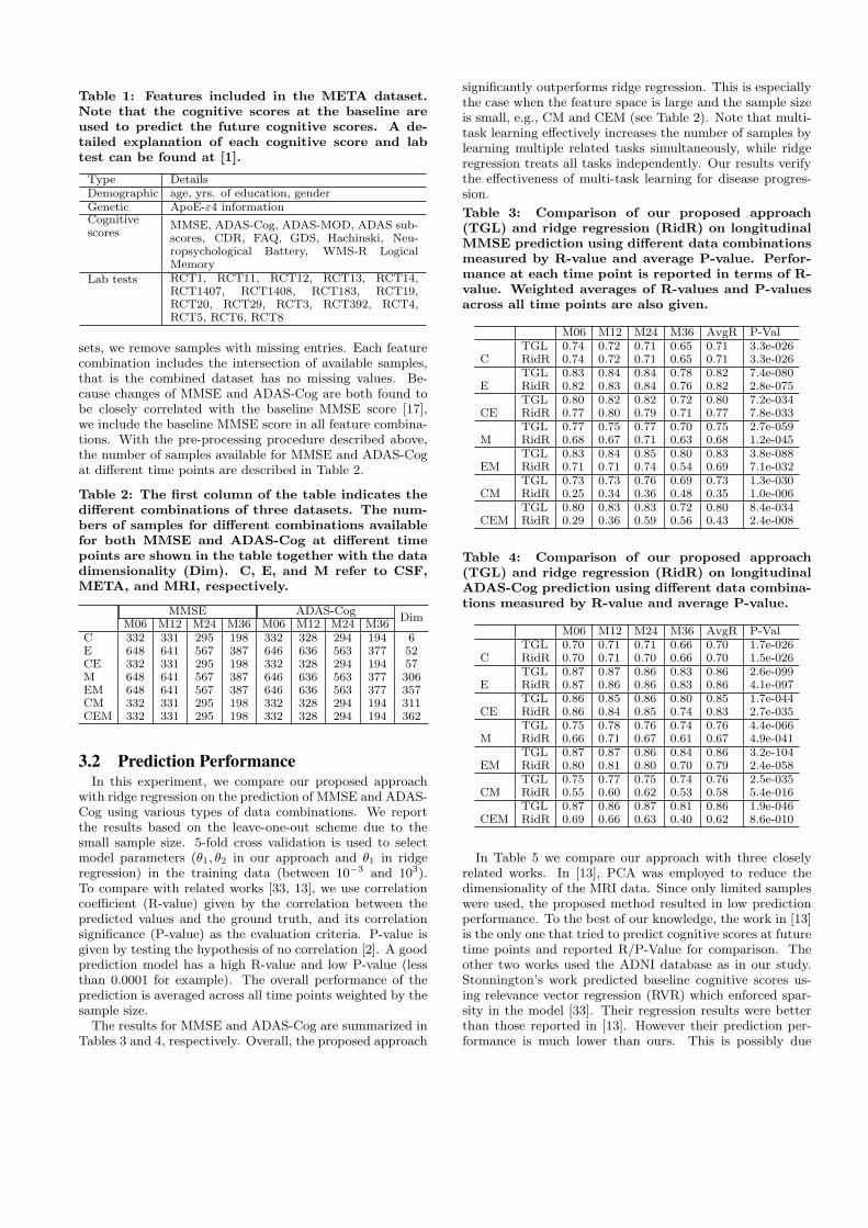
Table 1: Features included in the META dataset.Note that the cognitive scores at the baseline areused to predict the future cognitive scores. A de-tailed explanation of each cognitive score and labtest can be found at [1].

Type DetailsDemographic age, yrs. of education, genderGenetic ApoE-ε4 informationCognitivescores

MMSE, ADAS-Cog, ADAS-MOD, ADAS sub-scores, CDR, FAQ, GDS, Hachinski, Neu-ropsychological Battery, WMS-R LogicalMemory

Lab tests RCT1, RCT11, RCT12, RCT13, RCT14,RCT1407, RCT1408, RCT183, RCT19,RCT20, RCT29, RCT3, RCT392, RCT4,RCT5, RCT6, RCT8

sets, we remove samples with missing entries. Each featurecombination includes the intersection of available samples,that is the combined dataset has no missing values. Be-cause changes of MMSE and ADAS-Cog are both found tobe closely correlated with the baseline MMSE score [17],we include the baseline MMSE score in all feature combina-tions. With the pre-processing procedure described above,the number of samples available for MMSE and ADAS-Cogat different time points are described in Table 2.

Table 2: The first column of the table indicates thedifferent combinations of three datasets. The num-bers of samples for different combinations availablefor both MMSE and ADAS-Cog at different timepoints are shown in the table together with the datadimensionality (Dim). C, E, and M refer to CSF,META, and MRI, respectively.

MMSE ADAS-CogDim

M06 M12 M24 M36 M06 M12 M24 M36C 332 331 295 198 332 328 294 194 6E 648 641 567 387 646 636 563 377 52CE 332 331 295 198 332 328 294 194 57M 648 641 567 387 646 636 563 377 306EM 648 641 567 387 646 636 563 377 357CM 332 331 295 198 332 328 294 194 311CEM 332 331 295 198 332 328 294 194 362

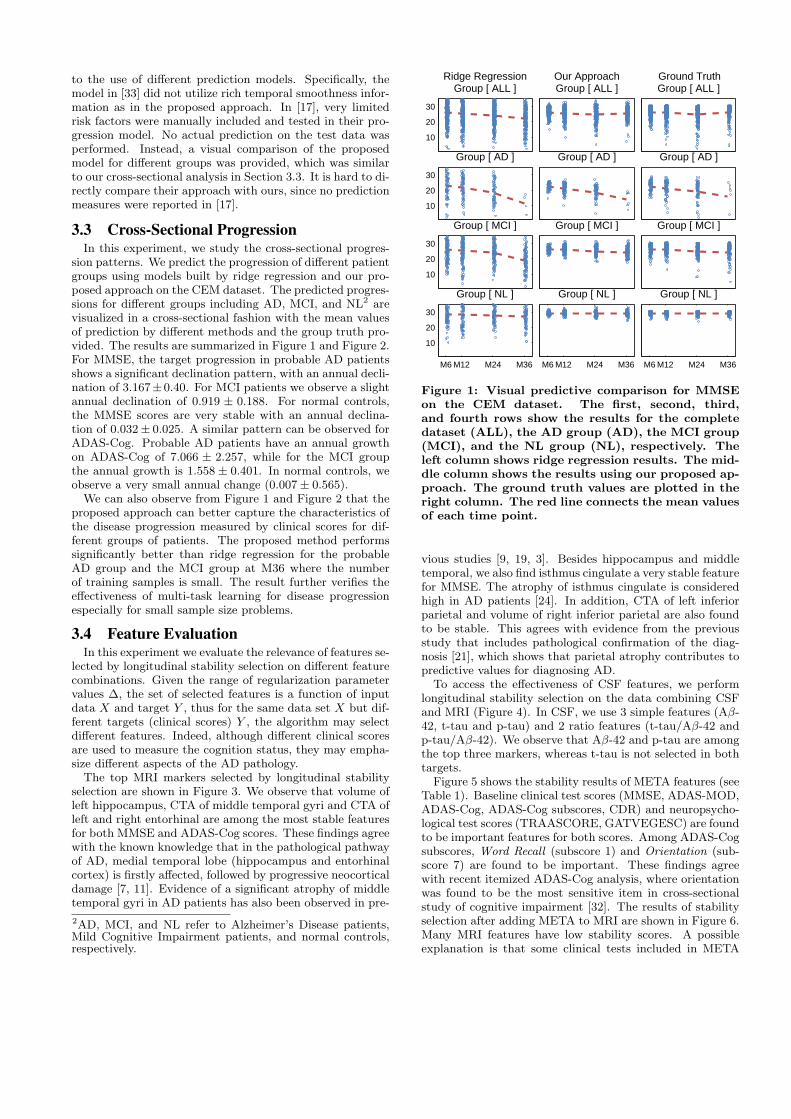
3.2 Prediction PerformanceIn this experiment, we compare our proposed approach

with ridge regression on the prediction of MMSE and ADAS-Cog using various types of data combinations. We reportthe results based on the leave-one-out scheme due to thesmall sample size. 5-fold cross validation is used to selectmodel parameters (θ1, θ2 in our approach and θ1 in ridgeregression) in the training data (between 10−3 and 103).To compare with related works [33, 13], we use correlationcoefficient (R-value) given by the correlation between thepredicted values and the ground truth, and its correlationsignificance (P-value) as the evaluation criteria. P-value isgiven by testing the hypothesis of no correlation [2]. A goodprediction model has a high R-value and low P-value (lessthan 0.0001 for example). The overall performance of theprediction is averaged across all time points weighted by thesample size.The results for MMSE and ADAS-Cog are summarized in

Tables 3 and 4, respectively. Overall, the proposed approach

significantly outperforms ridge regression. This is especiallythe case when the feature space is large and the sample sizeis small, e.g., CM and CEM (see Table 2). Note that multi-task learning effectively increases the number of samples bylearning multiple related tasks simultaneously, while ridgeregression treats all tasks independently. Our results verifythe effectiveness of multi-task learning for disease progres-sion.

Table 3: Comparison of our proposed approach(TGL) and ridge regression (RidR) on longitudinalMMSE prediction using different data combinationsmeasured by R-value and average P-value. Perfor-mance at each time point is reported in terms of R-value. Weighted averages of R-values and P-valuesacross all time points are also given.

M06 M12 M24 M36 AvgR P-Val

CTGL 0.74 0.72 0.71 0.65 0.71 3.3e-026RidR 0.74 0.72 0.71 0.65 0.71 3.3e-026

ETGL 0.83 0.84 0.84 0.78 0.82 7.4e-080RidR 0.82 0.83 0.84 0.76 0.82 2.8e-075

CETGL 0.80 0.82 0.82 0.72 0.80 7.2e-034RidR 0.77 0.80 0.79 0.71 0.77 7.8e-033

MTGL 0.77 0.75 0.77 0.70 0.75 2.7e-059RidR 0.68 0.67 0.71 0.63 0.68 1.2e-045

EMTGL 0.83 0.84 0.85 0.80 0.83 3.8e-088RidR 0.71 0.71 0.74 0.54 0.69 7.1e-032

CMTGL 0.73 0.73 0.76 0.69 0.73 1.3e-030RidR 0.25 0.34 0.36 0.48 0.35 1.0e-006

CEMTGL 0.80 0.83 0.83 0.72 0.80 8.4e-034RidR 0.29 0.36 0.59 0.56 0.43 2.4e-008

Table 4: Comparison of our proposed approach(TGL) and ridge regression (RidR) on longitudinalADAS-Cog prediction using different data combina-tions measured by R-value and average P-value.

M06 M12 M24 M36 AvgR P-Val

CTGL 0.70 0.71 0.71 0.66 0.70 1.7e-026RidR 0.70 0.71 0.70 0.66 0.70 1.5e-026

ETGL 0.87 0.87 0.86 0.83 0.86 2.6e-099RidR 0.87 0.86 0.86 0.83 0.86 4.1e-097

CETGL 0.86 0.85 0.86 0.80 0.85 1.7e-044RidR 0.86 0.84 0.85 0.74 0.83 2.7e-035

MTGL 0.75 0.78 0.76 0.74 0.76 4.4e-066RidR 0.66 0.71 0.67 0.61 0.67 4.9e-041

EMTGL 0.87 0.87 0.86 0.84 0.86 3.2e-104RidR 0.80 0.81 0.80 0.70 0.79 2.4e-058

CMTGL 0.75 0.77 0.75 0.74 0.76 2.5e-035RidR 0.55 0.60 0.62 0.53 0.58 5.4e-016

CEMTGL 0.87 0.86 0.87 0.81 0.86 1.9e-046RidR 0.69 0.66 0.63 0.40 0.62 8.6e-010

In Table 5 we compare our approach with three closelyrelated works. In [13], PCA was employed to reduce thedimensionality of the MRI data. Since only limited sampleswere used, the proposed method resulted in low predictionperformance. To the best of our knowledge, the work in [13]is the only one that tried to predict cognitive scores at futuretime points and reported R/P-Value for comparison. Theother two works used the ADNI database as in our study.Stonnington’s work predicted baseline cognitive scores us-ing relevance vector regression (RVR) which enforced spar-sity in the model [33]. Their regression results were betterthan those reported in [13]. However their prediction per-formance is much lower than ours. This is possibly due

to the use of different prediction models. Specifically, themodel in [33] did not utilize rich temporal smoothness infor-mation as in the proposed approach. In [17], very limitedrisk factors were manually included and tested in their pro-gression model. No actual prediction on the test data wasperformed. Instead, a visual comparison of the proposedmodel for different groups was provided, which was similarto our cross-sectional analysis in Section 3.3. It is hard to di-rectly compare their approach with ours, since no predictionmeasures were reported in [17].

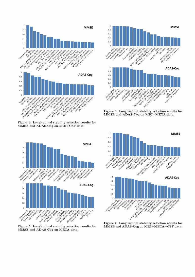
3.3 Cross-Sectional ProgressionIn this experiment, we study the cross-sectional progres-

sion patterns. We predict the progression of different patientgroups using models built by ridge regression and our pro-posed approach on the CEM dataset. The predicted progres-sions for different groups including AD, MCI, and NL2 arevisualized in a cross-sectional fashion with the mean valuesof prediction by different methods and the group truth pro-vided. The results are summarized in Figure 1 and Figure 2.For MMSE, the target progression in probable AD patientsshows a significant declination pattern, with an annual decli-nation of 3.167±0.40. For MCI patients we observe a slightannual declination of 0.919 ± 0.188. For normal controls,the MMSE scores are very stable with an annual declina-tion of 0.032± 0.025. A similar pattern can be observed forADAS-Cog. Probable AD patients have an annual growthon ADAS-Cog of 7.066 ± 2.257, while for the MCI groupthe annual growth is 1.558 ± 0.401. In normal controls, weobserve a very small annual change (0.007± 0.565).We can also observe from Figure 1 and Figure 2 that the

proposed approach can better capture the characteristics ofthe disease progression measured by clinical scores for dif-ferent groups of patients. The proposed method performssignificantly better than ridge regression for the probableAD group and the MCI group at M36 where the numberof training samples is small. The result further verifies theeffectiveness of multi-task learning for disease progressionespecially for small sample size problems.

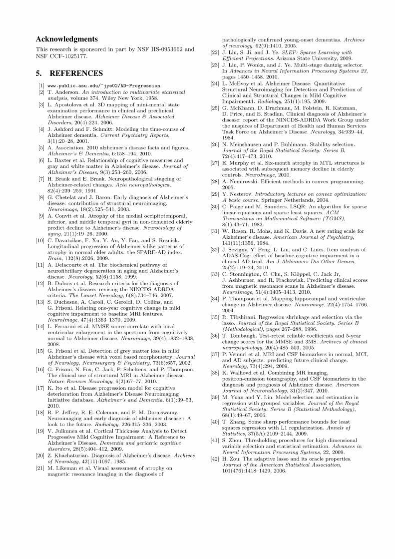
3.4 Feature EvaluationIn this experiment we evaluate the relevance of features se-

lected by longitudinal stability selection on different featurecombinations. Given the range of regularization parametervalues ∆, the set of selected features is a function of inputdata X and target Y , thus for the same data set X but dif-ferent targets (clinical scores) Y , the algorithm may selectdifferent features. Indeed, although different clinical scoresare used to measure the cognition status, they may empha-size different aspects of the AD pathology.The top MRI markers selected by longitudinal stability

selection are shown in Figure 3. We observe that volume ofleft hippocampus, CTA of middle temporal gyri and CTA ofleft and right entorhinal are among the most stable featuresfor both MMSE and ADAS-Cog scores. These findings agreewith the known knowledge that in the pathological pathwayof AD, medial temporal lobe (hippocampus and entorhinalcortex) is firstly affected, followed by progressive neocorticaldamage [7, 11]. Evidence of a significant atrophy of middletemporal gyri in AD patients has also been observed in pre-

2AD, MCI, and NL refer to Alzheimer’s Disease patients,Mild Cognitive Impairment patients, and normal controls,respectively.

10

20

30

Ridge RegressionGroup [ ALL ]

Our ApproachGroup [ ALL ]

Ground TruthGroup [ ALL ]

10

20

30

Group [ AD ] Group [ AD ] Group [ AD ]

10

20

30

Group [ MCI ] Group [ MCI ] Group [ MCI ]

M6 M12 M24 M36

10

20

30

Group [ NL ]

M6 M12 M24 M36

Group [ NL ]

M6 M12 M24 M36

Group [ NL ]

Figure 1: Visual predictive comparison for MMSEon the CEM dataset. The first, second, third,and fourth rows show the results for the completedataset (ALL), the AD group (AD), the MCI group(MCI), and the NL group (NL), respectively. Theleft column shows ridge regression results. The mid-dle column shows the results using our proposed ap-proach. The ground truth values are plotted in theright column. The red line connects the mean valuesof each time point.

vious studies [9, 19, 3]. Besides hippocampus and middletemporal, we also find isthmus cingulate a very stable featurefor MMSE. The atrophy of isthmus cingulate is consideredhigh in AD patients [24]. In addition, CTA of left inferiorparietal and volume of right inferior parietal are also foundto be stable. This agrees with evidence from the previousstudy that includes pathological confirmation of the diag-nosis [21], which shows that parietal atrophy contributes topredictive values for diagnosing AD.

To access the effectiveness of CSF features, we performlongitudinal stability selection on the data combining CSFand MRI (Figure 4). In CSF, we use 3 simple features (Aβ-42, t-tau and p-tau) and 2 ratio features (t-tau/Aβ-42 andp-tau/Aβ-42). We observe that Aβ-42 and p-tau are amongthe top three markers, whereas t-tau is not selected in bothtargets.

Figure 5 shows the stability results of META features (seeTable 1). Baseline clinical test scores (MMSE, ADAS-MOD,ADAS-Cog, ADAS-Cog subscores, CDR) and neuropsycho-logical test scores (TRAASCORE, GATVEGESC) are foundto be important features for both scores. Among ADAS-Cogsubscores, Word Recall (subscore 1) and Orientation (sub-score 7) are found to be important. These findings agreewith recent itemized ADAS-Cog analysis, where orientationwas found to be the most sensitive item in cross-sectionalstudy of cognitive impairment [32]. The results of stabilityselection after adding META to MRI are shown in Figure 6.Many MRI features have low stability scores. A possibleexplanation is that some clinical tests included in META

Table 5: Comparison of the proposed approach with three related works in the literature. AD, MCI, and NLrefer to Alzheimer’s Disease patients, Mild Cognitive Impairment patients, and normal controls, respectively.

Method Target Subjects Feature ResultDuchesne et al. [13] M06 MMSE 75 NL, 49 MCI, 75 AD Baseline MRI, age,

gender, years of educa-tion

MMSE: 0.31 (p=0.03)

Stonnington et al. [33] baselineMMSE andADAS-Cog

Set1: 73 AD, 91 NLSet2 (ADNI): 113 AD,351 MCI, 122 NL

Baseline MRI, CSF MMSE: Set1: 0.7 (p<10e-5) Set2:0.48 (p<10e-5) ADAS-Cog: Set2:0.57 (p<10e-5)

Ito et al. [17] M06-M36ADAS-Cog

ADNI: 186 AD, 402MCI, 229 NL

Age, APOE4, gender,family history, years ofeducation

Only visual check. R/P value notreport

Our approach M06-M36MMSE andADAS-Cog

ADNI: 133 AD, 304MCI, 188 NL

Baseline MRI, CSF,and META (see Table1 for details)

Avg MMSE: 0.83 (p=3.8e-88)Avg ADAS-Cog: 0.86(p=3.2e-104)

20

40

60

Ridge RegressionGroup [ ALL ]

Our ApproachGroup [ ALL ]

Ground TruthGroup [ ALL ]

20

40

60

Group [ AD ] Group [ AD ] Group [ AD ]

20

40

60

Group [ MCI ] Group [ MCI ] Group [ MCI ]

M6 M12 M24 M36

20

40

60

Group [ NL ]

M6 M12 M24 M36

Group [ NL ]

M6 M12 M24 M36

Group [ NL ]

Figure 2: Visual predictive comparison for ADAS-Cog on the CEM dataset.

features reflect white matter and/or gray matter changes,as discussed in [6].Next we perform stability selection by adding all three

types of features together. Results are shown in Figure 7.We can observe from the figure that there are many featuresin common for both targets: baseline ADAS-Cog, ADAS-MOD and MMSE; baseline ADAS-Cog subscores 1 and 7;Logic LIMMTOTAL; APOE and DIGITSCOR.

4. CONCLUSIONIn this paper, we study the feasibility of predicting AD

progression measured by cognitive scores based on baselinemeasurements. Specifically, we formulate the progressionprediction as a multi-task regression problem by consider-ing the prediction of cognitive scores at each time point asa task. To capture the intrinsic relatedness among differ-ent tasks at different time points, we propose a temporalgroup Lasso regularizer, which ensures a small deviation be-tween two regression models at successive time points basedon a small subset of features. The effectiveness of the pro-

0

0.2

0.4

0.6

0.8

1

MMSE

0

0.2

0.4

0.6

0.8

1

ADAS-Cog

Figure 3: Longitudinal stability selection results forMMSE and ADAS-Cog on MRI data.

posed approach in predicting disease progression and featureselection is evaluated by extensive experimental studies onthe ADNI database. Results show that the proposed ap-proach can better capture the progression trends than exist-ing methods. Results also show that most features selectedby the proposed approach are consistent with findings fromexisting cross-sectional studies. Our experimental studiesdemonstrate the promise of multi-task learning for predict-ing disease progression.

Our proposed formulation for AD progression predictionand feature selection is able to deal with missing values in thetarget matrix. Missing values in the input matrix, however,cannot be handled. Recent advances on matrix completionhave allowed us to complete matrices with many missingvalues under certain conditions. We will explore such tech-niques for dealing with missing values in the input data. Inaddition, in this study we only focus on linear models; weplan to explore non-linear models in the future.

0

0.2

0.4

0.6

0.8

1

MMSE

0

0.2

0.4

0.6

0.8

1

ADAS-Cog

Figure 4: Longitudinal stability selection results forMMSE and ADAS-Cog on MRI+CSF data.

0

0.2

0.4

0.6

0.8

1

MMSE

0

0.2

0.4

0.6

0.8

1

ADAS-Cog

Figure 5: Longitudinal stability selection results forMMSE and ADAS-Cog on META data.

0

0.2

0.4

0.6

0.8

1

MMSE

0

0.2

0.4

0.6

0.8

1ADAS-Cog

Figure 6: Longitudinal stability selection results forMMSE and ADAS-Cog on MRI+META data.

0

0.2

0.4

0.6

0.8

1MMSE

0

0.2

0.4

0.6

0.8

1 ADAS-Cog

Figure 7: Longitudinal stability selection results forMMSE and ADAS-Cog on MRI+META+CSF data.

AcknowledgmentsThis research is sponsored in part by NSF IIS-0953662 andNSF CCF-1025177.

5. REFERENCES[1] www.public.asu.edu/~jye02/AD-Progression.

[2] T. Anderson. An introduction to multivariate statisticalanalysis, volume 374. Wiley New York, 1958.

[3] L. Apostolova et al. 3D mapping of mini-mental stateexamination performance in clinical and preclinicalAlzheimer disease. Alzheimer Disease & AssociatedDisorders, 20(4):224, 2006.

[4] J. Ashford and F. Schmitt. Modeling the time-course ofAlzheimer dementia. Current Psychiatry Reports,3(1):20–28, 2001.

[5] A. Association. 2010 alzheimer’s disease facts and figures.Alzheimer’s & Dementia, 6:158–194, 2010.

[6] L. Baxter et al. Relationship of cognitive measures andgray and white matter in Alzheimer’s disease. Journal ofAlzheimer’s Disease, 9(3):253–260, 2006.

[7] H. Braak and E. Braak. Neuropathological stageing ofAlzheimer-related changes. Acta neuropathologica,82(4):239–259, 1991.

[8] G. Chetelat and J. Baron. Early diagnosis of Alzheimer’sdisease: contribution of structural neuroimaging.Neuroimage, 18(2):525–541, 2003.

[9] A. Convit et al. Atrophy of the medial occipitotemporal,inferior, and middle temporal gyri in non-demented elderlypredict decline to Alzheimer’s disease. Neurobiology ofaging, 21(1):19–26, 2000.

[10] C. Davatzikos, F. Xu, Y. An, Y. Fan, and S. Resnick.Longitudinal progression of Alzheimer’s-like patterns ofatrophy in normal older adults: the SPARE-AD index.Brain, 132(8):2026, 2009.

[11] A. Delacourte et al. The biochemical pathway ofneurofibrillary degeneration in aging and Alzheimer’sdisease. Neurology, 52(6):1158, 1999.

[12] B. Dubois et al. Research criteria for the diagnosis ofAlzheimer’s disease: revising the NINCDS-ADRDAcriteria. The Lancet Neurology, 6(8):734–746, 2007.

[13] S. Duchesne, A. Caroli, C. Geroldi, D. Collins, andG. Frisoni. Relating one-year cognitive change in mildcognitive impairment to baseline MRI features.NeuroImage, 47(4):1363–1370, 2009.

[14] L. Ferrarini et al. MMSE scores correlate with localventricular enlargement in the spectrum from cognitivelynormal to Alzheimer disease. Neuroimage, 39(4):1832–1838,2008.

[15] G. Frisoni et al. Detection of grey matter loss in mildAlzheimer’s disease with voxel based morphometry. Journalof Neurology, Neurosurgery & Psychiatry, 73(6):657, 2002.

[16] G. Frisoni, N. Fox, C. Jack, P. Scheltens, and P. Thompson.The clinical use of structural MRI in Alzheimer disease.Nature Reviews Neurology, 6(2):67–77, 2010.

[17] K. Ito et al. Disease progression model for cognitivedeterioration from Alzheimer’s Disease NeuroimagingInitiative database. Alzheimer’s and Dementia, 6(1):39–53,2010.

[18] R. P. Jeffrey, R. E. Coleman, and P. M. Doraiswamy.Neuroimaging and early diagnosis of alzheimer disease : Alook to the future. Radiology, 226:315–336, 2003.

[19] V. Julkunen et al. Cortical Thickness Analysis to DetectProgressive Mild Cognitive Impairment: A Reference toAlzheimer’s Disease. Dementia and geriatric cognitivedisorders, 28(5):404–412, 2009.

[20] Z. Khachaturian. Diagnosis of Alzheimer’s disease. Archivesof Neurology, 42(11):1097, 1985.

[21] M. Likeman et al. Visual assessment of atrophy onmagnetic resonance imaging in the diagnosis of

pathologically confirmed young-onset dementias. Archivesof neurology, 62(9):1410, 2005.

[22] J. Liu, S. Ji, and J. Ye. SLEP: Sparse Learning withEfficient Projections. Arizona State University, 2009.

[23] J. Liu, P. Wonka, and J. Ye. Multi-stage dantzig selector.In Advances in Neural Information Processing Systems 23,pages 1450–1458. 2010.

[24] L. McEvoy et al. Alzheimer Disease: QuantitativeStructural Neuroimaging for Detection and Prediction ofClinical and Structural Changes in Mild CognitiveImpairment1. Radiology, 251(1):195, 2009.

[25] G. McKhann, D. Drachman, M. Folstein, R. Katzman,D. Price, and E. Stadlan. Clinical diagnosis of Alzheimer’sdisease: report of the NINCDS-ADRDA Work Group underthe auspices of Department of Health and Human ServicesTask Force on Alzheimer’s Disease. Neurology, 34:939–44,1984.

[26] N. Meinshausen and P. Buhlmann. Stability selection.Journal of the Royal Statistical Society: Series B,72(4):417–473, 2010.

[27] E. Murphy et al. Six-month atrophy in MTL structures isassociated with subsequent memory decline in elderlycontrols. NeuroImage, 2010.

[28] A. Nemirovski. Efficient methods in convex programming.2005.

[29] Y. Nesterov. Introductory lectures on convex optimization:A basic course. Springer Netherlands, 2004.

[30] C. Paige and M. Saunders. LSQR: An algorithm for sparselinear equations and sparse least squares. ACMTransactions on Mathematical Software (TOMS),8(1):43–71, 1982.

[31] W. Rosen, R. Mohs, and K. Davis. A new rating scale forAlzheimer’s disease. American Journal of Psychiatry,141(11):1356, 1984.

[32] J. Sevigny, Y. Peng, L. Liu, and C. Lines. Item analysis ofADAS-Cog: effect of baseline cognitive impairment in aclinical AD trial. Am J Alzheimers Dis Other Demen,25(2):119–24, 2010.

[33] C. Stonnington, C. Chu, S. Kloppel, C. Jack Jr,J. Ashburner, and R. Frackowiak. Predicting clinical scoresfrom magnetic resonance scans in Alzheimer’s disease.NeuroImage, 51(4):1405–1413, 2010.

[34] P. Thompson et al. Mapping hippocampal and ventricularchange in Alzheimer disease. Neuroimage, 22(4):1754–1766,2004.

[35] R. Tibshirani. Regression shrinkage and selection via thelasso. Journal of the Royal Statistical Society. Series B(Methodological), pages 267–288, 1996.

[36] T. Tombaugh. Test-retest reliable coefficients and 5-yearchange scores for the MMSE and 3MS. Archives of clinicalneuropsychology, 20(4):485–503, 2005.

[37] P. Vemuri et al. MRI and CSF biomarkers in normal, MCI,and AD subjects: predicting future clinical change.Neurology, 73(4):294, 2009.

[38] K. Walhovd et al. Combining MR imaging,positron-emission tomography, and CSF biomarkers in thediagnosis and prognosis of Alzheimer disease. AmericanJournal of Neuroradiology, 31(2):347, 2010.

[39] M. Yuan and Y. Lin. Model selection and estimation inregression with grouped variables. Journal of the RoyalStatistical Society: Series B (Statistical Methodology),68(1):49–67, 2006.

[40] T. Zhang. Some sharp performance bounds for leastsquares regression with L1 regularization. Annals ofStatistics, 37(5A):2109–2144, 2009.

[41] S. Zhou. Thresholding procedures for high dimensionalvariable selection and statistical estimation. Advances inNeural Information Processing Systems, 22, 2009.

[42] H. Zou. The adaptive lasso and its oracle properties.Journal of the American Statistical Association,101(476):1418–1429, 2006.