a multivariate generalized independent factor garch model with an application to financial stock...

7/26/2019 A Multivariate Generalized Independent Factor GARCH Model With an Application to Financial Stock Returns

http://slidepdf.com/reader/full/a-multivariate-generalized-independent-factor-garch-model-with-an-application 1/24

Working Paper 08-75

Statistics and Econometrics Series 28

December 2008

Departamento de Estadística

Universidad Carlos III de Madrid

Calle Madrid, 126

28903 Getafe (Spain)

Fax (34) 91 624-98-49

A MULTIVARIATE GENERALIZED INDEPENDENT FACTOR GARCH

MODEL WITH AN APPLICATION TO FINANCIAL STOCK RETURNS

Antonio García-Ferrer 1, Ester González-Prieto2, and Daniel Peña3

Abstract

We propose a new multivariate factor GARCH model, the GICA-GARCH model ,

where the data are assumed to be generated by a set of independent components (ICs).

This model applies independent component analysis (ICA) to search the conditionally

heteroskedastic latent factors. We will use two ICA approaches to estimate the ICs. The

first one estimates the components maximizing their non-gaussianity, and the second

one exploits the temporal structure of the data. After estimating the ICs, we fit anunivariate GARCH model to the volatility of each IC. Thus, the GICA-GARCH reduces

the complexity to estimate a multivariate GARCH model by transforming it into a small

number of univariate volatility models. We report some simulation experiments to show

the ability of ICA to discover leading factors in a multivariate vector of financial data.

An empirical application to the Madrid stock market will be presented, where we

compare the forecasting accuracy of the GICA-GARCH model versus the orthogonal

GARCH one.

Keywords: ICA, Multivariate GARCH, Factor Models, Forecasting Volatility

1 Departamento de Análisis Económico: Economía Cuantitativa. Universidad Autónoma de

Madrid, C/ Francisco Tomás y Valiente 5, 28049 Cantoblanco (Madrid), e-mail:[email protected] 2 Departamento de Estadística. Universidad Carlos III de Madrid, C/ Madrid 126, 28903 Getafe(Madrid), e-mail: [email protected] 3

Departamento de Estadística. Universidad Carlos III de Madrid, C/ Madrid 126, 28903 Getafe(Madrid), e-mail: [email protected]



A multivariate generalized independent factor GARCH model

with an application to financial stock returns

Antonio Garcıa-Ferrer∗, Ester Gonzalez-Prieto†, and Daniel Pena‡

December 2008

Abstract

We propose a new multivariate factor GARCH model, the GICA-GARCH model, where

the data are assumed to be generated by a set of independent components (ICs). This model

applies independent component analysis (ICA) to search the conditionally heteroskedastic

latent factors. We will use two ICA approaches to estimate the ICs. The first one estimates

the components maximizing their non-gaussianity, and the second approach exploits the

temporal structure of the data. After estimating the ICs, we fit an univariate GARCH

model to the volatility of each IC. Thus, the GICA-GARCH reduces the complexity to

estimate a multivariate GARCH model by transforming it into a small number of univariate

volatility models. We report some simulation experiments to show the ability of ICA to

discover leading factors in a multivariate vector of financial data. An empirical applicationto the Madrid stock market will be presented, where we compare the forecasting accuracy of

the GICA-GARCH model versus the orthogonal GARCH one.

Keywords: ICA, Multivariate GARCH, Factor Models, Forecasting Volatility.

1 Introduction

Since Engel (1982) introduced the ARCH model and Bollerslev (1986) generalized it, proposing

the GARCH model, many researchers have been interested in modelling volatility in finan-

cial time series. In multivariate time series, financial volatilities tend to move together across

markets, and in order to understand their comovements, a multivariate modelling approach is

required. The first multivariate GARCH model (MGARCH) was proposed by Bollerslev, En-

gle and Wooldridge (1988) as an extension of the univariate GARCH model. Other different

specifications for MGARCH have been proposed in the literature (see, for example, the sur-

vey of Bauwens et al., 2006), but in these developments the number of parameters to estimate

∗Departamento de Analisis Economico: Economıa Cuantitativa. Universidad Autonoma de Madrid. E-mail:

[email protected]†Departamento de Estadıstica. Universidad Carlos III de Madrid. E-mail: [email protected]‡Departamento de Estadıstica. Universidad Carlos III de Madrid. E-mail: [email protected]

1



Garcıa-Ferrer, Gonzalez-Prieto & Pe˜ na 2

can be very large, and the restrictions to guarantee the positive definiteness of the conditional

covariance matrix are difficult to implement. A possible solution to these problems is to use

factor models, where the data set are explained by a small number of unobserved components.

Comovements in stock returns reinforce the intuition that financial markets are driven by a few

latent common sources.

Several factor models have been presented in the literature. The most popular one is the

orthogonal GARCH model (O-GARCH) (Alexander, 2001) that estimates the unobserved factors

using a small set of principal components (PCs), and fits an univariate GARCH model for

each component. That is, the O-GARCH estimates a MGARCH model requiring only a small

number of univariate GARCH estimations. Van der Weide (2002) introduces a vectorized version

of the O-GARCH, the generalized orthogonal GARCH model (GO-GARCH), that does not

reduce the dimension of the data and does not allow for idiosyncratic components. In order

to solve these problems, Lanne and Saikkonen (2007) propose the generalized orthogonal factor

GARCH model, that allows some diagonal elements of the conditional covariance matrix to

be constant. All previous models use principal components analysis (PCA) to identify theset of underlying factors, which are unconditionally uncorrelated. However, to guarantee the

diagonality of the conditional covariance matrix, an additional assumption is needed: the factors

must be conditionally uncorrelated. Fan et al. (2008) show that this assumption could lead

to serious errors in model fitting, and they propose to model multivariate volatilities using

conditionally uncorrelated components (CUC-GARCH).

In this paper we propose a new alternative for modelling multivariate volatilities as linear com-

bination of several univariate GARCH models. We introduce a multivariate generalized inde-

pendent component analysis GARCH model (GICA-GARCH). Independent component analysis

(ICA) can be seen as a factor model (Hyv arinen and Kano, 2003) where the unobserved com-

ponents are non-gaussian, and mutually independent. Previous researchers, Back and Weigend

(1997), Kiviluoto and Oja (1998), Cha and Chan (2000), and M alaroiu et al. (2000) among oth-

ers, have applied ICA to financial data. Furthermore, ICA can be considered as a generalization

of PCA (Hyvarinen et al., 2001), and seems to be, a priori, more suitable than PCA to explain

the non-gaussian behaviour of financial data (Wu and Yu, 2005).

The key idea of the GICA-GARCH is to assume that financial data are generated by a linear

combination of a small number of conditionally heteroskedastic independent components and

idiosyncratic shocks. Then, GICA-GARCH can be seen as a generalization of the multivariateGARCH model proposed by Lanne and Saikkonen (2007), but assuming that the unobserved

factors are estimated by ICA rather than by PCA. Therefore, the common components will be

unconditionally independent and not only uncorrelated. Moreover, the GICA-GARCH is related

to the O-GARCH because both models transform the problem of estimating a multivariate

GARCH model into a small number of univariate GARCH models. Finally, note that the

independence assumption of the GICA-GARCH model is stronger than the one corresponding

to the CUC-GARCH model.

The paper is organized as follows. In Section 2 we present the ICA model, describe the

three ICA algorithms that we apply to estimate the unobserved components, and explain aprocedure to sort the ICA components in terms of their explained variability. Furthermore,

the relationship between ICA and dynamic factor model (DFM) is analyzed. In Section 3, we

introduce the GICA-GARCH model and its application to forecast the volatility of a vector of




stock returns from the volatility of a small number of components. Some simulation experiments

to illustrate the ability of this model to estimate the unobserved components are presented in

Section 4. Section 5 shows the results of the empirical application to a real-time dataset. Finally,

Section 6 gives some concluding remarks.

2 The ICA model

In this section, we introduce the concept of ICA. First, we present the basic ICA model according

to the formal definition given by Common (1994). Then, we briefly describe the three algorithms

we use to estimate the ICA components. As the definition of ICA implies no ordering of the ICs,

a procedure to weight and sort them is next explained. Finally, we formulate the ICA model as

a particular DFM and analyze the relationship between both models.

2.1 Definition of ICA

ICA assumes that the observed multivariate vector is a linear combination of a set of unobserved

components. Let xt = (x1t, x2t, . . . , xmt) be the m−dimensional vector of stationary time series,

with E [xt] = 0 and E [xtxt] = Γx (0) positive definite. We assume that xt is generated by a

linear combination of r (r ≤ m) latent factors. That is,

xt = Ast, t = 1, 2,...,T (1)

where A is an unknown m × r full rank matrix, with elements aij that represent the effect

of s

jt on x

it, for i

= 1,

2,...,m

and j

= 1,

2,...,r

, and s

t = (s

1t, s

2t, . . . , s

rt)

is the vector of unobserved factors, which are called independent components (ICs). We assume that E [st] = 0,

E [stst] = Ir, and the components of st are statistically independent. Let (x1, x2, ..., xT ) be

the observed multivariate time series. The problem is to estimate both A and st only from

(x1, x2, ..., xT ) . That is, ICA looks for an r ×m matrix, W, such that the components given by

st = Wxt, t = 1, 2,...,T, (2)

are as independent as possible. However, previous assumptions are not sufficient to estimate A

and st uniquely, and it is required that no more than one IC is normally distributed. By (1) ,

we have:

Γx (0) = AA, (3)

Γx (τ ) = AΓs (τ ) A, for τ ≥ 1.

Note that, in spite of previous assumptions, ICA cannot determine either the sign or the

order of the ICs. From now, through this paper, we focus on the most basic form of ICA, which

considers that the number of observed variables is equal to the number of unobserved factors,

i.e., m = r.

2.2 Procedures for estimating the ICs

Both ICA and PCA obtain the latent factors as linear combinations of the data. However their

aims are slightly different. PCA tries to get uncorrelated factors and, for this purpose, it requires




the matrix W such that WW = I, and the rows of W are the projection vectors that maximize

the variance of the estimated unobserved factors, st. On the other hand, the most often used

methods for estimating the ICs impose the restriction that the rows of W are the directions

that maximize the independence of

st.

Three main ICA algorithms have been proposed: JADE (Cardoso and Souloumiac, 1993) and

FastICA (Hyvarinen, 1999; Hyvarinen and Oja, 1997) are based on the non-gaussianity of the

ICs, while SOBI (Belouchrani et al., 1997) is based on the temporal independence of the data.

Before the application of any of these algorithms, it is useful to standardize the data. Thus, we

search for a linear transformation of xt, zt = Mxt, where M is an m × m matrix such that the

m−dimensional vector zt has identity covariance matrix. This multivariate standardization is

carried out as follows. From

Γx (0) = E xtxt = EDE, (4)

where Em×m is the orthogonal matrix of eigenvectors, and Dm×m the diagonal matrix of eigen-

values, then M = D−1/2E. The model (1) in terms of zt, is

zt = Ust, (5)

where U = MA is, by (3) and (4) , an m × m orthogonal matrix. Therefore, the multivariate

standardization of the original data guarantees the orthogonality of the loading matrix.

2.2.1 Joint Approximate Diagonalization of Eigen-matrices: JADE

JADE (Cardoso and Souloumiac, 1993) estimates the ICs maximizing their non-gaussianity.

After whitening the observed data, JADE looks for a matrix, U = (MA), such that thecomponents given by sJ

t = Uzt, (6)

are maximally non-gaussian distributed. Under the non-gaussianity assumption, the information

provided by the covariance matrix of the data, Γz (0) = E ztzt = I, is not sufficient to compute

(6), and higher-order information is needed. Cardoso and Souloumiac (1993) use the cumulants,

which are the coefficients of the Taylor series expansion of the characteristic function. In practice,

it is enough to take into account fourth-order cumulants, which are defined as:

cum4(zit, z jt , zht, zlt) = E zitz jtzhtzlt − E zitz jtE zhtzlt − (7)

−E zitzhtE z jt zlt − E zitzltE z jtzht ,

and the fourth-order cumulant tensor associated to zt is a m × m matrix given by

[Qz (Q)]ij =r

k,l=1

cum4 (zit, z jt, zkt, zlt) q kl,

where Q = (q kl)mk,l=1 is an arbitrary m

×m matrix, and cum4 (zi, z j , zk, zl) is like in (7) . It is easy

to see that a set of random vectors is independent if all their cross-cumulants of order higher

than two are equal to zero. Therefore, sJ t will be maximally independent if its associated fourth

order cumulant tensor, Q sJ t(·) , is maximally diagonal. Cardoso and Soloumiac (1993) show that

given a set of m × m matrices, = Q1, · · · , Qq , there exists an orthogonal transformation,




V, such that the matrices VQz (Qi) VQi∈ are approximately diagonal. Then V = U, and

the latent factors are estimated as in (6) . JADE uses an iterative process of Jacobi rotations

to solve the joint diagonalization of several cumulants matrices. It is a very efficient algorithm

in low dimensional problems, but when the dimension increases, it requires high computational

cost.

2.2.2 Fast Fixed-Point Algorithm: FastICA

FastICA is a fixed-point algorithm for non-adaptative environments, which was proposed by

Hyvarinen and Oja (1997). It estimates

sF t = Uzt (8)

by maximizing their kurtosis. Thus, FastICA searches the directions of projection that maximize

the absolute value of the kurtosis of the sF t . As kurtosis is very sensitive to outliers, FastICA

is not a robust algorithm. Hyvarinen (1999) proposes a more robust version of FastICA using

an approximation of negentropy instead of kurtosis to measure the non-gaussianity of the ICs.

Negentropy is the normalized version of entropy given by:

J sF

t

= H ( sg

t ) − H sF

t

,

where sgt is a gaussian vector of the same correlation matrix as sF

t , and H (·) is the entropy of

a random vector defined as H sF

t

= −E

log p sF t

(ξ )

, where p sF t(·) is the density function of

sF

t . Negentropy is a good index for non-gaussianity because it is always non-negative and it is

zero iff the variable is gaussian distributed. Therefore, the ICs, given by (8), are estimated as

the projections of the data in the directions such that the negentropy of sF t is maximum. The

main advantage of FastICA is that it converges in a few number of iterations.

2.2.3 Second-Order Blind Identification: SOBI

Belouchrani et al. (1997) extended the previous work of Tong et al. (1990), and proposed the

SOBI algorithm. SOBI requires that the ICs, given by

sS t = Uzt, (9)

will be mutually uncorrelated for a set of time lags. That is, a set of time delayed covariance

matrices of sS t ,

Γs (τ ) = E sS

t sS t−τ

, for τ ≥ 1, (10)

should be diagonal. SOBI searches for an orthogonal transformation that jointly diagonalizes

(10) . This algorithm also applies whitening as a preprocessing procedure, and the covariance

structure of the whitened data model (5) is given by:

Γz (τ ) = UΓs (τ ) U, for τ ≥ 1, (11)

where U is an orthogonal matrix. Therefore,

Γs (τ ) = UΓz (τ ) U, for τ ≥ 1. (12)




Thus, SOBI searches for an orthogonal transformation that will be the joint diagonalizer of the

set of time delayed covariance matrices, Γs (τ q)τ q∈ . The optimization problem is to minimize

F (U) =τ q∈

off

UΓz (τ ) U

,

where

off

is a measure of the non-diagonality of a matrix, which is defined by the sum of the squares of their off-diagonal elements. SOBI solves this problem using Jacobi rotation

techniques. Belouchrani et al. (1997) show that this problem has a unique solution: if there

exists two different ICs that have different autocovariances for at least one time-lag, then the

joint diagonalizer, U, exists and it is unique. That is, if for all 1 ≤ i = j ≤ r, there is any

q = 1,...,K such that γ si (τ q) = γ sj (τ q) , then the components of sS t can be separated, they

are unique, and lagged uncorrelated. Note that SOBI cannot get the ICs if they have identical

autocovariances for the lags considered.

2.2.4 Weighting the ICs

After estimating the components, we should decide which of them are more important to explain

the underlying structure of the observed data. Note that the PCs are sorted in terms of vari-

ability, but the ICs are undeterminated with respect to the order. Following Back and Weigend

(1997), we sort the ICs in terms of their explained variability. According to model (1) , the ith

observed variable is given by xit = m

j=1 aijs jt, and its variance is

var(xit) =m

i=1

a2ij, ∀ i = 1,...,m. (13)

For each xit, with i = 1,...,m, Back and Weigend (1997) define the weighted ICs in terms of

the elements of the ith row of A as sw(i)t = diag (ai1, ai2, . . . , aim) st. That is, for each xit, the

jth weighted IC is given by sw(i) jt = aijs jt, for j = 1,...,m, and its variance is

var

sw(i) jt

= a2

ij, ∀ i, j = 1,...,m. (14)

Therefore, from (13) and (14) , the variance of xit which is explained by sw(i) jt is computed as:

ν i

j =

a2ijm

i=1 a2ij

. (15)

The total variance of xt explained by the j th IC is given by:

ϑ j =

mi=1 ν i jm

j=1

mi=1 ν i j

, ∀ j = 1,...,m.

Thus, after getting ϑ1, ϑ2,...,ϑm, we can sort the ICs in terms of variability. The most

important ICs will be those that explain the maximum variance of xt.

2.3 ICA and the Dynamic Factor Model

Suppose that, in the basic ICA model, there are r gaussian components, s(1)t = (s1t, . . . , srt) with

r < m, representing the common dynamic of the time series, but the other m − r components,




s(2)t = (sr+1t, . . . , smt) , are Gaussian. Then we can split the matrix A = [A1A2] accordingly

and write

xt = A1s(1)t + A2s

(2)t . (16)

Calling nt = A2s(2)t to the vector of Gaussian noise we have xt = A1s

(1)t + nt, which is similar

to the DFM studied by Pena and Box (1987). However, there are two main differences between

these models. First, in the factor model, the r common factors, s(1)t , are assumed Gaussian

and linear, whereas here they are non Gaussian. Second, in the standard factor model the

covariance matrix of the noise is of full rank, whereas here it will have rank equal to m − r.

This last constraint can be relaxed by assuming that the ICA model is contaminated with some

Gaussian error model, as in xt = Ast + u, where u is Gaussian. Note that the latent factors of

the DFM can be estimated by using PCA (see, for example, Stock and Watson, 2002).

3 The GICA-GARCH model

This section presents the GICA-GARCH model as a new multivariate volatility model. From

now on, let xt = (x1t, x2t, . . . , xmt) be the vector of m financial time series. First, we introduce

the GICA-GARCH model, give its mathematical formulation, and describe the structure of the

ICA components. Then, we explain how our model is used to forecast the volatility of a vector

of financial data from the volatility of a set of ICs. Finally, we relate the GICA-GARCH model

to other factor GARCH models. In particular, we show that the GICA-GARCH model can be

seen as a particular dynamic factor GARCH model.

3.1 The model

Empirical evidence reveals that financial assets cannot be predicted at short horizons, but it is

well known that we can forecast their conditional variance using a particular GARCH model

(Engel, 1982; Bollerslev, 1986). Therefore, we focus our analysis on forecasting the volatility

of the observed financial time series. Let us assume that xt is a linear combination of a set

of independent factors given by (1) . Financial time series are characterized by the presence

of clusters of volatility, and this implies that the unobserved factors will follow conditionally

heteroskedastic processes. We suppose that the vector of unobserved components, st, follows an

r-dimensional ARMA( p, q ) model with GARCH ( p, q ) disturbances:

st =

pi=1

Φist−i +

ql=0

Θlet−l, (17)

where Φi = diag

φ(1)i ,...,φ

(r)i

with |φ( j)

i | < 1 ∀ j, Θl = diag

θ(1)l ,...,θ

(r)l

with Θ0 = Ir and

|θ( j)l | < 1 ∀ j, and et is an r-dimensional vector of conditionally heteroskedastic errors given by:

et = H1/2t εt, (18)

where εt ∼ iid (0, Ir) and H1/2

t = diag( h jt) is an r × r positive definite diagonal matrix suchthat

h jt = α( j)0 +

pi=1

α( j)i e2

jt−i +

ql=1

β ( j)l h jt−l, for j = 1,..,r, (19)




where h jt is a stationary process, independent of ε jt , and it is the conditional variance of the

jth IC: h jt = V (e jt |It−1) = V (s jt |It−1) , where It−1 is the past information available until time

t − 1. In order to ensure a positive h jt > 0, ∀ j, it is assumed that α( j)0 > 0, α

( j)i ≥ 0, β

( j)i ≥ 0,

and max( p,q)

i=1

α

( j)i + β

( j)i

< 1 (see Bollerslev, 1986).

From (1) , we have that the conditional covariance matrix of xt is:

Ωt = V (xt|It−1) = AHtA, (20)

where Ht = diag(h1t,...,hrt) is the r ×r conditional covariance matrix of st at time time t. That

is, we can forecast the volatility of the stock returns from the predicted volatility of the com-

ponents. Note that we have assumed that Ht is diagonal, but the ICs are only unconditionally

independent. In order to guarantee the diagonality of Ht, we should assume that the conditional

correlations of the ICs are zero. This assumption allows us to achieve our purpose: estimating a

multivariate GARCH model from a small number of GARCH univariate models, and therefore,

reducing considerably the number of parameters to be estimated.

3.2 Identification of the factors

In practice, we separate the estimation of the factors from fitting their volatility models. First,

we apply ICA to identify the underlying independent components. Any of the previous ICA

algorithms standardizes the data as a preprocessing step, and solves the basic ICA model for

the normalized data, which is given by equation (5). Thus, JADE, FastICA, and SOBI will

estimate the loading matrix, that is orthogonal, and the m ICs, defined by equation (6) , (8) ,

and (9) , respectively. After estimating the model, we weight the ICs according to the procedure

explained in (2.2.4.): we sort the ICs in terms of their explained total variability and the first

few are the most important ICs. Hence, we split the vector of ICs as st = [s(1)t s

(2)t ], where s

(1)t =

(s1t, . . . , srt) are the r ICs, with r < m, which we choose to represent the data, and s(2)t =

(sr+1t, . . . , smt) are the m − r ICs which we consider as noise. From now on, we focus on the r

selected ICs and we fit an univariate ARMA( p, q ) − GARCH ( p, q ) for each one of them. We

estimate the univariate volatility of each IC and generate the conditional covariance matrix of

s(1)t , Ht. Finally, we get the conditional covariance matrix of the observed data from (20) and

its ith diagonal term, γ 2it =

r j=1 h jta2

ij, is the conditional variance of xit, for i = 1, 2,...,m.

Note that the performance of the GICA-GARCH model depends on the method we apply toestimate the ICs. We will investigate the usefulness of the three algorithms presented in section

2. Since we have seen that they use different estimation principles (JADE and FastICA non-

gaussianity, and SOBI dynamic uncorrelation) the performance of the algorithms is expected to

depend on the features of the data.

Financial data usually tend to exhibit fat-tailed distributions. The kurtosis coefficient is a

popular measure for the thickness of the tails and financial data have excess kurtosis. Fur-

thermore, they have small lagged autocorrelation coefficients. Then, it seems that JADE and

FastICA could work better for financial data than SOBI. On the other hand, when the data

have significant correlation structure, SOBI may be the most appropiated algorithm to estimate

the ICs.




3.3 The GICA-GARCH model as a dynamic factor GARCH model

The GICA-GARCH model can be seen as a particular multivariate factor GARCH model where

the comovements of the data are driven by a small number of ICs. Suppose that in basic ICA

model, the r components of s(1)t , with r < m, are the key factors describing the common behavior

of the financial markets, and the other m − r components, s

(2)

t , are considered as noise in theerror term. That is, we can split the matrix A = [A1A2] accordingly and write

xt = A1s(1)t + nt, (21)

where nt = A2s(2)t is the error term. We assume that common factors are conditionally

heteroskedastic and evolve according to a univariate ARMA( p, q ) − GARCH ( p, q ), that is,

s(1)t |It−1 ∼ D(µt, Ht), where Ht is a diagonal r × r matrix containing the conditional variance

of the common components. From this formulation, the GICA-GARCH model is related to the

dynamic factor GARCH (Alessi et al., 2006). However, there are two main differences between

these two models. First, in the dynamic factor GARCH model, the heteroskedastic componentss

(1)t are assumed to be conditionally Gaussian and µt = 0, whereas in the GICA-GARCH they

can be non Gaussian, and they are allow to have a non zero conditional mean. Second, in the

dynamic factor GARCH model, the conditional variance of the observed data depends on the

common and idiosyncratic components, whereas in the GICA-GARCH the volatility of the data

is estimated from the volatilities of the common components. Note also that in the dynamic

factor GARCH model the covariance matrix of the noise is of full rank, whereas in the GICA-

GARCH it will have rank equal to m−r, but this assumption can be relaxed easily by assuming

an additional measurement noise so that the covariance matrix is a full rank matrix.

Moreover, the GICA-GARCH model given by (21) can be seen as a conditionally heteroskedas-

tic factor model (Diebold and Nerlove, 1989),

xt = A1s(1)t + ut,

s(1)t

ut

|It−1 ∼ D

µt

0

,

Ht 0

0 Γ

where ut is a m × 1 vector of idiosyncratic noises, which are conditionally orthogonal to s(1)t ,

and Γ is an m × m positive definite matrix that represents the constant conditional idiosyn-

cratic variances. According to the conditionally heteroskedastic factor model, the conditional

covariance matrix of the data is Ωt = A1HtA

1 + Γ, and, in practice, it can be approximated as

Ωt = A1HtA

1, (22)

with an accuracy that depends on the number of common components, r, which are chosen.

Note that the approximation given by (22) is equivalent to the way we estimate the conditional

covariance matrix of xt according to the GICA-GARCH model. The main difference between

these two models is that, in the conditionally heteroskedastic factor model, the noise has a full

rank conditional covariance matrix, whereas in the GICA-GARCH model it will have rank equal

to m − r.

In summary, the GICA-GARCH model can be seen as a factor GARCH model with uncon-

ditionally independent factors, and offers a new approach for estimating multivariate GARCH

models as linear combination of several univariate GARCH models. It is also an extension of




the (generalized) orthogonal GARCH model ((G)O-GARCH) (Alexander, 2001; van der Weide,

2002), that assumes only unconditionally uncorrelated factors. These models use a small number

of factors compared to the number of observed financial time series, and transform the problem

to estimate a multivariate GARCH model into a small number of univariate volatility models.

Furthermore, the GICA-GARCH model is related to the work proposed by Fan et al. (2008)

that models multivariate volatilities through conditionally uncorrelated components.

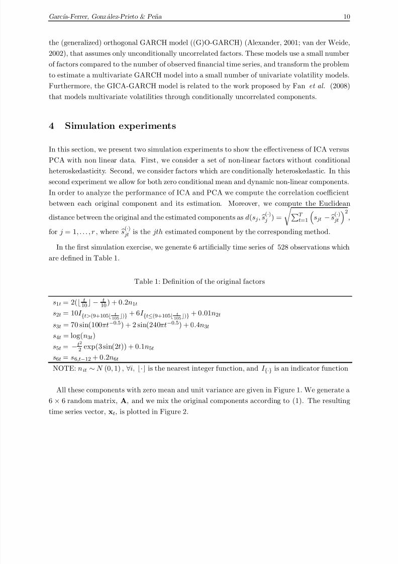
4 Simulation experiments

In this section, we present two simulation experiments to show the effectiveness of ICA versus

PCA with non linear data. First, we consider a set of non-linear factors without conditional

heteroskedasticity. Second, we consider factors which are conditionally heteroskedastic. In this

second experiment we allow for both zero conditional mean and dynamic non-linear components.

In order to analyze the performance of ICA and PCA we compute the correlation coefficient

between each original component and its estimation. Moreover, we compute the Euclidean

distance between the original and the estimated components as d(s j, s(·) j ) =

T t=1

s jt − s(·)

jt

2,

for j = 1, . . . , r , where s(·) jt is the jth estimated component by the corresponding method.

In the first simulation exercise, we generate 6 artificially time series of 528 observations which

are defined in Table 1.

Table 1: Definition of the original factors

s1t = 2( t10 − t

10 ) + 0.2n1t

s2t = 10I t>(9+105 t105) + 6I t≤(9+105 t105) + 0.01n2t

s3t = 70 sin(100πt−0.5) + 2 sin(240πt−0.5) + 0.4n3t

s4t = log(n3t)

s5t = −t2

2 exp(3 sin(2t)) + 0.1n5t

s6t = s6,t−12 + 0.2n6t

NOTE: nit ∼ N (0, 1) , ∀i, · is the nearest integer function, and I · is an indicator function

All these components with zero mean and unit variance are given in Figure 1. We generate a

6 × 6 random matrix, A, and we mix the original components according to (1). The resulting

time series vector, xt, is plotted in Figure 2.




−2

−1

0

−1

0

1

−4

−20

2

−4

−2

0

0 50 100 150 200 250 300 350 400 450 500

−1

0

1

−1

0

1

Figure 1: Original unobserved components

−40

−20

0

20

−40

−20

0

20

−40

−200

20

−40−20

020

0 50 100 150 200 250 300 350 400 450 500

−40

−20

0

20

−20

0

20

Figure 2: Observed data

We apply ICA and PCA to compute the estimates

A and

s

(·)t . Figures 3 shows

s

(·)t obtained

in the four estimation methods and in the same order as the original ones. We conclude that

ICA seems to perform better than PCA to estimate the non-linear factors.

−2

0

2

−2

0

2

0

2

4

−2

0

2

0 50 100 150 200 250 300 350 400 450 500

−2

0

2

−3−2−1

01

(a) sP t : Estimated factors obtained by PCA

−3

−2

−1

0

−1

0

1

−4

−2

0

2

−4

−2

0

0 50 100 150 200 250 300 350 400 450 500

−1

0

1

−1

0

1

2

(b) sF t : Estimated factors obtained by FastICA

−3

−2

−1

0

−1

0

1

−4

−2

0

2

−4

−2

0

0 50 100 150 200 250 300 350 400 450 500

−1

0

1

−2

0

2

(c) sJ t : Estimated factors obtained by JADE

−3

−2

−1

0

−1

0

1

−4

−2

0

2

−4

−2

0

0 50 100 150 200 250 300 350 400 450 500

−1

0

1

−2

0

2

(d) sSt :Estimated factors obtained by SOBI

Figure 3: Estimated factors using different procedures

In order to validate this intuition, Table 2 presents the correlation between the estimated and

generated components and we found that the correlations coefficients are higher for the ICs.

Furthermore, the Euclidean distance between the original components and the ICs is smaller




than the one corresponding to PCs (see Table 3). Then, we conclude that ICA performs better

than PCA to separate non-linear factors without heteroskedasticity. All ICA algorithms have a

similar performance.

Table 2: Correlation coefficient between

the original and the estimated components

FAST JADE SOBI PCA

1st 0.996 0.998 0.997 0.733

2nd 0.999 0.999 0.989 0.687

3rd 0.994 0.965 0.998 0.576

4th 0.991 0.993 0.991 0.834

5th 0.989 0.995 0.986 0.862

6th 0.994 0.988 0.998 0.653

Average 0.994 0.990 0.994 0.724

Table 3: Euclidean distance between the

original and the estimated components

FAST JADE SOBI PCA

1st 1.991 1.519 1.664 16.782

2nd 0.886 0.628 3.416 18.160

3rd 2.510 6.090 1.345 21.131

4th 3.095 2.640 3.125 13.230

5th 3.454 2.404 3.896 12.072

6th 2.523 3.531 1.589 19.130

Average 2.410 2.802 2.506 16.751

In the first part of the second experiment, we generate components which have constant

conditional mean but they are conditionally heteroskedastic. We generate six components of 1000

observations: three of them are gaussian random noises, and the other three are conditionally

heteroskedastic processes defined in Table 4.

Table 4: Definition of the original factors

s1t =√

h1tε1t; where h1t = 0.2 + 0.7s21t−1,

s2t = √ h2tε2t; where h2t = 0.021 + 0.073s22t−1 + 0.906h2t−1,

s3t =√

h3tε3t; where h3t = 1.692 + 0.245s23t−1 + 0.337h3t−1 + 0.310h3t−2,

NOTE: ε jt is a random noise with zero-mean and unit variance, and it is independent of h jt , ∀ j = 1, 2, 3

We standardize the components to satisfy the requirements of ICA, and we plot them in

Figure 4. Next, we generate a 6 × 6 random matrix, A, and we compute xt (see Figure 5)

according to (1) .

−4

−20

2

−4

−2

0

2

−2

0

2

−2

0

2

0 100 200 300 400 500 600 700 800 900 1000

−2

0

2

−8

−6−4−2

024


−8−6−4−2

024

−4−2

024

−10

−5

0

5

−4

−2

0

2

0 100 200 300 400 500 600 700 800 900 1000

−5

0

5

−2

0

2


We apply ICA and PCA to estimate the components, and compute the correlation coefficient

and the Euclidean distances between s jt and s(·)

jt , for j = 1, . . . , 6. Looking at the results, which




are shown in Tables 5 and 6 respectively, we conclude that the fitting of the ICs to the original

components is better than the one corresponding to PCA. However, in this case SOBI performs

worse than FastICA and JADE. This is to be expected as heteroskedastic processes have excess

kurtosis and small autocorrelation coefficients.

Table 5: Correlation coefficient betweenthe original and the estimated components

FAST JADE SOBI PCA

1st 0.985 0.995 0.907 0.778

2nd 0.993 0.992 0.747 0.750

3rd 0.934 0.928 0.838 0.708

4th 0.821 0.942 0.753 0.707

5th 0.869 0.909 0.637 0.530

6th 0.715 0.847 0.624 0.623

Average 0.886 0.934 0.751 0.683

Table 6: Euclidean distance between theoriginal and the estimated components

FAST JADE SOBI PCA

1st 5.521 5.505 13.637 21.056

2nd 3.777 4.080 22.476 22.358

3rd 11.484 12.004 18.015 24.175

4th 18.920 10.736 22.210 24.181

5th 16.214 13.500 26.950 30.630

6th 23.872 17.472 27.410 27.450

Average 13.298 10.549 21.783 24.975

In the second part of this experiment we make a mixture of the previous st and st and have

components that are both non-linear and conditionally heteroskedastic. We consider six time

series of 1000 observations. Three of them are zero-mean and unit variance random noises, and

the others are generated as:

s1t = s2t + s1t s2t = s3t + s3t s3t = s6t + s2t

where s jt , for j = 2, 3, 6, is defined in Table 1, and sit, for i = 1, 2, 3, is defined in Table 2.

The standardized components and the observed data set given by (1) , where A is randomlygenerated, are shown in Figures 6 and 7.

−1

0

1

−2

0

2

−2

0

2

−2

0

2

0 100 200 300 400 500 600 700 800 900 1000

−2

0

2

−4

−2

0

2


−5

0

5

−10

−5

0

5

−5

0

5

−4−2

02

0 100 200 300 400 500 600 700 800 900 1000

−4−2

024

−4

−2

0

2


Figure 8 shows the estimated components by ICA and PCA, and again ICA performs better

than PCA, specially for the non-noisy components.

Since the components are now heteroskedastic and also have a non-linear conditional mean,

SOBI performs as well as, or even better than, FastICA and JADE. The correlation coefficients

(Table 7) and the Euclidean distances (Table 8) between the original and the estimated compo-

nents, confirm our visual results. In fact, according to the average results, SOBI has the best

performance for non-linear and conditionally heteroskedastic components.




−2

0

2

−2

0

2

−2

0

2

−2

0

2

0 100 200 300 400 500 600 700 800 900 1000

−2

0

2

−2

0

2

(a) sP t : Estimated factors obtained by PCA

−1

0

1

2

−2

0

2

−2

0

2

−2

0

2

0 100 200 300 400 500 600 700 800 900 1000

−2

0

2

−4

−2

0

2

(b) sF t : Estimated factors obtained by FastICA

−1

0

1

−2

0

2

−2

0

2

−2

0

2

0 100 200 300 400 500 600 700 800 900 1000

−2

0

2

−4

−2

0

2

(c) sJ t : Estimated factors obtained by JADE

−1

0

1

−2

0

2

−2

0

2

−2

0

2

0 100 200 300 400 500 600 700 800 900 1000

−2

0

2

−4

−2

0

2

(d) sSt : Estimated factors obtained by SOBI

Figure 8: Estimated unobserved components using different procedures

Table 7: Correlation coefficient between

the original and the estimated components

FAST JADE SOBI PCA

1st 0.988 0.996 0.998 0.602

2nd 0.991 0.998 0.999 0.536

3rd 0.966 0.983 0.990 0.650

4th 0.931 0.633 0.871 0.447

5th 0.827 0.731 0.965 0.626

6th 0.746 0.755 0.827 0.737

Average 0.908 0.849 0.942 0.600

Table 8: Euclidean distance between the

original and the estimated components

FAST JADE SOBI PCA

1st 4.839 2.812 1.771 28.197

2nd 4.238 2.151 0.995 30.457

3rd 8.222 5.788 4.530 26.446

4th 11.779 27.098 16.035 33.227

5th 18.586 23.210 8.313 27.343

6th 22.543 22.122 18.611 22.937

Average 11.701 13.863 8.376 28.101

From these simulations, we conclude that, under non-gaussian data, ICA recovers the com-

ponents better than PCA. The performance of the three ICA algorithms is as expected: SOBI

is better than JADE or FastICA if the components have dynamics in the mean, both when the

components are heteroskedastic and when they are not. Furthermore, when the components are

conditionally heteroskedastic with constant conditional mean JADE and FastICA perform well,

whereas SOBI is similar to PCA. This is not a surprising result because the SOBI components

are the rotation of the PCs that diagonalize a set of time delayed covariance matrices, and the




conditionally heteroskedastic components are not time dependent.

5 Empirical application

In this section we apply our procedure to a real dataset of stock returns. First, we describe thedata used; second, we explain the procedure to estimate the components; and third, we present

the results of using ICs and PCs to forecast the volatility of the stock returns.

We use daily closing prices from the Madrid stock market. The data are from the 19 assets

which were always included in the IBEX 35 from 2000 to 20041. The IBEX 35 index is the

main stock market index of the Bolsa de Madrid. Its composition is revised twice a year and

it comprises the 35 companies with the largest trading volume of the Madrid stock exchange.

We apply some preprocessing steps to the data. First of all, we transform daily closing prices

to daily stock returns to achieve stationarity. The daily stock returns of the ith company are

computed as:

rit = log ( pit+1) − log ( pit) , i = 1,..., 19, (23)

where pit is the daily closing price of the ith asset at time t. Then, we have a 19 × 1250

multivariate vector of stock returns, which is denoted by rt, whose columns are the value of

these 19 stocks in the 1250 trading days in the period 2000-2004. There are some extreme

observations that correspond to outliers, which are due to well know changes, such as stock

splits or other legal changes. Finally, after the outliers have been removed, we also remove the

mean from the stocks returns, xt = rt − E [rt], and these 19 preprocessed daily stock returnstime series are shown in Figure 9.

0 200 400 600 800 1000 1200−0.2

−0.1

0

0.1

0.2

Figure 9: Series of daily stock returns from 2000 to 2004 (without outliers)

We compute the kurtosis coefficients of xt and the results are displayed in Table 9. The

distribution of daily stock returns is leptokurtic, that is, they are far away from gaussianity.

1The 19 stocks are listed in the Appendix.




Table 9: Kurtosis coefficients of the transformed daily stock returns

ACS ACX ALT AMS ANA BBVA BKT ELE

5.3619 4.8558 5.9571 5.3303 5.8949 4.7493 5.9641 5.4053

FCC FER IBE IDR NHH POP REP SAN

5.0625 4.6196 5.3139 4.8257 4.776 4.9358 4.9307 5.0546SGC TEF TPI

4.8686 4.0998 5.5625

The 19 unobserved factors are estimated using both PCA and ICA and they are sorted in

terms of the explained total variance. The results are displayed in Table 10.

Table 10: Sorted components in terms of their explained variability

PCA %PCA FAST %Fast JADE %JADE SOBI %SOBI

sP 1t 35.30 sF 1t 17.72 sJ 1t 11.75 sS1t 11.13 sP 2t 7.00 sF 2t 10.22 sJ 2t 7.29 sS2t 9.65

sP 3t 5.91 sF 3t 6.40 sJ 3t 6.48 sS3t 9.16

sP 4t 4.78 sF 4t 5.92 sJ 4t 6.36 sS4t 8.15

sP 5t 4.73 sF 5t 5.76 sJ 5t 6.17 sS5t 7.52

sP 6t 4.35 sF 6t 4.89 sJ 6t 5.70 sS6t 5.42

sP 7t 4.24 sF 7t 4.65 sJ 7t 5.61 sS7t 5.23

sP 8t 4.04 sF 8t 4.62 sJ 8t 5.52 sS8t 4.37

sP 9t 3.62 sF 9t 4.43 sJ 9t 5.20 sS9t 4.11

sP 10t 3.60 sF 10t 4.15 sJ 10t 5.16 sS10t 4.00

sP 11t 3.31 sF 11t 3.86 sJ 11t 5.12 sS11t 3.83

sP 12t 3.13 sF 12t 3.85 sJ 12t 4.74 sS12t 3.73

sP 13t 3.03 sF 13t 3.69 sJ 13t 4.01 sS13t 3.57

sP 14t 2.86 sF 14t 3.67 sJ 14t 3.85 sS14t 3.57 sP 15t 2.66 sF 15t 3.56 sJ 15t 3.84 sS15t 3.57

sP 16t 2.56 sF 16t 3.47 sJ 16t 3.76 sS16t 3.42

sP 17t 2.21 sF 17t 3.26 sJ 17t 3.51 sS17t 3.26

sP 18t 1.71 sF 18t 2.97 sJ 18t 3.41 sS18t 3.22

sP 19t 0.93 sF 19t 2.89 sJ 19t 2.51 sS19t 3.10

1.00 1.00 1.00 1.00

We use Figure 10, that shows the explained variability by the components estimated by the

four algorithms, to decide the optimal number of components for each method. The results

are given in Table 11, that also includes the absolute explained variability by the r selected

components.

Table 11: Number of unobserved components and percentage of total explained variability

PCA FAST JADE SOBI

r 1 2 2 5

% variability 35.30 27.95 19.04 45.62

We are interested in investigating which assets are more important to define each component.

From (2) , sit19i=1 can be written as a linear combination of the stock returns, sit = 19

j=1 wijx jt ,where wij represents the effect of the jth stock returns on the ith component, and the largest

weights correspond to the most important assets. The ICs and the PCs have different interpre-

tation. For example, if we focus on the first component, we have that, on one hand, the first PC




5 10 150

10

20

30

40

5 10 150

5

10

15

20

5 10 150

5

10

15

5 10 150

5

10

15

SOBIJADE

FastICAPCA

Figure 10: Explained total variability by the components.

can be seen as a weighted mean of the 19 daily stock returns time series, it is an index of the

market. Indeed, if we plot the variation of variability of the first PC and the IBEX 35 index,

considering groups of ten observations, it is clear that the first PC reflects the main movements

of the index IBEX 35 (see Figure 11). Then, if we forecast the volatility of xt from the volatility

of the first PC, the 19 stock returns will tend to move together.

0 20 40 60 80 100 120−4

−3

−2

−1

0

1

2

3

4

5

PCA

IBEX 35

Figure 11: Variation of variability of

sP 1t and the IBEX 35 index

On the other hand, the first ICs cannot be seen as indexes of the market. They are mainlyassociated with electricity, building industries, and banking2, and separate the stock returns in

terms of the individual explained variability, ν i119i=1 (see (15)). As an example, we analyze the

first FastICA, sF 1t. In Figure 12, that shows the variation of variability of sF

1t and the largest

weighted assets on sF 1t, we see that all assets present a cluster of high variability from observation

600 to 750. The assets which are positively weighted only have this period of higher variability,

but the negative ones are also volatile at the beginning of the sample.

The forecasting performance of our model is checked as follows:

1. We estimate A and the unobserved components, by ICA and PCA, using the whole sample.

Then, the components are sorted and r is fixed.

2The sectorial economic classification is detailed in the Appendix.




0 50 100−10

0

10

0 50 100−10

0

10

0 50 100−10

0

10

0 50 100−10

0

10

0 50 100−10

0

10

0 50 100−10

0

10

ELE

FAST1

BBVA

FAST1

POP

FAST1

FCC

FAST1

ANA

FAST1

IBE

FAST1

Figure 12: Variation of variability of

sF 1t

and the stock returns with the largest weights: a) on the left,

the positive ones; b) on the right, the negative ones.

2. Using the whole sample, we fit an ARMA( p, q ) with GARCH ( p, q ) disturbances for each

component s jt , with j = 1,...,r.

3. We estimate the parameters of the ARMA( p, q )-GARCH ( p, q ) model with a sample of

1000 observations. Then, we generate the one-step-ahead forecast for the volatility of each s jt,

h j,1001|1000 = V [

s j1001|I1000] , j = 1,...,r. (24)

Thus, by rolling prediction for t

= 1001, ...,

1250, we have: Ht|1000 = diag( h1,t|1000, ..., hr,t|1000), t = 1001, ..., 1250, (25)

which is the conditional covariance matrix of st = ( s1t, ..., srt) at time t.

4. According to (20), we compute the conditional variance of xt at time t, Ωt, and the

conditional variance of xi at time t is given by the ith diagonal term of Ωt,

γ 2i,t|1000 =

r j=1

h j,t|1000a2ij, i = 1, 2, ..., 19, t = 1001, ..., 1250. (26)

Then, we forecast the conditional variance of the stock returns from the predicted volatility

of the unobserved components.

5. To evaluate the forecasting performance of GICA-GARCH and O-GARCH models, we

need to compare the predicted volatility with respect to the real one. However, volatility

cannot be observed. Following Franses and van Dijk (1996), we measure the ‘true volatility’

of the ith stock return at time t by:

υit = (xit − xi)2 , i = 1,..., 19, t = 1001, ..., 1250, (27)

where xi is the average return of xi over the last 1000 observations. Then, the one-step-

ahead forecast error is given by:

it = υit − γ 2i,t|1000, i = 1, 2,..., 19, t = 1001, ..., 1250. (28)




6. To evaluate the accuracy of the model we divide the prediction error (28) by some al-

ternative benchmark. This benchmark is obtained using another standard method of

forecasting. Let us assume that the benchmark method predicts the volatility of the stock

returns by their marginal variance. Then, we define the relative ratio as:

RE it = it

∗it

, i = 1, 2, ..., 19, t = 1001,..., 1250, (29)

where ∗it is the forecast error of the ith stock return obtained by the benchmark method.

That is,

∗it = υit − σ2i , i = 1, 2, ..., 19, t = 1001,..., 1250. (30)

where σ2i is the marginal variance of the ith stock return at time t. To minimize the impact

of outliers when we analyze the volatility forecasting performance of GICA-GARCH and

O-GARCH models, we use the Median Relative Absolute Error (MdRAE) criteria3:

MdRAE (RE it) = median(|RE it|)

Instead of using relative errors, we can use the relative measures by computing the ratio

of the corresponding measure for the ICA method to respect the PCA one:

RelMdRAE = MdRAE IC A

MdRAE P CA(31)

In order to analyze the effect of increasing the number of components, we vary r from 1 to

5 to evaluate the forecasting performance of the model. The results are displayed in Table 12.

For each forecast model, this table shows the mean average of the RelMdRAE measured over

the 19 stock returns.

Table 12: Mean average of the RelMdRAE measured over the 19 stock returns

Number of Components (r) FAST JADE SOBI PCA

1 0.767 0.774 0.741 1

2 0.824 0.800 0.760 1

3 0.743 0.711 0.686 1

4 0.708 0.667 0.678 1

5 0.735 0.708 0.690 1

From Table 12, we conclude that the forecasting performance of GICA-GARCH model is

better than the corresponding to O-GARCH one, independently of the ICA algorithms we use

and of the number of factors we consider. SOBI gives the best forecasting overall results except

when r = 4. However, note that for r = 4 the differences between JADE and SOBI are not

significant. Results are specially surprising when r = 1. Remember that PCA considers only

one component as the optimal number of factors, and its explained variability is higher than the

corresponding to the first ICs. One would expect that, when r = 1, PCA would show the best

forecasting performance, but this is not so: any of the ICA algorithms performs better than

PCA. Note that because we are dealing with relative ratios, we cannot say anything about the

performance of each algorithm when the number of factors increases.

3See Hyndman and Koehler (2006) for a complete revision of measures of forecast accuracy.




Evaluating the forecasting performance of the model using the Relative Geometric Mean

Relative Absolute Error (RelGMRAE ) gives similar results which are available from the authors

upon request.

6 Concluding remarks

We have proposed a new framework for modelling multivariate volatilities. We have introduced

the GICA-GARCH model that can be seen as an extension of the orthogonal factor GARCH

models. The GICA-GARCH model assumes that the comovements of a vector of financial data

are driven a few independent components which are estimated by ICA. The GICA-GARCH

model allows to estimate a multivariate GARCH model using a small number of independent

and conditionally heteroskedastic factors, which evolve according to univariate GARCH models.

Then, our model gives a parsimonious representation of the data, and reduces the number of

parameters to be estimated. Interestingly, the GICA-GARCH model can also be seen as a

particular dynamic factor GARCH model. Note, however, that while in the dynamic factor

GARCH model the covariance matrix of the noise is of full rank, the GICA-GARCH will have

rank equal to m − r . Nevertheless, this assumption can be relaxed easily by assuming an

additional measurement noise so that the covariance matrix is of full rank.

In this paper, we have used three ICA algorithms for estimating the ICs. Their performance

have been tested on some simulation experiments, and we conclude that in all cases ICA methods

performs better than PCA to estimate non-linear and/or heteroskedastic components. However,

the results among the different ICA algorithms are mixed. For non-linear factors (conditionally

heteroskedastic or not), all work well but when the factors are conditionally heteroskedastic anddo not have dynamics in the mean, SOBI performs worse than both JADE and FastICA.

The GICA-GARCH seems to work better for forecasting the volatility of the financial stock

returns than the O-GARCH model.

In the future, we intend to design an alternative procedure to sort the ICs and to choose

the optimal number of factors. Also, comparing the forecasting performance of our model with

other multivariate GARCH and extending the GICA-GARCH model to other applications, may

be challenges for the future.

References

Alessi, L., Barigozzi, M., and Capasso, M. (2006). Dynamic factor GARCH: Multivariate

volatility forecast for a large number of series . LEM Papers Series 2006/25. Laboratory of

Economics and Management (LEM). Sant’Anna School of Advanced Studies. Pisa, Italy.

Alexander, C. (2001). Market Models: A guide to financial data analysis . Chichester, U.K.:

Wiley.

Back, A. D. and Weigend, A. S. (1997). A first application of independent component analysis

to extracting structure from stock returns. International Journal of Neural Systems 8, 473-484.

Bauwens, L., Laurent, S., and Rombouts, J. V. K. (2006). Multivariate GARCH models: a

survey. Journal of Applied Econometrics 21, 79-109.




Belouchrani, A., Abed Meraim, K., Cardoso, J.-F., and Moulines, E. (1997). A blind source

separation tecnique based on second order statistics. IEEE Transactions on Signal Processing

45, 434-444.

Bollerslev, T. (1986). Generalized autoregressive conditional heteroscedasticity. Journal of

Econometrics 31, 307-327.

Bollerslev, T., Engle, R. F., and Wooldridge, J. W. (1988). A capital asset pricing model with

time-varying covariances. Journal of Political Economy 96, 116-131.

Cardoso, J.-F. and Souloumiac, A. (1993). Blind beamforming for non-gaussian signals. IEE-

Proceedings-F 140, 362-370.

Cha, S.-M. and Chan, L.-W. (2000). Applying independent component analysis to factor

model in finance. IDEAL, 538-544.

Comon, P. (1994). Independent component analysis - a new concept?. Signal Processing 36,

287-314.

Diebold, F. X. and Nerlove, M. (1989). The dynamics of exchange rate volatility: a multi-

variate latent factor ARCH model. Journal of Applied Econometrics 4, 1–21.

Engel, R. F. (1982). Autoregressive conditional heteroscedasticity with estimates of the vari-

ance of United Kingdom inflation. Econometrica 50, 987-1007.

Fan, J., Wang, M., and Yao, Q. (2008). Modelling multivariate volatilities via condition-

ally uncorrelated components. Journal of The Royal Statistical Society: Series B (Statistical

Methodology) 70(4), 679-702.

Franses, Ph. H. and van Dijk, D. (1996). Forecasting stock market volatility using nonlinear

GARCH models. Journal of Forecasting 15, 229-235.

Hyndman, R. J. and Koehler, A. B. (2006). Another look at measures of forecast accuracy.

International Journal of Forecasting 22, 679-688.

Hyvarinen, A. (1999). Fast and robust fixed-point algorithms for independent component

analysis. IEEE. Transaction on Neural Networks 10, 626-634.

Hyvarinen, A. and Kano, K. (2003). Independent component analysis for non-normal factor

analysis. In H. Yanai et al. (Ed.) New Developments in Psychometrics , pp. 649-656. Tokyo:

Springer Verlag.

Hyvarinen, A., Karhunen, J., and Oja, E. (2001). Independent component analysis . New

York: Wiley.

Hyvarinen, A. and Oja, E. (1997). A fast fixed-point algorithm for independent component

analysis. Neural Computation 9, 1483-1492.

Kiviluoto, K., and Oja, E. (1998). Independent component analysis for parallel financial time

series. In Proc. Int. Conf. on Neural Information Processing , vol. 2, pp. 895-898. Tokyo.

Lanne, M. and Saikkonen, P. (2007). A multivariate generalized orthogonal factor GARCH

model. Journal of Business and Economic Statistics 25, 61-75.

Malaroiu, S., Kiviluoto, K., and Oja, E. (2000). Time series prediction with independent




component analysis. Technical Report . Helsinki University of Technology. Helsinki.

Pena, D. and Box, G. (1987). Identify a simplifying structure in time series. Journal of The

American Statistical Association 82, 836-843.

Stock, J. H. and Watson, M. W. (2002). Macroeconomic forecasting using diffusion indexes.

Journal of Business and Economic Statistics 20, 147-162.Tong, L., Liu, R.-W., Soon, V. C., Huang, Y.-F., and Liu, R. (1990). AMUSE: A new blind

identification algorithm. Proceedings of IEEE ISCAS .

van der Weide, R. (2002). GO-GARCH: a multivariate generalized orthogonal GARCH model.

Journal of Applied Econometrics 17, 549-564.

Wu, E. H. C. and Yu, P. L. H. (2005). Volatility modelling of multivariate financial time

series by using ICA-GARCH models. IDEAL, 571-579.

AppendixComponents of the IBEX 35 from 2000 to 2004 classified by sectors

Consumption

Other goods of consumption ALT Altadis

Consumption services

Leisure time / Tourism / Hotel industry AMS Amadeus

NHH NH Hoteles

Mass media / Publicity SGC Sogecable

TPI Telefonica Publicidad e Informacion

Financial Services / Estate Agencies

Banking BBVA Banco Bilbao Vizcaya Argentaria

BKT BankinterPOP Banco Popular

SAN Banco Santander Central Hispano(∗)

Oil and Energy

Oil REP Repsol

Electricity and Gas ELE Endesa

IBE Iberdrola

Materials / Industry / Building

Minerals / Metals ACX Acerinos

Building ACS Grupo ACS

ANA Acciona

FCC Fomento de Construcciones y Contratas S.A.

FER Grupo Ferrovial

Technology / TelecommunicationsTelecommunications and others TEF Telefonica

Electronic and Software TPI Indra(∗)From 01/01/2000 to 31/10/2001, its name was SCH.




Univariate GARCH models: Specification chosen for the components in the four estima-

tion methods.

PCA FastICA

sP 1t ∼ GARCH (1, 1) sF 1t ∼ GARCH (1, 1)

sP 2t ∼ AR(1) + GARCH (1, 1) sF 2t ∼ AR(2) + GARCH (1, 1)

sP 3t ∼ AR(1) + GARCH (1, 1) sF

3t ∼ GARCH (1, 1)

sP 4t ∼ AR(2) + ARCH (1) sF 4t ∼ GARCH (2, 2)

sP 5t ∼ GARCH (1, 1) sF 5t ∼ AR(1) + GARCH (1, 1)

JADE SOBI

sJ 1t ∼ GARCH (1, 1) sS1t ∼ M A(1) + GARCH (1, 1)

sJ 2t ∼ ARCH (1, 1) sS2t ∼ ARMA(1, 1) + GARCH (1, 1)

sJ 3t ∼ ARMA(1, 1) + GARCH (1, 1) sS3t ∼ GARCH (1, 1)

sJ 4t ∼ GARCH (1, 1) sS4t ∼ M A(1) + GARCH (1, 1)

sJ 5t ∼ GARCH (1, 1) sS5t ∼ AR(1) + GARCH (1, 1)

a multivariate generalized independent factor garch model with an application to financial stock...

Documents