multivariate garch models -...
TRANSCRIPT

Multivariate GARCH Models
Eduardo Rossi
University of Pavia

Introduction
Economics and financial economics present problems whose solutions
need the specification and estimation of a multivariate distribution.
• the standard portfolio allocation problem
• the risk management of a portfolio of assets
• pricing of derivative contracts based on a more than one
underlying asset (e.g., Quanto options)
• Financial contagion (shocks transmission volatility and returns)
Eduardo Rossi c© - Econometria finanziaria 2010 2

Introduction
Stylized facts:
• Volatility clustering
• Time-varying dynamic covariances and dynamic correlations
Financial variables have time-dependent second order moments.
Parametric models:
1. Multivariate GARCH models
2. Multivariate Stochastic volatility models
3. Multifactor models
4. Multifactor realized volatility models
Eduardo Rossi c© - Econometria finanziaria 2010 3

Multivariate Volatility Models
Vector of returns:
yt = (y1t, . . . , yNt)′ (N × 1)
yt − µt = ǫt = H−1/2t zt
Let {zt} be a sequence of (N × 1) i.i.d. random vector with the
following characteristics:
E [zt] = 0
E [ztz′
t] = IN
zt ∼ G (0, IN )
with G continuous density function.
Eduardo Rossi c© - Econometria finanziaria 2010 4

Multivariate Volatility Models
Et−1 (ǫt) = 0
Et−1 (ǫtǫ′
t) = Ht
E (ǫtǫ′
t) = Σ
Et−1[·] = E[·|Φt−1]
Φt−1 is the σ-field generated by past values of observable variables.
where Ht is a matrix (N ×N) positive definite and measurable with
respect to the information set Φt−1, that is the σ-field generated by
the past observations: {ǫt−1, ǫt−2, . . .}.The correlation matrix:
Corrt−1(ǫt) = Rt = D−1/2t HtD
−1/2t
Dt = diag(h11,t, . . . , hNN,t)
Eduardo Rossi c© - Econometria finanziaria 2010 5
Multivariate Volatility Models
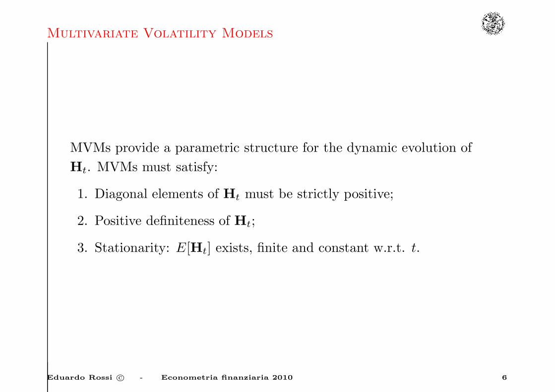
MVMs provide a parametric structure for the dynamic evolution of
Ht. MVMs must satisfy:
1. Diagonal elements of Ht must be strictly positive;
2. Positive definiteness of Ht;
3. Stationarity: E[Ht] exists, finite and constant w.r.t. t.
Eduardo Rossi c© - Econometria finanziaria 2010 6

Multivariate Volatility Models
Ideal characteristics of a MVM:
1. Estimation should be flexible for increasing N
2. It should allow for covariance spillovers and feedbacks;
3. Coefficients should have an economic or financial interpretation
Eduardo Rossi c© - Econometria finanziaria 2010 7

MGARCH
The extension from a univariate GARCH model to an N -variate
model requires allowing the conditional variance-covariance matrix of
the N -dimensional zero mean random variables ǫt depend on the
elements of the information set.
Eduardo Rossi c© - Econometria finanziaria 2010 8
Covariance targeting
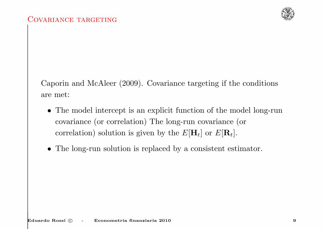
Caporin and McAleer (2009). Covariance targeting if the conditions
are met:
• The model intercept is an explicit function of the model long-run
covariance (or correlation) The long-run covariance (or
correlation) solution is given by the E[Ht] or E[Rt].
• The long-run solution is replaced by a consistent estimator.
Eduardo Rossi c© - Econometria finanziaria 2010 9
Covariance targeting: example
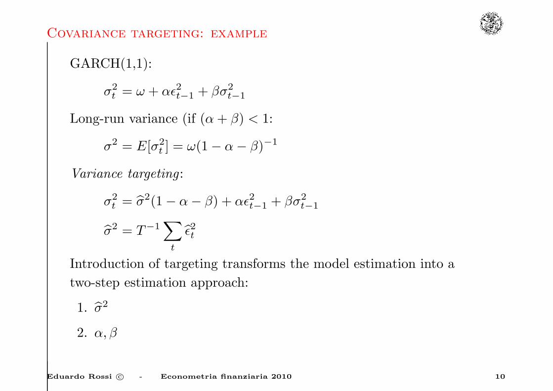
GARCH(1,1):
σ2t = ω + αǫ2t−1 + βσ2
t−1
Long-run variance (if (α+ β) < 1:
σ2 = E[σ2t ] = ω(1− α− β)−1
Variance targeting :
σ2t = σ2(1− α− β) + αǫ2t−1 + βσ2
t−1
σ2 = T−1∑
t
ǫ2t
Introduction of targeting transforms the model estimation into a
two-step estimation approach:
1. σ2
2. α, β
Eduardo Rossi c© - Econometria finanziaria 2010 10

Covariance targeting: example
N assets: N variances + 12N(N − 1) covariances = N
2 (N + 1).
Two alternative approaches:
• Models of Ht
• Models of Dt and Rt
The parametrization of Ht as a multivariate GARCH, which means
as a function of the information set Φt−1, allows each element of Ht
to depend on q lagged of the squares and cross-products of ǫt, as well
as p lagged values of the elements of Ht. So the elements of the
covariance matrix follow a vector of ARMA process in squares and
cross-products of the disturbances.
Eduardo Rossi c© - Econometria finanziaria 2010 11

MGARCH-Vech representation
Let vech denote the vector-half operator, which stacks the lower
triangular elements of an N ×N matrix as an [N (N + 1) /2]× 1
vector.
Let A be (2× 2), then vech(A)
vech(A) =
a11
a21
a22
Since the conditional covariance matrix Ht is symmetric,
vech (Ht) , (N(N + 1)/2× 1) contains all the unique elements in Ht.
Eduardo Rossi c© - Econometria finanziaria 2010 12

MGARCH-Vech representation
A natural multivariate extension of the univariate GARCH(p,q)
model is
vech (Ht) = W +
q∑
i=1
A∗
i vech(ǫt−iǫ
′
t−i
)+
p∑
j=1
B∗
jvech (Ht−j)
= W +A∗ (L) vech (ǫtǫ′
t) +B∗ (L) vech (Ht)
A∗ (L) = A∗
1L+ . . .+A∗
qLq
B∗ (L) = B∗
1L+ . . .+B∗
qLp
Eduardo Rossi c© - Econometria finanziaria 2010 13

MGARCH-Vech representation
N∗ ≡ N(N + 1)
2
W : [N (N + 1) /2]× 1
A∗
i , B∗
j : [N∗ ×N∗]
N = 2, Vech-GARCH(1,1):
h11,t
h21,t
h22,t
=
w∗1
w∗2
w∗3
+
a∗11
a∗12
a∗13
a∗21
a∗22
a∗23
a∗31
a∗32
a∗33
ǫ21,t−1
ǫ1,t−1ǫ2,t−1
ǫ22,t−1
+
b∗11
b∗12
b∗13
b∗21
b∗22
b∗23
b∗31
b∗32
b∗33
h11,t−1
h21,t−1
h2,t−1
Eduardo Rossi c© - Econometria finanziaria 2010 14

MGARCH-Vech representation
• This general formulation is termed vec representation by Engle
and Kroner (1995).
• The number of parameters is[1 + (p+ q) [N (N + 1) /2]2
].
• Even for low dimensions of N and small values of p and q the
number of parameters is very large; for N = 5 and p = q = 1 the
unrestricted version of (1) contains 465 parameters.
• The number of parameters is of order O(N4): the curse of
dimensionality.
For any parametrization to be sensible, we require that Ht be
positive definite for all values of ǫt in the sample space in the vech
representation this restriction can be difficult to check, let alone
impose during estimation.
Eduardo Rossi c© - Econometria finanziaria 2010 15
MGARCH-Diagonal vech model
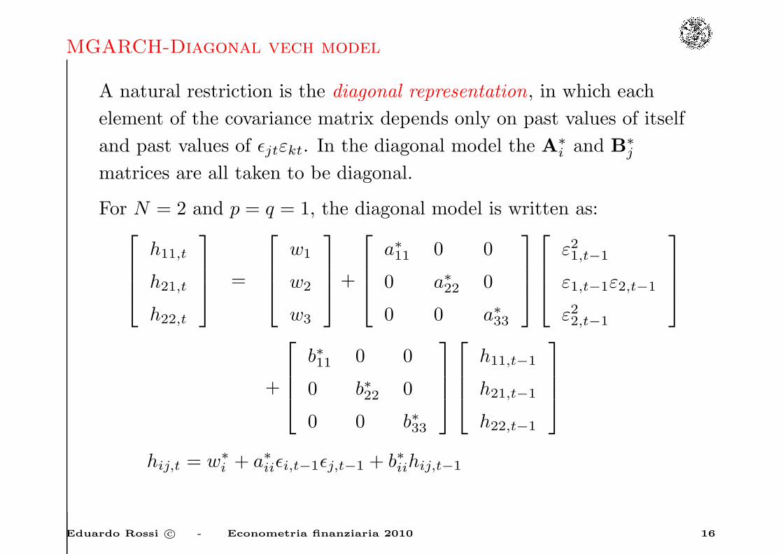
A natural restriction is the diagonal representation, in which each
element of the covariance matrix depends only on past values of itself
and past values of ǫjtεkt. In the diagonal model the A∗
i and B∗
j
matrices are all taken to be diagonal.
For N = 2 and p = q = 1, the diagonal model is written as:
h11,t
h21,t
h22,t
=
w1
w2
w3
+
a∗11 0 0
0 a∗22 0
0 0 a∗33
ε21,t−1
ε1,t−1ε2,t−1
ε22,t−1
+
b∗11 0 0
0 b∗22 0
0 0 b∗33
h11,t−1
h21,t−1
h22,t−1
hij,t = w∗
i + a∗iiǫi,t−1ǫj,t−1 + b∗iihij,t−1
Eduardo Rossi c© - Econometria finanziaria 2010 16

MGARCH-Diagonal vech model
Thus the (i, j) th element in Ht depends on the corresponding (i, j) th
element in εt−1ε′
t−1 and Ht−1. This restriction reduces the number of
parameters to [N (N + 1) /2] (1 + p+ q). This model does not allow
for causality in variance, co-persistence in variance and asymmetries.
The number of parameters is of order O(N2).
The diagonal vech is equivalent to:
Ht = W +A⊙ ǫt−1ǫ′
t−1 +B⊙Ht−1
where A and B are symmetric matrices. ⊙ is the Hadamard product.
Eduardo Rossi c© - Econometria finanziaria 2010 17

MGARCH(1,1)-vech-Unconditional Covariance Matrix
Given that
ǫtǫ′
t = Ht +Vt
with Et−1 (Vt) = 0.
vech (ǫtǫ′
t) = vech (Ht) + vech (Vt)
vech (Vt) vector m.d.s.
with E (vech (Vt)) = vech(E (Vt)) = 0.
Eduardo Rossi c© - Econometria finanziaria 2010 18

MGARCH(1,1)-vech-Unconditional Covariance Matrix
For a GARCH(1,1), the unconditional covariance matrix, when it
exists, is given by
vech (ǫtǫ′
t) = W +A∗
1vech(ǫt−1ǫ
′
t−1
)
+B∗
1
[vech
(ǫt−1ǫ
′
t−1
)− vech (Vt−1)
]+ vech (Vt)
E (ǫtǫ′
t) = Σ
vech (E (ǫtǫ′
t)) = W + (A∗
1 +B∗
1)[vech
(E(ǫt−1ǫ
′
t−1
))]
vech (Σ) = [IN∗ −A∗
1 −B∗
1]−1
W.
For a GARCH(p,q) model
vech (Σ) = [IN∗ −A∗ (1)−B∗ (1)]−1
W
Eduardo Rossi c© - Econometria finanziaria 2010 19

MGARCH-vech representation
Targeting cannot easily introduced in the model.
MGARCH(1,1)-vech, unconditional var-cov matrix
[IN∗ −A∗
1 −B∗
1]vech(Σ)
Σ = T−1∑
t
ǫtǫ′
t
Targeting allows reducing by N∗ the parameters to be estimated.
The total number of parameters is still O(N4).
vech (Ht) = vech(Σ)+A∗
1vech[ǫt−1ǫ
′
t−1 − vech(Σ)]
+B∗
1
[vech (Ht−1)− vech
(Σ)]
Eduardo Rossi c© - Econometria finanziaria 2010 20
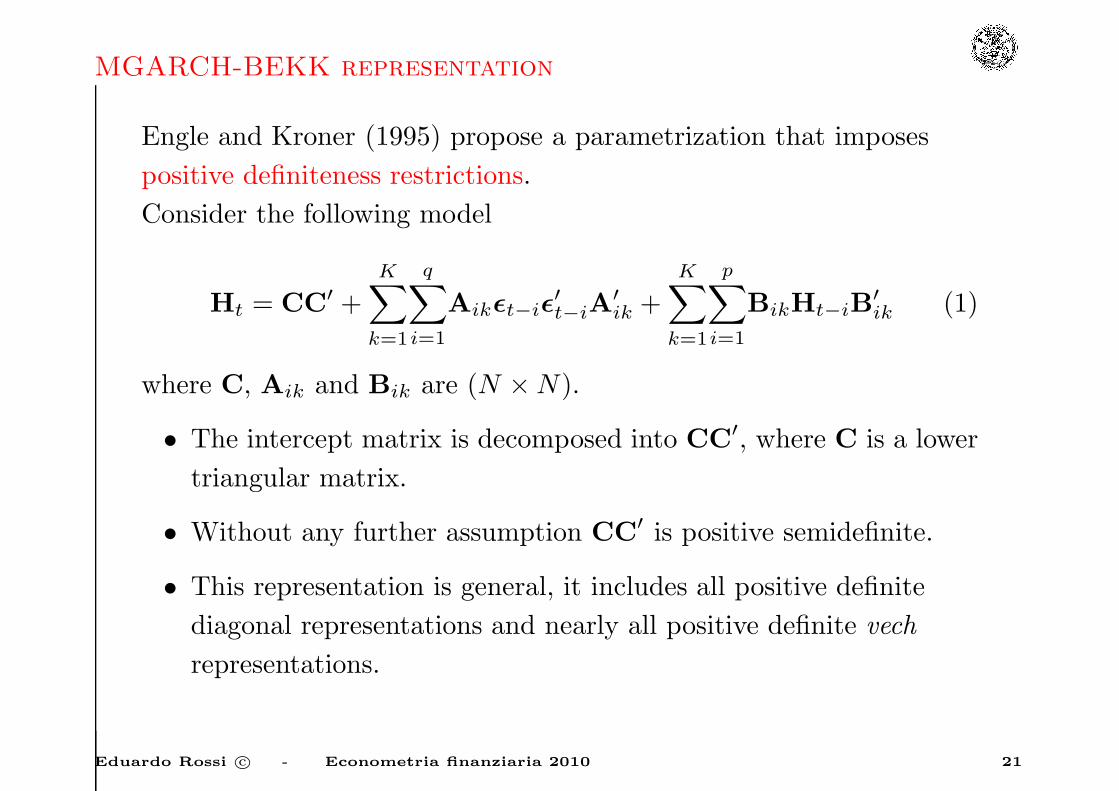
MGARCH-BEKK representation
Engle and Kroner (1995) propose a parametrization that imposes
positive definiteness restrictions.
Consider the following model
Ht = CC′ +K∑
k=1
q∑
i=1
Aikǫt−iǫ′
t−iA′
ik +K∑
k=1
p∑
i=1
BikHt−iB′
ik (1)
where C, Aik and Bik are (N ×N).
• The intercept matrix is decomposed into CC′, where C is a lower
triangular matrix.
• Without any further assumption CC′ is positive semidefinite.
• This representation is general, it includes all positive definite
diagonal representations and nearly all positive definite vech
representations.
Eduardo Rossi c© - Econometria finanziaria 2010 21

MGARCH-BEKK representation
For exposition simplicity we will assume that K = 1:
Ht = CC′ +
q∑
i=1
Aiǫt−iǫ′
t−iA′
i +
p∑
i=1
BiHt−iB′
i
Consider the simple GARCH(1,1) model:
Ht = CC′ +A1ǫt−1ǫ′
t−1A′
1 +B1Ht−1B′
1 (2)
Proposition 1. (Engle and Kroner (1995)) Suppose that the
diagonal elements in C are restricted to be positive and that a11 and
b11 are also restricted to be positive. Then if K = 1 there exists no
other C, A1, B1 in the model (2) that will give an equivalent
representation.
Eduardo Rossi c© - Econometria finanziaria 2010 22

MGARCH-BEKK representation
The purpose of the restrictions is to eliminate all other
observationally equivalent structures.
For example, as relates to the term A1ǫt−1ǫ′
t−1A′
1 the only other
observationally equivalent structure is obtained by replacing A1 by
−A1. The restriction that a11 (b11) be positive could be replaced
with the condition that aij (bij) be positive for a given i and j, as
this condition is also sufficient to eliminate −A1 from the set of
admissible structures.
Eduardo Rossi c© - Econometria finanziaria 2010 23

MGARCH-BEKK representation
MGARCH(1,1)-BEKK, N = 2:
Ht = CC′ +
a11 a12
a21 a22
ε21t−1 ε1t−1ε2t−1
ε2t−1ε1t−1 ε22t−1
a11 a12
a21 a22
′
+
b11 b12
b21 b22
h11t−1 h12t−1
h21t−1 h22t−1
b11 b12
b21 b22
′
Eduardo Rossi c© - Econometria finanziaria 2010 24

MGARCH-BEKK representation
Sufficient condition for positive definiteness of Ht in
BEKK-GARCH(p,q) model.
Proposition 2. (Engle and Kroner (1995)) (Sufficient condition)
If H0, H−1, . . . ,H−p+1 are all positive definite, then the BEKK
parametrization (with K = 1) yields a positive definite Ht for all
possible values of εt if C is a full rank matrix or if any Bi
i = 1, . . . , p is a full rank matrix.
Eduardo Rossi c© - Econometria finanziaria 2010 25

MGARCH-BEKK representation
For simplicity consider the GARCH(1,1) model. The BEKK
parameterization is
Ht = CC′ ++A1ǫt−1ǫ′
t−1A′
1 +B1Ht−1B′
1
The proof proceeds by induction.
First Ht is p.d. for t = 1: The term A1ǫ0ǫ′
0A′
1 is positive
semidefinite because ǫ0ǫ′
0 is positive semidefinite. Also if the null
spaces of the matrices of C and B1 intersect only at the origin, that
is at least one of two is full rank then
CC′ +B1H0B′
1
is positive definite. This is true if C or B1 has full rank.
Eduardo Rossi c© - Econometria finanziaria 2010 26

MGARCH-BEKK representation
To show that the null space condition is sufficient CC′ +B1H0B′
1 is
p.d. if and only if
x′ (CC′ +B1H0B′
1)x > 0 ∀x 6= 0
or
(C′x)′
(C′x) +(H
1/20 B′
1x)′(H
1/20 B′
1x)> 0 ∀x 6= 0 (3)
where H0 = H1/2′0 H
1/20 and H
1/20 is full rank.
Eduardo Rossi c© - Econometria finanziaria 2010 27

MGARCH-BEKK representation
Defining N (P ) to be the null space of the matrix P , (3) is true if and
only if
N (C′) ∩N(H
1/20 B′
1
)= ∅.
N(H
1/20 B′
1
)= N (B′
1) because H1/20 is full rank. This implies that
CC′ +B1H0B′
1 is positive definite if and only if
N (C′) ∩N(H
1/20 B′
1
)= ∅. Now suppose that Ht is positive definite
for t = τ .
Then,
Hτ+1 = CC′ +A1ǫτǫ′
τA′
1 +B1HτB′
1
is positive definite if and only if, given that A1ǫτǫ′
τA′
1 is positive
semidefinite, the null space condition holds, because Hτ is positive
definite by the induction assumption.
Eduardo Rossi c© - Econometria finanziaria 2010 28

Diagonal BEKK
Consider MGARCH(1,1)-BEKK, N = 2 with
A1 = diag(a11, a22) B1 = diag(b11, b22)
the model reduces to
Ht = CC′ +
a11 0
0 a22
ε21t−1 ε1t−1ε2t−1
ε2t−1ε1t−1 ε22t−1
a11 0
0 a22
′
+
b11 0
0 b22
h11t−1 h12t−1
h21t−1 h22t−1
b11 0
0 b22
′
h11,t = c211 + a211ǫ21t−1 + b211h11t−1
h12,t = c21c11 + a11a22ǫ1t−1ǫ2t−1 + b11b22h12t−1
h22,t = c21c11 + c222 + a222ǫ21t−1 + b222h11t−1
Eduardo Rossi c© - Econometria finanziaria 2010 29

Diagonal BEKK
This model is equivalent to the Hadamard BEKK:
Ht = CC′ + aa′ ⊙ ǫt−1ǫ′
t−1 + bb′ ⊙Ht−1
positive definiteness is not guaranteed. Positive semidefiniteness is
obtained by imposing p.s.d. of all terms.
Eduardo Rossi c© - Econometria finanziaria 2010 30

Scalar BEKK
MGARCH(1,1) - Scalar BEKK
A1 = αIN , B1 = βIN
Ht = CC′ + α2(ǫt−1ǫ′
t−1) + β2Ht−1
Eduardo Rossi c© - Econometria finanziaria 2010 31

MGARCH(1,1)- BEKK - Covariance targeting
1. BEKK
Ht = Σ+A1
(ǫt−1ǫ
′
t−1 −Σ)A′
1 +B1 (Ht−1 −Σ)B1
or
Ht = (Σ−A1ΣA1 −B1ΣB′
1)+A1
(ǫt−1ǫ
′
t−1
)A′
1+B1Ht−1B′
1
To have p.d-ness of Ht, (Σ−A1ΣA1 −B1ΣB′
1) must be p.d..
2. Hadamard BEKK
Ht = Σ+A1 ⊙(ǫt−1ǫ
′
t−1 −Σ)+B1 ⊙ (Ht−1 −Σ)
(ǫt−1ǫ
′
t−1 −Σ)must be p.s.d., while (Ht−1 −Σ) must be p.s.d.
3. Scalar BEKK
Ht = Σ+ α2(ǫt−1ǫ
′
t−1 −Σ)+ β2 (Ht−1 −Σ)
for α+ β < 1.
Eduardo Rossi c© - Econometria finanziaria 2010 32

BEKK and vec representations
We now examine the relationship between the BEKK and vech
parameterizations. The mathematical relationship between the
parameters of the two models can be found simply vectorizing the
BEKK equation:
vec(Ht) = vec(CC′)+
q∑
i=1
vec(Aiǫt−iǫ′
t−iA′
i)+
p∑
i=1
vec(BiHt−iB′
i)
where vec () is an operator such that given a matrix A (n× n),
vec(A) is a(n2 × 1
)vector. The vec () satisfies
vec (ABC) = (C′ ⊗A) vec (B)
Eduardo Rossi c© - Econometria finanziaria 2010 33

BEKK and vec representations
For a symmetric A, (n× n):
• vech (A) contains precisely the n (n+ 1) /2 distinct elements of
A;
• the elements of vec (A) are those of vech (A) with some
repetitions;
• There exists a unique n2 × n (n+ 1) /2 which transforms, for
symmetric A, vech (A) into vec (A). This matrix is called the
duplication matrix and is denoted Dn:
vec (A) = Dnvech (A)
where Dn is the duplication matrix.
Eduardo Rossi c© - Econometria finanziaria 2010 34

BEKK and vec representations
Then
vec(Ht) = vec(CC′) +
q∑
i=1
(Ai ⊗Ai) vec(εt−iǫ′
t−i)
+
p∑
i=1
(Bi ⊗Bi) vec(Ht−i)
DNvech (Ht) = DNvech(CC′) +
q∑
i=1
(Ai ⊗Ai)DNvech(ǫt−iǫ′
t−i)
+
p∑
i=1
(Bi ⊗Bi)DNvech(Ht−i)
Eduardo Rossi c© - Econometria finanziaria 2010 35
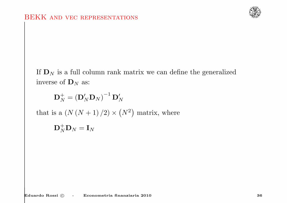
BEKK and vec representations
If DN is a full column rank matrix we can define the generalized
inverse of DN as:
D+N = (D′
NDN )−1
D′
N
that is a (N (N + 1) /2)×(N2)matrix, where
D+NDN = IN
Eduardo Rossi c© - Econometria finanziaria 2010 36

BEKK and vec representations
This implies that premultiplying by D+N
vech (Ht) = vech(CC′) +D+N
(q∑
i=1
(Ai ⊗Ai)
)DNvech(ǫt−iǫ
′
t−i)
+D+N
(p∑
i=1
(Bi ⊗Bi)
)DNvech(Ht−i)
• The vech model implied by any given BEKK model is unique,
while the converse is not true.
• The transformation from a vech model to a BEKK model (when
it exists) is not unique, because for a given A∗
1 the choice of A1
is not unique.
Eduardo Rossi c© - Econometria finanziaria 2010 37

BEKK and vec representations
• This can be seen recognizing that (Ai ⊗Ai) = (−Ai ⊗−Ai) so
while A∗
i = D+N (Ai ⊗Ai)DN is unique, the choice of Ai is not
unique. It can also be shown that all positive definite diagonal
vech models can be written in the BEKK framework.
Given Ai diagonal matrix, then D+N (Ai ⊗Ai)DN is also diagonal,
with diagonal elements given by aiiajj (1 ≤ j ≤ i ≤ N) (See Magnus).
Eduardo Rossi c© - Econometria finanziaria 2010 38

MGARCH-Covariance Stationarity
Given the vech model
vech (Ht) = W +A∗ (L) vech (εtε′
t) +B∗ (L) vech (Ht)
the necessary and sufficient condition for covariance stationary of
{εt} is that all the eigenvalues of A∗ (1) +B∗ (1) are less than one in
modulus. But defining
A∗ (1) = D+N
(q∑
i=1
(Ai ⊗Ai)
)DN
B∗ (1) = D+N
(q∑
i=1
(Bi ⊗Bi)
)DN
Eduardo Rossi c© - Econometria finanziaria 2010 39

MGARCH-Covariance Stationarity
This implies also that in the BEKK model, {ǫt} is covariance
stationary if and only if all the eigenvalues of
D+N
(q∑
i=1
(Ai ⊗Ai)
)DN +D+
N
(p∑
i=1
(Bi ⊗Bi)
)DN
are less than one in modulus.
Let λ1, . . . , λN be the eigenvalues of Ai, the eigenvalues of
D+N
(q∑
i=1
(Ai ⊗Ai)
)DN
are λiλj (1 ≤ j ≤ i ≤ N) (Magnus).
Eduardo Rossi c© - Econometria finanziaria 2010 40

MGARCH(1,1)-BEKK Unconditional Covariance Matrix
BEKK model
vec (ǫtǫ′
t) = vec (CC′) + (A1 ⊗A1) vec(ǫt−1ǫ
′
t−1
)
+(B1 ⊗B1)[vec(ǫt−1ǫ
′
t−1
)− vec (Vt−1)
]+ vec (Vt)
E [vec (ǫtǫ′
t)] = vec (CC′)+[(A1 ⊗A1) + (B1 ⊗B1)]E[vec(ǫt−1ǫ
′
t−1
)]
vec (Σ) = [IN2 − (A1 ⊗A1)− (B1 ⊗B1)]−1 vec (CC′)
or in vech representation as
DNvech (E (ǫtǫ′
t)) = DNvech (CC′) + (A1 ⊗A1)DNvech(E(ǫt−1ǫ
′
t−1
))
+(B1 ⊗B1)DNvech(E(ǫt−1ǫ
′
t−1
))
vech (Σ) =[IN∗ −D+
N (A1 ⊗A1)DN −D+N (B1 ⊗B1)DN
]−1
vech (CC′)
N∗ = N (N + 1) /2.
Eduardo Rossi c© - Econometria finanziaria 2010 41

MGARCH(1,1)-Diagonal models - Covariance stationarity
• The diagonal vech model is stationary if and only if the sum
a∗ii + b∗ii < 1 for all i.
• In the diagonal BEKK model the covariance stationary condition
is that a2ii + b2ii < 1.
Only in the case of diagonal models the stationarity properties are
determined solely by the diagonal elements of the Ai and Bi
matrices.
Eduardo Rossi c© - Econometria finanziaria 2010 42

Asymmetric MGARCH-in-mean model
A general multivariate model can be written as:
yt = µ+Π (L)yt−1 +Ψxt−1 +Λvech (Ht) + ǫt (4)
yt : (N × 1)
Π (L) = Π1 +Π2L+ · · ·+ΠkLk−1 (N ×N)
Ψ : (N × L)
Λ : (N ×N (N + 1) /2)
xt : (L× 1)
Eduardo Rossi c© - Econometria finanziaria 2010 43

Asymmetric MGARCH-in-mean model
xt−1 contains predetermined variables. ǫt is the vector of innovation
with respect to the information set formed exclusively of past
realizations of yt.
Ht = Et−1 (ǫtǫ′
t)
Ht = CC′ +
q∑
i=1
Ai (ǫt−i + γ) (ǫt−i + γ)′
A′
i +
p∑
j=1
BjHt−jB′
j (5)
Eduardo Rossi c© - Econometria finanziaria 2010 44

Asymmetric MGARCH-in-mean model
We can consider a multivariate generalization of the size effect and
sign effect:
Ht = CC′+A1ǫt−1ǫ′
t−1A′
1+B1Ht−1B′
1+Dvt−1v′
t−1D′+Gǫt−1ǫ
′
t−1G′
where vt = |zt| − E |zt|, with zit = εit/√hii,t and
G =
I (ε1t−1 < 0) g11 0 . . . 0
0. . .
......
. . . 0
0 . . . 0 I (εNt−1 < 0) gNN
Eduardo Rossi c© - Econometria finanziaria 2010 45

Asymmetric MGARCH-in-mean model
When N = 2
vt−1v′
t−1 =
∣
∣
∣ε1t−1/
√
h11,t−1
∣
∣
∣− E
∣
∣
∣ε1t−1/
√
h11,t−1
∣
∣
∣
∣
∣
∣ε2t−1/
√
h22,t−1
∣
∣
∣− E
∣
∣
∣ε2t−1/
√
h22,t−1
∣
∣
∣
×
∣
∣
∣ε1t−1/
√
h11,t−1
∣
∣
∣− E
∣
∣
∣ε1t−1/
√
h11,t−1
∣
∣
∣
∣
∣
∣ε2t−1/
√
h22,t−1
∣
∣
∣− E
∣
∣
∣ε2t−1/
√
h22,t−1
∣
∣
∣
′
=
(|z1t| − E |z1t|)2 (|z1t| − E |z1t|) (|z2t| − E |z2t|)
(|z2t| − E |z2t|) (|z1t| − E |z1t|) (|z2t| − E |z2t|)2
Eduardo Rossi c© - Econometria finanziaria 2010 46

Asymmetric MGARCH-in-mean model
Gǫt−1ǫ′
t−1G′ =
g∗211ε
21t−1 g∗11g
∗
22ε1t−1ε2t−1
g∗11g∗
22ε1t−1ε2t−1 g∗222ε22t−1
=
I (ε1t−1 < 0) g211ε
21t−1 δ12g11g22ε1t−1ε2t−1
δ12g11g22ε1t−1ε2t−1 I (ε2t−1 < 0) g222ε22t−1
δ12 = I (ε1t−1 < 0) I (ε2t−1 < 0)
Eduardo Rossi c© - Econometria finanziaria 2010 47
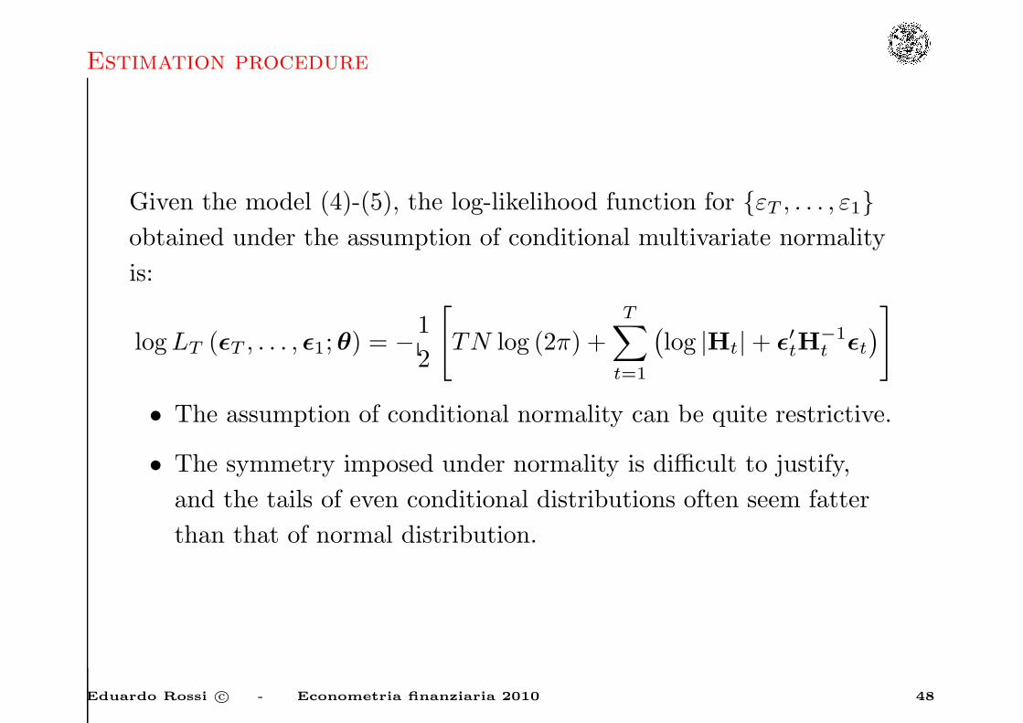
Estimation procedure
Given the model (4)-(5), the log-likelihood function for {εT , . . . , ε1}obtained under the assumption of conditional multivariate normality
is:
logLT (ǫT , . . . , ǫ1; θ) = −1
2
[TN log (2π) +
T∑
t=1
(log |Ht|+ ǫ′tH
−1t ǫt
)]
• The assumption of conditional normality can be quite restrictive.
• The symmetry imposed under normality is difficult to justify,
and the tails of even conditional distributions often seem fatter
than that of normal distribution.
Eduardo Rossi c© - Econometria finanziaria 2010 48

Estimation procedure
Let {(yt,xt) : t = 1, 2, . . .} be a sequence of observable random
vectors with yt (N × 1) and xt (L× 1).
The vector yt contains the ”endogenous” variables and xt contains
contemporaneous ”exogenous” variables.
wt = (xt,yt−1,xt−1, . . . , y1,x1) .
The conditional mean and variance functions are jointly
parameterized by a finite dimensional vector θ:
{µt (wt, θ) , θ ∈ Θ}
{Ht (wt, θ) , θ ∈ Θ}where Θ ⊂ R
P and µt and Ht are known functions of wt and θ.
Eduardo Rossi c© - Econometria finanziaria 2010 49

Estimation procedure
The validity of most of the inference procedures is proven under the
null hypothesis that the first two conditional moments are correctly
specified, for some θ0 ∈ Θ,
E (yt |wt ) = µt (wt, θ0)
V ar (yt |wt ) = Ht (wt, θ0) t = 1, 2, . . .
The procedure most often used to estimate θ0 is the maximization of
a likelihood function that is constructed under the assumption that
yt |wt ∼ N (µt,Ht).
The approach taken here is the same, but the subsequent analysis
does not assume that yt has a conditional normal distribution.
Eduardo Rossi c© - Econometria finanziaria 2010 50

Estimation procedure
For observation t the quasi-conditional log-likelihood is
lt (θ;yt, wt) = −N2ln (2π)− 1
2ln |Ht (wt, θ)|
−1
2(yt − µt (wt, θ))
′
H−1t (wt, θ) (yt − µt (wt, θ))
Letting
ǫt (yt, wt, θ0) ≡ yt − µt (wt, θ) : (N × 1)
denote the residual function
lt (θ) = −N2log (2π)− 1
2log |Ht (θ)| −
1
2ǫ′t (θ)H
−1t (θ) ǫt (θ)
logLT (θ) =
T∑
t=1
lt (θ)
Eduardo Rossi c© - Econometria finanziaria 2010 51

Estimation procedure
If µt (wt, θ) and Ht (wt, θ) are differentiable on Θ for all relevant wt,
and if Ht (wt, θ) is nonsingular with probability one for all θ ∈ Θ,
then the differentiation of the loglik yields the (1× P ) score function
st (θ):
st (θ)′
= ∇θlt (θ)′ −∇θµt (θ)
′
H−1t (θ) ǫt (θ) +
1
2∇θHt (θ)
′[H−1
t (θ)⊗H−1t (θ)
]vec
[ǫt (θ) ǫt (θ)
′ −Ht (θ)]
where
∇θµt (θ) : (N × P )
∇θHt (θ) :(N2 × P
)
Eduardo Rossi c© - Econometria finanziaria 2010 52

Estimation procedure
If the first conditional two moments are correctly specified, the true
error vector is defined as
ǫ0t ≡ ǫt (θ0) = yt − µt (wt, θ0)
and E(ǫ0t |wt
)= 0,
E(ǫ0t ǫ
0′t |wt
)= Ht (wt, θ0)
It follows that under correct specification of the first two conditional
moments of yt given wt:
E [st (θ0) |wt ] = 0
The score evaluated at the true parameter is a vector of martingale
difference with respect to the σ − fields {σ (yt, wt) : t = 1, 2, . . .}.This result can be used to establish weak consistency of the
quasi-maximum likelihood estimator (QMLE).
Eduardo Rossi c© - Econometria finanziaria 2010 53

Estimation procedure
For robust inference we also need an expression for the hessian
ht (θ) of lt (θ). Define the positive semidefinite matrix
at (θ0) = −E [∇θst (θ0) |wt ] = E [−ht (θ0) |wt ] : (P × P )
at (θ0) = ∇θµt (θ0)′
H−1t (θ0)∇θµt (θ0)
+1
2∇θHt (θ)
′[H−1
t (θ)⊗H−1t (θ)
]∇θHt (θ)
When the normality assumption holds the matrix at (θ0) is the
conditional information matrix. However, if yt does not have a
conditional normal distribution then
V ar [st (θ0) |wt ] 6= at (θ0)
and the information matrix equality is violated.
Eduardo Rossi c© - Econometria finanziaria 2010 54

Estimation procedure
The QMLE has the following properties:
[A0−1
T B0TA
0−1T
]−1/2√T(θT − θ0
)d→ N (0, IP )
where
A0T ≡ − 1
T
T∑
t=1
E [ht (θ0)] =1
T
T∑
t=1
E [at (θ0)]
and
B0T ≡ V ar
[T−1/2ST (θ0)
]=
1
T
T∑
t=1
E[st (θ0)
′ st (θ0)]
in addition
AT −A0T
p→ 0
BT −B0T
p→ 0
Eduardo Rossi c© - Econometria finanziaria 2010 55

Estimation procedure
The matrix A−1T BT A
−1T is a consistent estimator od the robust
asymptotic covariance matrix of√T(θT − θ0
).
In practice,
θT ≈ N(θ, A−1
T BT A−1T /T
)
Under normality, the variance estimator can be replaced by A−1T /T
(Hessian form) or B−1T /T (outer product of the gradient form).
Eduardo Rossi c© - Econometria finanziaria 2010 56
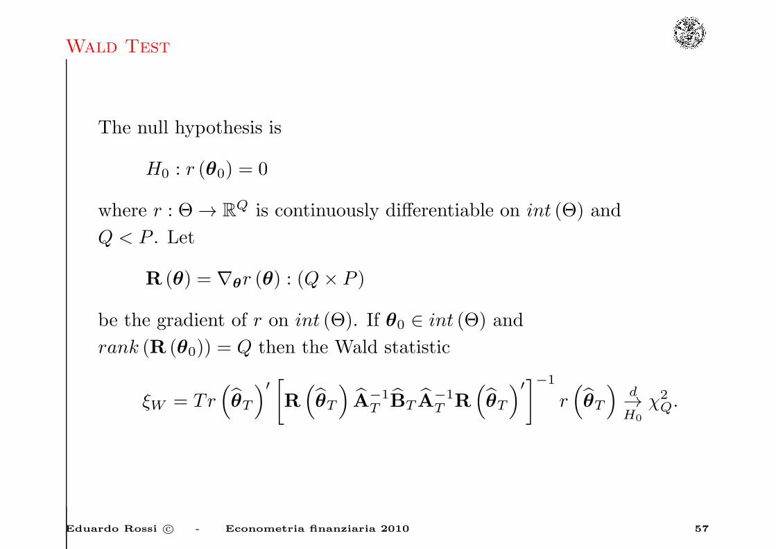
Wald Test
The null hypothesis is
H0 : r (θ0) = 0
where r : Θ → RQ is continuously differentiable on int (Θ) and
Q < P . Let
R (θ) = ∇θr (θ) : (Q× P )
be the gradient of r on int (Θ). If θ0 ∈ int (Θ) and
rank (R (θ0)) = Q then the Wald statistic
ξW = Tr(θT
)′
[R(θT
)A−1
T BT A−1T R
(θT
)′
]−1
r(θT
)d→H0
χ2Q.
Eduardo Rossi c© - Econometria finanziaria 2010 57

Factor-GARCH
The Factor GARCH model, introduced by Engle et al. (1990), can be
thought of as an alternative simple parametrization of the BEKK
model. Suppose that the (N × 1) yt has a factor structure with K
factors given by the K × 1 vector ft and a time invariant factor
loadings given by the N ×K matrix B:
yt = Bft + ǫt
Eduardo Rossi c© - Econometria finanziaria 2010 58

Factor-GARCH
Assume that the idiosyncratic shocks ǫt have conditional covariance
matrix Ψ which is constant in time and positive semidefinite, and
that the common factors are characterized by
Et−1 (ft) = 0
Et−1 (ftf′
t) = Λt
Λt = diag (λ1, . . . , λK) and positive definite. The conditioning set is
{yt−1, ft−1, . . . ,y1, f1}. Also suppose that E (ftǫ′
t) = 0. The
conditional covariance matrix of yt equals
Et−1 (yty′
t) = Ht = Ψ+BΛtB′ = Ψ+
K∑
k=1
βkβ′
kλkt
where βk denotes the kth column in B. Thus, there are K statistics
which determine the full covariance matrix.
Eduardo Rossi c© - Econometria finanziaria 2010 59
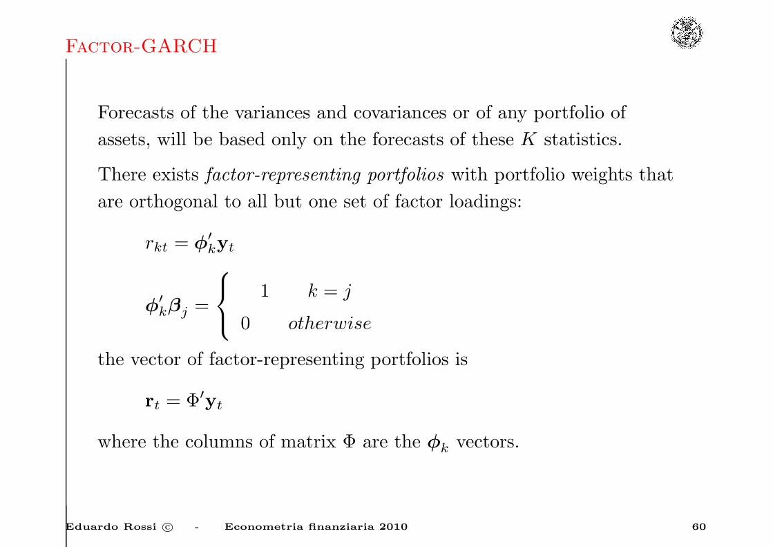
Factor-GARCH
Forecasts of the variances and covariances or of any portfolio of
assets, will be based only on the forecasts of these K statistics.
There exists factor-representing portfolios with portfolio weights that
are orthogonal to all but one set of factor loadings:
rkt = φ′
kyt
φ′
kβj =
1 k = j
0 otherwise
the vector of factor-representing portfolios is
rt = Φ′yt
where the columns of matrix Φ are the φk vectors.
Eduardo Rossi c© - Econometria finanziaria 2010 60

Factor-GARCH
The conditional variance of rkt is given by
Vart−1 (rkt) = φ′
kEt−1 (yty′
t)φk = φ′
kHtφk
= φ′
k (Ψ +BΛtB′)φk
= ψk + λkt
where ψk = φ′
kΨφk. The portfolio has the exact time variation as the
factors, which is why they are called factor-representing portfolios. In
order to estimate this model, the dependence of the λkt’s upon the
past information set must also be parameterized:
θkt ≡ φ′
kHtφk = V art−1 (rkt) = ψk + λkt
So we get that
K∑
k=1
βkβ′
kθkt =K∑
k=1
βkβ′
kψk +K∑
k=1
βkβ′
kλkt
Eduardo Rossi c© - Econometria finanziaria 2010 61
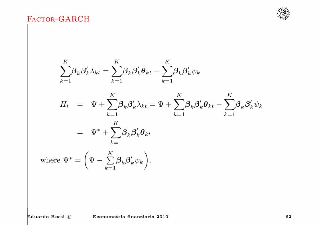
Factor-GARCH
K∑
k=1
βkβ′
kλkt =K∑
k=1
βkβ′
kθkt −K∑
k=1
βkβ′
kψk
Ht = Ψ+K∑
k=1
βkβ′
kλkt = Ψ+K∑
k=1
βkβ′
kθkt −K∑
k=1
βkβ′
kψk
= Ψ∗ +
K∑
k=1
βkβ′
kθkt
where Ψ∗ =
(Ψ−
K∑k=1
βkβ′
kψk
).
Eduardo Rossi c© - Econometria finanziaria 2010 62

Factor-GARCH
The simplest assumption is that there is a set of factor-representing
portfolios with univariate GARCH(1,1) representations. The
conditional variance θkt follows a GARCH(1,1) process
θkt = ωk + αk
(φ′
kǫt−1
)2+ γkEt−2
(r2kt−1
)
θkt = ωk + αkφ′
k
(ǫt−1ǫ
′
t−1
)φk + γkEt−2
[(φ′
kyt) (
φ′
kyt)]
θkt = ωk + αkφ′
k
(ǫt−1ǫ
′
t−1
)φk + γk
[φ′
kEt−2 (yty′
t)φk
]
θkt = ωk + αkφ′
k
(ǫt−1ǫ
′
t−1
)φk + γk
[φ′
kHt−1φk
]
Eduardo Rossi c© - Econometria finanziaria 2010 63

Factor-GARCH
The conditional variance-covariance matrix of yt can be written as
Ht = Ψ∗ +K∑
k=1
βkβ′
kθkt
= Ψ∗ +K∑
k=1
βkβ′
k
{ωk + αk
[φ′
k
(ǫt−1ǫ
′
t−1
)φk
]+ γk
[φ′
kHt−1φk
]}
=
(Ψ∗ +
K∑
k=1
βkβ′
kωk
)+
K∑
k=1
βkβ′
k
{αk
[φ′
k
(ǫt−1ǫ
′
t−1
)φk
]+ γk
[φ′
kHt−1φk
Ht = Γ +K∑
k=1
βkβ′
kθkt
Eduardo Rossi c© - Econometria finanziaria 2010 64
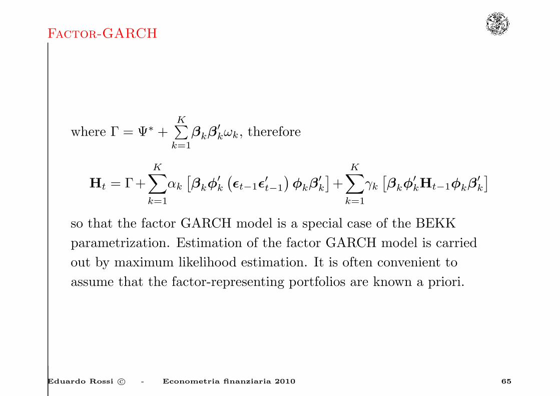
Factor-GARCH
where Γ = Ψ∗ +K∑
k=1
βkβ′
kωk, therefore
Ht = Γ+K∑
k=1
αk
[βkφ
′
k
(ǫt−1ǫ
′
t−1
)φkβ
′
k
]+
K∑
k=1
γk[βkφ
′
kHt−1φkβ′
k
]
so that the factor GARCH model is a special case of the BEKK
parametrization. Estimation of the factor GARCH model is carried
out by maximum likelihood estimation. It is often convenient to
assume that the factor-representing portfolios are known a priori.
Eduardo Rossi c© - Econometria finanziaria 2010 65

Orthogonal-GARCH model
The orthogonal models are particular factor models. They are based
on the assumption that the observed data can be obtained by a linear
transformation of a set of uncorrelated components.
The components are the principal components of the data, or a
subset of them.
The diagonal matrix V contains the empirical variances of yt:
V = diag{s21, . . . , s2N}
the standardized returns are
ut = V−1/2yt
E[ut] = 0 E[utu′
t] = R
Eduardo Rossi c© - Econometria finanziaria 2010 66

Orthogonal-GARCH model
The sample correlation matrix can be decomposed as:
R = PΛP′
P is the orthonormal eigenvectors matrix, Λ is the diagonal matrix of
the eigenvalues:
Λ = diag{λ1, . . . , λN}
ranked in descending order.
Eduardo Rossi c© - Econometria finanziaria 2010 67

Orthogonal-GARCH model
P satisfies:
P′ = P−1 P′P = IN PP′ = IN
It follows that
R = PΛ1/2Λ1/2P′ = LL′
L = PΛ1/2
Principal components
ft = L−1ut
E[ftf′
t ] = L−1E[utu′
t]L−1′ = L−1RL−1′
= L−1LL′L′−1 = IN
Eduardo Rossi c© - Econometria finanziaria 2010 68

Orthogonal-GARCH model
Assuming
Et−1[ftf′
t ] = Qt = diag(σ2f1,t , . . . , σ
2fN,t
)
Qt is a diagonal matrix.
σ2fi,t ∼ GARCH(p,q) i = 1, 2, . . . , N
Et−1[utu′
t] = Et−1[Lftf′
tL′] = LQtL
′
Et−1[yty′
t] = Et−1[V1/2utu
′
tV1/2] = V1/2LQtL
′V1/2
Eduardo Rossi c© - Econometria finanziaria 2010 69

Orthogonal-GARCH model
We can work with a reduced number m < N of principal components
(eigenvalues), those which explain most of the variation in the data.
L−1 is replaced by a matrix (m×N):
Λ−1/2m P′
m
Pm is a matrix (N ×m) containing the m eigenvectors of P
corresponding to the m largest eigenvalues.
fmt = Λ−1/2m P′
mut
where fmt = [f1t, . . . , fmt]
Et−1[fmt ] = 0
Et−1[fmt fm
′
t ] = Qt = diag(σ2f1,t , . . . , σ
2fm,t
)
Eduardo Rossi c© - Econometria finanziaria 2010 70
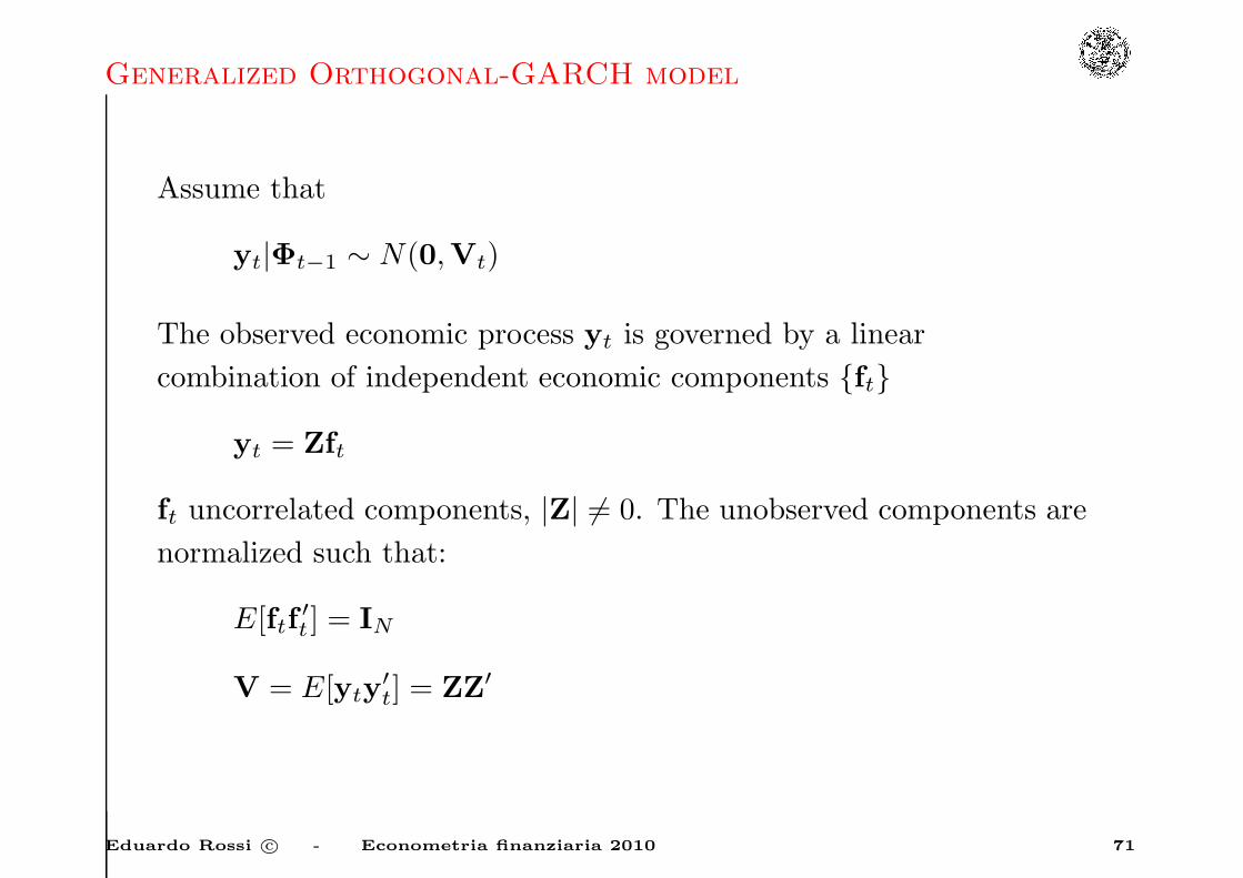
Generalized Orthogonal-GARCH model
Assume that
yt|Φt−1 ∼ N(0,Vt)
The observed economic process yt is governed by a linear
combination of independent economic components {ft}
yt = Zft
ft uncorrelated components, |Z| 6= 0. The unobserved components are
normalized such that:
E[ftf′
t ] = IN
V = E[yty′
t] = ZZ′
Eduardo Rossi c© - Econometria finanziaria 2010 71

Generalized Orthogonal-GARCH model
Vt = Et−1[yty′
t] = ZEt−1[ftf′
t]Z′ = ZHtZ
′
Ht = diag{h1,t, . . . , hN,t}
hi,t = (1− α1 − βi) + αiy2i,t−i + βihi,t−1 i = 1, . . . , N
V = E[Vt] = ZHZ′
H diagonal. The diagonal decomposition of the unconditional
covariance matrix:
V = PΛP′
P: orthogonal matrix, O-GARCH estimator for Z, is only guaranteed
to coincide with Z, when the diagonal elements of H are all distinct.
Eduardo Rossi c© - Econometria finanziaria 2010 72

Generalized Orthogonal-GARCH model
Suppose that H = I
V = E[Vt] = ZIZ′ = ZZ′
The matrix Z is no longer identified by the eigenvector matrix of V
as for every orthogonal matrix Q we have
(ZQ)(ZQ)′ = I
The matrix Z is well identified when conditional information is taken
into account. Based on singular value decomposition:
PΛ1/2U0 = Z
Let the estimator of U0 be U. We restrict
|U| = 1.
Eduardo Rossi c© - Econometria finanziaria 2010 73
Generalized Orthogonal-GARCH model
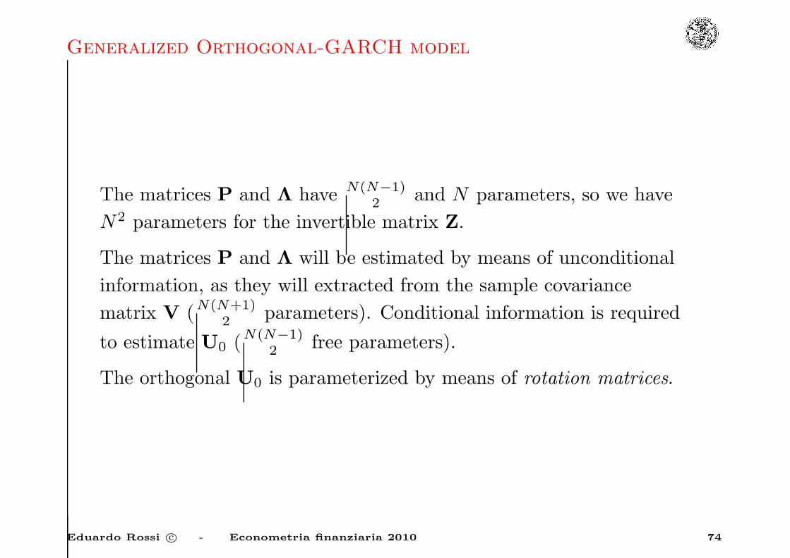
The matrices P and Λ have N(N−1)2 and N parameters, so we have
N2 parameters for the invertible matrix Z.
The matrices P and Λ will be estimated by means of unconditional
information, as they will extracted from the sample covariance
matrix V (N(N+1)2 parameters). Conditional information is required
to estimate U0 (N(N−1)2 free parameters).
The orthogonal U0 is parameterized by means of rotation matrices.
Eduardo Rossi c© - Econometria finanziaria 2010 74

Generalized Orthogonal-GARCH model
Rotation matrix: Grs, (N ×N), r, s ∈ N, r < s ≤ N :
Grs = {gij}grr = gss = cos(θ)
gii = 1 i = 1, . . . , N i 6= r, s
gsr = − sin(θ)
grs = sin(θ)
and all other elements are zero. N = 3:
G12 =
cos(θ) sin(θ) 0
− sin(θ) cos(θ) 0
0 0 1
Eduardo Rossi c© - Econometria finanziaria 2010 75

Generalized Orthogonal-GARCH model
Every N-dimensional orthogonal matrix U with det(U) = 1 can be
represented as a product of N(N−1)2 rotation matrices:
U =∏
i<j
Gij(θij) − π ≤ θij ≤ π
Gij(θij) performs a rotation in the plane spanned by the i-th and the
j-th vectors of the canonical basis of RN over an angle δij .
N = 3:
U = G12G13G23
Eduardo Rossi c© - Econometria finanziaria 2010 76

Generalized Orthogonal-GARCH model
Time-varying conditional correlations:
Rt = D−1t VtD
−1t
Dt = (Vt ⊙ Im)1/2
N = 2
Z =
1 0
cos θ sin θ
θ measures the extent to which the uncorrelated components are
mapped in the same direction. For θ = 0 the mapping in not
invertible, yielding perfect correlation between the observed variables,
whereas θ = π2 , Z = I so that observed variables are completely
uncorrelated.
Eduardo Rossi c© - Econometria finanziaria 2010 77

Generalized Orthogonal-GARCH model
ρt =Covt−1(y1t, y2t)√
V art−1(y1t)√V art−1(y2t)
In this example the conditional correlation is:
ρt =h1t cos (θ)
√h1t
√h1t cos2 (θ) + h2t sin
2 (θ)
=cos (θ)√
cos2 (θ) + h1t
h2tsin2 (θ)
=1√
1 + zt tan2 (θ)
where zt =h1t
h2t.
Note that a constant linkage Zθ gives rise to time-varying correlations
between the observed variables. These correlations rise on average
when the components are mapped more in the same direction.
Eduardo Rossi c© - Econometria finanziaria 2010 78
Generalized Orthogonal-GARCH model
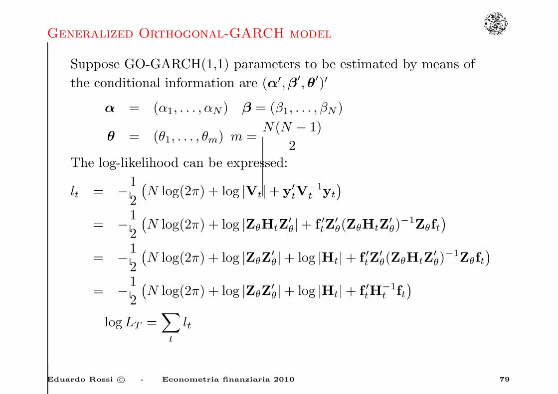
Suppose GO-GARCH(1,1) parameters to be estimated by means of
the conditional information are (α′,β′, θ′)′
α = (α1, . . . , αN ) β = (β1, . . . , βN )
θ = (θ1, . . . , θm) m =N(N − 1)
2The log-likelihood can be expressed:
lt = −1
2
(N log(2π) + log |Vt|+ y′
tV−1t yt
)
= −1
2
(N log(2π) + log |ZθHtZ
′
θ|+ f ′tZ′
θ(ZθHtZ′
θ)−1Zθft
)
= −1
2
(N log(2π) + log |ZθZ
′
θ|+ log |Ht|+ f ′tZ′
θ(ZθHtZ′
θ)−1Zθft
)
= −1
2
(N log(2π) + log |ZθZ
′
θ|+ log |Ht|+ f ′tH−1t ft
)
logLT =∑
t
lt
Eduardo Rossi c© - Econometria finanziaria 2010 79

Generalized Orthogonal-GARCH model
Two-step estimation
1. Zθ = PΛ1/2U0 where P and Λ from the sample covariance
matrix:
V = PΛP′
Zθ = PΛ1/2U
where
U =∏
i<j
Gij(θij) − π ≤ θij ≤ π
2. Estimate (α′,β′, θ′)′ by maximizing the logLT .
Eduardo Rossi c© - Econometria finanziaria 2010 80

MGARCH -The Constant Conditional Correlations Model
• These models are based on a decomposition of the Ht.
• The conditional var-cov matrix is expressed as
Ht = DtRtDt
where Rt is possibly time-varying.
• Conditional correlations and variances are separately modeled.
Eduardo Rossi c© - Econometria finanziaria 2010 81

MGARCH -The Constant Conditional Correlations Model
Bollerslev (1990) Constant Conditional Correlations model:
The time-varying conditional covariances are parameterized to be
proportional to the product of the corresponding conditional
standard deviations. The model assumptions are:
Et−1 [ǫtǫ′
t] = Ht
{Ht}ii = hit i = 1, . . . , N
{Ht}ij = hijt = ρijh1/2it h
1/2jt i 6= j i, j = 1, . . . , N
Dt = diag {h1t, . . . , hNt}
Eduardo Rossi c© - Econometria finanziaria 2010 82
MGARCH -The Constant Conditional Correlations Model
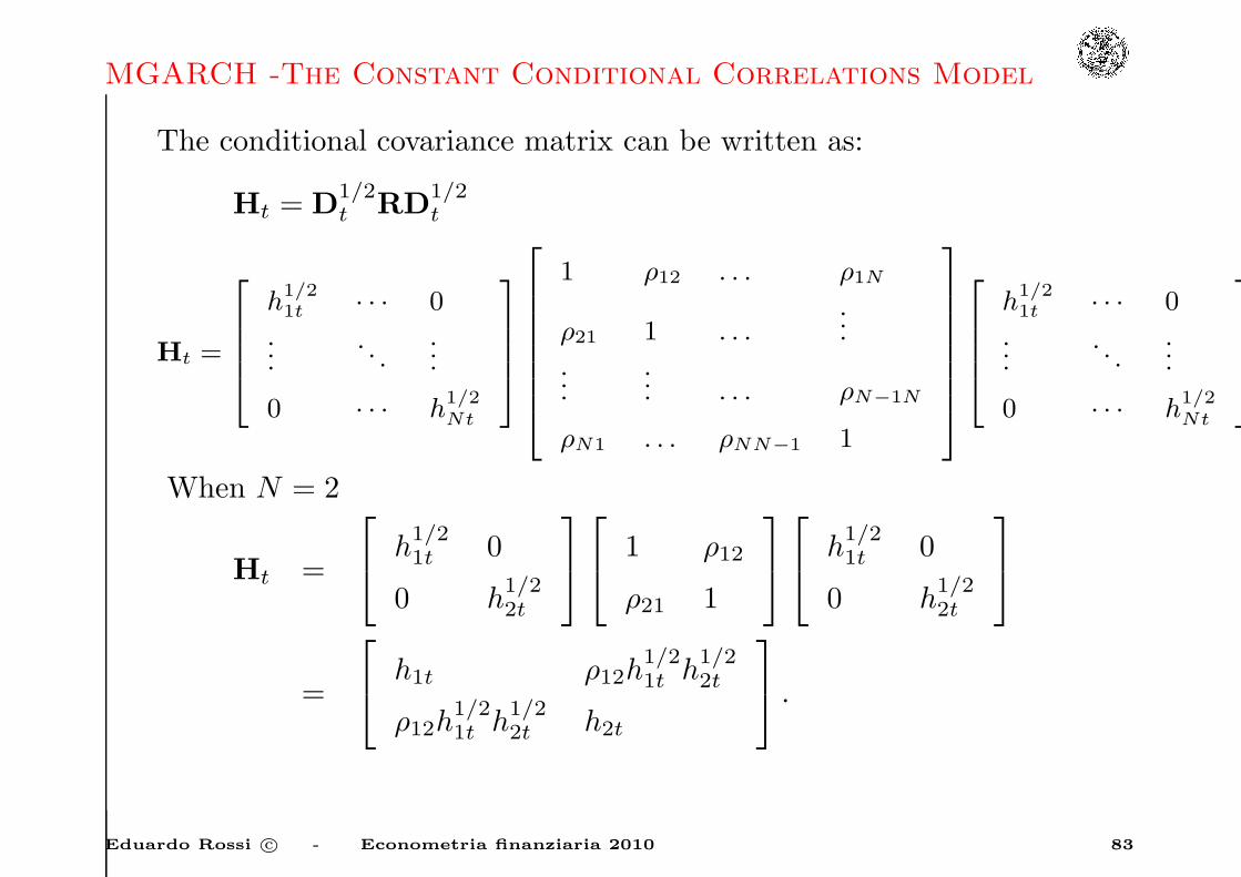
The conditional covariance matrix can be written as:
Ht = D1/2t RD
1/2t
Ht =
h1/21t · · · 0
.... . .
...
0 · · · h1/2Nt
1 ρ12 . . . ρ1N
ρ21 1 . . ....
...... . . . ρN−1N
ρN1 . . . ρNN−1 1
h1/21t · · · 0
.... . .
...
0 · · · h1/2Nt
When N = 2
Ht =
h
1/21t 0
0 h1/22t
1 ρ12
ρ21 1
h
1/21t 0
0 h1/22t
=
h1t ρ12h
1/21t h
1/22t
ρ12h1/21t h
1/22t h2t
.
Eduardo Rossi c© - Econometria finanziaria 2010 83

MGARCH -The Constant Conditional Correlations Model
• The sequence of conditional covariance matrices {Ht} is
guaranteed to be positive definite a.s. for all t, If the conditional
variances along the diagonal in the Dt matrices are all positive,
and the conditional correlation matrix R is positive definite
• Furthermore the inverse of Ht is given by
H−1t = D
−1/2t R−1D
−1/2t .
When calculating the log-likelihood function only one matrix
inversion is required for each evaluation.
• CCC is generally estimated in two steps:
1. conditional variances are estimated employing the marginal
likelihoods
2. R is estimated using the sample estimator of standardized
residuals D−1t yt (assuming µt = 0).
Eduardo Rossi c© - Econometria finanziaria 2010 84

MGARCH -The Constant Conditional Correlations Model
• The CCC solves the curse of dimensionality problem of
MGARCH models
• The number of parameters is O(N2) but these are not jointly
estimated. The two-step estimation procedure impacts on the
computational issues.
• Asymptotic properties of QMLE estimators verified in McAleer
and Ling (2003).
Eduardo Rossi c© - Econometria finanziaria 2010 85

The Dynamic Conditional Correlation GARCH Model
The CCC has two main limitations:
1. No spillover neither feedback effects across conditional variances
2. Correlations are static
The evolution of CCC is the Dynamic Conditional Correlation
(DCC) Model of Engle (2002). The DCC is an extension of the
Bollerslev’s CCC Model.
Eduardo Rossi c© - Econometria finanziaria 2010 86
The Dynamic Conditional Correlation GARCH Model
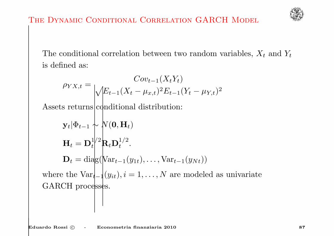
The conditional correlation between two random variables, Xt and Yt
is defined as:
ρY X,t =Covt−1(XtYt)√
Et−1(Xt − µx,t)2Et−1(Yt − µY,t)2
Assets returns conditional distribution:
yt|Φt−1 ∼ N(0,Ht)
Ht = D1/2t RtD
1/2t .
Dt = diag(Vart−1(y1t), . . . ,Vart−1(yNt))
where the Vart−1(yit), i = 1, . . . , N are modeled as univariate
GARCH processes.
Eduardo Rossi c© - Econometria finanziaria 2010 87

The Dynamic Conditional Correlation GARCH Model
The standardized returns are:
ηt = D−1/2t yt
Et−1(ηtη′
t) = D−1/2t HtD
−1/2t = Rt = {ρij,t}
we can use the conditional variance of ηt to describe the conditional
correlation of yt.
The conditional correlation estimator is
ρij,t =qij,t√qii,tqjj,t
.
Where qij,t are assumed to follow a GARCH(1,1) model
qij,t = ρij + α(ηi,t−1ηj,t−1 − ρij) + β(qij,t−1 − ρij) (6)
The term ρij is not the unconditional correlation between ηit and ηjt;
the unconditional correlation between ηit and ηjt has no closed form.
Eduardo Rossi c© - Econometria finanziaria 2010 88

The Dynamic Conditional Correlation GARCH Model
Engle (2002) assumes that ρij ≃ qij . However, Aielli (2006) and
Engle et al. (2008) suggest to modify the standard DCC in order to
correct the asymptotic bias which is due to the fact that 1T
∑t ǫtǫ
′
t
does not converge to Q. It is known though that the impact of this is
very small (see Engle and Sheppard (2001)).
Eduardo Rossi c© - Econometria finanziaria 2010 89

The Dynamic Conditional Correlation GARCH Model
The conditional covariance matrix is positive definite, Qt, as long as
it is a weighted average of definite matrices and semidefinite matrices.
To ensure p.-d-ness of Qt we must impose α+ β < 1 In matrix from:
Qt = Q(1− α− β) + α(ηt−1η′
t−1) + β(Qt−1) (7)
where Q is the unconditional covariance matrix of ηt.
Eduardo Rossi c© - Econometria finanziaria 2010 90

The DCC - Correlation targeting
DCC model has correlation targeting, when α+ β < 1
E[Qt] = R
E[Qt] = E[Qt−1]
E[ηtη′
t] = E[Qt]
E[Qt] = Q(1− α− β) + αE[ηt−1η′
t−1] + βE[Qt−1]
E[Qt] = R(1− α− β) + αE[Qt] + βE[Qt]
Eduardo Rossi c© - Econometria finanziaria 2010 91

The DCC - Correlation targeting
Clearly more complex positive definite multivariate GARCH models
could be used for the correlation parameterization as long as the
unconditional moments are set to the sample correlation matrix.
For example, the MARCH family of Ding and Engle (2001) can be
expressed in first order form as:
Qt = Q⊙ (ιι′ −A−B) +A⊙ ǫt−1ǫ′
t−1 +B⊙Qt−1 (8)
where ⊙ denotes the Hadamard product ({A⊙B}ij = aijbij).
Eduardo Rossi c© - Econometria finanziaria 2010 92

The DCC - Correlation targeting
The Generalized-DCC model specification:
Dt = diag{ωi}+ diag{κi} ⊙ yt−1y′
t−1 + diag{λi} ⊙Dt−1
Qt = S⊙ (ιι′ −A−B) +A⊙ ǫt−1ǫ′
t−1 +B⊙Qt−1
Rt = diag{Qt}−1/2Qt diag{Qt}−1/2.
A and B are symmetric matrices.
The assumption of normality gives rise to a likelihood function.
Without this assumption, the estimator will still have the QML
interpretation. The second equation simply expresses the assumption
that each of the assets follows a univariate GARCH process.
Eduardo Rossi c© - Econometria finanziaria 2010 93

The DCC - Correlation targeting
A real square matrix A, is positive definite if and only if
B = A∗−1AA∗−1 is positive definite, with A∗ = diag{A}.In order to ensure that Ht is positive definite we must have that
D−1/2t HtD
−1/2 is positive definite.
Eduardo Rossi c© - Econometria finanziaria 2010 94

The DCC - Correlation targeting
Ht is positive definite ∀t ∈ T , if the following restrictions on the
univariate GARCH parameters are satisfied for all series
i ∈ [1, . . . , N ] :
1. ωi > 0
2. κi and λi such that Dii,t > 0 with probability 1
3. D2ii,0 > 0
4. The roots of 1− κiZ − λiZ are outside the unit circle.
Eduardo Rossi c© - Econometria finanziaria 2010 95

The DCC - Correlation targeting
and the parameters in the DCC satisfy:
1. α ≥ 0
2. β ≥ 0
3. α+ β ≤ 1
4. The minimum eigenvalue of Q0 > δ > 0 (where Q0 must be
positive definite)
Eduardo Rossi c© - Econometria finanziaria 2010 96

The DCC - Correlation targeting
The log-likelihood function can be written as:
logLT = −1
2
T∑
t=1
(N log(2π) + log |Ht|+ r′tH−1t rt)
= −1
2
T∑
t=1
(N log(2π) + log |D1/2t RtD
1/2t |+ r′tD
−1/2t R−1
t D−1/2t rt)
= −1
2
T∑
t=1
(N log(2π) + log |Dt|+ log |Rt|+ ǫ′tR−1t ǫt)
Eduardo Rossi c© - Econometria finanziaria 2010 97

The DCC - Correlation targeting
Adding and subtracting r′tD−1/2t D
−1/2t rt = ǫ′tǫt
logLT = −1
2
T∑
t=1
(N log(2π) + log |Dt|+ r′tD−1/2t D
−1/2t rt
−ǫ′tǫt + log |Rt|+ ǫ′tR−1t ǫt)
= −1
2
T∑
t=1
(N log(2π) + log |Dt|+ r′tD−1t rt)
−1
2
T∑
t=1
(ǫ′tR−1t ǫt − ǫ′tǫt + log |Rt|)
Eduardo Rossi c© - Econometria finanziaria 2010 98

The DCC - Correlation targeting
Volatility component:
LV (θ) ≡ logLV,T (θ) = −1
2
T∑
t=1
(N log(2π) + log |Dt|+ r′tD−1t rt)
Correlation component:
LC(θ,φ) ≡ logLC,T (θ,φ) = −1
2
T∑
t=1
(ǫ′tR−1t ǫt − ǫ′tǫt + log |Rt|)
θ denotes the parameters in Dt and φ the parameters in Rt.
Eduardo Rossi c© - Econometria finanziaria 2010 99

The DCC - Correlation targeting
L(θ,φ) = LV (θ) + LC(θ,φ)
LV (θ) = −1
2
T∑
t=1
N∑
i=1
(log(2π) + log(hi,t) +
r2i,thi,t
).
The likelihood is apparently the sum of individual GARCH
likelihoods, which will be jointly maximized by separately
maximizing each term.
Eduardo Rossi c© - Econometria finanziaria 2010 100

The DCC - Correlation targeting
Two-step procedure:
1.
θ = argmax{LV (θ)}
2.
maxφ
{LC(θ,φ)}.
Under regularity conditions, consistency of the first step will ensure
consistency of the second step. The maximum of the second step will
a function of the first step parameter estimates. If the first step is
consistent then the second step will be too as long as the function is
continuous in a neighborhood of the true parameters.
Eduardo Rossi c© - Econometria finanziaria 2010 101
The DCC - Correlation targeting
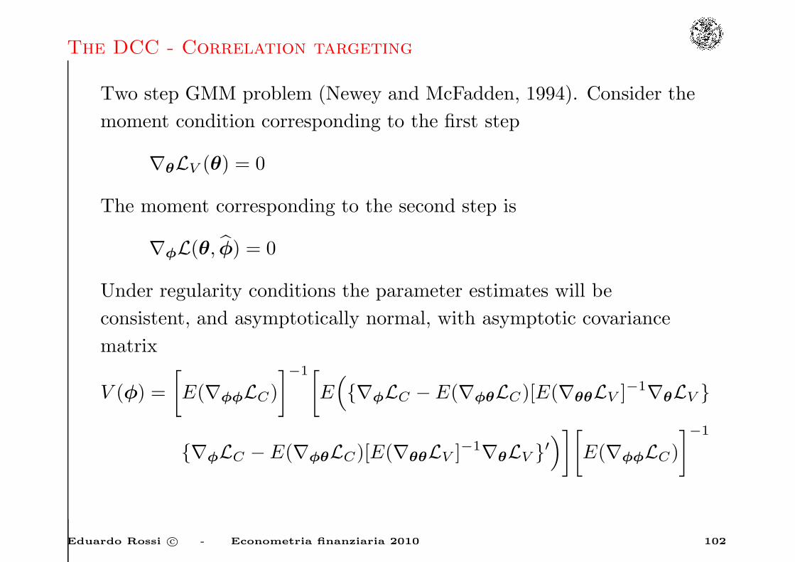
Two step GMM problem (Newey and McFadden, 1994). Consider the
moment condition corresponding to the first step
∇θLV (θ) = 0
The moment corresponding to the second step is
∇φL(θ, φ) = 0
Under regularity conditions the parameter estimates will be
consistent, and asymptotically normal, with asymptotic covariance
matrix
V (φ) =
[E(∇φφLC)
]−1[
E({∇φLC − E(∇φθLC)[E(∇θθLV ]
−1∇θLV }
{∇φLC − E(∇φθLC)[E(∇θθLV ]−1∇θLV }′
)][E(∇φφLC)
]−1
Eduardo Rossi c© - Econometria finanziaria 2010 102