A multivariate heavy-tailed distributionfor ARCH/GARCH residuals

Dimitris N. Politis∗

Department of Mathematics

University of California—San DiegoLa Jolla, CA 92093-0112, USA

email: dpolitis@ucsd.edu

Abstract

A new multivariate heavy-tailed distribution is proposed as an exten-sion of the univariate distribution of Politis (2004). The propertiesof the new distribution are discussed, as well as its effectiveness inmodeling ARCH/GARCH residuals. A practical procedure for multi-parameter numerical maximum likelihood is also given, and a real dataexample is worked out.

JEL codes: C3; C5.

Keywords: Heteroscedasticity, maximum likelihood, time series.

∗Research partially supported by NSF grant SES-04-18136 funded jointly by the Eco-nomics and Statistics Programs of the National Science Foundation.

1

1 INTRODUCTION

Consider univariate data X1, . . . , Xn arising as an observed stretch from afinancial returns time series {Xt, t = 0,±1,±2, . . .} such as the percentagereturns of a stock price, stock index or foreign exchange rate. The returnsseries {Xt} are assumed strictly stationary with mean zero which—from apractical point of view—implies that trends and other nonstationarities havebeen successfully removed. Furthermore, for simplicity the returns series{Xt} will be assumed to have a symmetric1 distribution around zero.

The celebrated ARCH models of Engle (1982) were designed to capturethe phenomenon of volatility clustering in the returns series. An ARCH(p)model can be described by the following equation:

Xt = Zt

√√√√a +p∑

i=1

aiX2t−i (1)

where a, a1, . . . , ap are nonnegative parameters. Since the residuals from afitted ARCH(p) model do not appear to be normally distributed, practition-ers have typically been employing ARCH models with heavy-tailed errors.A popular assumption for the distribution of the Zts is the t-distributionwith degrees of freedom empirically chosen to match the apparent degree ofheavy tails as measured by higher-order moments such as the kurtosis; seee.g. Bollerslev et al. (1992) or Shephard (1996) and the references therein.

Nevertheless, the choice of a t-distribution is quite arbitrary, and thesame is true for other popular heavy-tailed distributions, e.g. the double ex-ponential. For this reason, Politis (2004) developed an implicit ARCH modelthat helps suggest a more natural heavy-tailed distribution for ARCH and/orGARCH residuals; see Bollerslev (1986) for the definition of GARCH models.The motivation for this new distribution is given in Section 2, together witha review of some of its properties. In Section 3, the issue of multivariate datais brought up, and a multivariate version of the new heavy-tailed distributionis proposed. A practical algorithm for multi-parameter numerical maximumlikelihood is given in Section 4 based on an approximate steepest-ascent idea.Section 5 deals in detail with the bivariate paradigm. Finally, a real dataexample is worked out in Section 6.

1Some authors have raised the question of existence of skewness in financial returns;see e.g. Patton (2002) and the references therein. Nevertheless, at least as a first approx-imation, the assumption of symmetry is very useful for model building.

2

2 THE IMPLICIT ARCH MODEL IN THE

UNIVARIATE CASE: A BRIEF REVIEW

Engle’s (1982) original assumption was that the errors Zt in model (1) arei.i.d. N(0, 1). Under that assumption, the residuals

Zt =Xt√

a +∑p

i=1 aiX2t−i

(2)

ought to appear normally distributed; here, a, a1, a2, . . . are estimates of thenonnegative parameters a, a1, a2, . . .. Nevertheless, as previously mentioned,the residuals typically exhibit a degree of heavy tails. In other words, typi-cally there is not a specification for a, a1, a2, . . . that will render the residualsZt normal-looking.

A way to achieve ARCH residuals that appear normal was given in theimplicit ARCH model of Politis (2004) that is defined as:

Xt = Wt

√√√√a + a0X2t +

p∑i=1

aiX2t−i. (3)

When the implicit ARCH model (3) is fitted to the data, the following resid-uals ensue:

Wt =Xt√

a + a0X2t +

∑pi=1 aiX2

t−i

. (4)

As argued in Politis (2004), by contrast to the standard ARCH model (1),there typically always exists here a specification for a, a0, a1, . . . that willrender the residuals Wt normal-looking.2 Hence, it is not unreasonable toassume that the Wt errors in model (3) are i.i.d. N(0, 1).

Technically speaking, however, this is not entirely correct since it is easyto see that the Wts are actually bounded (in absolute value) by 1/

√a0. A

natural way to model the situation where the Wt are thought to be close to

2To see why, note that the specification a = 0, a0 = 1, and ai = 0 for i > 0, correspondsto Wt = sign(Xt) that has kurtosis equal to one. As previously mentioned, specificationswith a0 = 0 typically yield residuals Wt with heavier tails than the normal, i.e., kurtosisbigger than 3. Thus, by the intermediate value theorem, a specification for a, a0, a1, . . .should exist that would render the kurtosis of Wt attaining the intermediate value of 3.

3

N(0, 1) but happen to be bounded is to use a truncated standard normaldistribution, i.e., to assume that the Wt are i.i.d. with probability densitygiven by

φ(x)1{|x| ≤ C0}∫ C0−C0

φ(y)dyfor all x ∈ R (5)

where φ denotes the standard normal density, 1{S} the indicator of set S,and C0 = 1/

√a0. If/when a0 is small enough, the boundedness of Wt is

effectively not noticeable.Note that the only difference between the implicit ARCH model (3) and

the standard ARCH model (1) is the introduction of the term Xt paired witha nonzero coefficient a0 in the right-hand-side of equation (3). It is preciselythis Xt term appearing in both sides of (3) that gives the characterization‘implicit’ to model (3).

Nevertheless, we can solve equation (3) for Xt, to obtain:

Xt = Ut

√√√√a +p∑

i=1

aiX2t−i (6)

where

Ut =Wt√

1 − a0W 2t

. (7)

Thus, the implicit ARCH model (3) is seen to be tantamount to the regularARCH(p) model (6) associated with the new innovation term Ut.

However, if Wt is assumed to follow the truncated standard normal distri-bution (5), then the change of variable (7) implies that the innovation termUt appearing in the ARCH model (6) has the density f(u; a0, 1) defined as:

f(u; a0, 1) =(1 + a0u

2)−3/2 exp(− u2

2(1+a0u2))

√2π

(Φ(1/

√a0) − Φ(−1/

√a0)

) for all u ∈ R (8)

where Φ denotes the standard normal distribution function. Equation (8)gives the univariate heavy-tailed density for ARCH residuals proposed inPolitis (2004).

Note that the density f(u; a0, 1) can be scaled to create a two-parameterfamily of densities with typical member given by

f(x; a0, c) =1

cf(

x

c; a0, 1) for all x ∈ R. (9)

4

The nonnegative parameter a0 is a shape parameter having to do with thedegree of heavy tails, while the positive parameter c represents scale; notethat f(u; a0, 1) → φ(u) as a0 → 0.

It is apparent that f(u; a0, c) has heavy tails. Except for the extreme casewhen a0 = 0 and all moments are finite, in general moments are finite onlyup to (almost) order two. In other words, if a random variable U follows thedensity f(u; a0, c) with a0, c > 0, then it is easy to see that

E|U |d < ∞ for all d ∈ [0, 2) but E|U |d = ∞ for all d ∈ [2,∞).

Thus, working with the heavy-tailed density f(u; a0, c) is associated with theconviction that financial returns have higher-order moments that are infinite;Politis (2003, 2004) gives some empirical evidence pointing to that fact.3

3 A MULTIVARIATE HEAVY-TAILED

DISTRIBUTION FOR ARCH/GARCH

Here, and throughout the remainder of the paper, we will consider the casewhere the data X1, . . . ,Xn are an observed stretch from a multivariate,strictly stationary and zero mean, series of returns {Xt, t = 0,±1,±2, . . .},where Xt = (X

(1)t , X

(2)t , . . . , X

(m)t )′.

By the intuitive arguments of Section 2, each of the coordinates of Xt

may be thought to satisfy an implicit ARCH model such as (3) with residualsfollowing the truncated standard normal distribution (5). Nevertheless, it ispossible in general that the coordinates of the vector Xt are dependent, andthis can be due to their respective residuals being correlated.

Focusing on the jth coordinate, we can write the implicit ARCH model:

X(j)t = W

(j)t

√√√√a(j) +p∑

i=0

a(j)i (X

(j)t−i)

2 for j = 1, . . . , m (10)

3Although strictly speaking the 2nd moment is also infinite, since the moment of order2-ε is finite for any ε > 0, one can proceed in practical work as if the 2nd moment wereindeed finite; for example, no finite-sample test can ever reject the hypothesis that datafollowing the density f(u; a0, 1) with a0 > 0 have a finite 2nd moment.

5

and the corresponding regular ARCH model:

X(j)t = U

(j)t

√√√√a(j) +p∑

i=1

a(j)i (X

(j)t−i)

2 for j = 1, . . . , m (11)

with residuals given by:

U(j)t =

W(j)t√

1 − a(j)0 (W

(j)t )2

for j = 1, . . . , m. (12)

As usual, we may define the jth volatility by s(j)t =

√a(j) +

∑pi=1 a

(j)i (X

(j)t−i)

2.With sufficiently large p, an ARCH model such as (11) can approximate

an arbitrary stationary univariate GARCH model; see Bollerslev (1986) orGourieroux (1997). For example, consider the multivariate GARCH (1,1)model given by the equation:

X(j)t = s

(j)t U

(j)t (13)

with s(j)t =

√C(j) + A(j)(X

(j)t−1)

2 + B(j)(s(j)t−1)

2 for j = 1, . . . , m.It is easy to see that the multivariate GARCH model (13) is tantamount

to the multivariate ARCH model (11) with p = ∞ and the following identi-fications:

a(j) =C(j)

1 − B(j), and a

(j)k = A(j)(B(j))k−1 for k = 1, 2, . . . (14)

The above multivariate ARCH/GARCH models (11) and (13) are in thespirit of the constant (with respect to time) conditional correlation multi-variate models of Bollerslev (1990). For instance, note that the volatilityequation for coordinate j involves past values and volatilities from the samejth coordinate only. More general ARCH/GARCH models could also be en-

tertained where s(j)t is allowed to depend on past values and volatilities of

other coordinates as well; see e.g. Vrontos et al. (2003) and the referencestherein. For reasons of concreteness and parsimony, however, we focus hereon the simple models (11) and (13).

To complete the specification of either the multivariate ARCH model (11)or the multivariate GARCH model (13), we need to specify a distribution

6

for the vector residuals (U(1)t , U

(2)t , . . . , U

(m)t )′. For fixed t, those residuals are

expected to be heavy-tailed and generally dependent; this assumption willlead to a constant (with respect to time) conditional dependence model sincecorrelation alone can not capture the dependence in non-normal situations.

As before, each W(j)t can be assumed (quasi)normal but bounded in ab-

solute value by C(j)0 = 1/

√a

(j)0 . So, the vector (W

(1)t , W

(2)t , . . . , W

(m)t )′ may

be thought to follow a truncated version of the m-variate normal distributionNm(0,P), where P is a positive definite correlation matrix, i.e., its diagonalelements are unities. As well known, the distribution Nm(0,P) has density

φP(y) = (2π)−m/2|P|−1/2 exp(−y′P−1y/2) for all y ∈ Rm. (15)

Thus, the vector (W(1)t , W

(2)t , . . . , W

(m)t )′ would follow the truncated density

φP(w)1{w ∈ E0}∫E0

φP(y)dyfor all w ∈ Rm (16)

where E0 is the rectangle [−C(1)0 , C

(1)0 ] × [−C

(2)0 , C

(2)0 ] × · · · × [−C

(m)0 , C

(m)0 ].

Consequently, by the change of variables (12) it is implied that the vector

innovation term (U(1)t , U

(2)t , . . . , U

(m)t )′ appearing in the multivariate ARCH

model (11) or the GARCH model (13) has the multivariate density fP(u; a0, 1)defined as:

fP(u; a0, 1) =φP(g(u))

∏mj=1(1 + a

(j)0 u2

j)−3/2

∫E0

φP(y)dyfor all u ∈ Rm (17)

where u = (u1, . . . , um)′, a0 = (a(1)0 , . . . , a

(m)0 )′, and g(u) = (g1(u), . . . , gm(u))′

with gj(u) = uj/√

1 + a(j)0 u2

j for j = 1, . . . , m; note that, by construction,g(u) is in E0 for all u ∈ Rm.

Therefore, our constant (with respect to time) conditional dependenceARCH/GARCH model is given by (11) or (13) respectively, together with the

assumption that the vector residuals (U(1)t , U

(2)t , . . . , U

(m)t )′ follow the heavy-

tailed multivariate density fP(u; a0, 1) defined in (17). Because the depen-dence in the new density fP(u; a0, 1) is driven by the underlying (truncated)normal distribution (16), the number of parameters involved in fP(u; a0, 1)is m + m(m− 1)/2, i.e., the length of the a0 vector plus the size of the lowertriangular part of P; this number is comparable to the number of parametersfound in Bollerslev’s (1990) constant conditional correlation models.

7

The vector a0 is a shape parameter capturing the degree of heavy tailsin each direction, while the entries of correlation matrix P capture the mul-tivariate dependence. Again note that the density fP(u; a0, 1) can be scaledto create a more general family of densities with typical member given by

fP(u; a0, c) =1∏m

j=1 cjfP

((u1

c1, . . . ,

um

cm)′; a0, 1

)for all u ∈ Rm, (18)

where c = (c1, . . . , cm)′ is the scaling vector.

4 NUMERICAL MAXIMUM LIKELIHOOD

The general density fP(u; a0, c) will be useful for the purpose of MaximumLikelihood Estimation (MLE) of the unknown parameters. Recall that the(pseudo)likelihood, i.e., conditional likelihood, in the case of the multivariateARCH model (11) with residuals following the density fP(u; a0, 1) is givenby the expression

L =n∏

t=p+1

fP(Xt; a0, st) (19)

where st = (s(1)t , . . . , s

(m)t )′ is the vector of volatilities. The (pseudo) likeli-

hood in the GARCH model (13) can be approximated by that of an ARCHmodel with order p that is sufficiently large; see also Politis (2004) for moredetails. As Hall and Yao (2003) recently showed, maximum (pseudo)likelihoodestimation will be consistent even in the presence of heavy-tailed errors albeitpossibly at a slower rate.

As usual, to find the MLEs one has to resort to numerical optimization.4

Note that in the case of fitting the GARCH(1,1) model (13), one has tooptimize over 4m + m(m − 1)/2 free parameters; the 4m factor comes from

the parameters A(j), B(j), C(j) and a(j)0 for j = 1, . . . , m, while the m+m(m−

1)/2 factor is the number of parameters in P. As in all numerical searchprocedures, it is crucial to get good starting values.5 In this case, it is

4An alternative avenue was recently suggested by Bose and Mukherjee (2003) but it isunclear if/how their method applies to a multivariate ARCH model without finite fourthmoments.

5As with all numerical optimization procedures, the algorithm must run with a fewdifferent starting values to avoid getting stuck at a local—but not global—optimum.

8

recommended to get starting values for A(j), B(j), C(j) and a(j)0 by fitting

a univariate GARCH(1,1) model to the jth coordinate; see Politis (2004)for details. A reasonable starting value for the correlation matrix P is theidentity matrix. An alternative—and more informative—starting value forthe j, k element of matrix P is the value of the cross-correlation at lag 0 ofseries {X(j)

t } to series {X(k)t }.

Nevertheless, even for m as low as 2, the number of parameters is highenough to make a straightforward numerical search slow and inpractical.Furthermore, the gradient (and Hessian) of logL are very cumbersome tocompute, inhibiting the implementation of a ‘steepest ascent’ algorithm.

For this reason, we now propose an numerical MLE algorithm based onan approximate ‘steepest ascent’ together with a ‘divide-and-conquer’ idea.To easily describe it, let

θ(j) = (A(j), B(j), C(j), a(j)0 )′ for j = 1, . . . , m.

In addition, divide the parameters in the (lower triangular part of) matrix Pin M groups labeled θ(m+1), θ(m+2), . . . θ(m+M), where M is such that each ofthe above groups does not contain more than (say) three or four parameters;for example, as long as m ≤ 3, M can be taken to equal 1.

Our basic assumption is that we have at our disposal a numerical op-timization routine that will maximize log L over θ(j), for every j, when allother θ(i) with i �= j are held fixed. The proposed DC–profile MLE algorithmis outlined below.6

DC–PROFILE MLE ALGORITHM

Step 0. Let θ(j)0 for j = 1, . . . , m + M denote starting values for θ(j).

Step k+1. At this step, we assume we have at our disposal the kthapproximate MLE solution θ

(j)k for j = 1, . . . , m + M , and want to update it

to obtain the (k + 1)th approximation θ(j)k+1. To do this, maximize log L over

θ(j), for every j, when all other θ(i) with i �= j are held fixed at θ(i)k ; denote

by θ(j)k for j = 1, . . . , m+M the results of the m+M ‘profile’ maximizations.

We then define the updated value θ(j)k+1 for j = 1, . . . , m + M as a ‘move in

6The initials DC stand for divide-and-conquer; some simple S+ functions forGARCH(1,1) numerical MLE in the univariate case m = 1 and the bivariate case m = 2are available at: www.math.ucsd.edu/∼politis.

9

the right direction’, i.e.,

θ(j)k+1 = λθ

(j)k + (1 − λ)θ

(j)k (20)

i.e., a convex combination of θ(j)k and θ

(j)k . The parameter λ ∈ (0, 1) is chosen

by the practitioner; it controls the speed of convergence—as well as the riskof nonconvergence—of the algorithm. A value λ close to one intuitivelycorresponds to maximum potential speed of convergence but also maximumrisk of nonconvergence.

Stop. The algorithm stops when relative convergence has been achieved,i.e., when ||θk+1 − θk||/||θk|| is smaller than some prespecified small number;here || · || can be the Euclidean or other norm.

The aforementioned maximizations involve numerical searches over a givenrange of parameter values; those ranges must also be carefully chosen. A con-crete recommendation that has been found to speed up convergence of theprofile MLE algorithm is to let the range in searching for θ

(J)k+1 be centered

around the previous value θ(J)k , i.e., to be of the type [θ

(J)k − bk, θ

(J)k + Bk] for

two positive sequences bk, Bk that tend to zero for large k reflecting the‘narrowing-down’ of the searches. For positive parameters, e.g., for θ

(J)k

with J ≤ m in our context, the range can be taken as [dk θ(J)k , Dk θ

(J)k ]

for two sequences dk, Dk. The sequence dk is increasing, tending to 1 frombelow, while Dk is a decreasing sequence tending to 1 from above; the valuesd1 = 0.7, D1 = 1.5 are reasonable starting points.

Remark. The DC–profile optimization algorithm may be applicable togeneral multiparameter optimization problems characterized by a difficultyin computing the gradient and Hessian of a general objective function L.The idea is to ‘divide’ the arguments of L into (say) the m groups θ(j) forj = 1, . . . , m. The number of parameters within each group must be smallenough such that a direct numerical search can be performed to accomplish(‘conquer’) the optimization of L over θ(j), for every j, when all other θ(i)

with i �= j are held fixed. The m individual (‘profile’) optimizations arethen combined as in eq. (20) to point to a direction of steep (if not steepest)ascent.

10

5 THE BIVARIATE PARADIGM

For illustration, we now focus on a random vector U = (U (1), U (2))′ that isdistributed according to the density fP(u; a0, 1) in the bivariate case m = 2.

In this case, the correlation matrix P =(

1 ρρ 1

), where ρ is a correlation

coefficient. Interestingly, as in the case of normal data, the strength of de-pendence between U (1) and U (2) is measured by this single number ρ. Inparticular, U (1) and U (2) are independent if and only if ρ = 0.

As mentioned before, if a0 → 0, then fP(u; a0, 1) → φP(u). In addi-tion, fP(u; a0, 1) is unimodal, and has even symmetry around the origin.Nevertheless, when a0 �= 0, the density fP(u; a0, 1) is heavy-tailed and non-normal. To see this, note that the contours of the density fP(u; a0, 1) witha0 = (0.1, 0.1)′ and ρ = 0 are not circular as in the normal, uncorrelatedcase; see Figure 1 (i).

Parts (ii), (iii) and (iv) of Figure 1 deal with the case ρ = 0.5, andinvestigate the effect of the shape/tail parameter a0. Figure 1 (iv) wherea0 = (0, 0)′ is the normal case with elliptical contours; in Figure 1 (ii) we havea0 = (0.1, 0.1)′, and the contours are ‘boxy’-looking, and far from elliptical.

The case of Figure 1 (iii) is somewhere in-between since a(1)0 = 0 but a

(2)0 �= 0.

Comparing the contours of fP(u; a0, 1) to that of the normal φP(u) wecome to an interesting conclusion: the density fP(u; a0, 1) looks very muchlike the φP(u) for small values of the argument u. As expected, the similaritybreaks down in the tails; in some sense, fP(u; a0, 1) is like a normal densitydeformed in a way that its tails are drawn out.

Figure 2 further investigates the role of the parameters a0 and ρ. In-creasing the degree of heavy tails by increasing the value of a0 leads to someinteresting contour plots, and this is especially true out in the tails.7 Simi-larly, increasing the degree of dependence by increasing the value of ρ leadsto unusual contour plots especially in the tails. As mentioned before, thecontours of fP(u; a0, 1) are close to elliptical for small values of u, but aquireunusual shapes in the tails.

Finally, Figure 2 (iii) shows an interesting interplay between the valuesof a0 and the correlation coefficient ρ. To interpret it, imagine one has n

7In both Figures 1 and 2 the same level values were used corresponding to the densitytaking the values 0.001, 0.005, 0.010, 0.020, 0.040, 0.060, 0.080, 0.100, 0.120, 0.140, 0.160,0.180, and 0.200.

11

u1

u2

-4 -2 0 2 4

-4-2

02

4

0.001

0.0010.0010.001

0.001

0.001

0.005

0.0050.0050.005

0.01

0.010.010.01

0.02

0.020.020.02

0.04

0.040.040.04

0.06

0.060.060.06

0.08

0.080.080.08

0.1

0.10.10.1

0.12

0.120.120.12

0.14

0.140.140.14

(i)

u1

u2

-4 -2 0 2 4

-4-2

02

4

0.001

0.0010.001

0.001

0.005

0.0050.005

0.005

0.01

0.010.01

0.01

0.01

0.02

0.020.02

0.02

0.04

0.040.04

0.04

0.06

0.060.06

0.06

0.08

0.080.08

0.08

0.1

0.10.1

0.1

0.12

0.120.12

0.12

0.14

0.140.14

0.14

0.16

0.160.16

0.160.180.18

0.180.18

(ii)

u1

u2

-4 -2 0 2 4

-4-2

02

4

0.001

0.0010.001

0.001

0.005

0.0050.005

0.005

0.01

0.010.01

0.01

0.02

0.02

0.02

0.020.02

0.04

0.040.04

0.04

0.06

0.060.06

0.06

0.08

0.080.08

0.08

0.1

0.10.1

0.1

0.12

0.120.12

0.12

0.14

0.140.14

0.14

0.16

0.160.16

0.160.180.18

0.180.18

(iii)

u1

u2

-4 -2 0 2 4

-4-2

02

4

0.001

0.0010.001

0.001

0.005

0.0050.005

0.0050.005

0.01

0.010.01

0.01

0.02

0.020.02

0.02

0.04

0.040.04

0.04

0.06

0.060.06

0.06

0.08

0.080.08

0.08

0.1

0.10.1

0.1

0.12

0.120.12

0.12

0.14

0.140.14

0.14

0.16

0.160.16

0.160.180.18

0.180.18

(iv)

Figure 1: Contour (level) plots of the bivariate density fP(u; a0, 1). (i) a0 =(0.1, 0.1)′, ρ = 0. (ii) a0 = (0.1, 0.1)′, ρ = 0.5. (iii) a0 = (0, 0.1)′, ρ = 0.5.(iv) a0 = (0, 0)′, ρ = 0.5.

12

u1

u2

-4 -2 0 2 4

-4-2

02

4

0.001

0.001

0.001

0.001

0.005

0.0050.0050.005

0.01

0.010.010.01

0.02

0.020.020.02

0.04

0.040.040.04

0.06

0.060.060.06

0.06

0.08

0.080.080.08

0.1

0.10.10.1

0.12

0.120.120.12

0.14

0.140.140.14

0.16

0.160.16

0.160.16

0.16

0.18

0.180.180.18

0.20.2

0.20.2

(i)

u1

u2

-4 -2 0 2 4

-4-2

02

40.001

0.0010.001

0.001

0.001

0.001

0.001

0.001

0.005

0.0050.005

0.0050.005

0.01

0.010.01

0.01

0.02

0.020.02

0.02

0.04

0.040.04

0.040.06

0.060.06

0.06

0.06

0.080.080.08

0.080.08

0.08

0.1

0.10.1

0.1

0.12

0.120.12

0.12

0.14

0.140.14

0.14

0.16

0.160.16

0.16

0.18

0.180.18

0.18

0.2

0.20.2

0.2

(ii)

u1

u2

-4 -2 0 2 4

-4-2

02

4

0.001

0.001

0.001

0.001

0.001

0.001

0.005

0.0050.005

0.005

0.01

0.010.01

0.01

0.02

0.020.02

0.02

0.04

0.040.04

0.04

0.06

0.060.06

0.06

0.08

0.080.08

0.08

0.1

0.10.1

0.1

0.12

0.120.12

0.12

0.14

0.140.14

0.14

0.16

0.160.16

0.16

0.18

0.180.18

0.18

0.2

0.20.2

0.2

(iii)

u1

u2

-4 -2 0 2 4

-4-2

02

4

0.001

0.0010.001

0.001

0.005

0.0050.005

0.005

0.01

0.010.01

0.01

0.02

0.020.02

0.02

0.04

0.040.04

0.04

0.06

0.060.06

0.06

0.06

0.08

0.080.08

0.08

0.1

0.10.1

0.1

0.12

0.120.12

0.12

0.14

0.140.14

0.14

0.16

0.160.16

0.16

0.18

0.180.18

0.18

0.2

0.20.2

0.2

(iv)

Figure 2: Contour (level) plots of the bivariate density fP(u; a0, 1). (i) a0 =(0.5, 0.5)′, ρ = 0. (ii) a0 = (0.5, 0.5)′, ρ = 0.9. (iii) a0 = (0, 0.5)′, ρ = 0.9.(iv) a0 = (0, 0)′, ρ = 0.9.

13

i.i.d. samples from density fP(u; a0, 1). If n is small, in which case the heavytails of U (2) have not had a chance to fully manifest themselves in the sample,a fitted regression line of U (2) on U (1) will have a small slope dictated by theelliptical contours around the origin. By contrast, when n is large, the slopeof the fitted line will be much larger due to the influence of the tails offP(u; a0, 1) in the direction of U (2).

6 A REAL DATA EXAMPLE

We now focus on a real data example. The data consist of daily returns of theIBM and Hewlett-Packard stock prices from February 1, 1984 to December31, 1991; the sample size is n =2000. This bivariate dataset is available aspart of the garch module of the statistical language S+.

A full plot of the two time series is given in Figure 3; the crash of October1987 is prominent around the middle of those plots. Figure 4 focuses on thebehavior of the two time series over a narrow time window spanning twomonths before to two months after the crash of 1987. In particular, Figure 4gives some visual evidence that the two time series are not independent; in-deed, they seem to be positively dependent, i.e., to have a tendency to ‘movetogether’. This fact is confirmed by the autocorrelation/cross-correlation plotgiven in Figure 5; note that the cross-correlation of the two series at lag zerois large and positive (equal to 0.56).

Table 1 shows the MLEs of parameters in univariate GARCH(1,1) mod-eling of each returns series, while Table 2 contains the approximate MLEs ofparameters in bivariate GARCH(1,1) modeling, i.e., entries of Table 2 werecalculated using the DC–profile MLE algorithm of Section 4. Although morework on the numerical computability of multivariate MLEs in our context isin order—including gauging convergence and accuracy—it is interesting tonote that the entries of Table 2 are markedly different from those of Table 1indicating that the bivariate modeling is informative. For example, while thesum A+ B was found less than one for both series in the univariate modelingof Table 1, the same sum was estimated to be slightly over one for the IBMseries and significantly over one for the H-P series in Table 2; this findingreinforces the viewpoint that financial returns may be lacking a finite secondmoment—see the discussion in Section 2 and Politis (2004). In addition,the high value of ρ in Table 2 confirms the intuition that the two series are

14

strongly (and positively) dependent.

a0 A B C

IBM 0.066 0.029 0.912 6.32e-06H-P 0.059 0.052 0.867 2.54e-05

Table 1. MLEs of parameters in univariate GARCH(1,1) modeling of eachreturns series.

a0 A B C ρ

IBM 0.105 0.055 0.993 7.20e-05 0.53H-P 0.062 0.258 0.975 3.85e-04

Table 2. MLEs of parameters in bivariate GARCH(1,1) modeling of the twoseries; entries of Table 2 were calculated using the DC–profile MLE algorithmof Section 4.

Table 1 shows the MLEs of parameters in univariate GARCH(1,1) mod-eling of each returns series, while Table 2 contains the approximate MLEsof parameters in bivariate GARCH(1,1) modeling, i.e., entries of Table 2were calculated using the DC–profile MLE algorithm of Section 4. Althoughmore work on the numerical computability of estimators in this multivari-ate context is in order—including gauging convergence and accuracy—it isinteresting to note that the entries of Table 2 are markedly different fromthose of Table 1 indicating that the bivariate modeling is informative. Forexample, while the sum A + B was found less than one for both series in theunivariate modeling of Table 1, the same sum was estimated to be slightlyover one for the IBM series and significantly over one for the H-P series inTable 2; this finding reinforces the viewpoint that financial returns may belacking a finite second moment—see the discussion in Section 2 and Politis(2004). In addition, the high value of ρ in Table 2 confirms the intuition thatthe two series are strongly (and positively) dependent.

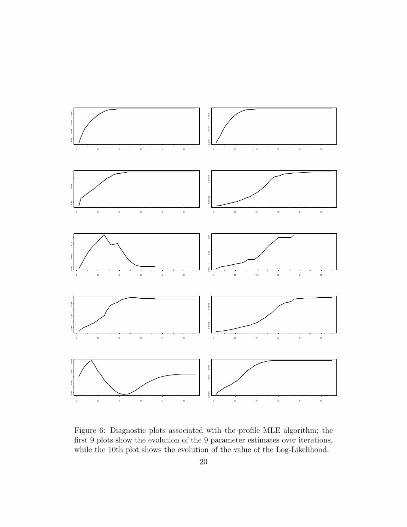
Figure 6 shows diagnostic plots associated with the DC–profile MLE algo-rithm. The first 9 plots show the evolution of the 9 parameter estimates overiterations; the 9 parameters are: a0, A, B, C for the IBM series; a0, A, B, C

15

0 500 1000 1500 2000

-0.2

-0.1

0.0

0.1

(i)

0 500 1000 1500 2000

-0.2

-0.1

0.0

0.1

(ii)

Figure 3: Daily returns from February 1, 1984 to December 31, 1991.(i) IBM stock returns. (ii) Hewlett-Packard stock returns.

16

0 10 20 30 40 50 60 70 80

-0.2

-0.1

0.0

0.1

(i)

0 10 20 30 40 50 60 70 80

-0.2

0-0

.10

0.0

(ii)

Figure 4: Daily returns from two months before to two months after thecrash of 1987. (i) IBM stock returns. (ii) Hewlett-Packard stock returns.

17

IBM

AC

F

0 5 10 15 20 25 30

0.0

0.2

0.4

0.6

0.8

1.0

IBM and HP

0 5 10 15 20 25 30

0.0

0.1

0.2

0.3

0.4

0.5

HP and IBM

Lag

AC

F

-30 -25 -20 -15 -10 -5 0

0.0

0.1

0.2

0.3

0.4

0.5

HP

Lag0 5 10 15 20 25 30

0.0

0.2

0.4

0.6

0.8

1.0

Multivariate Series : IBMvs.HP

Figure 5: Autocorrelation/cross-correlation plot of IBM vs. Hewlett-Packarddaily returns from February 1, 1984 to December 31, 1991.

18

for the H-P series, and ρ. Those 9 plots show convergence of the DC–profileMLE procedure; this is confirmed by the 10th plot that shows the evolutionof the value of the Log-Likelihood corresponding to those 9 parameters. Asexpected, the 10th plot shows an increasing graph that tapers off towards theright end, showing the maximization is working; only about 30-40 iterationsteps were required for convergence of the algorithm.

Finally, note that few people would doubt that a ρ value of 0.53, arisingfrom a dataset with sample size 2000, might not be significantly differentfrom zero; nonetheless, it is important to have a hypothesis testing procedurefor use in other, less clear, cases. A natural way to address this is via thesubsampling methodology—see Politis et al. (1999) for details. There aretwo complications, however:(i) Getting ρ is already quite computer-intensive, involving a numerical op-timization algorithm; subsampling entails re-calculating ρ over subsets (sub-series) of the data, and can thus be too computationally expensive.(ii) The estimators figuring in Tables 1 and 2 are not

√n–consistent as shown

in Hall and Yao (2003); subsampling with estimated rate of convergence couldthen be employed as in Ch. 8 of Politis et al. (1999).

Future work may focus on the above two important issues as well as onthe possibility of deriving likelihood-based standard errors and confidenceintervals in this non-standard setting.

References

[1] Bollerslev, T. (1986). Generalized autoregressive conditional het-eroscedasticity, Journal of Econometrics, 31, 307-327.

[2] Bollerslev, T. (1990). Modelling the coherence in short-run nominal ex-change rates: a multivariate generalized ARCH model, Review of Eco-nomics and Statistics, 72, 498-505.

[3] Bollerslev, T., Chou, R. and Kroner, K. (1992). ARCH modelling infinance: a review of theory and empirical evidence, Journal of Econo-metrics, 52, 5-60.

19

0 10 20 30 40 50

0.0

70.0

80.0

90.1

0

0 10 20 30 40 50

0.0

30

0.0

40

0.0

50

0 10 20 30 40 50

0.9

20.9

6

0 10 20 30 40 50

0.0

0002

0.0

0006

0 10 20 30 40 50

0.0

60.0

80.1

0

0 10 20 30 40 50

0.0

50.1

50.2

5

0 10 20 30 40 50

0.8

80.9

20.9

6

0 10 20 30 40 50

0.0

001

0.0

003

0 10 20 30 40 50

0.3

50.4

50.5

50.6

5

0 10 20 30 40 50

-20000

-5000

5000

Figure 6: Diagnostic plots associated with the profile MLE algorithm; thefirst 9 plots show the evolution of the 9 parameter estimates over iterations,while the 10th plot shows the evolution of the value of the Log-Likelihood.

20

[4] Bose, A. and Mukherjee, K. (2003), Estimating the ARCH parametersby solving linear equations, J. Time Ser. Anal., vol. 24, no. 2, pp. 127–136.

[5] Engle, R. (1982). Autoregressive conditional heteroscedasticity with es-timates of the variance of UK inflation, Econometrica, 50, 987-1008.

[6] Gourieroux, C. (1997). ARCH Models and Financial Applications,Springer Verlag, New York.

[7] Hall, P. and Yao, Q. (2003). Inference in ARCH and GARCH modelswith heavy-tailed errors, Econometrica, 71, 285-317.

[8] Patton, A.J. (2002). Skewness, asymmetric dependence and portfolios.Preprint (can be downloaded from: http://fmg.lse.ac.uk/∼patton).

[9] Politis, D.N. (2003), Model-free volatility prediction, Discussion Paper2003-16, Department of Economics, UCSD.

[10] Politis, D.N. (2004), A heavy-tailed distribution for ARCH residualswith application to volatility prediction, Annals of Economics and Fi-nance, 5, 283-298.

[11] Politis, D.N., Romano, J.P., and Wolf, M. (1999) Subsampling. Springer,New York.

[12] Shephard, N. (1996). Statistical aspects of ARCH and stochastic volatil-ity, in Time Series Models in Econometrics, Finance and Other Fields,D.R. Cox, David V. Hinkley and Ole E. Barndorff-Nielsen (eds.), Chap-man & Hall, London, pp. 1-67.

[13] Vrontos, I.D., Dellaportas, P. and Politis, D.N. (2003). A full-factormultivariate GARCH model, Econometrics Journal, 6, 312-334.

21