U.S. Department of the InteriorU.S. Geological Survey

Scientific Investigations Report 2005-5001

A Near-optimum Procedure for Selecting Stations in a Streamgaging Network

A Near-optimum Procedure for Selecting Stations in a Streamgaging Network

By Kenneth J. Lanfear

U.S. Geological Survey Scientific Investigations Report 2005-5001

U.S. Department of the InteriorU.S. Geological Survey

U.S. Department of the InteriorGale A. Norton, Secretary

U.S. Geological SurveyCharles G. Groat, Director

U.S. Geological Survey, Reston, Virginia: 2005

For more information about the USGS and its products: Telephone: 1-888-ASK-USGS World Wide Web: http://www.usgs.gov/

Any use of trade, product, or firm names in this publication is for descriptive purposes only and does not imply endorsement by the U.S. Government.

Although this report is in the public domain, permission must be secured from the individual copyright owners to reproduce any copyrighted materials contained within this report.

Suggested citation:Lanfear, K.J., 2005, A Near-optimum Procedure for Selecting Stations in a Streamgaging Network: Reston, Va., U.S. Geological Survey, Scientific Investigations Report 2005-5001, 10 p.

v

Contents

ABSTRACT …………………………………………………………………………………… 1Introduction …………………………………………………………………………………… 1

Federal Interests ………………………………………………………………………… 1Satisfying Goals ………………………………………………………………………… 2Finding Basic Feasible Incremental Solutions …………………………………………… 2Costs and Benefits ……………………………………………………………………… 3

Solution Algorithm …………………………………………………………………………… 3Alternative solution procedures ………………………………………………………… 3Initial Conditions ………………………………………………………………………… 4

Example Problem ……………………………………………………………………………… 4Data Sets ………………………………………………………………………………… 4Expert Rules for Selecting BFIS ………………………………………………………… 4Example Costs and Benefits …………………………………………………………… 5Determining the Example BFIS ………………………………………………………… 6Active Stations – Initial Conditions ……………………………………………………… 6Programming Implementation …………………………………………………………… 6Solution for All Goals …………………………………………………………………… 6Is the Solution Optimal? ………………………………………………………………… 7

Earlier Applications …………………………………………………………………………… 8Conclusions …………………………………………………………………………………… 8Literature Cited ……………………………………………………………………………… 8

TablesTable 1. Criteria for satisfying each type of Federal goal. …………………………………… 5Table 2. List of relative location costs assigned to solutions. ………………………………… 6Table 3. List of the number of goals of each type and the total number of BFIS’s that

satisfy each goal type. ……………………………………………………………… 6Table 4. Percent of each type of Federal goal satified by currently active stations. ………… 6Table 5. Example of how the algorithm can make a non-optimal choice. …………………… 8

FiguresFigure 1. Graph of the number of goals satisfied as a function of the number of stations

added. ……………………………………………………………………………… 7

Figure 2. Map of stations meeting example Federal goals. Active stations are shown in light gray and reactive stations in black. ………………………………………………… 8

ABSTRACTTwo questions are fundamental to Federal gov-

ernment goals for a network of streamgages which are operated by the U.S. Geological Survey: (1) how well does the present network of streamagag-ing stations meet defined Federal goals and (2) what is the optimum set of stations to add or reactivate to support remaining goals? The solution involves an incremental-stepping procedure that is based on Basic Feasible Incremental Solutions (BFIS’s) where each BFIS satisfies at least one Federal streamgaging goal. A set of minimum Federal goals for streamgaging is defined to include water mea-surements for legal compacts and decrees, flooding, water budgets, regionalization of streamflow char-acteristics, and water quality. Fully satisfying all these goals by using the assumptions outlined in this paper would require adding 887 new streamgaging stations to the U.S. Geological Survey network and reactivating an additional 857 stations that are cur-rently inactive.

IntroductionSince 1889, the U.S. Geological Survey (USGS)

has operated a streamgaging network to collect information about the Nation’s water resources. It is a multipurpose network funded by the USGS and many other Federal, State, and local agencies. Individual streamgaging stations are supported for specific purposes such as water allocation, reservoir operations, or regulating permit requirements, but the data are used for many other purposes. Thomas and Wahl (1993) surveyed cooperators and data users to identify uses of data in 9 categories. They found that uses of data from a typical streamgaging station fall into an average of 2.6 different data-use categories. The USGS recently examined the net-work to see how it is meeting Federal goals (U.S. Geological Survey, 1998). The evaluation defined key Federal goals for the network and established a set of quantitative metrics that measure the extent to which those goals are being achieved.

The evaluation technique in this report takes earlier analyses by the U.S. Geological Survey (1998; 1999) of how well the existing network meets goals to the next logical phase of determining how to improve the network by proposing an incre-mental-stepping procedure to select streamgaging stations that meet additional Federal goals. Key to

this technique is finding sets of stations or potential new station locations that efficiently meet indi-vidual goals. For any individual goal – for example, knowing the flow of a river at particular location – a limited number of practical configurations of stations can achieve the desired accuracy. By choos-ing from among limited sets of stations, rather than individual stations, we greatly reduce the number of possible solutions and ensure that the procedure will reach a near-optimum solution.

Federal Interests

Federal interests in streamgaging, which are defined in U.S. Geological Survey (1998; 1999), include supporting Federal programs, resolving disputes among states, and managing Federal lands. These broad interest categories were reduced to spe-cific types of Federal goals with quantitative mea-sures for determining success in meeting the goals. The list below includes important goals represen-tative of some major Federal interests. It does not represent a full compilation of Federal interests but is presented to demonstrate the analysis techniques.

• Compacts and Decrees—Streamflow data for interstate and international water transfers are required to satisfy legal compacts or court decrees.

• Flooding—The National Weather Service (NWS) provides forecasts of flooding condi-tions at 3,116 service locations on riverine systems where discharge measurements are required.

• Water Budget—Long-term, nationally con-sistent data on the inflows and outflows of major river basins plays a fundamental role in national water policies and planning. A goal, therefore, is to be able to provide estimates of the water budgets for each of the 329 river basins that cover the conterminous United States.

• Regionalization of Streamflow Characteris-tics—Ecoregions are based on perceived pat-terns of causal and integrative factors, includ-ing land use, land-surface form, potential natural vegetation, and soils (Omernik, 1987). Representative streams within each ecoregion need to be monitored to detect changes in streamflow that would result from changes in climate, changes in land-use practices,

2 A Near-optimum Procedure for Selecting Stations in a Streamgaging Network

or changes in ground-water withdrawals. The term “representative streams” refers to streams whose watershed lies entirely within the ecoregion, as opposed to streams that sim-ply flow through the ecoregion. 76 ecoregions cover the conterminous United States. Inter-secting the ecoregions with the polygons of 329 river basins leads to 802 ecoregion-basin combinations. Stations on representative streams in each of these areas would provide a network for detecting changes in streamflow and describing regional streamflow character-istics.

• Quality-Impaired Watersheds—The U.S. Environmental Protection Agency provided a list (Karen Klima, EPA, written communica-tion, January 26, 1999) of 533 watersheds (cataloging units) in which fewer than 50 per-cent of the assessed rivers meet State or tribal water-quality requirements for all designated uses.

• USGS Water-Quality Stations—Discharge measurements should complement mea-surements of a large suite of water-qual-ity parameters at National Stream Quality Accounting Network (NASQAN) stations (Ficke and Hawkinson, 1975), which are located primarily on major rivers; at Bench-mark stations (Lawrence, 1987), which are located primarily on streams unaffected by human influences; and at stations that are used by the National Water Quality Assess-ment (NAWQA) Program (Hirsch and others, 1988) for long-term, low-intensity sampling. These 3 sources comprise a total of 123 reaches.

Satisfying Goals

Represent N potential streamgaging stations with the N x 1 vector U, where each u

i equals 1

if station i is active and 0 if not active. Using the terminology of Yankowitz (1982), U

t is the “control

set” of the streamgaging network at stage t. Every stream reach can have one or more active or inactive stations, or is a candidate for a new station. Thus, there are at least as many possible station locations as there are reaches.

Let the M x 1 vector X represent the “state” of M goals. Each x

j represents a single goal. Exam-

ples of goals are: a NWS Service Location where streamflow must be determined; a basin for which inflow and outflow must be measured to deter-mine the water budget; a basin within an ecoregion

where at least one representative sampling station is required; or a long-term water-quality sampling location which requires estimates of streamflow. Let x

j equal 1 if the goal is met, 0 if it is not met. A goal

is either met or unmet; there is no partial satisfac-tion. Goals can be coincident. For example, a NWS Service Location might fall on an interstate cross-ing. Each, however, would be treated as a separate goal.

Define the “dynamics function,” f, which deter-mines if a goal is met, as equation 1:

xj = fj(U) . (1)

Each fj is determined by examining the net-

work and finding those stations or combinations of stations that would satisfy goal j. Assuming that every goal has at least one solution, then there exists at least one U

j such that f

j(U

j) equals 1. Now

impose another condition to eliminate solutions that contain redundant stations: discard a U

j if any

of its stations can be removed without its dynamics function becoming zero. A U

j that fulfils these two

conditions for any goal j is called a Basic Feasible Incremental Solution (BFIS). That is, a set of one or more stations (new, reactivated, or existing) that satisfies a goal, with all stations in the set being nec-essary to satisfy the goal, is a Basic Feasible Incre-mental Solution (BFIS) for that goal. A station can belong to more than one BFIS.

Finding Basic Feasible Incremental Solutions

Streamflow information commonly is estimated from nearby stations on the stream network; it is not necessary to have a streamgaging station exactly where you need to know the streamflow. Stations can be located upstream or downstream from the point of interest, and, in many cases, discharge values from multiple stations can be added or sub-tracted. Streamflow characteristics at ungaged sites can be estimated from regression analysis of nearby gaged sites (Moss and Karlinger, 1974, Moss and others, 1982, Moss and Tasker, 1991).

Determining an appropriate set of existing or new stations for estimating streamflow has been the subject of considerable research. Benson and Mata-las (1967) showed how basin characteristics could be used to estimate streamflow characteristics at ungaged sites. Stedenger and Tasker (1985) showed how generalized least squares could provide more accurate parameter estimates. Sharp (1971), looking to optimally place stations to measure the effects of known pollutant sources, developed a method for

SIR 2005-5001 3

selecting sampling locations based on the topol-ogy of the river network. Sanders and others (1983) applied a similar technique for allocating water-quality sampling stations. Karasev (1968) looked at minimum distance criteria.

With multiple objectives, no single method may suffice for selecting the BFIS. A goal of estimating regional streamflow parameters may require BFIS based on regression analysis. Selecting stations for a flood-warning goal would have to consider the stream network topology and travel times. More-over, any BFIS does not have to yield the most accurate estimate of streamflow; a BFIS need only provide sufficient accuracy to meet the purposes of the goal. The actual selection method for BFIS can be any combination of regression, analysis of stream network topology, examination of actual field conditions, or expert judgment.

Costs and Benefits

Let C be an N x 1 vector of costs associated with each station. Each c

i is the cost of activating

and operating station i. For any Ut,

Costt = C • Ut . (2)

For benefits, let W be an M x 1 vector repre-senting the benefits of each goal. Each w

j is the

benefit associated with fulfilling goal j. Then,

Benefitt = W • Xt = W • [fj(Ut)] . (3)

Solution AlgorithmA forward-stepping process adds one BFIS at a

time in an efficient manner to find a set of stations that satisfies all goals. The BFIS chosen in each step is that which provides the greatest ratio of incre-mental benefits to incremental cost.

The solution algorithm adds a BFIS in each step until there are no more goals to satisfy. Choose the optimal BFIS on the basis of its incremental cost because some of the stations in the BFIS may already have been added through other BFIS, and incremental benefits because a BFIS may happen to satisfy additional goals through common stations.

Let {B} be the set of all BFIS for all goals. The problem is to select a subset of {B} that optimally meets all goals. Starting with no selections, we will do this by adding one B

t at each stage, t, such that

each Bt fulfils at least one new goal. In calculating

benefits, we must account for all additional goals that B

t fulfils and assign the costs of any stations

needed to complete Bt that are not already in the

solution. The incremental costs and benefits of each stage are computed as follows.

For any Bt added,

Ut = Ut-1 ∪ Bt , (4)

∆Costt-(t-1) = C • (Ut – Ut-1) , (5)

and

∆Benefitt-(t-1) = W • (Xt – Xt-1) . (6)

In moving from stage t-1 to t, the gain, expressed as a benefit-cost ratio will be

Gt-(t-1) = ∆Benefitt-(t-1) / ∆Costt-(t-1) . (7)

The objective in each step is to select a Bk to

maximize the benefit-cost ratio of that step,

k | maxGt-(t-1) = W • ([fj(Ut-1 ∪ Bk)] – Xt-1) / C • ((Ut-1 ∪ Bk) – Ut-1) . (8)

This is where the BFIS play an important role. Since, by definition, each BFIS satisfies at least one goal, we are guaranteed that for some number of stages T where T ≤ M,

maxGt-(t-1) > 0 for t ≤ T (9)

and

maxGt-(t-1) = 0 for t > T . (10)

This ensures that the algorithm will proceed to a solution that satisfies all goals.

Alternative solution procedures

A simpler procedure for selecting an appro-priate solution might be to add one station per step, rather than one BFIS. Maddock (1974) used a technique of removing stations one-by-one in looking at how to reduce the number of stations in a network. Tasker (1986) used a backward-step-ping technique to select stations that minimized the average sampling mean-square error of a regional regression equation. The problem with adding one station per step is that, at some step, all remaining goals might require two or more stations each.

4 A Near-optimum Procedure for Selecting Stations in a Streamgaging Network

This will set all incremental benefit-cost ratios maxGt-(t-1) equal to zero before all the goals are satisfied, which will cause the algorithm to stall before it achieves a solution. Tasker (1986) did not face this problem because he considered a single goal involving regional regression. A way around this local minimum is an n-step algorithm – that is, trying all combinations of N stations. This method, however, becomes computationally infeasible with a large number of stations. Selecting from among the BFIS, as proposed here, effectively implements an n-step technique with a variable n being the number of stations in each BFIS.

Another variant would be to allow partial goal solutions. That is, allow f to take on any real num-ber 0 ≤ f ≤ 1. While this eliminates the problem of stalling at local minima, it introduces the possibility of selecting stations that ultimately don’t contribute to satisfying a goal. A solution that is not a union of BFIS’s can not be optimal since it will include sta-tions that contribute nothing to the solution.

The solution can not be solved by linear pro-gramming because the BFIS can share stations and, thus, are not independent of each other. Fier-ing (1965) used nonlinear integer programming to decide which sites in a network should be gaged further. His approach bears many similarities to the one proposed here, but it is based on individual sta-tions, not sets of stations.

Burn and Goulter (1991) and Yang and Burn (1994) used clustering techniques to identify groups of similar stations, then selected a single station from each group. Their method is applicable to regionalization, but does not address the problem of multiple goals.

Initial Conditions

One set of initial conditions is to accept the currently active stations as a given. Goals satisfied by the set of active stations are eliminated from the solution before beginning the iteration procedure. Depending on how successful the active stations are in meeting the goals, this approach can substantially reduce the computation time for selecting BFIS to satisfy the remaining goals. Of course, the selected set of stations will be optimized only for the added goals, not the entire set of goals.

Example Problem

Data Sets

An analysis of this scope would not be possible without a substantial infrastructure of geospatial data sets:

• Traces of 60,000 stream segments that consti-tute 1 million kilometers of rivers. Attributes of the reaches include information on how the reaches connect to each other, so that the net-work can be traced upstream or downstream.

• Locations of 17,823 active and historical USGS streamgaging stations within the con-terminous United States. About 6,600 stations were active in 1996; each station is related to a stream reach.

• Locations of 3,116 National Weather Service locations where flood forecasts are provided for riverine systems. Each location is related to a stream reach, and about two-thirds are related to a specific USGS streamgaging sta-tion.

• Boundaries of 329 river basins (accounting units) and 2,079 watersheds (cataloging units) in the conterminous United States.

• Boundaries of 76 ecoregions (Omernik, 1987) in the conterminous United States.

Expert Rules for Selecting BFIS

Many hydrologic judgments can be expressed as rules that apply to a network of streams as repre-sented by a GIS. Rules for finding sets of BFIS can address:

• Percent of the basin that must be gaged. That is, what percent of the target basin must be gaged by stations upstream, or what percent additional area may be added by using sta-tions downstream;

• How far away in stream distance a station may be located upstream or downstream;

• The number of stations and the sizes of their drainage areas;

• Whether stations upstream or downstream of reservoirs may be used;

• Whether stations on large mainstem rivers

SIR 2005-5001 5

may be included; or

• Whether requirements such as satisfying legal compacts require an exact match to an exist-ing USGS streamgaging station.

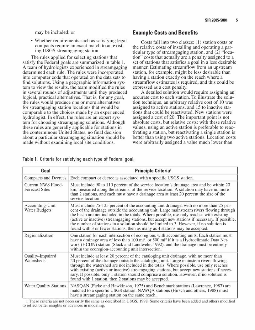
The rules applied for selecting stations that satisfy the Federal goals are summarized in table 1. A team of hydrologists experienced in streamgaging determined each rule. The rules were incorporated into computer code that operated on the data sets to find solutions. Using a geographic information sys-tem to view the results, the team modified the rules in several rounds of adjustments until they produced logical, practical alternatives. That is, for any goal, the rules would produce one or more alternatives for streamgaging station locations that would be comparable to the choices made by an experienced hydrologist. In effect, the rules are an expert sys-tem for choosing streamgaging solutions. Although these rules are generally applicable for stations in the conterminous United States, no final decision about a particular streamgaging situation should be made without examining local site conditions.

Example Costs and Benefits

Costs fall into two classes: (1) station costs or the relative costs of installing and operating a par-ticular type of streamgaging station, and (2) “loca-tion” costs that actually are a penalty assigned to a set of stations that satisfies a goal in a less desirable manner. Estimating streamflow from an upstream station, for example, might be less desirable than having a station exactly on the reach where a streamflow estimates is required, and this could be expressed as a cost penalty.

A detailed solution would require assigning an accurate cost to each station. To illustrate the solu-tion technique, an arbitrary relative cost of 10 was assigned to active stations, and 15 to inactive sta-tions that could be reactivated. New stations were assigned a cost of 20. The important point is not absolute costs, but relative costs: with these relative values, using an active station is preferable to reac-tivating a station, but reactivating a single station is better than using two active stations. Location costs were arbitrarily assigned a value much lower than

Table 1. Criteria for satisfying each type of Federal goal.

Goal Principle Criteria1

Compacts and Decrees Each compact or decree is associated with a specific USGS station.

Current NWS Flood-Forecast Sites

Must include 90 to 110 percent of the service location’s drainage area and be within 20 km, measured along the streams, of the service location. A solution may have no more than 2 stations, and each must have a drainage area at least 20 percent the size of the service location.

Accounting-Unit Water Budgets

Must include 75-125 percent of the accounting unit drainage, with no more than 25 per-cent of the drainage outside the accounting unit. Large mainstream rivers flowing through the basin are not included in the totals. Where possible, use only reaches with existing (active or inactive) streamgaging stations, but accept new stations if necessary. If possible, the number of stations in a solution should be limited to 3. However, if no solution is found with 3 or fewer stations, then as many as 4 stations may be accepted.

Regionalization One station for each intersection of ecoregions with accounting units. Each station must have a drainage area of less than 100 mi2, or 500 mi2 if it is a Hydroclimatic Data Net-work (HCDN) station (Slack and Landwehr, 1992), and the drainage must be entirely within the ecoregion-accounting unit intersection.

Quality-Impaired Watersheds

Must include at least 20 percent of the cataloging unit drainage, with no more than 20 percent of the drainage outside the cataloging unit. Large mainstem rivers flowing through the watershed are not included in the totals. Where possible, use only reaches with existing (active or inactive) streamgaging stations, but accept new stations if neces-sary. If possible, only 1 station should comprise a solution. However, if no solution is found with 1 station, then 2 stations may be accepted.

Water Quality Stations NASQAN (Ficke and Hawkinson, 1975) and Benchmark stations (Lawrence, 1987) are matched to a specific USGS station. NAWQA stations (Hirsch and others, 1988) must have a streamgaging station on the same reach.

1 These criteria are not necessarily the same as described in USGS, 1998. Some criteria have been added and others modified to reflect better insights or advances in modeling.

6 A Near-optimum Procedure for Selecting Stations in a Streamgaging Network

that of station costs, so that the location cost broke ties among solutions having equal station costs. The location cost depended upon the placement of stations relative to the goal that needs to be satisfied (table 2).

Table 2. List of relative location costs assigned to solutions.

Location of solution Location cost

Exact match to USGS station required by the goal

0.0

On the same reach as the goal requires 0.1

One or more stations upstream of the reach the goal requires

0.2

One or more stations downstream of the reach the goal requires

0.3

For a regionalization goal, the station is not an HCDN station (Slack and Landwehr, 1992)

0.1

Because the intent of this example run was to satisfy all goals, the goals were assigned equal benefits by making W the unit vector. This way, the algorithm is free to pick the BFIS in any way that minimizes the cost of the stations required.

The analysis tool was used to examine how the set of USGS streamgaging stations that were active in 1996 met each of the Federal goals. Then, starting over with no stations selected, BFIS’s were chosen to fully meet all the goals. Remember that this analysis uses only streamgaging stations oper-ated by the USGS. There are hundreds of additional streamgaging stations operated by local, State, and other Federal agencies. Although these non-USGS streamgaging stations are not included in this study, the USGS plans to incorporate their contribution to the defined Federal streamgaging goals when data on their locations are compiled.

Determining the Example BFIS

Examining each of the goals yielded a total of 20,865 BFIS’s (table 3). The number of BFIS per goal varies widely and depends on how many ways a goal can be satisfied. Only a single specified sta-tion can satisfy some goals, such as Compacts and Decrees. Many different combinations can satisfy others.

Table 3. List of the number of goals of each type and the total number of BFIS’s that satisfy each goal type.

Goal type No. of goals

No. of BFIS

Compacts and Decrees 120 120

Flooding 3,116 10,469

Water Budget 329 3,983

Regionalization 802 4,231

Quality-Impaired Watersheds 533 1,902

Water Quality Stations 123 160

TOTAL 5,023 20,865

Active Stations – Initial Conditions

Currently active stations achieved the levels of goal satisfaction shown in table 4.

Table 4. Percent of each type of Federal goal satis-fied by currently active stations.

Goal type Percent SatisfiedCompacts and Decrees 100%

Flooding 66%

Water Budget 57%

Regionalization 58%

Quality-Impaired Watersheds 71%

Water Quality Stations 81%

Programming Implementation

Determining the BFIS and solving the optimiza-tion problem were implemented in software using the Perl programming language (Wall and others, 1996). Perl was chosen because its complex data structures could easily represent stream network topology and the relationship of the BFIS to the individual stations. It would be possible to accom-plish the same thing with many other languages. The programs were used to solve a very specific problem and were not written in a generalized form for widespread distribution.

Solution for All Goals

Starting the analysis with no stations selected and continuing until all Federal goals listed herein are satisfied, 2,313 active stations, 857 reactivated stations and 887 new stations would be required, for

SIR 2005-5001 7

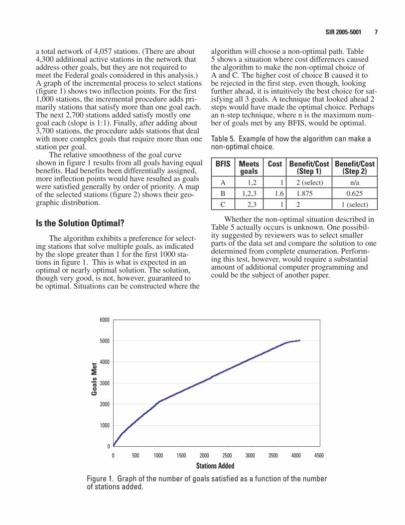
a total network of 4,057 stations. (There are about 4,300 additional active stations in the network that address other goals, but they are not required to meet the Federal goals considered in this analysis.) A graph of the incremental process to select stations (figure 1) shows two inflection points. For the first 1,000 stations, the incremental procedure adds pri-marily stations that satisfy more than one goal each. The next 2,700 stations added satisfy mostly one goal each (slope is 1:1). Finally, after adding about 3,700 stations, the procedure adds stations that deal with more complex goals that require more than one station per goal.

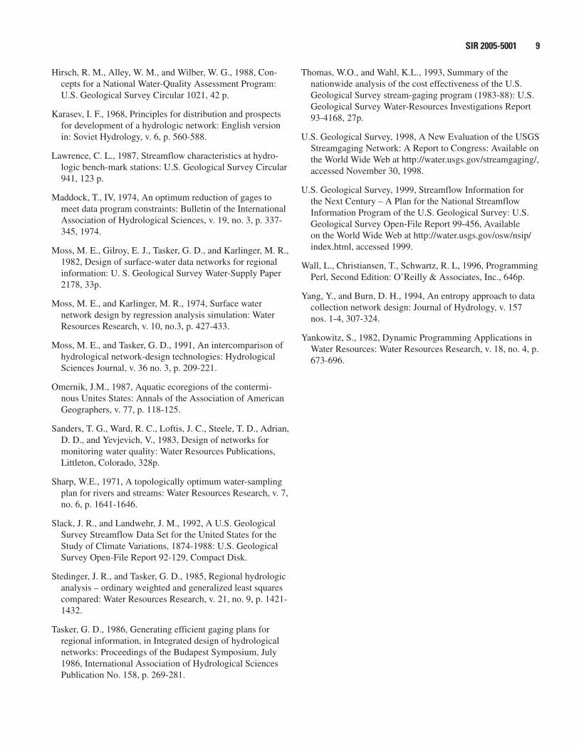
The relative smoothness of the goal curve shown in figure 1 results from all goals having equal benefits. Had benefits been differentially assigned, more inflection points would have resulted as goals were satisfied generally by order of priority. A map of the selected stations (figure 2) shows their geo-graphic distribution.

Is the Solution Optimal?

The algorithm exhibits a preference for select-ing stations that solve multiple goals, as indicated by the slope greater than 1 for the first 1000 sta-tions in figure 1. This is what is expected in an optimal or nearly optimal solution. The solution, though very good, is not, however, guaranteed to be optimal. Situations can be constructed where the

algorithm will choose a non-optimal path. Table 5 shows a situation where cost differences caused the algorithm to make the non-optimal choice of A and C. The higher cost of choice B caused it to be rejected in the first step, even though, looking further ahead, it is intuitively the best choice for sat-isfying all 3 goals. A technique that looked ahead 2 steps would have made the optimal choice. Perhaps an n-step technique, where n is the maximum num-ber of goals met by any BFIS, would be optimal.

Table 5. Example of how the algorithm can make a non-optimal choice.

BFIS Meets goals

Cost Benefit/Cost (Step 1)

Benefit/Cost (Step 2)

A 1,2 1 2 (select) n/a

B 1,2,3 1.6 1.875 0.625

C 2,3 1 2 1 (select)

Whether the non-optimal situation described in Table 5 actually occurs is unknown. One possibil-ity suggested by reviewers was to select smaller parts of the data set and compare the solution to one determined from complete enumeration. Perform-ing this test, however, would require a substantial amount of additional computer programming and could be the subject of another paper.

Figure 1. Graph of the number of goals satisfied as a function of the number of stations added.

0

1000

2000

3000

4000

5000

6000

0 500 1000 1500 2000 2500 3000 3500 4000 4500

Stations Added

Goa

ls M

et

8 A Near-optimum Procedure for Selecting Stations in a Streamgaging Network

Earlier ApplicationsThe example shown in this paper should only

be regarded as a starting point for discussions, as other reasonable assumptions about goals and costs could be made. In 1998, the U.S. Geological Survey (1998), for example, employed an earlier version of this technique to evaluate how well the existing streamgaging network met selected Federal goals. However, the study was based upon preliminary data, a few different goals, and slightly different rules for satisfying goals and determining solu-tions. In 1999, the U.S. Geological Survey (1999) employed this technique as a starting point, but made simplifying assumptions about goals for water quality and long-term change detection.

ConclusionsThis paper describes and demonstrates an

incremental technique for selecting a nearly opti-mal set of streamgaging stations to meet any given set of goals for streamflow information, such as flood protection, water allocations, water quality, and long-term changes. Data sets are available that have adequate resolution to apply this technique on a scale suitable for the conterminous United States for Federal goals concerning: compacts and decrees; flooding; water budgets; regionalization of streamflow characteristics; quality-impaired watersheds; and USGS water-quality stations. The

technique is sufficiently scalable to deal success-fully with the entire network of USGS streamgag-ing stations.

A preliminary model run indicates that add-ing 887 new streamgaging stations and reactivating 857 others could meet some of the most important Federal goals for streamgaging in the contermi-nous United States. This should only be regarded as a starting point for discussions, as other reason-able assumptions about goals and costs could be made. The analysis technique provides a tool for quantitatively evaluating the number and location of streamgaging stations for any list of Federal streamgaging goals, now, or in a future time with different priorities.

Literature Cited

Benson, M. A., and Matalas, N. C., 1967, Synthetic hydrology based on regional statistical parameters: Water Resources Research, v. 3, no. 4, p, 931-935.

Burn, D. H., and Goulter, I.C., 1991, An approach to the ratio-nalization of streamflow data collection networks: Journal of Hydrology, v. 122, p. 71-91.

Ficke, J. F., and Hawkinson, R. O., 1975, The National Stream Quality Accounting Network (NASQAN) – Some questions and answers: U.S. Geological Survey Circular 719, 23 p.

Fiering, M. B., 1965, An optimization scheme for gaging: Water Resources Research, v. 1, no. 4, p. 463-470.

Figure 2. Map of stations meeting example Federal goals. Active stations are shown in light gray and reactive stations in black.

SIR 2005-5001 9

Hirsch, R. M., Alley, W. M., and Wilber, W. G., 1988, Con-cepts for a National Water-Quality Assessment Program: U.S. Geological Survey Circular 1021, 42 p.

Karasev, I. F., 1968, Principles for distribution and prospects for development of a hydrologic network: English version in: Soviet Hydrology, v. 6, p. 560-588.

Lawrence, C. L., 1987, Streamflow characteristics at hydro-logic bench-mark stations: U.S. Geological Survey Circular 941, 123 p.

Maddock, T., IV, 1974, An optimum reduction of gages to meet data program constraints: Bulletin of the International Association of Hydrological Sciences, v. 19, no. 3, p. 337-345, 1974.

Moss, M. E., Gilroy, E. J., Tasker, G. D., and Karlinger, M. R., 1982, Design of surface-water data networks for regional information: U. S. Geological Survey Water-Supply Paper 2178, 33p.

Moss, M. E., and Karlinger, M. R., 1974, Surface water network design by regression analysis simulation: Water Resources Research, v. 10, no.3, p. 427-433.

Moss, M. E., and Tasker, G. D., 1991, An intercomparison of hydrological network-design technologies: Hydrological Sciences Journal, v. 36 no. 3, p. 209-221.

Omernik, J.M., 1987, Aquatic ecoregions of the contermi-nous Unites States: Annals of the Association of American Geographers, v. 77, p. 118-125.

Sanders, T. G., Ward, R. C., Loftis, J. C., Steele, T. D., Adrian, D. D., and Yevjevich, V., 1983, Design of networks for monitoring water quality: Water Resources Publications, Littleton, Colorado, 328p.

Sharp, W.E., 1971, A topologically optimum water-sampling plan for rivers and streams: Water Resources Research, v. 7, no. 6, p. 1641-1646.

Slack, J. R., and Landwehr, J. M., 1992, A U.S. Geological Survey Streamflow Data Set for the United States for the Study of Climate Variations, 1874-1988: U.S. Geological Survey Open-File Report 92-129, Compact Disk.

Stedinger, J. R., and Tasker, G. D., 1985, Regional hydrologic analysis – ordinary weighted and generalized least squares compared: Water Resources Research, v. 21, no. 9, p. 1421-1432.

Tasker, G. D., 1986, Generating efficient gaging plans for regional information, in Integrated design of hydrological networks: Proceedings of the Budapest Symposium, July 1986, International Association of Hydrological Sciences Publication No. 158, p. 269-281.

Thomas, W.O., and Wahl, K.L., 1993, Summary of the nationwide analysis of the cost effectiveness of the U.S. Geological Survey stream-gaging program (1983-88): U.S. Geological Survey Water-Resources Investigations Report 93-4168, 27p.

U.S. Geological Survey, 1998, A New Evaluation of the USGS Streamgaging Network: A Report to Congress: Available on the World Wide Web at http://water.usgs.gov/streamgaging/, accessed November 30, 1998.

U.S. Geological Survey, 1999, Streamflow Information for the Next Century – A Plan for the National Streamflow Information Program of the U.S. Geological Survey: U.S. Geological Survey Open-File Report 99-456, Available on the World Wide Web at http://water.usgs.gov/osw/nsip/index.html, accessed 1999.

Wall, L., Christiansen, T., Schwartz, R. L, 1996, Programming Perl, Second Edition: O’Reilly & Associates, Inc., 646p.

Yang, Y., and Burn, D. H., 1994, An entropy approach to data collection network design: Journal of Hydrology, v. 157 nos. 1-4, 307-324.

Yankowitz, S., 1982, Dynamic Programming Applications in Water Resources: Water Resources Research, v. 18, no. 4, p. 673-696.