a network fire model for the simulation of fire growth and

A Network Fire Model for the Simulationof Fire Growth and Smoke Spreadin Multiple Compartments with

Complex Ventilation

JASON E. FLOYD* AND SEAN P. HUNT

Hughes Associates, Inc., 3610 Commerce Dr., Suite 817,Baltimore, MD 21227-1652, USA

FRED W. WILLIAMS

Naval Technology Center for Safety and SurvivabilityChemistry Division, Naval Research Laboratory,

Washington DC, USA

PATRICIA A. TATEM

ITT Industries Advanced Engineering and Sciences DivisionAlexandria, Virginia, USA

ABSTRACT: There is a need for fire modeling tools capable of rapid simulationof fire growth and smoke spread in multiple compartments with complex ventilation.Currently available tools are not capable of simulation of complex ventilationarrangements in a timely manner. To address this problem, a new fire modelcalled Fire and Smoke SIMulator (FSSIM) has been developed. FSSIM is a networkmodel whose core thermal hydraulic routines are based on MELCOR. FSSIMcapabilities include remote ignition, multilayer heat conduction, radiation streaming,arbitrarily complex HVAC systems, detection, suppression, oxygen-limited combus-tion, and simple control systems.

KEY WORDS: computer model, fire, smoke, multiple compartments, HVAC.

*Author to whom corresponence should be addressed. E-mail: [email protected]

Journal of FIRE PROTECTION ENGINEERING, Vol. 15—August 2005 199

1042-3915/05/03 0199–31 $10.00/0 DOI: 10.1177/1042391505051358� 2005 Society of Fire Protection Engineers

INTRODUCTION

ANEW FIRE model has been developed for simulating fire growthand smoke spread onboard naval vessels [1]. The core physics models

are not naval specific [2]; therefore, the model is also applicable insimulating any multiple compartment enclosure. This article provides anoverview of the model’s core algorithms as well as shows some validationusing experimental data collected from a set of single compartment fire testdata and from fire testing onboard the Navy’s fire test platform, the ex-USSShadwell [3].

Motivation

The impetus for developing a network fire model arose from currentneeds of the design process for future surface combatants [4]. Fire representsa significant threat to a ship both in terms of its impact on crew health andequipment. Fire growth and spread onboard a combatant can quickly resultin a loss of mission capability. Furthermore, the presence of large quantitiesof flammable liquids, missile propellants, and explosives onboard a typicalcombatant greatly increases the risk that a fire represents.

As part of the design process for future combatants, candidate designsmust demonstrate that they meet specific requirements for maintain-ing fighting capability after a weapon hit. This is done by simulatingthe ship’s response to a large number, hundreds to thousands, of scenarios.In addition, this simulation must account for the total ship response,which for an aircraft carrier can involve thousands of compartments.The simulation process includes accounting for direct damage from theweapon, cascading failures that result from progressive fire spreadand flooding, and the damage control response of automated systemsand the crew. As the designs continuously evolve, analysis needs to be rapidso that any lessons learned can be meaningfully applied to the designevolution.

Currently available computational tools do not support this process.Computational fluid dynamics (CFD), while quite capable in simulating theeffects of fire, do not support rapid analysis in a cost-effective manner.Heuristic methods, rules or correlation based, while rapid, tend to be overlyconservative. Existing zone models, while rapid, lack the ability to modelcontrol systems, have limitations in the complexity of ventilation systems,and were not designed for integration as a federate in a simulationenvironment. Thus, in order to meet the needs of the design process, thedecision was made to develop a new fire model. To maximize speed,a network model approach was used.

200 J. E. FLOYD ET AL.

Network Model

In the realm of computational heat and mass transfer, a network modelrepresents the lowest level of abstraction for a multiple volume prototype.In a network model, each control volume of interest is represented as a singlenode. In some sense, this could be referred to as a one-zone model. For thepurposes of the model in this article, a control volume is either acompartment or a heating, ventilation and air conditioning (HVAC)system component, where multiple ducts connect, for example, a tee orplenum. Heat and mass transfer occur by defining junctions between nodes.These junctions represent flow paths for the transfer of information betweennodes. In the case of a flow solver, the information is mass, energy, andmomentum. With one node per control volume, a network model minimizesthe size of the computational space required for flow solution. This is animportant consideration for a surface combatant, which has hundreds ofcompartments with multiple flow connections in the form of doors, hatches,and HVAC systems. A schematic diagram of the network model conceptis shown in Figure 1.

A survey of existing network models for multiple compartmentcapabilities did not uncover an existing tool with the desired functionality.A few of these tools and their limitations are identified here. Note that noneof these tools are currently designed to operate as a federate within asimulation environment.

. CFAST – CFAST is a widely used and well-validated zone model [8].It does have many of the desired capabilities. However, CFAST’s firespread capabilities require the definition of specific objects within a spacethat are heated by gas phase interactions as opposed to surface contactwhich is a primary method of spread onboard a ship. CFAST does notallow for time-dependent flow areas for vertical flow openings. CFAST isknown to have stability problems for large computations, and an entireship simulation will have hundreds to thousands of compartments withnumerous ventilation systems.

. CONTAM – CONTAM is an HVAC network model developed by theNational Institute of Standards and Technology [5]. While CONTAMhas numerous features supporting the computation of buoyant flows andHVAC system flows within a building, it does not contain any models forcombustion-related phenomena. It also does not contain models forsurface heat transfer.

. FIRAC – FIRAC was developed by Los Alamos National Laboratories,for the purpose of predicting the dispersion of radionuclides through acomplex ventilation system [6]. Only a single fire can be specified in

A Network Fire Model 201

FIRAC, as its intent was to examine a single accident scenario such as afire in a glove box. As its ultimate goal was to predict the radioactivesource term, the model does not include suppression and detection, firespread, and compartment-to-compartment heat transfer.

. MELCOR – MELCOR is a US Nuclear Regulatory Commissionsoftware tool for simulating the post accident response of reactor con-tainment systems [2]. It is a network model with multiphase, multifluidcapabilities as well as surface heat transfer models. MELCOR, however,does not contain any combustion, detection, or suppression modelsbeyond a model for hydrogen deflagration.

Fire and Smoke SIMulator (FSSIM)

Fire and Smoke SIMulator [1] is written in standard FORTRAN 95.It runs on both Windows and Linux platforms. FSSIM uses a Fortran

Five heat transferconnections to theambient

Four heat transferconnections to theambient

Five heat transferconnections to theambient

One heat transferconnection andone bidirectionaljunction

One heat transferconnection andone bidirectionaljunction

Three ducts andone node

One fan

One fire

Figure 1. Network model concept. (The color version of this figure is available on-line.)


namelist format for its input file, the same method of input used by FireDynamics Simulator (FDS) [7]. FSSIM has the following capabilities:

. 1-D flow model including friction losses and temperature-dependentspecific heat.

. 1-D multiple layer, temperature-dependent heat transfer.

. N-surface, gray-gas radiation heat transfer, including radiation streamingthrough openings.

. Bidirectional flow through horizontal (hatches) and vertical (doors) flowconnections.

. Combustion product species tracking.

. Oxygen- and fuel-limited combustion.

. Multiple user-defined fires along with fire spread via compartment-to-compartment heat transfer.

. HVAC systems including ducts, dampers, and fans with forward andreverse flow losses and multiple fan models.

. Fire detection via heat, smoke, and flame detection

. Fire spread by compartment-specific criteria.

. Fire suppression via sprinklers, water mist, gaseous agents, aerosolagents, and foam.

. Fire spread prevention via boundary cooling.

. Simple control systems to link operation of equipment to sensors ortimes.

. Surface leakage.

. Fast, order-real-time execution speed.

There is no practical limit other than time and available resources tothe number of compartments, surfaces, vent connections, or the complexityof HVAC systems. Output from FSSIM consists of a series of comma-separated value (csv) files. The user can select groups of parameters foroutput, for example, compartment temperature or junction velocity, andany single parameter will be written to multiple csv files, if more than 255columns is required, a number consistent with current csv file import limitsin Microsoft Excel�.

The overall FSSIM solver is based on the MELCOR [2] thermal hydraulicsolver. MELCOR is a US Nuclear Regulatory Commission softwarepackage for performing nuclear power plant containment safety analyses.MELCOR contains a number of submodels including heat and masstransfer, spray cooling systems, deflagrations, and molten core–concreteinteractions. FSSIM also includes a radiation heat transfer model based onCFAST’s model [8] and a 1-D finite difference heat conduction modelsimilar to that found in HEATING [9]. In this article, only the primaryalgorithms for heat and mass transfer are addressed.


Hydraulic Model

The FSSIM hydraulic solver solves the 1-D conservation equations formass, momentum, and energy. Energy and mass are conserved explicitly;whereas, momentum is conserved implicitly. Energy conservation and massconservation use a control volume approach, where the control volumeis either a single compartment or a ventilation system node. Momentum isimplicitly solved for in vent connections or in ducts.

Mass:

dMi

dt¼Xj

�ij�dj vjFjAj þ _MMi ð1Þ

Energy:

dEi

dt¼Xj

�ijvjFjAj�dj h

dj þ

_EEi ð2Þ

Momentum:

�jLjdvj

dt¼ Pi � Pkð Þ þ �g�zð Þjþ�Pj �

1

2Kj�j vj

�� vj ð3Þ

Equation of State:

PiVi ¼R

mwair

Ei

cpi Tið Þð4Þ

In the above equations, i and k indicate a node (compartment or HVACduct endpoint) and j indicates a single junction (doorway, hatch, or lengthof duct), note two compartments may be joined by multiple junctions. Theterm � is a direction indicator, where a positive flow is defined as one exitingthe compartment, d indicates a donor or upwind quantity, A represents themaximum flow of a junction, and F is the fraction of the flow area availableand is utilized for time-dependent junction areas, for example, opening orclosing a door. The mass and energy equations differ slightly for a duct nodeversus a compartment node. The FSSIM HVAC model assumes no mass orenergy storage in an HVAC system. Thus, at any node in the system, massand energy in must equal mass and energy out. Therefore, for a duct node,the time derivatives of mass and energy are zero.


The momentum equation is solved implicitly (details to be discussed later)and the mass and energy equations are solved explicitly. Hence, mass andenergy will be conserved; however, momentum may not be. Since the flowfields are highly abstracted in a lumped-parameter model, many con-tributors to the momentum are not being captured. On the other hand, it iscritical to account for toxic combustion products or the energy release fromcombustion.

In general, donor or upwind quantities are used in the solution. Theexception is the density term in the momentum equation, where an iteration-dependent density formulation is used. If the combined pressure andbuoyancy gradients are small, a change in flow direction may occur whileiterating the solver. This would result in a change in the donor density,which could result in further flow oscillation. To ensure convergence in sucha situation, the momentum density used is:

�nþ1j ¼ ��nj þ 1� �ð Þ�dj , ð5Þ

where, � is an iteration-dependent value from 0 to 1, d indicates a donorquantity, and n is the inner iteration number. For the first third of theallowed number of inner iterations, �¼ 0, and a pure donor value is used fordensity. For the second third, � is varied linearly from 0 to 1. For the lastthird, �¼ 1, and the density is fixed to the value at the prior iteration. Sinceflow oscillations can occur only if the combined pressure and buoyancygradients across a junction are small, this typically occurs if either thedensities are similar or the velocity is small. In either case, the impact offixing the density on the solution is minimal.

The mass, energy, and momentum equations are differenced using anexplicit Euler time step for mass and energy and a semiimplicit time step formomentum. The friction term in the momentum equation is approximatedusing a tangent/secant approach [2] to aid convergence when flow directionchanges. The differenced equations as used in FSSIM are provided here.

Mass:

Mni ¼

Xj

�ij�dj v

nj F

njAj þ _MMn

i

!�t n þMn�1

i ð6Þ

Energy:

E ni ¼

Xj

�ijvnjF n

jAj�

dj h

djþ _EE n

i

!�t n þ E n�1

i ð7Þ


Momentum:

vnj 1þKj�tn

2Ljvn�j �vnþ��

��tn

2

�jLj

R

mwair

�1

Vicnþpi

Xj1 connected to i

�j1�dj1Aj1F

nj1v

nj1h

dj1�

1

Vkcnþpk

Xj2 connected to k

�j2�dj2Aj2F

nj2v

nj2h

dj2

!

¼ vn�1j þ

�tn

�jLj

Pn�1i

cn�picnþpi

þ _qqiR

mwairVicnþpi�Pn�1

k

cn�pkcnþpk

� _qqkR

mwairVkcnþpk

þ�Pjþ �g�zð Þn�1j

!þKj�tn

2Ljvnþj

�� vn�j� �ð8Þ

The momentum equation is sufficiently complex to warrant explanation.The velocity at the next time step is determined by the average pressuredifference across a junction which is computed using the compartment staticpressure gradient and the junction endpoint elevations in compartments iand j. The pressure in the compartment is a function of the mass and energyflows in and out of the compartment. Thus, the velocity through a givenjunction is a function of the pressures in all of the compartments directlyconnected to the junction’s endpoints through other junctions. Hence, thetwo summation terms in Equation (8), which account for the energy flows inthe source and destination compartments. The friction term in Equation (3)was discretized as follows:

1

2Kj�j vj

�� vj ! Kj�tn

2Ljvn�j � vnþ�� vnj � vnþj

�� vn�j� �ð9Þ

where n� is the prior iteration velocity, n is the next time step velocity, andnþ is the current guess for velocity. nþ will be the prior iteration valueif flow direction remains constant, and it will be zero if the flow directionchanges between iterations. The term �g�zð Þ is the buoyancy head, which isdefined as:

�g�zð Þj¼ �k � �ið Þ zj þ1

2�zj

� �þ �i zi þ

1

2�zi

� �� k zk þ

1

2�zk

� �� g

ð10Þ

Fire and Smoke SIMulator allows for bidirectional flow in both vertical(doors) and horizontal (hatches) flow connections. As mentioned earlier,


HVAC duct flows are assumed to be unidirectional. For bidirectional flowjunctions, each junction is treated internally as two parallel junctions. For adoorway, the junction is partitioned according to the location of the neutralplane at the start of each time step. To avoid instabilities in the solver, thechange in junction area between time steps is relaxed and no paralleljunction is allowed to be <1% of the available flow area. Thus, it is possiblethat both portions of the junction may have the same flow direction. Fora horizontal junction, the method of Cooper is used [10]. In this approach,a flooding criterion is computed for the junction. If the pressure gradientexceeds the flooding criterion, then unidirectional flow occurs. If thepressure gradient is less than the flooding criterion, bidirectional flowoccurs. The momentum equation for flow in the direction indicated by thecurrent pressure and density gradients, for example, as would occurassuming unidirectional flow, is modified to replace vj with vjþ vj,ex, where,vj,ex is an exchange flow. A correlation-based momentum equation is thenused for vj,ex:

v nj, ex þKj

2Ljv n�j, ex � vnþj, ex

�� v nj, ex ¼ v n�1j, ex þ �j, ex

�tn

Lj

1

2Kj

� 0:0554F n

j Aj

�

ffiffiffiffiffiffiffiffiffiffiffiffiffiffiffiffiffiffiffiffiffiffiffiffi8g��jF n

j Aj

� �i þ �kð Þ

s1�

�Pj

�� Pj, flood

�� !0

@1A

2

þKj�tn

2Ljv nþj, ex

�� v n�j, ex ð11Þ

Heat Transfer

Fire and Smoke SIMulator heat transfer sub-models include correlation-based convection heat transfer; N-surface, gray gas, radiation heat transfer;and 1-D, multilayer, temperature-dependent conduction. A compartmentcan have as many surfaces as required to define its heat conduction paths;for example, if a compartment is adjacent to three compartments along onewall, three surfaces can be defined for that wall.

Conduction

The general equation for 1-D heat transfer in Cartesian coordinates is [11]:

@

@xk@T

@x

� �þ _qq000 ¼ �c

@T

@t, ð12Þ


where, k, �, and c are all functions of temperature and position, and noheat generation. Allowing � to change greatly increases the computationalrequirements due to the impact of a varying density on noding. Thus,in FSSIM, only k and c are allowed to vary with temperature. The generalequation is discretized with central differences in space and a Crank–Nicholson scheme in time [12]. The 1-D surface is divided into a series ofnodes with properties defined at node centers and temperatures at nodefaces. Material properties are assumed constant using the prior time steptemperatures, since limits on node temperature change are imposed, theimpact of this is minimal. This results in the following:

T ni ¼ T n�1

i þ�tn1

�xi�1=2�i�1=2ci�1=2 þ�xiþ1=2�iþ1=2ciþ1=2

� �

�1

2

ki�1=2T n

i�1 � T ni

�xi�1=2

� �þ kiþ1=2

T niþ1 � T n

i

�xiþ1=2

� �þ

ki�1=2T n�1

i�1 � T n�1i

�xi�1=2

� �þ kiþ1=2

T n�1iþ1 � T n�1

i

�xiþ1=2

� �0BBBB@

1CCCCA ð13Þ

Noding in FSSIM is determined automatically during initialization. Foreach material, the maximum node size to yield a Biot number of 0.1 with aheat flux of 100 kW/m2 is determined. This represents the maximum nodesize that maintains a reasonable accuracy as a lumped parameter [7]. If thematerial thickness is less than this size and the surface is a single layer, then alumped parameter heat transfer routine is used. If surface is larger than thissize, the outer nodes are set to the computed value and then successivelydoubled going into the surface. For example, a 1-m thick surface with a Biotnumber thickness of 0.1m would have node sizes of 0.1, 0.2, 0.4, 0.2, and0.1m. This approach is used in GOTHIC, which is another computationaltool for reactor containment safety analysis [13]. This process is repeated foreach layer of a surface.

At the surface boundaries, the heat transfer coefficient computed by theconvection submodel and the heat flux computed by the radiation submodelare imposed. Since radiation heat transfer is highly nonlinear, the incomingradiant flux is corrected using the newly predicted surface temperatures.This is done to prevent wildly oscillating surface temperatures for insulatedsurfaces in flashed-over compartments. The correction is:

d _qqoutw

dTw¼ 4�"w T n�1

w

� �3T nw � T n�1

w

� �: ð14Þ


This results in the following discretized equation at both of the surface’sboundaries:

T n1 �

�tn

�x3=2�3=2c3=2

k3=2

2

T n2 �T n

1

�x3=2

� �þ

�tn

�x3=2�3=2c3=2

�h1

2T n

1

� �þ 4"1 T n�1

1

� �3T n

1

� �¼ T n�1

1 þ�tn

�x3=2�3=2c3=2

�h1

22T n�1

g �T n�11

� �

þ q00n�11, rad þ 4"1 T n�1

1

� �4þk3=2

2

T n�12 �T n�1

1

�x3=2

�: ð15Þ

Any change in the net radiant heat transfer to the surface is accountedfor in the overall compartment energy balance at the end of the time step.Thus, energy is conserved.

A tridiagonal solver is used to obtain the new temperatures. If thetemperature change in any given node exceeds a user-definable tolerance,the time step is subdivided and the temperatures resolved using newthermophysical properties at the start of each sub-time step. If the flowsolver undergoes an iteration, new wall temperatures are obtained using thelatest radiation heat transfer solution.

Radiation Heat Transfer

Fire and Smoke SIMulator uses an N-surface, gray-gas radiationheat transfer solver similar to the solver implemented in CFAST [14].The solver was modified to allow for streaming through large openings.The solver computes the net radiation heat transfer to the surface. This isgiven by:

�_qq00w"w

�Xw2

1� "w2"w2

�_qq00w2Fw2�w�w2�w ¼ �T 4w �

Xw2

�T 4w2Fw�w2�w�w2 �

cw

Aw:

ð16Þ

To prevent division by zero errors, the net radiation equation is modifiedas follows:

�~_qq_qq00w �Xw2

1� "w2ð Þ�~_qq_qq00w2Fw2�w�w2�w ¼ �T 4w �

Xw2

�T 4w2Fw�w2�w�w2 �

cw

Aw,

��~qq00w ¼ "w�_qq00w: ð17Þ


This equation results in an N�N matrix, where, N is the number ofsurfaces in the compartment. For most compartments,N is not very large, forexampleN is 0 (Equation (10)). The view factors from surface w to w2, Fw�w2,are computed assuming the compartment is a rectangular parallelepiped.Each surface defined in the input file is assigned an orientation of one ofthe six sides of the parallelepiped. The view factors thus take the form oftwo parallel rectangles or two perpendicular rectangles joined at an edge.In the event that multiple surfaces are defined along a single side, the viewfactor is portioned according to the area fractions of the surfaces with respectto their orientation. The source term cw is computed by postulating aradiative fraction for the fire and transmitting it through the compartmentatmosphere, accounting for absorption, using a path length that by defaultassumes the fire is at the center of the compartment (although the user canspecify a specific location). This assumption is made, as one does not knowthe exact location of the fuel packages within a compartment during thedesign phase of a ship. Furthermore, this information, if it were available,would change in an unknown manner, following a weapon hit. Added tothis is any contribution from the compartment gases. The absorption iscomputed using the ABSORB routine from CFAST [8].

For surfaces that are defined as being transparent to radiation, the surfaceemissivity is set to 1 and the surface radiation source term is set to theincoming radiation computed for the backside of the surface, for examplethe radiation from the other compartment. This option will result in coup-ling the radiation solutions of one or more compartments. To avoidconstruction of a single solution matrix to account for all surfaces in thejoined compartments, those compartments with transparent surfaces areiterated up to five times to obtain a converged solution.

To reduce the computational burden of the radiation solver, a compart-ment will be bypassed if certain conditions are met. In the first velocityiteration of a new time step, the radiation solver will be bypassed for acompartment if it has no transparent surface, no pyrolysis, and its surfacetemperatures and gas temperatures are within 2K of each other and<310K.This results in a potential radiation heat transfer error of �10W/m2.In subsequent velocity iterations of a new time step, only compartmentswith pyrolysis or transparent surfaces are solved for. In other compartments,the potential changes in the compartment temperature during furtheriterations are not likely to have a significant impact on the radiation solution.

Combustion

As part of the FSSIM input, users can define one or more fires to startat explicit times. Users may also choose to allow fire to spread. Ignition of


additional fires is determined at the beginning of each time step. Eachcompartment can have a ‘usetype’ designated for it, which denotes a fuelloading and a fuel classification. Separate temperature ignition criteriacan be defined for surfaces, or materials may ignite when the temperatureof incoming vent flows or the compartment temperature reaches a specifiedvalue [15]. Overhead surfaces can be given a different ignition temperaturefrom nonoverhead surfaces.

Pyrolysis is determined by one of the three methods: the fire has aconstant pyrolysis rate, a t2 pyrolysis rate, or a user-defined pyrolysis rate.The growth in pyrolysis can be limited by specifying a maximum pyrolysisrate in kg/m2 s. All fires can be given an end time in either absolute timeor fuel loading. The calculated pyrolysis rate can be reduced by variousmechanisms including suppression and oxygen availability.

Combustion of pyrolyzed fuel is calculated on the basis of the availableoxygen, defined by a user-defined, constant, LOI, in the compartmentwhere the pyrolysis is occurring. Currently, there is no burning ofunburnt fuel exiting one oxygen-depleted compartment into a secondoxygen-rich compartment, though the unburnt fuel is tracked. If there issufficient oxygen in the compartment above a user-specified lower limit,all the pyrolyzed fuel will combust. If there is insufficient oxygen in thecompartment, a more detailed estimate of the available oxygen is madewhich includes a prediction of the net inflow of oxygen based on priortime step velocities. The actual heat release rate is adjusted to use thecalculated amount of available oxygen. Note that a fire in an oxygen-depleted compartment can burn at a rate equal to the pyrolysis rate ifthere is a sufficient flow rate of oxygen into the compartment.

Species are generated based on user-provided yields for each fuel beingburned. These yields represent the mass of combustion products formedfor a unit mass of fuel burned. Note that the consumption of oxygencan be expressed as a negative yield. Currently, unburned fuel is tracked asa species, but no separate model is present to burn it in downwindcompartments.

Solution Algorithm

The FSSIM solver consists of a time step initialization, an outer loop, andan inner loop. The overall program flow is shown in Figure 2. The outerloop monitors the overall convergence of the time step and limits themaximum relative change in thermophysical conditions over a time step.The inner loop handles the solution of the velocity and those parametersrequired for the velocity computations.


Time Step Initialization

The time step initialization computes those parameters that do not changeduring either outer loop or inner loop iterations. This is followed byrecursively updating control functions, which allows for functions of controlfunctions to be specified. Junction flow areas, the status of detectionsystems, the ignition of new fires, and the computation of pyrolysis rates areperformed during the time step initialization. The outer loop is then entered,and upon return, the time step is advanced.

Outer (Pressure) Loop

The outer loop monitors the overall convergence of the time step solutionand computes the final predicted values of updated quantities. It begins byestimating the compartment specific heats for the end of the current timestep using the current heat and mass transfer solution. The inner loop is thenexecuted. Upon return from the inner loop, the end of time step pressure iscompared to a predicted end of time step pressure that is computed using theprior iteration heat and mass transfer solution. A large discrepancy between

DumpOutput

UpdateControls

Set Flow Areas

Update WallTemperatures

AdvanceTime step(n+1→ n)

End Time step

StartOuter Loop

EndOuter Loop

StartInner Loop

EndInner Loop

Set VelocityGuess

Set DonorQuantities

UpdateSuppression

SolveMatrix

vn+1 and Pnoden+1

Update P, ρ, M,E, and T

CheckVelocity,and Node

Convergence

No

Max InnerIterations?

NoSet Compartment

Variables

CheckP and T

Convergence

DetermineNew Time step

tn+1

Yes

t n+1=0.5∆t n

No

YesMax OuterIterations?

No

Abort

BelowMinimum

t?

Yes

Yes

No

Check PConvergenceYes

No

UpdateDetectors

Check forNew Fire

DeterminePyrolysis

GuessHeat Release

GuessHeat Transfer

Start Time step

∆

∆ n

No

Abort

∆

~

Figure 2. FSSIM flowchart.


the two indicates that thermophysical conditions are changing rapidlyin some portion of the domain and the outer loop is repeated to ensure thatthe solution has converged. Next, the relative change in temperature andpressure for each node as well as the fraction of mass exchanged for eachcompartment are determined. If any of these exceed user-definable stabilitylimits, the outer loop is repeated with a smaller time step. If the solution issuccessful, a new time step size is determined using the quantity andparameter closest to its stability limit as a guide. The maximum allowableincrease in step size is a factor of two. If the maximum number of outeriterations is exceeded, the code will abort.

Inner (Velocity) Loop

The inner loop contains the bulk of the computations for FSSIM.It begins by determining the velocity solution guess (see the text forEquation (9)) followed by setting donor quantities. Suppression systems areupdated and guesses are made for heat transfer and combustion. If acompartment is underventilated, combustion will be limited to the incomingoxygen with a relaxation on the maximum changes in heat release ratebetween iterations. Since pressure and velocity are tightly coupled, and sincethe heat release as a momentum source is strongly dependent on inflowingair, the relaxation reduces oscillations in heat release rate. With allmomentum source terms updated, the momentum solution matrix isconstructed and solved. This is followed by updating the end of time stepquantities. If any junction velocity changes sign or magnitude by a user-definable criterion, the inner loop is repeated. Heat release rates arerecomputed only in underventilated compartments. If the maximum numberof inner iterations is exceeded, the time step is reduced by 50% and the outerloop is cycled.

There are three submodels that require solving a system of linearequations in the inner loop. They are the surface heat conduction solver, theradiation heat transfer solver, and the velocity solver. While each surfacecould have many nodes, the matrix is tridiagonal and the solution is rapid.The radiation solver involves a dense matrix, so sparse solution techniquescannot be used. Therefore, LU decomposition is used. Fortunately, a typicalshipboard compartment has less than a dozen surfaces. For a large geometrywith many junctions, the flow matrix could become quite large andcomputationally expensive to solve. To reduce computational time, twooptimizations are made. The first optimization determines if any hydrau-lically separate regions exist. For example, if the geometry consisted of asingle row of ten compartments with connecting doors with all doors openexcept for the one between compartment 5 and 6, there would be two


hydraulic regions. The flow solver will loop over each hydraulic region,including in the matrix only those junctions present in the region. Regionsare redetermined if any door or duct has its area changed to or from zerodue to a control function operation. The second optimization removes anyzero value rows or columns from the flow matrix. This can occur if the userspecifies a fixed flow for an HVAC system as opposed to a set of ducts andfans with fan curves and duct losses. Last, since any compartment istypically connected directly only to a small number of compartments, thematrix tends to be sparse. A sparse solver is used for the velocity solutionwhen N>25. As an example of FSSIM’s speed, recent use of FSSIM for aninput geometry with 2000þ compartments, 3000þ flow connections, and12000þ heat transfer surfaces had a simulation time to run time ratio of1 : 8. For the more modest simulation presented later in this paper with 20þcompartments, 250þ flow connections, and 150þ heat transfer surfaces hada ratio of 3 : 1.

Assumptions and Limitations

The major assumptions made in FSSIM with a discussion of the potentiallimitation for each assumption are presented here. It is noteworthy thatthere are no realistic limitations, other than those imposed by CPU,memory, and time limitations, on the number of compartments, surfaces,etc. that can be specified in the input:

. Compartments are represented by a single set of quantities (temperature,species, etc.).

For a compartment where the fire size is small compared to thecompartment volume and where good ventilation is present, stratificationwill occur in the space (e.g., two layers). In this case, heat transfer tothe overhead will be underpredicted and that to the deck overpredicted.However, fires of this sort are not likely to pose a significant thermalthreat to the remainder of a structure. Also, as mentioned later in thisarticle, FSSIM can predict correct vent flow conditions for this caseensuring that any tenability effects are reasonably captured. Beyond theburning compartment, vent flows act to mix the gas volume of a com-partment and stratification is less pronounced.

. HVAC ducts have unidirectional flow with no mass or energy storage.When a ventilation system is running, the unidirectional flow

assumption is valid. When a system is off, bidirectional flow withinducts is possible; however, the flow losses in a typical HVAC systemwork against any significant flow due to buoyancy effects. The mass andenergy storage assumption results in faster transfer of mass and energy to


remote compartments. Since increase in temperature and smoke densityis a negative outcome, this assumption is conservative.

. Convection heat transfer is a function of the bulk temperature andsurface orientation.

This is the same assumption used in CFAST. Enhanced convectionfrom fires against walls or in corners is not accounted for. Thus, potentialhot spots on surfaces are not being resolved. Therefore, fire spreadpredictions may not be correct for specific fuel configurations, where afire exists on one side of a surface directly opposite a fuel source on theother side of the surface. However, the specific location of fuel within acompartment is typically not known during the phases of design in whichsimulation tools are applied.

. Combustion product yields are constant regardless of stoichiometry.Results of compartment fire research have indicated that the

combustion product yields within a compartment are not a trivialfunction of the equivalence ratio, but rather are also dependent ongeometric effects [16]. Thus, for a lumped parameter model, there is noguarantee that a specific functional relationship will be accurate for allfuels and equivalence ratios. However, the user is free to specify yieldswith any desired degree of conservatism.

. The vector for gravitational acceleration is fixed in the �z-direction.For a building, this will be a correct assumption. However, a ship has

list and trim, which is a function of the sea state, the ship’s speed andcourse, and the current ballasting of the ship. Thus, the vector for theship’s vertical axis and gravity will not always coincide. Impacts fromwave actions are quasi-periodic with a minimal average effect. Effectsresulting from ballasting or progressive flooding, however, are persistentwith time. The goal is to keep these effects to a minimum as a severe listcan cause stability problems that capsize a ship. For cases where stabil-ity is not the overriding concern, list or trim will be a small deviationfrom the vertical axis and not have a significant impact on buoyancycomputations.

VALIDATION

Data Reduction

Temperature in FSSIM is an expression of the energy content of thevolume of gas in a compartment including the hot gas layer, the fire plume,the flaming region, and any unentrained cold gas layer that might be present.A real compartment exposed to heat from a combustion process will nothave the same temperature everywhere throughout the compartment.


Instead, temperature will vary throughout the compartment. To compareFSSIM to experimental data on an equal footing requires determining theenergy content of the compartment and the mass of gas in the compartment.Combining these parameters can yield an effective temperature. In a givenset of experimental measurements of compartment temperature, it isassumed that each measurement represents the energy content of avolume of gas surrounding that location. It is also assumed that the gas inthe compartment follows the ideal gas law and has a molecular weight of air.The total energy content of the compartment can be expressed as:

E ¼Xn

Vn�ncp, n Tnð ÞTn ¼ cp T� �

TXn

Vn�n, ð18Þ

where n represents a temperature measurement location, V is the volume,� is the density, cp is the specific heat, and T is the temperature. Applyingthe ideal gas law and assuming a constant specific heat and isobaricconditions inside the compartment yields:

E ¼Xn

VnmwairP

RTncpTn ¼ cpT

Xn

VnmwairP

RTn) cp

Xn

Vn ¼cpTXn

Vn

Tnð19Þ

T ¼

Pn VnP

n Vn=Tnð20Þ

Single Compartment with a Vent

This test series consisted of 55 methane fires in a single compartment withone opening performed at the National Bureau of Standards’ Center forFire Research, now the National Institute of Standards and Technology’sBuilding and Fire Research Laboratory [17,18]. Fire size, fire location, andopening size were varied. The compartment was 2.8� 2.8� 2.13m3 and waslined with ceramic fiberboard. The compartment was instrumented witha fixed, internal rake of 19 aspirated thermocouples and a movable rake of17 bare thermocouples, and 18 bidirectional probes. The movable rake waspositioned in the doorway. From this instrumentation, one can determinethe average compartment temperature, the mass flow rate exiting thecompartment, and the location of the opening’s neutral plane. Fire heatrelease rates (HRR) in the test series ranged from 31.6 to 158 kW. Openingwidth and sill height were varied with the soffit height fixed at 1.83m.FSSIM, CFAST, and FDS were used to model a subset of these tests.The subset modeled is described in Table 1.


Figures 3–5 show the results of the FSSIM computations versus the testdata along with results from CFAST and FDS computations. Figure 3shows the net temperature change inside the compartment; note that themeasured data, CFAST predictions, and FDS predictions were reducedusing Equation (20). Figure 4 shows the mass flow rate out of thecompartment. Figure 5 shows two related comparisons. For FSSIM andFDS, Figure 5 shows the calculated versus measured neutral plane

Measured temperature change (K)

Pre

dic

ted

tem

per

atu

re c

han

ge

(K)

0 25 50 75 100 125 150 175 200 225 2500

50

100

150

200

250

FSSIM

CFAST

FDS

Figure 3. Predicted vs measured average compartment temperature for NBS compartment.

Table 1. Summary of NBS compartment fire tests modeled.

TestID�

Ambient(K)

HRR(kW)

Sill(m)

Width(m)

TestID

Ambient(K)

HRR(kW)

Sill(m)

Width(m)

10 296.05 62.9 0.00 0.24 20 302.85 105.3 0.00 0.7411 298.35 62.9 0.00 0.36 21 301.90 158.0 0.00 0.7412 292.50 62.9 0.00 0.49 22 299.75 62.9 0.45 0.7413 293.10 62.9 0.00 0.62 23 296.15 62.9 0.91 0.7414 301.55 62.9 0.00 0.74 30 296.15 62.9 0.91 0.7416 296.70 62.9 0.00 0.86 41 287.15 62.9 0.00 1.3717 291.90 62.9 0.00 0.99 612 296.15 62.9 0.00 0.4918 302.30 62.9 0.00 0.74 710 288.15 62.9 0.00 0.7419 302.15 31.6 0.00 0.74 810 286.15 62.9 0.00 0.74

�Italic test ID indicates test simulated with FDS.


Measured mass flow rate (kg/s)

Pre

dic

ted

mas

s fl

ow

rat

e (k

g/s

)

0 0.1 0.2 0.3 0.4 0.5 0.6 0.7 0.8 0.90

0.1

0.2

0.3

0.4

0.5

0.6

0.7

0.8

0.9

FSSIM

CFAST

FDS

Figure 4. Predicted vs measured vent mass flow rate for NBS compartment.

Measured interface location (h/H)

Pre

dic

ted

inte

rfac

e lo

cati

on

(h

/H)

0 0.1 0.2 0.3 0.4 0.5 0.6 0.70

0.1

0.2

0.3

0.4

0.5

0.6

0.7

FSSIM neutral plane

CFAST layer height

FDS neutral plane

Figure 5. Predicted vs measured normalized interface height for NBS compartment.


normalized by the vent opening height. Since CFAST outputs only the layerheight, Figure 5 shows the CFAST calculated versus measured layer heightnormalized by the compartment height.

In Figures 3–5, FSSIM accurately predicts the overall trends in the datafor each of the three quantities. FSSIM also accurately predicts themagnitude of the data. It also predicts the quantities with similar or lesserror magnitude than CFAST, though it does not predict as well as FDS.Table 2 shows the prediction errors of the three programs relative to themeasured data. The average errors for all the FSSIM-predicted quantitiesare <20%.

Ex-USS Shadwell 688 Sub Test Series

During 1995 and 1996, a series of tests were conducted in a modifiedportion of the port wing wall of the ex-USS Shadwell (LSD-15) [3]. The portwing wall was modified to represent the forward section of a Los Angeles(SSN 688) class attack submarine. In total, 108 tests were performed withinthe test area to evaluate the existing doctrine and tactics under prototypicalfire conditions and to evaluate alternative approaches to maintainingtenability of key spaces [19]. The submarine test area is shown in Figure 6.

The submarine test area contained twenty-three compartments, four ofwhich were dead air volumes, encompassing over 1000m3 of free airvolume [20]. The active compartments were connected by fourteen hatchesand scuttles, eleven doorways, three ventilation systems, and eight framebay openings (vertical ducts connecting the laundry room and torpedo roomto the control room and combat systems space). The ventilation systems werea supply system, an exhaust system, and a smoke control system with

Table 2. Summary of prediction errors for NBS compartment fire tests.

Quantity FSSIM CFAST FDS

TemperatureMin error (%) 15 3 1Max error (%) 41 16 14Avg error (%) 21 9 7

MassflowMin error (%) 1 3 1Max error (%) 29 28 21Avg error (%) 14 18 15

InterfaceMin error (%) 2 6 3Max error (%) 17 91 20Avg error (%) 11 60 7


a combined total of three fans, three dampers, and 48 distinct segments ofducting. There were three modes of operation for the ventilation system.The first mode is recirculation with the supply system taking suction fromthe fan room and discharging to the test area, and the exhaust system takingsuction from the test area and discharging to the fan room. The secondmode is a surface ventilation mode. In this mode, the supply fan operatesas before taking air from the fan room and distributing it through thecompartments. The exhaust fan is aligned to take suction from abovethe sail (weather). Note that this mode also requires that one or more ofthe topside hatches be open to serve as an exhaust location. The final modeis an emergency ventilation mode where the supply and exhaust systems aresecured, and a smoke control system activates that takes suction fromthe Navigation Equipment Room and discharges above the sail (weather).The last two modes require opening an external hatch to serve as dischargein the surface ventilation mode and an intake in the emergency ventila-tion mode.

A handful of the 108 tests used wood cribs for the fire source; theremainder had diesel pool fires. Fires were placed in a variety of locationsin the test area with a majority of the tests having fires in the laundry room.Fire size, location, ventilation conditions, and, for some tests, manned

Hatch

Hatch +

Door

Scuttle

Combat systems

Nav

Control

LaundryAMR

Passage Torpedo

BatteryBilge

Bilge

Escape

Sail

Mess

Storeroom

WardOfficeCrew living

CPO

Exhaust duct

Supply

Damper

Blower

l

Fan room

Smoke control duct

duct

Duct tee or duct terminal

living

room

trunk

scuttle

room

escape trunk

Figure 6. Diagram of the Ex-USS Shadwell 688 submarine test area depicting flowconnections and HVAC system connectivity (shaded regions are dead air volumes).


response were varied. Approximately 360 channels of data were collectedfor each test, including selected hatch, duct, and doorway velocities; gas andsurface temperatures; species concentrations; and visibility.

Fire and Smoke SIMulator was used to model the first 20min of test 5-14,which was a 250 kW diesel fire in the laundry room with the frame baysopen, the escape trunk hatch to the ambient open, and the ventilation systemswitching from normal recirculation to emergency ventilation at 1min afterignition. Volumes, wall surface areas, wall thicknesses, flow connections,and HVAC properties (duct sizes, flow losses, and fan curves) were providedin the form of a digital database representation of the submarine test area.In total, the FSSIM input file included 23 compartments, 20 open doors andhatches, 56 ducts, 67 HVAC nodes, 3 fans, and 171 heat transfer surfaceswith seven steel thicknesses. Surface leakage was enabled on all the interiorsurfaces resulting in an additional 65 flow connections. The simulation wasperformed on a 2GHz PC running Windows� 2000, and 20min of simula-tion took 7min of CPU time.

Modeling was not performed using either CFAST or FDS. With FDS,the complexity of the ventilation systems and the resolution needed for thenumber of compartments would have made a model very costly in terms ofcomputational resources and time. A CFAST model was attempted;however, the complexity of the ventilation system and size of the overallgeometry resulted in stability problems. Since the compartments in the subtest area are coupled through the many vent openings and ducts, a simplerCFAST model would not have made for a meaningful comparison withFSSIM and the measured data.

Figure 7 shows the predicted and measured temperature changes for thecontrol room. Both individual experimental thermocouple measurementsare shown along with the average temperature. The control room was con-nected directly to the laundry room by two frame bay ducts. Two additionalducts connected the control room to the laundry room passageway.Therefore, even though this space is two levels above the laundry room,it saw a relatively rapid increase in temperature. The FSSIM predictions forthe control room are slightly lower than measured in the data, 7K (10%)lower temperature change. The predictions match the overall temperature-rise trend well.

Figure 8 shows the average measured temperature and the predictedtemperature change for a number of compartments in the sub test area.In general, FSSIM is matching both the magnitude and the time-dependentrate of rise for all the spaces shown. As can be seen from Figure 6, thesespaces span the sub test area. The storeroom, navigation room, and laundrypassage each had one rake of five thermocouples. The remainingcompartments each had two rakes of five thermocouples.


Time (s)

Tem

per

atu

re c

han

ge

(K)

0 200 400 600 800 1000 1200-5

0

5

10

15

20

25

30

35

40

45

50

Laundry passageTorpedoStoreroomMessroomWardroomNavigationCombat systemsFSSIM passageFSSIM torpedoFSSIM storeFSSIM messFSSIM wardFSSIM navFSSIM combat

Figure 8. Predicted vs measured temperature changes for Shadwell/688 test 5-14. (Thecolor version of this figure is available on-line.)

Time (s)

Tem

per

atu

re c

han

ge

(K)

0 200 400 600 800 1000 12000

20

40

60

80

100

2.5 m2.0 m1.5 m1.0 m0.5 mAverageFSSIM

Figure 7. Predicted vs measured control room temperature changes for Shadwell/688test 5-14. (The color version of this figure is available on-line.)


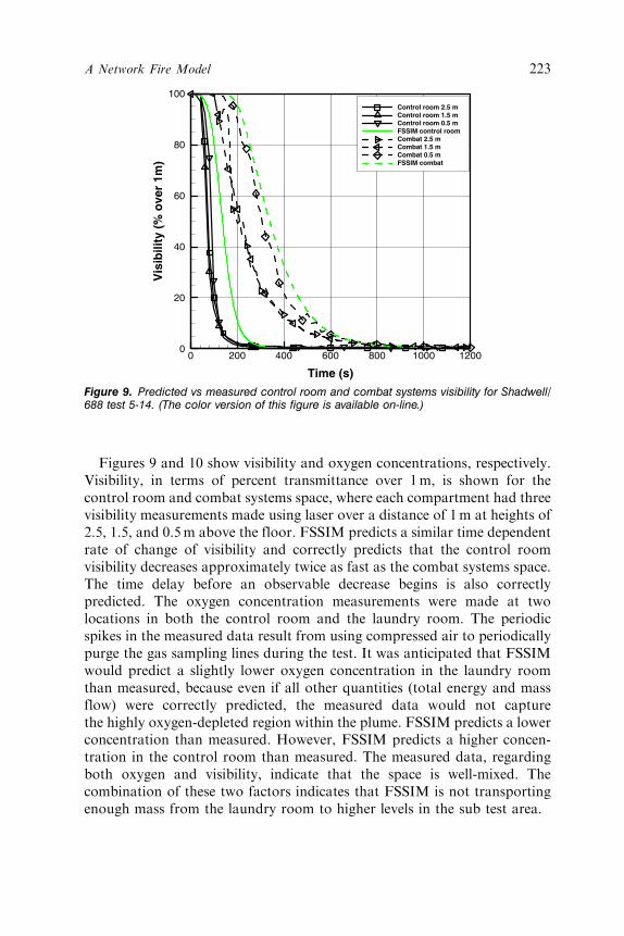
Figures 9 and 10 show visibility and oxygen concentrations, respectively.Visibility, in terms of percent transmittance over 1m, is shown for thecontrol room and combat systems space, where each compartment had threevisibility measurements made using laser over a distance of 1m at heights of2.5, 1.5, and 0.5m above the floor. FSSIM predicts a similar time dependentrate of change of visibility and correctly predicts that the control roomvisibility decreases approximately twice as fast as the combat systems space.The time delay before an observable decrease begins is also correctlypredicted. The oxygen concentration measurements were made at twolocations in both the control room and the laundry room. The periodicspikes in the measured data result from using compressed air to periodicallypurge the gas sampling lines during the test. It was anticipated that FSSIMwould predict a slightly lower oxygen concentration in the laundry roomthan measured, because even if all other quantities (total energy and massflow) were correctly predicted, the measured data would not capturethe highly oxygen-depleted region within the plume. FSSIM predicts a lowerconcentration than measured. However, FSSIM predicts a higher concen-tration in the control room than measured. The measured data, regardingboth oxygen and visibility, indicate that the space is well-mixed. Thecombination of these two factors indicates that FSSIM is not transportingenough mass from the laundry room to higher levels in the sub test area.

Time (s)

Vis

ibili

ty (

% o

ver

1m)

0 200 400 600 800 1000 12000

20

40

60

80

100Control room 2.5 mControl room 1.5 mControl room 0.5 mFSSIM control roomCombat 2.5 mCombat 1.5 mCombat 0.5 mFSSIM combat

Figure 9. Predicted vs measured control room and combat systems visibility for Shadwell/688 test 5-14. (The color version of this figure is available on-line.)


Figures 11 and 12, respectively, show predicted and measured velocitiesin the frame bays and in the primary ducts of the HVAC system. InFigure 11, velocities are shown for four of the eight frame bays; therewere two side-by-side in each of the four locations. FSSIM correctly predictsboth the magnitude and the direction of the flow in the frame bays. InFigure 12, velocities are presented for four locations in the HVAC system.These locations are: in the duct connected to the supply blower used duringnormal recirculation mode, in the duct connected to the exhaust blowerused during normal recirculation mode, in the duct connected to the lowpressure blower used during the emergency ventilation mode, and in thebypass duct used as an external fresh air supply (induction) duringthe emergency ventilation mode. The FSSIM predicted velocities in theseducts are being computed from first principles using manufacturer-suppliedfan curves and the flow losses and lengths associated with all the individualcomponents in the HVAC system. Considering this, the FSSIM predictionsare excellent.

Time (s)

O2

o

nce

ntr

atio

n (

%)

0 200 400 600 800 1000 120017

18

19

20

21

Control room upperControl room lowerLaundry upperLaundry lowerFSSIM CRFSSIM laundry

c

Figure 10. Predicted vs measured control room and laundry room oxygen concentrations forShadwell/688 test 5-14. (The color version of this figure is available on-line.)


Time (s)

Vel

oci

ty (

m/s

)

0 200 400 600 800 1000 1200-12

-10

-8

-6

-4

-2

0

2

4

6

8

10

12

SupplyExhaustEmergencyInductionFSSIM supplyFSSIM exhaustFSSIM emergencyFSSIM induction

Figure 12. Predicted vs measured HVAC system velocities for Shadwell/688 test 5-14. (Thecolor version of this figure is available on-line.)

Time (s)

Vel

oci

ty (

m/s

)

0 200 400 600 800 1000 1200-0.5

0.5

1.5

2.5

3.5

4.5

Crew portCrew stdbWard portWard stdbFSSIM crew portFSSIM crew stdbFSSIM ward portFSSIM ward stdb

Figure 11. Predicted vs measured frame bay velocities for Shadwell/688 test 5-14. (Thecolor version of this figure is available on-line.)


CONCLUSIONS

A new software tool for modeling fire growth and smoke transport hasbeen developed. The goal of the development was to create a stable programcapable of modeling fires in complexly interconnected structures withmultiple HVAC subsystems for the purpose of modeling shipboard fires.The limited validation shown in this paper demonstrates the accuracy andthe capability of this new tool.

In a direct comparison with both CFAST and FDS, FSSIM performedwell in predicting the averaged quantities for a single compartment witha fire and a vent opening. While, as expected, its predictions did not matchthe accuracy of FDS, FSSIM performed as well or better than CFAST inpredicting compartment temperature change, vent mass flow, and neutralplane height.

A second validation was shown using the 688 submarine test areaonboard the ex-USS Shadwell. The complexity of this test area wouldhave been costly to model with FDS. The three separate ventilation systemsand the complexity of their interactions exceeded the CFAST solver’sability to converge. FSSIM was capable of accurate, real-time comput-ing of the spread of smoke and energy through the sub test area.Temperatures, gas concentrations, and mass flows were correctly predictedthroughout the sub test area in both compartments and HVAC systemcomponents.

This first version of FSSIM is a success. It has met the goal of makingaccurate predictions of fire and smoke spread onboard a naval vessel.Further development of FSSIM, not covered in this paper, includesmodeling detection and suppression systems, fire spread, progressiveflooding, and runtime interaction with other software tools, including theautomated extraction of geometric and systems information from digitaldesign documents.

NOMENCLATURE

RomanA¼ area (m2)c¼ specific heat (J/(kgK) )cp¼ constant pressure specific heat (J/(kgK))E¼ energy (J)F¼ function or view factorg¼ gravitational acceleration (9.80665m/s2)h¼ enthalpy (J/kg) or heat transfer coefficient (W/(m2K) )


K¼ form loss factork¼ thermal conductivity (W/(mK))L¼ length (m)M¼mass (kg)mw¼molecular weight (kg/mol)P¼ pressure (Pa)_qq¼ heat transfer rate (W)R¼ real gas constant (8.314472Nm/(molK) )T¼ temperature (K)t¼ time (s)V¼ volume (m3)v¼ velocity (m/s)x¼ position (m)z¼ vertical position (m)

Greek�¼ absorptivity (m�1)�¼miscellaneous multiplier (i.e., relaxation factor)�¼ change in"¼ emissivity or wall roughness (m)�¼ density (kg/m3)� ¼ Stefan–Boltzman constant (5.6704� 10�8W/(m2K4) ) or

direction function (1 or �1)� ¼ transmission factor or time constant (s)

Superscripts00 ¼ per unit area (m�2)d¼ donor (upwind) quantityn¼ next time step

nþ¼ next time step guessn�¼ prior iteration

n� 1¼ prior time stepSubscripts

air¼ airex¼ exchangei¼ compartmentj¼ junctionk¼ compartmentw¼ surface

Overscripts.¼ time derivative (s�1)

�¼ linearized value at next time step or modified net radiationterm

¼ averaged quantity


REFERENCES

1. Floyd, J.E., Hunt, S.P., Williams, F.W. and Tatem, P.A., Fire and Smoke Simulator(FSSIM) Version 1 – Theory Manual, NRL/MR/6180—04-8765, Naval ResearchLaboratory, Washington, DC, 2004.

2. Gaunt, R., Cole, R, Erickson, C., Gido R., Gasser, R., Rodriguez, S. and Young, M.,MELCOR Computer Code Manuals: Reference Manuals Version 1.8.5, NUREG/CR-6119, US Nuclear Regulatory Commission, Vol. 2, Rev. 2, Washington, DC, 2000.

3. Williams, F., Nguyen, X., Buchanan, J., Farley, J., Scheffey, J., Wong, J., Pham, H. andToomey, T., ex-USS Shadwell (LSD-15) – The Navy’s Full-Scale Damage Control andRDT&E Test Facility, NRL/MR/6180—01-8576, Naval Research Laboratory,Washington, DC, 2001.

4. Floyd, J., Scheffey, J., Haupt, T., Habbash, H., Hodge, B., Norton, O., Williams, F. andTatem, P., Requirements and Development Plan for a Shipboard Network Fire Model,NRL Ltr. Rpt. Ser 6180/0469, Naval Research Laboratory, Washington, DC, 2003.

5. Dols, W., Walton, G. and Denton, K., CONTAMW 1.0 User Manual: Multizone Airflowand Contaminant Transport Analysis Software, NISTIR 6476, Building and Fire ResearchLaboratory, National Institute of Standards and Technology, Gaithersburg, MD, 2000.

6. Nichols, B.D. and Gregory, W.S., FIRAC User’s Manual: A Computer Code to SimulateFire Accidents in Nuclear Facilities, NUREG/CR-4561 (LA-10678-M), Los AlamosNational Laboratories for the Nuclear Regulatory Commission, 1986.

7. McGrattan, K., Forney, G., Floyd, J. and Hostikka, S., Fire Dynamics Simulator(Version 3) – User’s Guide, NISTIR-6784, 2002 ed., National Institute of Standards andTechnology, Gaithersburg, MD, 2002.

8. Jones, W., Forney, G., Peacock, R. and Reneke, P., A Technical Reference for CFAST:An Engineering Tool for Estimating Fire Growth and Smoke Transport, NIST TechnicalNote 1431, National Institute of Standards and Technology, Gaithersburg, MD, 2000.

9. Childs, K.W., Heating 7.2 User’s Manual, ORNL/TM-12262, Oak Ridge NationalLaboratory, Oak Ridge, TN, 1993.

10. Cooper, L., Calculation of Flow Through a Horizontal Ceiling/Floor Vent, NISTIR89-4052, National Institute of Standards and Technology, Gaithersburg, MD, 1989.

11. Holman, J., Heat Transfer, 7th ed., Mc-Graw Hill. New York, NY. 1990.

12. Strauss, W., Partial Differential Equations: An Introduction, John Wiley & Sons.New York, NY. 1992.

13. George, T., Wiles, L. Claybrook, S. Wheeler, C. McElroy, J. and Singh, A., GOTHICContainment Analysis Package Technical Manual Version 7.0, EPRI RP4444-1, ElectricPower Research Institute, Inc., Palo Alto, CA, 2000.

14. Forney, G., Computing Radiative Heat Transfer Occurring in a Zone Fire Model, NISTIR4709, National Institute of Standards and Technology, Gaithersburg, MD, 1991.

15. Back, G., Mack, E., Peatross, M., Scheffey, J., White, D., Williams, F., Farley, J.and Satterfield, D., A Methodology for Predicting Fire and Smoke Spread Followinga Weapon Hit, NRL/MR/6180—03-8708, Naval Research Laboratory, Washington,DC, 2003.

16. Wieczorek, C., Vandsburger, U. and Floyd J., ‘‘An Evaluation of the Global EquivalenceRatio Concept for Compartment Fires: Part I – Effect of Experimental Measurements,’’Journal of Fire Protection Engineering, Vol. 14, No. 2, 2004, pp. 9–32.

17. Steckler, K., Quintiere, J. and Rinkinen, W., Flow Induced by Fire in a Compartment,NBSIR 82-2520, National Bureau of Standards (NIST), Gaithersburg, MD, 1982.

18. Steckler, K., Baum, H. and Quintiere, J., Flow Induced Flows Through Room Openings –Flow Coefficients, NBSIR 83-28010, National Bureau of Standards (NIST), Gaithersburg,MD, 1984.


19. Hoover, J., Tatem, P. and Williams, F., Meta-Analysis of Data from the SubmarineVentilation Doctrine Test Program, NRL/MR/6180—98-8168, Naval ResearchLaboratory, Washington, DC, 1998.

20. Parker, A., Scheffey, J., Hill, S., Farley, J., Tatem, P., Williams, F., Satterfield, D.,Toomey, T. and Runnerstrom, E., Full-Scale Submarine Ventilation Doctrine and TacticsTests, NRL/MR6810—98-8172, Naval Research Laboratory, Washington, DC, 1998.


a network fire model for the simulation of fire growth and

Documents